fabien montiel, v. a. squire, and l. g. bennetts ... · under consideration for publication in j....

SUBMITTED VERSION

Fabien Montiel, V. A. Squire, and L. G. Bennetts Attenuation and directional spreading of ocean wave spectra in the marginal ice zone Journal of Fluid Mechanics, 2016; 790:492-522 © Cambridge University Press 2016

Originally Published at: http://dx.doi.org/10.1017/jfm.2016.21

http://hdl.handle.net/2440/97888

PERMISSIONS

http://journals.cambridge.org/action/displaySpecialPage?pageId=4608

Content is made freely available by the author

This is achieved by depositing the article on the author’s web page or in a suitable public repository,

often after a specified embargo period. The version deposited should be the Accepted Manuscript.

Publishers typically impose different conditions, but it should be noted that many OA mandates (such

as the NIH public access policy) specify the Accepted Manuscript in their requirements unless the

publisher allows the Version of Record. Refer to the table below for details.

Summary of where an author published in a Cambridge Journal may deposit versions of their

article

7 March 2016

http://dx.doi.org/10.1017/jfm.2016.21

http://hdl.handle.net/2440/97888

http://journals.cambridge.org/action/displaySpecialPage?pageId=4608

Under consideration for publication in J. Fluid Mech. 1

Attenuation and directional spreading ofocean wave spectra in the marginal ice zone

Fabien Montiel1†, V. A. Squire1 and L. G. Bennetts2

1Department of Mathematics and Statistics, University of Otago, PO Box 56, Dunedin 9054,New Zealand

2School of Mathematics Sciences, University of Adelaide, Adelaide 5005, Australia

(Received ?; revised ?; accepted ?. - To be entered by editorial office)

A theoretical model is used to study wave energy attenuation and directional spreadingof ocean wave spectra in the marginal ice zone (MIZ). The MIZ is constructed as an arrayof tens of thousands of compliant circular ice floes, with randomly selected positions andradii determined by an empirical floe size distribution. Linear potential flow and thinelastic plate theories model the coupled water-ice system. A new method is proposed tosolve the time-harmonic multiple scattering problem under a multi-directional incidentwave forcing with random phases. It provides a natural framework for tracking the evo-lution of the directional properties of a wave field through the MIZ. The attenuationand directional spreading are extracted from ensembles of the wave field with respect torealizations of the MIZ and incident forcing randomly generated from prescribed distribu-tions. The averaging procedure is shown to converge rapidly so that only a small numberof simulations need to be performed. Far field approximations are investigated, allowingefficiency improvements with negligible loss of accuracy. A case study is conducted for aparticular MIZ configuration. Observed exponential attenuation of wave energy throughthe MIZ is reproduced by the model, while the directional spread is found to grow linearlywith distance. Directional spreading is shown to weaken when the wavelength becomeslarger than the maximum floe size.

Key words:

1. Introduction

There is now growing evidence that ocean surface waves have a significant impacton the seasonal advance and retreat of sea ice in Arctic and Southern Oceans. Satelliteobservations have shown that the energy content of wave spectra in the polar oceanshas been trending upwards in the last three decades, more significantly than at lowerlattitudes (Young et al. 2011). Recent in situ observations and hindcasts of energeticwave fields at high lattitudes (Thomson & Rogers 2014; Kohout et al. 2014; Collins et al.2015) support these long-term trends and suggest an increasing impact of waves on themorphology of ice-covered oceans. In particular, waves contribute to the rapid decline ofsea ice extent and thickness observed in the Arctic region (Laxon et al. 2013; Meier et al.2013) by fracturing the elastic ice cover under sufficient flexural load (see Squire et al.1995; Squire 2007, for reviews), and therefore accelerating the melting of sea ice. Thiscontribution is most pronounced within, say, 100 km of the ice edge, a region referred to

† Email address for correspondence: [email protected]

2 F. Montiel, V. A. Squire and L. G. Bennetts

as the marginal ice zone (MIZ), which typically consists of a disordered array of floatingice floes with various shapes and characteristic horizontal dimensions O (10–100m).The presence of a broken-up ice cover with a certain ice concentration (the fraction of

sea surface covered by ice), thickness and floe size distribution (FSD) governs the evo-lution of wave spectral properties (energy content, frequency and direction) within theMIZ. When ocean waves enter an MIZ they are attenuated and, for modest seas, muchevidence now supports the assertion that ocean wave energy decays at an exponentialrate with distance from the ice edge (see Squire & Moore 1980; Wadhams et al. 1988;Meylan et al. 2014, for field measurements in both the Arctic and Southern Oceans).Moreover, the rate of attenuation tends to increase with decreasing wave period. Con-comitantly, the range of directions over which waves travel in the MIZ appears to increasewith distance from the ice edge, so that the the wave spectrum tends to become fullyisotropic. Directional spreading in the MIZ has been observed during the field work ofWadhams et al. (1986) and can also been inferred from SAR imagery (see, e.g., Liu et al.1991b). Both wave energy attenuation and directional spreading are governed by a com-bination of scattering effects and dissipative processes. Wave energy dissipation occursin many different forms, e.g. collisions (Shen & Squire 1998; Bennetts & Williams 2015),turbulence (Liu & Mollo-Christensen 1988), wave overwash (Bennetts et al. 2015; Skeneet al. 2015), floe breakup (Williams et al. 2013a) and inelastic bending (Squire & Fox1992). Estimating their effects on wave energy attenuation is a difficult task, as most arenon-linear processes. Although simplified empirical parameterizations have been devel-oped to model the MIZ as a homogeneous linearly viscoelastic layer (Wang & Shen 2010),their validity is unresolved and calibration presents a major challenge that requires moredata than are currently available (Mosig et al. 2015). In contrast, wave scattering is con-servative and redistributes the wave energy over the directional domain. The exponentialattenuation of wave energy and directional spreading is a direct consequence of linearmultiple scattering theory for waves propagating in random media. This effect has beenobserved and modelled in many areas concerned with such processes (see, e.g., Ishimaru1978).Herein a three-dimensional model of wave energy attenuation and directional spread-

ing in the MIZ is proposed. Our goal is to reproduce observed wave attenuation anddirectional spreading of ocean wave spectra as they propagate through the MIZ, by mod-elling the random nature of open ocean sea states and the disorder of the distributionof ice floes in the MIZ. The primary outcome will be an improved parameterization ofwave/sea ice interactions in ice/ocean models (IOMs), e.g. TOPAZ, and spectral wavemodels (SWMs) such as Wavewatch III R⃝ or WAM. We plan to use our model simulationsto generate attenuation and directional spreading parameters in the form of look-up ta-bles. We note that at present only two-dimensional approaches (i.e. those with one wavedirection) are employed to model wave energy attenuation in such large scale models,with no exchange of energy between different wave directions (see Rogers & Orzech 2013;Doble & Bidlot 2013; Williams et al. 2013a,b, for implementation in SWMs and IOMs).Unidirectional wave energy attenuation in the MIZ, i.e. neglecting directional spread-

ing, due to multiple scattering by arrays of ice floes has been described theoretically anumber of times within the framework of linear potential flow theory (see Squire et al.1995; Squire 2011, for reviews). The most common representation of each floe is a thinelastic plate. For example, Kohout & Meylan (2008) considered transmission of wavesthrough multiple elastic plates floating with no submergence, using a two-dimensionalmodel with one vertical dimension and one horizontal dimension. They used ensembleaveraging to show that selecting floe lengths and floe spacings randomly from Rayleighdistributions leads to exponential attenuation of the proportion of mean wave energy

Directional waves in the marginal ice zone 3

transmitted with respect to the number of floes, and that the effective rate of atten-uation increases with decreasing wave period. These behaviours mirror those of oceanwaves in the MIZ. Kohout & Meylan further showed that their scattering model predictsattenuation rates comparable to those measured in the MIZ for mid-range wave peri-ods (approximately 6 to 15 s) but that it underpredicts the attenuation rates of longerperiod waves by at least an order of magnitude. Bennetts & Squire (2012b) derived asemi-analytic expression for the rate of exponential attenuation predicted by the two-dimensional model based upon the reflection produced by a solitary floe, assuming thewave phase between floes is random, as opposed to varying the floe lengths and spacings.They also included a parameterization of wave energy dissipation due to interaction withthe floes via the viscoelastic plate model of Robinson & Palmer (1990) to correct forattenuation of long-period waves. Bennetts & Squire (2012a) subsequently went on toconsider how sensitive the rate of exponential decay was to physical parameters in theirmodel, with the direct purpose of intelligently assimilating wave-ice interactions in a con-temporary IOM for the first time. Williams et al. (2013a,b) used the model of Bennetts& Squire (2012b) to move towards this goal. Although these authors considered wavevectors from different directions, the scattering was inherently one-dimensional with nochanges to the directional structure of the wave spectrum being possible.Several papers have outlined three-dimensional scattering models (two-dimensional

waves) to predict attenuation through the MIZ. However, for the thousands of floesneeded to simulate the MIZ, the computational expense of the additional dimension hasled to the use of approximations and/or simplifications of the geometry. For example,Meylan et al. (1997) approximated the wave interactions between floes using the transporttheory of radiative transfer in random media (based on the Boltzman equation; seeIshimaru 1978), which does not resolve wave phases. They used the solitary circularelastic floe model of (Meylan & Squire 1996) to calculate the scattering kernel. Theyshowed that, without an energy dissipation term, i.e. for scattering alone, wave energyattenuates for a finite distance only, after which it remains constant. Meylan & Masson(2006) showed that the model of Meylan et al. (1997) is almost identical to that ofMasson & Leblond (1989), who restricted their ice floe model to be a floating rigidcylinder. Bennetts et al. (2010) proposed a model based on full potential flow theory,using the methods devised by Bennetts & Squire (2009) and Peter & Meylan (2009).They considered square elastic floes in addition to circular floes, but found the shapehad minimal effect on predicted attenuation rates. They showed the model gave excellentagreement with the measurements of Squire & Moore (1980) for mid-range periods but,again, significantly underestimated the attenuation on long period waves. Further, theystudied evolution of the directional spectrum of plane incident waves through the MIZ.However, for computational expediency, they imposed artificial periodic repetitions of afloe or groups of floes. This meant the wave field was composed of plane waves travellingin a handful of different directions, where the exact number changed at certain waveperiods. This led to artificial jumps in the attenuation rate with respect to wave periodand no spreading of energy over the directional range was observed.The three-dimensional model of wave attenuation and directional spreading in the MIZ

proposed here is a solution of the full linear equations of potential flow theory and doesnot invoke artificial periodicity on the geometry. It extends the solution method proposedby Montiel et al. (2015a) for a two-dimensional problem of acoustic wave propagationthrough a large, finite array of identical circular obstructions. We include a realisticpower-law FSD, which is based on the observational studies of Rothrock & Thorndike(1984) and Toyota et al. (2006, 2011). Moreover, we model the incident wave forcing as arandom sea state with a prescribed directional energy distribution. Ensemble averaging


is then used to compute the wave energy attenuation and directional spreading throughthe MIZ.

2. Preliminaries

2.1. Governing equations

Consider a three-dimensional seawater domain with infinite horizontal extent and con-stant finite depth, h say. Points in the water are located by Cartesian coordinates (x, y)in the horizontal plane and z in the vertical direction positively oriented upwards. Weassume that the free surface at rest coincides with the plane z = 0 so the seabed isdefined by z = −h. Irregularities in the seabed are not considered here, as h is assumedto be large compared to the wavelength throughout this study.We seek to model the propagation of a directional ocean wave spectrum through a MIZ

composed of thousands to tens of thousands of randomly positioned floating, compliantice floes with circular shape and uniform thickness. We only consider circular ice floesfor simplicity, conjecturing that the shape of the floes has a small effect on the meanproperties of wave propagation through large random arrays.The solution method described in § 3 requires clustering the array of floes into multiple

slabs. Without loss of generality, we align the slabs with the y-axis. Let S denote thenumber of slabs, and let slab q be bounded by ξq−1 ⩽ x ⩽ ξq, 1 ⩽ q ⩽ S, have widthLq = ξq − ξq−1 and contain Nq floes. A sketch of the geometry is given in figure 1. Notethat a floe belongs to a slab if its centre is in the slab bounds.Ice floe radii aqp, 1 ⩽ q ⩽ S, 1 ⩽ p ⩽ Nq, are drawn from a prescribed power-law

FSD as observed in the field (Toyota et al. 2006). A parameterization of the FSD willbe described in § 5.2. Further, we assume that all floes have constant thickness D anduniform density ρ ≈ 922.5 kgm−3. We do not include floes with different thickness anddensities in the model in order to limit the number of parameters, although the methodwe propose can accommodate these extensions.We consider a multi-directional wave field with small amplitude compared to the wave-

length and prescribed angular frequency ω. The water is approximated as an inviscidand incompressible fluid with constant density ρ0 ≈ 1025 kgm−3 and irrotational flow.The linear theory of water waves can then be used to describe the water motion. As-suming time-harmonic conditions, we express the velocity field in the water domain as(∇, ∂z)Re

{(g/ iω)ϕ(x, y, z) e− iωt

}, where ∇ ≡ (∂x, ∂y) and g ≈ 9.81m s−2 is accelera-

tion due to gravity. The complex-valued (reduced) potential, ϕ, is governed by Laplace’sequation

∇2ϕ+ ∂2zϕ = 0 (−∞ < x, y < ∞,−h < z < −d) , (2.1)

where z = −d describes the upper boundary of the fluid domain, such that d = 0 when afree surface is present and d = (ρ/ρ0)D (i.e. the Archimedean draught) when the surfaceis covered by a floe. On the impermeable seabed, we prescribe a no-normal-flow condition

∂zϕ = 0 (z = −h) . (2.2)

In fluid regions bounded above by a free surface (i.e. d = 0), the potential satisfies theboundary condition

∂zϕ = αϕ (z = 0), (2.3)

where α = ω2/g is a frequency parameter.We prescribe an ambient incident wave field ϕIn travelling in the positive x-direction

and defined by a superposition of plane waves with amplitudes that depend continuously


Figure 1. Schematic of the geometry in the horizontal plane z = 0.

on the angle of incidence τ (with respect to the x-axis). We express it as

ϕIn(x, y, z) = ζ0(z)

∫ π/2

−π/2

AIn(τ) e ik0((x−ξ0) cos τ+y sin τ) dτ, (2.4)

where the incident wave directional spectrum AIn(τ) characterizes the angular distribu-tion of ambient wave amplitude at x = ξ0. The function ζ0(z) = cosh k0(z+ h)/ cosh k0hdescribes the vertical motion of the incident wave field. The quantity k0 denotes the prop-agating wavenumber for a wave travelling in the free-surface region and will be definedshortly. Scattering of the ambient wave field by the array of floes gives rise to reflectedand transmitted wave components that are expressed as

ϕ(x, y, z) ≈ ϕIn(x, y, z) + ζ0(z)

∫ π/2

−π/2

AR(τ) e ik0(−(x−ξ0) cos τ+y sin τ) dτ (2.5a)

as x → −∞ and

ϕ(x, y, z) ≈ ζ0(z)

∫ π/2

−π/2

AT(τ) e ik0((x−ξS) cos τ+y sin τ) dτ (2.5b)

as x → ∞. The reflected and transmitted wave directional spectra, AR(τ) and AT(τ),are unknowns of the problem. They characterize the angular distribution of the reflectedand transmitted amplitudes at x = ξ0 and x = ξS , respectively.We model the motion experienced by the ice floes using the Kirchhoff-Love theory of

thin elastic plates, which assumes that thickness is small compared to diameter and ver-tical deformations are small relative to thickness. At the water-floe interface the potential


then satisfies

(β∇4 + 1− αd)∂zϕ = αϕ (z = −d), (2.6)

for a floe with thickness D and draught d = (ρ/ρ0)D. The stiffness parameter β = F/ρ0gis defined in terms of the flexural rigidity of the plate F = ED3/12(1 − ν2), whereE ≈ 6GPa is a typical value for the effective Young’s modulus of sea ice (Mellor 1986)and ν ≈ 0.3 denotes Poisson’s ratio.We complete the description of the ice floe model by imposing free edge conditions.

These are most conveniently expressed using the polar coordinates (r, θ) with origin atthe centre of the floe. For a floe of radius a, we have[

r2∇2r,θ − (1− ν)

(r∂r + ∂2

θ

)]∂zϕ = 0 (r = a) (2.7a)

and [r3∂r∇2

r,θ + (1− ν) (r∂r − 1) ∂2θ

]∂zϕ = 0 (r = a), (2.7b)

where ∇r,θ ≡ (∂r + 1/r, (1/r)∂θ). In addition, we assume that the floes do not respondin surge and sway, so that

∂rϕ = 0 (r = a, −d < z < 0). (2.7c)

2.2. Scattering by a single floe

Each floe scatters the local wave field incident on it, which is the combination of theambient incident wave field and the wave fields scattered by all other floes. For a givenfloe, which, as above, is assigned the polar coordinate system (r, θ), these local incidentand scattered wave potentials are expressed as the truncated eigenfunction expansions

ϕI(r, θ, z) ≈M1∑m=0

ζm(z)

N∑n=−N

am,nJn(kmr) e inθ (r > a) (2.8a)

and

ϕS(r, θ, z) ≈M1∑m=0

ζm(z)

N∑n=−N

bm,nHn(kmr) e inθ, (r > a) (2.8b)

respectively, which are solutions to (2.1)–(2.3) in cylindrical coordinates (see, e.g., Peteret al. 2003, for a detailed derivation). We have introduced Jn and Hn to denote the Besseland Hankel functions of the first kind of order n, respectively. The amplitudes am,n andbm,n, 0 ⩽ m ⩽ M1, −N ⩽ n ⩽ N , are unknowns of the scattering problem. We definethe vertical modes as ζm(z) = cosh km(z + h)/ cosh kmh. The wavenumbers km, m ⩾ 0,are the solutions k of the dispersion relation for an open water region, that is

k tanh kh = α. (2.9)

We denote the positive real root of (2.9) by k0. It is associated with a wave modetravelling in the horizontal plane. As water depth h was assumed to be large comparedto the wavelength, we have k0 ≈ α, so that the wavelength is approximately independentof h. All other km, m ⩾ 1, are purely imaginary with positive imaginary part and areordered such that − ikm < − ikm+1. They are associated with evanescent vertical wavemodes which decay exponentially in the horizontal directions, such that the rate of decayincreases for increasing m. In contrast to k0, the values of km, m ⩾ 1, depend on h. Notethat the sums in (2.8) are truncated versions of the corresponding series expansions, withM1 and N chosen in order to obtain a sufficient degree of accuracy (see below).Montiel et al. (2013) proposed a solution method for the single floe scattering problem.

Using equations (2.1), (2.2), (2.6), (2.7a) and (2.7b) they expressed the potential below


the floe (i.e. r < a) as a truncated series of eigenfunctions similar to (2.8a), but withdifferent wavenumbers characterizing wave modes in the ice-covered water domain. Theythen used a version of the eigenfunction matching method (EMM) which accommodatesthe draught of the floe, through (2.7c), in order to extend the zero-draught EMM of Peteret al. (2003). The EMM produces a mapping between the amplitudes am,n and bm,n foreach angular mode n; the axisymmetry of the problem decouples the angular modes. Inmatrix form, the mapping is expressed as

bn = Snan, (2.10)

for −N ⩽ n ⩽ N , where an and bn are column vectors of size M1 + 1 containing theamplitudes am,n and bm,n, respectively, for a given n. Matrices Sn are square of sizeM + 1 and form the diffraction transfer matrix (DTM) of the floe when concatenatedin a block diagonal matrix. Extensions of our model to arbitrarily-shaped floes couldbe accommodated following Peter & Meylan (2004) who devised a numerical method tocompute the DTM of such floes. Note that in this case the DTM loses its block-diagonalproperty.We choose the truncation limits N and M1 to achieve three digit accuracy for the

scattered energy. In the regime of interest here, k0a =O(1), this typically requires M1 =O(100) vertical modes, and N =O(1) angular modes, as demonstrated by Montiel (2012).

2.3. Multiple scattering and limitations of the direct approach

Our goal is to solve the wave scattering problem deterministically for a large number offloes. Apart from truncations, no approximation will be made with regards to multiplescattering by the array, so that the scattered field due to each floe acts as an incidentfield on all the other floes.The so-called self-consistent approach (or direct matrix method) provides an exact

representation of multiple scattering processes and was introduced in the context ofocean wave interactions with floating structures by Kagemoto & Yue (1986), noting thatthis approach is standard in many areas concerned with wave scattering by arrays ofscatterers (see, e.g., Martin 2006). The method is briefly summarized below and thereader is referred to the investigations cited here for additional details (see also Peter &Meylan 2004, in the context of wave interactions with elastic ice floes).

The method describes the wave forcing ϕ(p)I incident upon a floe p, which has its centre

located at (x, y) = (xp, yp), as the coherent sum of the ambient incident wave ϕIn andthe scattered wave fields originating from all the other floes, i.e.

ϕ(p)I = ϕIn +

∑j, j =p

ϕ(j)S , (2.11)

where ϕ(j)S is the scattered wave potential due to a floe j, with centre located at (x, y) =

(xj , yj), and the sum over j runs for all floes in the array except p. The incident andscattered wave components are expressed in terms of the eigenfunction expansions (2.8),using the relevant local polar coordinates (rp, θp), defined by (x, y) = (xp+rp cos θp, yp+

rp sin θp). Subsequently, the expressions for the scattered waves ϕ(j)S in (2.11) are mapped

into the local coordinates (rp, θp) of floe p. Application of the (reduced) boundary con-dition (2.10) around floe p then yields the following matrix equation

b(p)n −

∑j, j =p

N∑s=−N

S(p)n T(j,p)

n,s b(j)s = S(p)

n f (p)n , (2.12)

which can be obtained for all floes p. Numerical experiments (see § 4) have shown that


O(1) vertical modes only are necessary in (2.8) to resolve wave interactions in an array offloes accurately, assuming the single floe solutions are obtained with sufficient accuracy(which requires M1 =O(100) vertical modes). The vectors of scattered wave amplitudes

b(p)n and matrices S

(p)n in (2.12) are then chosen to have size M2 + 1, where M2 =O(1).

They are obtained by truncating the corresponding quantities of size M1 + 1 defined forthe single floe solution.

The resulting system of equations is solved for the scattered wave amplitudes b(p)n

for all floes p and angular modes n. Here the forcing vectors f(p)n , −N ⩽ n ⩽ N ,

contain the amplitudes of the ambient incident potential (2.4) expressed in the lo-

cal cylindrical coordinates of floe p. Square matrices S(p)n are analogous to the matri-

ces defined in (2.10) for each floe p. We have also introduced the diagonal matrices

T(j,p)n,s = diag

{Hs−n(kmRj,p) e

i(s−n)ϖj,p , 0 ⩽ m ⩽ M2

}of size M2+1, where (Rj,p, ϖj,p)

are the polar coordinates of the centre of floe p in the local system associated with floej. These matrices describe the change of local polar coordinates from floe j to floe p andtheir entries are calculated using Graf’s addition theorem (Abramowitz & Stegun 1970),which couples the angular modes.The size of system (2.12) grows linearly with the number floes in the array and di-

rect inversion will lead to a computational cost increasing with the cubic power of thenumber of floes. The order-of-scattering method, based on the original paper by Twer-sky (1952), has been used to approximate the solution of (2.12) by successive orders ofmultiple scattering events (see, e.g., Ohkusu 1974; Mavrakos & Koumoutsakos 1987).Mathematically, this is equivalent to solving (2.12) using an iterative scheme, e.g. the Ja-cobi or Gauss-Seidel method. This method usually leads to performance improvements,although computational cost is strongly affected by the concentration of floating bodiesin the array (Kagemoto & Yue 1986). Numerical experiments conducted by the authorshave shown that direct inversion or iterative approaches are limited to arrays of O(100)floes.

3. Slab-clustering method

We remedy the practical shortcoming of the self-consistent approach by implementingthe slab-clustering method, described by Montiel et al. (2015a) for a cognate canonicalacoustic problem. While much of the method presented by Montiel et al. may be appliedstraightforwardly to the present problem, the existence of evanescent vertical modes addsa complication that needs to be dealt with carefully.The method consists of dividing the array of floes into slabs as described in §2.1 We

seek a solution for the wave field between two adjacent slabs as the coherent superpositionof the left-travelling and right-travelling directional wave fields. In its most general form,the field at x = ξq can be expressed as

ϕq(x) = ϕ(+)q (x) + ϕ(−)

q (x), (3.1)

where

ϕ(±)q (x) ≈

M2∑m=0

ζm(z)

∫Γm

(A±

m;q(χ) eikm(±(x−ξq) cosχ+y sinχ)

)dχ, (3.2)

for 0 ⩽ q ⩽ S. The A±m;q(χ) represent rightward (+) and leftward (−) amplitude functions

corresponding to wave modes travelling (m = 0) and decaying (m ⩾ 1). The amplitudesA+

m;q−1 and A−m;q are incident on slab q from its left and right, respectively, and A−

m;q−1

and A+m;q are scattered by it to the left and right, respectively.


Figure 2. The left-hand panel shows the integration contours Γ0 (blue solid) and Γe (greendashed) in the complex χ-plane, which describe the domains of the amplitude functions A±

m;q(χ)for travelling (m = 0) and evanescent (m ⩾ 1) vertical modes, respectively. The arrows indicatethe directions of the contours. The right-hand panel shows the corresponding truncated contours

Γ0 (blue solid) and Γe (green dashed) used in the numerical approximation discussed in § 3.2.

The integration contour Γm differs for the travelling (m = 0) and evanescent (m ⩾ 1)modes. For a travelling mode, it runs from −π/2 + i∞ to π/2− i∞ through the originand is parameterized by

χ(ς) =

−π/2− i(1 + ς) (−∞ ⩽ ς ⩽ −1),π/2ς (−1 ⩽ ς ⩽ 1),

π/2 + i(1− ς) (1 ⩽ ς ⩽ ∞).(3.3)

The contour Γ0 is depicted in figure 2 as a blue solid line (see the left-hand panel). Theintegration contours Γm (m ⩾ 1) for the evanescent vertical modes are all identicallyequal to Γe, which spans the imaginary axis from i∞ to − i∞, as shown in figure 2(see green dashed line in the left panel). The integration contours Γ0 and Γe arise fromdecomposing a surface wave source into a superposition of plane waves continuouslydepending on the complex angular parameter χ, as will be shown in § 3.1.The complex branches of Γ0 correspond to wave components that decay exponentially

in the x-direction. The rate of decay increases as the imaginary components of χ getlarger. In this regard, these components are similar to the evanescent modes.We introduce an approximation for computational purposes, by truncating Γe and

the complex branches of Γ0 to ±γ i and ±(π/2 − γ i), respectively, where γ ⩾ 0. The

truncated contours are denoted by Γ0 and Γe and are shown in the right-hand panel offigure 2. Note that the special case γ = 0 represents a far-field approximation, for whichall x-decaying wave components are neglected in interactions between slabs. Its validitydepends on the spacing between slabs and will be discussed further in § 4.

3.1. Reflection and transmission by a single slab

Montiel et al. (2015b) derived a set of relationships (for the special case γ = 0) betweenthe incident and scattered amplitude functions A±

0;q(χ) on either side of a given slab q


as a result of reflection and transmission. Here we extend these relationships to includeevanescent vertical modes (i.e. m ⩾ 1) and x-decaying wave components (i.e. γ > 0).We consider the scattering by slab q due to the incident forcing from its left-hand

side, ϕ(+)q−1, only. The response to incident forcing from its right-hand side, ϕ

(−)q , follows

similarly, and the total response to forcing from both sides is calculated via superposition.The forcing field may be expressed in the local polar coordinates of floe p analogously

to (2.8b). For each angular mode n and vertical mode m, the forcing amplitudes are thengiven by [

f (p)n

]m

= in∫Γm

A+m;q−1(χ) e

− inχ e ikm((xp−ξq−1) cosχ+yp sinχ) dχ. (3.4)

The self-consistent method outlined in §2.3 is used to solve the multiple scatteringproblem within the slab. It results in a system of equations analogous to (2.12) whichyields the mapping

b[q] = D[q]f [q], (3.5)

where b[q] (f [q]) is a vector of length (M2 +1)(2N +1)Nq that contains all the scattered

(incident) wave amplitudes contained in b(p)n (f

(p)n ), for −N ⩽ n ⩽ N and 1 ⩽ p ⩽ Nq.

The square matrix D[q] has size (M2 + 1)(2N + 1)Nq and is the DTM of slab q.We seek the reflected and transmitted amplitude functions in the form

A−m,q−1(χ) =

M2∑l=0

∫Γl

R+m,l;q(χ : τ)A+

l;q−1(τ) dτ (3.6a)

and

A+m,q(χ) =

M2∑l=0

∫Γl

T +m,l;q(χ : τ)A+

l;q−1(τ) dτ, (3.6b)

respectively. The functions R+m,l;q(χ : τ) and T +

m,l;q(χ : τ) are respectively reflection andtransmission kernels for each pair of vertical modes m and l.In order to evaluate the reflection and transmission kernels, we re-express the scattered

wave field (2.8a) due to each floe in the slab as a superposition of plane waves. Thisis achieved using the following plane wave representation of the outgoing cylindricalharmonics

Hn(kmr) e inθ =

(− i)n

π

∫Γm

e inχ e ikm(x cosχ+y sinχ) dχ, (x ⩾ 0)

in

π

∫Γm

e− inχ e ikm(−x cosχ+y sinχ) dχ, (x ⩽ 0),(3.7)

where (x, y) = (r cos θ, r sin θ). This identity is derived from Sommerfeld’s integral rep-resentation of the Hankel function (Sommerfeld 1949) for m = 0, while an integralrepresentation of the modified Bessel functions of the second kind Kn has been used form ⩾ 1 (see Linton & Evans 1992, equation 2.12). To the authors’ knowledge, the twocases have not been unified in this manner before. Substituting (3.7) into (2.8a) for allfloes and modes simultaneously, and using (3.5) and (3.4) in turn, we obtain the follow-ing semi-analytical expressions for the reflection and transmission kernels after algebraicmanipulations

R+m,l;q(χ : τ) =

(vS−m;q(χ)

)trPD[q]P−1vIn+

l;q (τ) (3.8a)

and

T +m,l;q(χ : τ) =

(vS+m;q(χ)

)trPD[q]P−1vIn+

l;q (τ) + e ikmLq cosχδ(χ− τ), (3.8b)


where a superscript tr indicates transpose and δ( . ) denotes the Dirac delta.In these expressions we have defined the vector vIn+

l;q−1(τ) of length Nq(2N+1)(M2+1),which provides a change from Cartesian to polar coordinates of the forcing field in thelocal system of each floe in the slab. Its entries are[

vIn+m;q(τ)

]ind(l,p,n)

= in e− inτ e ikl((xp−ξq−1) cos τ+yp sin τ)δml, (3.9a)

where ind(l, p, n) = lNq(2N+1)+(p−1)(2N+1)+N+n+1 defines the modal hierarchy(vertical mode, floe number, angular mode) in ordering entries, and δml is the Kroneckerdelta. In contrast, the vectors vS−

m;q−1(χ) and vS+m;q(χ) provide a change from polar to

Cartesian coordinates of the scattered field due to each floe, travelling in the leftwardand rightward direction, respectively. Their entries are[

vS−m;q(χ)

]ind(l,p,n)

=in

πe− inχ e ikl((xp−ξq−1) cosχ−yp sinχ)δml (3.9b)

and [vS+m;q(χ)

]ind(l,p,n)

=(− i)n

πe inχ e− ikl((xp−ξq) cosχ+yp sinχ)δml. (3.9c)

The matrix P is a permutation matrix of size Nq(2N + 1)(M2 + 1) used to change themodal hierarchy from that used in the slab DTM D[q] (i.e. floe number, angular mode,vertical mode) to that used in (3.9). Also note that the second term in (3.8b) representsthe contribution from the forcing field to the transmitted field.

3.2. Multiple slabs

At the boundary x = ξq, the left- and right-travelling amplitude functions take the form

A−m,q(χ) =

M2∑l=0

∫Γl

(R+

m,l;q+1(χ : τ)A+l;q(τ) + T −

m,l;q+1(χ : τ)A−l;q+1(τ)

)dτ (3.10a)

and

A+m,q(χ) =

M2∑l=0

∫Γl

(T +m,l;q(χ : τ)A+

l;q−1(τ) +R−m,l;q(χ : τ)A−

l;q(τ))dτ, (3.10b)

where the kernel functionsR±m,l;q and T ±

m,l;q are found using the method described in §3.1.Given that the forcing is provided by (2.4) only, we have A+

0;0(χ) = AIn(χ), A+0;m(χ) = 0

for 1 ⩽ m ⩽ M and A−S;m(χ) = 0 for 0 ⩽ m ⩽ M2.

A numerical scheme is implemented by discretizing the amplitude and kernel functionsusing a uniform sampling of the angular parameters χ and τ . Amplitudes and kernelsassociated with a travelling vertical mode (m = 0) are defined on the truncated contour

Γ0 introduced at the beginning of § 3 (see the right-hand panel of figure 2). Contour Γ0 isthen discretized by selecting 2Ntr + 1 samples χi, −Ntr ⩽ i ⩽ Ntr. Different resolutionsare taken for the sub-interval [−π/2, π/2] of Γ0 and its complex branches. Typically theresolution chosen for the complex branches is 5 times as coarse as that of [−π/2, π/2].

Likewise, contour Γe is discretized using 2Nev + 1 samples.Combining all the vertical modes, we can define vector versions of the amplitude func-

tions A±q containing the value of the corresponding continuous functions A±

m,q(χi) atall angular samples χi. Likewise, we obtain matrix versions of the kernel functions afterdiscretization. At this point, a numerical quadrature must be chosen to approximate theintegrals involved in (3.10). Although high order schemes, e.g. Simpson’s rule or Gaussianquadrature, are very accurate for relatively smooth functions, we expect our spectra to


be noisy for large random arrays of floes (confirmed by numerical experiments), in whichcase lower order quadratures provide more accurate and more efficient estimates. Wefound that a composite trapezoidal rule gave the best results in terms of convergence.The weighting factors of the trapezoidal rule can be assembled in a diagonal matrix ofsize Nang = 2Ntr + 1 +M(2Nev + 1), which multiplies the matrix versions of the kernelfunctions to give the reflection and transmission matrices R±

q and T±q . Consequently,

(3.10) is written in the discretized form

A−q = R+

q+1A+q + T−

q+1A−q+1 and A+

q = T+q A

+q−1 +R−

q A−q . (3.11)

The solution to the slab interaction problem is obtained using an efficient iterativetechnique, which is an extension to the one described by Montiel et al. (2015a) for trav-elling modes only. Following this approach, at each slab boundary x = ξq, the unknownamplitude vectors are given by

A+q =

(I−R−

1,qR+q+1,M

)−1

T+1,qA

+0 (3.12a)

and

A−q =

(I−R+

q+1,MR−1,q

)−1

R+q+1,MT+

1,qA+0 , (3.12b)

where I denotes the identity matrix of order Nang, and R±p,q and T±

p,q are the reflectionand transmission matrices, respectively, for the stack of slabs p to q. These reflectionand transmission matrices are computed iteratively, starting from slab 1 alone, whichinitializes the procedure, to the stack of slabs 1 to S, adding one slab to the stack at eachiteration.We establish a convergence criterion for the numerical integration scheme considered

here, based on the energy conservation relation∫ π/2

−π/2

∣∣AR(χ)∣∣2 dχ+

∫ π/2

−π/2

∣∣AT(χ)∣∣2 dχ =

∫ π/2

−π/2

∣∣AIn(χ)∣∣2 dχ (3.13)

being satisfied within a tolerance of 10−4, where the reflected and transmitted amplitudefunctions are given by AR(χ) = A−

0;0(χ) and AT(χ) = A+0;S(χ), respectively, for −π/2 ⩽

χ ⩽ π/2. Note that we have restricted the integration domain to include travellingwave components only, as they are the only ones to affect the energy balance of thesystem. We refer to the restriction of the amplitude functions A±

0;q(χ), q = 0, . . . , S, to

−π/2 ⩽ χ ⩽ π/2 as directional spectra. In particular, AR(χ) and AT(χ) are the reflectedand transmitted directional spectra, respectively.We further note that although the energy conservation relation (3.13) is necessary for

convergence of our numerical method, it is not sufficient to obtain convergence to thedesired solution. In particular, we can always obtain energy conservation for sufficientlyhigh Nang, regardless of the value taken for the truncation parameter γ and the resolutionof the complex branches in our numerical approximation of the integration contoursΓe and Γ0. Convergence of the solution within the desired tolerance is obtained for asufficiently large γ, as will be shown in § 4.

4. Far-field approximations

The far-field approximations neglect evanescent/decaying wave components in waveinteractions between floes. The first far-field approximation (FFA1) we consider consistsof neglecting the vertical evanescent modes (i.e. setting M2 = 0) to calculate wave inter-actions between floes in the slabs. To the authors knowledge, the convergence properties


T = 6 s T = 9 s T = 12 s

M2 σ = 1.05 σ = 1.5 σ = 1.05 σ = 1.5 σ = 1.05 σ = 1.5

0 0.86332 0.92510 0.71195 0.49577 0.10933 0.14183

3 0.86345 — 0.71154 — 0.10936 —

6 0.86365 — 0.71126 — — —

9 0.86371 — 0.71124 — — —

12 — — — — — —

Table 1. Convergence of the reflection coefficient with respect to the number of vertical modesM2 for three wave periods (T = 6, 9 and 12 s) and two grating spacings (σ = 1.05 and 1.5). Along dash — signifies a value identical to the one directly above.

of the self-consistent approach for wave interactions between floes with respect to thenumber of vertical modes used has not been investigated previously. In comparison, theconvergence properties of the EMM for a single floe with respect to the vertical modesare well understood (see, e.g., Montiel 2012).Consider a large array of 20 slabs, each containing 51 identical floes with radius

a = 150m and thickness D = 1.5m. The relatively large floes in this array test theconvergence properties of the method to a greater extent than the range of floe radiiin the natural FSDs used in the simulations presented in § 6. The floes are assumed tobe equally spaced and aligned in both the x- and y-directions, forming a regular squaregrating symmetric about the x-axis. We define the non-dimensional spacing of the grat-ing as the ratio of the centre-to-centre distance between two adjacent floes and the floediameter. It is denoted by σ and equals L/2a ⩾ 1, where L = L1 = . . . = Lq is thewidth of the slabs. We prescribe the incident directional spectrum AIn(τ) = cos τ , thewave period T = 2π/ω and set the fluid depth to h = 200m. We define the reflectioncoefficient of the array to be

R =

√√√√(∫ π/2

−π/2

|AR(χ)|2 dχ

)/(∫ π/2

−π/2

|AIn(χ)|2 dχ

). (4.1)

It is used to analyse the convergence with respect to the vertical modes.Table 1 shows values (to five significant digits) of the reflection coefficient for the three

wave periods T = 6, 9 and 12 s, and two spacings σ = 1.05 (dense array) and 1.5 (loosearray). It indicates that floe spacing is the dominant influence on the rate of convergencewith respect to the number of vertical modes used. For the loose array (large spacing),all evanescent waves decay rapidly and do not interact with adjacent floes for all waveperiods considered, as the reflection coefficient is accurate to five digits with the FFA1(M2 = 0). For the dense array, M2 = 9 evanescent modes are required to reach five-digit accuracy for the two shorter wave periods, T = 6 and 9 s, while only M2 = 3evanescent modes are needed for longer waves (T = 12 s). Shorter waves are expectedto experience more scattering and therefore to generate more intense evanescent modesthan longer waves, which is consistent with our observations. Also note that the FFA1provides three-digit accuracy for all wave periods in the dense array case, which is thelevel of accuracy sought as part of this investigation. It is thus reasonable to consider theFFA1 valid for at least T ⩾ 6 s for the array considered here or ka ⩽ 16 more generally.Consequently, the FFA1 will be invoked for the remainder of this paper.In § 3 the integral expressions for the wave fields at the slab boundaries were approx-


0 0.5 1 1.510

−16

10−14

10−12

10−10

10−8

10−6

10−4

10−2

0 0.5 1 1.5 210

−16

10−14

10−12

10−10

10−8

10−6

10−4

10−2

0 0.5 1 1.5 2 2.510

−16

10−14

10−12

10−10

10−8

10−6

10−4

10−2

Figure 3. Estimated error on values of the reflection coefficient against the truncation parameterγ. The convergence analysis is conducted for (a) T = 6 s, (b) 9 s and (c) 12 s, and two gratingspacings.

imated by discretizing the parameterized contours Γ0 and Γe. Specifically, the complexbranches were truncated to ±(π/2 − γ i) for Γ0 and ±γ i for Γe. The value taken forthe truncation parameter γ determines the proportion of x-decaying wave componentstaken into account for a slab. These decaying waves do not affect the far-field solution(|x| → ∞) of the single slab problem. Therefore, a second far-field approximation (FFA2)is proposed, in which the x-decaying wave components are neglected in the interactionsbetween slabs, i.e. we set γ = 0. We investigate the validity of FFA2 below which, to theauthors’ knowledge, has not been been conducted before.We consider the same 20-slab arrays as in the previous analysis. The problem is solved

for increasing values of γ with 0 ⩽ γ ⩽ 2.5. The accuracy of the solution is estimatedby the absolute error between successively calculated values of the reflection coefficients.These are plotted in figure 3 for wave periods T = 6, 9 and 12 s, and grating spacingsσ = 1.05 and 1.5. Although the error curves are all noisy, we detect clear convergencetrends. Error estimates all reach machine precision within the interval 0 ⩽ γ ⩽ 2.5 butthe convergence rate depends strongly on both wave period and spacing. In particular,faster convergence is observed at shorter wave periods for a given spacing, while thedenser array tends to slow the convergence for each period. In all cases considered here,a 10−5 error (four-digit accuracy) is reached with γ ≈ 1.2. Therefore, we will use thisvalue for the remainder of our investigation, i.e. we do not employ FFA2.

5. Simulations and randomness

5.1. Random sea states

We model the forcing wave field as a random directional sea state, in which wave com-ponents travelling at different angles do not interfere coherently, i.e. with their phasesbeing uncorrelated. Numerical tests (not shown here) indicate that the reflection prop-erties of an array of floes depends strongly on the directional coherence of the forcingfield. Specifically, the reflection coefficient (and therefore the attenuation rate of waveenergy) computed for a coherent forcing field is typically higher than that obtained for anincoherent field with the same prescribed amplitude function. In addition to incoherence,we require the simulated directional sea state to be ergodic in the sense that the wavestatistics over the spatial domain are uniform and can be deduced from its propertiesat a single point in the domain. This property is needed to reduce the variability of theresponse of the system to a random forcing, as will be discussed below.


A number of methods exist to simulate deterministically ergodic directional sea states(see, e.g., Jefferys 1987; Miles & Funke 1989). Most methods are based on multiplefrequency wave spectra, for which a realization of the random sea state is generatedby a double sum over the directional and frequency range of plane waves with randomcharacteristics. As we assume a monochromatic wave forcing, the double sum is replacedby a single sum over Ntr directions, giving a free surface displacement

ηIn(x, y, t) =

Ntr∑i=1

ai cos(k0(x cos τi + y sin τi)− ωt+ εi). (5.1)

For each wave component travelling at angle τi with respect to the x-axis, the amplitudeai is defined deterministically from an energy spreading function D(τ) and the phase εiis a random parameter with uniform distribution between 0 and 2π. For the remainderof the investigation we prescribe a standard cosine-squared energy spreading function,i.e.

D(τ) =2

πcos2(τ) (−π/2 ⩽ τ ⩽ π/2), (5.2)

where the constant factor was chosen so the total energy of the wave field is∫ π/2

−π/2

D(τ) dτ = 1.

The energy spreading function (5.2) and the amplitudes of (5.1) are related by ai =√2D(τi)∆τ for 1 ⩽ i ⩽ Ntr in (5.1), with ∆τ = π/(Ntr − 1) and τi = (i− 1)∆τ − π/2.Although directional incoherence is directly satisfied in (5.1) through the random pa-

rameter εi, following Jefferys (1987) we show in Appendix A that this equation doesnot simulate an ergodic field, i.e. much spatial variability exists in the mean energy of agenerated sea state (≈ 100% relative standard error). A simple remedy is to perform av-eraging over an ensemble of random realizations of the wave field. The method convergesslowly, however, and approximately 10000 realizations of the sea state are necessary toapproximate ergodicity with 1% relative standard error on the incident field mean energy.We compute the corresponding reflected energy, R2, for the 20-slab grating considered

in §4, with spacing constant σ = 1.5. The forcing is defined by the random sea state (5.1)with period T = 9 s and an energy spreading function given by (5.2). Using an ensembleof 1000 realizations of the random forcing field, we calculated the relative standard erroron a single estimate of the reflected energy to be approximately 7%. Averaging over manyrealizations of the random wave forcing, the relative error of the average estimate thendrops as the inverse square root of the number of realisations, so it is approximately 1%for 50 realizations. This contrasts with the 10000 simulations required to estimate theincident field mean energy with the same tolerance. Similar results were obtained forother wave periods. This analysis suggest that the scattering properties of large arrayshave a low sensitivity to random variations in the phase of the wave forcing. For a regulararray of ice floes, a relatively small number of random realizations of the sea state thensuffice to obtain accurate estimates of the scattering properties of large arrays.

5.2. Simulation of a natural floe size distribution

We model the MIZ as a randomly selected array of floes with different sizes, such thatthe diameters obey a power law distribution, which is a standard empirical model of theFSD (see, e.g., Rothrock & Thorndike 1984; Toyota et al. 2006, 2011). This is a uniquefeature of our three-dimensional attenuation model. Further, it allows us to simulate a


MIZ with a high concentration, which would otherwise not be possible with a single floesize, e.g. the mean floe size.We use an approach similar to that of Dumont et al. (2011) and Williams et al. (2013a)

to parameterize the FSD, in which a bounded power law distribution is used. We definethe probability density function (a/amin)

−κfor amin ⩽ a ⩽ amax, where κ is a constant

parameter. Therefore, the probability that a floe has a radius a < a is then given by

P(a < a) =a1−κ − a1−κ

min

a1−κmax − a1−κ

min

. (5.3)

The distribution is then discretized so that a small finite number, Nb say, of unique floesizes are considered.An algorithm is described in Appendix B to generate a distribution of ice floes in a

slab using the bounded power-law FSD described here. As the MIZ generated in ourmodel is obtained by stacking together a large number of slabs, the same FSD is satisfiedfor the whole MIZ. Parameters of the algorithm are the dimensions of the ice-coveredregion in the slab, i.e. the width Lx and breadth Ly, the number of bins Nb, the iceconcentration c, the minimum and maximum floe radii amin and amax, and the exponentin the power law distribution κ. An example of a random array generated using thisalgorithm is shown in figure 4(a) for parameter values Lx = 220m, Ly = 8Lx, Nb = 11,c = 0.7, amin = 10m and amax = 100m and κ = 1.84. The last three parameters werethe same as used by Williams et al. (2013a). This range of floe sizes is comparable tofloe sizes typically observed in real MIZs (see, e.g., Toyota et al. 2006).To generate a highly concentrated MIZ, our algorithm populates each slab with a

large number of small floes. The effect of these small floes on wave interactions is likelyto be negligible, however, while it increases the computational cost of the self-consistentmethod used to calculate the multiple scattering within each slab. Accordingly, we devisebelow a numerical test to determine the minimum floe size amin contributing to scatteringby a large array.Consider a randomly selected array in a single slab parameterized as before, but with

larger breadth Ly = 51Lx. The array generated contains 488 floes. We compute ensembleaverages of the reflection coefficient R due to random realizations of the incident seastate with an energy spreading function given by (5.2). The calculations are repeatedafter removing all the floes with the smallest floe size successively until amin = amax, inwhich case the concentration is approximately 5%.Figure 4 shows ensemble averages of the reflection coefficient against the minimum floe

radius amin, for wave periods T = 6 and 9 s (solid lines with circle and square markers,respectively). Each data point is calculated as the average of 100 simulations, each ofwhich is characterized by a random realization of the array and the incident sea state.For small amin, the reflection coefficient remains roughly constant for both wave periodsconsidered, suggesting very small floes do not influence the scattering properties of theslab. A change of regime occurs for amin ≈ 28m at T = 6 s and amin ≈ 55m at T = 9 s,beyond which the reflection coefficient decreases as amin increases, so that the smallestfloes start to contribute to scattering by the slab. These values of amin are used to definethe critical minimum floe size Dcrit = 2amin, corresponding to the change of regimedescribed above.Our estimates of the critical minimum floe size, Dcrit ≈ 56 and 110m, are similar to the

corresponding open water wavelengths, λ0 = 2π/k0 ≈ 56 and 126m, for T = 6 and 9 s,respectively. This suggests that scattering by floes smaller than the forcing wavelengthis negligible and that these floes need not be included in the FSD.We repeat the analysis for arrays composed of 10 slabs. To reduce the computing


101

102

0

0.2

0.4

0.6

0.8

1

Figure 4. (a) Example of array generated using the random array generator described in ap-pendix B. (b) Ensemble averages of reflection coefficients plotted against the minimum floeradius of the power-law FSD used to generate random realizations of the arrays. Results aregiven for single and 10-slab arrays (solid and dashed lines, respectively) and wave periods T = 6and 9 s (circle and square markers, respectively). The wave forcing is a random sea state withnormalized cosine square energy spreading.

time, we solve the single slab problem for 50 random realizations of the array and thenperform random permutations of the pool of single slab arrays to generate random 10-slab arrays (the validity of this approach will be discussed in § 5.3). Ensemble averages ofthe reflection coefficient for varying amin are plotted in figure 4 for T = 6 and 9 s (dashedlines with circle and square markers, respectively). We observe a two-regime dependenceon amin, similar to the single slab array, with Dcrit taking the same value for both waveperiods, noting that the transition between each regime is much smoother for T = 6 s.We deduce that the critical minimum floe size does not depend on the size of the arraybut seems to be an intrinsic property of the FSD, varying with wave period and possiblyice thickness (not studied here).

5.3. Averaging

The multiple-slab interaction technique described in § 3.2 performs efficiently as the com-putational cost depends linearly on the number of slabs. Computing the reflection andtransmission matrices of each slab is more time-consuming, however, as a 2D multiplescattering problem, which is O

(N3

q

)expensive, needs to be solved for each slab q con-

taining Nq floes. To reduce the number of single-slab solutions to compute, we calculatethe reflection and transmission matrices of a fixed number Su of unique slabs and storethem, requiring O

(SuN

2ang

)memory space. Each realization of a multiple-slab array is

then generated from random permutations (allowing repetitions) of the Su unique slabs.Bennetts (2011) used this method in a related acoustic problem, where each slab wascomposed of an infinite regular array of scatterers with different in-row spacings, andfound that Su = 50 was sufficient to take ensemble averages of wave transmission by100-slab arrays. In our case, the slabs contain only a finite number of scatterers and thescatterers are of different sizes and not positioned in a regular manner. Therefore, it isunclear whether a value of Su similar to that of Bennetts (2011) will be appropriate.We devise a numerical test to determine a suitable value of Su. Consider a 100-slab

array with slab dimensions Lx = 220m and Ly = 51Lx, and an FSD in each slab


0 10 20 30 40 500.855

0.86

0.865

0.87

0.875

0 10 20 30 40 500.5

0.505

0.51

0.515

0.52

Figure 5. Ensemble average of the reflection coefficient by a 100-slab array computed fordifferent values of Su. The array in each unique slab is generated using the FSD described in§ 5.2 with dimensions Lx = 220m and Ly = 51Lx. Results are shown for (a) T = 6 s and(b) T = 9 s. Averages are computed from 50 random realizations of the array and wave forcing(with a cosine square spread).

parameterized as in § 5.2. We compute the reflection coefficient of the array for differentvalues Su at wave periods T = 6 and 9 s with amin = 37 and 55m, respectively (using ourfindings from § 5.2). For each value of Su considered, a single sample of Su unique slabsis generated to perform random permutations, and independent samples are used fordifferent values of Su. Each computed value of the reflection coefficient is the mean of anensemble of 50 realizations of the array, where each realization is obtained by randomlypermuting unique slabs from the same sample of slabs generated. The results of thesecomputations are shown in figure 5, where error bars indicate the standard error of themean.

We observe a remarkable consistency in the computed values of the reflection coef-ficient, with two significant digit accuracy being obtained even for a small number ofunique slabs, i.e. Su = 10 and 2 for T = 6 and 9 s, respectively. Specifically, the standarderror of the mean values of R for Su ⩾ 10 and 2 (for T = 6 and 9 s, respectively) is< 0.1%. Note that each point is computed using an independent set of unique slabs, sothat points obtained with different values of Su are uncorrelated. This suggests a smallvalue of Su is sufficient to simulate scattering by large random arrays of floes. In particu-lar the heterogeneity introduced in each unique slab (random floe packing) translates tolarger scales when the slabs are stacked together. We fix Su = 10 for the remainder of theinvestigation, so that the memory space required to store the reflection and transmissionmatrices is O

(N2

ang

).

We also find the procedure is very accurate, as each estimate of the reflection coefficient(i.e. for a single random realization of the array and wave forcing) has a relative standarderror of the mean of approximately 2.5 and 1% for T = 6 and 9 s, respectively. So,after averaging over 50 random realizations, the error drops to approximately 0.35 and0.15% (respectively). We account for some variability in the values of R for Su ⩾ 10, byreducing the ensemble size used to average. Specifically, we use an ensemble of 10 randomrealizations which gives a relative standard error below 1% for both wave periods.


6. Attenuation and directional spreading

We describe wave energy attenuation and directional spreading through the MIZ byconsidering the evolution of the forward propagating directional wave field. Backwardpropagating wave components are not analysed here because their dependence on thefinite extent of the simulated MIZ distorts the rate of energy decay — the larger the arraythe more backscattered wave energy exists across the array, until full reflection, R = 1,is achieved. However, these backward travelling components affect the attenuation anddirectional spreading of the forward propagating components. In particular, the limitedextent of the MIZ in the x-direction minimises backward components near the end of thearray, which in turn accelerates the attenuation rate of forward wave energy (discussedsubsequently).At each slab boundary x = ξq, q = 0, . . . , S, the wave energy of the forward propagating

components is defined by

E+(xq) =

∫ π/2

−π/2

S+q (χ) dχ, where S+

q (χ) =∣∣A+

0,q(χ)∣∣2

is a directional energy density function. Note that S+q (χ) characterises the directional

energy density of the forward propagating components on the line x = ξq, as opposed toat the point (x, y) = (ξq, 0).The method to extract wave energy attenuation and directional spreading is demon-

strated on a case study parameterized to represent a realistic MIZ, as described in § 5.2.Consider an array of ice floes composed of S = 220 slabs formed by random permu-tations of Su = 10 unique slabs. Each unique slab is parameterized with Lx = 220m,Ly = 220 × Lx, c = 0.7, Nb = 19, D = 1.5m (for all floes), amin = 10m, amax = 100mand κ = 1.84, so the extent of the simulated MIZ is approximately 50 km×50 km. For allwave periods, we then remove from the array the floes with a radius smaller than 35m,which have negligible effects on the evolution of wave properties. The forcing is given bya normalised cosine-squared directional sea state, as described in § 5.1. We consider therange of wave periods T = 6 to 15 s.We implement an averaging procedure over 10 random realizations of the array and

wave forcing. For each realization: (i) we generate independent random copies of therandom array and the directional sea state; (ii) we compute S+

q (χ) for q = 0, . . . , S; and(iii) we calculate the wave energy E+(xq) and directional spread σ1(ξq) (defined later)for q = 0, . . . , S. The average of E+(xq) and σ1(ξq) for each ξq is then obtained from thearithmetic mean over the 10 random realizations. We note that this averaging procedurediffers significantly from that of Kohout & Meylan (2008) and Bennetts et al. (2010), inwhich averages of the transmitted energy for increasingly long MIZs are used to analysewave energy attenuation.Figure 6(a) shows the average wave energy profile E+(x) across the simulated MIZ

for T = 6, 9 and 12 s. We observe a clear exponential decay of wave energy for T = 9and 12 s. For T = 6 s, the wave energy profile is more complicated with three observableregimes: (i) a rapid quasi-exponential attenuation for x < 10 km; (ii) a slower quasi-exponential attenuation for 10 km < x < 40 km; and (iii) an acceleration of the decayfor x > 40 km. Numerical simulations (not displayed here) showed that the transitionbetween the first and second regimes arises because of the limited extent of the array inthe y-direction. Specifically, the two regimes merge into a single attenuation regime asLy increases, with an attenuation rate between that of the first and second regime. Thissituation is difficult to achieve, however, as it is positively correlated to the extent of theMIZ in the x-direction. The acceleration of the wave energy attenuation for x > 40 km is


0 10 20 30 40 50

10−1

100

0 10 20 30 40 500.5

0.6

0.7

0.8

0.9

1

Figure 6. (a) Ensemble average of the forward propagating wave energy E+ and (b) the di-rectional spread σ1 through ≈ 50 km of simulated MIZ, for T = 6, 9 and 12 s. In panel (b)the dashed line corresponds to the theoretical value of σ1 characterizing an isotropic directionalwave field. This value is independent of wave period.

observed for the three wave periods considered here, although the effect becomes weakeras the wave period increases. As discuused earlier, the existence of this regime may beexplained by the lack of backscattered waves near the end of the array, which in turnreduces the forward propagating wave energy (due to reflection from these backscatteredcomponents in this region).To quantify the spreading experienced by the wave field through the MIZ, we use the

so-called directional spread

σ1(ξq) =√2 (1− r1(ξq)) (q = 0, . . . , S), (6.1)

where

r1(ξq) =

(∫ π/2

−π/2

cos(χ)S+q (χ) dχ

)2

+

(∫ π/2

−π/2

sin(χ)S+q (χ) dχ

)21/2

, (6.2)

with S+q (χ) = S+

q (χ)/E+(ξq) the normalised forward energy density at x = ξq.Our definition for σ1 is the forward-only spectrum version of the standard definition,

in which the integrals in (6.2) range from −π to π to account for the full directionalrange (see Krogstad 2005, Equation 2.16). The original definition of σ1 is the standarddeviation of a random variable with periodic probability density function, in this case theenergy spreading function D(τ) defined in (5.2). For forward propagating waves, D(τ) isthen simply replaced by S+

q (χ).The directional spread is plotted in figure 6(b) across the simulated MIZ, for T = 6, 9

and 12 s. We observe a jump in σ for T = 6 and 9 s as the cosine squared directional wavefield enters the MIZ, indicating a positive correlation between the amount of scatteringand directional spreading. After the initial jump, the directional spread increases linearlywith x for these two wave periods. For T = 12 s, σ1 increases at a linear rate from thestart of the array. To the authors’ knowledge, the constant rate of directional spreading


−1 0 10

0.1

0.2

−1 0 10

0.2

0.4

−1 0 10

0.1

0.2

−1 0 10

0.2

0.4

−1 0 10

0.1

0.2

−1 0 10

0.2

0.4

−1 0 10

0.1

0.2

−1 0 10

0.2

0.4

−1 0 10

0.1

0.2

−1 0 10

0.2

0.4

Figure 7. Ensemble average of normalised forward energy density function S+q (χ) for T = 6 s

(left panels) and 9 s (right panels). The energy densities are plotted for (a, b) q = 45 (i.e.x ≈ 10 km), (c, d) q = 89 (i.e. x ≈ 20 km), (e, f) q = 133 (i.e. x ≈ 30 km), (g, h) q = 177 (i.e.x ≈ 40 km), and (i, j) q = 221 (i.e. x ≈ 50 km).

(according to the σ1 measure) within the random array has not been previously observedor simulated.The theoretical value of σ1 for an isotropic field is denoted by σ

(iso)1 . It is calculated by

setting S+q (χ) = 1/π in (6.2) (so it integrates to 1), which gives σ

(iso)1 =

√2(1− 2/π) ≈

0.8525. This value is indicated by a dashed horizontal line in figure 6(b). It is seen that,for T = 6 and 9 s, σ increases beyond that line suggesting the directional spectrumbecomes distorted after reaching its isotropic state. To interpret the behaviour of thesecurves, we analyse the directional spectrum at different locations in the array.Figure 7 shows the normalised forward energy density S+

q (χ) for q = 45, 89, 133, 177and 221, corresponding to x ≈ 10, 20, 30, 40 and 50 km, respectively. The left- and right-hand columns show the evolution of the energy density (running from the top panelto the bottom one) through the array for T = 6 and 9 s, respectively. The curves aregenerated by averaging over the 10 realizations of the array and smoothing (using amoving average). We observe a gradual spreading of the densities towards isotropy forboth wave periods, as the most energetic incident wave components (at the small- to mid-range angles |2χ/π| ⪅ 0.8) attenuate while the lower energy components (at large angle)grow slightly. After reaching a quasi-isotropic state, wave energy at the mid-range angleskeep decreasing, while large angle components keep growing, which explains the values

of σ1 larger than σ(iso)1 in figure 6(b). Numerical tests (not displayed here) have shown

that this behaviour originates from the limited extent of the array in the x-direction;


6 7 8 9 10 11 12 13 14 150

0.5

1

1.5

2

2.5

3

3.5

4x 10

−5

Figure 8. Wave energy attenuation coefficient a as a function of wave period T in the range6–15 s. Error bars represent the standard error of each estimated value of a, and account for thegoodness of the least-square fit and the variability in the ensemble of simulations.

extending the array in the x-direction, we observe the same linear growth of σ1 until

σ(iso)1 is reached, at which point the directional spread remains quasi-constant before it

begins to grow again near the end of the array. We conjecture that the acceleration of theenergy decay near the end of the array, as observed in figure 6(a), affects the mid-rangeangles more than the large angle components, resulting in the distorted energy densitiesseen in figure 7(i, j).

6.1. Attenuation coefficient

The key quantity of existing wave attenuation models in the MIZ is the attenuationcoefficient, which defines the rate of exponential attenuation of wave energy in an ice-covered sea. At present, this is the only quantity used to parameterize wave–sea iceinteractions in large scale IOMs (e.g. Williams et al. 2013a,b using the scattering/viscousmodel of Bennetts & Squire 2012b) and SWMs (Rogers & Orzech 2013 using the viscousmodels of Liu et al. 1991a and Wang & Shen 2010).To extract the attenuation coefficient from our simulations, we fit an exponential curve

to the computed data E+(ξq), q = 0, . . . , 220, i.e.

E+(x) ≈ E+(0) e−ax, (6.3)

where a is the attenuation coefficient of wave energy and E+(0) = exp(aξ0). We then uselinear least-square regression to estimate the expected value a(T ) for each wave periodT (with the overbar denoting the expected value of a random variable). Our approach issimilar to experimental measurements, in which the attenuation coefficient is extractedfrom the actual wave energy profile through a realization of the MIZ.For each estimated a value, we compute the standard error that accounts for the

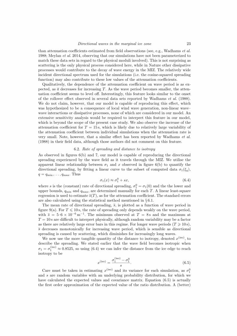
goodness of the least-square fit and the variability of the ensemble averaging process. Thestatistical method used to estimate the standard error is based on the random effectsmodel and the maximum likelihood method. It is described by Brockwell & Gordon(2001) in the context of medical science.Figure 8 shows the attenuation coefficient as a function of wave period, in the range T =

6 to 15 s. Note that the order of magnitude of a is O(10−6–10−5), which is slightly lower


than attenuation coefficients estimated from field observations (see, e.g., Wadhams et al.1988; Meylan et al. 2014, observing that our simulations have not been parameterized tomatch these data sets in regard to the physical moduli involved). This is not surprising asscattering is the only physical process considered here, while in Nature other dissipativeprocesses would contribute to the decay of wave energy in the MIZ. The relatively wideincident directional spectrum used for the simulations (i.e. the cosine-squared spreadingfunction) may also contribute to these low values of the attenuation coefficients.Qualitatively, the dependence of the attenuation coefficient on wave period is as ex-

pected, as a decreases for increasing T . As the wave period becomes smaller, the atten-uation coefficient seems to level off. Interestingly, this feature looks similar to the onsetof the rollover effect observed in several data sets reported by Wadhams et al. (1988).We do not claim, however, that our model is capable of reproducing this effect, whichwas hypothesized to be a consequence of local wind wave generation, non-linear wave–wave interactions or dissipative processes, none of which are considered in our model. Anextensive sensitivity analysis would be required to interpret this feature in our model,which is beyond the scope of the present case study. We also observe the increase of theattenuation coefficient for T = 15 s, which is likely due to relatively large variability ofthe attenuation coefficient between individual simulations when the attenuation rate isvery small. Note, however, that a similar effect has been reported by Wadhams et al.(1988) in their field data, although those authors did not comment on this feature.

6.2. Rate of spreading and distance to isotropy

As observed in figures 6(b) and 7, our model is capable of reproducing the directionalspreading experienced by the wave field as it travels through the MIZ. We utilise theapparent linear relationship between σ1 and x observed in figure 6(b) to quantify thedirectional spreading, by fitting a linear curve to the subset of computed data σ1(ξq),q = qmin, . . . , qmax. Thus

σ1(x) ≈ σ01 + sx, (6.4)

where s is the (constant) rate of directional spreading, σ01 = σ1(0) and the the lower and

upper bounds, qmin and qmax, are determined manually for each T . A linear least-squareregression is used to estimate s(T ), as for the attenuation coefficient. The standard errorsare also calculated using the statistical method mentioned in § 6.1.The mean rate of directional spreading, s, is plotted as a function of wave period in

figure 9(a). For T ⩽ 10 s, the rate of spreading only depends weakly on the wave period,with s = 5–6 × 10−6 m−1. The minimum observed at T = 8 s and the maximum atT = 10 s are difficult to interpret physically, although random variability may be a factoras there are relatively large error bars in this regime. For longer wave periods (T ⩾ 10 s),s decreases monotonically for increasing wave period, which is sensible as directionalspreading is caused by scattering, which diminishes for increasingly long waves.We now use the more tangible quantity of the distance to isotropy, denoted x(iso), to

describe the spreading. We stated earlier that the wave field becomes isotropic when

σ1 = σ(iso)1 ≈ 0.8525, so using (6.4) we can infer the distance from the ice edge to reach

isotropy to be

x(iso) =σ(iso)1 − σ0

1

s. (6.5)

Care must be taken in estimating x(iso) and its variance for each simulation, as σ01

and s are random variables with an underlying probability distribution, for which wehave calculated the expected values and covariance matrix. Equation (6.5) is actuallythe first order approximation of the expected value of the ratio distribution. A (better)


6 7 8 9 10 11 12 13 14 150

1

2

3

4

5

6

7x 10

−6

6 7 8 9 10 11 12 13 14 150

50

100

150

200

Figure 9. (a) Rate of directional spreading s as a function of wave period T in the range

6–15 s. (b) Distance to isotropy x(iso) plotted over the same range of wave periods. Error barsare computed as in figure 8.

second-order formula for estimating the expected value of the distance to isotropy isgiven by

x(iso) ≈ σ(iso)1 − σ0

1

s−

Cov(σ01 , s)

s2+

Var (s)(σ(iso)1 − σ0

1

)s3

, (6.6)

where Var and Cov denote the variance and covariance of random variables, respectively(see, e.g., Stuart & Ord 1999). A first-order formula can also be derived for the varianceof x(iso), i.e.

Var(x(iso)

)≈

(σ(iso)1 − σ0

1

s

)2 Var (s)(

σ(iso)1 − σ0

1

)2 − 2Cov

(σ01 , s)(

σ(iso)1 − σ0

1

)s+

Var(σ01

)s2

. (6.7)

Figure 9(b) depicts the expected value of the distance to isotropy x(iso) against waveperiod. The transition between the low-period and high-period regimes is clearly observedhere. Isotropy is reached within the first 40 km of the simulated MIZ for T ⩽ 10 s and

x(iso) varies little with T in this regime. On the other hand, x(iso) increases abruptly forT ⩾ 11 s, where the wave field spreads very slowly towards isotropy. For T > 12 s, values

of x(iso) greater than 500 km are computed, suggesting that long waves experience next tono spreading within the extent of a typical MIZ, i.e. over O(10–100) km. The transitionbetween the two regimes correlates with the prescribed maximum floe diameter of 200m,which is the open water wavelength of an 11.3 s wave. This finding suggests that waveslonger than the maximum floe size do not experience significant directional spreading inthe MIZ, which agrees with the observations of Wadhams et al. (1986).

7. Conclusion

In this paper we have devised a linear three-dimensional model of ocean wave atten-uation and directional spreading in the MIZ, governed by conservative scattering effectsalone. The simulated MIZ is composed of a large random array of floating ice floes,modelled as circular thin elastic plates. A random sea state with prescribed directional


spreading function defines the wave forcing. The solution to the scattering problem wasobtained using an extended version of the slab-clustering method, recently developed bythe authors in the context of acoustic wave scattering (see Montiel et al. 2015a), which inthis case accounts for evanescent vertical modes generated at each floe edge. This allowsus to (i) solve the deterministic multiple scattering of directional wave spectra by thou-sands to tens of thousands of floes for a manageable computation cost, (ii) simulate thepropagation of random sea states in randomly generated arrays of ice floes, and (iii) trackthe evolution of the wave field directional properties through the array.

Numerical convergence tests were conducted, with the key findings that:

(i) evanescent wave modes have little effect on the multiple scattering solution, even fork0a as large as O(10), and tightly packed arrays, suggesting the far-field approximationthat neglects these modes is valid for a wide range of parameters; and

(ii) a small proportion of the complex branches of the directional domain accuratelycaptures wave interactions between slabs.

Ensemble averaging was used to extract the attenuation and directional spreadingproperties of realistic random sea states through a random array of ice floes that resemblesa real MIZ. Randomness was included in the wave forcing, as an incoherent and ergodicdirectional sea state with a prescribed energy spreading function. Random arrays of icefloes were produced, with floe sizes drawn from an empirical power-law FSD. An analysisof these random features and the ensemble averaging process was conducted to identifypotential sources of computational savings. It was shown that

(i) a small number, i.e. O(1), of unique floe sizes only need to be considered in theFSD, thereby reducing the number of single-floe solutions to compute;

(ii) for each wave period a critical floe size can be defined, such that smaller floes havenegligible effect on the scattering properties of an array, suggesting that the smallest floescan be removed from the array. The critical floe size was found to be similar to the openwater wavelength. This reduces the number of floes in each slab and, concomitantly, thecomputational cost of solving the single-slab problem;

(iii) a small number of unique slabs (less than 10) need only be considered to generatelarge multiple slab arrays by taking random permutations of the unique slabs, reducingthe number of single-slab solutions to compute; and

(iv) introducing randomness in the array and the directional forcing reduces the vari-ability of the solution, so that a small number (e.g. 10) of random realizations of the arrayand forcing are required to obtain less than 1% relative standard error on the solution.

The method to extract wave energy attenuation and directional spreading in largerandom arrays was presented for a 50 km×50 km simulated MIZ (composed of 220 slabs).A directional energy density function was defined at each slab boundary to characterizethe directional content of wave energy there. Total wave energy is then obtained byintegrating the density over the directional range, while the directional spread is definedas the standard deviation of the normalised density interpreted as a probability densityfunction. The profile of wave energy and directional spread were then plotted for a numberof wave periods and analysed. The key findings of this analysis are summarised below.

(i) Wave energy profiles at mid-range and long wave periods showed clear trends ofexponential decay, which is consistent with field observations. A more complicated three-regime attenuation profile was observed at the lower end of the range of wave periods,likely due to the limited extent of the array.


(ii) The directional spread increases linearly with distance from the ice edge, until itreaches an isotropic state. For short wave periods, the limited extent of the array causesthe directional spread to take values higher than that for theoretical isotropy near theend of the simulated MIZ, as the directional energy density becomes distorted.

(iii) Fitting an exponential decay model to the wave energy profile at each wave period,we estimated the attenuation coefficient of wave energy, which is the most importantquantity parameterizing wave–sea ice interactions in large scale operational models. Ourestimates were found to be slightly smaller than those obtained from field observations,which is sensible recalling the other mechanisms of wave energy attenuations that areknown to exist in MIZs.

(iv) Fitting a linear growth model to the directional spread profile, we estimated therate of directional spreading (slope of linear model) and the distance from the ice edgeto reach isotropy. It was shown that two regimes of spreading exist. For short waveperiods, significant spreading is observed, although the amount of spreading experiencedvaries little with wave period. For long wave periods, the degree of directional spreadingdiminishes for increasing wave periods. The transition between the two regimes was foundto occur when the wavelength becomes larger than the maximum floe size.

FM and VAS are supported by the United States Office of Naval Research Departmen-tal Research Initiative ‘Sea State and Boundary Layer Physics of the Emerging ArcticOcean’ (Award number N00014-131-0279), EU FP7 Grant SPA-2013.1.1-06, and theUniversity of Otago. LGB is supported by an Australian Research Council DiscoveryEarly Career Researcher Award (DE13010157), the Australian Antarctic Science Pro-gram (Project 4123) and by the University of Adelaide. The authors are grateful toDavid Fletcher for helpful statistical mentorship.

Appendix A. Ergodicity of random directional sea states

Jefferys (1987) demonstrated that unrealistic standing wave patterns develop whensimulating single realizations of the random sea state (5.1). This is due to coherentinterference between wave components of the same frequency at different angles, which isreferred to as the phase locking phenomenon. This was also shown to be independent fromthe number of wave directions Ntr chosen to simulate the sea state. As a consequence,the sea state is not ergodic, which can be verified by expressing the time average of thewave energy as the autocorrelation of the signal (5.1) evaluated at the origin (see Ochi1998), i.e.

P =1

2

Ntr∑i=1

a2i +1

2

Ntr∑i=1

Ntr∑j=1, j =i

aiaj cosAij(x, y), (A 1)

where

Aij(x, y) = k0(x(cos τj − cos τi) + y(sin τj − sin τi)) + εj − εi.

The first term in (A 1) corresponds to the target mean energy of the incident spec-trum, which we seek to generate uniformly over the domain. The second term containsall interactions between waves travelling at different angles and depends on the spacevariables, so the wave energy is not uniform and the sea state is not ergodic. The targetmean energy can be partially recovered by taking an ensemble average over many ran-dom realizations of the sea state (5.1). The wave energy error then decays as the squareroot of the sample size (a property of ensemble averaging) with the second term in (A 1)averaging out to zero.


In practice, the uniformity of the wave energy in the spatial domain (i.e. the ergodicitycondition) can only be approximated by averaging over a sufficient number of realiza-tions. We perform Monte-Carlo simulations to analyze the variability of the mean energy(A 1) at the origin. We simulate a monochromatic sea state with period T = 9 s andenergy spreading function given by (5.2), recalling that no ice cover is present for thesesimulations. Simulating (5.2) for 1000 realizations of the sea state (5.1) evaluated at(x, y) = (0, 0), we find the 95% confidence interval for estimating the mean wave energyP is 0.06 < P < 3.7 with expected value 1, accounting for the fact that P is exponen-tially distributed (Jefferys 1987). This shows the significant variability of the mean waveenergy on the random variable of the sea state model. The variability can be reducedby averaging over a sample of mean energy estimates. We generate a new distribution ofmean energy P by estimating (A 1) at different locations of the open ocean, where eachmean is obtained by averaging over 50 realizations of the sea state. Invoking the centrallimit theorem, the distribution of P is normal, with 95% confidence interval P ≈ 1±0.28.This theoretical result was confirmed by numerical experiments.

We extend the analysis by estimating the error on the mean energy introduced bythe ensemble averaging method to approximate ergodicity. Using the 1000 simulated seastates generated earlier, we estimate the relative standard error of the mean energy on asingle realization of the sea state to be ≈ 100%. On the other hand, the relative standarderror of the mean energy estimated by averaging over 50 random realizations of the seastate is reduced ≈ 14%. From the slow convergence property of Monte Carlo simulations,we estimate that it would take approximately 10000 simulations to reduce further therelative error to 1%.

Appendix B. Random array generator

We generate the FSD in a given slab using a binning approach, whereby a small numberof floe radii (or bins) is considered, henceforth reducing the number of single floe solutionsto compute. The inputs of the procedure are the dimensions of the ice-covered region inthe slab, i.e. the width Lx and breadth Ly, the number of bins Nb, the ice concentrationc, the minimum and maximum floe radii amin and amax, and the exponent in the powerlaw distribution κ. Given these parameters, we determine the number of floes Ni withradius ai, for 1 ⩽ i ⩽ Nb and randomly position each floe in the slab using a circlepacking algorithm. The algorithm is outlined here:

1. define uniformly distributed bins ai, 1 ⩽ i ⩽ Nb, with a1 = amin and aNb= amax;

2. compute proportionality constants for each bin

λi =a1−κi+1 − a1−κ

i

a1−κmax − a1−κ

min

;

3. compute the total number of floes in the slab

Nf =

⌈cLxLy

π∑Nb

i=1 λia2i

⌉;

4. compute the number of floes in each bin

Ni = ⌈λiNf⌉;


5. adjust the ice-covered domain dimensions to obtain the desired ice concentration

L =π∑Nb

i=1 Nia2i

cLy;

6. position each floe iteratively at random in the ice-covered domain, such that floe/floeboundaries and floe/domain boundaries do not intersect (circle packing algorithm).

In step 2, we have defined ai = (ai−1+ai)/2, 2 ⩽ i ⩽ Nb−1, with a1 = a1 and aNb= aNb

.In steps 3 and 4, ⌈.⌉ denotes the ceiling function, which then introduces a discrepancy inthe concentration of ice floes. Step 5 adjusts the width of the domain to generate an FSDwith concentration as specified in the inputs. In step 6, floes are positioned in the domainiteratively in decreasing order of sizes, allowing us to reach higher concentrations.

REFERENCES

Abramowitz, M. & Stegun, I. A. 1970 Handbook of Mathematical Functions: with Formulas,Graphs, and Mathematical Tables. New York: Dover.

Bennetts, LG & Williams, TD 2015 Water wave transmission by an array of floating discs.Proc. R. Soc. Lond. A 471 (2173), 20140698.

Bennetts, L. G. 2011 Wave attenuation through multiple rows of scatterers with differingperiodicities. SIAM J. Appl. Math. 71, 540–558.

Bennetts, L. G., Alberello, A., Meylan, M. H., Cavaliere, C., Babanin, A. V. &Toffoli, A. 2015 An idealised experimental model of ocean surface wave transmission byan ice floe. Ocean Model. p. doi:10.1016/j.ocemod.2015.03.001.

Bennetts, L. G., Peter, M. A., Squire, V. A. & Meylan, M. H. 2010 A three dimensionalmodel of wave attenuation in the marginal ice zone. J. Geophys. Res. 115, C12043.

Bennetts, L. G. & Squire, V. A. 2009 Wave scattering by multiple rows of circular ice floes.J. Fluid Mech. 639, 213–238.

Bennetts, L. G. & Squire, V. A. 2012a Model sensitivity analysis of scattering-inducedattenuation of ice-coupled waves. Ocean Model. 45, 1–13.

Bennetts, L. G. & Squire, V. A. 2012b On the calculation of an attenuation coefficient fortransects of ice-covered ocean. Proc. R. Soc. Lond. A 468, 136–162.

Brockwell, S. E. & Gordon, I. R. 2001 A comparison of statistical methods for meta-analysis. Stat. Med. 20 (6), 825–840.

Collins, C. O., Rogers, W. E., Marchenko, A. & Babanin, A. V. 2015 In situ measure-ments of an energetic wave event in the arctic marginal ice zone. Geophys. Res. Lett. 42 (6),1863–1870.

Doble, M. J. & Bidlot, J.-R. 2013 Wave buoy measurements at the Antarctic sea ice edgecompared with an enhanced ECMWF WAM: progress towards global waves-in-ice mod-elling. Ocean Model. 70, 166–173.

Dumont, D., Kohout, A. L. & Bertino, L. 2011 A wave-based model for the marginal icezone including a floe breaking parameterization. J. Geophys. Res. 116, C04001.

Ishimaru, A. 1978 Wave Propagation and Scattering in Random Media. Academic Press, NewYork.

Jefferys, E. R. 1987 Directional seas should be ergodic. Appl. Ocean Res. 9, 186–191.Kagemoto, H. & Yue, D. K. P. 1986 Interactions among multiple three-dimensional bodies

in water waves: an exact algebraic method. J. Fluid Mech. 166, 189–209.Kohout, A. L. & Meylan, M. H. 2008 An elastic plate model for wave attenuation and ice

floe breaking in the marginal ice zone. J. Geophys. Res. 113, C09016.Kohout, A. L., Williams, M. J. M., Dean, S. M. & Meylan, M. H. 2014 Storm-induced

sea-ice breakup and the implications for ice extent. Nature 509 (7502), 604–607.Krogstad, H. E. 2005 The directional wave spectrum. In Measuring and Analysing the Direc-

tional Spectrum of Ocean Waves (ed. D. Hauser, K. Kahma, H. E. Krogstad, S. Lehner,J. A. J. Monbaliu & L. R. Wyatt), pp. 15–54. Cost Action 714, EUR 21367, Luxembourg:Office for Official Publications of the European Communities.


Laxon, S. W, Giles, K. A, Ridout, A. L, Wingham, D. J, Willatt, R., Cullen, R.,Kwok, R., Schweiger, A., Zhang, J., Haas, C. et al. 2013 Cryosat-2 estimates of Acticsea ice thicness and volume. Geophys. Res. Lett. 40 (4), 732–737.

Linton, C. M. & Evans, D. V. 1992 The radiation and scattering of surface waves by a verticalcircular cylinder in a channel. Philos. T. R. Soc. A 338, 325–357.

Liu, A. K., Holt, B. & Vachon, P. W. 1991a Wave propagation in the marginal ice zone:Model predictions and comparisons with buoy and synthetic aperture radar data. J. Geo-phys. Res. 96 (C3), 4605–4621.

Liu, A. K. & Mollo-Christensen, E. 1988 Wave propagation in a solid ice pack. J. Phys.Oceanogr. 18 (11), 1702–1712.

Liu, A. K., Vachon, P. W. & Peng, C. Y. 1991b Observation of wave refraction at an iceedge by synthetic aperture radar. J. Geophys. Res. 96 (C3), 4803–4808.

Martin, P. A. 2006 Multiple Scattering: Interaction of Time-Harmonic Waves with N Obsta-cles, Issue 107 of Encyclopedia of Mathematics and Its Applications, vol. 10. CambridgeUniversity Press.

Masson, D. & Leblond, P. H. 1989 Spectral evolution of wind-generated surface gravity wavesin a dispersed ice field. J. Fluid Mech. 202, 43–81.

Mavrakos, S. A. & Koumoutsakos, P. 1987 Hydrodynamic interaction among vertical ax-isymmetric bodies restrained in waves. Appl. Ocean Res. 9, 128–140.

Meier, W. N., Gallaher, D. & Campbell, G. G. 2013 New estimates of Arctic and Antarcticsea ice extent during September 1964 from recovered Nimbus I satellite imagery. Cryo. Disc.7, 35–53.

Mellor, M. 1986 Mechanical behavior of sea ice. In The Geophysics of Sea Ice (ed. N. Unter-steiner), pp. 165–281. NATO Advanced Study Institute Series.

Meylan, M. H., Bennetts, L. G. & Kohout, A. L. 2014 In situ measurements and analysisof ocean waves in the Antarctic marginal ice zone. Geophys. Res. Lett. 41 (14), 5046–5051.

Meylan, M. H. & Masson, D. 2006 A linear Boltzmann equation to model wave scatteringin the marginal ice zone. Ocean Model. 11, 417–427.

Meylan, M. H. & Squire, V. A. 1996 Response of a circular ice floe to ocean waves. J.Geophys. Res. 101, 8869–8884.

Meylan, M. H., Squire, V. A & Fox, C. 1997 Toward realism in modeling ocean wavebehavior in marginal ice zones. J. Geophys. Res 102, 22,981–22,991.

Miles, M. D. & Funke, E. R. 1989 A comparison of methods for synthesis of directional seas.J. Offshore Mech. Arct. Eng. 111 (1), 43–48.

Montiel, F. 2012 Numerical and experimental analysis of water wave scattering by floatingelastic plates. PhD thesis, University of Otago.

Montiel, F., Bennetts, L. G., Squire, V. A., Bonnefoy, F. & Ferrant, P. 2013 Hydroe-lastic response of floating elastic discs to regular waves. part 2. modal analysis. J. FluidMech. 723, 629–652.

Montiel, F., Squire, V. A. & Bennetts, L. G. 2015a Evolution of directional wave spectrathrough finite regular and randomly perturbed arrays of scatterers. SIAM J. Appl. Math.75, 630–651.

Montiel, F., Squire, V. A. & Bennetts, L. G. 2015b Reflection and transmission of oceanwave spectra by a band of randomly distributed ice floes. Ann. Glaciol. 56(69), 315–322.

Mosig, J. E. M., Montiel, F. & Squire, V. A. 2015 Comparison of viscoelastic-type modelsfor ocean wave attenuation in ice-covered seas. J. Geophys. Res. 120.

Ochi, M. K. 1998 Ocean Waves: The Stochastic Approach. Cambridge University Press.Ohkusu, M. 1974 Hydrodynamic forces on multiple cylinders in waves. In Proceedings of the

International Symposium on the Dynamics of Marine Vehicles and Structures in Waves(ed. R. E. D. Bishop & W. G. Price).

Peter, M. A. & Meylan, M. H. 2004 Infinite-depth interaction theory for arbitrary floatingbodies applied to wave forcing on ice floes. J. Fluid Mech. 500, 145–167.

Peter, M. A. & Meylan, M. H. 2009 Water wave scattering by vast field of bodies. SIAM J.Appl. Math. 70, 1567–1586.

Peter, M. A., Meylan, M. H. & Chung, H. 2003 Wave scattering by a circular plate in waterof finite depth: a closed form solution. In Proceedings of the 13th International Offshoreand Polar Engineering Conference, pp. 180–185.


Robinson, N. J. & Palmer, S. C. 1990 A modal analysis of a rectangular plate floating on anincompressible liquid. J. Sound Vib. 142, 453–460.

Rogers, W. E. & Orzech, M. D. 2013 Implementation and testing of ice and mud sourcefunctions in WAVEWATCH IIIR⃝. Tech. Rep.. National Research Laboratory.

Rothrock, D. A. & Thorndike, A. S. 1984 Measuring the sea ice floe size distribution. J.Geophys. Res. Oceans 89 (C4), 6477–6486.

Shen, H. H. & Squire, V. A. 1998 Wave damping in compact pancake ice fields due tointeractions between pancakes. Antarctic Research Series 74, 325–341.

Skene, D. M., Bennetts, L. G., Meylan, M. H. & Toffoli, A. 2015 Modelling water waveoverwash of a thin floating plate. Journal of Fluid Mechanics 777, R3.

Sommerfeld, A. 1949 Partial Differential Equations in Physics, Pure and Applied Mathemat-ics: A Series of Monographs and Textbooks, vol. 1. Academic Press.

Squire, V. A. 2007 Of ocean waves and sea-ice revisited. Cold Reg. Sci. Technol. 49, 110–133.Squire, V. A. 2011 Past, present and impendent hydroelastic challenges in the polar and

subpolar seas. Philos. T. R. Soc. A 369, 2813–2831.Squire, V. A., Dugan, J. P., Wadhams, P., Rottier, P. J. & Liu, A. K. 1995 Of ocean

waves and sea ice. Annu. Rev. Fluid Mech. 27, 115–168.Squire, V. A. & Fox, C. 1992 On ice coupled waves: a comparison of data and theory. In

Advances in ice technology: Proc. 3rd Int. Conf. on Ice Technology , pp. 269–280.Squire, V. A. & Moore, S. C. 1980 Direct measurement of the attenuation of ocean waves

by pack ice. Nature 283, 365–368.Stuart, A. & Ord, K. 1999 Kendall’s Advanced Theory of Statistics. Volume 1: Distribution

Theory . Arnold.Thomson, J. & Rogers, W. E. 2014 Swell and sea in the emerging Arctic Ocean. Geophys.

Res. Lett. 41 (9), 3136–3140.Toyota, T., Haas, C. & Tamura, T. 2011 Size distribution and shape properties of relatively

small sea-ice floes in the Antarctic marginal ice zone in late winter. Deep-Sea Res Pt. II58, 1182–1193.

Toyota, T., Takatsuji, S. & Nakayama, M. 2006 Characteristics of sea ice floe size distri-bution in the seasonal ice zone. Geophys. Res. Lett. 33 (2), L02616.

Twersky, V. 1952 Multiple scattering of radiation by an arbitrary configuration of parallelcylinders. J. Acoust. Soc. Am. 24, 42–46.

Wadhams, P., Squire, V. A., Ewing, J. A. & Pascal, R. W. 1986 The effect of the marginalice zone on the directional wave spectrum of the ocean. J. Phys. Oceanogr. 16, 358–376.

Wadhams, P., Squire, V. A., Goodman, D. J., Cowan, A. M. & Moore, S. C. 1988 Theattenuation rates of ocean waves in the marginal ice zone. J. Geophys. Res. 93, 6799–6818.

Wang, R. & Shen, H. H. 2010 Gravity waves propagating into an ice-covered ocean: a vis-coelastic model. J. Geophys. Res. 115 (C6).

Williams, T. D., Bennetts, L. G., Squire, V. A., Dumont, D. & Bertino, L. 2013a Wave-ice interactions in the marginal ice zone. Part 1: Theoretical foundations. Ocean Model. 71,81–91.

Williams, T. D., Bennetts, L. G., Squire, V. A., Dumont, D. & Bertino, L. 2013b Wave-ice interactions in the marginal ice zone. Part 2: Numerical implementation and sensitivitystudies along 1D transects of the ocean surface. Ocean Model. 71, 92–101.

Young, I. R., Zieger, S. & Babanin, A. V. 2011 Global trends in wind speed and waveheight. Science 332 (6028), 451–455.

fabien montiel, v. a. squire, and l. g. bennetts ... · under consideration for publication in j....

Documents