fabio villone diei, universitàdi cassino, italy · nonlinear structural materials module pipe flow...

Fabio Villone

DIEI, Università di Cassino, Italy

HTS modelling 2016 1

Statement of the problem

A historical perspective

State of the art

Research directions Focus on fast methods

An example: fusion devices

Conclusions & outlook


I will present my personal view of the history, state of the art and research trends of low-frequency computational electromagnetics Others may have different opinions

I will focus on near-term future developments, basically extrapolating what is currently done No “fiction movie” effort


Something trivial to start with...


We deal with low-frequency electromagnetics No wave propagation

Frequency low enough For systems with dimensions ≈ 10 m, this means

frequencies below around 1 MHz

At least one of the time derivatives in Maxwell’s equation may be neglected Static and quasi-static models


c

LEMEM =<< ττω ,1

Among quasi-static models we deal with eddy currents model

Magneto-Quasi-Static Magnetic energy prevailing on electric energy

(Magnetic)

Low-frequency (Quasi-Static)


0=⋅∇=×∇

∂∂−=×∇

B

JH

BE

tinitial conditionsboundary conditionscontinuity conditionsmaterial properties

(Obviously...) of interest for HTS community Typical applications fall inside this classification

Peculiar with respect to full Maxwell model Distinct mathematical properties (parabolic vs.

hyperbolic)

Need for dedicated solvers and ad hoc analytical and numerical approaches

Much more difficult than Electro-Quasi-Static model


First problem: formulation Choice of the primary unknown in which the

problem must be recast

A “first choice” does not exist (not like EQS...)

Magnetic vs. Electric formulations Warning: electric field outside conductors

Fields vs. Potentials Warning: gauge conditions

Differential vs. Integral Fields or sources?


Second problem: the unknown quantities are intrinsically vectors Three components per point

Continuity conditions

Numerical difficulties “Naive” numerical approaches may be inadequate

Need for specific numerical treatment of eddy currents problem


A 40-year long story...


First applications of computers to calculation of magnetic fields

Computer = big calculator


Magnetostatic computations, from 2D to 3D


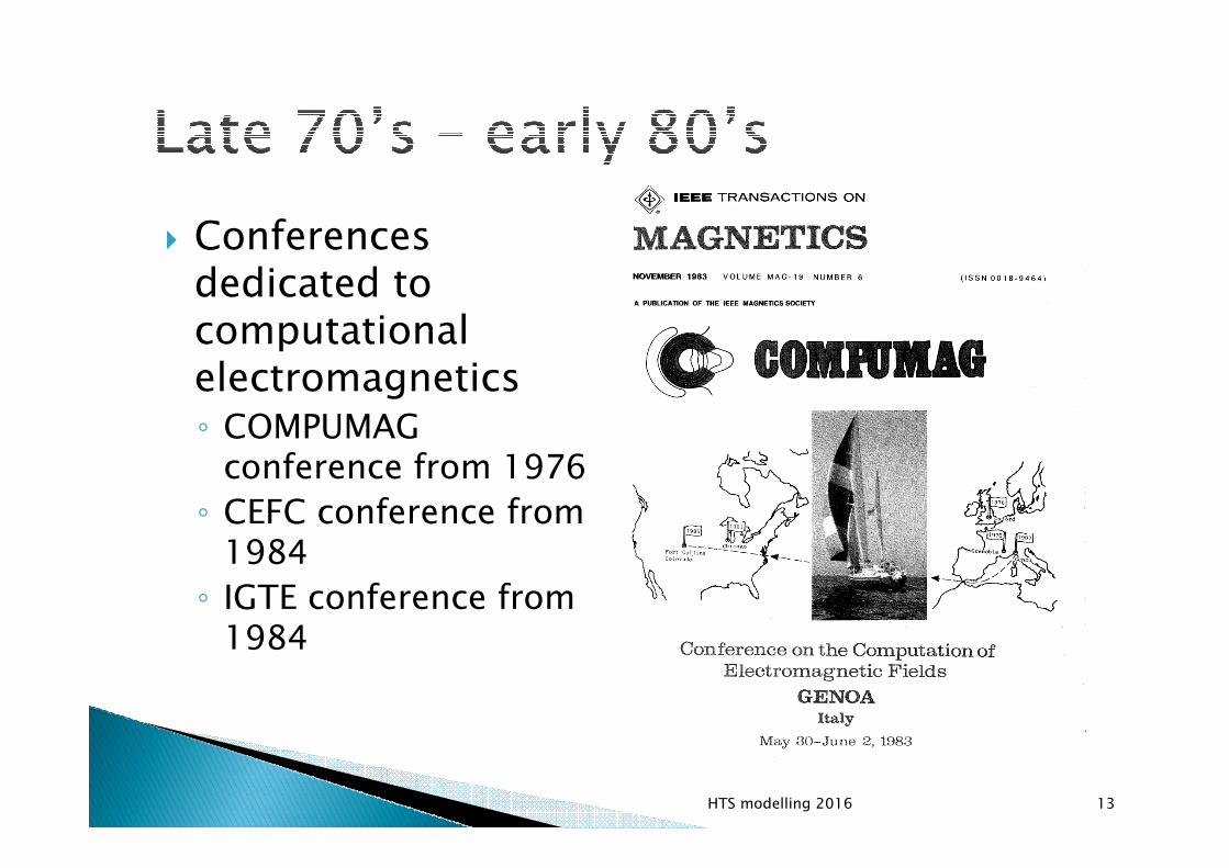
Conferences dedicated to computational electromagnetics COMPUMAG

conference from 1976

CEFC conference from 1984

IGTE conference from 1984


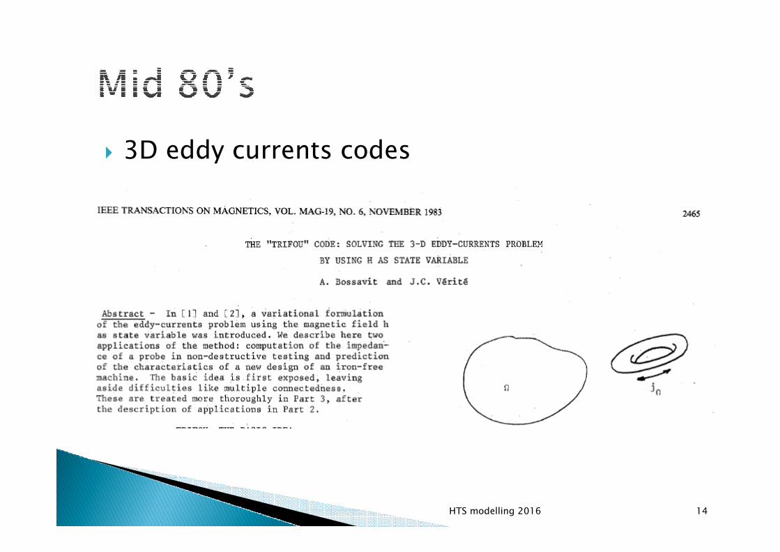
3D eddy currents codes


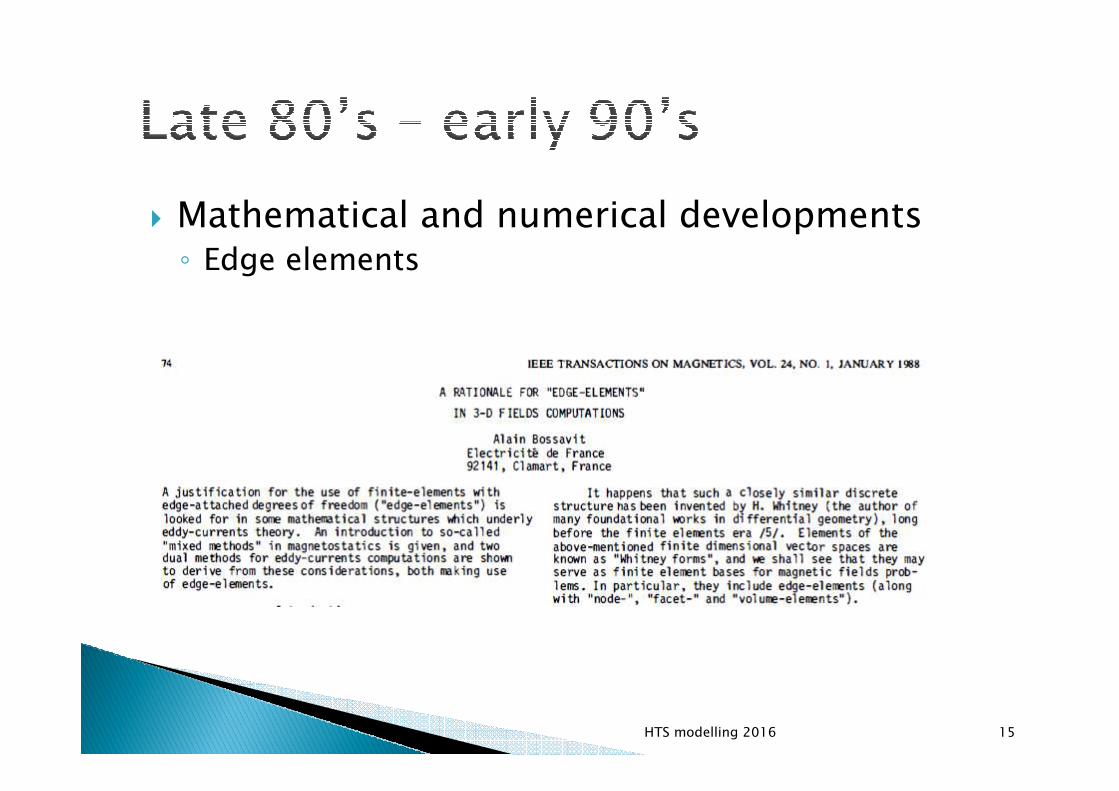
Mathematical and numerical developments Edge elements


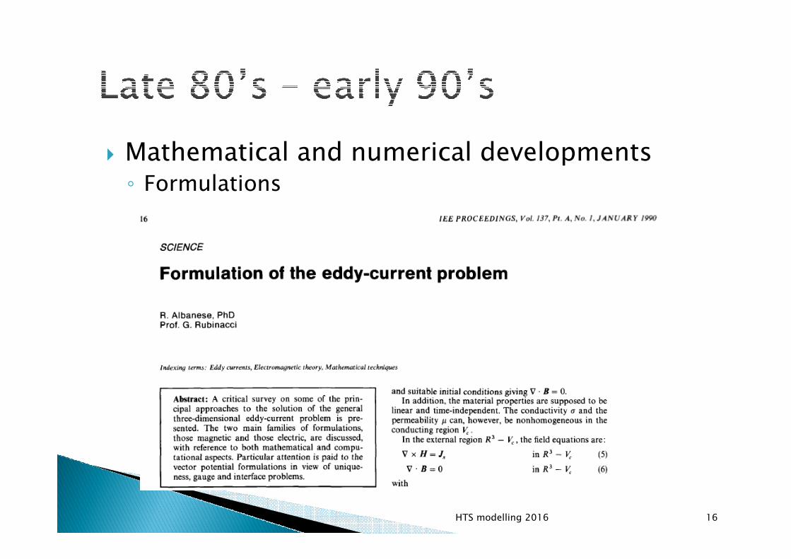
Mathematical and numerical developments Formulations


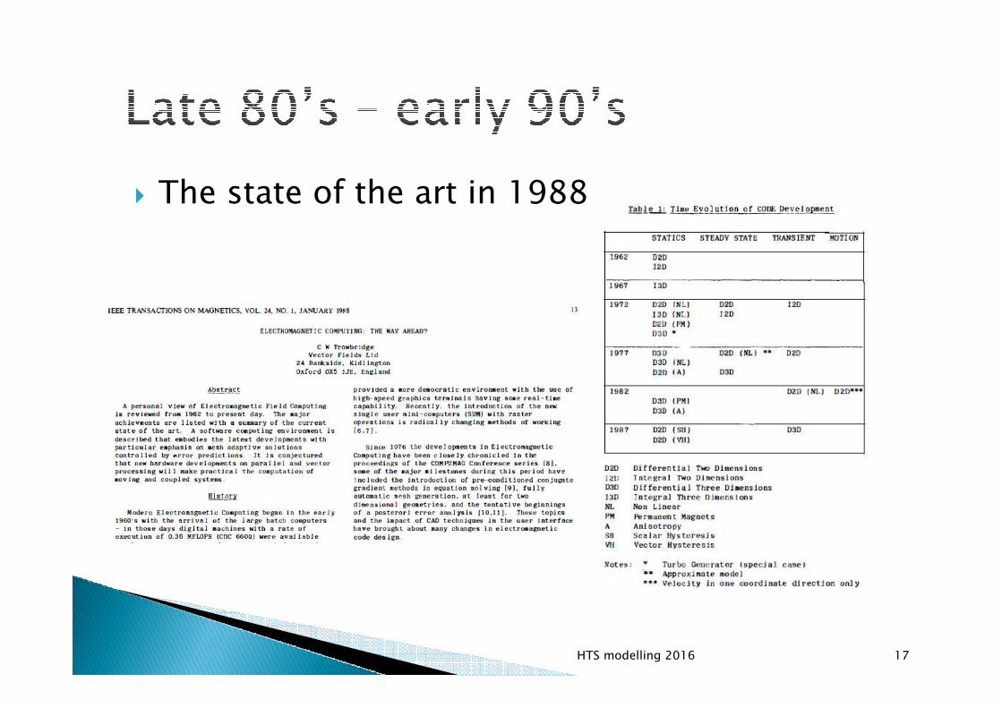
The state of the art in 1988


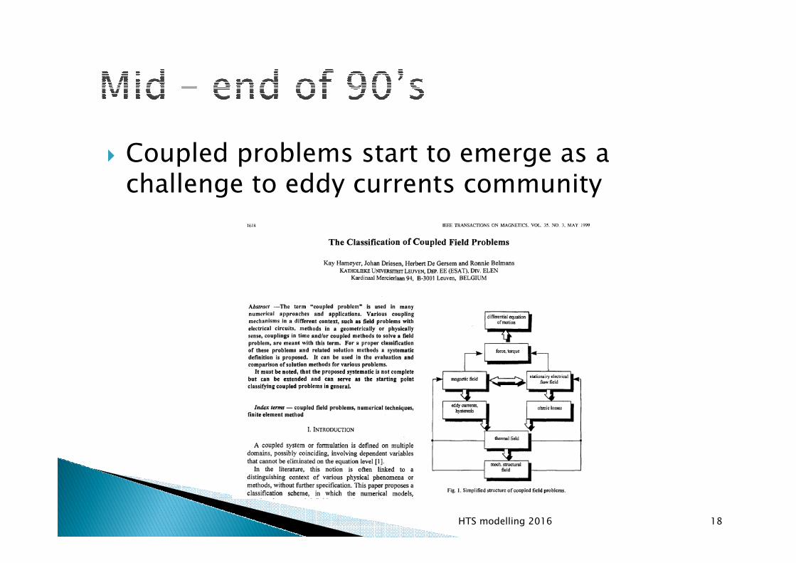
Coupled problems start to emerge as a challenge to eddy currents community


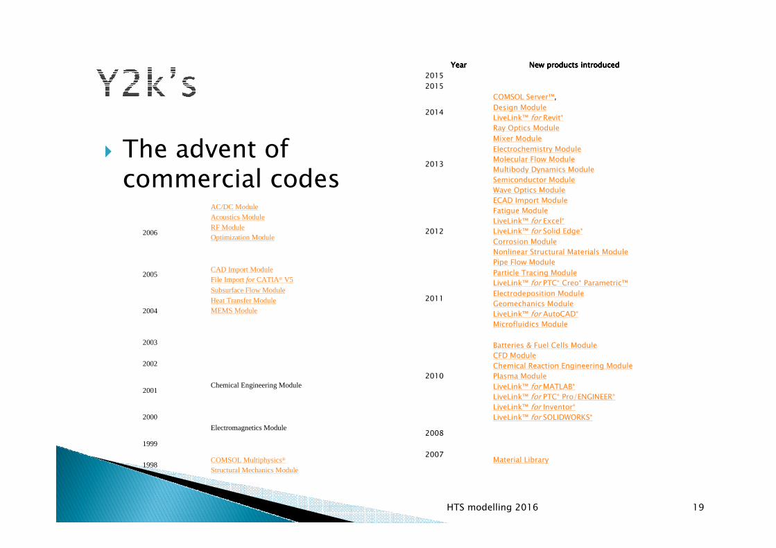
The advent of commercial codes


YearYearYearYear New products introducedNew products introducedNew products introducedNew products introduced

2015

2015

2014

COMSOL Server™,

Design Module

LiveLink™ for Revit®

Ray Optics Module

2013

Mixer Module

Electrochemistry Module

Molecular Flow Module

Multibody Dynamics Module

Semiconductor Module

Wave Optics Module

2012

ECAD Import Module

Fatigue Module

LiveLink™ for Excel®

LiveLink™ for Solid Edge®

Corrosion Module

Nonlinear Structural Materials Module

Pipe Flow Module

2011

Particle Tracing Module

LiveLink™ for PTC® Creo® Parametric™

Electrodeposition Module

Geomechanics Module

LiveLink™ for AutoCAD®

Microfluidics Module

2010

Batteries & Fuel Cells Module

CFD Module

Chemical Reaction Engineering Module

Plasma Module

LiveLink™ for MATLAB®

LiveLink™ for PTC® Pro/ENGINEER®

LiveLink™ for Inventor®

LiveLink™ for SOLIDWORKS®

2008

2007Material Library

2006

AC/DC ModuleAcoustics ModuleRF ModuleOptimization Module

2005CAD Import ModuleFile Importfor CATIA® V5

2004

Subsurface Flow ModuleHeat Transfer ModuleMEMS Module

2003

2002

2001Chemical Engineering Module

2000

Electromagnetics Module

1999

1998COMSOL Multiphysics®

Structural Mechanics Module

The advent of commercial codes


Being commercial codes quite advanced, the interest of the scientific community of low-frequency computational electromagnetics is diverting from “traditional paths”

Focus on: Specific applications out of reach of commercial

codes (e.g. advanced materials modelling)

Numerical techniques not (yet?) routinely available on commercial codes (e.g. fast techniques)


My personal view


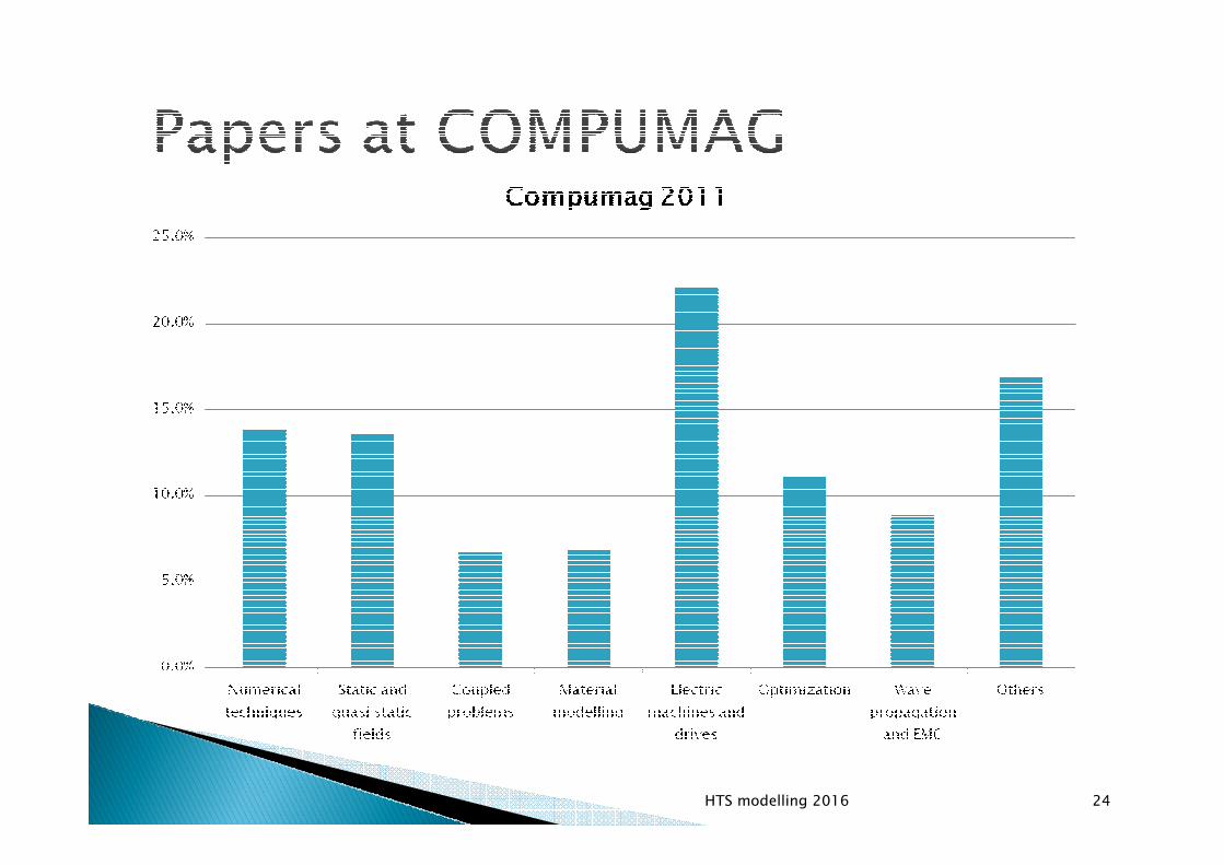
State of the art: what the community of low-frequency computational electromagnetics is currently doing

Let us as “proxy” of the state of the art the number of papers presented at the latest COMPUMAG conferences (2011,2013,2015) on each broad topic


Some general trends emerge Not of interest for HTS community ≈ 60% Electric machines ≈ 20% Optimization ≈ 15 % Wave propagation & EMC ≈ 10% Rest of the spectrum ≈ 15 %

Potential interest for HTS community ≈ 40% Numerical techniques Static & quasi-static fields Coupled problems Material modelling


My personal view


For each of the items of the state of the art of potential interest for HTS community, I provide my personal view of the research directions

Personal selection Most interesting topics (personal preference)

Most promising topics for computational electromagnetics

(Still) largely out of reach of commercial codes

Potential fall-out to HTS community


Fast methods for large-scale problems Domain decomposition

Compression

Multipoles

Model order reduction

Parallelization on multiple CPUs

GPUs and High Performance Computing

Numerical advances Meshless method / radial basis functions

Discontinuous / moving meshes

Gauging/preconditioning/convergence


Numerical analysis of low-frequency systems Inductance and capacitance calculations

Shielding

New methods/formulations (very few...)

Force computations


Multiphysics problems EM + circuits (interconnections etc.)

EM + mechanics (motors, vibrations etc.)

EM + thermal (induction heating etc.)

EM + fluid (gas, plasmas etc.)

Commercial codes are catching up...


Magnetic materials Hysteresis Micromagnetics

“New” materials Anisotropic / layered materials Metamaterials Graphene et similia

Homogenization & multiscale Superconductors Quench, losses etc. Materials & devices


A few examples


Integral formulations of the eddy currents problem require the storage of matrices of size scaling as N2 (N being the number of discrete unknowns), and their inversion needs a computational cost of the order of N3, if a direct solver is used May get impractically high for detailed meshes

Drives towards iterative inversion schemes

Need to improve the computational scaling, i.e. the dependence on N of the computational cost


Key ingredients (assuming iterative inversion methods) Preconditioning of matrix to be inverted

(less iterations needed)

Fast matrix-vector product (less computations per iteration)

Parallelization


Rationale: a lower condition number means less iterations of iterative methods

Mathematically: such that P-1A has a lower condition number than A

Practically: find an “easy to invert” matrix P (e.g. quasi-diagonal) sufficiently “close” to original matrix so that P-1A gets “close to identity”


( ) bPxAPbxA 11 −− =⇒=

Matrix – vector product often has a clear physical meaning Magnetic field produced by a given source

Fast Fourier Transform (FFT) Equivalent sources on suitable regular grids Matrix-vector product can be accelerated by means of a

fast convolution product

Fast Multipole Method (FMM) If the field point is far enough, the electromagnetic field

source can be characterized by few parameters (multipoles) The sources are expanded in spherical harmonics and

the field computation takes into account a limited number of such harmonics


Singular Value Decomposition (SVD) Physically: the magnetic field produced by a set of

sources grouped in a given region VS, when evaluated in a different region VE, can be described through a linear operator having a rank r decreasing as the relative separation between VS and VE is increased.

Mathematically: low rank QR factorization of original matrix (e.g. through Gram-Schmidt)


Nr

NrRrNQNNA

xRyyQxQRxA

<<×××

==≈:,:,:

,


Location of magnetic field sources

Close region (no approximation)

Far regions (low-rank approximation)

A more complicated example...


The overall performance can be quite satisfactory


Computational time scaling almost linearly with N

Speed-up with respect to standard calculations

Multiple CPUs Standard libraries support parallelization on CPUs

Which are the factors to be taken into account? Assembly balancing: the computational times for the

matrix assembly should be balanced among the processor Memory balancing: local memory required to store each

part of the matrix should be equally distributed among processors Computational balancing: computational time to build

matrix-vector product should be balanced among processors

Solving this optimal allocation problem has an exponential complexity sub-optimal algorithms required


GPUs Design philosophy tailored on the inherently parallel

nature of graphics rendering Large amount of cores in order to execute a large

number of execution threads at the same time Massive multithreading (up to thousands cores), small

cache memory with very simple control unit Each computational thread performs roughly same task

onto different partitions of data The code needs to be split into the sequential parts

(on the CPU) and the numerically intensive (on the GPUs) GPUs complement CPU execution Reprogramming of codes needed


My favourite topic...


Nuclear fusion claims to be one possible option for future energy needs of mankind: the fusion of nuclei of light elements (H or isotopes), to give heavier elements (e.g He), produces net energy thanks to mass defect

Thermonuclear fusion: electrostatic repulsion is overcome by increasing the temperature of the gas (hundreds of millions °C) ⇒ plasma (fully ionized gas)

Magnetic confinement: suitable magnetic fields give shape to plasma and prevent it from hitting the surrounding walls

Tokamak: toroidal device to avoid plasma losses at ends


Multiphysics Electromagnetic interaction plasma-conductors

Nonlinear Plasma behaviour

Large scale Large devices with fine geometrical details

Free boundary Plasma/vacuum interface not defined a priori

Force computation Currents-fields interactions on plasma and on structures

Superconducting coils Not treated in the following...


Coupling surface to describe the electromagnetic interaction between the plasma and the conductors

Different formulations in each domain the best choice in each region

Can be generalized to other multiphysics problems


Inside Ω: Grad-Shafranov equations(elliptic nonlinear problem)

Outside Ω: eddy currents in 3D structures (parabolic linear problem)

On ∂Ω: coupling conditions


Inside Ω: Magneto-Hydro-Dynamics (MHD) eqns.

If the time scale is slow enough: neglect plasma mass Plasma mass plays a role only on µs time scale Plasma evolves instantaneously through equilibrium states

(evolutionary equilibrium)

If the plasma evolution is around an equilibrium point: linearization

mass balance

momentum balance

energy balance (adiabatic)

Grad-Shafranov nonlinear elliptic equation

Differential formulation in weak form

2ndorder triangular finite elements

Overall system:


ψ : poloidal magnetic fluxjϕ(ψ): plasma current density (nonlin. funct. of ψ)boundary value: coupling conditions

Outside Ω: eddy currents (linear parabolic)

Integral formulation in terms of JJJJ in weak form

Electric vector potential with two-component gauge

Volumetric finite elements (hexa, tetra,…)

Edge elements:


Linear nonmagnetic conductors

Dynamical eqns solved with implicit time stepping

Equivalent currents located on the coupling surface, producing the same magnetic field as plasmaoutside the coupling surface Proportional to plasma current density

Coupled to 3D structures via mutual inductance

Overall discrete equations:


Flux induced by plasma current on 3D structures

Coupling condition on poloidal flux :

Plasma contribution: Proportional to plasma current density

External contribution: Proportional to 3D currents (Biot-Savart)

Combining everything, at each time step we have:


Nonlinear set of Ni

equations (as many as nodes in 2D triangular mesh inside Ω), solved with Newton-Raphson method

“ITER is a large-scale scientific experiment that aims to demonstrate that it is possible to produce commercial energy from fusion”

Currently being built in France by seven international partners (EU, USA, Japan, China, India, Korea, Russia)

Multi-billionaire budget


Study of off-normal plasma events (disruptions), consisting of a rapid loss (<100 ms) of thermal and magnetic plasma energy

Eddy currents induced in conducting structures

Current – field interaction give rise to electromagnetic forces which may put at risk the integrity of the machine

Movie of disruption simulation


The Experimental Advanced Superconducting Tokamak (EAST) is an experimental device with fully superconducting poloidal and toroidal coils

Designed and constructed to explore the physical and engineering issues under steady state operation for support of future fusion reactors

EAST has recently undertaken an extensive upgrade ⇒ modelling need


EAST is an intrinsic 3D device The axisymmetric conducting structures are “too

far” from plasma

Need for a detailed 3D modelling


Complicated 3D eddy current density patterns induced in conducting structures


3D effects are fundamental in providing a correct prediction of experimental results


Finally at the end...


Low-frequency computational electromagnetics: a 40-year long story

Tumultuous and fast advances for the first 20 years or so

Now it can be considered a more “mature”sector Advent of commercial codes, which can treat

routinely “standard” applications The interests of the scientific community are

diverting WARNING: need for awareness of use of commercial

codes!!


New research trends are emerging Focus on topics/techniques still out of reach of

commercial codes...

... shifting to commercial applications in the near future?

Several new research directions may be of interest for the HTS community Fast methods, force computations, multiscale,

multiphysics etc.



“Παντα ρει, και ουδεν µενει”

“Everything flows, nothing stands still”

Heraclitus, around 500 BC

fabio villone diei, universitàdi cassino, italy · nonlinear structural materials module pipe flow...

Documents