Face Recognition

CSE 576

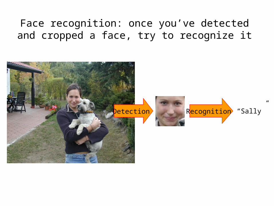
Face recognition: once you’ve detected and cropped a face, try to recognize it

Detection Recognition “Sally”

Face recognition: overview• Typical scenario: few examples per face,

identify or verify test example• What’s hard: changes in expression,

lighting, age, occlusion, viewpoint• Basic approaches (all nearest neighbor)

1. Project into a new subspace2. Measure face features

Typical face recognition scenarios

• Verification: a person is claiming a particular identity; verify whether that is true– E.g., security

• Closed-world identification: assign a face to one person from among a known set

• General identification: assign a face to a known person or to “unknown”

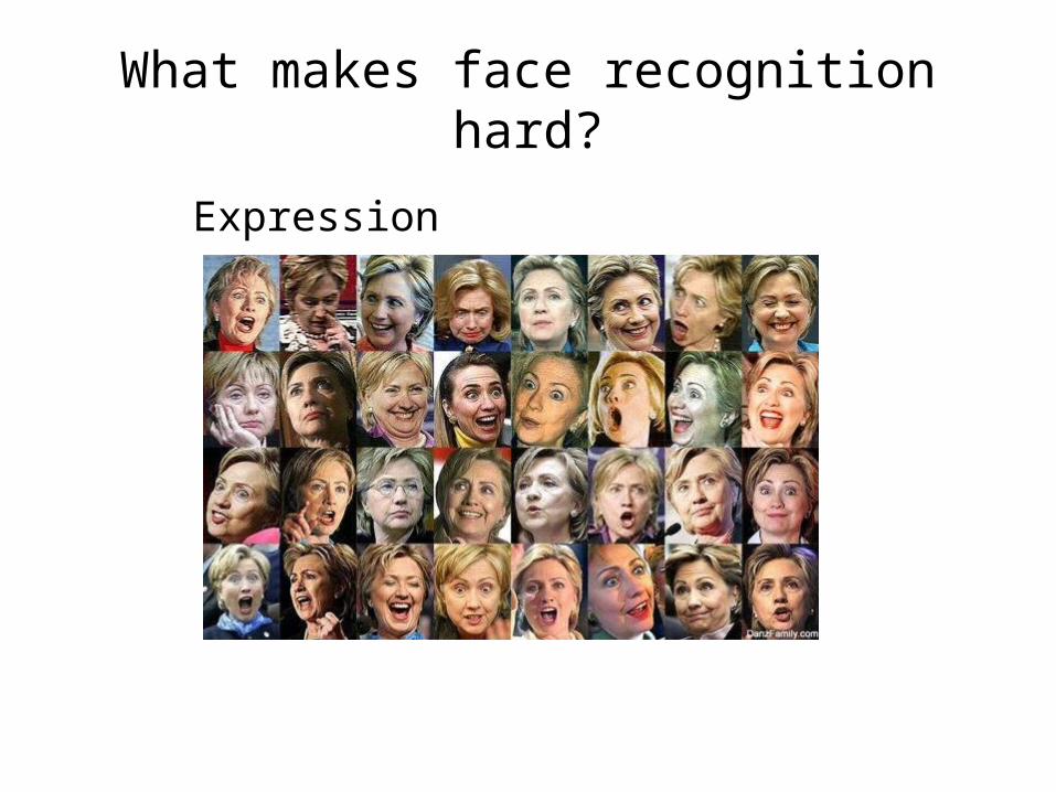
What makes face recognition hard?

Expression

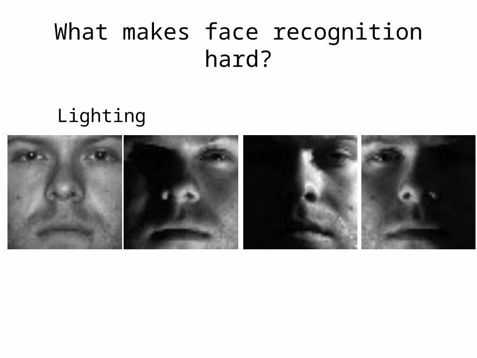
What makes face recognition hard?

Lighting

What makes face recognition hard?

Occlusion

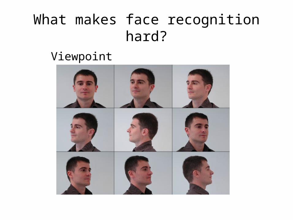
What makes face recognition hard?Viewpoint

Simple idea for face recognition1. Treat face image as a vector of intensities

2. Recognize face by nearest neighbor in database

x

nyy ...1

xy kk

k argmin

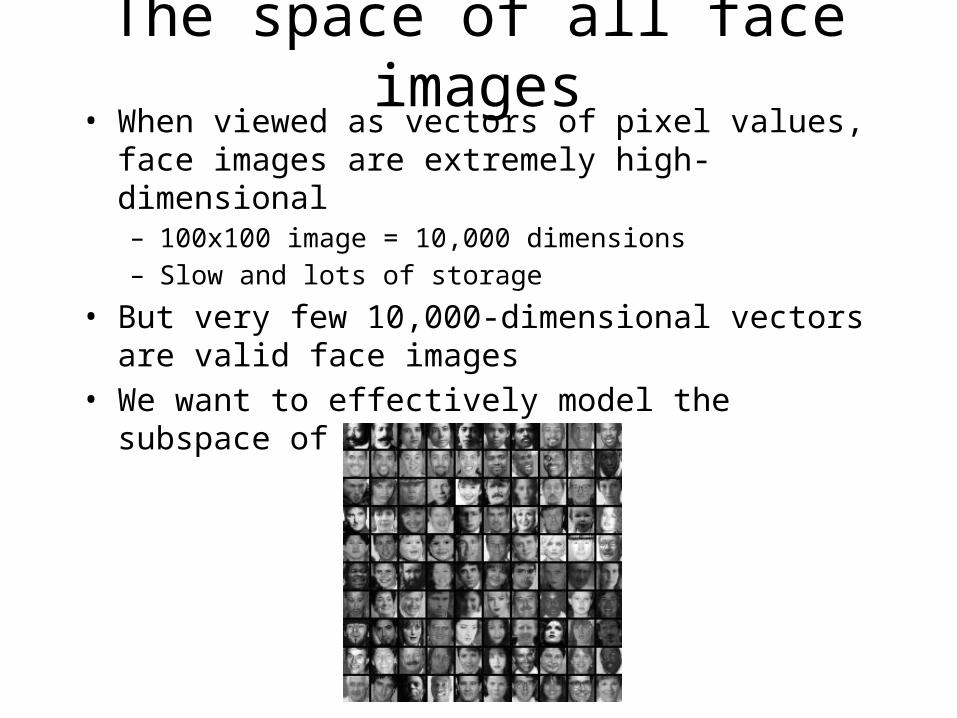
The space of all face images• When viewed as vectors of pixel values, face images are

extremely high-dimensional– 100x100 image = 10,000 dimensions– Slow and lots of storage

• But very few 10,000-dimensional vectors are valid face images

• We want to effectively model the subspace of face images

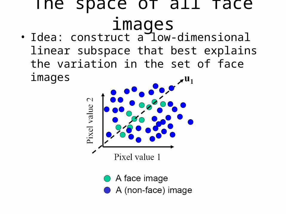
The space of all face images• Idea: construct a low-dimensional linear subspace

that best explains the variation in the set of face images

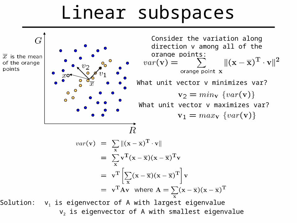
Linear subspacesConsider the variation along direction v among all of the orange points:

What unit vector v minimizes var?

What unit vector v maximizes var?

Solution: v1 is eigenvector of A with largest eigenvalue v2 is eigenvector of A with smallest eigenvalue

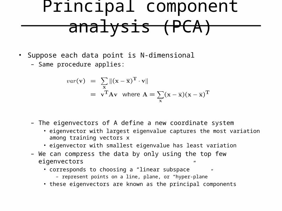
Principal component analysis (PCA)

• Suppose each data point is N-dimensional– Same procedure applies:

– The eigenvectors of A define a new coordinate system• eigenvector with largest eigenvalue captures the most variation among training

vectors x• eigenvector with smallest eigenvalue has least variation

– We can compress the data by only using the top few eigenvectors• corresponds to choosing a “linear subspace”

– represent points on a line, plane, or “hyper-plane”

• these eigenvectors are known as the principal components

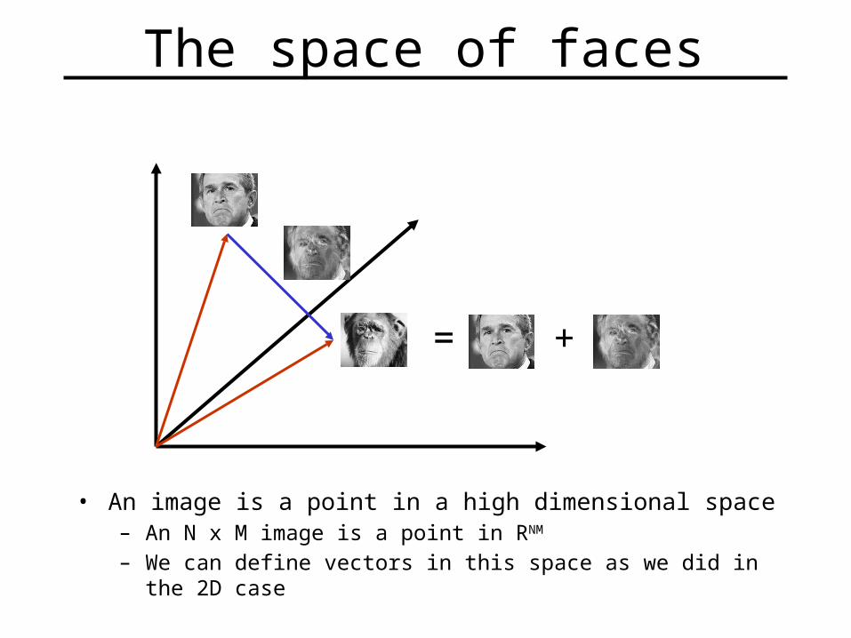
The space of faces

• An image is a point in a high dimensional space– An N x M image is a point in RNM

– We can define vectors in this space as we did in the 2D case

+=

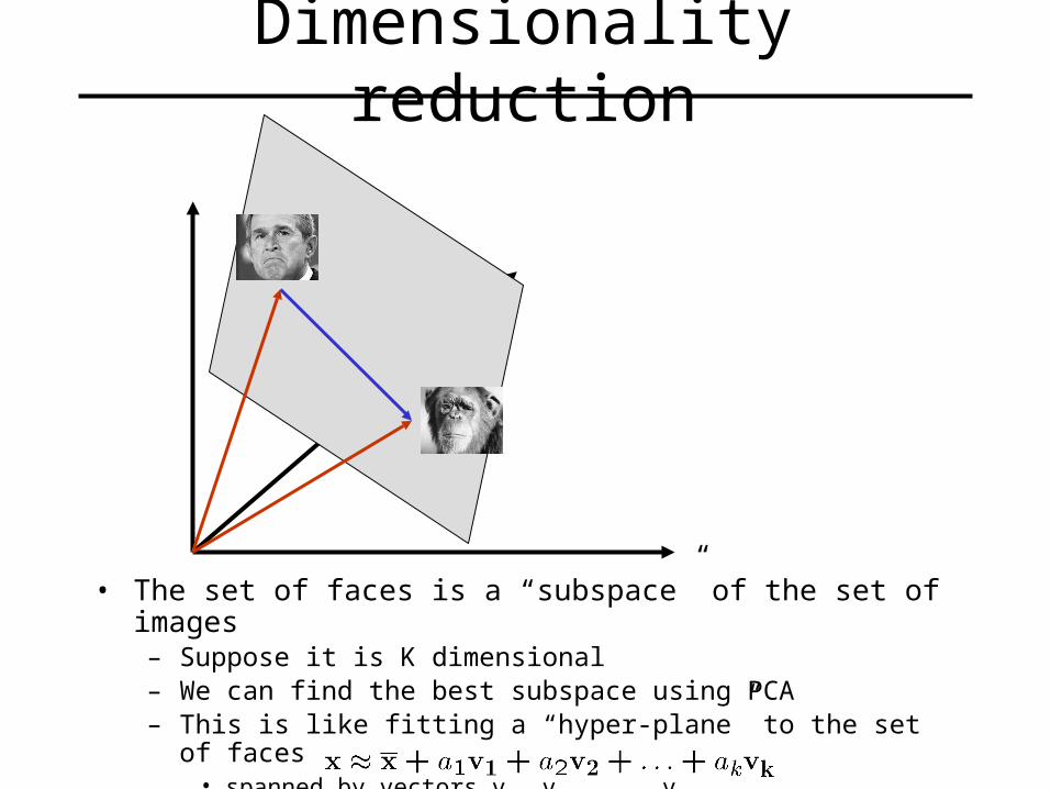
Dimensionality reduction

• The set of faces is a “subspace” of the set of images– Suppose it is K dimensional– We can find the best subspace using PCA– This is like fitting a “hyper-plane” to the set of faces

• spanned by vectors v1, v2, ..., vK

• any face

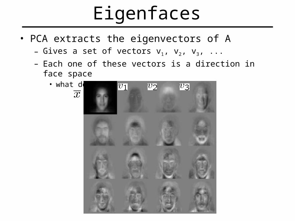
Eigenfaces• PCA extracts the eigenvectors of A

– Gives a set of vectors v1, v2, v3, ...– Each one of these vectors is a direction in face space

• what do these look like?

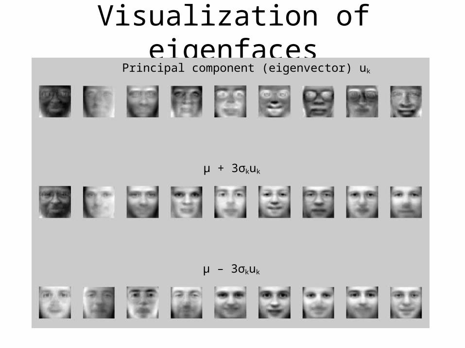
Visualization of eigenfacesPrincipal component (eigenvector) uk

μ + 3σkuk

μ – 3σkuk

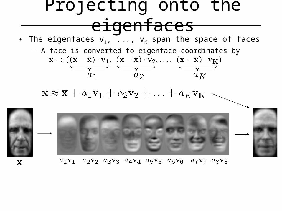
Projecting onto the eigenfaces• The eigenfaces v1, ..., vK span the space of faces

– A face is converted to eigenface coordinates by

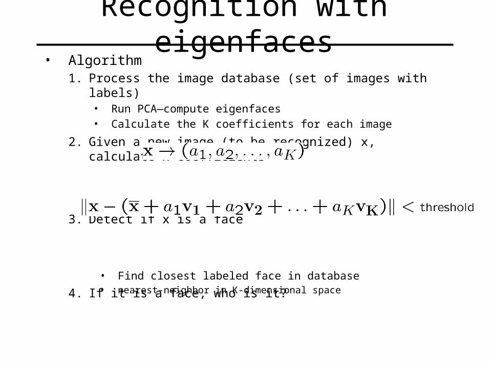
Recognition with eigenfaces• Algorithm

1. Process the image database (set of images with labels)• Run PCA—compute eigenfaces• Calculate the K coefficients for each image

2. Given a new image (to be recognized) x, calculate K coefficients

3. Detect if x is a face

4. If it is a face, who is it?

• Find closest labeled face in database• nearest-neighbor in K-dimensional space

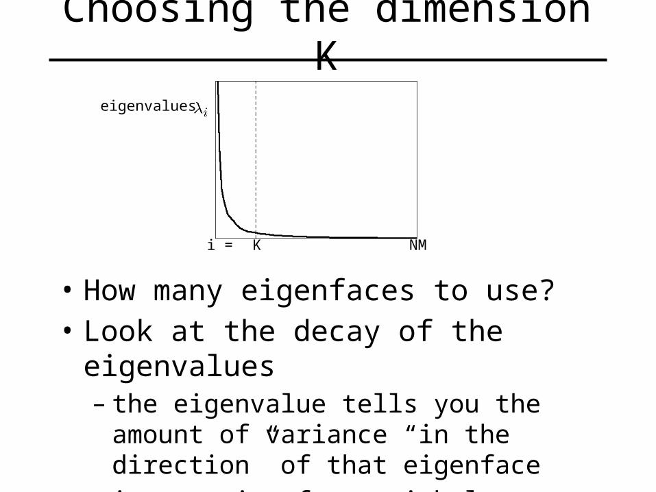
Choosing the dimension K

K NMi =

eigenvalues

• How many eigenfaces to use?• Look at the decay of the eigenvalues

– the eigenvalue tells you the amount of variance “in the direction” of that eigenface

– ignore eigenfaces with low variance

PCA

• General dimensionality reduction technique

• Preserves most of variance with a much more compact representation– Lower storage requirements (eigenvectors + a few

numbers per face)– Faster matching

Enhancing gender

more same original androgynous more opposite

D. Rowland and D. Perrett, “Manipulating Facial Appearance through Shape and Color,” IEEE CG&A,

September 1995 Slide credit: A. Efros

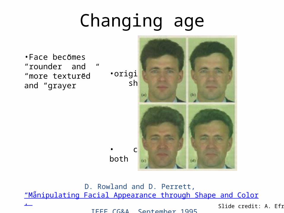
Changing age

•Face becomes “rounder” and “more textured” and “grayer” •original shape

• color both

D. Rowland and D. Perrett, “Manipulating Facial Appearance through Shape and Color,” IEEE CG&A,

September 1995 Slide credit: A. Efros

Which face is more attractive?

http://www.beautycheck.de

Which face is more attractive?leftright

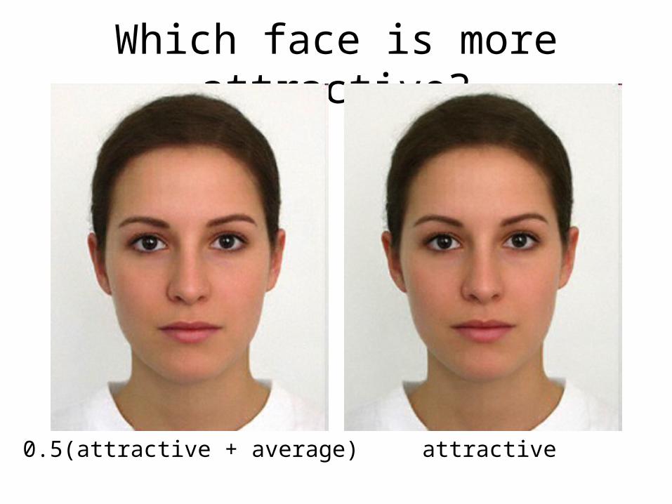
Which face is more attractive?

attractive0.5(attractive + average)

Which face is more attractive?

http://www.beautycheck.de

Which face is more attractive?leftright

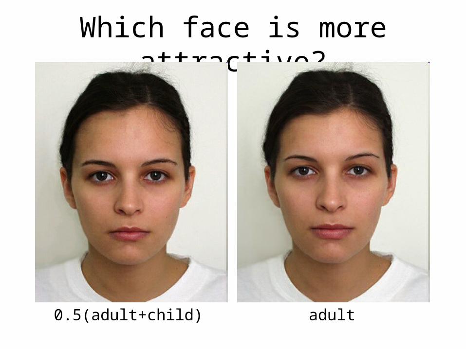
Which face is more attractive?

0.5(adult+child) adult

Limitations• The direction of maximum variance is not

always good for classification

A more discriminative subspace: FLD

• Fisher Linear Discriminants “Fisher Faces”

• PCA preserves maximum variance

• FLD preserves discrimination– Find projection that maximizes scatter between

classes and minimizes scatter within classes

Reference: Eigenfaces vs. Fisherfaces, Belheumer et al., PAMI 1997

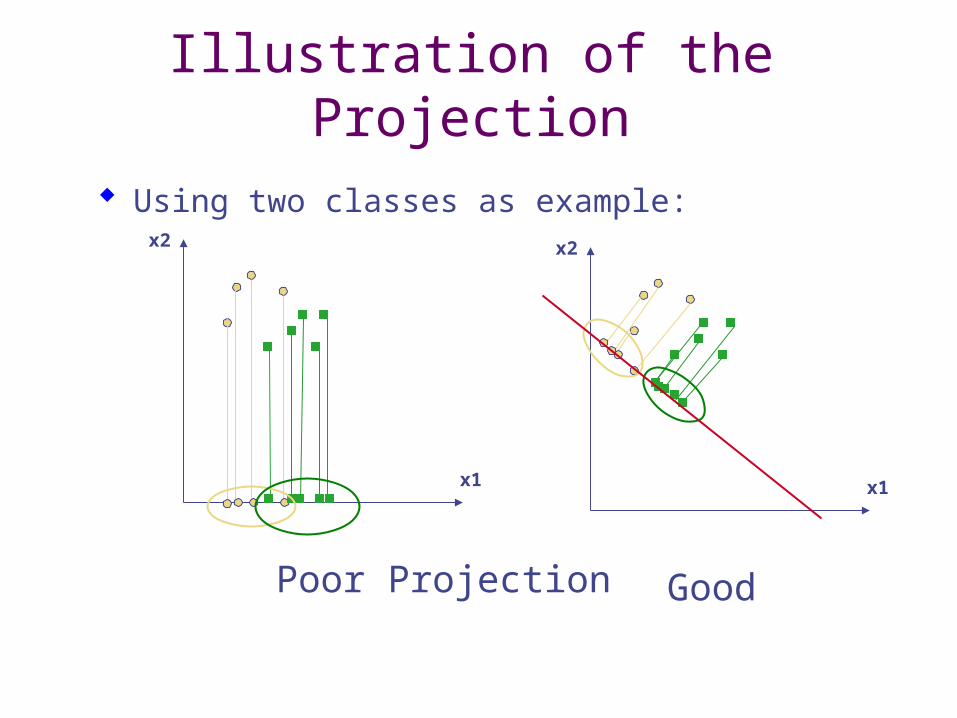
Illustration of the Projection

Poor Projection

x1

x2

x1

x2

Using two classes as example:

Good

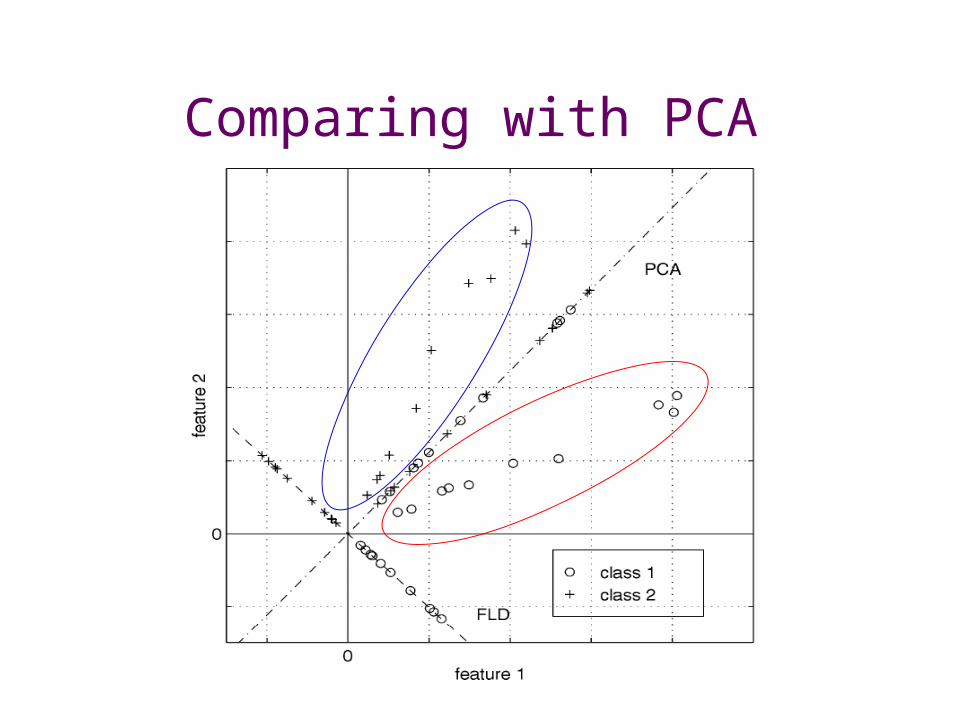
Comparing with PCA

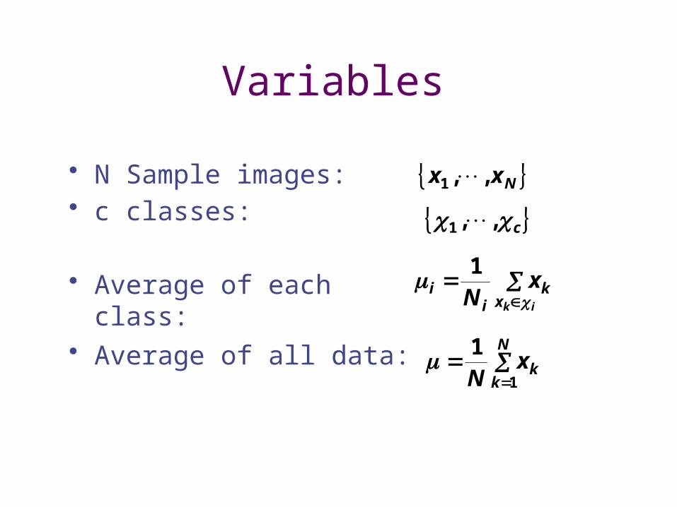
Variables

• N Sample images: • c classes:

• Average of each class:

• Average of all data:

Nxx ,,1

c ,,1

ikx

ki

i xN

1

N

kkxN 1

1

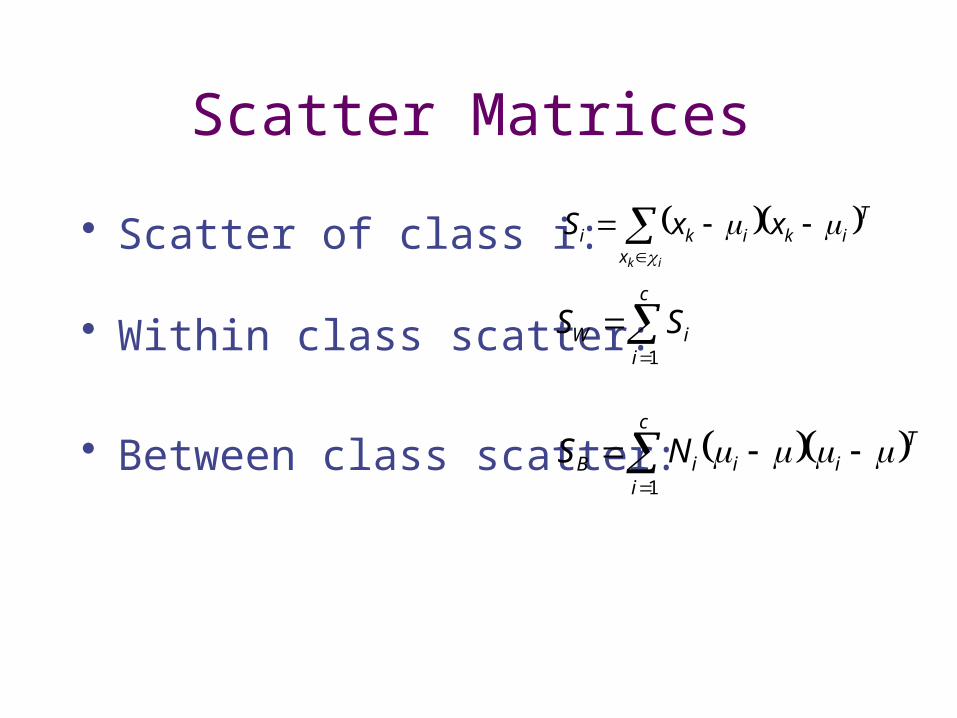
Scatter Matrices

• Scatter of class i: Tikx

iki xxSik

c

iiW SS

1

c

i

TiiiB NS

1

• Within class scatter:

• Between class scatter:

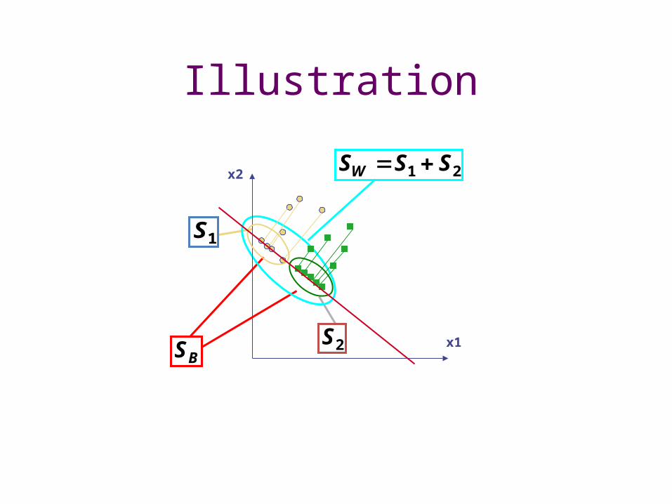
Illustration

2S

1S

BS

21 SSSW

x1

x2Within class scatter

Between class scatter

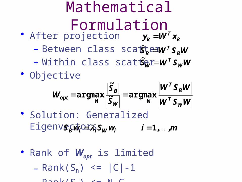
Mathematical Formulation• After projection

– Between class scatter– Within class scatter

• Objective

• Solution: Generalized Eigenvectors

• Rank of Wopt is limited

– Rank(SB) <= |C|-1

– Rank(SW) <= N-C

kT

k xWy

WSWS BT

B ~

WSWS WT

W ~

WSW

WSW

S

SW

WT

BT

W

Bopt

WWmax arg~

~max arg

miwSwS iWiiB ,,1

Illustration

2S

1S

BS

21 SSSW

x1

x2

Recognition with FLD• Use PCA to reduce dimensions to N-C

• Compute within-class and between-class scatter matrices for PCA coefficients

• Solve generalized eigenvector problem

• Project to FLD subspace (c-1 dimensions)

• Classify by nearest neighbor

WSW

WSWW

WT

BT

fldW

max arg miwSwS iWiiB ,,1

Tikx

iki xxSik

c

iiW SS

1

c

i

TiiiB NS

1

xWx Toptˆ

)pca(XWpca

Note: x in step 2 refers to PCA coef; x in step 4 refers to original data

Results: Eigenface vs. Fisherface

• Variation in Facial Expression, Eyewear, and Lighting

• Input:160 images of 16 people• Train:159 images• Test: 1 image

With glasses

Without glasses

3 Lighting conditions

5 expressions

Reference: Eigenfaces vs. Fisherfaces, Belheumer et al., PAMI 1997

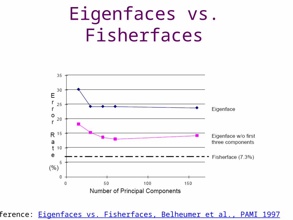
Eigenfaces vs. Fisherfaces

Reference: Eigenfaces vs. Fisherfaces, Belheumer et al., PAMI 1997

Large scale comparison of methods• FRVT 2006 Report

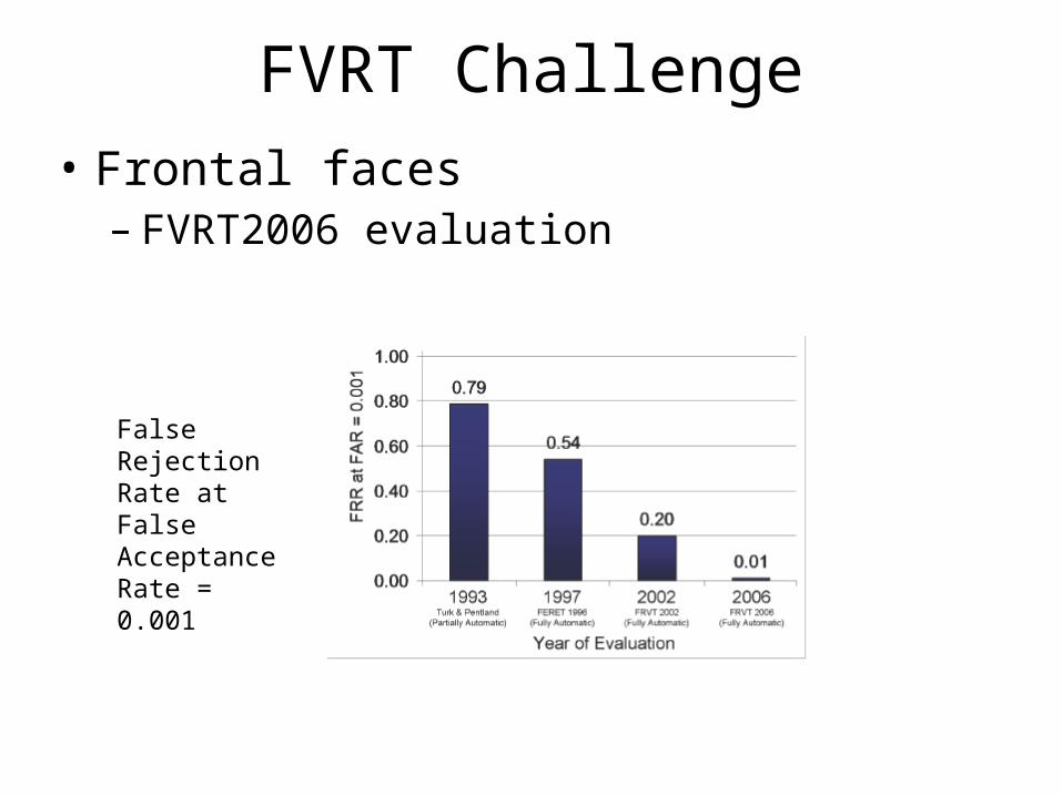
FVRT Challenge• Frontal faces

– FVRT2006 evaluation

False Rejection Rate at False Acceptance Rate = 0.001

FVRT Challenge• Frontal faces

– FVRT2006 evaluation: controlled illumination

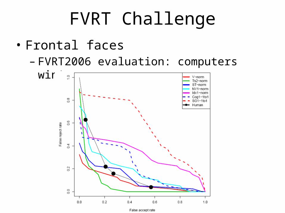
FVRT Challenge• Frontal faces

– FVRT2006 evaluation: computers win!

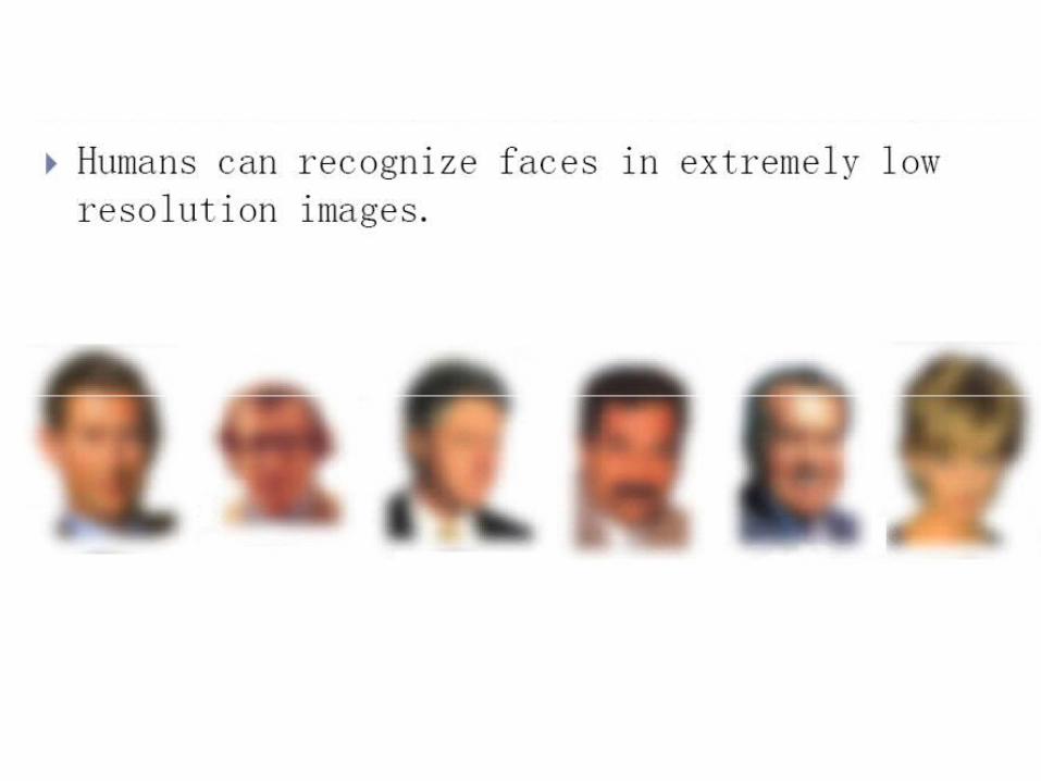
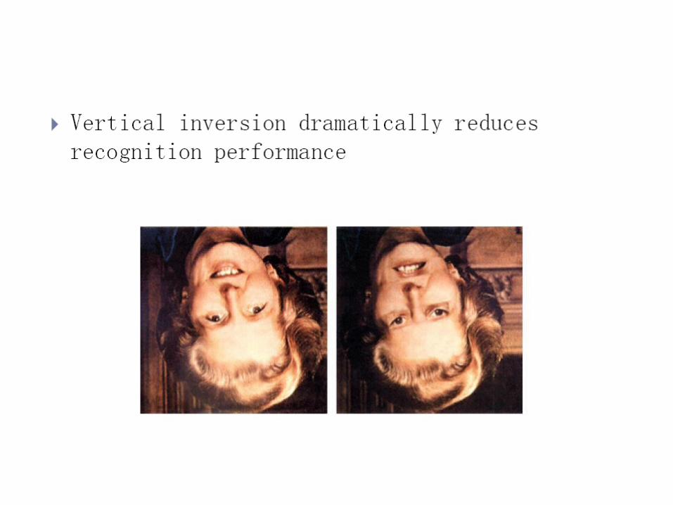
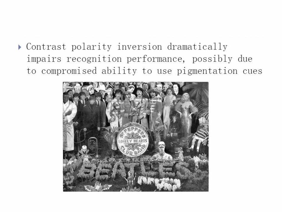
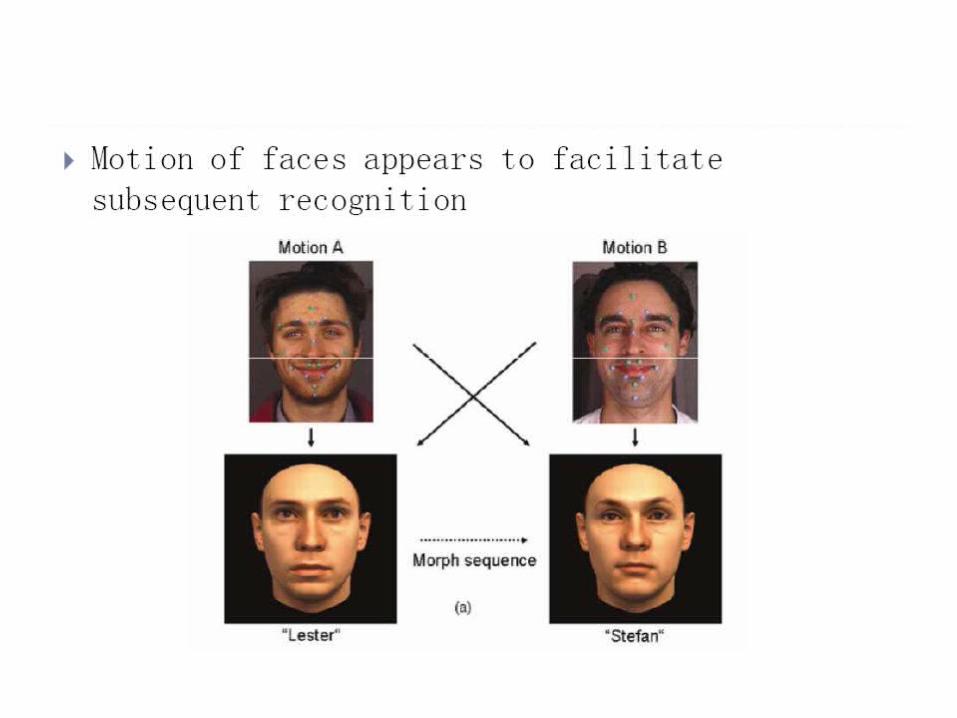
Face recognition by humans

Face recognition by humans: 20 results (2005)

Slides by Jianchao Yang

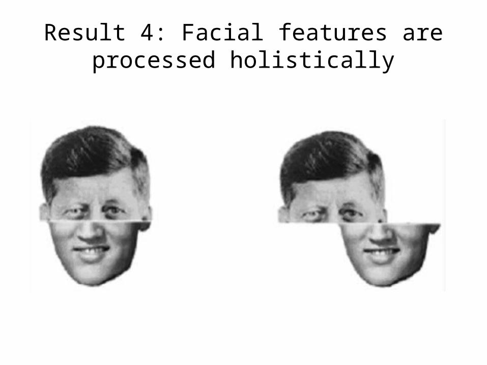
Result 4: Facial features are processed holistically

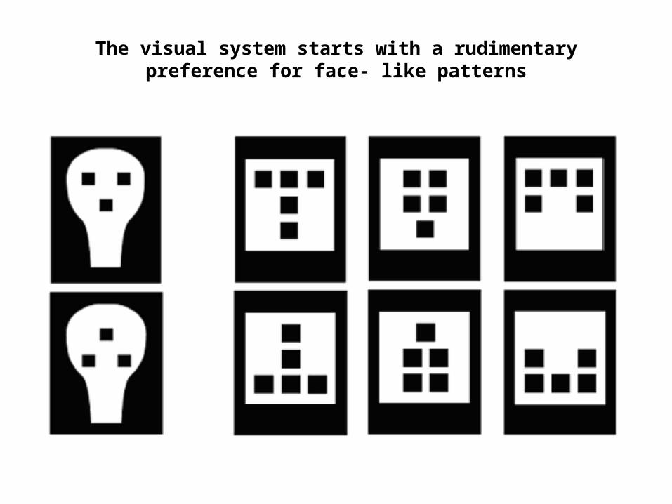
The visual system starts with a rudimentary preference for face- like patterns

Things to remember

• PCA is a generally useful dimensionality reduction technique– But not ideal for discrimination

• FLD better for discrimination, though only ideal under Gaussian data assumptions

• Computer face recognition works very well under controlled environments – still room for improvement in general conditions