face recognition and detection 1 the “margaret thatcher illusion”, by peter thompson...
TRANSCRIPT
Face Recognition and Detection1
Face Recognition and Detection
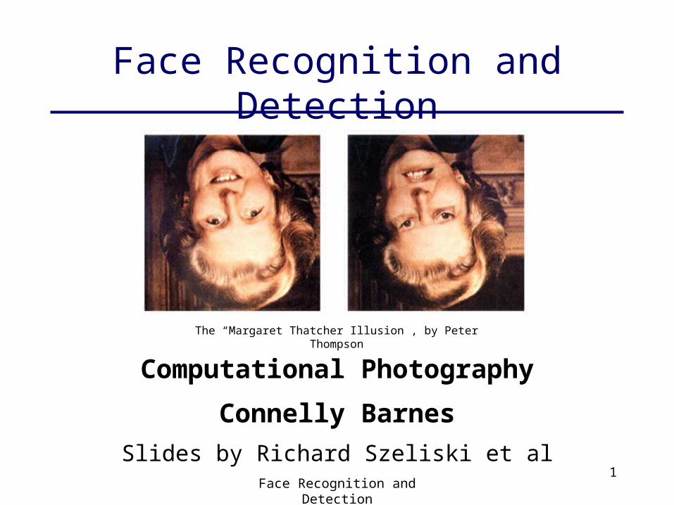
The “Margaret Thatcher Illusion”, by Peter Thompson
Computational Photography
Connelly Barnes
Slides by Richard Szeliski et al
Face Recognition and Detection 2
Recognition problems
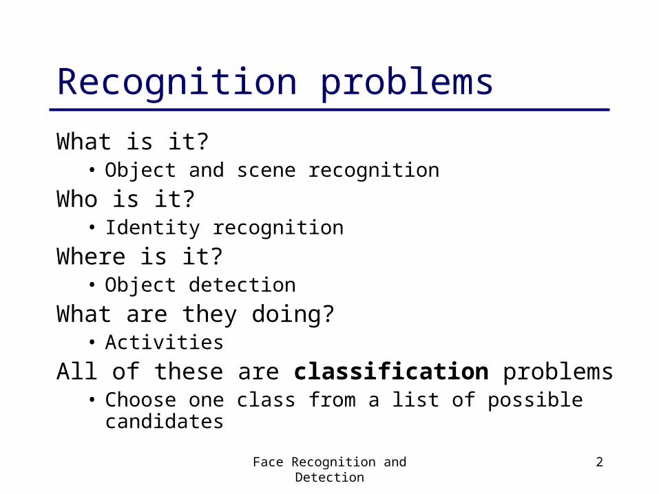
What is it?• Object and scene recognition
Who is it?• Identity recognition
Where is it?• Object detection
What are they doing?• Activities
All of these are classification problems• Choose one class from a list of possible candidates
Face Recognition and Detection 3
What is recognition?
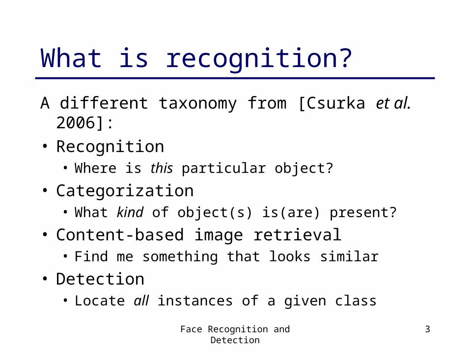
A different taxonomy from [Csurka et al. 2006]:• Recognition
• Where is this particular object?
• Categorization• What kind of object(s) is(are) present?
• Content-based image retrieval• Find me something that looks similar
• Detection• Locate all instances of a given class
Face Recognition and Detection 6
Today’s lecture
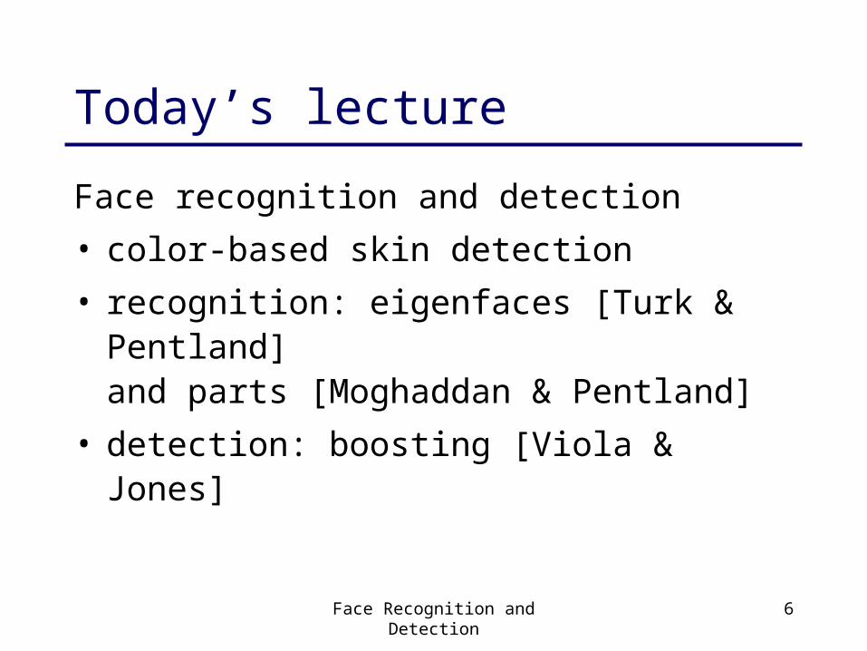
Face recognition and detection
• color-based skin detection
• recognition: eigenfaces [Turk & Pentland]and parts [Moghaddan & Pentland]
• detection: boosting [Viola & Jones]
Face Recognition and Detection 7
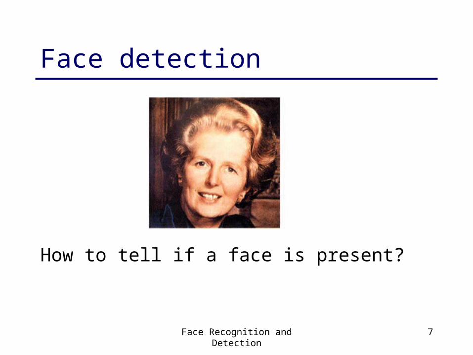
Face detection
How to tell if a face is present?
Face Recognition and Detection 8
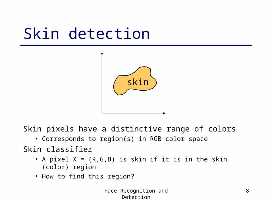
Skin detection
Skin pixels have a distinctive range of colors• Corresponds to region(s) in RGB color space
Skin classifier• A pixel X = (R,G,B) is skin if it is in the skin (color) region• How to find this region?
skin
Face Recognition and Detection 9
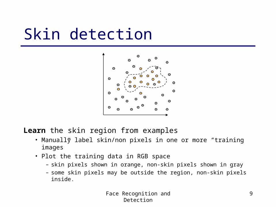
Skin detection
Learn the skin region from examples• Manually label skin/non pixels in one or more “training images”• Plot the training data in RGB space
– skin pixels shown in orange, non-skin pixels shown in gray
– some skin pixels may be outside the region, non-skin pixels inside.
Face Recognition and Detection 10
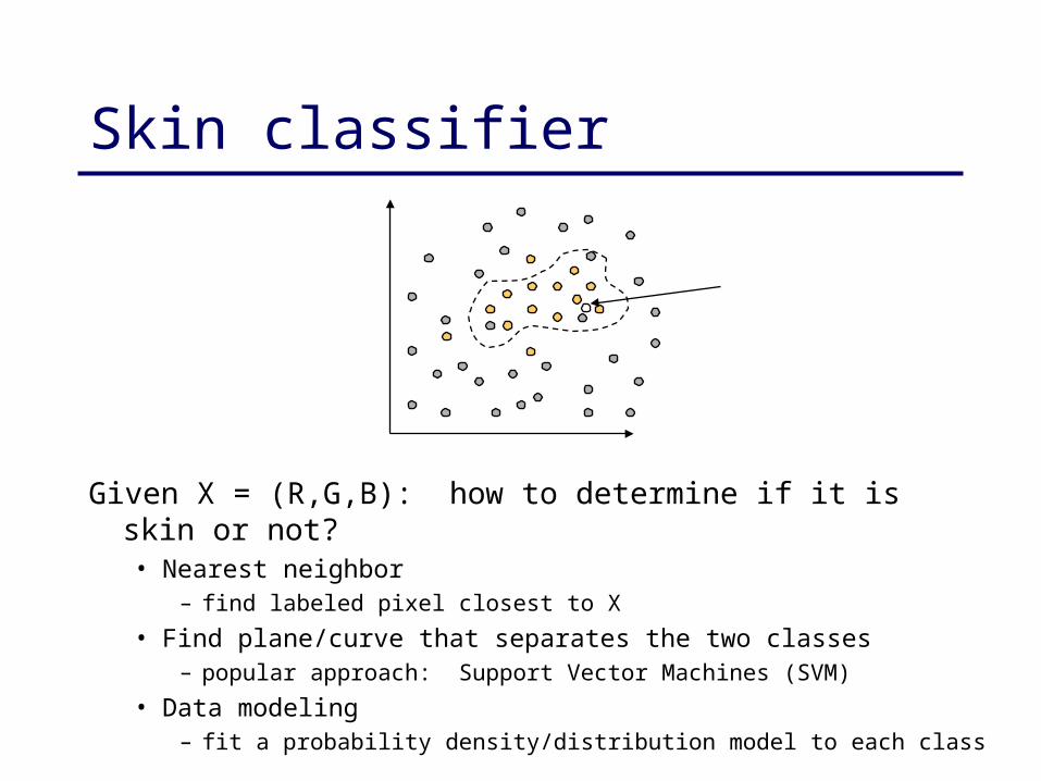
Skin classifier
Given X = (R,G,B): how to determine if it is skin or not?• Nearest neighbor
– find labeled pixel closest to X
• Find plane/curve that separates the two classes– popular approach: Support Vector Machines (SVM)
• Data modeling– fit a probability density/distribution model to each class
Face Recognition and Detection 11
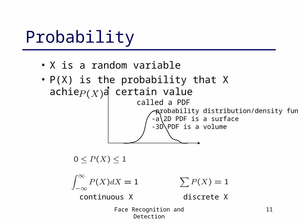
Probability
• X is a random variable• P(X) is the probability that X achieves a certain
value
continuous X discrete X
called a PDF-probability distribution/density function-a 2D PDF is a surface-3D PDF is a volume
Face Recognition and Detection 12
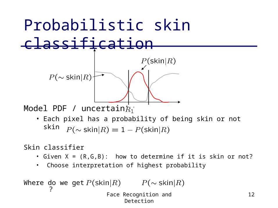
Probabilistic skin classification
Model PDF / uncertainty• Each pixel has a probability of being skin or not skin
Skin classifier• Given X = (R,G,B): how to determine if it is skin or not?
• Choose interpretation of highest probability
Where do we get and ?
Face Recognition and Detection 13
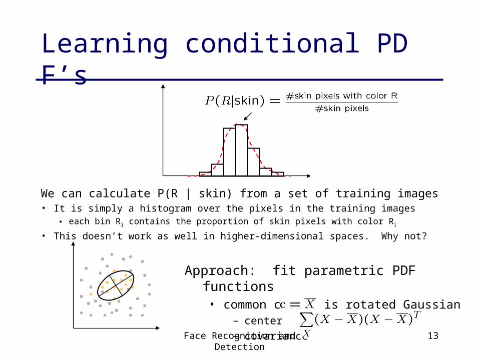
Learning conditional PDF’s
We can calculate P(R | skin) from a set of training images• It is simply a histogram over the pixels in the training images
• each bin Ri contains the proportion of skin pixels with color Ri
• This doesn’t work as well in higher-dimensional spaces. Why not?Approach: fit parametric PDF functions
• common choice is rotated Gaussian – center – covariance
Face Recognition and Detection 14
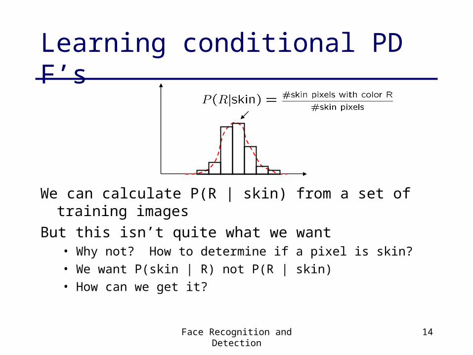
Learning conditional PDF’s
We can calculate P(R | skin) from a set of training images
But this isn’t quite what we want• Why not? How to determine if a pixel is skin?• We want P(skin | R) not P(R | skin)• How can we get it?
Face Recognition and Detection 15
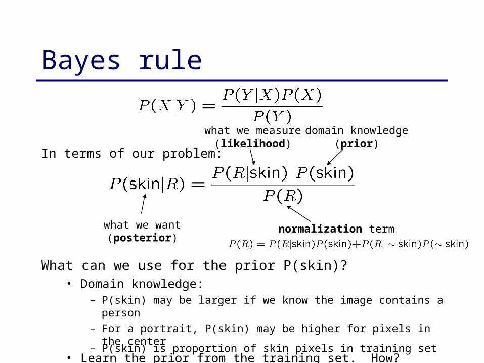
Bayes rule
In terms of our problem:
what we measure(likelihood)
domain knowledge(prior)
what we want(posterior)
normalization term
What can we use for the prior P(skin)?• Domain knowledge:
– P(skin) may be larger if we know the image contains a person– For a portrait, P(skin) may be higher for pixels in the center
• Learn the prior from the training set. How?– P(skin) is proportion of skin pixels in training set
Face Recognition and Detection 16
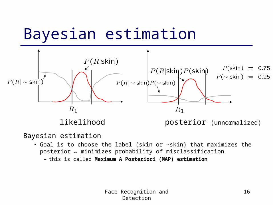
Bayesian estimation
Bayesian estimation• Goal is to choose the label (skin or ~skin) that maximizes the posterior ↔
minimizes probability of misclassification– this is called Maximum A Posteriori (MAP) estimation
likelihood posterior (unnormalized)
Face Recognition and Detection 17
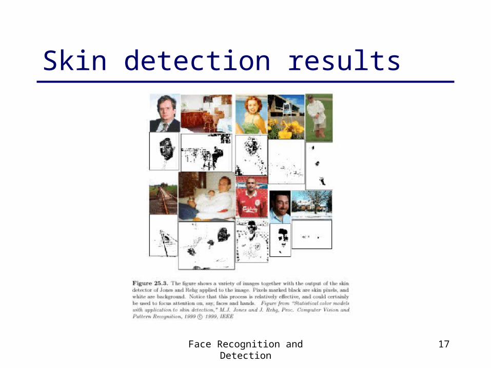
Skin detection results
Face Recognition and Detection 18
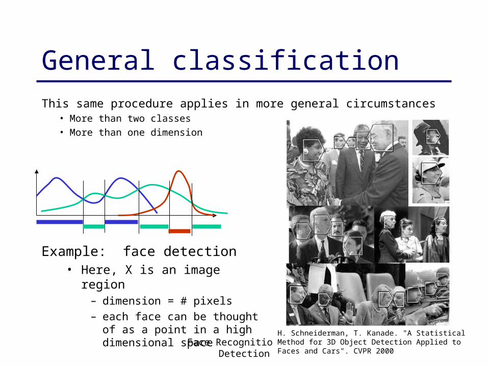
This same procedure applies in more general circumstances• More than two classes• More than one dimension
General classification
Example: face detection• Here, X is an image region
– dimension = # pixels – each face can be thought of as a
point in a high dimensional space
H. Schneiderman, T. Kanade. "A Statistical Method for 3D Object Detection Applied to Faces and Cars". CVPR 2000
Face Recognition and Detection 19
Today’s lecture
Face recognition and detection• color-based skin detection• recognition: eigenfaces [Turk & Pentland]
and parts [Moghaddan & Pentland]• detection: boosting [Viola & Jones]
Eigenfaces for recognition
Matthew Turk and Alex Pentland
J. Cognitive Neuroscience
1991
Face Recognition and Detection 21
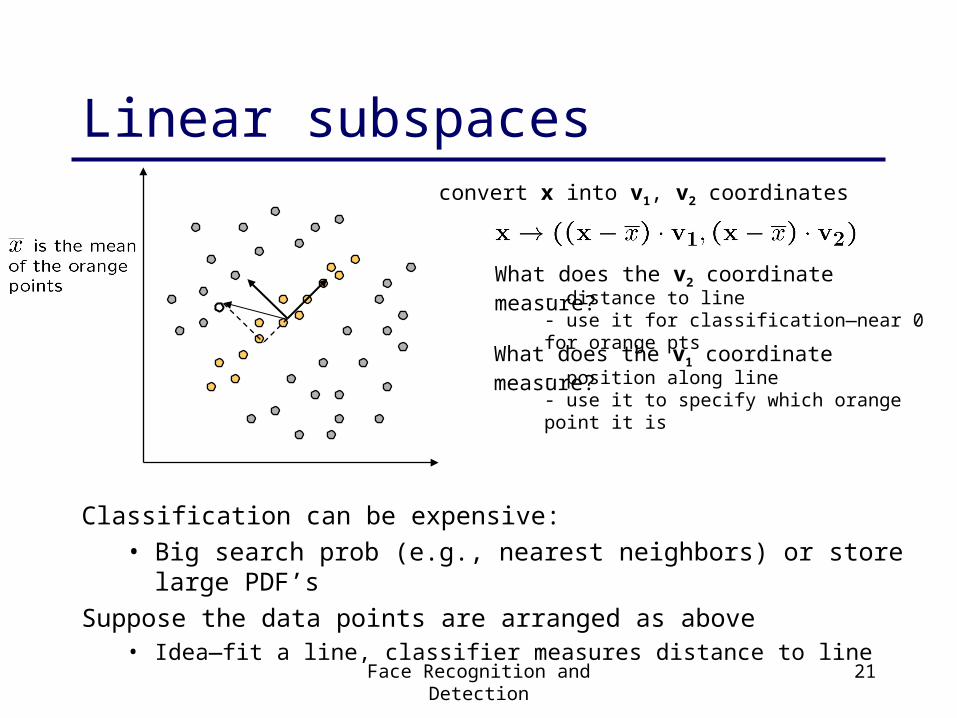
Linear subspaces
Classification can be expensive:• Big search prob (e.g., nearest neighbors) or store large PDF’s
Suppose the data points are arranged as above• Idea—fit a line, classifier measures distance to line
convert x into v1, v2 coordinates
What does the v2 coordinate measure?
What does the v1 coordinate measure?
- distance to line- use it for classification—near 0 for orange pts
- position along line- use it to specify which orange point it is
Face Recognition and Detection 22
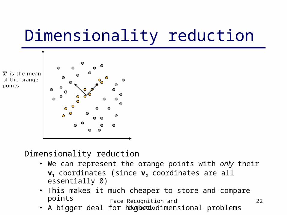
Dimensionality reduction
Dimensionality reduction• We can represent the orange points with only their v1 coordinates
(since v2 coordinates are all essentially 0)• This makes it much cheaper to store and compare points• A bigger deal for higher dimensional problems
Face Recognition and Detection 23
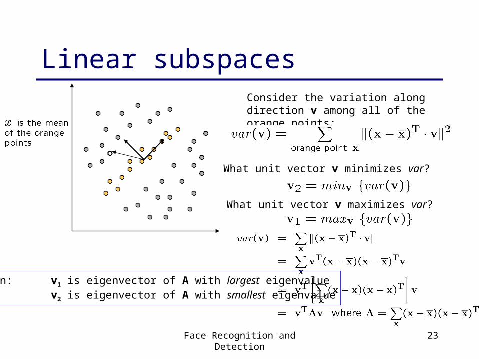
Linear subspacesConsider the variation along direction v among all of the orange points:
What unit vector v minimizes var?
What unit vector v maximizes var?
Solution: v1 is eigenvector of A with largest eigenvalue v2 is eigenvector of A with smallest eigenvalue
Face Recognition and Detection 24
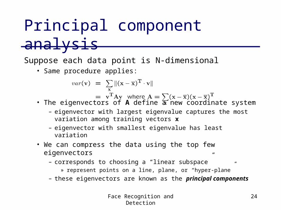
Principal component analysis
Suppose each data point is N-dimensional• Same procedure applies:
• The eigenvectors of A define a new coordinate system– eigenvector with largest eigenvalue captures the most variation
among training vectors x
– eigenvector with smallest eigenvalue has least variation
• We can compress the data using the top few eigenvectors– corresponds to choosing a “linear subspace”
» represent points on a line, plane, or “hyper-plane”
– these eigenvectors are known as the principal components
Face Recognition and Detection 25
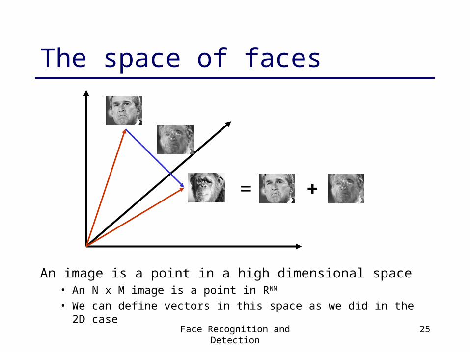
The space of faces
An image is a point in a high dimensional space• An N x M image is a point in RNM
• We can define vectors in this space as we did in the 2D case
+=
Face Recognition and Detection 26
Dimensionality reduction
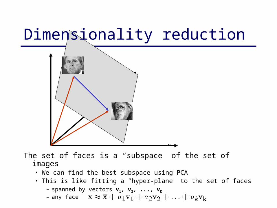
The set of faces is a “subspace” of the set of images• We can find the best subspace using PCA• This is like fitting a “hyper-plane” to the set of faces
– spanned by vectors v1, v2, ..., vK
– any face
Face Recognition and Detection 27
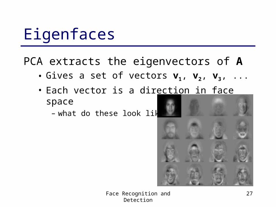
Eigenfaces
PCA extracts the eigenvectors of A• Gives a set of vectors v1, v2, v3, ...
• Each vector is a direction in face space– what do these look like?
Face Recognition and Detection 28
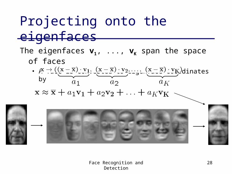
Projecting onto the eigenfaces
The eigenfaces v1, ..., vK span the space of faces• A face is converted to eigenface coordinates by
Face Recognition and Detection 29
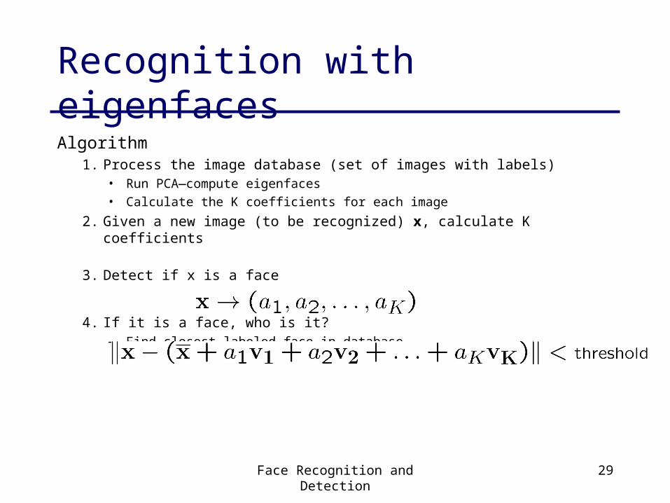
Recognition with eigenfaces
Algorithm1. Process the image database (set of images with labels)
• Run PCA—compute eigenfaces
• Calculate the K coefficients for each image
2. Given a new image (to be recognized) x, calculate K coefficients
3. Detect if x is a face
4. If it is a face, who is it?– Find closest labeled face in database
» nearest-neighbor in K-dimensional space
Face Recognition and Detection 30
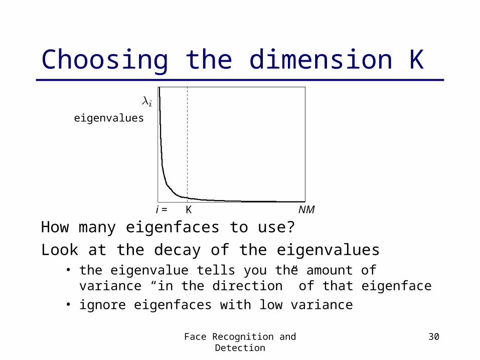
Choosing the dimension K
K NMi =
eigenvalues
How many eigenfaces to use?
Look at the decay of the eigenvalues• the eigenvalue tells you the amount of variance “in the
direction” of that eigenface• ignore eigenfaces with low variance

View-Based and Modular Eigenspaces for Face Recognition
Alex Pentland, Baback Moghaddam and Thad Starner
CVPR’94
Face Recognition and Detection 32
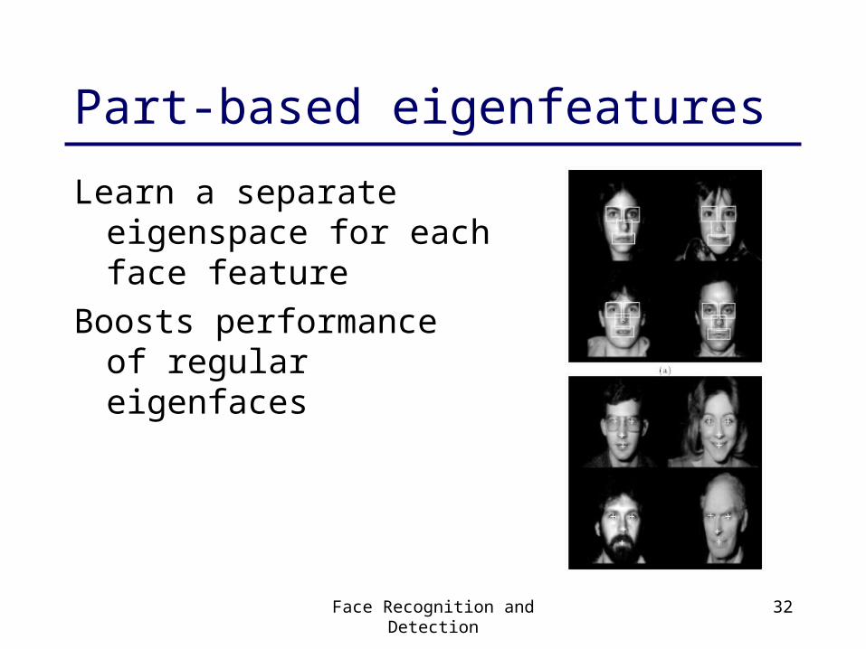
Part-based eigenfeatures
Learn a separateeigenspace for eachface feature
Boosts performanceof regulareigenfaces
Bayesian Face Recognition
Baback Moghaddam, Tony Jebaraand Alex Pentland
Pattern Recognition
33(11), 1771-1782, November 2000(slides from Bill Freeman, MIT 6.869, April 2005)
Face Recognition and Detection 34
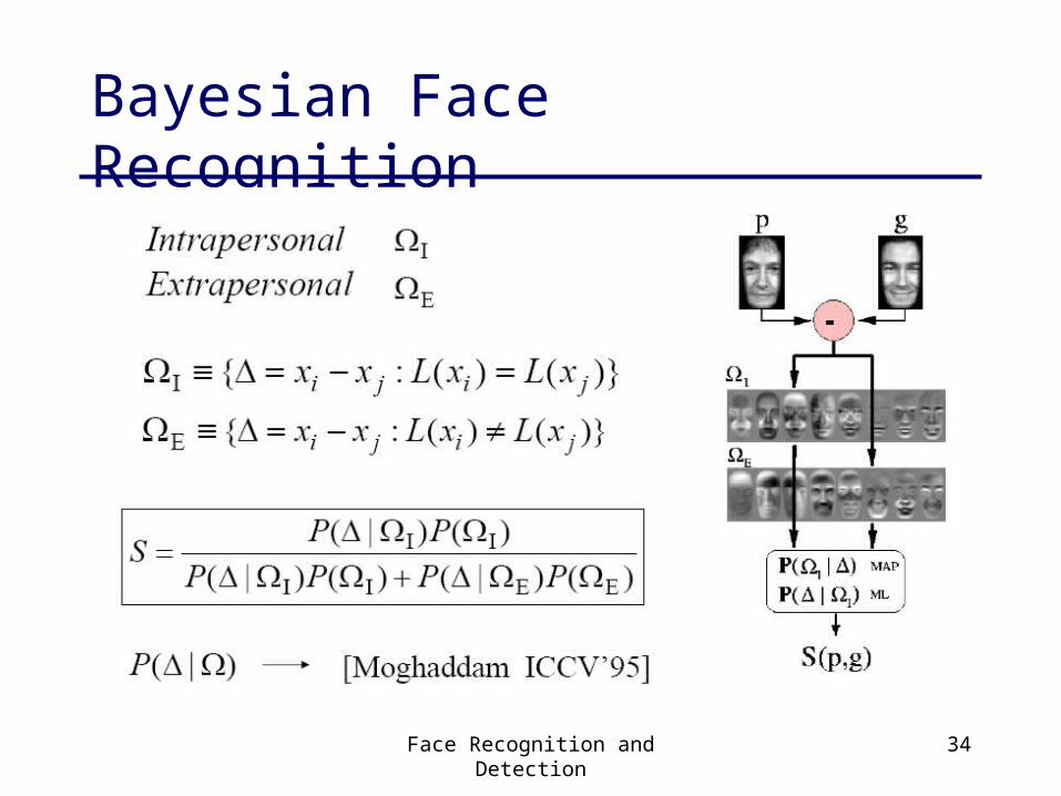
Bayesian Face Recognition
Face Recognition and Detection 35
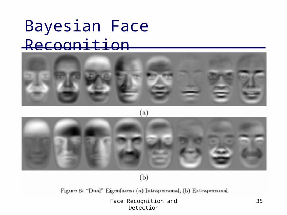
Bayesian Face Recognition
Face Recognition and Detection 36
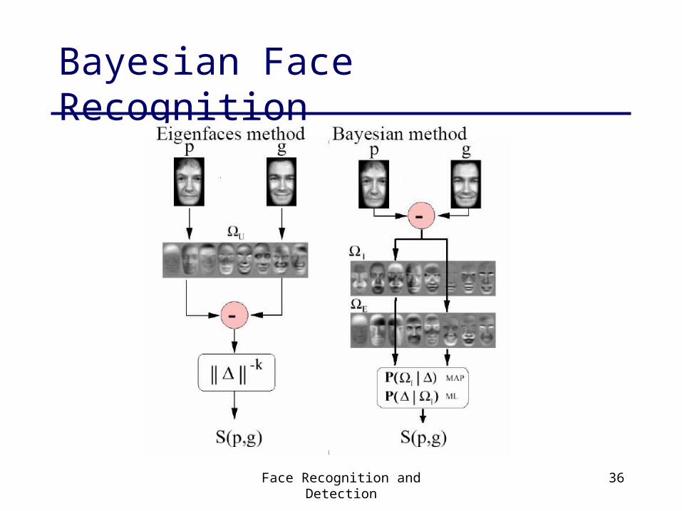
Bayesian Face Recognition
Morphable Face Models
Rowland and Perrett ’95
Lanitis, Cootes, and Taylor ’95, ’97
Blanz and Vetter ’99
Matthews and Baker ’04, ‘07
Face Recognition and Detection 38
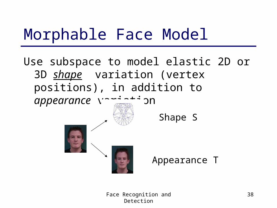
Morphable Face Model
Use subspace to model elastic 2D or 3D shape variation (vertex positions), in addition to appearance variation
Shape S
Appearance T
Face Recognition and Detection 39
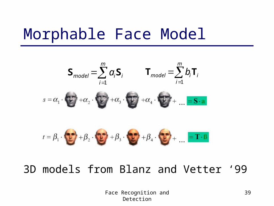
Morphable Face Model
3D models from Blanz and Vetter ‘99
m
iiimodel a
1
SS
m
iiimodel b
1
TT
Face Recognition and Detection 40
Face Recognition Resources
Face Recognition Home Page:• http://www.cs.rug.nl/~peterkr/FACE/face.html
PAMI Special Issue on Face & Gesture (July ‘97)
FERET• http://www.dodcounterdrug.com/facialrecognition/Feret/feret.htm
Face-Recognition Vendor Test (FRVT 2000)• http://www.dodcounterdrug.com/facialrecognition/FRVT2000/frvt2000.htm
Biometrics Consortium• http://www.biometrics.org
Face Recognition and Detection 41
Today’s lecture
Face recognition and detection• color-based skin detection• recognition: eigenfaces [Turk & Pentland]
and parts [Moghaddan & Pentland]• detection: boosting [Viola & Jones]
Robust real-time face detection
Paul A. Viola and Michael J. Jones
Intl. J. Computer Vision
57(2), 137–154, 2004
(originally in CVPR’2001)(slides adapted from Bill Freeman, MIT 6.869, April 2005)
Face Recognition and Detection 43
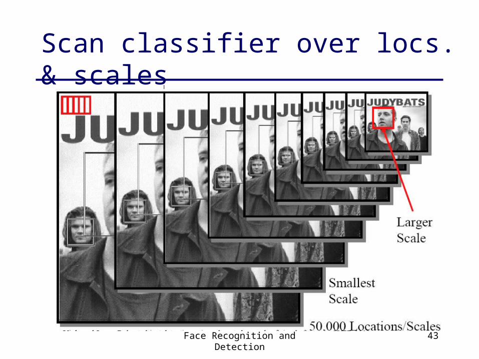
Scan classifier over locs. & scales
Face Recognition and Detection 44
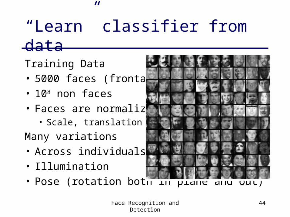
“Learn” classifier from data
Training Data• 5000 faces (frontal)• 108 non faces• Faces are normalized
• Scale, translation
Many variations• Across individuals• Illumination• Pose (rotation both in plane and out)
Face Recognition and Detection 45
Characteristics of algorithm
• Feature set (…is huge about 16M features)• Efficient feature selection using AdaBoost• Image representation: Integral Image (also
known as summed area tables)• Cascaded Classifier for rapid detection
Fastest known face detector for gray scale images
Face Recognition and Detection 46
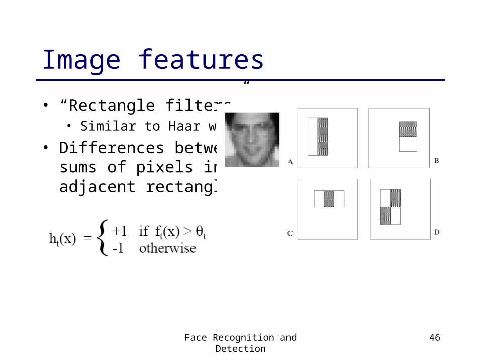
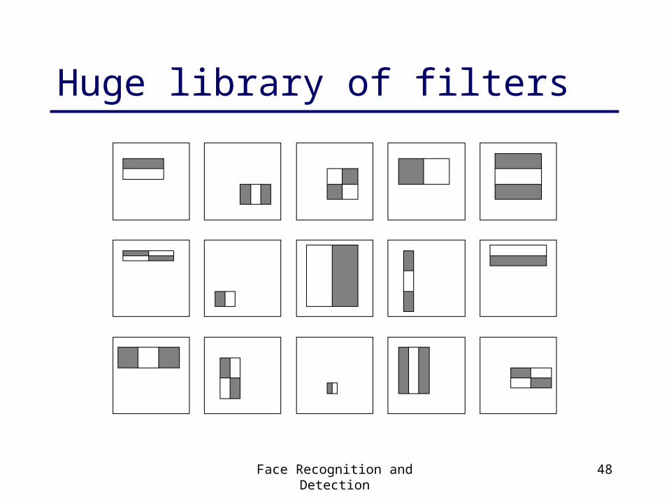
Image features
• “Rectangle filters”• Similar to Haar wavelets
• Differences between sums of pixels inadjacent rectangles
Face Recognition and Detection 47
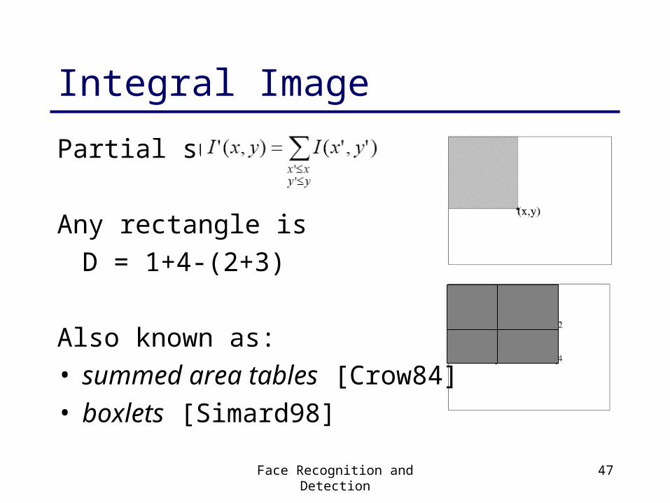
Partial sum
Any rectangle is
D = 1+4-(2+3)
Also known as:• summed area tables [Crow84]• boxlets [Simard98]
Integral Image
Face Recognition and Detection 48
Huge library of filters
Face Recognition and Detection 49
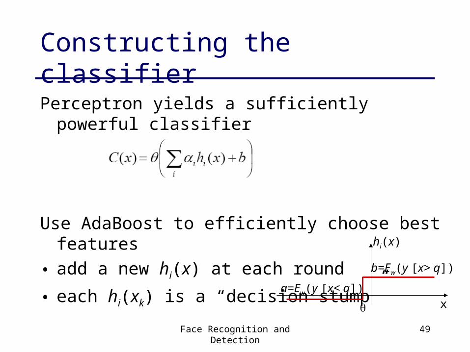
Constructing the classifier
Perceptron yields a sufficiently powerful classifier
Use AdaBoost to efficiently choose best features
• add a new hi(x) at each round
• each hi(xk) is a “decision stump” b=Ew(y [x> q])
a=Ew(y [x< q])x
hi(x)
Face Recognition and Detection 50
Constructing the classifier
For each round of boosting:• Evaluate each rectangle filter on each example• Sort examples by filter values• Select best threshold for each filter (min error)
• Use sorting to quickly scan for optimal threshold
• Select best filter/threshold combination• Weight is a simple function of error rate• Reweight examples
• (There are many tricks to make this more efficient.)
Face Recognition and Detection 52
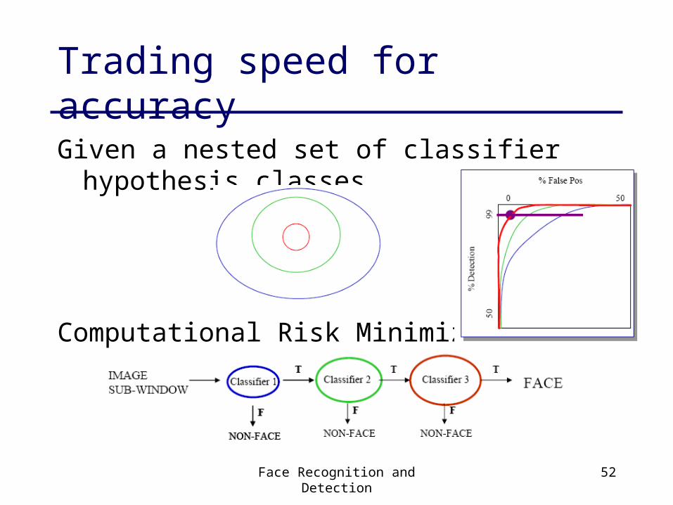
Trading speed for accuracy
Given a nested set of classifier hypothesis classes
Computational Risk Minimization
Face Recognition and Detection 53
Speed of face detector (2001)
Speed is proportional to the average number of features computed per sub-window.
On the MIT+CMU test set, an average of 9 features (/ 6061) are computed per sub-window.
On a 700 Mhz Pentium III, a 384x288 pixel image takes about 0.067 seconds to process (15 fps).
Roughly 15 times faster than Rowley-Baluja-Kanade and 600 times faster than Schneiderman-Kanade.
Face Recognition and Detection 54
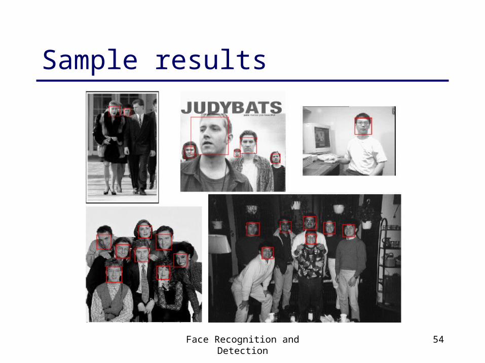
Sample results
Face Recognition and Detection 55
Summary (Viola-Jones)
• Fastest known face detector for gray images• Three contributions with broad applicability:
Cascaded classifier yields rapid classification
AdaBoost as an extremely efficient feature selector
Rectangle Features + Integral Image can be used for rapid image analysis
Face Recognition and Detection 56
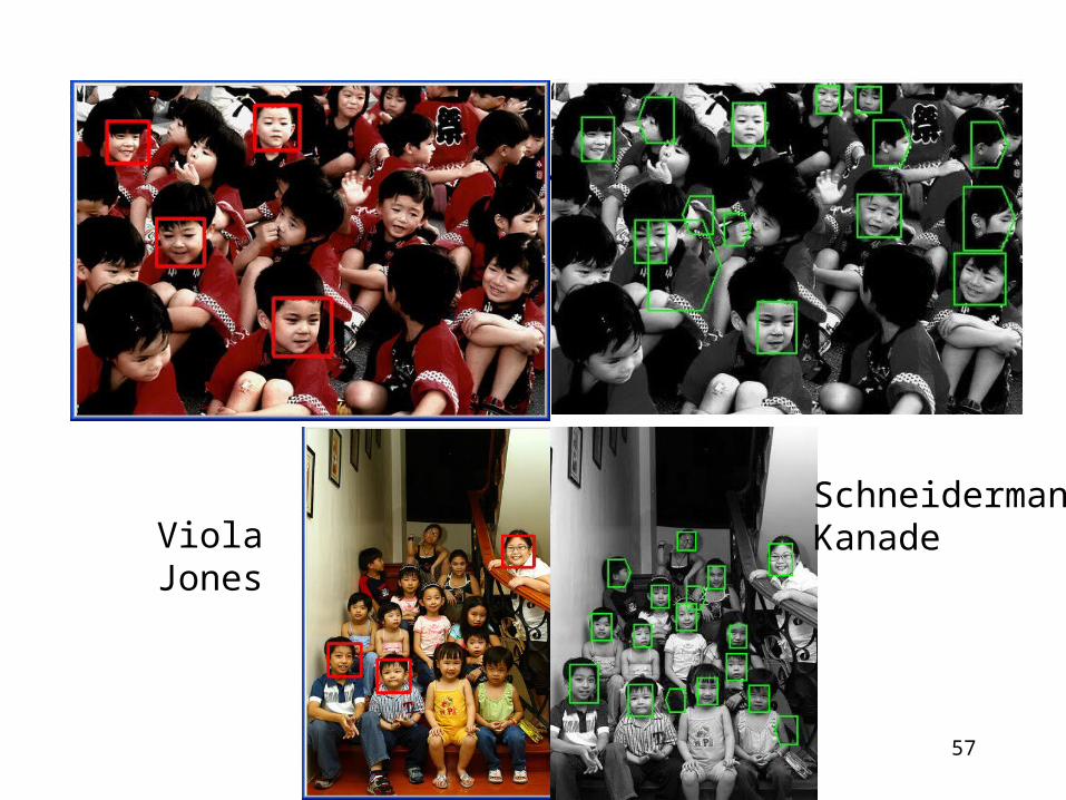
Face detector comparison
Informal study by Andrew Gallagher, CMU,for CMU 16-721 Learning-Based Methods in Vision, Spring 2007 • The Viola Jones algorithm OpenCV
implementation was used. (<2 sec per image). • For Schneiderman and Kanade, Object Detection
Using the Statistics of Parts [IJCV’04], the www.pittpatt.com demo was used. (~10-15 seconds per image, including web transmission).
Face Recognition and Detection 57
SchneidermanKanadeViola
Jones

Face Recognition and Detection 58
Today’s lecture
Face recognition and detection
• color-based skin detection
• recognition: eigenfaces [Turk & Pentland]and parts [Moghaddan & Pentland]
• detection: boosting [Viola & Jones]
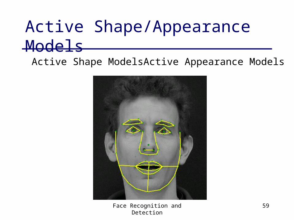
Active Shape/Appearance Models
Face Recognition and Detection 59
Active Shape Models Active Appearance Models

Questions?