face recognition based on videos by using convex hulls

HAL Id: hal-03044541https://hal.archives-ouvertes.fr/hal-03044541

Submitted on 7 Dec 2020

HAL is a multi-disciplinary open accessarchive for the deposit and dissemination of sci-entific research documents, whether they are pub-lished or not. The documents may come fromteaching and research institutions in France orabroad, or from public or private research centers.

L’archive ouverte pluridisciplinaire HAL, estdestinée au dépôt et à la diffusion de documentsscientifiques de niveau recherche, publiés ou non,émanant des établissements d’enseignement et derecherche français ou étrangers, des laboratoirespublics ou privés.

Face Recognition Based on Videos by Using ConvexHulls

Hakan Cevikalp, Hasan Serhan Yavuz, Bill Triggs

To cite this version:Hakan Cevikalp, Hasan Serhan Yavuz, Bill Triggs. Face Recognition Based on Videos by Using ConvexHulls. IEEE Transactions on Circuits and Systems for Video Technology, Institute of Electrical andElectronics Engineers, 2020, 30 (12), pp.4481-4495. �10.1109/TCSVT.2019.2926165�. �hal-03044541�

https://hal.archives-ouvertes.fr/hal-03044541

https://hal.archives-ouvertes.fr

1051-8215 (c) 2019 IEEE. Personal use is permitted, but republication/redistribution requires IEEE permission. See http://www.ieee.org/publications_standards/publications/rights/index.html for more information.

This article has been accepted for publication in a future issue of this journal, but has not been fully edited. Content may change prior to final publication. Citation information: DOI 10.1109/TCSVT.2019.2926165, IEEE

Transactions on Circuits and Systems for Video Technology

JOURNAL OF IEEE TRANSACTIONS ON CIRCUITS AND SYSTEMS FOR VIDEO TECHNOLOGY, VOL. X, NO. X, JULY 2017 1

Face Recognition Based on Videos by UsingConvex Hulls

Hakan Cevikalp, Member, IEEE, Hasan Serhan Yavuz, Member, IEEE, and Bill Triggs, Member, IEEE

Abstract—A wide range of face appearance variations can be modeled by using set based recognition approaches effectively, but

computational complexity of current methods is highly dependent on the set and class sizes. This paper introduces new video based

classification methods designed for reducing the required disk space of data samples and speed up the testing process in large-scale

face recognition systems. In the proposed method, image sets collected from videos are approximated with kernelized convex hulls

and it was shown that it is sufficient to use only the samples that participate in shaping the image set boundaries in this setting. The

kernelized Support Vector Data Description (SVDD) is used to extract those important samples that form the image set boundaries.

Moreover, we show that these kernelized hypersphere models can also be used to approximate image sets for classification purposes.

Then, we propose a binary hierarchical decision tree approach to improve the speed of the classification system even more. Lastly, we

introduce a new video database that includes 285 people with 8 videos of each person since the most popular video data sets used for

set based recognition methods include either a few people, or small number of videos per person. The experimental results on varying

sized databases show that the proposed methods greatly improve the testing times of the classification system (we obtained

speed-ups to a factor of 20) without a significant drop in accuracies.

Index Terms—Face Recognition, Image Set Classification, Affine Hulls, Convex Hulls, Support Vector Data Description, Binary

Hierarchical Tree.

✦

1 INTRODUCTION

F ACE recognition systems find their applications in various

fields. Rather than typically being used in security systems,

wide use of video or cell phone cameras have led to identifying

people in daily life such as tagging a friend on social media or

searching for some people among numerous videos etc.. In gen-

eral, face recognition process can involve 1) single image based

or 2) video (collection of a set of images) based classification

tasks. For set based face recognition, both gallery and query

sets are given in terms of sets of images rather than a single

image. Images can be collected from video frames as well as

from multiple unordered observations. The classification system

must return the individual whose gallery set is the most similar

to the given query set. Set based methods usually perform better

than the methods using single images since image sets include

variability of the individual’s appearance. These methods are also

more practical owing to the fact that they usually do not require

any cooperation from persons. However, despite these advantages,

traditional classifiers such as Support Vector Machines (SVMs),

classification trees, k-nearest neighbor (k-NN) etc. cannot be used

directly, which can be considered as a major limitation of the set

based methods.

Based on the set model representation types, existing set based

methods can be roughly divided into two categories, parametric

and non-parametric methods. Probability distributions such as

Gaussians or mixture of them were used to model image sets in

parametric methods such as [1,2], and the similarity (or dissimilar-

ity) is measured by using the distribution divergences. However,

these methods do not perform well in cases where the test sets

have only weak statistical relationships to the training ones as

• H. Cevikalp and H. S. Yavuz are with the Department of Electrical and

Electronics Engineering, Eskisehir Osmangazi University, 26480, Turkey.

B. Triggs is with Laboratoire Jean Kuntzmann, Grenoble, France.

E-mail: see http://mlcv.ogu.edu.tr/contacts.html

noted in [3,4]. Nonparametric methods, on the other hand, use

different models (e.g., linear or affine subspaces or some different

combinations of these subspaces) to approximate image sets, and

different metrics have been proposed for set-to-set distances based

on the type of utilized models.

As a pioneering work for nonparametric models, Yamaguchi et

al. [5] used linear subspaces to approximate image sets, and canon-

ical angles between subspaces are used to measure the distance

between them. A basic limitation of linear subspace methods is

that the linear subspace angles do not provide strong information

about the locations of the samples (affine subspaces can better

approximate class regions compared to the linear ones). Another

way of dealing with image set based classification is to consider

each sample as a point in a Grassmannian manifold. Hamm

and Lee [6] used Grassmannian discriminant analysis on fixed

dimensional linear subspaces. Wang and Shi [7] proposed kernel

Grassmannian distances to compare image sets. Harandi et al. [8]

introduced a graph embedding framework which uses within-class

and between-class similarity graphs to characterize intra-class

variance and inter-class separability. More recently, manifolds of

symmetric positive definite matrices are used to model images

sets and the similarities between these manifolds are computed

by using different Riemannian metrics such as Affine-Invariant

metric or Log-Euclidean metric [9,10]. We introduced affine and

convex hulls to approximate image sets in [3], and geometric

distances between these models are used to measure the similarity.

Different variants of affine and convex hulls have been proposed in

[11,12] after introduction of affine and convex hulls. Among these,

Sparse Approximated Nearest Points (SANP) of [11] enforces

the sparsity of samples used for affine hull combination. SANPs

of two sets are first approximated by using affine hulls of the

sets, then they are sparsely approximated from the set images

while simultaneously searching for the closest points between

sets. Despite its good accuracies, this method requires setting three





parameters in addition to the affine hull parameters. Therefore, it

is complex. Furthermore, the method is also slow since it requires

solving an optimization problem which requires minimization of

L1 norm of some vectors. Similarly, [12] used regularized affine

hull models that includes minimization of L2-norms of affine hull

combination coefficients during computing the smallest distances

between image sets. Wang et al. [13] proposed a method to learn

more compact and discriminative affine hulls when the affine hulls

of different classes overlap. More recently, new extensions [14,15]

of these methods used the so-called collaborative representations

for affine and convex hull models. In contrast to the traditional

methods using an independent affine and convex hull for each

image set, these methods approximate all gallery sets by using a

single affine or convex hull and the query set is labeled by using

the reconstruction residuals computed from only individual gallery

sets. However, as demonstrated in the experiments, these meth-

ods mostly fail for large-scale applications. Other representative

methods using sparse models in image set based recognition can

be found in [16,17,18]. Most of the aforementioned methods have

kernelized versions that can be used to approximate nonlinear face

models.

In addition to these, there are some methods that build non-

linear approximations of the manifold of face appearances by

approximating local regions with linear models. For instance, local

structures are found by using hierarchical clustering in [19], and

each local region is approximated with a linear subspace. Wang et

al. [4] use nearest neighbor clustering to find the local structures

in manifold-to-manifold distance (MMD) method. This method

was extended in a way that the between-manifold distances are

improved in [20]. Spectral clustering was used to find the local

structures in [3], and each local structure is modeled with affine

subspaces. Hadid and Pietikainen [21] use k-means clustering to

find local structures and model each local structure with the cluster

center. More recently, Hayat et al. [22,23] proposed a deep learn-

ing framework to estimate the nonlinear geometric structure of

the image sets. They trained an Adaptive Deep Network Template

for each image set to learn the class-specific models and then the

query set is classified based on the minimum reconstruction error

computed by using those pre-learnt class-specific models.

Lastly, there are also some related face verification and

identification methods using face image sets [24,25,26,27]. For

example, Liu et al. [27] use multitask joint sparse representation

algorithm for video-based verification. Liu et al. [24] and Rao

et al. [26] use deep neural network based methods to find high

quality discriminative face image frames within the image sets to

improve the accuracy and speed of the face identification systems.

In a similar manner, Yang et al. [25] combine a CNN network

and an aggregation module to create a discriminative image set

model by using high-quality image frames for video based face

recognition.

Our Contributions: In the aforementioned studies, experimental

evaluations have been performed on small sized video databases

in general. In this paper, we focus on large-scale face recognition

applications using image sets and discuss the main challenges that

may be encountered in dealing with large-scale data. Then, we

examine the suitability of existing methods in large-scale settings.

Finally, we propose an efficient method for large-scale set based

face recognition. In the proposed method, the most essential sam-

ples in image sets were extracted to reduce the image set samples,

and the classification is accomplished by using the reduced image

sets. To reduce image sets, we use the Support Vector Data

Description (SVDD) method of [28] which returns a compact

kernelized hypersphere that best fits the image set samples. In

addition, we show how to use the kernelized hypersphere models

for set based recognition and introduce a binary hierarchical tree

approach to improve the speed of classification stage even more.

We also collected a new video data set called ESOGU-285 Face

Videos since the most popular video data sets used for set based

recognition methods are not large-scale and they include only

few person classes. There are 2280 videos belonging to 285

individuals in our dataset. The total number of frames is about

764K. Although this data set cannot be considered large-scale

data, it is typically larger than the valid conventional datasets and

it was still sufficient to show that many face recognition methods

using image sets have serious drawbacks related to computational

complexity or representation of image sets. Preliminary versions

of this paper have appeared in [3,29]. This paper extends our

previous work with (1) a more detailed analysis of the recent

related work on set based face recognition; (2) a more detailed

description of the linear/kernelized affine/convex hull distances;

(3) introduction of a novel binary hierarchical approach to speed-

up the classification stage, and (4) more experiments on both small

and moderate sized face video datasets.

The remainder of the paper is organized as follows: Section

2 reviews affine/convex hull based face recognition methods. We

discuss challenges of large-scale set based face recognition in Sec-

tion 3. Section 4 introduces the proposed revisions that will make

large-scale image set based recognition feasible using kernelized

convex hull models. Section 5 summarizes experimental results.

Lastly, our conclusions are presented in Section 6.

2 AFFINE/CONVEX HULL APPROXIMATIONS

Set based classification methods include two important steps:

1) finding models to represent image sets; 2) defining suitable

distance measures between the models. Depending on the rep-

resentation types, different distance metrics are used to compute

the distances between sets. Among these, nonparametric set based

representations have been reported to produce more promising

results than the parametric ones. The central idea of the current

nonparametric methods is to represent the image sets by some

geometric structure either in terms of some restricted geometric

surfaces or directly in terms of spanning subspaces. Among

the set representation methods, affine hull or convex hull based

representations have some important attractive properties. In these

methods, we can fit an independent model for each individual;

finding distances between the models is straightforward due to

convexity; robust fitting methods can be easily adopted to cope

with outliers and the models are suitable to be used with the kernel

trick so that the advantages of nonlinear structures can be utilized

in the classification.

Let the face image samples be xci ∈ IRdwhere c = 1, . . . , C

indexes the C image sets (individuals) and i = 1, . . . , nc indexes

the nc samples of image set c. [3] approximates image sets with a

convex model (either an affine or convex hull) and test image set

is assigned to the class with the closest gallery set.

The closest distance between two convex sets H and H ′ is the

minimum of the distances between any point in H and any point

in H ′ :

D(H,H ′) = argminx∈H,y∈H′

||x− y||. (1)





To find this distance, parametric forms for the points in H and H ′

must be introduced. Then, inter-points distances can be minimized

using mathematical programming.

2.1 Affine Hull Models

In this method, image sets are approximated by the affine hulls

(affine subspaces that can be seen as shifted linear subspaces) of

their training samples:

Haffc =

{

x =nc∑

k=1

αckxck

∣

∣

∣

∣

∣

nc∑

k=1

αck = 1

}

, c = 1, . . . , C. (2)

The affine model basically regards any affine combination of an

individual’s feature sample vectors as a valid face feature sample

for that person. This typically gives a very loose approximation

to the data, since affine model does not specify where the class

samples lie within the affine subspaces. There are basically two

ways to find the distances between affine hulls: Subspace based

solution and quadratic programming (QP) based solution.

Distance Computation by Using Subspace Formulation: In this

approach, we start by selecting a reference point on the affine hull.

This reference point can be one of the face image samples of a set

or it can be the mean face image of the set. Let the reference point

be denoted as µc. Then, the affine model of set c in terms of this

point is written as:

Haffc =

{

x = µc +Ucvc

∣

∣

∣

∣

∣

vc ∈ IRl

}

. (3)

Here, Uc is an orthonormal basis for the directions spanned by the

affine subspace, vc is a vector of free parameters that determines

the coordinates for the points within the subspace, expressed

with respect to the basis Uc, and l is the number of the basis

vectors. Numerically, Uc is obtained by applying the thin Singular

Value Decomposition to [xc1 − µc, . . . ,xcnc− µc]. We usually

discard the directions corresponding to very small singular values

to remove noisy dimensions within data. The effective dimension

of Uc and the hull is the number of significantly non-zero singular

values.

Given two non-intersecting affine hulls {Ucvc + µc} and

{Uc′vc′ + µc′}, the closest points on them that gives the distance

between the affine hulls can be found by solving the following

optimization problem

argminvc,vc

′

||(Ucvc + µc)− (Uc′vc′ + µc′)||2. (4)

Defining U ≡(

Uc −Uc′)

and v ≡ ( vc

vc′ ), this can be written

as a standard least squares problem

argminv

||Uv − (µc′ − µc)||2, (5)

whose solution is v = (U⊤U)−1U⊤(µc′ − µc). So, the distance

between the hulls becomes

D(Haffc , Haff

c′ ) = ||(I−P)(µc − µc′)|| (6)

where P = U(U⊤U)−1U⊤ is the orthogonal projection matrix

of the joint span of the directions contained in the two subspaces,

and (I−P) is the projection matrix of the orthogonal complement

of this span. The final set to set distance measure given in (6) is

called the affine hull based image sets distance.

Distance Computation by Using Quadratic Programming

(QP): Suppose Xc is a matrix whose columns are the feature

vectors of set c and αc is a vector containing the corresponding

αck coefficients. Then, the affine hull given in (2) can be written

in the form {x = Xc αc} with the same constraint. In this case,

the distance between two affine hulls can be found by solving the

following constrained convex quadratic optimization problem

(α∗c ,α

∗c′) = argmin

αc,αc′

||Xc αc −Xc′ αc′ ||2

s.t.

nc∑

k=1

αck = 1 =

nc′

∑

k′=1

αc′k′ .(7)

The QP formulation is useful especially when the affine hulls

of persons lightly intersect (i.e., the hulls intersect because of

only a few samples). Note that the distance computation between

affine hulls may fail if several gallery hulls intersect the given test

one, since in this case the test class will have zero distance for

more than one gallery class. This can occur under the existence of

outliers (incorrect or very poor images) in any of the image sets.

This problem can be solved by using a more robust hull fitting

procedure. To prevent the intersection of the gallery sets, one can

use a reduced representation to control the looseness of the model.

The reduced representation can be formed by introducing lower

and upper bounds L,U on the allowable α coefficients in (2) as

given in the following

H raffc =

{

x =nc∑

k=1

αckxck

∣

∣

∣

∣

∣

nc∑

k=1

αck = 1, L ≤ αck ≤ U

}

.

(8)

In the affine hull case, the bounds become (L,U) = (−∞,∞).For the convex hull case, L = 0 and U ≤ 1. If L = 0 and U < 1,

several samples need to be active to ensure∑

k αck = 1, giving

a reduced convex approximation that lies inside the convex hull

of the samples. Similarly, the bounds −∞ < L < 0, U ≥ 1,

results in a convex region which is larger than the convex hull, but

smaller than the affine one.

The points of H raffc can be written in a more compact form,

{x = Xc αc}, as before. H raffc is convex, because any convex

sum of its points, i.e., of αc vectors satisfying the sum 1 and L,Uconstraints still satisfies these constraints. We apply the same L,Uconstraints to each αck coefficient for simplicity.

The distance between two reduced hulls can be found by

solving the following constrained convex optimization problem

(α∗c ,α

∗c′) = argmin

αc,αc′

||Xc αc −Xc′ αc′ ||2

s.t.

nc∑

k=1

αck = 1 =

nc′

∑

k′=1

αc′k′ , L ≤ αck, αc′k′ ≤ U(9)

and taking D(H raffc , H raff

c′ ) = ||Xc α∗c −Xc′ α

∗c′ ||.

The feature vectors of set image samples xck only appear in

the quadratic term of (9); therefore, the method can be kernelized

by rewriting the quadratic in terms of dot products x⊤

ckxc′k′ and

replacing these with kernel evaluations k(xck,xc′k′). All gallery

and test samples retain in their corresponding models, thus the

coefficients are not sparse except for convex models. However, the

distance computation is not very complex because each individual

is fitted separately. So, one has to solve smaller sized optimization

problems.





2.2 Convex Hull Models

The convex hull of a set is defined as the smallest convex set

containing its samples. When the full affine hull representation

given in (2) is restricted for only positive αck coefficients, it

represents the minimal convex set, i.e., the convex hull of the

set.

Hconvexc =

{

x =nc∑

k=1

αckxck

∣

∣

∣

∣

∣

nc∑

k=1

αck = 1, αck ≥ 0

}

(10)

Convex hull representation of sets is much tighter than the affine

approximation. However, it can underestimate the true extent of

the underlying class particularly for small numbers of samples in

high dimensions.

By setting L=0 and no U constraint in (7), the distances

between the convex hulls can be computed. It should be noted

that linear SVM also uses convex hulls to approximate binary

classes, thus one can find the distances between convex hulls by

training an SVM classifier that discriminates the test set from the

given gallery one at run time. SVM returns the best separating

hyperplane parameters, (w, b), and the distance is equal to 2/‖w‖where w is the normal of the separating hyperplane. To cope

with outliers, we can set U < 1 to obtain a more restrictive

approximation. This problem is similar to the soft-margin SVM

and the ν-SVM [30].

As in the affine case, we can also use the kernel trick to

extend the method to the nonlinear case. Let φ(.) be the implicit

feature space embedding and k(xi,xj) = 〈φ(xi), φ(xj)〉 be the

corresponding kernel function, where 〈.〉 denotes the feature space

inner product. A kernelized convex hull of samples xck can be

defined as

Hkconvexc =

{

φ(x) =∑nc

k=1αckφ(xck) s.t.

∑nc

k=1αck = 1, 0 ≤ αck ≤ 1.

}

(11)

As in the linear case, if we set the upper bound on U to values

smaller than 1, several samples need to be activated to ensure∑nc

k=1αck = 1, giving a more compact convex approximation

that lies strictly inside the kernelized convex hull of the samples.

The distance between two kernelized convex hulls can be

found by solving the following convex quadratic programming

(QP) problem

argminαc,αc

′

‖Φ(Xc)αc − Φ(Xc′)αc′‖2

s.t.

nc∑

k=1

αck =

nc′

∑

k′=1

αc′k′ = 1, 0 ≤ αck, αc′k′ ≤ U,

(12)

where Φ(Xc) = [φ(xc1), . . . , φ(xcnc)] represents the matrix

whose columns are the implicitly mapped samples of set c, and

αc is a vector containing the corresponding αck coefficients.

The objective function of (12) can be written as α⊤Kα by

setting Φ(X) = [Φ(Xc) − Φ(Xc′)] and α ≡ ( αc

αc′ ), where

K = Φ(X)⊤Φ(X) is a positive semi-definite matrix. Therefore,

the quadratic optimization problem is convex and there exists a

global minimum.

3 CHALLENGES FOR LARGE-SCALE FACE

RECOGNITION BASED ON IMAGE SETS

In contrast to face recognition methods using single images,

methods using image sets need a larger space to store all data

since even short videos include hundreds of frames. Therefore, the

first major challenge for large-scale applications will be related to

saving all data in a computer. To overcome this limitation, the best

strategy is to reduce the original image data without sacrificing

recognition performance much. Reducing image data through

random selection is not a good strategy since this significantly

decreases the recognition performance as reported in [17,18,11].

Another challenge will be related to choosing a good model

for approximating image sets. When image sets are constructed

from videos, images include different poses of individuals such as

frontal poses, left/rigt profiles, and poses between these. Conse-

quently, the resulting image sets form a nonlinear manifold which

is mostly locally linear. Currently, the methods approximating

these non-linear image set manifolds with single linear/affine

subspaces yield good accuracies on small image set datasets, but

the accuracies will drop as the size of the datasets is increased.

This performance drop occurs because these models will introduce

large overlapping regions between image sets as illustrated in Fig.

1 since they use very loose models to approximate real image set

regions. Therefore, methods using nonlinear approximations such

as kernelized affine/convex hulls or methods building nonlinear

manifolds by combining locally linear patches will perform well

for large-scale applications. The last challenge will be the real-

time performance of the recognition system. An efficient system

must find the individual who is the most similar to the test person

in reasonable time among thousands of people.

Fig. 1. Affine and convex hulls may over-estimate the true class regions,which causes large overlapping regions in large-scale applications. Allimages in each class span entire 2D plane for affine hull models in thisexample, thus it is impossible to separate image sets by using affinehulls. Convex hulls are more tight models compared to affine hulls, butmost neighboring image sets have overlaps as illustrated in the example.Therefore, it is only possible to separate the furthest image sets forconvex hull models.

We also would like to point out that the methods using joint or

collaborative representations will be impractical and give inferior

results for large-scale applications as illustrated in Fig. 2 although

they achieve very high accuracies for small datasets. In these

methods, a single affine/convex hull is used to approximate the

entire gallery image sets, and a query set is classified based on

the minimum length of reconstruction residuals that are computed

by using individual gallery sets. If there are a few image sets

in the gallery, one can approximate all image sets by using a

single convex hull and compute the distance from the convex

hull of the query to the combined convex hull of the gallery





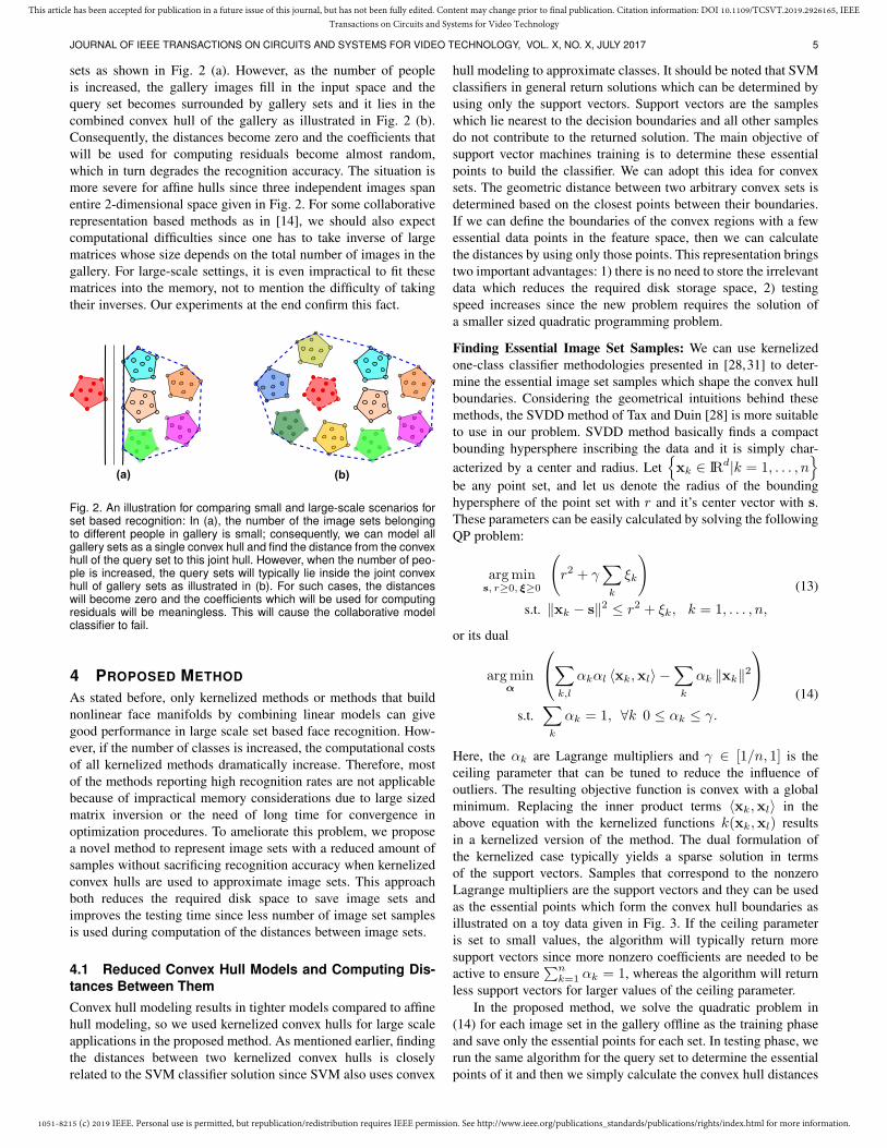
sets as shown in Fig. 2 (a). However, as the number of people

is increased, the gallery images fill in the input space and the

query set becomes surrounded by gallery sets and it lies in the

combined convex hull of the gallery as illustrated in Fig. 2 (b).

Consequently, the distances become zero and the coefficients that

will be used for computing residuals become almost random,

which in turn degrades the recognition accuracy. The situation is

more severe for affine hulls since three independent images span

entire 2-dimensional space given in Fig. 2. For some collaborative

representation based methods as in [14], we should also expect

computational difficulties since one has to take inverse of large

matrices whose size depends on the total number of images in the

gallery. For large-scale settings, it is even impractical to fit these

matrices into the memory, not to mention the difficulty of taking

their inverses. Our experiments at the end confirm this fact.

(a) (b)

Fig. 2. An illustration for comparing small and large-scale scenarios forset based recognition: In (a), the number of the image sets belongingto different people in gallery is small; consequently, we can model allgallery sets as a single convex hull and find the distance from the convexhull of the query set to this joint hull. However, when the number of peo-ple is increased, the query sets will typically lie inside the joint convexhull of gallery sets as illustrated in (b). For such cases, the distanceswill become zero and the coefficients which will be used for computingresiduals will be meaningless. This will cause the collaborative modelclassifier to fail.

4 PROPOSED METHOD

As stated before, only kernelized methods or methods that build

nonlinear face manifolds by combining linear models can give

good performance in large scale set based face recognition. How-

ever, if the number of classes is increased, the computational costs

of all kernelized methods dramatically increase. Therefore, most

of the methods reporting high recognition rates are not applicable

because of impractical memory considerations due to large sized

matrix inversion or the need of long time for convergence in

optimization procedures. To ameliorate this problem, we propose

a novel method to represent image sets with a reduced amount of

samples without sacrificing recognition accuracy when kernelized

convex hulls are used to approximate image sets. This approach

both reduces the required disk space to save image sets and

improves the testing time since less number of image set samples

is used during computation of the distances between image sets.

4.1 Reduced Convex Hull Models and Computing Dis-

tances Between Them

Convex hull modeling results in tighter models compared to affine

hull modeling, so we used kernelized convex hulls for large scale

applications in the proposed method. As mentioned earlier, finding

the distances between two kernelized convex hulls is closely

related to the SVM classifier solution since SVM also uses convex

hull modeling to approximate classes. It should be noted that SVM

classifiers in general return solutions which can be determined by

using only the support vectors. Support vectors are the samples

which lie nearest to the decision boundaries and all other samples

do not contribute to the returned solution. The main objective of

support vector machines training is to determine these essential

points to build the classifier. We can adopt this idea for convex

sets. The geometric distance between two arbitrary convex sets is

determined based on the closest points between their boundaries.

If we can define the boundaries of the convex regions with a few

essential data points in the feature space, then we can calculate

the distances by using only those points. This representation brings

two important advantages: 1) there is no need to store the irrelevant

data which reduces the required disk storage space, 2) testing

speed increases since the new problem requires the solution of

a smaller sized quadratic programming problem.

Finding Essential Image Set Samples: We can use kernelized

one-class classifier methodologies presented in [28,31] to deter-

mine the essential image set samples which shape the convex hull

boundaries. Considering the geometrical intuitions behind these

methods, the SVDD method of Tax and Duin [28] is more suitable

to use in our problem. SVDD method basically finds a compact

bounding hypersphere inscribing the data and it is simply char-

acterized by a center and radius. Let{

xk ∈ IRd|k = 1, . . . , n}

be any point set, and let us denote the radius of the bounding

hypersphere of the point set with r and it’s center vector with s.

These parameters can be easily calculated by solving the following

QP problem:

argmins, r≥0, ξ≥0

(

r2 + γ∑

k

ξk

)

s.t. ‖xk − s‖2 ≤ r2 + ξk, k = 1, . . . , n,

(13)

or its dual

argminα

∑

k,l

αkαl 〈xk,xl〉 −∑

k

αk ‖xk‖2

s.t.∑

k

αk = 1, ∀k 0 ≤ αk ≤ γ.

(14)

Here, the αk are Lagrange multipliers and γ ∈ [1/n, 1] is the

ceiling parameter that can be tuned to reduce the influence of

outliers. The resulting objective function is convex with a global

minimum. Replacing the inner product terms 〈xk,xl〉 in the

above equation with the kernelized functions k(xk,xl) results

in a kernelized version of the method. The dual formulation of

the kernelized case typically yields a sparse solution in terms

of the support vectors. Samples that correspond to the nonzero

Lagrange multipliers are the support vectors and they can be used

as the essential points which form the convex hull boundaries as

illustrated on a toy data given in Fig. 3. If the ceiling parameter

is set to small values, the algorithm will typically return more

support vectors since more nonzero coefficients are needed to be

active to ensure∑n

k=1αk = 1, whereas the algorithm will return

less support vectors for larger values of the ceiling parameter.

In the proposed method, we solve the quadratic problem in

(14) for each image set in the gallery offline as the training phase

and save only the essential points for each set. In testing phase, we

run the same algorithm for the query set to determine the essential

points of it and then we simply calculate the convex hull distances





-12 -10 -8 -6 -4 -2 0 2 4-12

-10

-8

-6

-4

-2

0

2

4

6

Fig. 3. Nonlinearly distributed toy data (shown with blue crosses) andthe support vectors (shown with red circles around the data samples)returned by SVDD using a Gaussian kernel. Support vectors lie close tothe object boundaries when the Gaussian kernel width is set properly.

between the query set and gallery sets. Here, set-to-set distances

are computed by using only the essential points which constitute

a small part of the entire data. In this methodology, testing time

is improved because of solving smaller sized quadratic problems

and the amount of data is reduced without any significant decrease

in the accuracy. We call this methodology as the Reduced Convex

Hull based Image Set Distance (RCHISD) method.

Using Hypersphere Models for Image Set Classification: An-

other basic strategy for modeling image sets can be using hyper-

spheres. The geometric distance between two hyperspheres can be

calculated by using only their radii and centers. When the gallery

and query sets are modeled in terms of kernelized hyperspheres,

this representation will be convenient due to the easiness in set-to-

set distance calculations. The center of the kernelized hypersphere

model of the c-th class can be found as given in the following:

sc =∑

k

α∗ckxck. (15)

Here, α∗c are the nonzero coefficients returned by the quadratic

programming solver, and the radius of the model is given by rc =||xck − sc|| for any xck for which 0 < α∗

ck < γ. Finally, if

hsc and hsc′ (characterized by their center and radius) are two

kernelized hyperspheres, the geometric distance between them can

be computed easily as:

d(hsc, hsc′) = ||sc − sc′ || − (rc + rc′), (16)

where

||sc − sc′ || =√

∑

i,j αciαcj 〈xci,xcj〉 − 2∑

i,k αciαc′k 〈xci,xc′k〉+∑

k,l αc′kαc′l 〈xc′k,xc′l〉.

In this representation, using a few support vectors corresponding

to the nonzero Lagrange multipliers will be enough to calculate

the distances. To the best of our knowledge, this is the first time

hypersphere models have been used for image set classification.

Setting Design Parameters for Reducing Image Sets: There

are two design parameters in kernelized representations of the

proposed methods. The first parameter is the ceiling parameter

(γ), and the accuracy is not very sensitive to it as demonstrated

in the experimental work. The second parameter is the Gaussian

kernel width σ, and the number of reduced samples is completely

determined by σ. Using a higher value results in less number

of returned samples as indicated in Fig. 4. In this example, we

have demonstrated that using different values of Gaussian kernel

width yields different amount of essential samples. The more

number of reduced samples achieves better recognition rates but

less number of reduced data yields faster testing. Since there is

a trade-off between the accuracy and the real time performance,

this parameter should be adjusted properly. The best parameter

can result in significant improvements in storage and testing times

with an inconsiderable decrease in accuracy.

Fig. 4. An example on a toy data to demonstrate the effect of Gaussiankernel width in reduced convex hull modeling. Red circles are thesupport vectors returned by SVDD algorithm when the Gaussian kernelwidth is set to: (a) σ =1.5, (b) σ =2.0, (c) σ =2.5, (d) σ =3.5, (e)σ =4.5, (f) σ =5.0.

4.2 Speed Improvement by Using Binary Hierarchical

Decision Trees for Image Set Based Recognition

Once we determine the essential data samples to represent image

sets, we find the distances between the query set and each set

in the gallery. This can be implemented in parallel since the

individual set distances between a query and gallery sets are

independent. In addition, we propose another approach to speed

up the classification of the query set below.

When we consider individual comparisons between a query set

and each gallery set, some of the comparisons may be unnecessary

for a classification of a particular query. For instance, if query set

belongs to a male subject, it may be further from many image

sets belonging to female subjects in the gallery. Similarly, for set

based general visual object classification tasks, if the query set

belongs to a dog class, it is somewhat unnecessary to making

comparisons between unrelated classes such as aeroplanes, cars,

etc.. In order to avoid such unnecessary comparisons and to speed

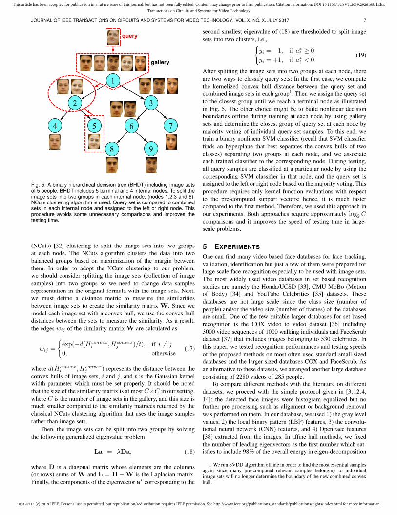
up the classification process, we can use a binary hierarchical

decision tree (BHDT) that splits the sets in the gallery into two

groups until reaching a single set for each group. In this case, one

needs to make less number of comparisons between the query and

the gallery; because traversing a path from the top to a bottom

node takes less time for decision making as illustrated in Fig.

5. When C denotes the number of person classes, this requires

approximately log2C comparisons in contrast to C comparisons

which in turn may significantly improve the testing time.

In this setup, both the accuracy and speed depend on the tree-

structure that creates well-balanced separable image class groups

at each node of the tree. To this end, we used the Normalized Cuts





1

2 3

5 64 7

8 9

query

gallery

Fig. 5. A binary hierarchical decision tree (BHDT) including image setsof 5 people. BHDT includes 5 terminal and 4 internal nodes. To split theimage sets into two groups in each internal node, (nodes 1,2,3 and 6),NCuts clustering algorithm is used. Query set is compared to combinedsets in each internal node and assigned to the left or right node. Thisprocedure avoids some unnecessary comparisons and improves thetesting time.

(NCuts) [32] clustering to split the image sets into two groups

at each node. The NCuts algorithm clusters the data into two

balanced groups based on maximization of the margin between

them. In order to adopt the NCuts clustering to our problem,

we should consider splitting the image sets (collection of image

samples) into two groups so we need to change data samples

representation in the original formula with the image sets. Next,

we must define a distance metric to measure the similarities

between image sets to create the similarity matrix W. Since we

model each image set with a convex hull, we use the convex hull

distances between the sets to measure the similarity. As a result,

the edges wij of the similarity matrix W are calculated as

wij =

{

exp(−d(Hconvexi , Hconvex

j )/t), if i 6= j

0, otherwise(17)

where d(Hconvexi , Hconvex

j ) represents the distance between the

convex hulls of image sets, i and j, and t is the Gaussian kernel

width parameter which must be set properly. It should be noted

that the size of the similarity matrix is at most C×C in our setting,

where C is the number of image sets in the gallery, and this size is

much smaller compared to the similarity matrices returned by the

classical NCuts clustering algorithm that uses the image samples

rather than image sets.

Then, the image sets can be split into two groups by solving

the following generalized eigenvalue problem

La = λDa, (18)

where D is a diagonal matrix whose elements are the columns

(or rows) sums of W and L = D −W is the Laplacian matrix.

Finally, the components of the eigenvector a∗ corresponding to the

second smallest eigenvalue of (18) are thresholded to split image

sets into two clusters, i.e.,{

yi = −1, if a∗i ≥ 0

yi = +1, if a∗i < 0(19)

After splitting the image sets into two groups at each node, there

are two ways to classify query sets: In the first case, we compute

the kernelized convex hull distance between the query set and

combined image sets in each group1. Then we assign the query set

to the closest group until we reach a terminal node as illustrated

in Fig. 5. The other choice might be to build nonlinear decision

boundaries offline during training at each node by using gallery

sets and determine the closest group of query set at each node by

majority voting of individual query set samples. To this end, we

train a binary nonlinear SVM classifier (recall that SVM classifier

finds an hyperplane that best separates the convex hulls of two

classes) separating two groups at each node, and we associate

each trained classifier to the corresponding node. During testing,

all query samples are classified at a particular node by using the

corresponding SVM classifier in that node, and the query set is

assigned to the left or right node based on the majority voting. This

procedure requires only kernel function evaluations with respect

to the pre-computed support vectors; hence, it is much faster

compared to the first method. Therefore, we used this approach in

our experiments. Both approaches require approximately log2C

comparisons and it improves the speed of testing time in large-

scale problems.

5 EXPERIMENTS

One can find many video based face databases for face tracking,

validation, identification but just a few of them were prepared for

large scale face recognition especially to be used with image sets.

The most widely used video databases in set based recognition

studies are namely the Honda/UCSD [33], CMU MoBo (Motion

of Body) [34] and YouTube Celebrities [35] datasets. These

databases are not large scale since the class size (number of

people) and/or the video size (number of frames) of the databases

are small. One of the few suitable larger databases for set based

recognition is the COX video to video dataset [36] including

3000 video sequences of 1000 walking individuals and FaceScrub

dataset [37] that includes images belonging to 530 celebrities. In

this paper, we tested recognition performances and testing speeds

of the proposed methods on most often used standard small sized

databases and the larger sized databases COX and FaceScrub. As

an alternative to these datasets, we arranged another large database

consisting of 2280 videos of 285 people.

To compare different methods with the literature on different

datasets, we proceed with the simple protocol given in [3,12,4,

14]: the detected face images were histogram equalized but no

further pre-processing such as alignment or background removal

was performed on them. In our database, we used 1) the gray level

values, 2) the local binary pattern (LBP) features, 3) the convolu-

tional neural network (CNN) features, and 4) OpenFace features

[38] extracted from the images. In affine hull methods, we fixed

the number of leading eigenvectors as the first number which sat-

isfies to include 98% of the overall energy in eigen-decomposition

1. We run SVDD algorithm offline in order to find the most essential samplesagain since many pre-computed relevant samples belonging to individualimage sets will no longer determine the boundary of the new combined convexhull.





stage. In the kernelized methods we used the Gaussian kernel

functions and the width parameter is determined empirically by

using randomly selected subsets of each image sets. We compared

the proposed method RCHISD and its fast version using BHDT

(RCHISD-BHDT), to the linear/kernelized convex hull method

(CHISD) [3], linear/kernelized affine hull method (AHISD) [3],

SANP [11], Mutual Subspace Method (MSM) [5], Regularized

Nearest Points (RNP) [12], Manifold-Manifold Distance (MMD)

[4], Collaboratively Regularized Nearest Points(CRNP) [14] and

Self-Regularized Nonnegative Adaptive Distance Metric Learning

(SRN-ADML) [39]. In addition to these methods, we also tested

linear/kernelized bounding hypersphere (HS) models for image set

classification. All image sets and their extracted features used in

this work as well as codes of our new methods are available at

http://mlcv.ogu.edu.tr/softwares.html.

5.1 Experiments on Small Sized Data Sets

5.1.1 Experiments on Honda/UCSD Data Set

The Honda/UCSD dataset is one of the most used databases in

set based recognition studies. It consists of 20 individuals and 59

video sequences with each sequence including approximately 300-

500 frames. The detected faces were histogram equalized and the

resulting re-sized gray scale pixel values were used as features.

In the experiment, 20 sequences set aside for training are used as

the gallery image sets and the remaining 39 sequences are used

in testing. We did not extract LBP or CNNs for this dataset since

gray level values already achieved very high accuracies.

The experimental results are given in Table 1. Here, the testing

time corresponds to the time spent to classify a single test set

on the average. In this experiment, the ceiling parameter of the

kernelized convex hull method is changed from 0.1 to 1, and we

achieved the highest recognition accuracies (100%) for all cases.

Using reduced amount of samples did not affect the accuracy in

any way and it improved testing times. RCHISD testing time

is approximately 2 times faster than the traditional kernelized

CHISD. Similarly, RCHISD+BHDT improves the testing time

more and it is approximately 6.3 times faster than the traditional

kernelized CHISD. Regarding the improvements in storage, the

total number of face images in all sets was 14050 and it is

reduced to 4279 in RCHISD without any drop in accuracy. In this

experiment, RNP, CRNP, MMD, kernel CHISD, RCHISD, and

RCHISD-BHDT methods all achieve 100% recognition accuracy.

The worst performing method is the linear hyperspheres but it

is the fastest method among all. The slowest methods are kernel

AHISD in kernelized methods and SANP in linear methods. It

should be noted that there is no big accuracy difference between

the linear and kernelized methods except for the hypersphere

classifier mostly because of the number of people in the dataset is

small.

5.1.2 Experiments on MoBo Data Set

The MoBo (Motion of the Body) dataset contains 96 image

sequences of 24 individuals walking on a treadmill. Images were

collected from multiple cameras, and each image set includes both

frontal and profile views of the subject’s faces. For this database,

we used LBP features from [3].

The experimental setup has been prepared the same way as

given in [3]. In this setup, we randomly select one set from each

class and use it in the gallery and the remaining 3 sets are used in

testing. This process is repeated 10 times and we report the average

TABLE 1Classification Rates (%) and Testing Times on the Honda/UCSD

Dataset.

Method Accuracy Testing Time (sec)

Linear AHISD 97.4 1.6 sec

Linear CHISD 97.4 5.1 sec

Linear HS 59.0 0.6 sec

MSM 97.4 2.2 sec

SANP 97.4 16.7 sec

RNP 100 5.4 sec

CRNP 100 2.6 sec

SRN-ADML 97.4 6.2 sec

MMD 100 7.1 sec

Kernel AHISD 97.4 14.2 sec

Kernel CHISD 100 7.6 sec

Kernel HS 94.9 2.8 sec

Kernel RCHISD 100 3.7 sec

Kernel RCHISD-BHDT 100 1.2 sec

TABLE 2Classification Rates (%) and Testing Times on the MoBo Dataset.


Linear AHISD 95.3± 2.6 32.0 sec

Linear CHISD 98.1± 0.9 25.6 sec

Linear HS 71.9± 4.7 0.6 sec

MSM 92.4± 1.9 9.2 sec

SANP 98.1± 0.9 40.2 sec

RNP 93.8± 2.7 11.3 sec

CRNP 97.4± 0.8 15.8 sec

SRN-ADML 95.3± 1.6 30.0 sec

MMD 94.7± 2.3 10.6 sec

Kernel AHISD 96.4± 2.5 87.3 sec

Kernel CHISD 98.1± 0.9 32.8 sec

Kernel HS 87.8± 2.8 5.8 sec

Kernel RCHISD 97.3± 1.3 8.3 sec

Kernel RCHISD-BHDT 95.6± 1.8 3.2 sec

classification rates over the 10 runs. The ceiling parameter for the

RCHISD method has been tested in the range γ ∈ [0.1, 1] and

all of them returned the same accuracies. Therefore, we conclude

that the results are not sensitive to this parameter so we fixed it as

γ = 0.2 for the rest of the experiments. Experimental results are

given in Table 2.

In this experiment, the linear and kernelized convex hull mod-

els with SANP method give the best accuracies. Using RCHISD

results in a 0.8% decrease in accuracy but it completes testing

approximately 4 times faster than kernel CHISD and 4.8 times

faster than SANP methods. Therefore reducing the image sets

samples significantly improves testing times without much drop

in accuracy. Similarly, RCHISD-BHDT is 2.6 times faster than

RCHISD but it results in a 2.5% decrease in average recognition

rate. The fastest method is the linear hypersphere method but it

gives the worst recognition rate. In regard to the data reduction,

RCHISD reduces the number of images in the sets from 48789

to 7098 which is a good improvement in storage. The accuracy

difference between the linear and kernelized methods are not high

except for the hypersphere classifier as in the previous case.

5.1.3 Experiments on YouTube Celebrities Data Set

The YouTube Celebrities data set contains 1910 videos of 47

celebrities that are collected from YouTube. Each sequence in-

cludes different number of frames that are mostly low resolution.





The data set does not provide the cropped faces from videos.

Therefore, we manually cropped faces using a semi-automatic

annotation tool and resized them to 40×40 gray-scale images. We

conduct 10 runs of experiments by randomly selecting 9 videos (3

for training, 6 for testing) for each experiment by following the

same protocol of [15,20]. The averages of the classification rates

and testing times are shown in Table 3.

TABLE 3Classification Rates (%) and Testing Times on the YouTube Celebrities

Dataset.


Linear AHISD 51.1± 2.8 1.2 sec

Linear CHISD 57.8± 2.7 7.5 sec

Linear HS 39.0± 2.9 0.8 sec

MSM 50.5± 3.1 14.4 sec

SANP 51.6± 4.0 39.5 sec

RNP 61.3± 2.5 21.4 sec

CRNP 56.7± 0.5 2.8 sec

SRN-ADML 55.1± 2.7 27.8 sec

MMD 59.8± 3.6 11.9 sec

Kernel AHISD 57.4± 1.9 24.8 sec

Kernel CHISD 58.2± 2.6 25.6 sec

Kernel HS 44.0± 2.9 1.7 sec

Kernel RCHISD 57.2± 2.7 4.8 sec

Kernel RCHISD-BHDT 55.6± 2.1 3.1 sec

The videos in this dataset mostly include frontal views of peo-

ple; therefore, linear methods perform well here. In particular, the

best accuracy is obtained by RNP which is a linear method. Kernel

CHISD achieves the second best result. Using reduced image sets

slightly decreases the performance, but it is approximately 5.3

times faster compared to using full data. Using BHDT improves

the testing time a little bit more, but the accuracy also drops around

1.6%. SANP method is the worst performing method in terms of

speed as in the previous cases.

5.2 Experiments on Larger Sized Data Sets

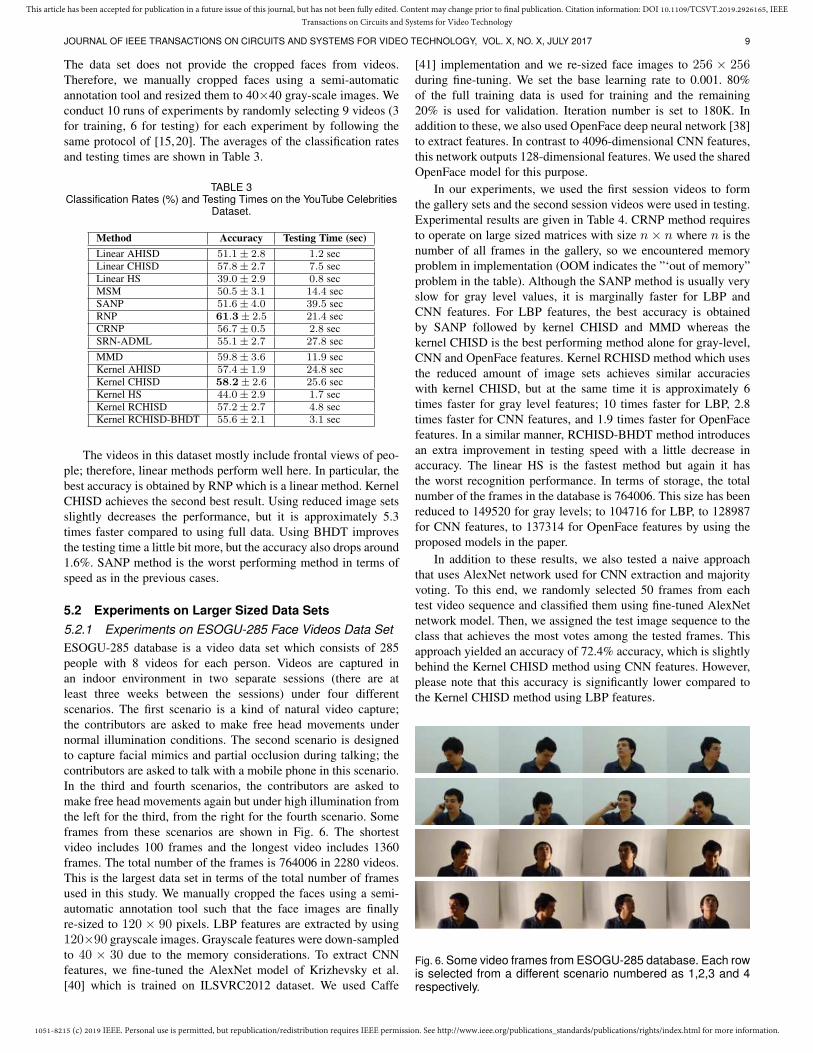
5.2.1 Experiments on ESOGU-285 Face Videos Data Set

ESOGU-285 database is a video data set which consists of 285

people with 8 videos for each person. Videos are captured in

an indoor environment in two separate sessions (there are at

least three weeks between the sessions) under four different

scenarios. The first scenario is a kind of natural video capture;

the contributors are asked to make free head movements under

normal illumination conditions. The second scenario is designed

to capture facial mimics and partial occlusion during talking; the

contributors are asked to talk with a mobile phone in this scenario.

In the third and fourth scenarios, the contributors are asked to

make free head movements again but under high illumination from

the left for the third, from the right for the fourth scenario. Some

frames from these scenarios are shown in Fig. 6. The shortest

video includes 100 frames and the longest video includes 1360

frames. The total number of the frames is 764006 in 2280 videos.

This is the largest data set in terms of the total number of frames

used in this study. We manually cropped the faces using a semi-

automatic annotation tool such that the face images are finally

re-sized to 120 × 90 pixels. LBP features are extracted by using

120×90 grayscale images. Grayscale features were down-sampled

to 40 × 30 due to the memory considerations. To extract CNN

features, we fine-tuned the AlexNet model of Krizhevsky et al.

[40] which is trained on ILSVRC2012 dataset. We used Caffe

[41] implementation and we re-sized face images to 256 × 256during fine-tuning. We set the base learning rate to 0.001. 80%

of the full training data is used for training and the remaining

20% is used for validation. Iteration number is set to 180K. In

addition to these, we also used OpenFace deep neural network [38]

to extract features. In contrast to 4096-dimensional CNN features,

this network outputs 128-dimensional features. We used the shared

OpenFace model for this purpose.

In our experiments, we used the first session videos to form

the gallery sets and the second session videos were used in testing.

Experimental results are given in Table 4. CRNP method requires

to operate on large sized matrices with size n× n where n is the

number of all frames in the gallery, so we encountered memory

problem in implementation (OOM indicates the ”‘out of memory”

problem in the table). Although the SANP method is usually very

slow for gray level values, it is marginally faster for LBP and

CNN features. For LBP features, the best accuracy is obtained

by SANP followed by kernel CHISD and MMD whereas the

kernel CHISD is the best performing method alone for gray-level,

CNN and OpenFace features. Kernel RCHISD method which uses

the reduced amount of image sets achieves similar accuracies

with kernel CHISD, but at the same time it is approximately 6

times faster for gray level features; 10 times faster for LBP, 2.8

times faster for CNN features, and 1.9 times faster for OpenFace

features. In a similar manner, RCHISD-BHDT method introduces

an extra improvement in testing speed with a little decrease in

accuracy. The linear HS is the fastest method but again it has

the worst recognition performance. In terms of storage, the total

number of the frames in the database is 764006. This size has been

reduced to 149520 for gray levels; to 104716 for LBP, to 128987

for CNN features, to 137314 for OpenFace features by using the

proposed models in the paper.

In addition to these results, we also tested a naive approach

that uses AlexNet network used for CNN extraction and majority

voting. To this end, we randomly selected 50 frames from each

test video sequence and classified them using fine-tuned AlexNet

network model. Then, we assigned the test image sequence to the

class that achieves the most votes among the tested frames. This

approach yielded an accuracy of 72.4% accuracy, which is slightly

behind the Kernel CHISD method using CNN features. However,

please note that this accuracy is significantly lower compared to

the Kernel CHISD method using LBP features.

Fig. 6. Some video frames from ESOGU-285 database. Each rowis selected from a different scenario numbered as 1,2,3 and 4respectively.





TABLE 4Classification Rates (%) and Testing Times on ESOGU-285 Video Dataset.

MethodsGrayscale Values LBP Features CNN Features OpenFace Features

Accuracy Testing Time Accuracy Testing Time Accuracy Testing Time Accuracy Testing Time

Linear AHISD 44.3 22.0 sec 66.8 180.0 sec 65.0 543.8 sec 60.9 2.8 sec

Linear CHISD 55.1 179.6 sec 76.6 390.1 sec 65.1 378.6 sec 45.9 57.8 sec

Linear HS 29.0 3.9 sec 39.5 0.8 sec 33.2 3.2 sec 26.3 0.03 sec

MSM 50.1 2.3 sec 69.6 5.1 sec 63.5 5.6 sec 44.8 1.28 sec

SANP 51.9 29771.0 sec 79.1 564.6 sec 69.4 1087.6 sec 52.2 7.1 sec

RNP 46.7 1731.7 sec 51.9 2205.3 sec 71.7 367.8 sec 35.6 23.1 sec

CRNP OOM − OOM − OOM − OOM −

SRN-ADML 45.4 364.6 sec 68.4 380.2 sec 57.0 458.5 sec 31.2 20.2 sec

MMD 52.0 7.2 sec 77.6 30.4 sec 69.8 28.9 sec 52.2 1.8 sec

Kernel AHISD 62.1 2015.0 sec 76.1 4369.0 sec 72.5 357.7 sec 71.0 746.4 sec

Kernel CHISD 62.1 233.3 sec 77.6 480.4 sec 72.8 156.8 sec 71.7 84.2 sec

Kernel HS 43.7 61.9 sec 49.4 12.9 sec 48.5 9.5 sec 46.4 7.9 sec

Kernel RCHISD 61.2 39.7 sec 75.4 46.1 sec 71.7 55.6 sec 70.0 44.7 sec

Kernel RCHISD-BHDT 60.8 20.6 sec 73.3 24.1 sec 70.2 25.6 sec 62.9 22.9 sec

TABLE 5Classification Rates (%) and Testing Times on the COX Dataset.

MethodsGrayscale Values LBP Features

Accuracy Testing Time Accuracy Testing Time

Linear AHISD 42.4± 7.6 71.3 sec 44.3± 9.8 82.9 sec

Linear CHISD 42.8± 13.2 42.9 sec 44.8± 11.3 54.3 sec

Linear HS 16.5± 4.2 0.9 sec 25.1± 4.9 1.5 sec

MSM 40.6± 10.2 17.3 sec 41.6± 5.3 18.6 sec

SANP 41.7± 10.3 1856.5 sec 43.6± 11.2 978.7 sec

RNP 42.5± 11.3 594.3 sec 45.4± 13.7 217.3 sec

CRNP OOM −− OOM −−

SRN-ADML 42.7± 10.8 354.7 sec 44.6± 7.9 351.7 sec

MMD 33.6± 8.8 42.9 sec 42.7± 10.5 60.3 sec

Kernel AHISD 43.2± 12.3 259.9 sec 45.4± 10.3 276.4 sec

Kernel CHISD 43.9± 13.0 222.9 sec 45.6± 10.9 250.2 sec

Kernel HS 20.7± 6.3 4.5 sec 42.4± 7.6 71.3 sec

Kernel RCHISD 41.9± 11.7 39.6 sec 44.3± 11.5 65.2 sec

Kernel RCHISD-BHDT 40.7± 13.4 22.7 sec 41.6± 10.2 30.6 sec

In ESOGU-285 database, there is a big difference in correct

recognition rates between the linear methods and their kernelized

counterparts especially for gray level values and OpenFace fea-

tures in contrast to the experimental results obtained on small

sized datasets. The accuracy difference between the linear and

kernelized affine hull methods is 17.8% whereas the difference

between linear and kernelized convex hulls is 7% for gray levels.

Similarly, for OpenFace features, the accuracy difference between

the linear and kernelized affine hull methods is 10.1%, and the

difference between linear and kernelized convex hulls is 25.8%.

However, for LBP features, there is still a big difference (9.3%)

between the linear and kernelized affine hull models but there is

a slight difference (1%) between the linear and kernelized convex

hull models. Since convex hulls are much tighter models than

the affine hulls, this result indicates that LBP features are more

discriminative features compared to gray level values and they

yield to more compact face manifolds. LBP features also yield to

better results compared to CNNs, but the performance difference is

not very significant as in gray level values. The accuracies of linear

methods using OpenFace features are very low compared to the

ones using CNN features, but the accuracies of nonlinear methods

are similar for both CNN and OpenFace features. We believe that

this is due to fact that CNN and OpenFace features of frontal,

left and right profile views are quite different and the resulting

image feature sets can be seen as kind of mixture of Gaussians

where each component lie in isolated region of feature space (as

opposed to a smooth nonlinear manifold). As a result, the linear

models cannot approximate this structure well whereas kernel

methods can successfully approximate this nonlinear model. In a

similar manner, a naive approach using fine-tuned AlexNet model

and majority voting yielded an accuracy lower than the proposed

methods. We believe that the classical deep neural network based

methods trained with single images will not work well for set

based recognition where the images have different poses including

full left/right profile views in addition to the frontal views. Instead,

we must train such nets with image sets and enforce to minimize

the distances between the different pose image features in the same

set (by using Siamese or Triplet network type network structures)

to obtain higher accuracies.

5.2.2 Experiments on COX Video to Video Data Set

The COX Faces dataset is a new dataset, which contains 3000

video sequences of 1000 walking individuals [36]. The videos

are captured with three fixed camcorders when the subjects walk

around the pre-designed S-shape route. The dataset has variations

in illumination, pose and resolution through this S-shape route.

For this database we used 32×40 histogram equalized face image

gray-scale values and LBP features (LBP features are extracted

from 32×40 face images since we do not have access to original





TABLE 6Classification Rates (%) and Testing Times on the FaceScrub Dataset.

MethodsLBP Features CNN Features

Accuracy Testing Time Accuracy Testing Time

Linear AHISD 98.3± 0.3 2.1 sec 99.94± 0.05 6.17 sec

Linear CHISD 98.2± 0.3 9.2 sec 99.97± 0.04 8.33 sec

Linear HS 32.7± 1.2 0.01 sec 99.94± 0.05 0.06 sec

MSM 98.1± 0.3 0.1 sec 99.94± 0.05 0.30 sec

SANP 92.7± 0.6 20.5 sec 99.94± 0.05 75.40 sec

RNP 99.6± 0.1 41.3 sec 100± 0.00 10.81 sec

CRNP OOM −− OOM −−

SRN-ADML 97.4± 0.5 21.7 sec 99.95± 0.04 14.78 sec

MMD 89.7± 0.7 0.5 sec 100± 0.00 2.45 sec

Kernel AHISD 98.3± 0.3 12.9 sec 99.98± 0.03 76.30 sec

Kernel CHISD 98.4± 0.4 13.6 sec 100± 0.00 42.90 sec

Kernel HS 53.6± 1.4 2.2 sec 100± 0.00 2.11 sec

Kernel RCHISD 97.1± 0.7 7.4 sec 100± 0.00 20.30 sec

Kernel RCHISD-BHDT 95.1± 0.7 5.9 sec 99.77± 0.18 4.10 sec

video frames) as visual features. We did not extract CNN features

because of the small size of the face images. There are 3 image

sets per person. We choose one set from each person for testing

and the remaining two sets were used as gallery. For the second

and the third trials, we have chosen the test set from the ones that

were not used for testing earlier.

The classification rates are the averages of these three trials,

and they are given in Table 5. We could not implement CRNP,

because of memory issues as before since it has to operate on a

large matrix. As opposed to the experiments on ESOGU faces,

there are not significant differences between accuracies obtained

by gray-scale values and LBP features, because LBP features are

extracted from small 32×40 face images (the authors [36] share

only these small cropped face images). The best classification

accuracies are obtained by linear and kernelized CHISD methods.

Using reduced convex hulls decreases the performance by around

2%, but the speed is 5.6 times faster compared to using full data for

gray-scale values. Similarly, using reduced convex hulls decreases

the performance by 1.3%, but the speed is 3.8 times faster for

LBP features. The kernelized RCHISD method using BHDT is

approximately 9.8 times faster compared to using full image sets

for gray-scale values and 8.2 times faster for LBP features. SANP

is again the slowest method. The total number of face image

frames is 412415 and it is decreased to 41461 for gray-scale values

and to 50976 for LBP features by using the proposed reduction

method.

5.2.3 Experiments on FaceScrub Data Set

FaceScrub dataset [37] includes face images of 530 celebrities. It

has been created by detecting faces based on automated search

of public figures on the internet followed by manually checking

and cleaning the results. In the dataset, there are 265 male and

265 female celebrities’ face images whose internet links and face

coordinates are given in a text file. The file includes over 100,000

face image links but some links belong to forbidden or not found

web pages. First, we downloaded the dataset and cropped the

faces by using the information in the supplied text file. Then, we

manually checked the face images and cleaned non-face images

since there were still some annotation mistakes. As a result, we

had 67,437 face images of 530 celebrities with an average of 127

images (minimum 39, maximum 201) per person which is suitable

to form image sets. The face images are mostly high resolution

frontal face images and we resized them to 128×128. Some of the

images are given in Fig. 7. Similar to the other experiments, we

extracted LBP and CNN features of images.

Fig. 7. Some face image samples from FaceScrub Dataset.

In our tests, we first divided the dataset into 4 equal folds,

and we used the images of one fold as gallery and the remaining

images are used for testing (i.e., 530 image sets are used as gallery

set and the remaining 3×530=1590 image sets are used as test

set). This is repeated 4 times for each fold and the final accuracy

is the average of the results obtained in each trial. The results

are given in Table 6. As can be seen in the results, majority of

the tested methods achieve very high accuracies owing the fact

that the images were mostly frontal and high quality images.

As opposed to ESOGU experiments, CNN features yield higher

accuracies than LBP features. It should be noted that even the

worst performing linear hyperspheres method among all tested

methods also achieves a very high accuracy for CNN features. This

clearly shows that CNN features of all images in the same sets are

very compact for this dataset and it can be easily modeled with

simple models like a linear hypersphere. For LBP features, the

best accuracies are obtained by RNP among linear methods and by

Kernel CHISD method among nonlinear methods. For CNN fea-

tures almost all tested methods achieve very high accuracies close

to 100%. The proposed reduction method, Kernel RCHISD, is 1.8

times faster compared to Kernel CHISD, and it is approximately

2.1 times faster for CNN features. The proposed method using

binary hierarchical trees improves the testing time even more as

in the other experiments. In terms of data reduction, the proposed

reduction method decreases the total number of images in the

entire dataset, 67437, to 35623 for LBP features and to 28272

for CNN features with only a minor drop in the classification





accuracy.

6 CONCLUSION

In this work, we developed image set based classification methods

which use the reduced amount of image samples in each set to

lessen the required disk space and speed up the testing process for

large scale face recognition systems. To this end, image sets are

approximated with kernelized convex hulls and the set boundaries

are determined based on the compact hypersphere returned by

SVDD method. We call the new representation as the reduced

convex hull based image set distance. The method inherently

reduces the required storage, because only the samples that form

the image set boundaries were kept as the essential data and

there is no need to store the rest of the samples of the same set.

Experimental results verify that reducing image set samples via

SVDD also greatly improves the testing time without a significant

drop in accuracy.

Beyond the proposed methods, we also investigated the hyper-

sphere models to approximate the image sets. Experiments showed

that hypersphere models provide extremely faster classification but

they result in much lower recognition rates compared to affine hull

or convex hull models. Therefore, it is not wise to use hypersphere

models in final decision but they can be appropriately used to

return some nearest approximate candidates from the gallery set

rapidly, then a more efficient method can be used to classify the

returned candidates.

Lastly, it should be noted that there is an obvious difference

in recognition rates of the linear methods and their kernelized

counterparts between the applications of them in small and large

sized data sets. The accuracies of linear methods used for image

set representations drop as the number of classes is increased.

Especially, when looser linear models (such as affine hulls or

linear subspaces) are used to represent the image sets, a serious

drop has been observed. In this work, we also verified that some

recently proposed methods reporting high recognition accuracies

[11,14] cannot be applied to a large sized data (even to moderate

size data like our dataset) because of their slow testing speed or

memory problems.

ACKNOWLEDGMENTS

This work was supported by the Scientific and Technological

Research Council of Turkey (TUBITAK) with Grant number

TUBITAK-114E014.

REFERENCES

[1] O. Arandjelovic, G. Shakhnarovich, J. Fisher, R. Cipolla, T.

Darrell, Face Recognition with Image Sets Using Manifold

Density Divergence, IEEE Computer Society Conference on

Computer Vision and Pattern Recognition, 2005.

[2] Gregory Shakhnarovich, John W. Fisher, Trevor Darrell, Face

Recognition from Long-Term Observations, European Confer-

ence on Computer Vision, 2002.

[3] H. Cevikalp, B. Triggs, Face recognition based on image sets,

IEEE Computer Society Conference on Computer Vision and

Pattern Recognition, 2010.

[4] R. Wang, S. Shan, X. Chen, W. Gao, Manifold-Manifold

Distance with application to face recognition based on image

set, IEEE Computer Society Conference on Computer Vision

and Pattern Recognition, 2008.

[5] O. Yamaguchi, E. Fukui, K. Maeda, Face recognition using

temporal image sequence, IEEE International Conference on

Automatic Face and Gesture Recognition, 1998.

[6] J. Hamm, D. D. Lee, Grassmann Discriminant Analysis:

A Unifying View on Subspace-based Learning, International

Conference on Machine Learning, 2008.

[7] T. Wang, P. Shi, Kernel Grassmannian Distances and Dis-

criminant Analysis for Face Recognition from Image Sets,

Pattern Recognition Letters, vol. 30, pp. 1161-1165, 2009.

[8] M. T. Harandi, C. Sanderson, S. Shirazi, B. C. Lovell, Graph

Embedding Discriminant Analysis on Grassmannian Mani-

folds for Improved Image Set Matching, IEEE Computer Soci-

ety Conference on Computer Vision and Pattern Recognition,

2011.

[9] Z. Huang, R. Wang, S. Shan, X. Li, X. Chen, Log-euclidean

Metric Learning on Symmetric Positive Definite Manifold

with Application to Image Set Classification, International

Conference on Machine Learning, 2015.

[10] Z. Huang, R. Wang, X. Li, W. Liu, S. Shan, L. Van Gool,

X. Chen, Geometry-Aware Similarity Learning on SPD Man-

ifolds for Visual Recognition, IEEE Transactions on Circuits

and Systems for Video Technology, vol. 28, pp. 2513-2523,

2018.

[11] Y. Hu, A. S. Mian, R. Owens, Face Recognition Using

Sparse Approximated Nearest Points between Image Sets,

IEEE Transactions on Pattern Analysis and Machine Intelli-

gence, vol. 34, pp. 1992-2004, 2012.

[12] M. Yang, P. Zhu, L. Van Gool, L. Zhang, Face recognition

based on regularized nearest points between image sets, IEEE

International Conference and Workshops on Automatic Face

and Gesture Recognition, 2013.

[13] W. Wang, R. Wang, S. Shan, X. Chen, Prototype Discrim-

inative Learning for Image Set Classification, IEEE Signal

Processing Letters, vol. 24, pp. 1318-1322, 2017.

[14] Y. Wu, M. Minoh, M. Mukunoki, Collaboratively Regu-

larized Nearest Points for Set Based Recognition, British

Machine Vision Conference, 2013.

[15] P. Zhu, W. Zuo, L. Zhang, S. C. K. Shiu, D. Zhang, Image

Set-Based Collaborative Representation for Face Recognition,

IEEE Transactions on Information Forensics and Security, vol.

9, pp. 1120-1132, 2014.

[16] Z. Cui, H. Chang, S. Shan, B. Ma, X. Chen, Joint sparse

representation for video-based face recognition, Neurocom-

puting, vol. 135, pp. 306-312, 2014.

[17] Y.-C. Chen, V. M. Patel, S. Shekhar, R. Chellappa, P. J.

Phillips, Video-based face recognition via joint sparse repre-

sentation, IEEE International Conference and Workshops on

Automatic Face and Gesture Recognition, 2013.

[18] S. Chen, C. Sanderson, M. T. Harandi, B. C. Lovell, Im-

proved Image Set Classification via Joint Sparse Approxi-

mated Nearest Subspaces, IEEE Computer Society Confer-

ence on Computer Vision and Pattern Recognition, 2013.

[19] W. Fan, D.-Y. Yeung, Locally Linear Models on Face

Appearance Manifolds with Application to Dual-Subspace

Based Classification, IEEE Computer Society Conference on

Computer Vision and Pattern Recognition, 2006.

[20] R. Wang, X. Chen, Manifold Discriminant Analysis, IEEE

Computer Society Conference on Computer Vision and Pat-

tern Recognition, 2009.

[21] A. Hadid, M. Pietikainenn, From still image to video-based

face recognition: an experimental analysis, IEEE International





Conference on Automatic Face and Gesture Recognition,

2004.

[22] M. Hayat, M. Bennamoun, S. An, Deep Reconstruction

Models for Image Set Classification, IEEE Transactions on

Pattern Analysis and Machine Intelligence, vol. 37, pp. 713-

727, 2015.

[23] M. Hayat, M. Bennamoun, S. An, Learning Non-linear

Reconstruction Models for Image Set Classification, IEEE

onference on Computer Vision and Pattern Recognition, 2014.

[24] Y. Liu, J. Yan, W. Ouyang, Quality Aware Network for Set

to Set Recognition, IEEE Conference on Computer Vision and

Pattern Recognition, 2017.

[25] J. Yang, P. Ren, D. Zhang, D. Chen, F. Wen, H. Li, G. Hua,

Neural Aggregation Network for Video Face Recognition,

IEEE Conference on Computer Vision and Pattern Recogni-

tion, 2017.

[26] Y. Rao, J. Lin, J. Lu, J. Zhou, Learning Discriminative

Aggregation Network for Video-Based Face Recognition, In-

ternational Conference on Computer Vision, 2017.

[27] L. Liu, L. Zhang, H. Liu, S. Yan, Toward Large-Population

Face Identification in Unconstrained Videos, IEEE Transac-

tions on Circuits and Systems for Video Technology, vol. 24,

pp. 1874-1884, 2014.

[28] D. M. Tax and R. P. Duin, Support Vector Data Description,

Machine Learning, vol. 54, pp. 45-66, 2004.

[29] M. Yalcin, H. Cevikalp, H. S. Yavuz, Towards Large-Scale

Face Recognition Based on Videos, IEEE International Con-

ference on Computer Vision Workshops, 2015.

[30] K. P. Bennett, E. J. Bredensteiner, Duality and Geometry

in SVM Classifiers, International Conference on Machine

Learning, 2000.

[31] B. Scholkopf, J. C. Platt, J. Shawe-Taylor, A. J. Smola, R. C.

Williamson, Estimating the Support of a High-Dimensional

Distribution, Neural Computation, vol. 13, pp. 1443-1471,

2001.

[32] J. Shi, J. Malik, Normalized cuts and image segmentation,

IEEE Transactions on Pattern Analysis and Machine Intelli-

gence, vol. 22, pp. 888-905, 2000.

[33] K.-C. Lee, J. Ho, M.-H. Yang, D. Kriegman, Visual tracking

and recognition using probabilistic appearance manifolds,

Computer Vision and Image Understanding, vol. 99, pp. 303-

331, 2005.

[34] R. Gross, J. Shi, The CMU Motion of Body (MoBo)

Database, Carnegie Mellon University, Pittsburgh, PA, Tech.

Rep. CMU-RI-TR-01-18, 2001.

[35] M. Kim, S. Kumar, V. Pavlovic, H. Rowley, Face tracking

and recognition with visual constraints in real-world videos,

IEEE Conference on Computer Vision and Pattern Recogni-

tion, 2008.

[36] Z. Huang, S. Shan, R. Wang, H. Zhang, S. Lao, A. Kuerban,

X. Chen, A Benchmark and Comparative Study of Video-

Based Face Recognition on COX Face Database, IEEE Trans-

actions on Image Processing, vol. 24, pp. 5967-5981, 2015.

[37] H.-W. Ng, S. Winkler, A data-driven approach to cleaning

large face datasets, IEEE International Conference on Image

Processing, 2014.

[38] B. Amos, B. Ludwiczuk, M. Satyanarayanan, OpenFace: A

general-purpose face recognition library with mobile applica-

tions, CMU School of Computer Science, Tech. Rep. CMU-

CS-16-118, 2016.

[39] A. Mian, Y. Hu, R. Hartley, R. Owens, Image Set Based Face

Recognition Using Self-Regularized Non-Negative Coding and

Adaptive Distance Metric Learning, IEEE Transactions on

Image Processing, vol. 22, pp. 5252-5261, 2013.

[40] A. Krizhevsky, I. Sutskever, G. E. Hinton, ImageNet Clas-

sification with Deep Convolutional Neural Networks, Interna-

tional Conference on Neural Information Processing Systems,

2012.

[41] Y. Jia, E. Shelhamer, J. Donahue, S. Karayev, J. Long, R.

Girshick, S. Guadarrama, T. Darrell, Caffe: Convolutional

Architecture for Fast Feature Embedding, ACM International

Conference on Multimedia, 2014.

[42] S. A. Nene, S. K. Nayar, H. Murase, Columbia Object

Image Library (COIL-100), Columbia University, Computer

Science Department, New York, USA, Tech. Rep. CUCS-006-

96, 2016.

[43] B. Scholkopf, A. Smola, K.-R. Muller, Kernel principal

component analysis, Advances in Kernel Methods - Support

Vector Learning, pp. 327-352, 1999.

Hakan Cevikalp received his M.S. degree fromthe Department of Electrical and Electronics En-gineering, Eskisehir Osmangazi University, Es-kisehir, Turkey, in 2001 and a Ph.D. degreefrom the Department of Electrical Engineeringand Computer Science, Vanderbilt University,Nashville, TN, USA in 2005. He is currently afull professor in Electrical and Electronics En-gineering Department of Eskisehir OsmangaziUniversity. His research interests include ma-chine learning, image and signal processing, op-

timization, and computer vision.

Hasan Serhan Yavuz received B.S., M.S. andPhD degrees from the Electrical and Electron-ics Engineering Department of Eskisehir Os-mangazi University, Eskisehir, Turkey, in 1999,2002, and 2008 respectively. He is currently inthe academic staff of the same department asan assistant professor. His research interestsinclude image processing, fuzzy logic, computervision and pattern recognition.

Bill Triggs is a CNRS researcher who worksmainly on machine learning based approachesto understand images and other sensed data.He leads the AI (Apprentissage et Interfaces)team in the Laboratoire Jean Kuntzmann (LJK)in Grenoble, France, and he is also the deputydirector of LJK, coordinator of the EU researchproject CLASS on unsupervised image and textunderstanding, and coordinator of the CNRSpartner of the EU network of excellence PASCAL2.

face recognition based on videos by using convex hulls

Documents