face recognition using deep learning - sergio...
TRANSCRIPT

POLYTECHNIC UNIVERSITY OF CATALONIA
MASTER THESIS
Face recognition using DeepLearning
Author:Xavier SERRA
Advisor:Javier CASTÁN
Tutor:Sergio ESCALERA
This master thesis has been developed at GoldenSpear LLC
January 2017


iii
Declaration of AuthorshipI, Xavier SERRA, declare that this thesis titled, “Face recognition using DeepLearning” and the work presented in it are my own. I confirm that:
• This work was done wholly or mainly while in candidature for a re-search degree at this University.
• Where any part of this thesis has previously been submitted for a de-gree or any other qualification at this University or any other institu-tion, this has been clearly stated.
• Where I have consulted the published work of others, this is alwaysclearly attributed.
• Where I have quoted from the work of others, the source is alwaysgiven. With the exception of such quotations, this thesis is entirely myown work.
• I have acknowledged all main sources of help.
• Where the thesis is based on work done by myself jointly with others,I have made clear exactly what was done by others and what I havecontributed myself.
• The technology developed in this master thesis is property of the com-pany GoldenSpear LLC
Signed: Xavier Serra Alza
Date: 20 January 2017

v
GoldenSpear LLC
AbstractPolytechnic University of Catalonia
Barcelona School of Informatics
Master Degree in Artificial Intelligence
Face recognition using Deep Learning
by Xavier SERRA
a
Face Recognition is a currently developing technology with multiple real-life applications. The goal of this Master Thesis is to develop a complete FaceRecognition system for GoldenSpear LLC, an AI based company. The devel-oped system uses Convolutional Neural Networks in order to extract relevantfacial features. These features allow to compare faces between them in anefficient way. The system can be trained to recognize a set of people, and tolearn in an on-line way, by integrating the new people it processes and im-proving its predictions on the ones it already has. The accuracy in a set of 100people has surpassed the 95%, and it has proven to robustly scale along withthe number of people in the system. We provide two applications we havedeveloped that make use of this Face Recognition technology.


vii
a
AcknowledgmentsWhen I look back to the last months, I think that this project has been pos-sible due to many people. Thus, it is fair to thank them here. My colleagueJoel made me join GoldenSpear, which lead me to this project, and has sincethen been a pleasure to work with. Alejandro, David, Jordi, Jose, Tito, andspecially Javi, thank you for being how you are (honestly). You were alwaysable to show me the way when I was stuck, and you made Monday morn-ing’s coffee much more interesting.
Doctor Escalera also helped me by guiding me in the correct direction, andby quickly answering any query I had.
I wanted to apologize to my parents, who have borne with my gray moodwhen things did not work, and shared my excitement when they finally did.Having you by my side was a constant source of encouragement. And mybrother Joan, who has proved to be incredibly reliable, and was always eagerto listen and discuss the problems I had. I am very lucky to have you all.
Finally, only Cristina knows how much I owe her, for being always there,regardless of the situation. Thanks to your constant faith in me, I have beenable to reach much further than I expected. Thank you.


ix
Contents
Declaration of Authorship iii
Abstract v
Acknowledgements vii
1 Introduction 11.1 The Face Recognition Problem . . . . . . . . . . . . . . . . . . . 11.2 Motivation . . . . . . . . . . . . . . . . . . . . . . . . . . . . . . 11.3 Goal and implementation . . . . . . . . . . . . . . . . . . . . . 2
2 Face Recognition Problem 32.1 Deep Learning . . . . . . . . . . . . . . . . . . . . . . . . . . . . 62.2 Problems . . . . . . . . . . . . . . . . . . . . . . . . . . . . . . . 8
3 Theoretical Background: CNN 113.1 Artificial Neural Network . . . . . . . . . . . . . . . . . . . . . 11
3.1.1 What are they? . . . . . . . . . . . . . . . . . . . . . . . 113.1.2 How do they work? . . . . . . . . . . . . . . . . . . . . 12
3.2 How are they trained . . . . . . . . . . . . . . . . . . . . . . . . 143.3 Deep Learning . . . . . . . . . . . . . . . . . . . . . . . . . . . . 15
3.3.1 Deep Neural Networks . . . . . . . . . . . . . . . . . . 173.3.2 Convolutional Neural Networks . . . . . . . . . . . . . 19
Layer types . . . . . . . . . . . . . . . . . . . . . . . . . 21
4 My Proposal 234.1 What did we do? . . . . . . . . . . . . . . . . . . . . . . . . . . 25
4.1.1 Feature extraction . . . . . . . . . . . . . . . . . . . . . . 264.2 Person identification . . . . . . . . . . . . . . . . . . . . . . . . 30
4.2.1 GlobalSystem . . . . . . . . . . . . . . . . . . . . . . . . 324.2.2 Technical specifications . . . . . . . . . . . . . . . . . . 35
4.3 Real-life examples . . . . . . . . . . . . . . . . . . . . . . . . . . 364.3.1 Web tool . . . . . . . . . . . . . . . . . . . . . . . . . . . 374.3.2 Video recognition . . . . . . . . . . . . . . . . . . . . . . 38
5 Experiments and Results 415.1 Datasets . . . . . . . . . . . . . . . . . . . . . . . . . . . . . . . 41
5.1.1 Face Verification . . . . . . . . . . . . . . . . . . . . . . 425.1.2 Data augmentation . . . . . . . . . . . . . . . . . . . . . 445.1.3 Face Recognition . . . . . . . . . . . . . . . . . . . . . . 44

x
5.2 Experiments Description . . . . . . . . . . . . . . . . . . . . . . 465.3 CNN training . . . . . . . . . . . . . . . . . . . . . . . . . . . . 475.4 Results . . . . . . . . . . . . . . . . . . . . . . . . . . . . . . . . 48
5.4.1 LFW . . . . . . . . . . . . . . . . . . . . . . . . . . . . . 485.4.2 EPS . . . . . . . . . . . . . . . . . . . . . . . . . . . . . . 535.4.3 GlobalSystem . . . . . . . . . . . . . . . . . . . . . . . . 57
Small Face Recognition Set . . . . . . . . . . . . . . . . 58Expanded Face Recognition Set . . . . . . . . . . . . . . 60
6 Conclusions 656.1 Future Work . . . . . . . . . . . . . . . . . . . . . . . . . . . . . 65
A List of names in datasets 69A.1 Web Tool . . . . . . . . . . . . . . . . . . . . . . . . . . . . . . . 69A.2 Small Face Recognition . . . . . . . . . . . . . . . . . . . . . . . 70A.3 Expanded Face Recognition . . . . . . . . . . . . . . . . . . . . 71
Bibliography 75
xi
List of Figures
2.1 Example of typical Gabor filters: . . . . . . . . . . . . . . . . . 42.2 Example of Gabor filters in a face: . . . . . . . . . . . . . . . . . 52.3 Occluded fiducial points . . . . . . . . . . . . . . . . . . . . . . 52.4 Active Shape Models: . . . . . . . . . . . . . . . . . . . . . . . 62.5 Example of eigenfaces: . . . . . . . . . . . . . . . . . . . . . . . 72.6 Facial features extracted by a CNN: . . . . . . . . . . . . . . . . 72.7 Variability in a face: . . . . . . . . . . . . . . . . . . . . . . . . . 9
3.1 The three layers of an ANN: . . . . . . . . . . . . . . . . . . . . 123.2 Deep Neural Network: . . . . . . . . . . . . . . . . . . . . . . . 173.3 Example of a case justifying padding . . . . . . . . . . . . . . . 203.4 Example of a cnn . . . . . . . . . . . . . . . . . . . . . . . . . . 21
4.1 FaceNet performing in poor light conditions [Schroff, Kalenichenko,and Philbin, 2015] . . . . . . . . . . . . . . . . . . . . . . . . . . 24
4.2 Fiducial points: . . . . . . . . . . . . . . . . . . . . . . . . . . . 264.3 Examples of frontalized faces: . . . . . . . . . . . . . . . . . . . 274.4 The CNN as presented in the DeepFace paper . . . . . . . . . . 284.5 Extreme outliers: . . . . . . . . . . . . . . . . . . . . . . . . . . 324.6 The view of the web tool: . . . . . . . . . . . . . . . . . . . . . . 384.7 Face Recognition applied to video . . . . . . . . . . . . . . . . 39
5.1 Placement of distance threshold in non separable problems . . 435.2 Placement of distance threshold in separable problems . . . . 445.3 Difference in performance after cleaning dataset . . . . . . . . 455.4 LFW accuracy with respect to the dataset . . . . . . . . . . . . 515.5 LFW accuracy with respect to the dataset: . . . . . . . . . . . . 525.6 LFW accuracy with respect to the distance metric . . . . . . . 525.7 Mean and std distances in training and test sets: . . . . . . . . 535.8 EPS accuracy with respect to the distance metric . . . . . . . . 565.9 EPS accuracy with respect to the CNN training dataset . . . . 565.10 EPS accuracy with respect to the CNN configuration . . . . . . 575.11 Accuracy in SFRS according to the nº of stored images . . . . . 595.12 Accuracy in SFRS according to matching strategy . . . . . . . 595.13 Accuracy in EFRS according to nº of stored images . . . . . . . 615.14 Accuracy in EFRS according to matching strategy . . . . . . . 615.15 Accuracy in EFRS according to overall configuration . . . . . . 625.16 Errors made by the GS . . . . . . . . . . . . . . . . . . . . . . . 62
6.1 Illumination normalization [Santamaría and Palacios, 2005] . 66


xiii
List of Tables
4.1 Distances to compare two feature vectors . . . . . . . . . . . . 31
5.1 Comparison with state-of-art in face verification: . . . . . . . . 495.2 Average confusion matrix in the LFW dataset . . . . . . . . . . 495.3 Results in the LFW dataset . . . . . . . . . . . . . . . . . . . . . 505.4 Results EPS: CNN trained on original dataset . . . . . . . . . . 545.5 Results EPS: CNN trained on augmented dataset . . . . . . . . 555.6 Results EPS: CNN trained on grayscale dataset . . . . . . . . . 555.7 Results SFRS according to the similarity measure . . . . . . . . 585.8 Results EFRS . . . . . . . . . . . . . . . . . . . . . . . . . . . . . 60


xv
List of Abbreviations
AI Artificial IntelligenceCV Computer VisionFR Face RecognitionDL Deep LearningCNN Convolutional Neural NetworkANN Artificial Neural NetworkRNN Recurrent Neural NetworkMLP Multi Layer PerceptronRBF Radial Basis FunctionDNN Deep Neural NetworkSVM Support Vector MachineGS Global SystemLFW Labelled Faces (in the) WildEPS ExpandedPair SetSFRS Small Face Recogntion SetEFRS Emall Face Recogntion Set


xvii
Dedicated to my always understanding family andmy unconditionally supportive Cristina. You trusted
in me more than I did.


1
Chapter 1
Introduction
Face Recognition (FR) is one of the areas from Computer Vision (CV) that hasdrawn more interest for long. The practical applications for it are many, rang-ing from biometrical security, to automatically tagging your friends pictures,and many more. Because of the possibilities, many companies and researchcenters have been working on it.
1.1 The Face Recognition Problem
That being said, this problem is also a really difficult one, and it has notbeen until recent years that quality results are being obtained. In fact, thisproblem is usually split into different sub-problems to make it easier to workwith, mainly face detection in an image, followed by the face recognitionitself. There are also other tasks that can be performed in-between, such asfrontalizing faces, or extracting additional features from them. Through theyears, many algorithms and techniques have been used, such as eigenfacesor Active Shape models. However, the one that is currently mostly used, andproviding the best results, consists in using Deep Learning (DL), especially theConvolutional Neural Networks (CNN). These methods are currently obtaininghigh quality results, so, after reviewing the current state of art, we decided tofocus this project on them.
1.2 Motivation
This project was developed for the company GoldenSpear LLC. Their goal isto create an AI enriched system oriented to the fashion world. As such, oneof their main departments is devoted to developing such AI technology. Thisproject was born there, as they wanted to recognize faces in uncontrolledenvironments.
The uses for such a project are many, but there are some that are especiallymost relevant for GoldenSpear. First, to automatically recognize people in
2 Chapter 1. Introduction
uploaded pictures to make use of this information − p.e. for improving rec-ommendations or inferring their dressing style. Other uses would be to beable to unsupervisedly process media extracted from the internet, in orderto transform it into usable information, or, as a longer-term project, to allowshops to link recurrent visits of clients.
1.3 Goal and implementation
Our goal was to create a complete Face Recognition system, capable of work-ing with any kind of images, and to constantly improve itself. This improve-ment had to be autonomous, and to allow it to better recognize people in it,and to include new ones. On top of that, the time requirements were also anissue, as this recognition must be done as close to real-time as possible.
The task of recognizing faces, especially outside of controlled conditions, isan extremely difficult problem. In fact, there have been many approachesthroughout the history that have not succeeded. Apart from the variancebetween pictures of the same face, such as expression, light conditions orfacial hair, it is difficult to determine what makes a face recognizable.
As such, our intention at the beginning of this project was not to start fromthe scratch, but to make use of some of the already existing research. Thiswould allow us to speed up the process, and to make it more feasible to ob-tain quality results. In order to do so, we researched the history and currentstate of the field, as more thoroughly explained in Chapter 2. By doing so,we looked for successful ways of addressing the problem in which we couldinspire.
In the end, we decided to focus on the DeepFace [Taigman et al., 2014] im-plementation developed in Facebook’s AI department. The main reasons arethe good results obtained − being really close to the state of art −, and thequality of the description. It consists in a 3 step process. First, the face in theimage is located and frontalized, so that it is looking at the camera. Then,the frontalized face is sent through a CNN, and a set of relevant features areextracted. Finally, these features are used as attributes to compare pairs ofimages to determine whether they belong or not to the same person.
This document is structured as follows. Chapter 2 consists in a review on thehistory of Face Recognition, including the current state of art methods. InChapter 3 we provide a theoretical background for Artificial Neural Networksand Deep Learning, the base for our system. The next two chapters [4 and 5]are devoted to describing the developed system, and to present the obtainedresults. Finally, In Chapter 6 we extract conclusions from the project anddraw some guidelines for the future development of the system.

3
Chapter 2
Face Recognition Problem
The recognition of a human face is one of the most basic activities that hu-mans perform with ease on a daily basis. However, when this problem istried to be solved using algorithms, it proves to be an extremely challeng-ing one. The idea of a machine capable of knowing who is the person infront of them has existed for a long time, the first attempts happening onthe 70s [Kelly, 1971]. The researchers have ranged from computer engineersto neural scientists [Chellappa, Wilson, and Sirohey, 1995]. However, dur-ing many years no quality solutions were obtained. It has not been until thelate 2000s and beginning of the 2010s that functional systems have started toappear.
The uses for an automatic face recognition system are many. Typical ones arebiometric identification − usually combined with other verification methods−, automatic border control, or crowd surveillance. One of its main advan-tages is its non intrusivity. Most identification methods require some actionfrom people, either putting the fingerprint in a machine, introducing a pass-word, etc. On the contrary, face recognition can work by simply having acamera recording. Among other uses, some of its most well knows uses be-long to the social network field.
As of 2016, there are already system being used that rely on face recognition,a brief sample of which are introduced here. This sample is by no means ex-haustive, but it tries to show the variety of applications. It comes as no sur-prise that one of the most uses that draws most attention is to track criminals.As forensic TV series have shown, having a system automatically scanningcity cameras to try to catch an escapee would be of great help. In fact, UnitedStates is already using this technology. Although far from the quality leveldepicted in fiction, they are already using it − although there is some skep-ticism regarding whether it works − to identify people from afar. Althoughthe large criticism there is involving this kind of methods, there is little doubtthat in the future they will become widely used. A not so well known use offace recognition is to authorize payments. As a part of a pilot test, some usersare, under some circumstance, asked to take a picture of themselves beforethe payment is accepted. This kind of applications have a double goal: tofacilitate the process to users − being easier than remembering a password−, and to discourage credit card thefts. As a last example, there are also more
4 Chapter 2. Face Recognition Problem
discrete applications that aim to improve the world, such as Helping Faceless.This Indian app uses face recognition to try to locate missing children, eitherthose who run from home, or those who have been kidnapped.
All in all, it can be seen that there are many uses for automatic face recog-nition systems, although it is still an incipient field. In following years therewill undoubtedly appear more, many of which we do not currently expect.
On a more technical way, there have been, historically, many approaches tothe problem. However, there is one key issue in the face recognition prob-lem that most of them have shared, that is, the feature extraction. Most ap-proaches to the problem start by transforming the original images to a moreexpressive set of features, either manually crafted, or automatically selectingsome statistically relevant ones. In fact, working with the raw images is ex-tremely difficult, due to factors such as light, pose, or background, amongothers. Therefore, by keeping only the information relevant to the face, mostof this “noise” is discarded. Finding an efficient feature selection strategyis likely to benefit almost any kind of ulterior classification method. Therehave been, traditionally, two main approaches to the problem: the geomet-ric, which uses relevant facial features and the relations between them, andthe photometric ones, which extracts statistical information from the imageto use in different kinds of comparisons.
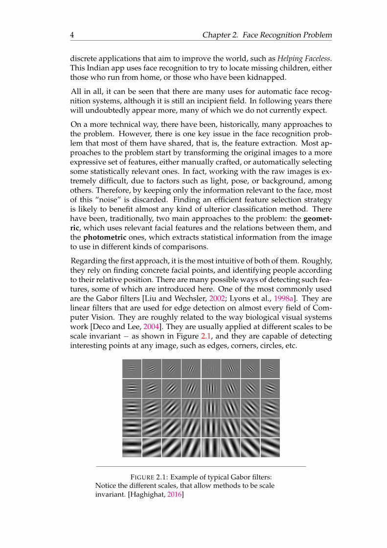
Regarding the first approach, it is the most intuitive of both of them. Roughly,they rely on finding concrete facial points, and identifying people accordingto their relative position. There are many possible ways of detecting such fea-tures, some of which are introduced here. One of the most commonly usedare the Gabor filters [Liu and Wechsler, 2002; Lyons et al., 1998a]. They arelinear filters that are used for edge detection on almost every field of Com-puter Vision. They are roughly related to the way biological visual systemswork [Deco and Lee, 2004]. They are usually applied at different scales to bescale invariant − as shown in Figure 2.1, and they are capable of detectinginteresting points at any image, such as edges, corners, circles, etc.
FIGURE 2.1: Example of typical Gabor filters:Notice the different scales, that allow methods to be scaleinvariant. [Haghighat, 2016]

Chapter 2. Face Recognition Problem 5
When applied to face recognition, they are get rid of the unnecessary elementin the image, such as sprinkles, shades or smooth color variations, keepingonly the relevant features, such as eyes, mouth, face border, etc. In practice,Gabor filters are used to locate certain elements in the face that will be laterused to identify the face [Wiskott et al., 1997]. An example of Gabor filtersapplied to face recognition can be seen in Figure 2.2. After that, it becomeseasier to find the relevant positions.
FIGURE 2.2: Example of Gabor filters in a face:Notice that only the most promiment features are kept, thusreducing image noise. [Lyons et al., 1998b]
There are many ways of using the detected facial features to perform com-parisons. Many applications look for a set of defined landmarks that canaccurately define a face. However, except in the best conditions, it is difficultto properly locate all such points. In some occasions, some of them may noteven exist in the image, Figure 2.3.
FIGURE 2.3: Occluded fiducial points
:
Even though not all fiducial points are visible, or can be easilydetected, by knowing their relative position, and using globalinformation, their position can be properly estimated. [Belhumeuret al., 2011]
In those cases, it is very common to try to fit an already existing face shapeinto the detected face, by taking the relation between their points into accountat the same time. One possible way of doing so is by using Active Shape

6 Chapter 2. Face Recognition Problem
Models. Given the set of detected landmarks, the goal is to fit them into analready defined shape. This solution is iteratively improved, until a suitablematch is found, Figure 2.4. By doing so, we can synthesize a whole faceimage into a set of defined positions, which is much easier to deal with [UtsavPrabhu and Keshav Seshadri 2009], as it provides more information.
FIGURE 2.4: Active Shape Models:Even though the starting point is far from the correct position,after some iterations the algorithm succeeds. [“An introduction toactive shape models”]
This is just an introduction, as there are many other geometric approaches,such as using Hidden Markov Models [Salah et al., 2007]. For a more
The main goal of photometric approaches is to synthesize information inimages so that only relevant information is kept, whereas all the rest is dis-carded. There are many techniques that aim to do so
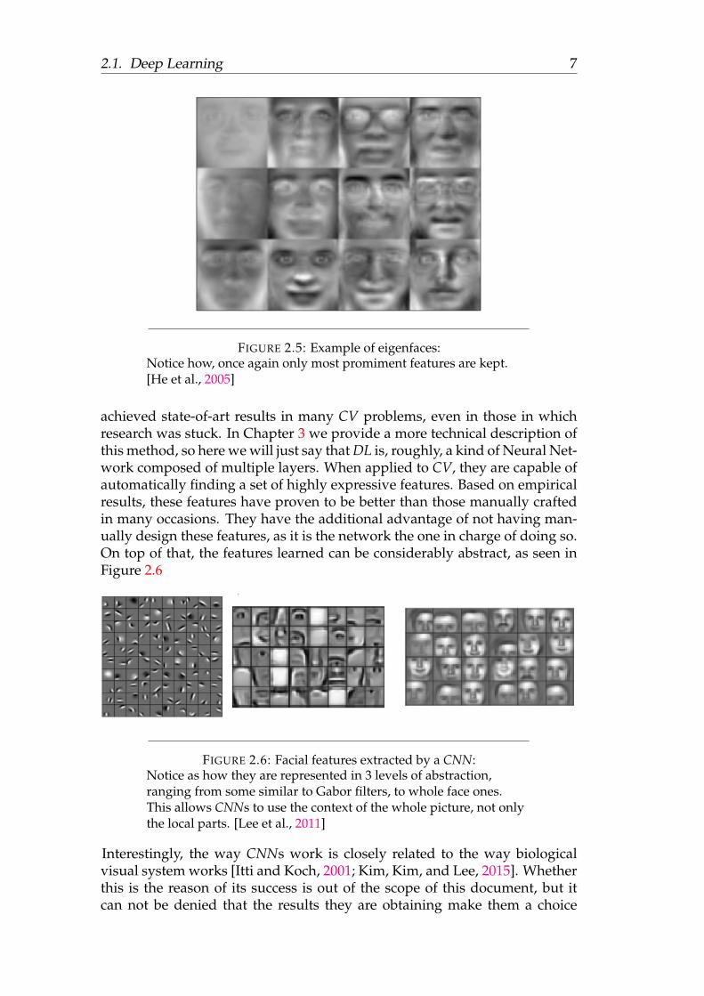
One method that has been successfully applied in this sense is the PrincipalComponent Analysis. Its main goal is to produce a set of linearly uncorrelatedfeatures from the original set. Because of this, it is often used to produce areduced representation of the data that is easier to analyze. By applying it toface images, it is capable of producing synthesized face versions called eigen-faces. Given a set of face images − high-dimensional −, eigenfaces are theeigenvectors derived from the covariance matrix of its probability distribu-tion. This provides a compact representation of faces, as it can be seen in Fig-ure 2.5. Interestingly, it has been proved that most faces can be represented asa linear combination of several eigenfaces [Turk and Pentland, 1991]. There-fore, recognition can be achieved by determining the corresponding combi-nation.
These are some of the most representative techniques, but there have beencountless more that we can not include here due to space constraints. Someof these made use of some of the introduced ones, and some others are com-pletely different. All in all, one of the main goals of all of them has been tofind a way of finding which features identify a face.
2.1 Deep Learning
In recent years a new method has appeared which has affected the wholeComputer Vision community. Since its appearance, Deep Learning, and moreconcretely Deep Neural Networks and Convolutional Neural Networks, has steadily
2.1. Deep Learning 7
FIGURE 2.5: Example of eigenfaces:Notice how, once again only most promiment features are kept.[He et al., 2005]
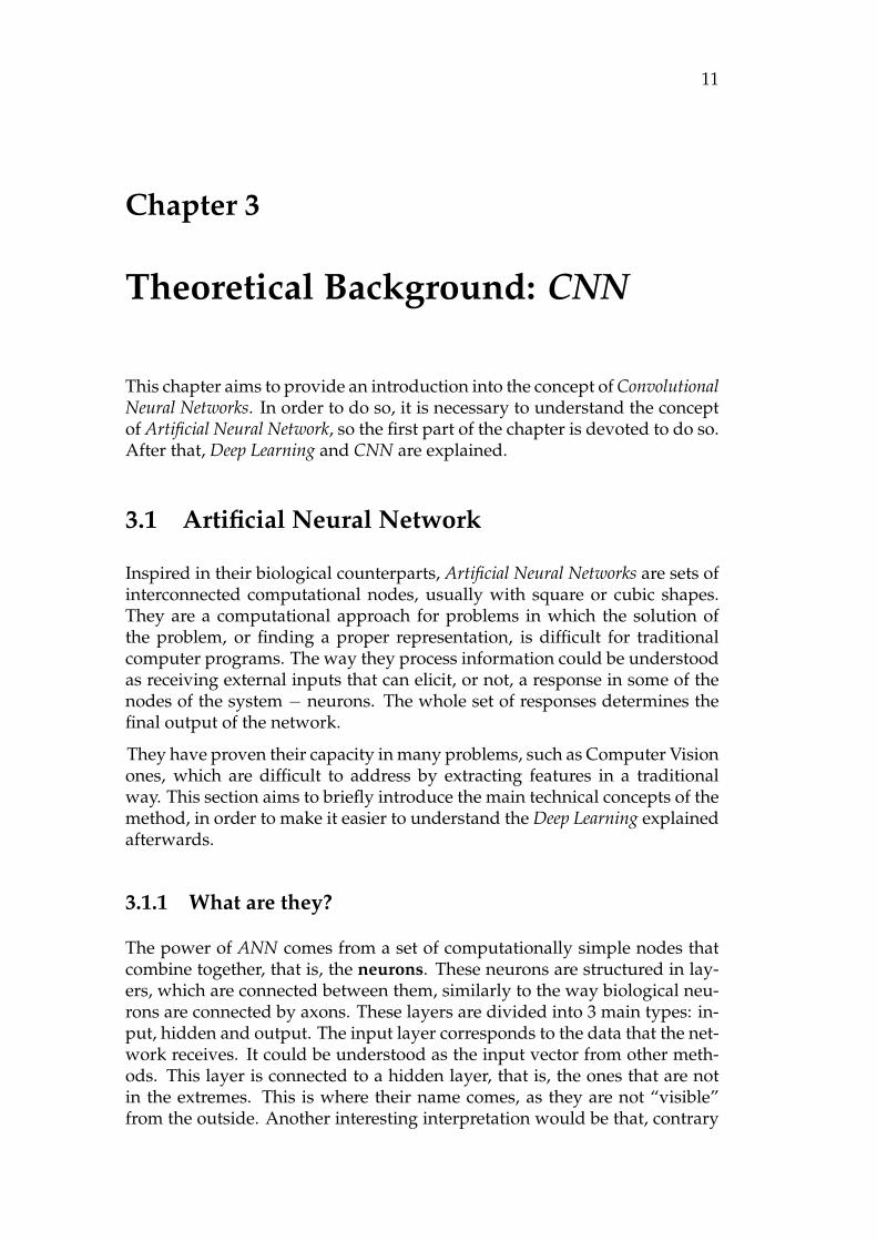
achieved state-of-art results in many CV problems, even in those in whichresearch was stuck. In Chapter 3 we provide a more technical description ofthis method, so here we will just say that DL is, roughly, a kind of Neural Net-work composed of multiple layers. When applied to CV, they are capable ofautomatically finding a set of highly expressive features. Based on empiricalresults, these features have proven to be better than those manually craftedin many occasions. They have the additional advantage of not having man-ually design these features, as it is the network the one in charge of doing so.On top of that, the features learned can be considerably abstract, as seen inFigure 2.6
FIGURE 2.6: Facial features extracted by a CNN:Notice as how they are represented in 3 levels of abstraction,ranging from some similar to Gabor filters, to whole face ones.This allows CNNs to use the context of the whole picture, not onlythe local parts. [Lee et al., 2011]
Interestingly, the way CNNs work is closely related to the way biologicalvisual system works [Itti and Koch, 2001; Kim, Kim, and Lee, 2015]. Whetherthis is the reason of its success is out of the scope of this document, but itcan not be denied that the results they are obtaining make them a choice

8 Chapter 2. Face Recognition Problem
to consider when faced with CV problems. In fact, a large number of themost successful applications of CV in recent years have used CNNs, and thistendency is expected to continue. Because of this, the work in this thesismakes use of them.
Two of the most successful applications of CNNs in the FR problem areDeepFace [Taigman et al., 2014] and FaceNet [Schroff, Kalenichenko, andPhilbin, 2015]. These two have provided state-of-art results in recent years,with the best results being obtained by the second ones. Although thereare other methods providing close results, such as involving Joint Bayesianmethods [Cao et al., 2013; Chen et al., 2013], we decided to focus on CNN.The reasons were not only result driven, but also interest driven, as we werepersonally interested in working with them.
2.2 Problems
Unfortunately, even though its potential, automatic face recognition has manyproblems. One of the most important ones is face variability in a single per-son. There are many factors that can influence so that two pictures fromthe same person look totally different, such as light, face expression or oc-clusion. Actually, when dealing with faces in controller environments, facerecognition systems are already delivering quality results, but they still haveproblems when faced with faces in the “wild”. Even more, factors such assunglasses, beards, different hairstyles, or even age, can greatly difficult thetask. An example of these problems can be seen in Figure 2.7.
Another problem to be taken into account is the environment. Except incontrolled scenarios, face pictures have very different backgrounds, whichcan make the problem of face recognition more difficult. In order to addressthis issue, many of the most successful systems focus on treating the facealone, discarding all the surroundings.
Taking all of it into consideration, our goal was to develop a system capableof working with faces in uncontrolled environments. In order to do so, weused Convolutional Neural Networks as a feature extraction method. We alsoplanned on applying some pre-processing in order to minimizing the impactof the environment, and make our system more robust. That being said, wewere aware of the difficulties involved in such a project, so we were cautiousabout the expected results.

2.2. Problems 9
FIGURE 2.7: Variability in a face:Even though they all belong to the same person, they are hardlyrecognized as such, even by a human.

11
Chapter 3
Theoretical Background: CNN
This chapter aims to provide an introduction into the concept of ConvolutionalNeural Networks. In order to do so, it is necessary to understand the conceptof Artificial Neural Network, so the first part of the chapter is devoted to do so.After that, Deep Learning and CNN are explained.
3.1 Artificial Neural Network
Inspired in their biological counterparts, Artificial Neural Networks are sets ofinterconnected computational nodes, usually with square or cubic shapes.They are a computational approach for problems in which the solution ofthe problem, or finding a proper representation, is difficult for traditionalcomputer programs. The way they process information could be understoodas receiving external inputs that can elicit, or not, a response in some of thenodes of the system − neurons. The whole set of responses determines thefinal output of the network.
They have proven their capacity in many problems, such as Computer Visionones, which are difficult to address by extracting features in a traditionalway. This section aims to briefly introduce the main technical concepts of themethod, in order to make it easier to understand the Deep Learning explainedafterwards.
3.1.1 What are they?
The power of ANN comes from a set of computationally simple nodes thatcombine together, that is, the neurons. These neurons are structured in lay-ers, which are connected between them, similarly to the way biological neu-rons are connected by axons. These layers are divided into 3 main types: in-put, hidden and output. The input layer corresponds to the data that the net-work receives. It could be understood as the input vector from other meth-ods. This layer is connected to a hidden layer, that is, the ones that are notin the extremes. This is where their name comes, as they are not “visible”from the outside. Another interesting interpretation would be that, contrary
12 Chapter 3. Theoretical Background: CNN
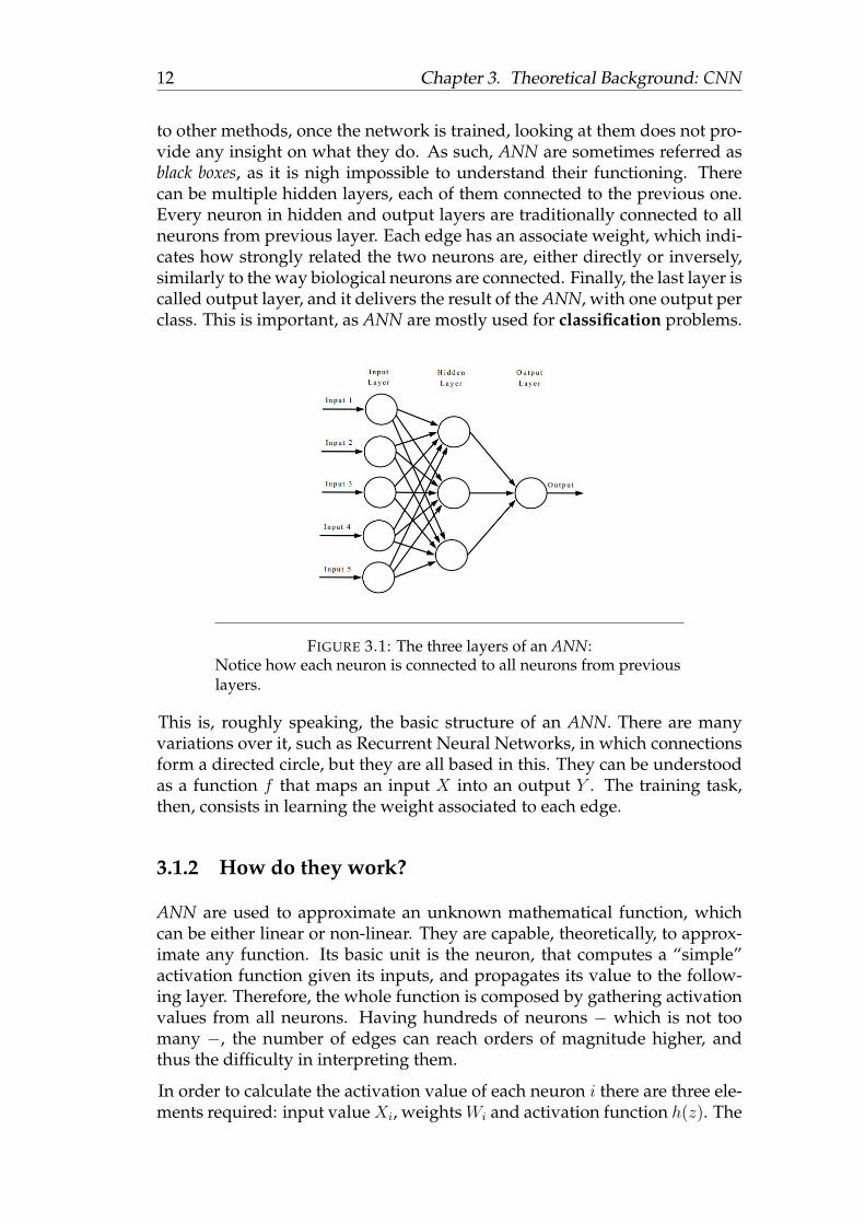
to other methods, once the network is trained, looking at them does not pro-vide any insight on what they do. As such, ANN are sometimes referred asblack boxes, as it is nigh impossible to understand their functioning. Therecan be multiple hidden layers, each of them connected to the previous one.Every neuron in hidden and output layers are traditionally connected to allneurons from previous layer. Each edge has an associate weight, which indi-cates how strongly related the two neurons are, either directly or inversely,similarly to the way biological neurons are connected. Finally, the last layer iscalled output layer, and it delivers the result of the ANN, with one output perclass. This is important, as ANN are mostly used for classification problems.
FIGURE 3.1: The three layers of an ANN:Notice how each neuron is connected to all neurons from previouslayers.
This is, roughly speaking, the basic structure of an ANN. There are manyvariations over it, such as Recurrent Neural Networks, in which connectionsform a directed circle, but they are all based in this. They can be understoodas a function f that maps an input X into an output Y . The training task,then, consists in learning the weight associated to each edge.
3.1.2 How do they work?
ANN are used to approximate an unknown mathematical function, whichcan be either linear or non-linear. They are capable, theoretically, to approx-imate any function. Its basic unit is the neuron, that computes a “simple”activation function given its inputs, and propagates its value to the follow-ing layer. Therefore, the whole function is composed by gathering activationvalues from all neurons. Having hundreds of neurons − which is not toomany −, the number of edges can reach orders of magnitude higher, andthus the difficulty in interpreting them.
In order to calculate the activation value of each neuron i there are three ele-ments required: input valueXi, weightsWi and activation function h(z). The
3.1. Artificial Neural Network 13
input value are the outputs from previous layer that the neuron receives. Asalready stated, each neuron is most often connected to all neurons from pre-vious layers. Additionally, a bias value b is usually passed to each layer, notcoming from any neuron. As each edge connecting two neurons has its ownweight, the value used by neuron i from layer l to calculate the activationfunction, given N inputs, can be expressed as:
yi = h(xl−1) =N∑j
(Wi,j × xl−1,j) + bl (3.1)
, representing a linear addition of all of them. The activation function φ is anon linear function representing the degree of activation of the neuron, andit can be defined as:
f(x) = φ(h(x)) (3.2)
There are many possibilities depending on the problem at hand, such as thehyperbolic tangent:
φ(x) =e2x − 1
e2x + 1(3.3)
, or the logistic function:
φ(x) =1
1 + e−x(3.4)
.
All these have in common that they usually have a range between 0 and 1,or -1 and 1. There is no definite answer regarding which to choose, but thereare some properties that they should fulfill, such as being continuously differ-entiable. If activation functions such as Equation 3.5 were used, the networkwould be impossible to train1. In the end, the idea behind them is that theyhave to produce a smooth transformation given the input values. In otherwords, a small change in input produces a small change in output.
φ(x) =
1 if x >= 00 if x < 0
(3.5)
.
For two neural layers, the output of the last one can be interpreted as a com-position of functions, that is, the activation function of the first and the onefrom the second. This allows expressing complex non-linear functions with-out explicitly coding them, just by the power of many small computations.
1The reason is that the gradient would be zero, so gradient-based methods could notlearn. This is further explained in Section 3.2
14 Chapter 3. Theoretical Background: CNN
All in all, when specifying a neural network the main decisions are the ar-chitecture, that is, number of layers and neurons in each of them, and theactivation function. Once this is set, the only part missing is to choose thetraining strategy.
3.2 How are they trained
One of the main requirements for training this kind of algorithms is data.All learning algorithms use data in their training processes, but ANN requiremore than most. As it will be explained in following chapters, this became areal issue during the project.
Given the data, there are various learning algorithms, from which gradientdescent combined with backpropagation can be considered, given its widelyspread use, the most successful of all of them. In fact, to a certain degree itcould be considered that using it is enough for training most ANNs.
This algorithm starts by initializing all weights in the network, which can bedone following various strategies. Some of the most common ones includedrawing them from a probability distribution, or randomly setting them, al-though low values are advisable. The process followed afterwards consists of3 phases that are repeated many times over. In the first one, an input instanceis propagated through all the network, and the output values are calculated.Then, this output is evaluated, using a loss function, with the correct output,and this is used to calculate how far off the network is. The final phase con-sists in updating each weight in order to minimize the obtained error. This isdone by obtaining the gradient of each neuron, that could be understood as a“step” towards to actual value. When these three phases are repeated for allinput instances we consider this an epoch. The algorithm can run for as manyepochs as specified, or as required to find the solution.
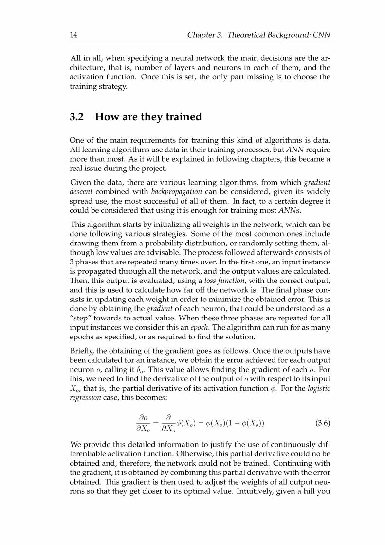
Briefly, the obtaining of the gradient goes as follows. Once the outputs havebeen calculated for an instance, we obtain the error achieved for each outputneuron o, calling it δo. This value allows finding the gradient of each o. Forthis, we need to find the derivative of the output of o with respect to its inputXo, that is, the partial derivative of its activation function φ. For the logisticregression case, this becomes:
∂o
∂Xo
=∂
∂Xo
φ(Xo) = φ(Xo)(1− φ(Xo)) (3.6)
We provide this detailed information to justify the use of continuously dif-ferentiable activation function. Otherwise, this partial derivative could no beobtained and, therefore, the network could not be trained. Continuing withthe gradient, it is obtained by combining this partial derivative with the errorobtained. This gradient is then used to adjust the weights of all output neu-rons so that they get closer to its optimal value. Intuitively, given a hill you

3.3. Deep Learning 15
are descending, the gradient would be an step in the direction with an steep-est descent, that brings you closer to the floor. After adjusting the weights forthe output layers, the same process needs to be done for the remaining lay-ers, except for the input one. In order to do so, each layers needs the δ of thenext layer to be calculated. This is the reason by it is called backpropagation,because it starts in the output layer, and from there it goes backward. In theend, all the edge weights have been updated, and thus a new instance can beprocessed.
There are two main ways of applying backpropagation that need to be men-tioned, stochastic and batch. The stochastic approach is the one presented,in which weights are updated after each instance. This introduces a certainamount of randomness, preventing the algorithm from getting stuck in localoptima. The other approach, instead, applies the weight update only afterhaving processed a set of instances, using the average error. This usuallyleads makes the algorithm converge faster to a local minima, which may ac-tually be a good result. A compromise between them both can be achievedusing the mini-batch strategy. This one uses small batches with randomlyselected samples, which combines both strategies benefits.
Therefore, it can be concluded that the learning task for neural networksconsists in finding the right weights. The algorithm explained here is theone most commonly used, although many other architectures use some vari-ations over this basic algorithm.
There are also other ways of learning the weights, such as genetic algo-rithms [Montana and Davis, 1989] or simulated annealing [Aarts and Korst,1989; Yamazaki, Souto, and Ludermir, 2002]. However, with some interestingexceptions, these methods are rarely used, being backpropagation the mostcommonly used algorithm by far. The choice of the algorithm will affect theperformance of the whole method, so it is an important issue to take intoaccount.
We have provided a description of the, arguably, most commonly used ANN,that is, the Multi Layer Perceptron. Variations over it lead to other well knowntypes such as Recurrent Neural Networks (RNN) or Radial Basis Function net-work (RBF).
3.3 Deep Learning
One of the key aspects in most machine learning methods is the way datais represented, that is, which features to use. If the features used are badlychosen, the method will fail regardless of its quality. Even more, this selectionaffects the knowledge with which the method can work: if you have trainedyour market analysis algorithm with numerical values, it will not be able tomake any sense from a written report, no matter its quality. Therefore, it is nosurprise that there has been an historical interest on finding the appropriate
16 Chapter 3. Theoretical Background: CNN
features. This becomes especially relevant in the case of Computer Visionproblems. The reason is that, when faced with an image, there are usuallyway too many features − a simple 640× 480 RGB image has almost 1 millionpixels −, and most of them are irrelevant. Because of this, it is important tofind some way of condensing this information in a more compact way.
There are two main ways of obtaining features, manually choosing them− such as physiological values in medical applications − or automaticallygenerating them, an approach known as representation learning. The lat-ter has proven to be more effective in problems such as computer vision,as it is very difficult for us humans to know what makes an image distin-guishable. Instead, in many cases machines have been able to determinewhich features were relevant for them, resulting in some state of art results.The most paradigmatic case of representation learning are the autoencoders.They perform a 2 step process, first they encode the information they receiveinto a compressed representation, and they later try to decode, or reconstruct,the original input from this reduced representation.
We are going to focus on Computer Vision problems from now on, as it willmake it easier to understand some of the next sections. Regarding the fea-tures extracted, people may have some clear ideas about what makes an ob-ject, such as a car, recognizable. Having 4 wheels, doors in the lateral, aglass at the front, it is made of metal, etc. However, these are high level fea-tures, that are not easy for a machine to find in an image. To make it evenworse, each kind of object in the world has its particular features, usuallywith a large intra-class variability. Because of this, developing a general ob-ject recognition application would be impossible, as we would need manu-ally selected features for each of them. Therefore, it has not been a successfulline of research recently. On the contrary, if machines are capable of deter-mining on their own what is representative of an object for them on theirown, they will have the potential of learning how to represent any objectthey are trained with.
However, there is an additional difficulty for this kind of problems, that is,the variability depending on the conditions of each picture. We do not onlyhave to deal with the intra-class variability, but also the same object variabil-ity. The same car can be pictured in almost endless ways, depending on thepose of the car, light conditions, image quality, etc. Us humans are capableof making rid of this variation by extracting what we could consider abstractfeatures. These features can be include the ones we mentioned before, suchas number of wheels, but also others we are not aware of, such as the factthat they are usually on a road, or that their wheels should be in contact withthe floor. In order to develop a successful representation learning method, itshould be able to extract this kind of high-level features, regardless of theirvariation. The problem is that this process can be extremely difficult to de-velop into a machine, which may lead into thinking that it makes no senseto make the effort of doing so. This is, precisely, where Deep Learning hasproven to be extremely useful.
3.3. Deep Learning 17
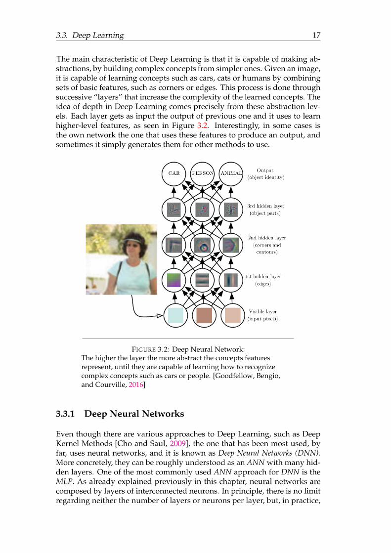
The main characteristic of Deep Learning is that it is capable of making ab-stractions, by building complex concepts from simpler ones. Given an image,it is capable of learning concepts such as cars, cats or humans by combiningsets of basic features, such as corners or edges. This process is done throughsuccessive “layers” that increase the complexity of the learned concepts. Theidea of depth in Deep Learning comes precisely from these abstraction lev-els. Each layer gets as input the output of previous one and it uses to learnhigher-level features, as seen in Figure 3.2. Interestingly, in some cases isthe own network the one that uses these features to produce an output, andsometimes it simply generates them for other methods to use.
FIGURE 3.2: Deep Neural Network:The higher the layer the more abstract the concepts featuresrepresent, until they are capable of learning how to recognizecomplex concepts such as cars or people. [Goodfellow, Bengio,and Courville, 2016]
3.3.1 Deep Neural Networks
Even though there are various approaches to Deep Learning, such as DeepKernel Methods [Cho and Saul, 2009], the one that has been most used, byfar, uses neural networks, and it is known as Deep Neural Networks (DNN).More concretely, they can be roughly understood as an ANN with many hid-den layers. One of the most commonly used ANN approach for DNN is theMLP. As already explained previously in this chapter, neural networks arecomposed by layers of interconnected neurons. In principle, there is no limitregarding neither the number of layers or neurons per layer, but, in practice,
18 Chapter 3. Theoretical Background: CNN
it has been almost impossible to successfully training more than a handfulof hidden layers. As already explained, the number of weights in a networkcan easily reach the thousands, or even millions in the larger ones, meaninga large number of parameters to learn. This requires both extremely largecomputational times and data to feed to the training stages. There have beenattempts at doing so since decades ago, but it has not been until the late 2000sthat the means for effectively doing so have been available.
There are various factors that allowed to train this kind of networks. Thefirst of all is the increase in computational power that computers have experi-enced. Not only today’s computers are much more powerful than those froma decade ago, but also the appearance of graphical cards has greatly boostedthe speed of those methods. Graphics Processing Units, or GPU’s, werefirstly designed to allow computers run demanding graphical programs, mainlyvideogames. In order to do so, they excelled at rapidly performing largeamounts of simple operations, as rendering methods needed. Seeing this, itbecame apparent that they could be used for other kind of applications withsimilar needs, such as, precisely, DNN. Nowadays, most DNN researchersand users use GPUs to run theirs, as they can reduce the running time in or-ders of magnitude. This has popularized the use of DNN, as it is no longernecessary to use expensive super-computers in order to train networks in areasonable amount of time.
The other factor that helped at DNN training was the new data oriented cul-ture that arose in the decade of 2000s. As data mining and machine learningmade it possible to analyze all kinds of data in a fast and reliable way, manyentities wanted to make use of it. In order to do so, they started gatheringlarge amounts of data, and converting them into usable datasets. These covera great range of disciplines, such as health, economics, social behavior, etc.Although some of these datasets were of private use, many of them were re-leased to the public. It became a self-feeding circle, because as more data wasavailable to study, the better the analyzing techniques became, which luredmore people into using it. This allowed the creation of large datasets, withmillions of instances, that could be used to train ANN with great numbers ofparameters to learn, without overfitting2.
The final factor that allowed the popularization of DNN was the appearanceof new methods of training them. Although the two previous facts helped,without advanced training algorithms we could not have made use of them.It is commonly considered that it was Hinton who established the basis formodern Deep Learning in 2006 [Hinton, Osindero, and Teh, 2006]. In thatpublication he proposed a way of training deep neural networks in a fast andsuccessful way. This was achieved by treating each layer as a Restricted Botz-mann machine, and training them one at a time, thus pre-training the net-work weights. After that, the network was fine-tuned as a whole. This break-through allowed to train multiple layered − deep − networks that could not
2Overfitting means that a learning method has tried to model the training set too much,and, as a result, it does not generalize well to new data. It is a common issue on DNN

3.3. Deep Learning 19
have been trained previously, as they would have ended up overfitting. Af-ter that, many other methods have been developed in order to train deepnetworks, such as ReLU layers or dropout regularization.
3.3.2 Convolutional Neural Networks
Among the Deep Neural Networks, the ones that are most widely used inComputer Vision problems are the Convolutional Neural Networks, based inthe Multi Layer Perceptron architecture. Whereas normal ANNs are inspiredin general neuronal behavior, CNNs follow the same principles as animalsvisual cortex. This consists in neurons that process only small portions ofthe input image − or visual field − and are in charge of recognizing relevantpatterns. These neurons are stacked in structures similar to layers, allowingincreasingly complex patterns. On its own, this may remind of the generalDNN structure. However, there is a key issue differentiating them, that is,shared weights.
As already explained previously in this section, the number of weights tolearn for any image is outstandingly large. This is usually impossible to ad-dress if faced as a normal MLP. Even worse, this full connectivity betweensuccessive layers is, in some cases, unnecessary, as spatial position is notconsidered. CNNs, on the other hand, focus only on local correlation, i.e.each neuron only considers a small section of its input as a whole, and disre-gards the rest, thus saving a lot of edges and taking into account the relationbetween close pixels. On top of that, recognizable elements are the same re-gardless of their position in the image, p.e. it makes sense to look for edgesand corners around all the image. Therefore, each neuron will look for thesame features than the rest of neurons in its layer, but in different locations.As such, the shared weights concept they use consists in that there is only asingle set of weights for all neurons in a layer. The part of the input space towhich a neuron is connected is called receptive field, and it can overlap withthe one from other neurons. Each receptive field is a 3D space with widthand height of the same, and the number of input channels. Therefore, foreach layer there is only one weight per value in the receptive field. As such,if the receptive field is 5 × 5 × 3, there will be only 75 weights in that layer,used by all of its neurons. This makes it possible to train large networks, asthe number of weights remains comparatively small. That being said, notall the layers in CNNs follow these rules. Instead, this type of layer is calledConvolutional Layer, but there are other ones that will be explained further inthis section. However, the use of Convolutional Layers allow greatly reduc-ing the number of weights in the network, and are the most iconic ones fromCNNs. The set of weights of each layer is called the kernel, or filter, of thatlayer. The reason is that, when they are shared, a forward pass of the layercan be interpreted as the convolution of weights and the input. The mostcommonly used activation function is the Rectifier Linear Unit (ReLu), whichapplies the following function to the output of the neuron: f(x) = max(0, x).Variations over this function are also used, such as the Noisy ReLu
20 Chapter 3. Theoretical Background: CNN
The neuron layers are stacked, and so their outputs form 3D volumes. The in-put of the first layer, that is, the image itself, can also be considered such a 3Dvolume: width× height× channels. Each stack of layers use a different kernelconfiguration, and all the layers in it are connected to all layers in previousstack. The main parameters to take into account in CNN layers are:
• Kernel size: the width and height of the receptive field for the neuronsin that stack. Both sides are usually of equal size − square kernels.
• Stride: Each neuron processes a region of the input space. As theseregions can overlap, the stride indicates the distance between their cen-ters. As such, a stride of 1 means that each neuron processes the sameregion as their neighbor except for one column. The larger the stridethe smaller the output width and height of that layer.
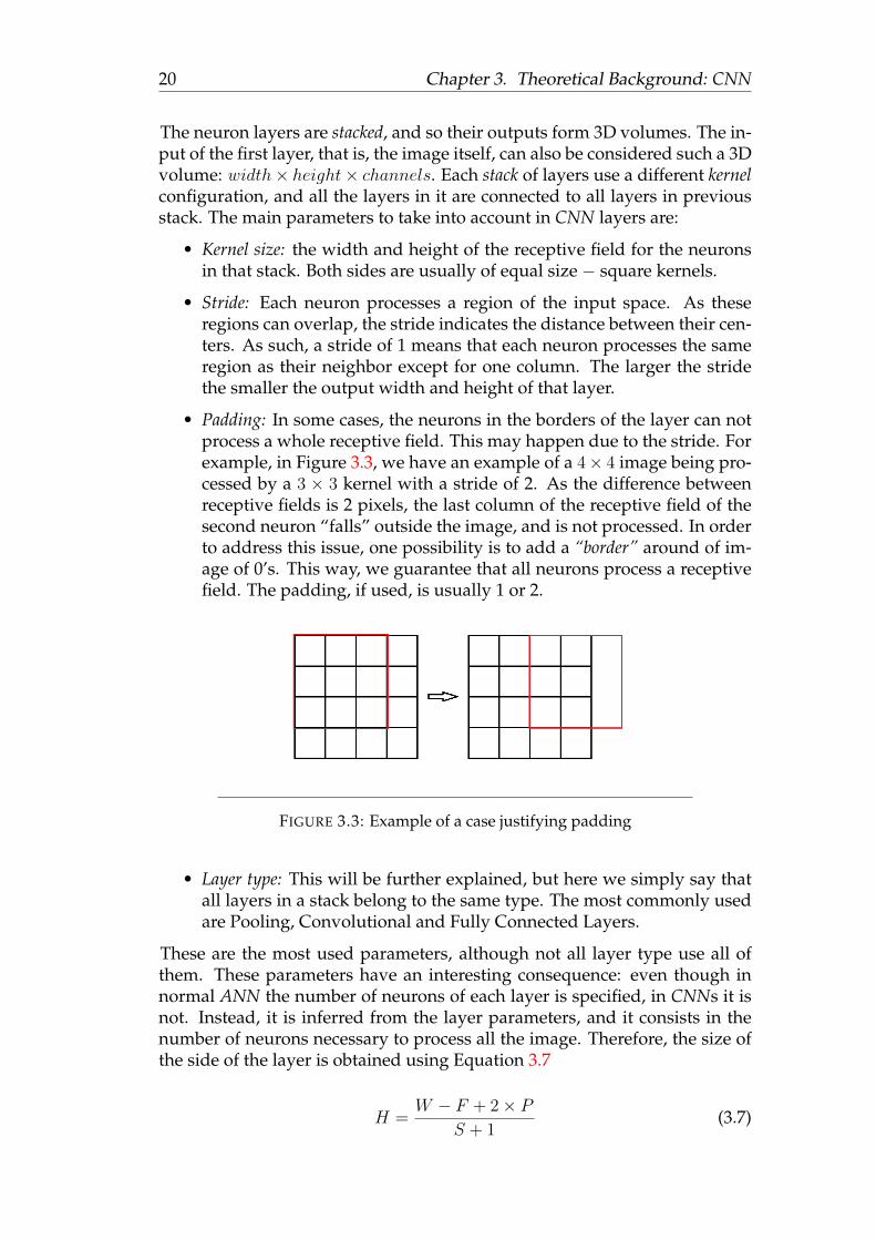
• Padding: In some cases, the neurons in the borders of the layer can notprocess a whole receptive field. This may happen due to the stride. Forexample, in Figure 3.3, we have an example of a 4× 4 image being pro-cessed by a 3 × 3 kernel with a stride of 2. As the difference betweenreceptive fields is 2 pixels, the last column of the receptive field of thesecond neuron “falls” outside the image, and is not processed. In orderto address this issue, one possibility is to add a “border” around of im-age of 0’s. This way, we guarantee that all neurons process a receptivefield. The padding, if used, is usually 1 or 2.
FIGURE 3.3: Example of a case justifying padding
• Layer type: This will be further explained, but here we simply say thatall layers in a stack belong to the same type. The most commonly usedare Pooling, Convolutional and Fully Connected Layers.
These are the most used parameters, although not all layer type use all ofthem. These parameters have an interesting consequence: even though innormal ANN the number of neurons of each layer is specified, in CNNs it isnot. Instead, it is inferred from the layer parameters, and it consists in thenumber of neurons necessary to process all the image. Therefore, the size ofthe side of the layer is obtained using Equation 3.7
H =W − F + 2× P
S + 1(3.7)

3.3. Deep Learning 21
, where W is the side of the input space, F the side of the kernel used, Pcorresponds to the padding, and S to the string. Therefore, the output of alllayers in a stack will be the same. This, together with the number of layersstacked indicate the size of the output of that stack. That being said, theoutput of a layer will never be larger in width and height than its input,and most often it will be smaller. The stride parameter, especially, has thepotential of performing large reductions, as a stride of 2 will halve the imageside size. Therefore, as the image is further propagated through the networkit gets smaller (Figure 3.4). This means that each neuron of the last layers willprocess larger patches from the original image.
FIGURE 3.4: Example of a cnnHere we can see each stack of layers, having 6, 6, 16 layers eachand so on. It also shows how each neuron only processes a patchof its input. The image size keeps reducing until reaching the FullyConnected Layers. [Pham, 2012]
Even though the differences with normal MLPs, the way they are trained isbasically the same, by using gradient descent with backpropagation, and itsgoal is the learn each layers weights.
Layer types
In this section we introduce the 4 most used layer types, together with a fifthnot so common, but relevant for our project.
• Convolutional Layer: The most iconic layer has already been introduced.It is inspired in traditional MLPs, but having some major differences.The main ones are that each layer has a single set of weights for all neu-rons − shared weights −, and that each neuron only processes a smallpart of the input space. It uses all the parameters introduced in previ-ous section.
• Pooling Layer: It is common to include these layers between successivestacks of convolutional ones, in order to progressively reduce the size ofthe image representation. It works by taking each channel of its recep-tive field, and resizes it by keeping only the maximum of its values. Itis usually used with 2 × 2 kernels, and a stride of 2, which halves eachside size. This reduces the overall size in 75% by picking the largest

22 Chapter 3. Theoretical Background: CNN
of 2 × 2 patches. This kind of layers does not have weights that needtraining, and it only uses the stride and kernel size parameters. Its util-ity consists in reducing the amount of weights to learn, which reducescomputational time as well as probability of overfitting.
• Fully Connected Layer: These layers are basically neural layers connectedto all neurons from previous layer, as the ones from regular ANNs. Inthis case, they do not use any of the introduced parameters, using in-stead the number of neurons. The output they produce could be under-stood as a compact feature vector representing the input image. Theyare also used as output layers, with one neuron per output, as usual.
• Locally Connected Layer: The last presented layer is really similar to theConvolutional Layer, but it does not use the shared weight strategy. Thisstrategy is justified in normal Convolutional Layers because the rele-vant features are usually independent of their position in the image.However, there are cases in which this may not hold true. If you know,for example, that all your images will have a face centered to the sameposition, it makes sense to look for different features at the eye zonethan at the mouth zone. This is achieved by giving each neuron its ownset of weights, similarly to regular ANN, but they still only process theirreceptive field. These layers are commonly used after some Convolu-tional and Pooling ones due to 2 reasons. The first one is that, in orderfor the features from, p.e, eyes and mouth, to be different, they needto be a relatively abstract ones. Basic structures, such as edges or cor-ners, are relevant in both cases. As already explained, this abstractionlevel is achieved by applying successive neuron layers, which builds“complex” features by means of simpler ones. Thus, the utility of usingsome Convolutional Layers before. The other reason is that using Lo-cally Connected Layers introduces a large amount of weights into thenetwork, making it more prone to overfitting. Then, it is better to usethem when the image has already been reduced by previous layers. Allin all, this type of layer is not very commonly used due to it requir-ing a fixed spatial distribution. However, if this condition is fulfilled,and you have enough data to prevent overfitting, they are an excellentchoice.
There are other considerations to take into account when dealing with CNNs,such as using Dropout − a regularization method that randomly disablesneurons to prevent overfitting −, but we deem the provided informationenough for the purpose of this document.
23
Chapter 4
My Proposal
When I had to face the problem, my first step was to research the history andcurrent state of the field, as explained in Chapter 2. This gave me a goodbasis on what I could expect, which methods I could use, and which ones Icould discard. First of all I briefly considered using a geometric approach, byusing some of the existing software in order to detect relevant facial features,and later use them as features in a classificator. This appealed to me due toits intuitiveness: the process could be easily understood, regardless the spe-cific mathematical details. However, the existing research lead me, quite pre-dictably, to the field of CNNs. As already explained, they are providing newresult benchmarks in many Computer Vision applications, including FaceRecognition. Additionally, due to the interest in the field, there is a largeamount of research in it. Even more, even though some of this research be-longs to companies and it is therefore private, there are many papers that arepublicly available. These two factors − quality of the results and availabil-ity of information − lead us to choose to use CNNs in our Face Recognitionsystem.
At this point we faced a decision, that is, whether to design the system onour own, or to make use of some of the already existing ones to guide us.Each one of them had its pros and cons. If we started from zero, we couldclaim all of its credit, even more if it produced quality result. Additionally,at a personal level we could feel more rewarded, which could somewhatmotivate us to continue. On the other hand, there were two main drawbacks.The first one was that we could not guarantee that we would succeed, whichwould make all of our work useless. Moreover, in order to succeed we wouldlikely require to test lots of CNN configurations, which pose a large problem.One of the main problems of CNNs is that they require both lots of data andlarge computational time. In other machine learning methods, it is a commonpractice to make a protoype of the system and test it in small pieces of data.Once the system is approximately configured, tests with the final datasetscan start and, by that moment, there has been plenty of time to gather it.However, due to CNNs data requirements this was not possible, as testingwith little data would be meaningless, as we would not achieve any kindof result. Therefore, we could only start the testing after we had gatheredthe required data. This would leave us with little time for testing and, asalready explained, time is exactly what CNNs require. This would mean that

24 Chapter 4. My Proposal
FIGURE 4.1: FaceNet performing in poor light conditions[Schroff, Kalenichenko, and Philbin, 2015]
we would not have time to properly test many CNN configurations, and,therefore, we would be unlikely to succeed. This is why we decided to baseour system in some of the already existing methods. Even though this wouldmean that we could claim less of the resulting work, we would have a muchhigher chance to succeed, and we could make more thorough tests. In orderto determine which paper to choose, we gathered some of the state of artresearches that were publicly described.
From all the papers and methods we considered, we ended up selecting twoof the most interesting ones. The first one was FaceNet [Schroff, Kalenichenko,and Philbin, 2015], developed as part of Google’s AI research. In the lastdecades, Google has made huge investments on expanding its AI capabili-ties. One of its most well known examples is the DeepMind company [Deep-Mind, 2016]. Due to the company’s vast resources, it has obtained some ofthe current state-of-art AI systems. In the FaceNet case, its results are amongthe best ones worldwide. In fact, even though it does perform extremelywell− almost perfectly− in benchmark datasets (Section 5.4.1), this is not itsmain feature. Instead, it is developed taking into account much more difficultsituations that the ones in such datasets, as seen in Figure 4.1.
This system, which uses Deep Learning, has been trained using a massive200 million instances private dataset. They must be credited with being ableof making use of that much data in such a successful way. Given the qualityof the results, the robustness of the method and the fact that they provide
4.1. What did we do? 25
a description on how they implemented it, we considered that it would beinteresting to inspire our work in it.
For the other option, we also considered one of the other technological leadercompanies, in this case, Facebook. Maybe more well known by the averageuser, their face recognition capabilities can be found on a daily basis whenusing their website. As such, it can be easily checked that it performs sur-prisingly well. The face recognition method they developed, called Deep-Face [Taigman et al., 2014], is also publicly available. Even though the re-sults in some of the most well known benchmark datasets are not as goodas FaceNet’s, they were close to them nevertheless. The fact that they haveit working in the most used social network is further proof of its capabili-ties. On top of that, the description of the method was extremely straight-forward, which made it easy to comprehend and implement. Finally, thetraining dataset consisted of roughly 4.4 million images, from an also privatedataset.
In the end we decided to use DeepFace. In order to make this choice wetook different factors into account, such as feasibility or implementing themor quality of description. We discarded FaceNet due to technical reasons: wewere unable to even remotely match the quality of their dataset, having morethan 200 million images. Because of this, we considered that, even thoughtheir method was good, given the obtained results, we could not achievethem due to a lack of data. On the other hand, DeepFace provided a good bal-ance, as it achieved good results and the method was thoroughly explainedin their paper. Although their dataset was large, it was much smaller thanFaceNet’s. We expected to gather enough data so that, even though we maynot reach their results, we could get close enough. On top of that, the wayit was developed allowed for a direct way of addressing the face recognitionproblem.
4.1 What did we do?
Making use of DeepFace guidelines, we have developed a system capable ofperforming face recognition among a set of stored faces. New people can beintroduced into the system both automatically and manually, which makesit suitable for different scenarios. On top of that, it can work with videos, byidentifying the people who appear there, and surround them with the facebounding box. The system is composed of two main parts: the extraction offeatures by means of a CNN, and using these features to identify a person. Inthis section we provide an in-depth explanation of how each of them works,as well as the explanation of how the video analysis works, and an onlineweb tool we developed.
26 Chapter 4. My Proposal
4.1.1 Feature extraction
The first part of the system consists in automatically extracting relevant fea-tures from the image. These features will later be used to determine whethertwo images belong or not to the same person. As such, it is extremely impor-tant for it to work properly. In this sense, we have used the implementationproposed in [Taigman et al., 2014]. They used a two step process in order todo so: first, they frontalized the face so that they all looked at front, followedby a CNN configuration that made use of that.
The intuition behind is that face recognition is difficult to address due to thelarge variability between face poses. If the CNN received the images as theyare, it would have to deal with people looking in all directions, backgroundnoise, different positions of the face in the image, etc. Therefore, it makessense to first try to reduce this variability by centering faces in the image
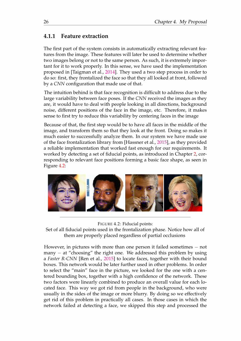
Because of that, the first step would be to have all faces in the middle of theimage, and transform them so that they look at the front. Doing so makes itmuch easier to successfully analyze them. In our system we have made useof the face frontalization library from [Hassner et al., 2015], as they provideda reliable implementation that worked fast enough for our requirements. Itworked by detecting a set of fiducial points, as introduced in Chapter 2, cor-responding to relevant face positions forming a basic face shape, as seen inFigure 4.2:
FIGURE 4.2: Fiducial points:Set of all fiducial points used in the frontalization phase. Notice how all of
them are properly placed regardless of partial occlusions
However, in pictures with more than one person it failed sometimes − notmany − at “choosing” the right one. We addressed this problem by usinga Faster R-CNN [Ren et al., 2015] to locate faces, together with their boundboxes. This network would be later further used in other problems. In orderto select the “main” face in the picture, we looked for the one with a cen-tered bounding box, together with a high confidence of the network. Thesetwo factors were linearly combined to produce an overall value for each lo-cated face. This way we got rid from people in the background, who wereusually in the sides of the image or more blurry. By doing so we effectivelyget rid of this problem in practically all cases. In those cases in which thenetwork failed at detecting a face, we skipped this step and processed the

4.1. What did we do? 27
image directly. Even though we risked to fail at choosing the proper face, weacceptable. Anyway, we expert to address this issue in the future.
After using the library on face images, we produced 140 × 140 RGB images,which an oval in the middle with the frontalized face, and the remainingspace black. In Figure 4.3 we provide some examples of the results we haveobtained using it. There are examples of both successful frontalizations aswell as unsuccessful ones, but we had to find a way of automatically decidingwhich group each image belonged to.
FIGURE 4.3: Examples of frontalized faces:In the first two columns there are examples of properly frontalizedones, whereas in the last two there are cases in whichfrontalization has not worked properly.
In order to detect whether the image had been properly frontalized, we hadto take two cases into account, that is, the ones in which no face was detected,and the ones in which frontalization failed. In the first case we had difficultfaces, such as ones involving glasses, weird face expressions and so on, inwhich the frontalization library failed to detect the fiducial points. In thesecases the image was not frontalized, but we resized them to 140×140, so thatthey could still be used. This was not a direct transformation, as it wouldhave distorted the image. Instead, set the longest side to 140 and the shortestone was modified to keep the proportion, and the remaining space in themargins was filled in black.
At first we decided to use them too, both in training and testing, hoping thatthe CNN would be able to disregard the background on its own. However,empirical evidence from the testing showed that the CNN was unable to doso, and it failed most of the times. Therefore, in the end we decided to discard

28 Chapter 4. My Proposal
these images−which, in fact, accounted for a small percentage of the total−both in testing and training.
The second problematic case were those images that were erroneously frontal-ized, such as the ones in Figure 4.3. This problem proved to be a rather diffi-cult one, as, contrary to the previous case, the program was unable to knowwhether it had succeeded or not. Therefore, once we whole dataset was pro-cessed, we had to perform a cleaning of the images, in which we tried todiscards as many of such images as possible. This was done in two phases.In the first one, we used the aforementioned Faster R-CNN in order to detectfaces in the image. As some failed frontalizations resulted in “impossible”faces, they would not be detected. Those images would be, therefore, dis-carded. In the second step, we used a geometric approach, by making use ofthe fiducial points used. We manually established some relations that a validface would have, and check how many each image fulfilled. These rules werenot absolute, and correct images sometimes failed some of them, so we fixeda maximum number of rules that a face could break without being discarded.If this threshold was surpassed, we considered that image to be a bad one tooand it was discarded.
After that, we had a viable dataset to use in order to train our network. InChapter 5 we describe this dataset in more detail. The network we used fol-lowed the same configuration specified in the DeepFace paper (Figure 4.4). Itis a 8 layer CNN, which receives 140×140×3 RGB images. In the original pa-per they receive 152× 152× 3 ones, but we decided to perform this reductionbecause, as we would have less images than FaceBook, we wanted to reducethe possibilities of overfitting, and one possible way would be to reduce thenumber of parameters to learn.
FIGURE 4.4: The CNN as presented in the DeepFace paperNotice the frontalization step applied at the beginning. This is thesame layer configuration we have used for our method, simplychanging its input size. As a part of the experimentation, we havealso tried discarding one of the Locally Connected Layers.[Taigman et al., 2014]
The first 3 layers consist in 2 Convolutional Layers, with a Max Pooling layerin between. These reduce the input image to a 63× 63× 16 shape. The kernelsizes are 11 × 11, 3 × 3 and 9 × 9, respectively, with a stride of 1 in all casesand 0 padding. After that, it comes the key feature of this system, that is, 3

4.1. What did we do? 29
Locally Connected Layers. The filter sizes are 9 × 9, 7 × 7 and 5 × 5 respec-tively, and the one in the middle has a kernel stride of 2. As explained inChapter 3, these layers look for different kinds of relevant features at eachpart of the image. In general they are not very useful, as in a typical imageyou do not know where each object is. However, by having frontalized thefaces, and having all of them similarly aligned, we can make use of it. Assuch, the eyes region will be differently processed than the mouth’s, result-ing in more accurate predictions. Even though the use of this layer does notmake the network any slower, it does increase the number of parameters totrain. In the paper they mentioned that they did not have problems withit due to their large datasets. Given that we have an smaller one, we wereafraid that it would make our network overfit. Taking it into account, we de-cided to test two networks instead of a single one. The second one would beidentical to the first one, except that it would only use 2 Locally ConnectedLayers instead of 3. More concretely, we would drop the last 2 of the othermethod, and replace them with a 5 × 5 × 16 Locally Connected Layer, witha stride of 2. These layers produce a 18× 18× 16 representation of the inputimage in the original network, and a 23× 23× 16 one in the reduced version.In the end there is a Fully Connected Layer with 4096 outputs, and after thatanother Fully Connected Layer with a Softmax loss function that works asa classifier. Additionally, we applied dropout regularization after the firstFully Connected Layer, and we had a ReLU pooling layer after each Convo-lutional, Locally Connected and Fully Connected layers, except the last one.We tried different dropout rates as explained in Chapter 5. These two factorsallowed us to reduce the overfitting, and to produce more sparse and non-linear features, exactly the type we were looking for. In the original paper,the best results they obtained were due to a combination of different CNNtrained under different conditions (RGB, grayscale, different frontalizations,etc). The ensemble of these produced the final accuracy they reported. In ourcase, we have also prepared the CNN to work with grayscale images, and wehave trained some CNNs to do so. However, for the duration of this projectwe did not plan to combined them yet, leaving it for future tests. Therefore,we expected to get worse results than DeepFace, not only due to the differ-ence in training set size, but also to this factor. Instead, the goal of this projectis to set up the face recognition system, and once it is working, concentratethe efforts into improving the CNN capabilities.
This is the network that is trained − the exact training process is later ex-plained in Chapter 5 −, with each different person in the dataset being aclass. However, using this network in our face recognition would not allowus to generalize, as it would only classify the people in the training dataset,and we would have to re-train the whole network if we wanted to includeanother person into the system. In order to address this issue, the authors ofthe paper proposed to use the features obtained in the penultimate layer as aenriched representation of the image. We would then use these 4096 featuresin the face recognition system itself. These features would be normalizedbetween 0 and 1 in order to reduce the sensitivity to light conditions. This
30 Chapter 4. My Proposal
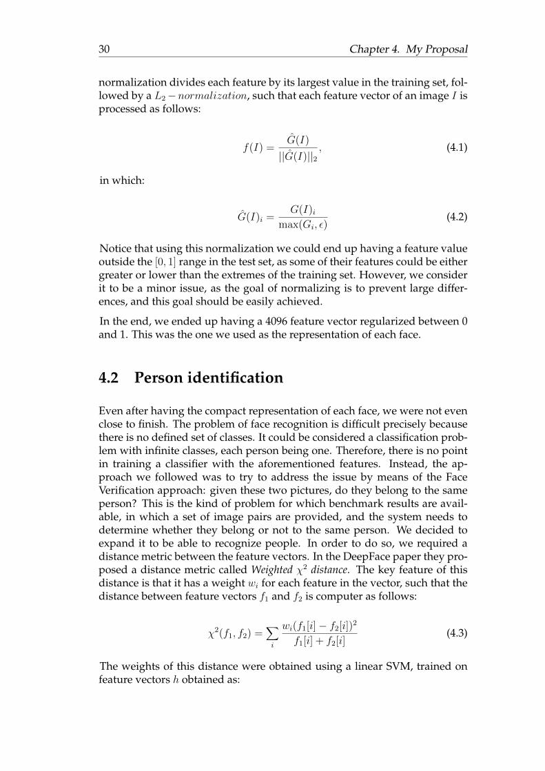
normalization divides each feature by its largest value in the training set, fol-lowed by a L2−normalization, such that each feature vector of an image I isprocessed as follows:
f(I) =G(I)
||G(I)||2, (4.1)
in which:
G(I)i =G(I)i
max(Gi, ε)(4.2)
Notice that using this normalization we could end up having a feature valueoutside the [0, 1] range in the test set, as some of their features could be eithergreater or lower than the extremes of the training set. However, we considerit to be a minor issue, as the goal of normalizing is to prevent large differ-ences, and this goal should be easily achieved.
In the end, we ended up having a 4096 feature vector regularized between 0and 1. This was the one we used as the representation of each face.
4.2 Person identification
Even after having the compact representation of each face, we were not evenclose to finish. The problem of face recognition is difficult precisely becausethere is no defined set of classes. It could be considered a classification prob-lem with infinite classes, each person being one. Therefore, there is no pointin training a classifier with the aforementioned features. Instead, the ap-proach we followed was to try to address the issue by means of the FaceVerification approach: given these two pictures, do they belong to the sameperson? This is the kind of problem for which benchmark results are avail-able, in which a set of image pairs are provided, and the system needs todetermine whether they belong or not to the same person. We decided toexpand it to be able to recognize people. In order to do so, we required adistance metric between the feature vectors. In the DeepFace paper they pro-posed a distance metric called Weighted χ2 distance. The key feature of thisdistance is that it has a weight wi for each feature in the vector, such that thedistance between feature vectors f1 and f2 is computer as follows:
χ2(f1, f2) =∑i
wi(f1[i]− f2[i])2
f1[i] + f2[i](4.3)
The weights of this distance were obtained using a linear SVM, trained onfeature vectors h obtained as:
4.2. Person identification 31
hi =(f1[i] + f2[i])
2
f1[i] + f2[i](4.4)
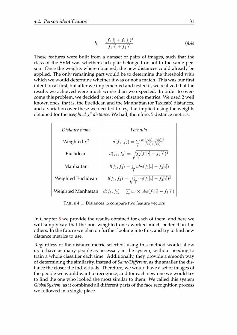
These features were built from a dataset of pairs of images, such that theclass of the SVM was whether each pair belonged or not to the same per-son. Once the weights where obtained, the new distances could already beapplied. The only remaining part would be to determine the threshold withwhich we would determine whether it was or not a match. This was our firstintention at first, but after we implemented and tested it, we realized that theresults we achieved were much worse than we expected. In order to over-come this problem, we decided to test other distance metrics. We used 2 wellknown ones, that is, the Euclidean and the Manhattan (or Taxicab) distances,and a variation over these we decided to try, that implied using the weightsobtained for the weighted χ2 distance. We had, therefore, 5 distance metrics:
Distance name Formula
Weighted χ2 d(f1, f2) =∑i
wi(f1[i]−f2[i])2
f1[i]+f2[i]
Euclidean d(f1, f2) =√∑
i(f1[i]− f2[i])2
Manhattan d(f1, f2) =∑iabs(f1[i]− f2[i])
Weighted Euclidean d(f1, f2) =√∑
iwi(f1[i]− f2[i])2
Weighted Manhattan d(f1, f2) =∑iwi × abs(f1[i]− f2[i])
TABLE 4.1: Distances to compare two feature vectors
In Chapter 5 we provide the results obtained for each of them, and here wewill simply say that the non weighted ones worked much better than theothers. In the future we plan on further looking into this, and try to find newdistance metrics to use.
Regardless of the distance metric selected, using this method would allowus to have as many people as necessary in the system, without needing totrain a whole classifier each time. Additionally, they provide a smooth wayof determining the similarity, instead of Same/Different, as the smaller the dis-tance the closer the individuals. Therefore, we would have a set of images ofthe people we would want to recognize, and for each new one we would tryto find the one who looked the most similar to them. We called this systemGlobalSystem, as it combined all different parts of the face recognition processwe followed in a single place.

32 Chapter 4. My Proposal
4.2.1 GlobalSystem
The GlobalSystem (GS) is composed of two main parts: feature extractionand person identification. The first part has already been explained in Sec-tion 4.1.1, so in this section we will focus in the second part, that is, howexactly do we use these features in order to identify a person, and also howwe trained and tested the whole GS. We have addressed the building of thesystem as an online learner, so that even during the test phase the system canstill learn.
In order to train the GS, a set of labeled people is needed, so that each per-son has its name available. For each of these images, the system processesthem using one of the CNN explained in a previous section − including thefrontalization step − giving 4096 features. Then, it tries to decide whether tokeep it as a representative feature vector or to discard it. In order to do so, wehave a pair of parametres: the minimum number of feature vectors required(Min) and the maximum number allowed (Max). The first one determineshow many images at least we would like to have from each person. There-fore, each time a new feature vector f is received − not only during training−, we check how many feature vectors are already stored from that person. Ifthere are less than Min, the feature vector is always kept. This should allowus to have some variability on that person images to cover different situa-tions (such as expression, facial hair, makeup, etc). If we have more than Minimages, we have to decide whether it is relevant enough to justify keepingit. First of all, we extract the mean (Mean) of all of their feature vectors, andcompare the distance between f and Mean. If it is lower than a previouslyset threshold it means that it resembles some of the images we already have,and so we discard it. Otherwise, we try to determine if it may be an extremeoutlier in which we are not interested, by checking whether the distance isgreater than another threshold. If so, it means that it is an extreme case suchas the ones in Figure 4.5:
FIGURE 4.5: Extreme outliers:Even though all these three pictures belong to the same person,they are hardly recognizable as such. Even more importantly, asthey represent extreme situations that will not likely occur morethan once, they can lead the face recognition system to confusion.They should, therefore, not be kept.

4.2. Person identification 33
As this kind of images can lead the system to confusion, they are discarded.On the contrary, if it falls in between, it means that, even though it may benot be similar to most of the images of that person, it is not so rare as tobe discarded. On the contrary, it can provide interesting information if itcovers a situation that is not covered by other images of the system. Forexample, a smiling face would be necessary if all the stored ones are seriousones. In order to check whether they are indeed interesting, we perform alast comparison. All the images that are close to the mean are considered asthe “average” for that face, and the remaining ones are the valuable outliers.Then, we compare the new image one by one with every outliers to see if theyare considered to belong to the same person (same) or not (different). If therelation |same|/|same + different| is lower than an established proportion,we consider it rare enough so that it is worth keeping. If it is higher, eventhough it may be far from the average image, we already have some similarimages, so we discard it.
Finally, we do not want the system to store an unlimited number of imagesfor every person. Therefore, if the number of stored images is greater than themaximum allowed Max, we have to discard one of them. The one discardedis the closest to the mean of images, as its absence can be easily compensatedby the remaining ones.
By using this mechanism, the GS can determine whether to keep or not thenew image, and this process is followed for every image in the training set.In the future we plan on developing a more complex mechanism, and toperform exhaustive tests on them. In Chapter 5 we provide the results weobtained with this method, as well as the differences when using differentvalues for Min and Max. It is important to notice that this learning processcan also be undertaken during the testing phase.
Then, there is the test phase, that could also be understood as the face recog-nition itself. When given a new picture N , with the person A pictured init, we try to find the closest person to A. In order to do so we have devel-oped different strategies. For each person in the system we will have variousfeature vectors with which to compare the new one.
The first strategy we considered is to choose the person with the closest fea-ture vector. This would assume a “perfect” feature extraction that is capableof taking into account any kind of variations. Even though it worked reason-ably well, it also pose some risks. Let’s assume that A is an average chineseman in sunglasses. On the other hand, we have a similarly aged man (B)who is also chinese, who wears sunglasses in a couple of the stored pictures.If A does no wear sunglasses in any of its stored pictures, it would not beweird for the system to choose B, as the sunglasses could confuse it. Thatbeing said, if each person stored pictures covered a large amount variety ofposes/circumstances, we found out that it provided extremely good results.
The second strategy we considered was to use the one with the smallestmean distance to the stored feature vectors. This tried to address the previ-ous “sunglasses” situation. Unless B wears sunglasses in all stored pictures,

34 Chapter 4. My Proposal
the difference between B without sunglasses and N would likely be largerthan the difference between A without glasses and N . Accordingly, empiri-cal evidences showed that it performed better than simply using the closestone. We also realized that this method delivered good results only whenall faces where in the same conditions − of expression, accessories, etc. Onthe contrary, if person A had a large face variability, new pictures could bemistaken with other people who had a more stable face.
This lead us to the idea of combining both approaches and create a singlemetric that combined them. This metric obtained both the distance to theclosest feature and the mean of all distances, and linearly combined them −with the same weight for each of them. Doing so would, theoretically, solvethe problems of both methods. After testing it, we found out that, in fact,there was no significant improvement over using simply the mean distance.
Finally, we decided to test one last option, which expanded the previous oneby also taking into account the furthest feature. The intuition behind is that,even though you have a large variability between faces, other people couldhave it too, and you will still look more similar to yourself than to others. Inthe end, this approach proved to be the best one, although by a small margin.We plan on developing more complex metrics in the future, possibly givingdifferent weights to each factor.
We must make a clarification, as the performances presented in previousparagraphs correspond to the second set of tests we did. As it will be morethoroughly explained in Chapter 5, we did two kind of tests for these strate-gies. The first one involved less people, and, at first, the dataset had not beenyet cleaned, and it had some incorrectly labeled faces. This made some of thefaces in the dataset either very difficult to process, or simply impossible, asthey did not belong to the person it said they did.Even though we later fixedthese errors, and we obtained more reliable results, it was late in the project.Therefore, the results we first obtained were not nearly as accurate as theones obtained in the second test. In this one we took our time to both auto-matically filter the dataset, and also manually, in order to remove wronglylabeled pictures − the reason for these errors is explained in the followingchapter. Even more, the expanded one has almost 3 times as many people,and almost 5 times more pictures. The behavior of the 4 matching strategiesin both datasets was different similar, but not exactly equal. Taking into ac-count that the second one involves more people, resulting in a more realistictest, we decided to use only the results from the second one.
Summary of GS process We have developed a system capable of perform-ing face recognition, and to continuously learn. It can be trained beforehand,providing a set of labeled images from the people we want it to know. Foreach of these images, it tries to frontalize them and, if it succeeds, it sendsthem through a CNN that extracts a set of 4096 features. These features ana-lyzed to determine whether they could be relevant to keep and, if so, they arepermanently stored in a DB. After the training stage, we have a set of feature
4.2. Person identification 35
vectors for each person in the dataset. These people will be the ones that thesystem will be able to recognize from the first moment.
After that, there is the face recognition phase itself. For each new image,we process them in the same way as the previous ones − including discard-ing them if they have not been properly frontalized. Then, we try to matchit with each of the people stored in the DB, by comparing its feature vectorwith the ones from each of these people. We have different strategies in orderto perform this comparison, and we have yet to reach a conclusion regard-ing which is the most suitable. If no match is found, this new person can bestored into the system, if we want so, so that in the future it will be able torecognize them too. In case a match is found, we can also know the confi-dence of the system. In this case, the feature vector can also be stored if theGS deems it necessary.
It is important to notice that each of these two phases can be performed asmany times as we want to. After having trained the system with a set ofpeople, we can easily repeat the process to add a second batch of people.
In the end, the system is capable of self-adjusting to incorporate new people.The recognition of each person becomes more robust as more time passes, asmore images are available for the system to use.
4.2.2 Technical specifications
In order to implement the system we used Python as programming language.The reasons were that it is really easy to prototype with it, that it has plentyof libraries for mathematical use, and that most of the computational requir-ing ones are implemented in faster languages, so at the end of the day thedifference in performance with respect to languages such as C++ is not thatlarge.
In order to implement the CNN we had many options. The first option weconsidered was to use Google’s Tensorflow [Abadi et al., 2016]. The moti-vation for using it was that, being supported by the, arguably, worldwideleading company in the AI field, it is likely to become a common tool amongAI practitioners. Because of this, we would have liked the opportunity ofgetting familiar with it. Unfortunately, we realized that it did not offer thepossibility of using Locally Connected Layers. As already explained previ-ously in this chapter, these layers are a key feature for our feature extractionmethod, allowing us to obtain different kinds of features at each part of theimage. Therefore, we had to discard it.
The following option we considered was to use the Keras [Chollet, 2015]framework. It easy to use, it has a very active community, and it is con-stantly expanding, so we considered it a good substitute for Tensorflow. Ontop of that, it had the possibility of implementing Locally Connected Layers− which we realized was a rarity among CNN libraries. Interestingly, thispossibility had only been introduced a couple of months before the start of
36 Chapter 4. My Proposal
the project. However, after a pilot test we did on it, we realized that the waythey had implemented these layers was different from the one we required.More concretely, they allowed its use as long as the stride was equal to thefilter size. Therefore, they did not allowed an sliding window which over-laps with each previous position. This made our network, with 3 successiveLocally Connected Layers, impossible to implement with this limitation, asthe image would get reduced to less than a pixel wide.
Finally, we resorted to the pylearn [Goodfellow et al., 2013] library. This onewas developed for academic purposes, and it did not have neither muchsupport nor documentation. However, once we managed to discover howit worked, we were able to use the kind of Locally Connected Layers wewanted. Another important issue was that it allowed the use of GPU. Al-though most libraries allow it, it was important nonetheless. In the end, wewere able to implement the exact network DeepFace proposed−with the ex-ception of the modified input shape−, and to train and test it in a reasonableamount of time − the longest training, with over a million images, took 5days of computation, and processing a single image took slightly more thana second. It also had the advantage that it was extremely easy to integrateit with python, contrary to other libraries, such as convnet, in which it wasmore difficult.
Regarding the frontalization part, we have already explained that we used aface frontalization library, available in Python, that proved to be easy to workand delivered good results in an acceptable amount of time: processing animage and performing the frontalization took less than 2 seconds.
Finally, in order to implement the GS, we needed to be able to permanentlystore the feature vectors, as well as the network’s weights and additionalinformation required by the system. We decided to use MongoDB for this, asit allowed an easy an flexible access to this information that other types ofdatabase would not have. In the end, each GS instance we implemented hadall of its information securely stored in this database, which allowed us toeasily come back to previous experiments and switch between them. Equallyimportant was the speed, as we had to compare each new image with allfeature vectors of that each person in the database. After some testing, wedecided that it did not introduce a significant overhead, even less comparingwith the time it took the CNN and the face frontalization algorithm to processeach image. All in all, for each new image, it takes the GS less than 4 secondsto find a match.
4.3 Real-life examples
In order to test the system with real cases, we developed two applications.The first one was a Web tool to easily train and test a GS. On the other hand,we also incorporated face recognition into a video sequence, which allowedus to process a video and identify who was there, and where. In this section

4.3. Real-life examples 37
we provide a brief explanation of how we have developed each of them, andhow they work.
4.3.1 Web tool
The first practical application in which we used our face recognition systemwas thought as a way of demonstrating its capabilities. In order to do so, wedeveloped a web tool, available from any web browser, that allowed to trainand test a GS of your choice. It relied on a constantly running daemon, in aserver equipped with GPU, so that new images could be processed as fast aspossible. It allowed 3 basic operations:
• Create a GS: The current version of the web tool keeps in memory thelast GS that has been used, and it will be automatically loaded when-ever you access the website. You will be able to recognize people al-ready introduced, or add new ones. Alternatively, you can create a newGS, which you can train with your images. When this option is chosen,the new GS is filled with a default list of 20 celebrities − the completelist can be found in Appendix A−, in order to provide more options totest.
• Train the GS: Regardless of the option chosen, you can add new imagesinto the system. They can belong to people already stored there, inwhich case the system will determine whether they are worthy to bestored. If they belong to people who is not into the system, this will beable to recognize them from now on.
• Test the Gs: The most important feature of the system will be able totest it. For now we have implemented the option of testing a singleimage at a time. After uploading the image, it will look for the bestmatch, and it will return both the name and pictures of that person thatit uses as training. In the future we plan on adding the option of testingmore than one image at once.
A screenshot of the web tool is shown in Figure 4.6:

38 Chapter 4. My Proposal
FIGURE 4.6: The view of the web tool:In this picture there are the 3 available options described above.The screenshot was taken after providing a picture of Obama totest (button “Upload an image”). In the future we plan onallowing testing with multiple images at once. [Serra, 2016]
4.3.2 Video recognition
The second application was more practical. Given a video with a personin it, it was capable of following and recognizing them. After each video isprocessed, the bounding box of the face is drawn, and the name of the personin it is written at its top left corner. In order to do so, we locate the mostpromising bounding box at each frame, by using a Faster R-CNN, and eachsecond we use a GS to detect the person in it. The low frequency of detectionaims to reduce the processing time. After the whole video is processed, weselect the most probable match from all the predicted ones. By doing so,predictions become very robust, as we minimize the probability of a miss-classification. We are currently improving it in order to allow detection ofmultiple people. In order to do so, we use flow motion to “follow” the facesduring the video, but it is still not properly working. An example of someframes of a processed video can be seen in Figure 4.7

4.3. Real-life examples 39
FIGURE 4.7: Face Recognition applied to video

41
Chapter 5
Experiments and Results
In order to train and test our system, we required a large amount of labeledfaces. In the test phase, we evaluated it in two different problems, face ver-ification and face recognition. In this section we provide a description of thedataset we used, the settings of the experiments we performed, and the re-sults obtained.
5.1 Datasets
CNNs require a lot of data to be trained. As an example, DeepFace wastrained using a dataset containing over 4.4 million images. As it was a privateone, we did not have access to it, nor we could gather that many fast enough,so we decided to look for public datasets that could help us. Unfortunately,we realized that none of the publicly available ones are large enough, beingthe largest one around a couple hundreds of thousands. In order to addressthis issue, we resolved to combine different public datasets into a single oneto maximize the number of available images. Concretely, the used ones wereCasia [Yi et al., 2014], CACD [Chen, Chen, and Hsu, 2014] and FaceScrub [Ngand Winkler, 2014]. We also used images that we the company had gatheredvia web scrapping. The three datasets used were the largest public ones,and together with the gathered ones, they provided around 700,000 RGB im-ages, labeled with the name of the depicted person. This number was stillfar away from the ones from DeepFace, but we considered that they wouldbe enough for, at least, test the system. Once the system is working, we willfocus on gathering images of our own, so that we get closer to the millionsfrom DeepFace, by using a semi-supervised method [Parkhi, Vedaldi, andZisserman, 2015].
From the initial 700,000 images we had, we ended up having slightly lessthan 600,000 when we discarded the unusable ones, as explained in previouschapter. From those, there may be some repeated ones, as they came fromdifferent datasets, but we did not have the means for checking them individ-ually. We decided to accept it, as they were likely to be few, in comparisonwith the correct ones. We decided to use 500,000 as the training set for boththe CNN and the GS, and the remaining 100,000 for testing. In order to test
42 Chapter 5. Experiments and Results
the system as thoroughly as possible, and to prevent overfitting the train-ing set, none of the people in the test set were also in the training one. The500,000 training images belong to 9351 different people, and the ones in thetest set account for 1671 additional ones.
One additional problem was that these datasets are generated in a semi-automatic way. This lead to some of the faces being improperly labeled, ornot being usable. These cases included faces from people who resembledthem, but also drawings, or people related with them. For example, someactors had fellow actors from films in which they worked together. In one ofthe most outstanding case, the actress Amy Sedaris, who had voiced a char-acter in the Shrek film, had a picture of Shrek as one of her pictures. Thisproblem was partly solved in the filtering process, which discarded draw-ings and similar cases. However, there was still some cases we could notaddress unless we manually checked each of them. As this was not feasible,we decided to also accept it. These problems remained to be solved in thefuture by having better treated datasets.
Apart from that, we decided the use the Labeled Faces in the Wild (LFW) [Huanget al., 2007] dataset as a benchmark to check the performance of our CNN.Precisely, DeepFace is one of the systems that uses this dataset as a bench-mark, so it was logical for use to use. This dataset contains 13,000 imagesof labeled celebrities, and it is commonly used to assess the performance offace recognition systems. This assessment does not, strictly speaking, cor-respond to face recognition performance, but rather to face verification, asexplained in following Section 5.1.1. There is, however, a remark regardingthis dataset. As it is a relatively small one, having only 1000 test samples,current state-of-art methods are already close to 100% of accuracy. On top ofit, human performance is set around 97.53%, threshold that has already beensurpassed by some methods. Therefore, any improvement over current stateof art corresponds to very controversial cases, and so is difficult to properlyasses the performance of new methods. In order to address this issue, thereis a general belief that larger benchmark datasets should be generated. How-ever, for the time being LFW is the most used by far, even by DeepFace, sowe have decided to use it nevertheless.
Additionally, we decided to generate two new image datasets from the oneswe had by applying transformations on the images. The process we followedis presented in Section 5.1.2.
5.1.1 Face Verification
Face verification differs from the face recognition in that, in the latter, theproblem consists in knowing who is there in the picture, whereas in the for-mer, given two pictures, the goal is to determine whether they belong or notto the same person. Therefore, in the LFW dataset, they provide two lists ofpairs of images. Each pair of images can belong to the same person or not,and there is the same number of each of them. One list is used for training,
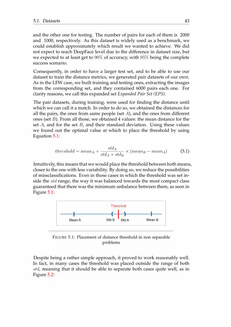
5.1. Datasets 43
and the other one for testing. The number of pairs for each of them is 2000and 1000, respectively. As this dataset is widely used as a benchmark, wecould establish approximately which result we wanted to achieve. We didnot expect to reach DeepFace level due to the difference in dataset size, butwe expected to at least get to 90% of accuracy, with 95% being the completesuccess scenario.
Consequently, in order to have a larger test set, and to be able to use ourdataset to train the distance metrics, we generated pair datasets of our own.As in the LFW case, we built training and testing ones, extracting the imagesfrom the corresponding set, and they contained 6000 pairs each one. Forclarity reasons, we call this expanded set Expanded Pair Set (EPS).
The pair datasets, during training, were used for finding the distance untilwhich we can call it a match. In order to do so, we obtained the distances forall the pairs, the ones from same people (set A), and the ones from differentones (set B). From all those, we obtained 4 values: the mean distance for theset A, and for the set B, and their standard deviation. Using these valueswe found out the optimal value at which to place the threshold by usingEquation 5.1:
threshold = meanA +stdA
stdA + stdB× (meanB −meanA) (5.1)
Intuitively, this means that we would place the threshold between both means,closer to the one with less variability. By doing so, we reduce the possibilitiesof missclassifications. Even in those cases in which the threshold was set in-side the std range, the way it was balanced towards the most compact classguaranteed that there was the minimum unbalance between them, as seen inFigure 5.1:
FIGURE 5.1: Placement of distance threshold in non separableproblems
Despite being a rather simple approach, it proved to work reasonably well.In fact, in many cases the threshold was placed outside the range of bothstd, meaning that it should be able to separate both cases quite well, as inFigure 5.2:
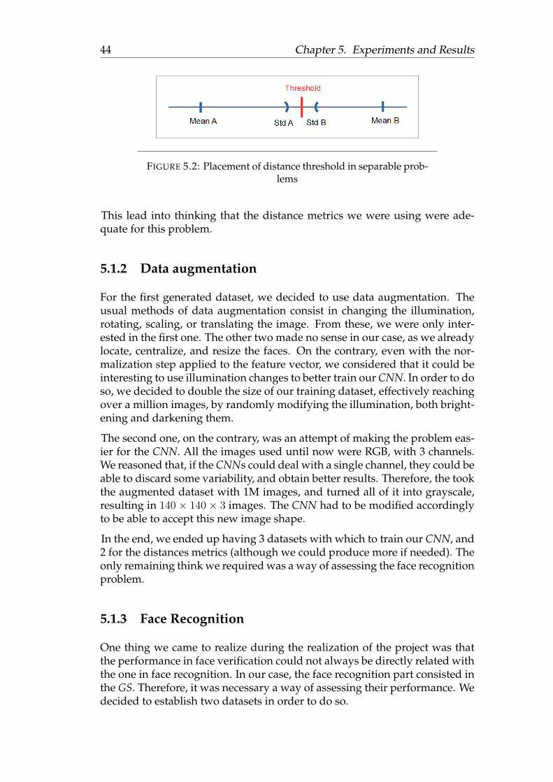
44 Chapter 5. Experiments and Results
FIGURE 5.2: Placement of distance threshold in separable prob-lems
This lead into thinking that the distance metrics we were using were ade-quate for this problem.
5.1.2 Data augmentation
For the first generated dataset, we decided to use data augmentation. Theusual methods of data augmentation consist in changing the illumination,rotating, scaling, or translating the image. From these, we were only inter-ested in the first one. The other two made no sense in our case, as we alreadylocate, centralize, and resize the faces. On the contrary, even with the nor-malization step applied to the feature vector, we considered that it could beinteresting to use illumination changes to better train our CNN. In order to doso, we decided to double the size of our training dataset, effectively reachingover a million images, by randomly modifying the illumination, both bright-ening and darkening them.
The second one, on the contrary, was an attempt of making the problem eas-ier for the CNN. All the images used until now were RGB, with 3 channels.We reasoned that, if the CNNs could deal with a single channel, they could beable to discard some variability, and obtain better results. Therefore, the tookthe augmented dataset with 1M images, and turned all of it into grayscale,resulting in 140 × 140 × 3 images. The CNN had to be modified accordinglyto be able to accept this new image shape.
In the end, we ended up having 3 datasets with which to train our CNN, and2 for the distances metrics (although we could produce more if needed). Theonly remaining think we required was a way of assessing the face recognitionproblem.
5.1.3 Face Recognition
One thing we came to realize during the realization of the project was thatthe performance in face verification could not always be directly related withthe one in face recognition. In our case, the face recognition part consisted inthe GS. Therefore, it was necessary a way of assessing their performance. Wedecided to establish two datasets in order to do so.
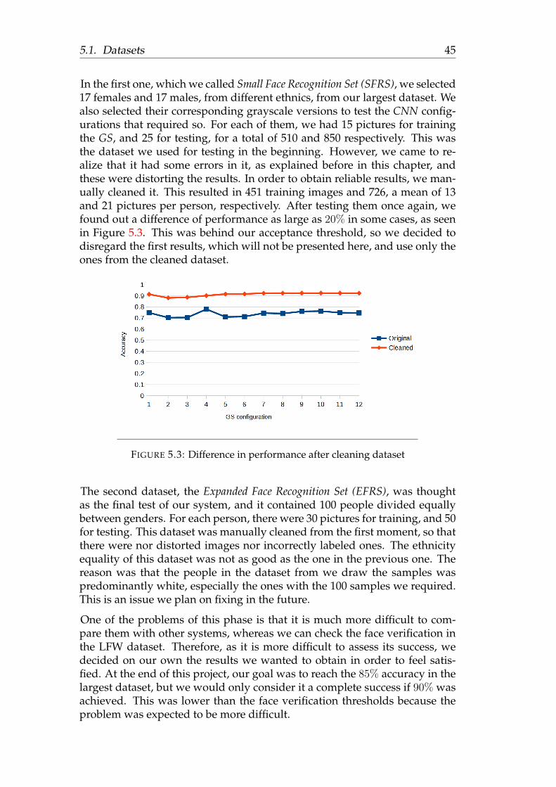
5.1. Datasets 45
In the first one, which we called Small Face Recognition Set (SFRS), we selected17 females and 17 males, from different ethnics, from our largest dataset. Wealso selected their corresponding grayscale versions to test the CNN config-urations that required so. For each of them, we had 15 pictures for trainingthe GS, and 25 for testing, for a total of 510 and 850 respectively. This wasthe dataset we used for testing in the beginning. However, we came to re-alize that it had some errors in it, as explained before in this chapter, andthese were distorting the results. In order to obtain reliable results, we man-ually cleaned it. This resulted in 451 training images and 726, a mean of 13and 21 pictures per person, respectively. After testing them once again, wefound out a difference of performance as large as 20% in some cases, as seenin Figure 5.3. This was behind our acceptance threshold, so we decided todisregard the first results, which will not be presented here, and use only theones from the cleaned dataset.
FIGURE 5.3: Difference in performance after cleaning dataset
The second dataset, the Expanded Face Recognition Set (EFRS), was thoughtas the final test of our system, and it contained 100 people divided equallybetween genders. For each person, there were 30 pictures for training, and 50for testing. This dataset was manually cleaned from the first moment, so thatthere were nor distorted images nor incorrectly labeled ones. The ethnicityequality of this dataset was not as good as the one in the previous one. Thereason was that the people in the dataset from we draw the samples waspredominantly white, especially the ones with the 100 samples we required.This is an issue we plan on fixing in the future.
One of the problems of this phase is that it is much more difficult to com-pare them with other systems, whereas we can check the face verification inthe LFW dataset. Therefore, as it is more difficult to assess its success, wedecided on our own the results we wanted to obtain in order to feel satis-fied. At the end of this project, our goal was to reach the 85% accuracy in thelargest dataset, but we would only consider it a complete success if 90% wasachieved. This was lower than the face verification thresholds because theproblem was expected to be more difficult.
46 Chapter 5. Experiments and Results
5.2 Experiments Description
The experiments we performed had many goals. We had multiple separateelements to test, which were:
• CNN configurations: The CNN we used was the one they provided inthe DeepFace paper. Therefore, we did not have to look for the bestconfiguration. However, as explained in previous chapter, we decidedto implement a reduced version of the network, in an attempt to re-duce the possible overfitting. This reduced dataset had one less LocallyConnected Layer than the original, as these layers imply a large num-ber of additional parameters to learn. We also decided tested differentdropout rates, as these can also help in reducing the overfitting
• Similarity measures: Given two feature vectors, we had to comparethem in order to determine whether they belong or not to the sameperson. This was achieved by means of a distance measure. Given the5 possibilities we considered, we had to train and test each of them. Wedecided to perform these in two datasets: the LFW and the EPS. Foreach of them, we performed training to determine the exact thresholddistance from which to accept a match, and then we would use theresulting threshold to test it.
• GS strategies: Given the CNN and the similarity measure, we are ableto determine whether two pictures belong to the same person. As al-ready explained in previous chapter, each person would have morethan one feature vector stored in the GS. In order to determine whothe new picture belongs to, we have different strategies to do so. Theyhave already been explained, so as a summary we have: using the clos-est feature vector, the mean of the distances, combining both of thesevalues, and considering also the furthest feature vector. On top of that,we also wanted to test different values for the maximum and minimumnumber of stored images per per person.
Experiment pyramid In the end we ended having a large number of pos-sible combinations. Testing each of them was not feasible due to time con-straints, so we decided to perform a pyramid-like chain of experiments. Wewould have a set of successive experiments, instead of a single one. At eachstage, we would drop some possibilities, until we only had a small numberof possibilities to test. The goal would be to test 4 CNN configurations in 3datasets, resulting in 12 CNNs. The datasets would be the 500,000 imagesretrieved, the augmented 1M, and the grayscale ones. For each of them, wewould test the CNN configuration proposed in the DeepFace paper, and thereduced version. Finally, in these two configurations we would use a dropoutrate of 0.5 and 0.7, and see which worked better. In order to test them, wewould perform the following chain of experiments:
1. In the first step we would train the 12 CNN configurations.
5.3. CNN training 47
2. Then, we would address the face verification problem. The Euclideanand Taxicab distances would be trained in the LFW pair sets, and wewould use the obtained threshold to test them. We did not use theweighted distances at this step because they required to train a SVM,and we considered that the 2000 training pairs might not be enough. Inthe end, this would provide us 24 values.
3. In the second step, and continuing with the face verification problem,we had a double goal. The first one was to test the weighted distancesin all the CNN configurations, resulting in 36 values. On the other hand,we would select the combinations of distances and CNN configurationsthat performed the best in the LFW dataset, and keep only the best halffor each dataset, which accounted for 12 combinations. In the end, 48results.
4. At this step we would switch to the face recognition problem, by testingdifferent GS. From the 48 previous values, we would select only thebest 1/4. For each of these we would test a total of 8 GS configurations,according to the factors previously explained in this chapter. In orderto perform this test, we used the smaller of the two face recognitionsets we had, to speed the process. In the end, 96 results were obtained.Instead on focusing on the GS configurations, we decided to focus onfinding the combinations of CNN and distance metrics that obtainedthe best results in average, and rely in the next step to decide the GSitself.
5. For the final step, we took the best, in average, 6 CNN and distancemetrics from previous step. Each of them was tested in the more com-plete face recognition dataset, and the obtained results were the oneswe selected as definitive.
The experiments were all performed in GPU provided servers, which al-lowed us to finish them in a reasonable amount of time. All in all, we spentapproximately a month and a half testing the system, with multiple tests be-ing run in parallel.
5.3 CNN training
In order to train the CNN, we followed a similar configuration to the oneproposed in the DeepFace paper. We used Stochastic Gradient Descent inorder to train the CNN, not only because it was used in the paper, but alsobecause it is indicated for this kind of networks. The momentum used was0.9, and the batch size was 128. The starting learning rate was set to 0.001,and we made it gradually decrease until reaching 0.0001. Each network wastrained for 15 epochs. All weights were drawn from a Gaussian distributionwith µ = 0 and σ = 0.01. The longest training took 5 days, and it was the oneinvolving 1M RGB images. The one with 500,000 RGB images took 2 and ahalf days.

48 Chapter 5. Experiments and Results
One of the pending tasks we had was to use a pre-trained network. Labeledfaces are not easy to find, but it is easier to find labelel images of animalsor objects. We plan on gathering a large amount − larger than our currentdatasets− of this kind of image, and use them to pre-train the network. Afterthat, we will fine-tune the network with our face dataset. This is a commonstrategy for training CNN when little data is available. We did not attemptto do so due to 2 reasons. First, we were not sure that our amount of datawas not enough for, at least, getting acceptable results to test. Second, if wehad done it we may have not been able to get as far as we wanted with thedevelopment of the whole face recognition system. Now that it is up andrunning, any improvement on the CNNs will benefit the GS.
5.4 Results
In this section we provide the results we obtained in the experiments. Someof these results will be presented as graphs, in which to see the relation be-tween performance and some of the parameters previously mentioned.
5.4.1 LFW
First of all, we introduce the results we obtained in the LFW dataset. Thesewere interesting because we could compare them with the ones obtained byDeeFace, which will provide a good comparison of the difference in perfor-mance. The results we present were obtained using the Euclidean and theTaxicab distance to compare the feature vectors produced by the CNN, asalready explained.
We had 12 CNN trained, and we tested all of them in the LFW, using the twodistance metrics, resulting in 24 values. In Table 5.3 we present these results.The green cell corresponds to the best accuracy achieved:
Even though we got results above the 80% in accuracy in all cases, with amaximum of 89.6%, but we did not reach the 90% we wanted. Comparingwith other methods, such as the ones in Table 5.1, we we were quite behind.
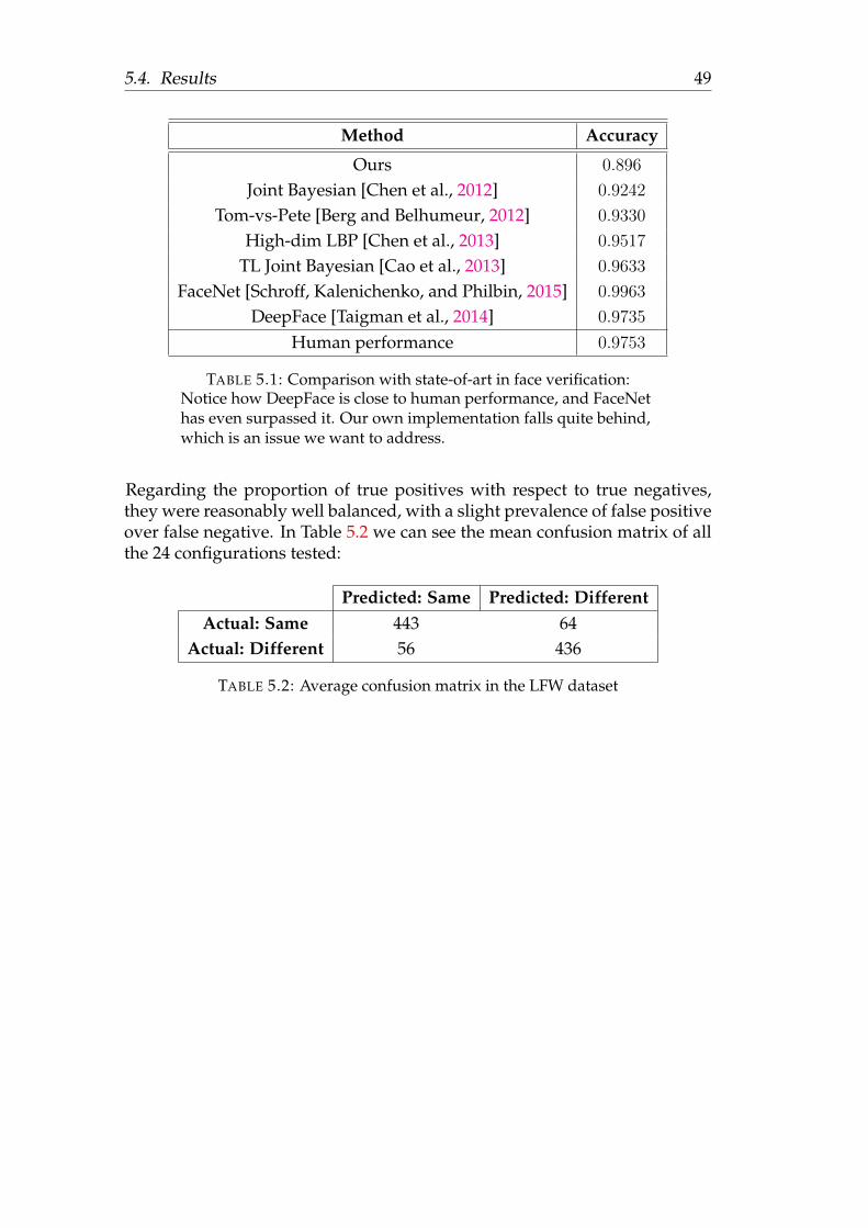
5.4. Results 49
Method Accuracy
Ours 0.896
Joint Bayesian [Chen et al., 2012] 0.9242
Tom-vs-Pete [Berg and Belhumeur, 2012] 0.9330
High-dim LBP [Chen et al., 2013] 0.9517
TL Joint Bayesian [Cao et al., 2013] 0.9633
FaceNet [Schroff, Kalenichenko, and Philbin, 2015] 0.9963
DeepFace [Taigman et al., 2014] 0.9735
Human performance 0.9753
TABLE 5.1: Comparison with state-of-art in face verification:Notice how DeepFace is close to human performance, and FaceNethas even surpassed it. Our own implementation falls quite behind,which is an issue we want to address.
Regarding the proportion of true positives with respect to true negatives,they were reasonably well balanced, with a slight prevalence of false positiveover false negative. In Table 5.2 we can see the mean confusion matrix of allthe 24 configurations tested:
Predicted: Same Predicted: DifferentActual: Same 443 64
Actual: Different 56 436
TABLE 5.2: Average confusion matrix in the LFW dataset
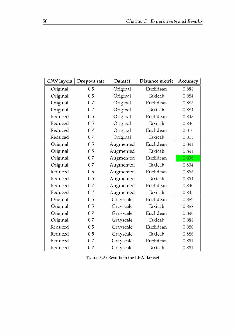
50 Chapter 5. Experiments and Results
CNN layers Dropout rate Dataset Distance metric Accuracy
Original 0.5 Original Euclidean 0.888
Original 0.5 Original Taxicab 0.884
Original 0.7 Original Euclidean 0.885
Original 0.7 Original Taxicab 0.884
Reduced 0.5 Original Euclidean 0.843
Reduced 0.5 Original Taxicab 0.846
Reduced 0.7 Original Euclidean 0.816
Reduced 0.7 Original Taxicab 0.813
Original 0.5 Augmented Euclidean 0.891
Original 0.5 Augmented Taxicab 0.891
Original 0.7 Augmented Euclidean 0.896
Original 0.7 Augmented Taxicab 0.894
Reduced 0.5 Augmented Euclidean 0.855
Reduced 0.5 Augmented Taxicab 0.854
Reduced 0.7 Augmented Euclidean 0.846
Reduced 0.7 Augmented Taxicab 0.845
Original 0.5 Grayscale Euclidean 0.889
Original 0.5 Grayscale Taxicab 0.888
Original 0.7 Grayscale Euclidean 0.890
Original 0.7 Grayscale Taxicab 0.888
Reduced 0.5 Grayscale Euclidean 0.880
Reduced 0.5 Grayscale Taxicab 0.886
Reduced 0.7 Grayscale Euclidean 0.861
Reduced 0.7 Grayscale Taxicab 0.861
TABLE 5.3: Results in the LFW dataset
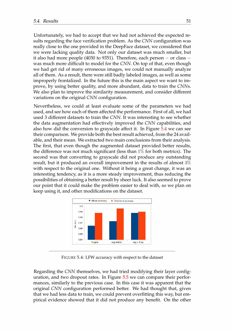
5.4. Results 51
Unfortunately, we had to accept that we had not achieved the expected re-sults regarding the face verification problem. As the CNN configuration wasreally close to the one provided in the DeepFace dataset, we considered thatwe were lacking quality data. Not only our dataset was much smaller, butit also had more people (4030 to 9351). Therefore, each person − or class −was much more difficult to model for the CNN. On top of that, even thoughwe had get rid of many erroneous images, we could not manually analyzeall of them. As a result, there were still badly labeled images, as well as someimproperly frontalized. In the future this is the main aspect we want to im-prove, by using better quality, and more abundant, data to train the CNNs.We also plan to improve the similarity measurement, and consider differentvariations on the original CNN configuration.
Nevertheless, we could at least evaluate some of the parameters we hadused, and see how each of them affected the performance. First of all, we hadused 3 different datasets to train the CNN. It was interesting to see whetherthe data augmentation had effectively improved the CNN capabilities, andalso how did the conversion to grayscale affect it. In Figure 5.4 we can seetheir comparison. We provide both the best result achieved, from the 24 avail-able, and their mean. We extracted two main conclusions from their analysis.The first, that even though the augmented dataset provided better results,the difference was not much significant (less than 1% for both metrics). Thesecond was that converting to grayscale did not produce any outstandingresult, but it produced an overall improvement in the results of almost 3%with respect to the original one. Without it being a great change, it was aninteresting tendency, as it is a more steady improvement, thus reducing thepossibilities of obtaining a better result by sheer luck. It also seemed to proveour point that it could make the problem easier to deal with, so we plan onkeep using it, and other modifications on the dataset.
FIGURE 5.4: LFW accuracy with respect to the dataset
Regarding the CNN themselves, we had tried modifying their layer config-uration, and two dropout rates. In Figure 5.5 we can compare their perfor-mances, similarly to the previous case. In this case it was apparent that theoriginal CNN configuration performed better. We had thought that, giventhat we had less data to train, we could prevent overfitting this way, but em-pirical evidence showed that it did not produce any benefit. On the other
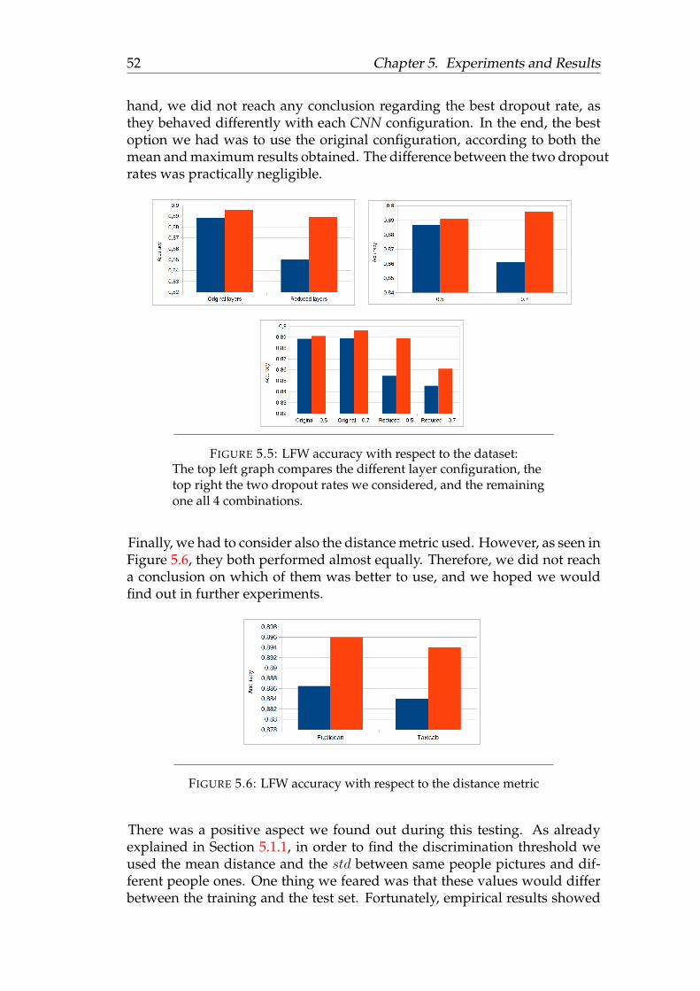
52 Chapter 5. Experiments and Results
hand, we did not reach any conclusion regarding the best dropout rate, asthey behaved differently with each CNN configuration. In the end, the bestoption we had was to use the original configuration, according to both themean and maximum results obtained. The difference between the two dropoutrates was practically negligible.
FIGURE 5.5: LFW accuracy with respect to the dataset:The top left graph compares the different layer configuration, thetop right the two dropout rates we considered, and the remainingone all 4 combinations.
Finally, we had to consider also the distance metric used. However, as seen inFigure 5.6, they both performed almost equally. Therefore, we did not reacha conclusion on which of them was better to use, and we hoped we wouldfind out in further experiments.
FIGURE 5.6: LFW accuracy with respect to the distance metric
There was a positive aspect we found out during this testing. As alreadyexplained in Section 5.1.1, in order to find the discrimination threshold weused the mean distance and the std between same people pictures and dif-ferent people ones. One thing we feared was that these values would differbetween the training and the test set. Fortunately, empirical results showed
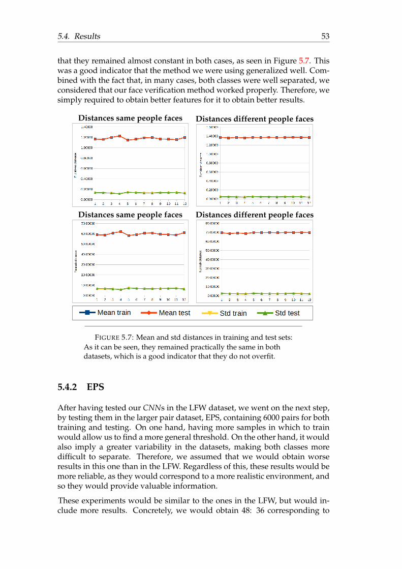
5.4. Results 53
that they remained almost constant in both cases, as seen in Figure 5.7. Thiswas a good indicator that the method we were using generalized well. Com-bined with the fact that, in many cases, both classes were well separated, weconsidered that our face verification method worked properly. Therefore, wesimply required to obtain better features for it to obtain better results.
Distances same people faces Distances different people faces
Distances same people faces Distances different people faces
FIGURE 5.7: Mean and std distances in training and test sets:As it can be seen, they remained practically the same in bothdatasets, which is a good indicator that they do not overfit.
5.4.2 EPS
After having tested our CNNs in the LFW dataset, we went on the next step,by testing them in the larger pair dataset, EPS, containing 6000 pairs for bothtraining and testing. On one hand, having more samples in which to trainwould allow us to find a more general threshold. On the other hand, it wouldalso imply a greater variability in the datasets, making both classes moredifficult to separate. Therefore, we assumed that we would obtain worseresults in this one than in the LFW. Regardless of this, these results would bemore reliable, as they would correspond to a more realistic environment, andso they would provide valuable information.
These experiments would be similar to the ones in the LFW, but would in-clude more results. Concretely, we would obtain 48: 36 corresponding to
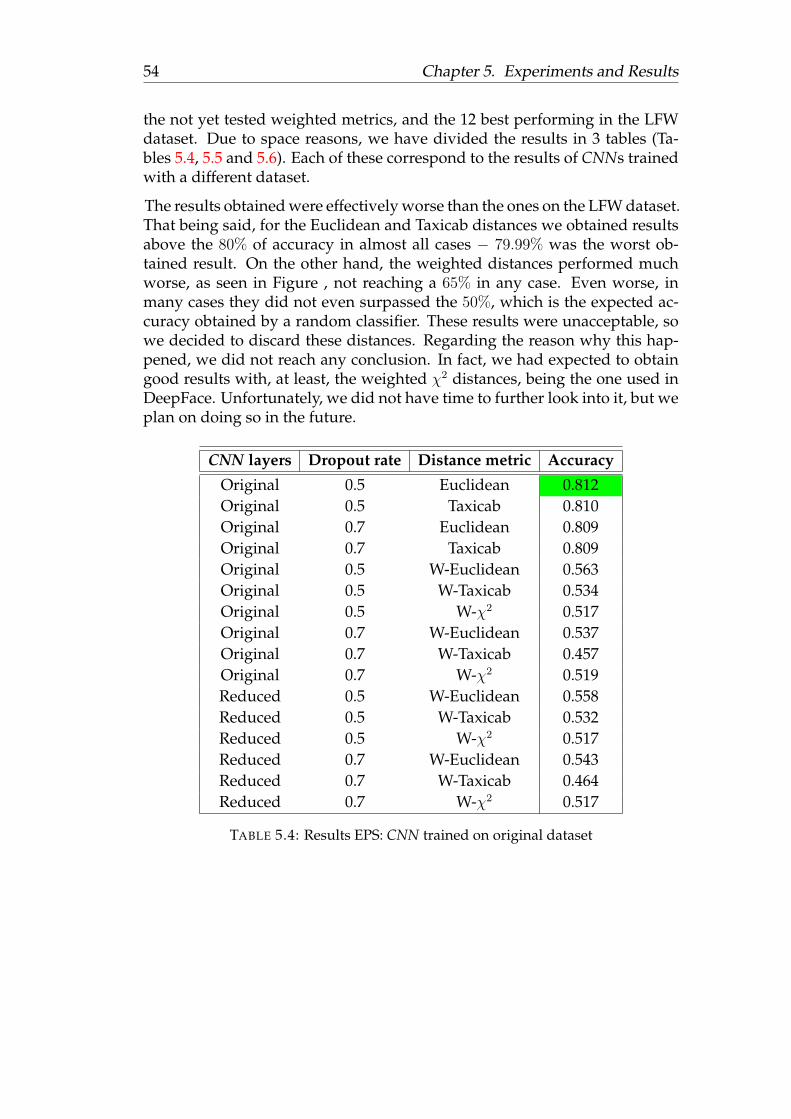
54 Chapter 5. Experiments and Results
the not yet tested weighted metrics, and the 12 best performing in the LFWdataset. Due to space reasons, we have divided the results in 3 tables (Ta-bles 5.4, 5.5 and 5.6). Each of these correspond to the results of CNNs trainedwith a different dataset.
The results obtained were effectively worse than the ones on the LFW dataset.That being said, for the Euclidean and Taxicab distances we obtained resultsabove the 80% of accuracy in almost all cases − 79.99% was the worst ob-tained result. On the other hand, the weighted distances performed muchworse, as seen in Figure , not reaching a 65% in any case. Even worse, inmany cases they did not even surpassed the 50%, which is the expected ac-curacy obtained by a random classifier. These results were unacceptable, sowe decided to discard these distances. Regarding the reason why this hap-pened, we did not reach any conclusion. In fact, we had expected to obtaingood results with, at least, the weighted χ2 distances, being the one used inDeepFace. Unfortunately, we did not have time to further look into it, but weplan on doing so in the future.
CNN layers Dropout rate Distance metric Accuracy
Original 0.5 Euclidean 0.812Original 0.5 Taxicab 0.810Original 0.7 Euclidean 0.809Original 0.7 Taxicab 0.809Original 0.5 W-Euclidean 0.563Original 0.5 W-Taxicab 0.534Original 0.5 W-χ2 0.517Original 0.7 W-Euclidean 0.537Original 0.7 W-Taxicab 0.457Original 0.7 W-χ2 0.519Reduced 0.5 W-Euclidean 0.558Reduced 0.5 W-Taxicab 0.532Reduced 0.5 W-χ2 0.517Reduced 0.7 W-Euclidean 0.543Reduced 0.7 W-Taxicab 0.464Reduced 0.7 W-χ2 0.517
TABLE 5.4: Results EPS: CNN trained on original dataset
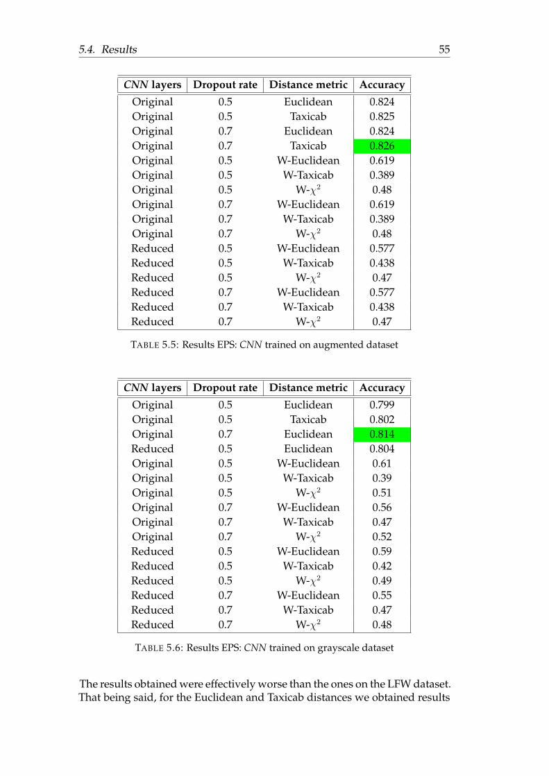
5.4. Results 55
CNN layers Dropout rate Distance metric Accuracy
Original 0.5 Euclidean 0.824Original 0.5 Taxicab 0.825Original 0.7 Euclidean 0.824Original 0.7 Taxicab 0.826Original 0.5 W-Euclidean 0.619Original 0.5 W-Taxicab 0.389Original 0.5 W-χ2 0.48Original 0.7 W-Euclidean 0.619Original 0.7 W-Taxicab 0.389Original 0.7 W-χ2 0.48Reduced 0.5 W-Euclidean 0.577Reduced 0.5 W-Taxicab 0.438Reduced 0.5 W-χ2 0.47Reduced 0.7 W-Euclidean 0.577Reduced 0.7 W-Taxicab 0.438Reduced 0.7 W-χ2 0.47
TABLE 5.5: Results EPS: CNN trained on augmented dataset
CNN layers Dropout rate Distance metric Accuracy
Original 0.5 Euclidean 0.799Original 0.5 Taxicab 0.802Original 0.7 Euclidean 0.814Reduced 0.5 Euclidean 0.804Original 0.5 W-Euclidean 0.61Original 0.5 W-Taxicab 0.39Original 0.5 W-χ2 0.51Original 0.7 W-Euclidean 0.56Original 0.7 W-Taxicab 0.47Original 0.7 W-χ2 0.52Reduced 0.5 W-Euclidean 0.59Reduced 0.5 W-Taxicab 0.42Reduced 0.5 W-χ2 0.49Reduced 0.7 W-Euclidean 0.55Reduced 0.7 W-Taxicab 0.47Reduced 0.7 W-χ2 0.48
TABLE 5.6: Results EPS: CNN trained on grayscale dataset
The results obtained were effectively worse than the ones on the LFW dataset.That being said, for the Euclidean and Taxicab distances we obtained results
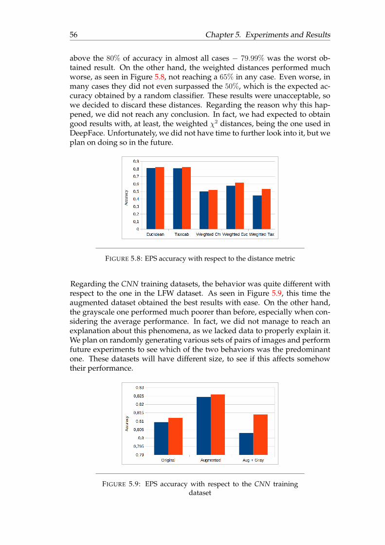
56 Chapter 5. Experiments and Results
above the 80% of accuracy in almost all cases − 79.99% was the worst ob-tained result. On the other hand, the weighted distances performed muchworse, as seen in Figure 5.8, not reaching a 65% in any case. Even worse, inmany cases they did not even surpassed the 50%, which is the expected ac-curacy obtained by a random classifier. These results were unacceptable, sowe decided to discard these distances. Regarding the reason why this hap-pened, we did not reach any conclusion. In fact, we had expected to obtaingood results with, at least, the weighted χ2 distances, being the one used inDeepFace. Unfortunately, we did not have time to further look into it, but weplan on doing so in the future.
FIGURE 5.8: EPS accuracy with respect to the distance metric
Regarding the CNN training datasets, the behavior was quite different withrespect to the one in the LFW dataset. As seen in Figure 5.9, this time theaugmented dataset obtained the best results with ease. On the other hand,the grayscale one performed much poorer than before, especially when con-sidering the average performance. In fact, we did not manage to reach anexplanation about this phenomena, as we lacked data to properly explain it.We plan on randomly generating various sets of pairs of images and performfuture experiments to see which of the two behaviors was the predominantone. These datasets will have different size, to see if this affects somehowtheir performance.
FIGURE 5.9: EPS accuracy with respect to the CNN trainingdataset
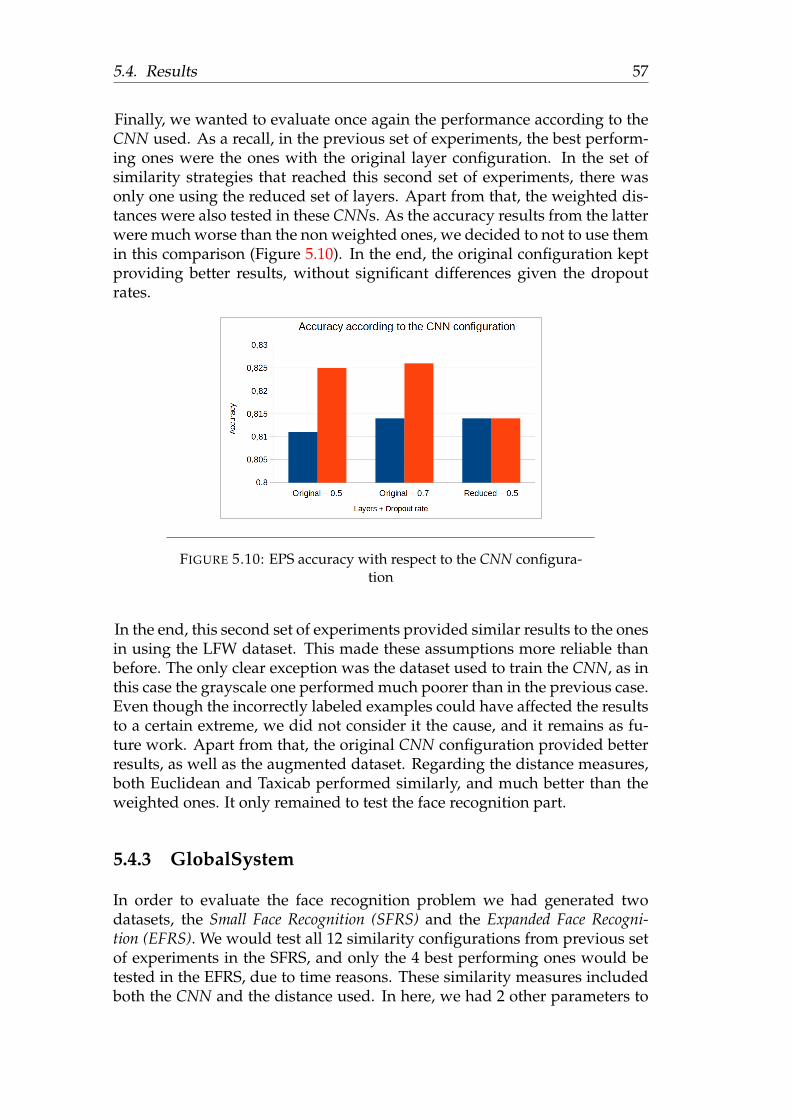
5.4. Results 57
Finally, we wanted to evaluate once again the performance according to theCNN used. As a recall, in the previous set of experiments, the best perform-ing ones were the ones with the original layer configuration. In the set ofsimilarity strategies that reached this second set of experiments, there wasonly one using the reduced set of layers. Apart from that, the weighted dis-tances were also tested in these CNNs. As the accuracy results from the latterwere much worse than the non weighted ones, we decided to not to use themin this comparison (Figure 5.10). In the end, the original configuration keptproviding better results, without significant differences given the dropoutrates.
FIGURE 5.10: EPS accuracy with respect to the CNN configura-tion
In the end, this second set of experiments provided similar results to the onesin using the LFW dataset. This made these assumptions more reliable thanbefore. The only clear exception was the dataset used to train the CNN, as inthis case the grayscale one performed much poorer than in the previous case.Even though the incorrectly labeled examples could have affected the resultsto a certain extreme, we did not consider it the cause, and it remains as fu-ture work. Apart from that, the original CNN configuration provided betterresults, as well as the augmented dataset. Regarding the distance measures,both Euclidean and Taxicab performed similarly, and much better than theweighted ones. It only remained to test the face recognition part.
5.4.3 GlobalSystem
In order to evaluate the face recognition problem we had generated twodatasets, the Small Face Recognition (SFRS) and the Expanded Face Recogni-tion (EFRS). We would test all 12 similarity configurations from previous setof experiments in the SFRS, and only the 4 best performing ones would betested in the EFRS, due to time reasons. These similarity measures includedboth the CNN and the distance used. In here, we had 2 other parameters to
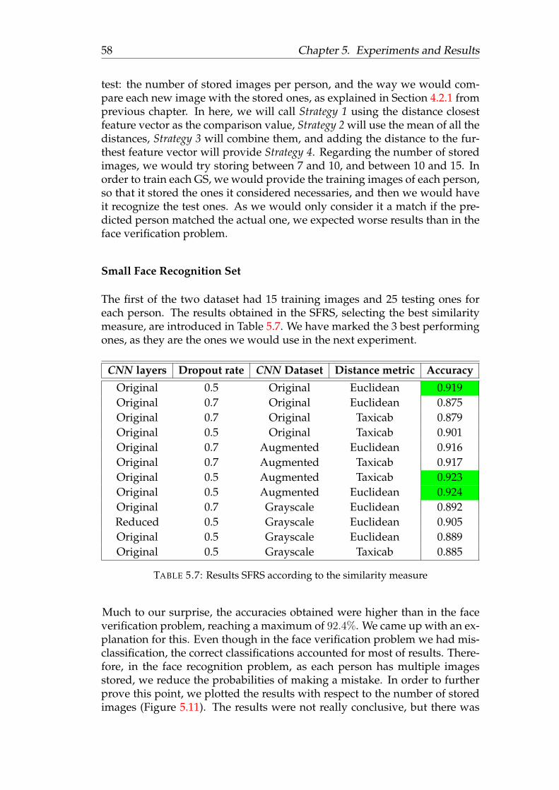
58 Chapter 5. Experiments and Results
test: the number of stored images per person, and the way we would com-pare each new image with the stored ones, as explained in Section 4.2.1 fromprevious chapter. In here, we will call Strategy 1 using the distance closestfeature vector as the comparison value, Strategy 2 will use the mean of all thedistances, Strategy 3 will combine them, and adding the distance to the fur-thest feature vector will provide Strategy 4. Regarding the number of storedimages, we would try storing between 7 and 10, and between 10 and 15. Inorder to train each GS, we would provide the training images of each person,so that it stored the ones it considered necessaries, and then we would haveit recognize the test ones. As we would only consider it a match if the pre-dicted person matched the actual one, we expected worse results than in theface verification problem.
Small Face Recognition Set
The first of the two dataset had 15 training images and 25 testing ones foreach person. The results obtained in the SFRS, selecting the best similaritymeasure, are introduced in Table 5.7. We have marked the 3 best performingones, as they are the ones we would use in the next experiment.
CNN layers Dropout rate CNN Dataset Distance metric Accuracy
Original 0.5 Original Euclidean 0.919Original 0.7 Original Euclidean 0.875Original 0.7 Original Taxicab 0.879Original 0.5 Original Taxicab 0.901Original 0.7 Augmented Euclidean 0.916Original 0.7 Augmented Taxicab 0.917Original 0.5 Augmented Taxicab 0.923Original 0.5 Augmented Euclidean 0.924Original 0.7 Grayscale Euclidean 0.892Reduced 0.5 Grayscale Euclidean 0.905Original 0.5 Grayscale Euclidean 0.889Original 0.5 Grayscale Taxicab 0.885
TABLE 5.7: Results SFRS according to the similarity measure
Much to our surprise, the accuracies obtained were higher than in the faceverification problem, reaching a maximum of 92.4%. We came up with an ex-planation for this. Even though in the face verification problem we had mis-classification, the correct classifications accounted for most of results. There-fore, in the face recognition problem, as each person has multiple imagesstored, we reduce the probabilities of making a mistake. In order to furtherprove this point, we plotted the results with respect to the number of storedimages (Figure 5.11). The results were not really conclusive, but there was
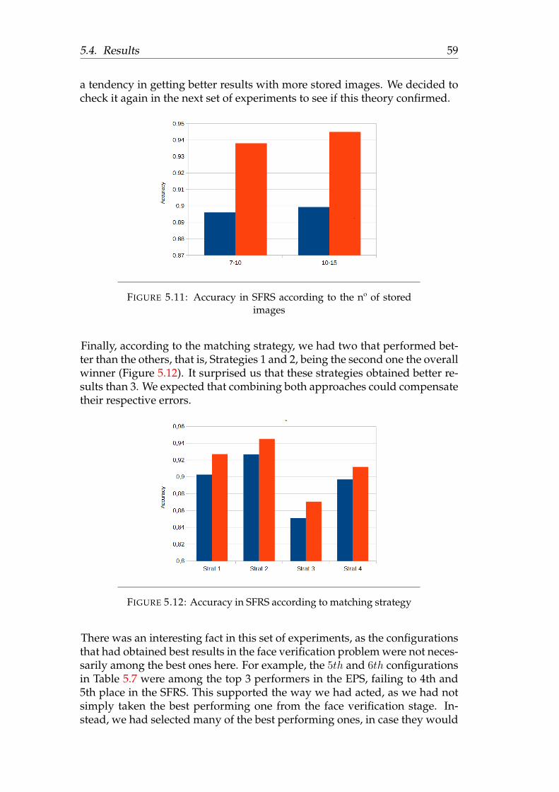
5.4. Results 59
a tendency in getting better results with more stored images. We decided tocheck it again in the next set of experiments to see if this theory confirmed.
FIGURE 5.11: Accuracy in SFRS according to the nº of storedimages
Finally, according to the matching strategy, we had two that performed bet-ter than the others, that is, Strategies 1 and 2, being the second one the overallwinner (Figure 5.12). It surprised us that these strategies obtained better re-sults than 3. We expected that combining both approaches could compensatetheir respective errors.
FIGURE 5.12: Accuracy in SFRS according to matching strategy
There was an interesting fact in this set of experiments, as the configurationsthat had obtained best results in the face verification problem were not neces-sarily among the best ones here. For example, the 5th and 6th configurationsin Table 5.7 were among the top 3 performers in the EPS, failing to 4th and5th place in the SFRS. This supported the way we had acted, as we had notsimply taken the best performing one from the face verification stage. In-stead, we had selected many of the best performing ones, in case they would

60 Chapter 5. Experiments and Results
behave slightly different in the face recognition problem− as it actually hap-pened. That being said, it is true that there was a certain relation betweenboth of them.
Expanded Face Recognition Set
In the last set of experiments, we just tested the 3 best similarity measures,and the results we would consider the obtained results as the definitive facerecognition performance. This time each person would have 30 training im-ages and 50 testing ones, and the number of available people would be morealmost three times as many as in the SFRS. In Table 5.8 we provide the bestresult from all matching strategies −which are later reviewed.
CNN dataset Dropout rate Distance metric Nº images Max Accuracy
Original 0.5 Euclidean 7− 10 0.942Augmented 0.5 Taxicab 7− 10 0.937Augmented 0.5 Euclidean 7− 10 0.937
Original 0.5 Euclidean 10− 15 0.950Augmented 0.5 Taxicab 10− 15 0.945Augmented 0.5 Euclidean 10− 15 0.944
TABLE 5.8: Results EFRS
Surprisingly, we got even better results in this final test, reaching a respectable95% with one of them. Taking into account that it was a more difficult prob-lem, having more people from which to search, we had expected to haveslightly worse results. Even more, due to the lower ethnicity variety, mostindividuals were white people. As they are closer between them, it madethe problem ever harder. However, this dataset provided more training im-ages each person, covering a wider variety of face situations. Therefore,we reached the conclusion that the learning mechanism of the GS had beenable to properly discriminate which images to store. When we checked theamount of images stored per person, in most cases they were higher thanthe required minimum, reaching the maximum allowed in many cases. Ac-cordingly, we achieved better results using any configurations that allowedkeeping a larger number of images than with the other ones (Figure 5.13).
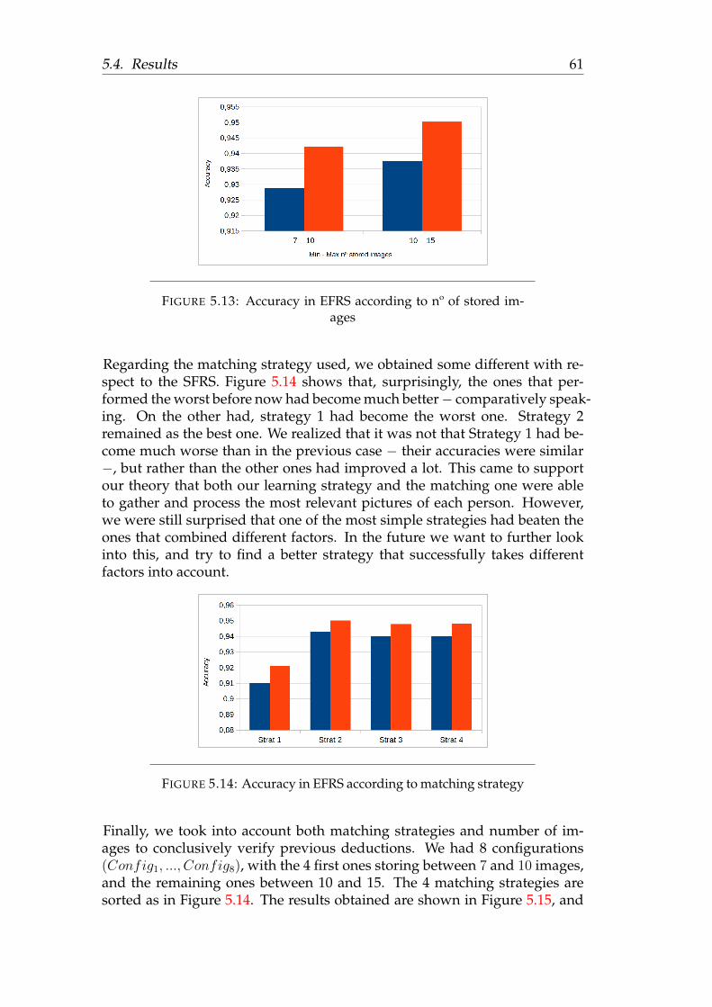
5.4. Results 61
FIGURE 5.13: Accuracy in EFRS according to nº of stored im-ages
Regarding the matching strategy used, we obtained some different with re-spect to the SFRS. Figure 5.14 shows that, surprisingly, the ones that per-formed the worst before now had become much better− comparatively speak-ing. On the other had, strategy 1 had become the worst one. Strategy 2remained as the best one. We realized that it was not that Strategy 1 had be-come much worse than in the previous case − their accuracies were similar−, but rather than the other ones had improved a lot. This came to supportour theory that both our learning strategy and the matching one were ableto gather and process the most relevant pictures of each person. However,we were still surprised that one of the most simple strategies had beaten theones that combined different factors. In the future we want to further lookinto this, and try to find a better strategy that successfully takes differentfactors into account.
FIGURE 5.14: Accuracy in EFRS according to matching strategy
Finally, we took into account both matching strategies and number of im-ages to conclusively verify previous deductions. We had 8 configurations(Config1, ..., Config8), with the 4 first ones storing between 7 and 10 images,and the remaining ones between 10 and 15. The 4 matching strategies aresorted as in Figure 5.14. The results obtained are shown in Figure 5.15, and
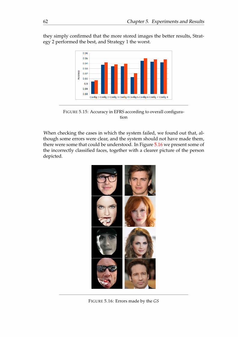
62 Chapter 5. Experiments and Results
they simply confirmed that the more stored images the better results, Strat-egy 2 performed the best, and Strategy 1 the worst.
FIGURE 5.15: Accuracy in EFRS according to overall configura-tion
When checking the cases in which the system failed, we found out that, al-though some errors were clear, and the system should not have made them,there were some that could be understood. In Figure 5.16 we present some ofthe incorrectly classified faces, together with a clearer picture of the persondepicted.
FIGURE 5.16: Errors made by the GS

5.4. Results 63
As it can be seen, they are difficult cases due to different factors. Some ofthem, mainly the first and the third one, could be recognized by a human,but they are more difficult for a machine. On the other hand, the remainingtwo would be actually really difficult, or even impossible, for most humans.There were also other cases we did not expect it to fail, but many of the errorshad some problematic in them. Therefore, this makes the obtained resultseven more worthy, as there were some cases that should be deemed “impos-sible”. However, it remains as a pending task to improve GS in order to beable to properly classify the remaining ones.
To conclude, the best GS achieved a 95% accuracy in the face recognitionproblem, considering 100 people. We consider this result to be a robust one,as there was not a big difference between the configurations, which meantthat it was not simply due to a coincidence. On top of that, the dataset wasreasonably complex, with many people, and a lot of images to test for eachone. Regarding the GS, the learning strategy implemented has proved to beuseful, as the more training images the better results. We also want to allowsystems to keep more than 15 images, and see how they behave. On the otherhand, we have tested different matching strategies, and we have found onethat steadily provides good results, but we still want to try new ones to see ifwe can improve results.


65
Chapter 6
Conclusions
We have developed a fully working Face Recognition system, with the ca-pacity of on-line learning without human intervention. It can work with anykind of images, and is reasonably robust to changes in face expression ororientation, light conditions and other factors. We have based our face ver-ification step on the DeepFace[Taigman et al., 2014] system, which we haveused to provide facial features to our FR system.
The obtained system has been extensively tested, and different parameterscombinations have been tried. We have used the Large Face in the Wild Huanget al., 2007 dataset to assess the performance of our face verification step.Apart from that, we have gathered a 600,000 face images dataset to use bothin training and testing. The facial recognition part has been tested using twodifferent sized datasets, and we have obtained steady results around the 90%of accuracy, reaching a maximum of 95%. These results are better than theones we expected, and they allow for some real life use cases. However,there is still room for improvement, as explained in following Section 6.1.
Two real applications of the FR technology have also been presented. Thefirst one is an online web tool that allows for easily training and testing awhole FR system by simply providing sets of images. Even though it is stillan alpha version, with limited functionality, it is fully operational and hasproven to be useful for demonstration purposes. The other application con-sists in recognizing people in videos. After processing the video, it draws thebounding box of each person in it, following them around the screen, andwrites the name of identified people. It is already working for videos withone person in it, and it is currently being upgraded to allow for multiplepeople recognition.
6.1 Future Work
Throughout the document we have already pointed out some aspects thatshould be improved in the future. The main part that needs to be workedon is to enhance the feature extraction part. The currently used CNNs is stillunderperforming compared with the current state of art. As this part is thebasis of the whole FR system, any improvement made on it will benefit the
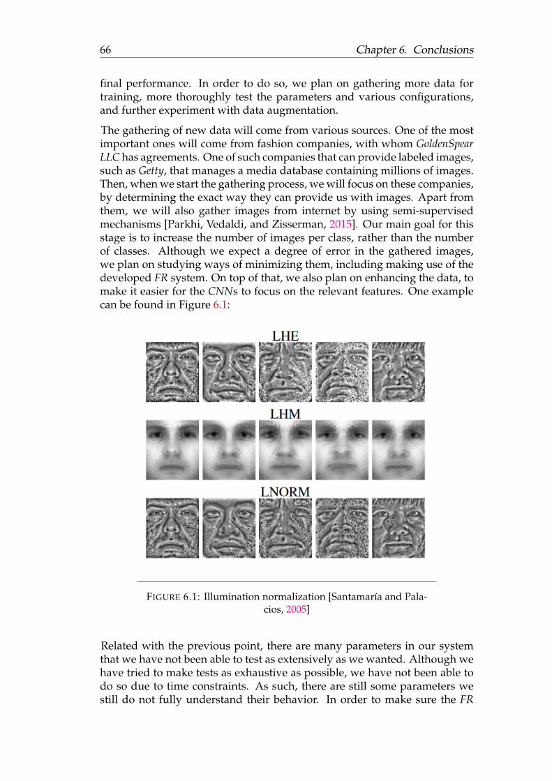
66 Chapter 6. Conclusions
final performance. In order to do so, we plan on gathering more data fortraining, more thoroughly test the parameters and various configurations,and further experiment with data augmentation.
The gathering of new data will come from various sources. One of the mostimportant ones will come from fashion companies, with whom GoldenSpearLLC has agreements. One of such companies that can provide labeled images,such as Getty, that manages a media database containing millions of images.Then, when we start the gathering process, we will focus on these companies,by determining the exact way they can provide us with images. Apart fromthem, we will also gather images from internet by using semi-supervisedmechanisms [Parkhi, Vedaldi, and Zisserman, 2015]. Our main goal for thisstage is to increase the number of images per class, rather than the numberof classes. Although we expect a degree of error in the gathered images,we plan on studying ways of minimizing them, including making use of thedeveloped FR system. On top of that, we also plan on enhancing the data, tomake it easier for the CNNs to focus on the relevant features. One examplecan be found in Figure 6.1:
FIGURE 6.1: Illumination normalization [Santamaría and Pala-cios, 2005]
Related with the previous point, there are many parameters in our systemthat we have not been able to test as extensively as we wanted. Although wehave tried to make tests as exhaustive as possible, we have not been able todo so due to time constraints. As such, there are still some parameters westill do not fully understand their behavior. In order to make sure the FR

6.1. Future Work 67
system is working at full potential, we need to find the optimal parameterconfiguration by means of further testing.
Finally, regarding the two presented applications, as it has already been said,they are not yet completed. We plan on keep working on them so that theweb tool provides more features. And, on the other hand, the video recog-nition part will have to recognize multiple people at once. After that, thereare many further applications in which the FR system can be used, so thereis still lot of work to do with this project.


69
Appendix A
List of names in datasets
A.1 Web Tool
The following ones are the people recognized by the Web Tool:
• Anne Hathaway
• Barack Obama
• Beyonce
• Brad Pitt
• Chiwetel Ejiofor
• Cristiano Ronaldo
• Donald Trump
• Emma Watson
• George Clooney
• Halle Berry
• Hillary Clinton
• Justin Bieber
• Justin Timberlake
• Kate Perry
• Leo Messi
• Madonna
• Morgan Freeman
• Rihanna
• Taylor Swift
• Will Smith

70 Appendix A. List of names in datasets
A.2 Small Face Recognition
The following ones are the people included in the Small Face Recognitiondataset generated by us:
• Aimee Garcia
• Amy Sedaris
• Analeigh Tipton
• Andie MacDowell
• Anton Yelchin
• Arnold Vosloo
• Aziz Ansari
• Barbara Carrera
• Ben Foster
• Blake Lively
• Brad Garrett
• Breckin Meyer
• Brooke Langton
• Cameron Monaghan
• Candace Cameron Bure
• Cedric the Entertainer
• Chiwetel Ejiofor
• Chris Brown
• Claire Holt
• Danay Garcia
• M. Night Shyamalan
• Maksim Chmerkovskiy
• Margaret Cho
• Ming-Na Wen
• Ne-Yo
• Neil deGrasse Tyson
• Omarion Grandberry
• Oprah Winfrey

A.3. Expanded Face Recognition 71
• Reshma Shetty
• Rinko Kikuchi
• Ron Yuan
• Xiao Sun
• Yun-Fat Chow
• Ziyi Zhang
A.3 Expanded Face Recognition
The following ones are the people included in the Expanded Face Recognitiondataset generated by us:
• Alyssa Milano
• Amanda Seyfried
• America Ferrera
• Amy Adams
• Amy Poehler
• Angie Harmon
• Anna Paquin
• Anne Hathaway
• Ashley Benson
• Ben Stiller
• Blake Lively
• Bradley Cooper
• Bryan Cranston
• Christina Hendricks
• Clive Owen
• Colin Firth
• Dana Delany
• Daniel Craig
• David Boreanaz
• David Duchovny
• Diane Kruger

72 Appendix A. List of names in datasets
• Elizabeth Banks
• Emile Hirsch
• Emily Blunt
• Emily Deschanel
• Emma Stone
• Eva Longoria
• Ginnifer Goodwin
• Glenn Close
• Hayden Christensen
• Helen Hunt
• Hilary Swank
• Hugh Jackman
• Jack Black
• Jamie Foxx
• January Jones
• Jared Padalecki
• Jason Bateman
• Jennifer Lawrence
• Jeremy Renner
• Jessica Chastain
• Jim Parsons
• John Krasinski
• Jon Hamm
• Jonah Hill
• Joseph Gordon-Levitt
• Josh Brolin
• Josh Duhamel
• Joshua Jackson
• Julia Louis-Dreyfus
• Julia Roberts
• Julie Benz
• Julie Bowen

A.3. Expanded Face Recognition 73
• Kaley Cuoco
• Kate Beckinsale
• Kate Bosworth
• Kate Walsh
• Katherine Heigl
• Kellan Lutz
• Kevin Bacon
• Kirstie Alley
• Kristen Bell
• Kristen Stewart
• Lea Michele
• Leighton Meester
• Liev Schreiber
• Lisa Kudrow
• Luke Wilson
• Marcia Cross
• Marion Cotillard
• Mark Ruffalo
• Mich
• Michael Weatherly
• Michelle Trachtenberg
• Michelle Williams
• Mila Kunis
• Miley Cyrus
• Natalie Portman
• Nathan Fillion
• Neil Patrick Harris
• Olivia Wilde
• Paul Rudd
• Quentin Tarantino
• Robert Pattinson
• Ryan Reynolds

74 Appendix A. List of names in datasets
• Sarah Hyland
• Scarlett Johansson
• Selena Gomez
• Simon Baker
• Simon Pegg
• Sofia Vergara
• Stana Katic
• Steve Carell
• Summer Glau
• Taylor Swift
• Teri Hatcher
• Terrence Howard
• Vanessa Hudgens
• Zac Efron
• Zooey Deschanel

75
Bibliography
Aarts, Emile and Jan Korst (1989). Simulated Annealing and Boltzmann Ma-chines: A Stochastic Approach to Combinatorial Optimization and Neural Com-puting. New York, NY, USA: John Wiley & Sons, Inc. ISBN: 0-471-92146-7.
Abadi, Martín et al. (2016). “TensorFlow: A system for large-scale machinelearning”. In: CoRR abs/1605.08695. URL: http://arxiv.org/abs/1605.08695.
Belhumeur, P. N. et al. (2011). “Localizing Parts of Faces Using a Consensus ofExemplars”. In: Proceedings of the 2011 IEEE Conference on Computer Visionand Pattern Recognition. CVPR ’11. Washington, DC, USA: IEEE ComputerSociety, pp. 545–552. ISBN: 978-1-4577-0394-2. DOI: 10 . 1109 / CVPR .2011.5995602. URL: http://dx.doi.org/10.1109/CVPR.2011.5995602.
Berg, Thomas and Peter N. Belhumeur (2012). “Tom-vs-Pete Classifiers andIdentity-Preserving Alignment for Face Verification”. In: BMVC.
Cao, Xudong et al. (2013). “A Practical Transfer Learning Algorithm for FaceVerification”. In: Proceedings of the 2013 IEEE International Conference onComputer Vision. ICCV ’13. Washington, DC, USA: IEEE Computer Soci-ety, pp. 3208–3215. ISBN: 978-1-4799-2840-8. DOI: 10.1109/ICCV.2013.398. URL: http://dx.doi.org/10.1109/ICCV.2013.398.
Chellappa, R., C.L. Wilson, and S. Sirohey (1995). “Human and machine recog-nition of faces: a survey”. In: Proceedings of the IEEE 85.5, pp. 705 –741.ISSN: 1558-2256. DOI: 10.1109/5.381842. URL: https://engineering.purdue.edu/~ece624/papers/challapa_facerecognition.pdf.
Chen, Bor-Chun, Chu-Song Chen, and Winston H. Hsu (2014). “Cross-AgeReference Coding for Age-Invariant Face Recognition and Retrieval”. In:Proceedings of the European Conference on Computer Vision (ECCV).
Chen, Dong et al. (2012). “Bayesian Face Revisited: A Joint Formulation”. In:Proceedings of the 12th European Conference on Computer Vision - Volume PartIII. ECCV’12. Florence, Italy: Springer-Verlag, pp. 566–579. ISBN: 978-3-642-33711-6. DOI: 10.1007/978-3-642-33712-3_41. URL: http://dx.doi.org/10.1007/978-3-642-33712-3_41.
Chen, Dong et al. (2013). “Blessing of Dimensionality: High-DimensionalFeature and Its Efficient Compression for Face Verification”. In: Proceed-ings of the 2013 IEEE Conference on Computer Vision and Pattern Recognition.CVPR ’13. Washington, DC, USA: IEEE Computer Society, pp. 3025–3032.ISBN: 978-0-7695-4989-7. DOI: 10.1109/CVPR.2013.389. URL: http://dx.doi.org/10.1109/CVPR.2013.389.
76 BIBLIOGRAPHY
Cho, Youngmin and Lawrence K Saul (2009). “Kernel methods for deep learn-ing”. In: Advances in neural information processing systems, pp. 342–350.
Chollet, François (2015). Keras. https://github.com/fchollet/keras.Cootes, Tim. “An introduction to active shape models”. In:Deco, Gustavo and Tai Sing Lee (2004). “The role of early visual cortex in
visual integration: a neural model of recurrent interaction”. In: EuropeanJournal of Neuroscience 20.4, pp. 1089–1100. ISSN: 1460-9568. DOI: 10.1111/j.1460-9568.2004.03528.x. URL: http://dx.doi.org/10.1111/j.1460-9568.2004.03528.x.
DeepMind (2016). Publications | Deepmind. https :/ / deepmind. com/research/publications/. [Online; accessed 13/1/2017].
Goodfellow, Ian, Yoshua Bengio, and Aaron Courville (2016). Deep Learning.http://www.deeplearningbook.org. MIT Press.
Goodfellow, Ian J. et al. (2013). “Pylearn2: a machine learning research li-brary”. In: arXiv preprint arXiv:1308.4214. URL: http://arxiv.org/abs/1308.4214.
Haghighat, Mohammad (2016). Gabor Feature Extraction. https : / / es .mathworks.com/matlabcentral/fileexchange/44630-gabor-feature-extraction. [Online; accessed 12/1/2017].
Hassner, Tal et al. (2015). “Effective Face Frontalization in Unconstrained Im-ages”. In: IEEE Conf. on Computer Vision and Pattern Recognition (CVPR).URL: \urlhttp://www.openu.ac.il/home/hassner/projects/frontalize.
He, Xiaofei et al. (2005). “Face recognition using Laplacianfaces”. In: IEEEtransactions on pattern analysis and machine intelligence 27.3, pp. 328–340.
Hinton, Geoffrey E, Simon Osindero, and Yee-Whye Teh (2006). “A fast learn-ing algorithm for deep belief nets”. In: Neural computation 18.7, pp. 1527–1554.
Huang, Gary B. et al. (2007). Labeled Faces in the Wild: A Database for StudyingFace Recognition in Unconstrained Environments. Tech. rep. 07-49. Univer-sity of Massachusetts, Amherst.
Itti, Laurent and Christof Koch (2001). “Computational Modelling of VisualAttention”. In: Nature Reviews Neuroscience 2.3, pp. 194–203. ISSN: 1471-003X. DOI: 10.1038/35058500. URL: \urlhttp://www.nature.com/nrn/journal/v2/n3/full/nrn0301_194a.html.
Kelly, Michael David (1971). “Visual Identification of People by Computer”.AAI7112934. PhD thesis. Stanford, CA, USA.
Kim, Jonghong, Seonggyu Kim, and Minho Lee (2015). “Convolutional Neu-ral Network with Biologically Inspired ON/OFF ReLU”. In: Neural In-formation Processing: 22nd International Conference, ICONIP 2015, November9-12, 2015, Proceedings, Part IV. Ed. by Sabri Arik et al. Cham: SpringerInternational Publishing, pp. 316–323. ISBN: 978-3-319-26561-2. DOI: 10.1007/978-3-319-26561-2_38. URL: http://dx.doi.org/10.1007/978-3-319-26561-2_38.
Lee, Honglak et al. (2011). “Unsupervised learning of hierarchical represen-tations with convolutional deep belief networks”. In: Communications ofthe ACM 54.10, pp. 95–103.

BIBLIOGRAPHY 77
Liu, Chengjun and H. Wechsler (2002). “Gabor Feature Based ClassificationUsing the Enhanced Fisher Linear Discriminant Model for Face Recog-nition”. In: Trans. Img. Proc. 11.4, pp. 467–476. ISSN: 1057-7149. DOI: 10.1109/TIP.2002.999679. URL: http://dx.doi.org/10.1109/TIP.2002.999679.
Lyons, M. et al. (1998a). “Coding Facial Expressions with Gabor Wavelets”.In: Proceedings of the 3rd. International Conference on Face & Gesture Recog-nition. FG ’98. Washington, DC, USA: IEEE Computer Society, pp. 200–.ISBN: 0-8186-8344-9. URL: http://dl.acm.org/citation.cfm?id=520809.796143.
— (1998b). “Coding Facial Expressions with Gabor Wavelets”. In: Proceedingsof the 3rd. International Conference on Face & Gesture Recognition. FG ’98.Washington, DC, USA: IEEE Computer Society, pp. 200–. ISBN: 0-8186-8344-9. URL: http://dl.acm.org/citation.cfm?id=520809.796143.
Montana, David J. and Lawrence Davis (1989). “Training Feedforward Neu-ral Networks Using Genetic Algorithms”. In: Proceedings of the 11th In-ternational Joint Conference on Artificial Intelligence - Volume 1. IJCAI’89.Detroit, Michigan: Morgan Kaufmann Publishers Inc., pp. 762–767. URL:http://dl.acm.org/citation.cfm?id=1623755.1623876.
Ng, Hongwei and Stefan Winkler (2014). “A data-driven approach to clean-ing large face datasets”. In: ICIP.
Parkhi, Omkar M, Andrea Vedaldi, and Andrew Zisserman (2015). “Deepface recognition”. In: British Machine Vision Conference. Vol. 1. 3, p. 6.
Pham, Dung Viet (2012). “Online handwriting recognition using multi con-volution neural networks”. In: Asia-Pacific Conference on Simulated Evolu-tion and Learning. Springer, pp. 310–319.
Ren, Shaoqing et al. (2015). “Faster R-CNN: Towards Real-Time Object De-tection with Region Proposal Networks”. In: Advances in Neural Informa-tion Processing Systems 28. Ed. by C. Cortes et al. Curran Associates, Inc.,pp. 91–99. URL: http://papers.nips.cc/paper/5638-faster-r-cnn-towards-real-time-object-detection-with-region-proposal-networks.pdf.
Salah, Albert Ali et al. (2007). “Hidden Markov model-based face recognitionusing selective attention”. In: Human Vision and Electronic Imaging XII, SanJose, CA, USA, January 29 - February 1, 2007, p. 649214. DOI: 10.1117/12.707333. URL: http://dx.doi.org/10.1117/12.707333.
Santamaría, Mauricio Villegas and Roberto Paredes Palacios (2005). “Com-parison of illumination normalization methods for face recognition”. In:
Schroff, Florian, Dmitry Kalenichenko, and James Philbin (2015). “FaceNet:A Unified Embedding for Face Recognition and Clustering”. In: CoRRabs/1503.03832. URL: http://arxiv.org/abs/1503.03832.
Serra, Xavier (2016). Face Recognition APP. http://app.goldenspear.com/tools/face_recognition/face_recognition.html. [On-line; accessed 16/1/2017].

78 BIBLIOGRAPHY
Taigman, Yaniv et al. (2014). “DeepFace: Closing the Gap to Human-LevelPerformance in Face Verification”. In: Proceedings of the 2014 IEEE Confer-ence on Computer Vision and Pattern Recognition. CVPR ’14. Washington,DC, USA: IEEE Computer Society, pp. 1701–1708. ISBN: 978-1-4799-5118-5. DOI: 10.1109/CVPR.2014.220. URL: http://dx.doi.org/10.1109/CVPR.2014.220.
Turk, Matthew and Alex Pentland (1991). “Eigenfaces for Recognition”. In:J. Cognitive Neuroscience 3.1, pp. 71–86. ISSN: 0898-929X. DOI: 10.1162/jocn.1991.3.1.71. URL: http://dx.doi.org/10.1162/jocn.1991.3.1.71.
Utsav Prabhu and Keshav Seshadri (2009). http://www.contrib.andrew.cmu.edu/~kseshadr/ML_Paper.pdf. [Online, accessed on 15-December-2016].
Wiskott, Laurenz et al. (1997). “Face Recognition by Elastic Bunch GraphMatching”. In: IEEE Trans. Pattern Anal. Mach. Intell. 19.7, pp. 775–779.ISSN: 0162-8828. DOI: 10.1109/34.598235. URL: http://dx.doi.org/10.1109/34.598235.
Yamazaki, A., M.C.P. de Souto, and T.B. Ludermir (2002). “Optimization ofneural network weights and architectures for odor recognition using sim-ulated annealing”. In: International Joint Conference on Neural Networks.IJCNN’02. IEEE. ISBN: 0-7803-7278-6. DOI: 10 . 1109 / IJCNN . 2002 .1005531. URL: http://ieeexplore.ieee.org/document/1005531/.
Yi, Dong et al. (2014). “Learning Face Representation from Scratch”. In: CoRRabs/1411.7923. URL: http://arxiv.org/abs/1411.7923.