Face Recognition Using

Different Training Data

By

LI Zhifeng

A Thesis Submitted in Partial Fulfillment

of the Requirements for the Degree of

Master of Philosophy

in

Information Engineering

• The Chinese University of Hong Kong

December 2002

The Chinese University of Hong Kong holds the copyright of this thesis. Any

person(s) intending to use a part or whole of the materials in the thesis in a

proposed publication must seek copyright release from the Dean of the Graduate

School.

r 2 8 P • m

UNIVERSITY /r5��/ \ 5cNaiSRAfiY SYSTEM

Abstract Face recognition is one of the most challenging computer vision research topics

since faces appear differently even for the same person due to expression, pose,

lighting, occlusion and many other confounding factors in real life. During the

past thirty years, a number of face recognition techniques have been proposed. In

general, these methods can be divided into two categories: "appearance-based"

and "feature-based". For appearance-based methods, holistic features are

extracted from the face images and then used for classification. For feature-based

method, local and geometrical features are extracted from the face images and

used for classification. R. Brunelli and T. Poggio have conducted the comparative

research about the above two categories and pointed out that appearance-based

methods outperform the feature-based methods. Therefore in this thesis I focus on

the study of appearance-based methods.

Generally, the procedure of appearance-based methods can be described as the

follows. First, extract the holistic feature vectors from the training data, and then

transform the probe data and the gallery data using these feature vectors. Finally,

classification is performed by comparing the transformed probe data and the

transformed gallery data. The performance of appearance-based methods depends

heavily on the selection of training data since the feature vectors are extracted

directly from the training data. However, until now most researches simply

randomly choose some training samples for computation of the feature vectors

without much justification. In this thesis, we conduct a systematic experimental

study on the relationship between the appearance-based methods and different

training data. Principal Component Analysis (PCA) and Linear discriminant

Analysis (LDA) are the two most representative techniques in Appearance-based

methods. The former is optimal for face representation and the latter is effective

for face classification. Many face recognition methods proposed in recent years

are related to PCA or LDA techniques. Therefore in this thesis I select these two

techniques for comparative study. For evaluation of the performance of different

training data, we use three face databases: XM2VTS face database, AR face

database (Purdue University), and MMLAB face database.

i

Experimental results show that simply increasing the number of training

samples for each person does not help to improve the recognition performance for

both the two methods. For PCA-based method, increasing the number of people

benefits the recognition performance more than increasing the number of face

images per person. For LDA-based method, the recognition performance depends

more on the mixture of the right variety of images in the training data than on the

size of the training data.

This work will benefit the improvement of face recognition performance and

efficacy by choosing appropriate training data. Especially it may benefit the

research on face recognition in video where large amount of face images are

involved.

ii

摘要

人像識別是最富有挑戰性的計算機視覺硏究課題之一，因爲

即使是相同的人在不同的表情，姿勢，光線，遮掩物及其很多其

它現實生活中的干擾因素作用下人像會表現出很大的差異性。在

過去的三十多年裡有很多人像識別技術被提出。總的說來這些技

術可以被分成兩大類：“基于外觀的（appearance-based)”和

“基于特征的（ fea ture-based)”。基于外觀的方法從人像中提

取整體的特征用作識別。基于特征的方法從人像中提取局部和幾

何特征用作識別。R. B r u n e i 1 1 和 T . Poggio曾經對這兩類方法

做過比較性的硏究並指出基于外觀的方法要好與基于特征的方

法。因此在本論文中我主要關注基于外觀的方法。

總的說來基于外觀的方法的流程可以簡述如下：首先從訓練

數據中提取整體性的特征向量然後用這些特征向量來變換檢測圖

像和已知身份的參考人像，最後通過比較監測人像和參考人像變

換后的結果來進行分類。從上述描述中我們可以看出基于外觀的

方法的性能很大程度上依靠訓練數據的選取因爲那些特征向量是

直接從訓練數據中提取出來的。然而至今爲止大多數的硏究者只

是沒有太多理由的簡單地選取一些訓練樣本用于計算這些特征向

量。在本論文中，我們進行了一系列系統性的實驗來硏究基于外

觀的人像識別方法和不同的訓練數據之間的關係。因爲主分量分

析(PCA)和線性判別式分析(LDA)是基于外觀的方法中最富有典型

性和代表性的兩類方法，前者對人像表示而言是最優的後者對人

像分類而言是最優的，大部份近年來提出的人像識別方法都是基

iii

于PCA技術或者是LDA技術，因此在本論文中我們選擇這兩種技

術用于比較性的硏究和評估不同訓練數據的性能，這些訓練數據

選自三個大的人臉數據庫：XM2VTS人臉數據庫，AR人臉數據庫

(Purdue大學），和MMLAB人臉數據庫。

實驗結果顯示對PCA和LDA這兩種方法而言簡單的增加每一

個人的訓練樣本數目不能有助于識別性能的提高。對于基于PCA

的識別方法，增加訓練人數比增加每一個人的訓練樣本數要更有

利于識別性能的提高；對于基于LDA的識別方法，識別性能更多

的依賴于訓練數據中適當的多樣性的圖像的組合而不是訓練樣本

的數量大小。

我們的工作對于硏究如何選取合適的訓練數據以提高人像識

別率和性能有很大的幫助，特別對基于視頻的人像識別硏究有很

大的幫助因爲大量的人像包含在視頻中。

iv

Acknowledgments Here I would like to thank all the persons who have helped me during my

master studies at the Dept. of Information Engineering, The Chinese University of

Hong Kong.

Firstly I would like to thank my supervisor, Prof. Xiaoou Tang, for his zealous

support and guidance on my research work. He is always very friendly and

understanding. I leam many things from him.

Then I would also like to thank my all colleagues in Multimedia Lab, Deft. Of

Information Engineering, Feng Lin, Xiaogang Wang, Bo Luo, Feng Zhao,

Dacheng Tao, Lifeng Sha, Hua Shen, Tong Wang for their zealous help.

Finally I would like to thank my family, especially my parents and my sister for

their support, care and encouragement.

V

Table of Contents

Abstract i

Acknowledgments v

Table of Contents vi

List of Figures viii

List of Tables ix

Chapter 1 Introduction 1

1.1 Face Recognition Problem and Challenge 1 1.2 Applications 2 1.3 Face Recognition Methods 3 1.4 The Relationship Between the Face Recognition Performance and Different

Training Data 5 1.5 Thesis Overview 6

Chapter 2 PCA-based Recognition Method 7

2.1 Review 7 2.2 Formulation 8 2.2.1 Karhunen-Loeve transform (KLT) .8 2.2.2 Multilevel Dominant Eigenvector Estimation (MDEE) 12 2.3 Analysis of The Effect of Training Data on PCA-based Method 13

Chapter 3 LDA-based Recognition Method 17

3.1 Review 17 3.2 Formulation 18 3.2.1 The Pure LDA 18 3.2.2 LDA-based method 19 3.3 Analysis of The Effect of Training Data on LDA-based Method 21

Chapter 4 Experiments 23

4.1 Face Database 23 4.1.1 AR face database 23 4.1.2 XM2VTS face database 24 4.1.3 MMLAB face database 26 4.1.4 Face Data Preprocessing 27 4.2 Recognition Formulation 29 4.3 PCA-based Recognition Using Different Training Data Sets 29 4.3.1 Experiments on MMLAB Face Database 30 4.3.1.1 Training Data Sets and Testing Data Sets 30 4.3.1.2 Face Recognition Performance Using Different Training Data Sets 31 4.3.2 Experiments on XM2VTS Face Database 33 4.3.3 Comparison of MDEE and KLT 36

vi

4.3.4 Summary 38 4.4 LDA-based Recognition Using Different Training Data Sets 38 4.4.1 Experiments on AR Face Database 38 4.4.1.1 The Selection of Training Data and Testing Data 38 4.4.1.2 LDA-based recognition on AR face database 39 4.4.2 Experiments on XM2VTS Face Database 40 4.4.3 Training Data Sets and Testing Data Sets 41 4.4.4 Experiments on XM2VTS Face Database 42 4.4.5 Summary 46

Chapter 5 Summary 47

Bibliography 49

vii

List of Figures Figure 1.1 The procedure of face recognition 1 Figure 1.2 26 face images of one person in the AR face database 2 Figure 2.1 Face space 14 Figure 2.2 Principal component of small number of persons 15 Figure 2.3 Principal component of small number of persons 15 Figure 2.4 Principal component of large number of persons 16 Figure 4.1 Some examples of AR face database 24 Figure 4.2 20 samples captured from one person's video 25 Figure 4.3 Some examples of the XM2VTS face database 25 Figure 4.4 Some examples of MMLAB face database 27 Figure 4.5 20 normalized samples of one person from XM2VTS database. ..28 Figure 4.6 Some normalized samples from MMLAB face database 28 Figure 4.7 Face recognition performance based on the three training subsets

of training data set #1 from MMLAB face database 32 Figure 4.8 Face recognition performance based on the three training subsets

of training data set #1 from XM2VTS database 35 Figure 4.9 (a)-(f): Top 300 eigenvalues ofMDEE and KLT 37 Figure 4.10 Recognition performance of training data set # 1 43 Figure 4.11 Recognition performance of training data set #2 44 Figure 4.12 Recognition performance of training data set #3 45

viii

List of Tables

Table 1.1 Some applications of face recognition [2] 3 Table 4.1 Description of 26 face images of each person from the AR face

database 23 Table 4.2 Description of the ten face videos 26 Table 4.3 Different training data sets from MMLAB face database 30 Table 4.4 Face recognition performance based on the three training subsets of

training data set #1 from MMLAB face database 32 Table 4.5 Face recognition performance based on the three training subsets in

training data set #2 from MMLAB face database 33 Table 4.6 Different training data sets from XM2VTS face database 34 Table 4.7 Face recognition performance based on the three training subsets of

training data set #1 from XM2VTS database 34 Table 4.8 Face recognition performance based on the three training subsets of

training data set #2 from XM2VTS database 35 Table 4.9 Recognition rate comparison of MDEE and KLT 36 Table 4.10 Training data structure 39 Table 4.11 Testing data structure 39 Table 4.12 Recognition accuracy of different training data from Purdue

database 40 Table 4.13 The division scheme of development and sequestered portions. ...41 Table 4.14 Training data set #1 41 Table 4.15 Training data set #2 42 Table 4.16 Training data set #3 42 Table 4.17 Recognition performance of training data set #1 43 Table 4.18 Recognition performance of training data set #2 44 Table 4.19 Recognition performance of training data set #3 45

ix

Chapter 1

Introduction

1.1 Face Recognition Problem and

Challenge Face recognition problem can be described as the follows: given still or video face

images of a reference face database (gallery set) and a probe database (probe set),

identify which person in the gallery set are most similar to the test person in the

probe set. Similar to other pattern recognition problem, face recognition can be

divided into two steps: feature extraction and feature matching. Figure 1.1 shows

the procedure of face recognition.

Feature ^ Feature ^ ‘ ^ Extraction Matching

Test face : _ Test Output feature vector

Reference feature

^ vectors

Reference J F e a t u r e ^ ^ Database ^ , Extract腿

Reierence ^ � faces

Figure 1.1 The procedure of face recognition.

Face recognition is one of the most challenging computer vision research topics

since faces appear differently even for the same person due to expression, pose,

occlusion and many other confounding factors in real life. These variations are

called intra-personal variations or within-class variations since they are for the

same person. Figure 1.2 shows the intra-personal variations of one person from

1

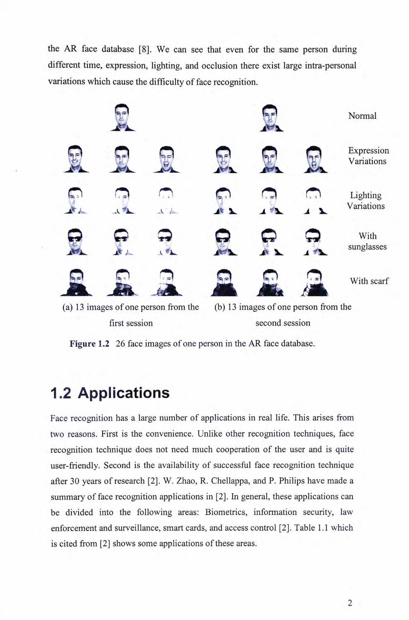
the AR face database [8]. We can see that even for the same person during

different time, expression, lighting, and occlusion there exist large intra-personal

variations which cause the difficulty of face recognition.

^ ^ Normal

Q Q O Q Q Expression ^ ^ ^ ^ ^ Variations

O Q i D O Lighting

丄‘ . 處 丄丄. A a . i l j Variations

9 Q Q Q Q O With ^ ^ Jt；. .人 J ^ J k i l sunglasses

£ £ ^ 息 i 碰 scarf

^^-JBH^ JEUIv,, . ^J^^Bl Mt/KBSL IW^k (a) 13 images of one person from the (b) 13 images of one person from the

first session second session

Figure 1.2 26 face images of one person in the AR face database.

1.2 Applications Face recognition has a large number of applications in real life. This arises from

two reasons. First is the convenience. Unlike other recognition techniques, face

recognition technique does not need much cooperation of the user and is quite

user-friendly. Second is the availability of successful face recognition technique

after 30 years of research [2]. W. Zhao, R. Chellappa, and P. Philips have made a

summary of face recognition applications in [2]. In general, these applications can

be divided into the following areas: Biometrics, information security, law

enforcement and surveillance, smart cards, and access control [2]. Table 1.1 which

is cited from [2] shows some applications of these areas.

2

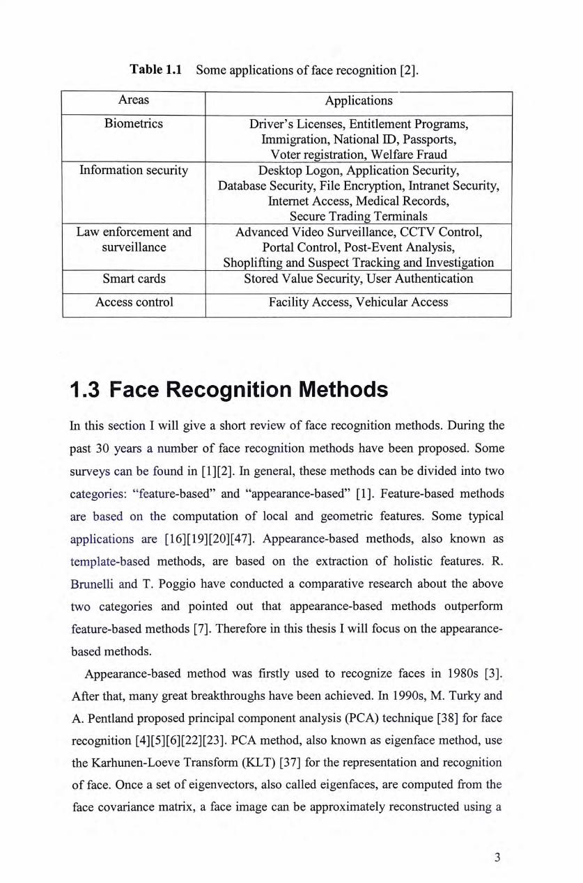
Table 1.1 Some applications of face recognition [2 .

Areas Applications

Biometrics Driver's Licenses, Entitlement Programs, Immigration, National ID, Passports,

Voter registration, Welfare Fraud Information security Desktop Logon, Application Security,

Database Security, File Encryption, Intranet Security, Internet Access, Medical Records,

Secure Trading Terminals Law enforcement and Advanced Video Surveillance, CCTV Control,

surveillance Portal Control, Post-Event Analysis, Shoplifting and Suspect Tracking and Investigation

Smart cards Stored Value Security, User Authentication

Access control Facility Access, Vehicular Access

1.3 Face Recognition Methods In this section I will give a short review of face recognition methods. During the

past 30 years a number of face recognition methods have been proposed. Some

surveys can be found in [1][2]. In general, these methods can be divided into two

categories: "feature-based" and "appearance-based" [1]. Feature-based methods

are based on the computation of local and geometric features. Some typical

applications are [16] [19] [20] [47]. Appearance-based methods, also known as

template-based methods, are based on the extraction of holistic features. R.

Brunelli and T. Poggio have conducted a comparative research about the above

two categories and pointed out that appearance-based methods outperform

feature-based methods [7]. Therefore in this thesis I will focus on the appearance-

based methods.

Appearance-based method was firstly used to recognize faces in 1980s [3'.

After that, many great breakthroughs have been achieved. In 1990s, M. Turky and

A. Pentland proposed principal component analysis (PCA) technique [38] for face

recognition [4] [5] [6] [22] [23]. PC A method, also known as eigenface method, use

the Karhunen-Loeve Transform (KLT) [37] for the representation and recognition

of face. Once a set of eigenvectors, also called eigenfaces, are computed from the

face covariance matrix, a face image can be approximately reconstructed using a

3

weighted combination of the eigenfaces. The weights that characterize the

expansion of the given image in terms of eigenfaces constitute the feature vector.

When a new test image is given, the weights are computed by projecting the

image onto the eigenface vectors. The classification is then carried out by

comparing the distances between the weight vectors of the test image and the

weight vectors of the images from the database. Eigenface method takes

advantage of the structure similarity of faces and produces a highly compressed

representation of face, thus greatly improve the face recognition efficiency. This

method, after proposed in early 1990s, has quickly become one of the most

popular face recognition techniques [1]. Although PCA method achieves great

success in face recognition, it still has some limitations. In recent years

researchers proposed the Linear Discriminating Analysis (LDA) technique for

face recognition [9][10][11][12][35][43]. LDA method, which is based on Fisher

Linear Discriminant (FLD) [13]，can discriminate the intra-personal variations

(caused during the same person, also called within-class variations) and extra-

personal variations (caused by different persons, also called between-class

variations). This method seeks to find the most discriminating features which

maximize the ratio between the between-class variations and within-class

variations [9:.

Until now people have proposed a number of appearance-based face

recognition techniques, among which PCA technique and LDA technique are

among the most popular and representative ones. Some evaluation study of these

two techniques can be found in [21] [26] [31]. In Face Recognition Technology

(FERET) test [49][50][51], these two techniques are among the most successful

ones. In recent years quite a few new face recognition techniques are proposed

and most of them are still related to these two techniques. Therefore in this thesis I

select these two methods for comparative study and evaluation the performance of

different training data.

4

1.4 The Relationship Between the Face

Recognition Performance and

Different Training Data For appearance-based face recognition methods, since the feature vectors for

classification are all computed directly from the training data, it is reasonable to

expect that the recognition results may be influenced by different training data

sets. However, until now, most previous researches only simply choose a small

number of training samples randomly to compute features without much

justification. In this thesis, I will explore this meaningful and important topic.

It is generally believed that increasing the size of training data will benefit the

recognition performance. In this thesis I will show that is not always the case. I

select two representative techniques: PCA and LDA to explore the relationship

between the face recognition performance and different training data. Theoritical

analysis and experimental results show that size of the training data is not the

critical factor. For PCA-based method, increasing the number of persons appeared

in the training data benefit the recognition performance more than increasing the

number of images per person. For LDA-based method, we found that simply

increasing the number of samples per person from the same session will not

benefit the recognition performance. The important factor is not the size of the

training data, rather is the variety of the training data. By selecting the training

data from different sessions, we can capture the intra-personal variations that

exists between the probe set and gallery set, thus give much better recognition

performance.

In this thesis, we will first review the PCA method and LDA method and then

analyze the affect of the training data on face recognition performance. Finally we

confirm our analysis using a systematic experimental study.

»

5

1.5 Thesis Overview The rest of this thesis is organized as follows. Chapter 2 gives the review on PCA

method and analyzes the effect of training data on the PCA method. Chapter 3

gives the review on LDA method and analyzes the effect of training data on this

method. Chapter 4 shows the experimental results and analysis. Chapter 5 is the

summary.

6

Chapter 2

PCA-based Recognition Method

2.1 Review Principal Component Analysis (PCA) method, also known as eigenface method, is

based on Karhunen-Loeve transform (KLT). In 1990 Kriby and Sirovich first use

it to characterize faces [14]. Later, in 1991，Turk and Pentland proposed eigenface

method based on it [4] [5]. In eigenface method, a 2-dimensional N by M face

image is represented by a one-dimensional face vector with the length n = N*M.

Then we calculate the eigenvectors of the covariance matrix of all the training

face vectors. Once a set of eigenvectors, also called eigenfaces, is computed from

the face covariance matrix, a face image can be approximately reconstructed using

a weighted combination of the eigenfaces. The weights that characterize the

expansion of the given image in terms of eigenfaces constitute the feature vector.

When a new test image is given, the weights are computed by projecting the

image onto the eigenface vectors. The classification is then carried out by

comparing the distances between the weight vectors of the test image and the

images from the database. Eigenface method can extract the most expressive

features while remove the redundancy components of the raw face as much as

possible. It can lower the dimension of the face vector drastically while keep up

most of useful information. Note that all faces look like each other since they all

have two eyes, one nose, one mouth, two ears, and so on [52]. In other words,

they have the similarity of the structure. This implies the fact that the raw face

vector contains a great amount of redundancy. Using the raw face vector for

classification need much computation since the dimension of face vector is always

very large. Eigenface method uses this property of faces to reduce the redundancy

components as much as possible. After it was proposed in 1991, this method has

become one of the most popular face recognition methods [1]. Although eigenface

method is effective and easy to apply, it is not robust, especially compared with

7

LDA-based method. Eigenface method performs well under strictly controlled

conditions but tend to suffer under uncontrained conditions. To improve the

robustness of the PC A method, in 1994，A. Pentland, B. Moghaddam and T.

Stamer proposed the view-based and modular eigenspaces method for face

recognition [6]. They improve PCA method by using view-based eigenface to

handle the change of pose, and use modular eigenfeatures, e.g. eigeneyes,

eigennose, eigenmouth, instead of the coarse eigenface, to improve the robustness

:6]. In 1997 and 1998, B. Moghaddam and A. Pentland further improve the

eigenface method by proposing probabilistic visual learning and Bayes matching

techniques [22] [23]. In recent years, researchers proposed many other new PCA-

related face recognition methods and achieve great success, including method that

combine PCA and Kernel function [32], methods that combine PCA and Bayes

matching [31][52]，and method that combine PCA and Gabor filter [36'.

2.2 Formulation The eigenface method is based on Karhunen-Loeve transform (KLT). Kirby and

Sirovich first use eigenfaces to characterize faces [14]. Later, Turk and Pentland

apply the approach on face recognition [4][5]. We now briefly review the basic

idea of the eigenface method.

2.2.1 Karhunen-Loeve transform (KLT)

Letxj ... x’m represent a set of n-dimension random vectors and fi is the mean

vector. The procedure of computing the Karhunen-Loeve transform is described

as the follows:

(1) Form the nhym sample matrix

�1(1) ... xM

h x�(2)义2(2) ... x„{2)， （2.1)

x^{n) ... x„{n)_

where x. = x , i s the length of each vector, and m is the number of vectors.

8

(2) Estimate the covariance matrix,

/ m 1

W = - y x , x f = - A A ' . (2.2) m ^ m

(3) Compute the eigenvectors of the covariance matrix and select k eigenvectors

F,厂2 ... k with the largest eigenvalues to form the transform matrix,

B = [V丨 V, ... V J . (2.3)

(4) For a new ^-dimension vector x, we project it in the subspace spanned by the k

eigenvectors,

y = B T ( x i ) , (2.4)

where y is the weight vector that characterizes the projection of the vector x in the

subspace supported by the k eigenvectors.

The most prominent advantage of KLT is that it can reduce the correlation and

cluster information as much as possible. It is optimal for reconstruction and

compression under minimum mean-square error.

Given a random vector x with dimension n, we would like to approximate it

using a linear combination of k vectors from n orthonormal basis ( e � i 二 1,2,...,

n) .

The linear reconstruction of x using k vectors can be described as, , k

= (2.5) i=l

where c. is the coefficients.

Since the dimension of x is n and there are n orthonormal basis. Therefore x

can be expressed by, n

(2.6) i=l

The error of reconstruction is n

d =x-x = Yj^iCi (2.7) i=k+l

We would like to choose the optimal basis such that the mean-square error A is

minimized.

^ - E(\d\') = E(d'd) = E(( Y CiC^X = E( f^c；) (2.8) i=k+I i=k+l i=k+l

Note that

9

c =efx = x^e- (2.9)

Then

zl= X E ( c ” = (2.10) i=k+J i=k+l i=k+l

Let

W = E(xx^) (2.11)

Where W is the covariance matrix of the random vector x.

We have

YeJWe, (2.12) i=k+l

Since is orthonormal, we have

e f e � = l (2.13)

Finally we use the Lagrange multipliers A- to minimize A.

“ f X J V e � + t z � ( l - e T e丨 ) (2.14) i=k+l i=k+l

� / 1 '

—=2(Wei - = , for i = k+1, ..., n. (2.15)

That is,

We = A-e. (2.16)

Equation (2.16) shows that the selected vector e. is the eigenvector of the

covariance matrix W and A- is the corresponding eigenvalue.

The reconstruction error is:

� =Y e J ( W e ^ ) = = (2.17)

If we rank all n eigenvectors in descending order of their eigenvalues

Xj >^2 >... > and select the first k eigenvectors which have the largest

eigenvalues, we will get the minimum reconstruction error.

(2.18)

i=k+J

For face recognition, a 2-dimensional Nhy M face image is usually represented

by a one-dimensional face vector with the length where n is usually a

very large number. For example, in the MMLAB face database n is of size

10

81*101 二8181. This means the size of the covariance matrix 妒 is 8181 by 8181. It

is impractical to calculate the eigenvectors from such a large matrix W directly.

However, since there are only m samples in the sample matrix A, the rank of the

covariance matrix is in fact m-1 [18]. Assuming that m is in general much smaller

than n, the eigenface method first computes the eigenvectors U- of a much

smaller m by m matrix 丄 ^�，then obtains the eigenvectors V. of the covariance m

matrix 丄 b y a multiplication of A with the smaller eigenvectors. The proven m

procedure is shown in equation (2.19-2.22).

( -A 'A)U^=1 .U . , (2.19) m

(—AA')AU.=A(—A'A)Ui=XiAUi, (2.20) m m

Let

V,-=AU., (2.21)

Then we have

(丄 A A ” V 丨 ( 2 . 2 2 ) m

However, when the number of samples m is also very large, this method

encounters the same problem as the direct eigenvector computation.

11

2.2.2 Multilevel Dominant Eigenvector Estimation

(MDEE)

To overcome the computational problem, we use the Multilevel Dominant

Eigenvector Estimation (MDEE) method developed by Tang [17]. It has been

shown to be a very close approximation of the standard KLT with a significant

reduction of computational complexity [17:.

The MDEE method first breaks the long face vector into g = n/k groups of

small vectors with the length k.

_ 、丨(1) x,{\)...�-� _

叉丨⑷⑷…义“众)_y �jCi(A: + i)又2(众 + 1)…；c„X� + i)]] (2.23).

B^' ... I h “ � ...义刺』

... ... ... ... >

[L " iW ^iM ... JJ_

After performing KLT on each group B., we select the first few dominant

eigenfeatures from each group and put them together to form a new feature vector.

Then the final feature vector is computed by applying the KLT to this new feature

vector.

MDEE can achieve considerable reduction of computing time over the standard

KLT. For example, if we break a face vector of length n into g = 10 groups of

small vectors and only keep the top 10% of the eigenfeatures in each group for the

second-level eigenvector computation, the computational complexity is only

ii(n/io)3. Comparing to the computational complexity of the standard KLT, we

reduce the computational complexity by two orders of magnitude.

Using this method, we are no longer limited by either the size of the image or

the number of training samples. Through a set of experiments we can now

investigate whether using a larger number of training samples will increase the

recognition accuracy.

12

2.3 Analysis of The Effect of Training

Data on PCA-based Method Since the eigenface vectors are computed directly from the training face images, it

is reasonable to expect that the recognition results may be influenced by different

training data sets. However, until now most previous researches simply choose a

small number of training samples randomly for computation of the eigenfaces

without much justification. In this thesis, we conduct a systematic experimental

study on the relationship between the PCA-based recognition performance and

training data sets with different number of total samples, number of samples per

class, number of classes. As shown before, for face recognition the face vector

always has a long length n. Hence the n by n covariance matrix 丄 is very

m

large. That means it is almost impossible to compute the eigenvectors of the huge

covariance matrix directly. One solution of this problem is to compute the eigenvectors of the smaller m by m matrix 丄 i n s t e a d of the large n by n matrix

m

丄 yiy r. But that is based on the assumption that the sample number m is in general

m

much smaller than the face vector length n. It does not work when the samples

number m is also very large. Since we focus on investigating the relationship

between the PCA recognition performance and the size of training data, we will

inevitably encounter this case that the face vector length n and samples number m

are both very large. To significantly reduce the computational complexity

involved in eigenvector computation of large number training samples, in this

thesis we use the Multilevel Dominant Eigenvector Estimation (MDEE) method

developed by Tang[17] to approximate the KLT. We also conduct some

experiments to further confirm that MDEE is indeed a very close approximation

of KLT.

13

. •• '病 - - ~ • -』.’）.•

\ Face Space

•

Figure 2.1 Face space.

The n-dimension face vector can also be represented by a point in the n-

dimension image space. Since all face images have the similarity of structure, all

the face vectors must be located in a very narrow cluster which is known as the

face space [52], as shown in Figure 2.1. For the PCA method, it seeks to find the

most expressive features (axis) [9] on which the training data have the largest

projection, the largest variations, and the largest distribution. It is optimal for face

representation and reconstruction, but it cannot help face classification much since

it cannot discriminate the two different classes of variations: within-class

variations and between-class variations. Therefore the advantage of the eigenface

method is not at improving the recognition accuracy, but rather is at improving the

computational efficiency. Using PCA we can use a feature vector of very small

length to achieve comparative performance of the original image. To better

characterize the eigenspace with low dimension the training data need to capture

more inter-personal variations. Simply increasing the number of images per

person seems not to benefit the recognition performance much. The number of

persons appeared in the training data seems more important. Figure 2.2 and Figure

2.3 show some intuitive cases when using face images of small number of persons

as the training data. There is a large difference between the principal component

of the face space and the principal component of the training data when using

14

small number of persons. From Figure 2.4 we can see when increasing the number

of persons in the training data the principal component of the training data

becomes closer to the accurate principal component, thus will better characterize

the eigenspace since more inter-personal variations are involved in the training

data. We will illustrate this point further using a set of systemic experiments later.

Principal Component ^ ^ of the selected

• / training data

/ ..…... / ,f Principal / ...•••••" Component of /••••" The Face Space

1 WW Subspace of y r y Some Person

. . . . , / . . . .

•

Figure 2.2 Principal component of small number of persons.

i ^ Principal Component of the face space

,,...•_ / /

/^―si/ / / ••

Principal Component of the selected training data

；..... ..••••' X…..........

•

Figure 2.3 Principal component of small number of persons.

15

Principal “ Component of the ^

Selected Training y Principal Data ..•••••'；^ / Component of

..•••"•"身^ the face space

肩 ,••••'赢 Face Subspace of

/ J M ^ some person 夢 . ，

•

Figure 2.4 Principal component of large number of persons.

16

Chapter 3

LDA-based Recognition Method

3.1 Review Linear Discriminant Analysis (LDA), also known as Fisher Linear Discriminant

(FLD), was first developed by R. Fisher [5]. Like PCA, the LDA is also a very

popular technique in pattern recognition and computer vision. As an optimal

method for face representation, the PCA method is not the most effective to

extract the discriminating features. The LDA method has been shown to be more

effective for face recognition since it can discriminate within-class variations and

between-class variations and produces the most discriminant features (MDFs) [9]

while PCA confuses the two different variations and only produces the most

expressive features (MEFs) [9]. In the LDA algorithm, linear discriminant

analysis is adopted to seek a set of features best separating face classes. However,

the direct LDA method has difficulty in processing the high dimension face vector

since the within-class scatter matrix S^ is always singular. To overcome this

problem people always apply PCA to reduce the dimension of the face vector and

then perform LDA on the reduced space. This method combines the advantage of

PCA and LDA and achieves better results [6] [7] [10] [12]. However, this method

also has some drawbacks. It overfits the training data [24]. To further improve the

robustness of the LDA-based method, C. Liu and H. Wechsler proposed the

enhanced FLD method which overcome the overfitting problem in some ways

[24][34][41]. In recent years, many LDA-related face recognition methods are

proposed to improve the robustness the recognition, e.g. methods that combine

LDA and kernel function [32][33]，methods that combine LDA and genie

algorithm [25], methods that combine LDA and Gabor or wavelet function

[39][40][42], and some other LDA-related methods [27][28][29][30][44][45].

17

3.2 Formulation Assume there are c different classes, let //. denotes the mean of the class C. and N. denotes the number of samples in class C-.

3.2.1 The Pure LDA

The pure LDA procedure can be described as the follows:

First compute the within-class scatter matrix and the between-class scatter matrix.

The within-class scatter matrix is defined as:

/•=； Xj-eCi

The between-class scatter matrix is defined as:

• (3-2)

The within-class scatter matrix S^ denotes the intra-personal variations of the

training data and the between-class scatter matrix S^ denotes the extra-personal

variations of the training data.

FLD [13] analysis seeks to determine the optimal projections W^ , which

satisfy the equation (3.3), that is, maximize the between-class scatter while

minimizing the within-class scatter,

w's,w\ � ^ont -Wf ] = argmax •

�p , w^s^m

Where 〜，can be obtained by solving the equation,

= i = l，2, . . . ,f . (3.4)

where f is the number of FLD features with an upper limit of c - 1. In the

following experiments, we all choose f equal c — 1.

Equation (3.4) shows that the FLD features can be obtained by computing the

eigenvectors of the matrix S'^Sf^. But if the matrix S^ is degenerative the pure

LDA method will not work. Hence it is necessary to analysis the rank of S^

18

before performing FLD analysis. In appearance-based method, a 2-dimentional N

by M face image is represented by a one-dimensional face vector with the length

n= N*M, where n is always a very large number. The rank of the S^ is at most n

- c < n. That means if we perform FLD analysis based on the raw face vector, the

problem of the singularity of S^ will appear. The solution to this problem is to

lower the dimension of the raw face vector. As described before, PCA is the best

technique to compress the data. In LDA-based method, people often first apply

PCA to lower the dimension of the face vector below n - c and then perform FLD

analysis.

3.2.2 LDA-based method

As shown in section 3.2.1, to overcome the singularity problem of the within-class

matrix, PCA is first applied to produce a face subspace. Therefore the LDA-based

method is usually divided into two steps, PCA process and Fisher Linear

Discriminant (FLD) analysis.

In the PCA process, a set of eigenvectors, also called eigenfaces, are used to

span the eigenspace of the image vectors. Eigenfaces are typically computed from

the eigenvectors of sample covariance matrix W,

/ 州

= (3.5)

where is the image vector, ju is the sample mean, and m is the number of

samples. To reduce computational complexity, a singular value decomposition

technique is usually used to compute the eigenvectors. The eigenspace is then

spanned by the k eigenvectors with the largest eigenvalues,

B = [V, V,…V,]. (3.6)

The reduced face feature vector can then be computed by projecting the image

vector onto the eigenspace,

(3.7)

Now, the FLD analysis can be performed on the PCA reduced feature space.

Assume there are c different classes. Let denotes the mean of the class C, and

19

Ni denotes the number of samples in class C,. The within-class scatter matrix S^

and the between-class scatter matrix are defined as,

, (3.8) /=/ yj&Ci

人fir 队 h l Y . (3.9) /=i

The FLD analysis seeks to determine the optimal projections W�pt , which

maximizes the ratio between the between-class matrix and the within-class matrix,

wT SJV w = = argmax . (3.10)

= , (3.11)

where, can be obtained by simultaneous diagonalization of S^ and Sb [18],

and the index i ranges from 1 to /，and f is the number of FLD features with an

upper limit of c - 1 . In the following experiments, we all choose / equal to c-\.

We then compute the normalized eigenvector matrix O and the eigenvalue

matrix 八 of the within-class matrix S^. Whiten by,

T ' S J = I , (3.12)

where T is the whiten transform matrix and I is the unit matrix,

T 二①A-i�. (3.13)

After the whitening transform, the new between-class matrix becomes,

(3.14)

Finally compute the eigenvector matrix V and eigenvalue matrix 0 of

• 二 Ve , (3.15)

The overall FLD transformation matrix is finally computed as,

W = TV . (3.16)

20

3.3 Analysis of The Effect of Training

Data on LDA-based Method LDA and PCA are among the most popular and successful face recognition

methods. Most of face recognition methods proposed in recent years are related to

these two techniques. Similar to PCA-based vectors, the LDA-based vectors are

also computed directly from the training face images. I have analyzed the effect of

training data on PCA-based method before and argued that increasing the number

of people will benefit the PCA-based recognition performance more than

increasing the number of face images per person. Here I will analysis the effect of

training data on the LDA-based method.

As shown in Section 3.2，the LDA analysis can be divided into three steps,

PCA projection, S^ whitening, and diagonalization.

We now discuss what function each step serves in the LDA analysis and how it

may be affected by the training data. The first step PCA is performed to lower the

dimension of the data in order to avoid the singularity of the within-class matrix.

As we have shown in [46], simply increasing the number of training samples for

each person does not help to improve the recognition performance of the PCA

method. In the experiments of this thesis, we see similar results.

In the second step, when the within class matrix S y is whitened, the process is

equivalent to normalize the transformed feature vector by the eigenvalues of S y .

Those large feature dimensions that represent principle intra-personal variations

are effectively reduced by the large eigenvalues. Therefore, this step serves to

reduce the large degree of intra-personal variations captured by the training data.

So the key question is whether the training data contain enough information of the

intrapersonal variation.

The third step, diagonalization, is in fact applying another PCA process on

the whitened class centers. Since this process only uses the class centers, i.e.

average images of each individual person, as input, it should not be affected too

much by the training image number per person. However, increasing the total

number of individuals may help according to results in [46:.

21

Here we focus on investigating the relationship between the LDA performance

and the training data sample number per person. From the above discussion，we

can see that the second step, S^ whitening, is the only step that helps to reduce

the intrapersonal variation. Without this step, LDA becomes practically similar to

the PCA analysis. Therefore, the critical question for the training data is whether

they can capture the intrapersonal variation. Simply increasing the sample number

per person may not be the answer as commonly believed [48:.

22

Chapter 4

Experiments

4.1 Face Database In this thesis I use three large databases: AR face Database, XM2VTS face

database, and MMLAB face database, to evaluate the recognition performance of

different training data.

4.1.1 AR face database The AR face database (Purdue University) contains 126 different persons (70

males and 56 females). Each person has 26 frontal face images, which are divided

into two sessions with different expression, different lighting and occlusion. All

face images are 256 gray level images with the size 768 by 576. A detailed

description can be found in [8]. Table 4.1 shows the description of the 26 face

images of each person from the AR face database. Figure 4.1 shows some

examples of the AR face database.

Table 4.1 Description of 26 face images of each person from the AR face database.

Session 1 Session 2 Description

I 14 Neutral “ 2 15 Smile

3 16 Anger 4 17 Scream 5 18 Left light on 6 — 19 Right light on 7 W All side lights on 8 Wearing sun glasses 9 22 Wearing sun glasses and

left light on 10 23 Wearing sun glasses and

right light on II ^ Wearing scarf 12 25 Wearing scarf and left

light on ~13 26 Wearing scarf and right

light on

23

息愈M A M M £ n n A a n

J^

M M M. 鱼量激 (a) One person's 13 images from the (b) One person's 13 images from the

first time session. second time session.

^ 3 f � Q • 3

A A l i A t 1 (c) Some face samples from AR face database.

Figure 4.1 Some examples of AR face database.

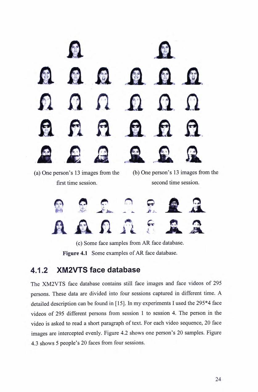
4.1.2 XM2VTS face database The XM2VTS face database contains still face images and face videos of 295

persons. These data are divided into four sessions captured in different time. A

detailed description can be found in [15]. In my experiments I used the 295*4 face

videos of 295 different persons from session 1 to session 4. The person in the

video is asked to read a short paragraph of text. For each video sequence, 20 face

images are intercepted evenly. Figure 4.2 shows one person's 20 samples. Figure

4.3 shows 5 people's 20 faces from four sessions.

24

MMMMM _ 圓 _ 國 _

• _ _ _ 國

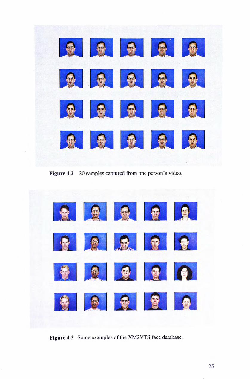
國 _ _ _ _ Figure 4.2 20 samples captured from one person's video.

_ _ _ _ _

l^wiW,””� PWBWiPi I^JjJJ^"^

翻 園 l i U 觀 i k i

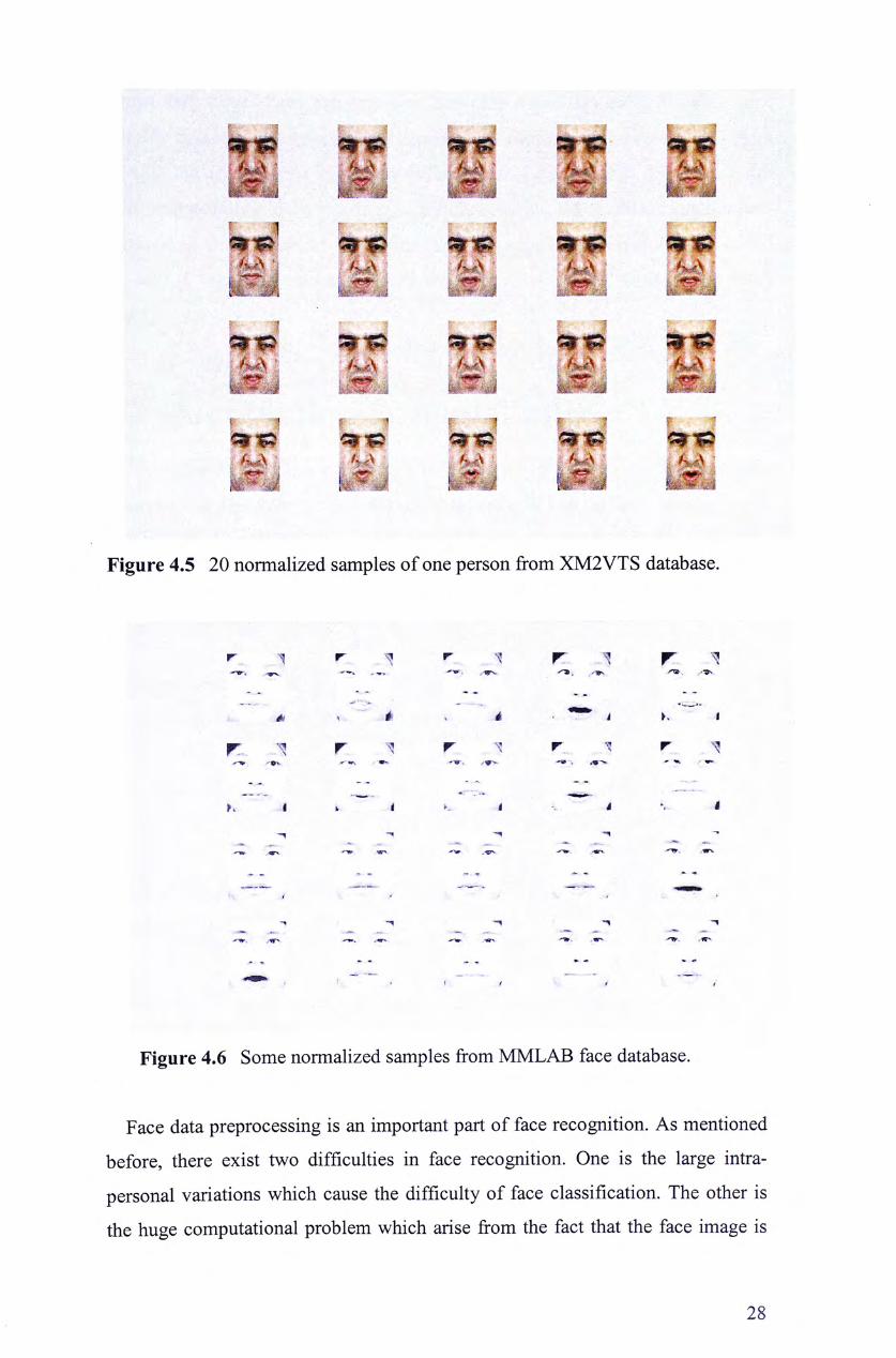
Figure 4.3 Some examples of the XM2VTS face database.

25

4.1.3 MMLAB face database

For face recognition research our lab has built a face-based video sequence

database, the MMLAB face database. It is divided into the first time session and

the second time session. The first time session is composed of 172*10 video

sequences of 172 different persons. The second time session is composed of

72*10 video sequences of 72 different persons who appeared in the first time

session. All video sequences are captured under the same configurations and

without any decoration on the face (i.e., glasses, scarf). There is at least a gap of

one month between the first time session videos and the second time session

videos. The duration of each video sequence is 20 seconds. The detailed

description is shown in Table 4.2.

Table 4.2 Description of the ten face videos.

Sequence ID Description 1 Neutral expression 2 Free expression (change expressions

randomly). 3 Reading a paragraph of text with

neutral expression. 4 Reading a paragraph of text with happy

expression. 5 Reading a paragraph of text with sad

expression. 6 Reading a paragraph of text with angry

expression. 7 Reading a paragraph of text with

surprised expression. 8 Neutral expression following a moving

target. 9 Reading a paragraph of text with

neutral expression while following a moving target.

Repeat Neutral expression

For each video sequence, 50 face images are intercepted evenly during the 20

seconds period.

26

；,J �y ； ••• / 心 / •‘多 “T f J： ”秦

t s f y ，.：/ ^ y ’：f � ‘/

p m M

p ^ p

. /！ ‘灰 4 A \ _ , A _ k h _

Figure 4.4 Some examples of MMLAB face database.

4.1,4 Face Data Preprocessing The procedure of face data preprocessing can be described as the follows:

Scale the face image so that the distance between two eyes is a constant, 45

pixels.

Crop the face from the original face image according to the location of the

midpoint of the two eyes.

•：• Perform histogram equation on the cropped image to reduce the lighting

variations in some way.

After preprocessing, each face image is normalized and aligned by size. Figure

4.5 shows the normalized samples of the face images in Figure 4.2. Figure 4.6

shows the normalized samples of the face images in Figure 4.4.

27

U • b d M m ^ . y j

iMi k^i ^ 翻 麥 肩 r ？ I r' I f 1 ^^ ‘ snrii ini i/玄i � c M i k^J fe^i y^J ‘色； fc^ f 1 ^ r I F ‘ 1

_ 舊 • ， sr穆 mm 勞養 t ‘ /v 為'‘ hJs * t '： ^^ I h^'J • ffTj •梦』 ^ m j 5 1 I 1 r 1 r I I 1

序 IP ？ 、丨 广 . J ‘ � �J • ^ �： . fikA ‘ k ^ j 胸 mJ 圓 LU

Figure 4.5 20 normalized samples of one person from XM2VTS database.

r 1 r r 1 r r

m � • i • i K 1

r 1 r r r r i 嫌• •.勢 -— — •• -

K 1 I. i — i i V I

1 ， -， ， ，

- - ，等 -» -

“ 棚 / » /

Figure 4.6 Some normalized samples from MMLAB face database.

Face data preprocessing is an important part of face recognition. As mentioned

before, there exist two difficulties in face recognition. One is the large intra-

personal variations which cause the difficulty of face classification. The other is

the huge computational problem which arise from the fact that the face image is

28

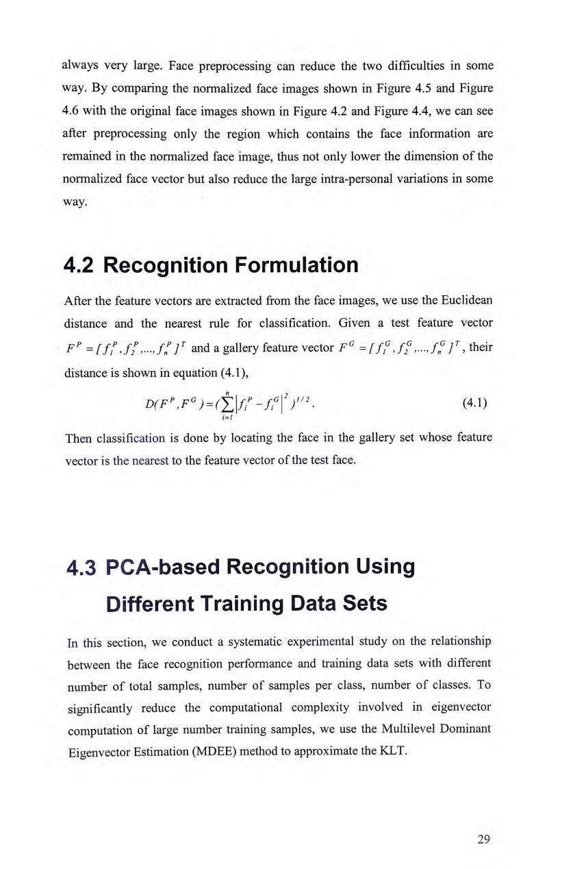
always very large. Face preprocessing can reduce the two difficulties in some

way. By comparing the normalized face images shown in Figure 4.5 and Figure

4.6 with the original face images shown in Figure 4.2 and Figure 4.4，we can see

after preprocessing only the region which contains the face information are

remained in the normalized face image, thus not only lower the dimension of the

normalized face vector but also reduce the large intra-personal variations in some

way.

4.2 Recognition Formulation After the feature vectors are extracted from the face images, we use the Euclidean

distance and the nearest rule for classification. Given a test feature vector

:[f[\f�’…’ fn']' and a gallery feature vector F�=厂 /广//，..”/f 广，their

distance is shown in equation (4.1),

(4.1) i=l

Then classification is done by locating the face in the gallery set whose feature

vector is the nearest to the feature vector of the test face.

4.3 PCA-based Recognition Using Different Training Data Sets

In this section, we conduct a systematic experimental study on the relationship

between the face recognition performance and training data sets with different

number of total samples, number of samples per class, number of classes. To

significantly reduce the computational complexity involved in eigenvector

computation of large number training samples, we use the Multilevel Dominant

Eigenvector Estimation (MDEE) method to approximate the KLT.

29

4.3.1 Experiments on MMLAB Face Database

4.3.1.1 Training Data Sets and Testing Data Sets

For the experiments, we use images of 100 people in the first session as training

data, and use images of the other 72 people as testing data. There is no overlap

between the two data sets.

In order to evaluate the influence of different training data sets on the

recognition accuracy, we select different subsets from the training data set for the

experiments. We design two training data sets with each containing 3 subsets, as

shown in Table 4.3. For the first training data set, we fix the number of total

training samples and then change the class number and samples per class in each

training subset. For the second training set, we fix the number of classes and

change the number of samples per class in each training subset.

For testing data, we use the same testing data set for all experiments. The

testing data set is composed of a gallery set and a probe set. The gallery set

contains 72*10 face images of 72 different persons from the first session. The

probe set contains 72*10 images of the same 72 persons from the second session.

All the face images of the testing data set have not appeared in the training data

sets.

Table 4.3 Different training data sets from MMLAB face database.

“ ^ “ N u m b e r of all . . , ^ . Number of Training data sets , ,本 Number of classes i , samples per subset samples per class Subset 1000 100 10

Training ^ , data set = � � lOOO 50 20

#1 _ _ ^ Subset 1000 20 50

#3 Subset 100 100 1

T . . #4 Training . . data set 加么set lOOO 100 10

#2 控 SiiVKet iUDsei 5000 100 50

#6

30

4.3.1.2 Face Recognition Performance Using Different

Training Data Sets

The face recognition results based on training data set #1 is shown in Table 4.4

and Figure 4.7. For the three different training subsets, we compare their

recognition performance using a number of different eigenfeature numbers

ranging from 20 to 1000. A probe image is considered correctly recognized if it

matches any one of the ten images of the same person in the gallery set. The

absolute accuracy is not important in the experiments. We intentionally use

difficult data containing large facial expression changes to lower the overall

recognition accuracy in order to compare the relative performance of different

experiments.

From the results, we can see that the training subset #1 is slightly better than

#2, which in turn is slightly better than #3, especially when the feature length is

small. This shows that using images from more people can better characterize the

eigenspace because of more inter-person variations in the training data set.

The face recognition results based on training data set #2 is shown in Table 4.5.

The results seem again confirm what we observe in Table 4.4. If we look at the

results below feature length 100, the three tests are fairly compatible. This shows

that simply increasing the number of images per person will not affect the

recognition results much. The number of people seems more important.

We focus more on the results of short feature lengths since they illustrate how

efficient the transformation compress the large face vector. As the length of the

feature vector increases, it becomes more like the original face vector. The effect

of the transformation is largely lost. In fact, if we use the original face image

directly for face recognition, we get an accuracy of 74.9%, which is actually the

upper limit of the eigenface results. The advantage of the eigenface approach is

not at improving the recognition accuracy, but rather is at improving the

computational efficiency. We can use a feature vector of a few hundreds values to

achieve comparable performance of the original image with thousands of pixels.

31

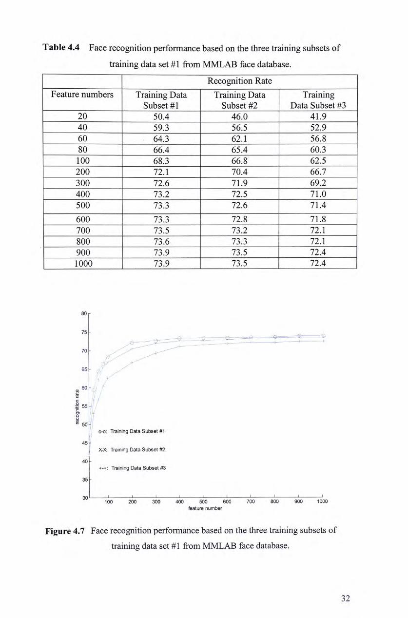
Table 4.4 Face recognition performance based on the three training subsets of

training data set #1 from MMLAB face database.

Recognition Rate Feature numbers Training Data Training Data Training

Subset #1 Subset #2 Data Subset #3 — 20 50.4 “ 46.0 41.9 “ — 40 59.3 56.5 52.9

60 64.3 “ 62.1 56.8 “ — 80 66.4 65.4 60.3 “

100 68.3 66.8 62.5 一

200 72.1 “ 70.4 66.7 一

300 72.6 71.9 69.2 — — 400 73.2 72.5 一 71.0

^ 7L4 一 600 73.3 72.8 71.8 ~ 700 73.5 “ 73.2 72.1 “

800 73.6 73.3 72.1 “ 900 73.9 — 73.5 ~ 72.4

— 1000 73.9 73.5 72.4 “

80「

75 - ^ „ « P,_

7:^1：：：===^^^』::::^=^—^^^^ 7 � - / ^ Z 65 _ 6丫 Z

!J , /

2 u / | 5 “ " 1

I //f Ij 0-0： Training Data Subset #1

45 -X-X Training Data Subset #2

40 -+-+: Training Data Subset #3

35 -

30 I I I I I I I 1 1 1 100 200 300 400 500 600 700 800 900 1000

feature number

Figure 4.7 Face recognition performance based on the three training subsets of

training data set #1 from MMLAB face database.

32

Table 4.5 Face recognition performance based on the three training subsets in

training data set #2 from MMLAB face database.

Recognition Rate (%) Feature numbers Training Data Training Data Training

Subset #4 Subset #5 Data Subset #6 — 20 — 51.7 ~ 50.4 49.7

40 一 57.7 59.3 一 59.6 — 60 一 61.1 — 64.3 一 64.7 — 80 64.3 66.4 66.8 “ — 100 68.1 68.3 68.2 “

^ MUi m

^ N d i ^ m 400 N d i m ^ N ^ ^ 700 N ^ ^ ^ ^ 1000 ^ 2000 ^

Null Null 4000 Null ^ 5000 ^

4.3.2 Experiments on XM2VTS Face Database We also perform the experiments on the XM2VTS face database. Similar to

MMLAB face database, we design two training data sets with each containing 4

subsets, as shown in Table 4.6. For the first training data set, we fix the number of

total training samples and then change the class number and samples per class in

each training subset. For the second training set, we fix the number of classes and

change the number of samples per class in each training subset.

For testing data, we use the same testing data set for all experiments. The

testing data set is composed of a gallery set and a probe set. The gallery set

contains 95 face images of 95 different persons from the first session. The probe

set contains 95*20 images of the same 95 persons from the second session. All the

face images of the testing data set have not appeared in the training data sets.

33

The face recognition result based on training data set #1 is shown in Table 4.7

and Figure 4.8 and the result based on training data set #2 is shown in Table 4.8.

Here we want to emphasize again that the absolute accuracy is not important for

this experiments. We intentionally use difficult data to lower the overall

recognition accuracy in order to compare the relative performance of different

training data. Experimental results on XM2VTS face database seem again confirm

what we observe in the experiments on MMLAB database.

Table 4.6 Different training data sets from XM2VTS face database.

T . • 7~ ‘ N u m b e r of all H I ‘ 7", Number of Training data sets , , 丄 Number of classes , . : samples per subset samples per class Subset 400 ^ 2

Training ^ data set Subset 400 50 8

#1 Subset 400 20 20

m Subset 400 ^ 2

Training ^ data set Subset 1000 200 5

#2 Subset 4000 200 20 #6

Table 4.7 Face recognition performance based on the three training subsets of

training data set #1 from XM2VTS database.

Recognition Rate (%) Feature numbers Training Data Training Data Training Data

Subset #1 Subset #2 Subset #3 — 20 50.1 “ 48.4 47.1 “ — 40 56.2 “ 52.6 48.5 “ — 60 57.6 “ 53.8 49.0 — 80 58.8 - 54.9 一 51.0 一

— 100 59,8 — 55.8 一 52.1 一

— 120 60.2 “ 56.8 52.2 140 60.6 “ 57.0 52.5

— 160 60.4 — 57.1 53.2 — “ 180 60.4 57.9 53.6 一

~ 200 60.1 “ 58.1 54.2 — 250 60.3 - 58.3 54.4 一

^ ^ ^ 一 350 60.4 — 58.3 55.6 一

— 399 60.6 58.3 55.5 一

34

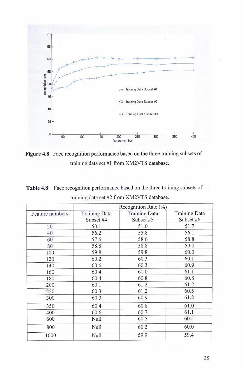
70 r

65 -

60 - ^ ― ~ ^ ― ^ ^ & ^ 一 )

声 , ^ . “ “ — — — 一 ― — — 一 — — 一 —

5 5 - z ^ z _ _ _ — — 一 一 — — — — H 卜

二 I, _斗一 ^ ^ [ / /

:| 崎 / / 0 ‘ ^ 0-0； Training Data Subset #1 £ “

45 -X-X: Training Data Subset #2

40 -

-K+: Training Data Subset #3

35 -

3 0 I I I I I 1 1 1 50 100 150 200 250 300 350 400

feature number

Figure 4.8 Face recognition performance based on the three training subsets of

training data set #1 from XM2VTS database.

Table 4.8 Face recognition performance based on the three training subsets of

training data set #2 from XM2VTS database.

Recognition Rate (%) Feature numbers Training Data Training Data Training Data

Subset #4 Subset #5 Subset #6 — 20 50.1 - 51.0 一 51.7 — 一 40 56.2 “ 55.8 56.1 “ — 60 57.6 58.0 — 58.8 一

— 80 58.8 - 58.8 59.0 “ — 100 59.8 - 59.8 — 60.0 — — 120 60.2 60.3 60.1 “ — 140 60.6 - 60.3 60.9 — 160 60.4 - 61.0 61.1 “ 180 60.4 - 60.8 一 60.8 — — 200 60.1 _ 61.2 — 61.2 一

_ 250 60.3 “ 61.2 — 60.5 — ^ 612

“ 350 60.4 — 60.8 “ 61.0 — 400 60.6 60.7 — 6L1 —

^ ^ ^ ^ Mdi ^ ^

Null ^ ^

35

4.3,3 Comparison of MDEE and KLT In this section we use a simple experiment to illustrate that the MDEE method is a

very close approximation of the KLT method. We apply MEDD and KLT

separately on the same training data set selected from MMLAB face database:

1000 face images from 100 different people with 10 face images per person.

Figure 4.9 shows that the values of the top 300 eigenvalues computed by the

MDEE and KLT. The results of the two methods are nearly identical. The

recognition results are shown in Table 4.9. Again, the results are nearly the same.

From Figure 4.9 and Table 4.9, we can see that the performance of MDEE and

KLT are very similar and MDEE is indeed a very close approximation of KLT.

Table 4.9 Recognition rate comparison of MDEE and KLT.

Recognition Rate (%) — F e a t u r e Numbers MDEE KLT 一

— 20 “ 50.1 50.1 “ — 40 59.3 59.3 “ — 60 64.3 64.3 一

— 80 66.4 — 66.4 一

— 100 68.5 68.3 一

200 111 72.1 300 ‘ 73.0 72.6 一

400 73.2 — 73.2 一

500 “ 73.3 73.3 一

600 73.6 73.3 — 700 “ 73.9 73.5 一

— 800 73.9 73.6 一

— 900 74.2 73.9 一

“ 1000 74.2 73.9

36

22� 22�

I , I , — — 吾 1 6 - - 1 6 -

呈 I 14 - 0 - 0 : MDEE 14 - 0 - 0 : MDEE

X-X: KLT X-X: KLT

12- 12 -

10 I ‘ ‘ ‘ ‘ ‘ ‘ ‘ ‘ ‘ ‘ 10 I I 1 i 1 « 1 1 “ 1 ‘ 0 5 10 15 20 25 30 35 40 45 50 55 60 6 5 70 75 80 8 5 90 95 100

feature number feature number

(a) (b)

2 2 r 22 r

. 20 • 20 -

18 - 18 -

I I ^ .. 1., .,, . ............--……

W S' - ' - - - ‘…！ r!M.(,..:i.�.C:.

14 - 0 - 0 : MDEE 14 . 0 - 0 : MDEE

X-X: KLT X-X: KLT

12 - 12 -

105 110 115 120 125 130 135 140 145 150 155 i g o 165 170 175 1 80 185 190 195 200 feature number feature number

(C) (d)

22� 22�

20 - 20-

16 - 0 -0 : MDEE 18 - 0 -0 : MDEE

g X-X: KLT I X-X: KLT

£ 16- |16-I ..…-.……… I

12. 12-

10 205 210 215 220 225 230 235 240 245 250 255 260 265 270 275 280 285 290 295 300 feature number feature number

(e) (f)

Figure 4.9 (a)-(f): Top 300 eigenvalues of MDEE and KLT.

37

4.3,4 Summary

In this section, we explored the relationship between the PCA-based recognition

performance and different training data sets. Using the MDEE algorithm we are

able to compute eigenfaces from a large number of training samples. This allows

us to compare the recognition performance using different training data sizes.

Experimental results based on the MMLAB face database and the XM2VTS face

database show that simply increasing the number of face images per person will

not affect the recognition results much. The number of different people used in the

training data is more important since using images from more people can better

characterize the eigenspace because of more inter-person variations in the training

data set.

4.4 LDA-based Recognition Using Different Training Data Sets

4.4.1 Experiments on AR Face Database In this section we will use the AR face database to investigate the relationship

between the LDA-based recognition and different training data sets.

4A1.1 Selection of Training Data and Testing Data

For the AR face database, there are totally 90 persons who have complete face

sequences from both sessions. Here we select the training data and the testing data

from the face images of these 90 persons.

For the training data, we design three different training data sets. For the

training data sets #1，we select 90*4 face images of 90 persons from the first

session. These images only contain expression variations. For the training data

sets #2, we select 90*4 face images of 90 persons from the first session, but these

images contain the lighting variations. For the training data sets #3，we select

90*7 face images of 90 persons. These images contain not only the expression

variation but also the lighting variations. The detailed description of the training

data is shown in Table 4.10.

38

For the testing data, which is composed of a gallery set and a probe set. The

gallery set is composed of 90 normal face images of 90 persons from the first

session. The probe set is composed of 90*7 face images of 90 persons form the

second session. The face images of the probe set contain not only the lighting but

also the expression variations. The detailed description of the training data is

shown in Table 4.11.

Table 4.10 Training data structure.

Training Session Face ID Description Size Data Set

¥l 1 1,2,3,4 Only expression variation

—#2 — 1 1,5,6,7 Lighting variation “ 90*4 “ m 1 1,2,3,4,5,6,7 Expression and

lighting variation

Table 4.11 Testing data structure.

Testing Session ID Description Size data

Gallery set 1 1 Neural Expression 90 Probe set 2 14,15,16,17,18,19,20 Expression and W l

lighting variation

4.4.1.2 LDA-based recognition on AR face database

Experimental results based on the three different training data sets of AR face

database are shown in Table 4.12. We use the number of principal components

from 90 to 540 in the PCA step, then select 89 (class number minus 1) features in

the following FLD analysis to compare the relative accuracy of the three different

training data sets. From the results, we can see that the recognition performance of

the training data set #2 is better than the training data set #1，and the recognition

performance of the training data set #3 is much better than the training data set #1

and the training data set #2. The reason for this behavior is that the training data

set #2 capture the lighting variations which are much larger than the expression

variations captured by the training data set #1, and the training data set #3

captured the largest variation among the three training data sets. This shows that

39

increasing the variety of the training data will benefit the LDA-based recognition.

The variety of the training data plays a key role in LDA-based recognition.

Table 4.12 Recognition accuracy of different training data from Purdue database.

PCA dimension Training Data Training Data Training Data

for FLD analysis Set#l Set #2 Set #3

% 50.2% 65.7% 70.3%

50.0% 67.8% 74.0%

56.0% 68.9% 74.8%

56.0% 68.9% 76.0%

^ 56.4% 68.1% 77.0%

^ 54.0% 67.3% 76.8%

^ 54.3% 68.1% 78.9%

^ N ^ 78.9%

^ T ^ 79.8%

^ MUi 81.1%

4.4.2 Experiments on XM2VTS Face Database In last section, we have evaluated the LDA method based on AR face database

and draw the conclusion that increasing the variety of the training data will benefit

the recognition performance. However, our conclusion is still limited by the size

of the AR face database. To further explore the relationship between the LDA

method and different training data we need a much larger database. Here we will

evaluate the LDA method based on the video sequences of XM2VTS database

[15]. Since we need a large number of samples for each person, the video data in

the XM2VTS database is perfect for our experiments. We select 295*4 video

sequences of 295 different persons from the four sessions captured in different

time. Each person in the video is asked to read a short paragraph of text. For each

video sequence, 20 face images are intercept evenly and then normalized by size.

40

4.4.3 Training Data Sets and Testing Data Sets Similar to the FERET test we divide the XM2VTS database into development

portions and sequestered portions. The development portion is used for training

and the sequestered portion is used for generality test. The division scheme is

shown in Table 4.13.

Table 4.13 The division scheme of development and sequestered portions.

Data subset Number of people Total number of images

Development portion ^ 200*20

Sequestered portion 95 95*20

In order to evaluate the influence of different training data sets on the

recognition accuracy, we design three sets of training data. For the first set, we

select all data from the first session and choose different number of samples per

person as 3，5，10, and 20. For the second set, we select the data from both the

first session and the fourth session. For the third set, we select the data from both

the first session and the third session. Table 4.14，Table 4.15, and Table 4.16 show

the structures of the three training data sets.

The testing data is composed of a probe set and a gallery set. The gallery set is

composed of 95*20 images of the development portion's 95 people from the first

session and the probe set is composed of 95*20 images of the same 95 people

from the fourth session.

Table 4.14 Training data set #1.

Training Data Session Number of Number of Total samples

Set samples per classes

# 1 class

Subset #1 F ^ 3 ^ ^

Subset #2 FkS 5 ^

Subset #3 Fii^ 10 ^ 2000

””Subset #4 F i ^ ^ ^

41

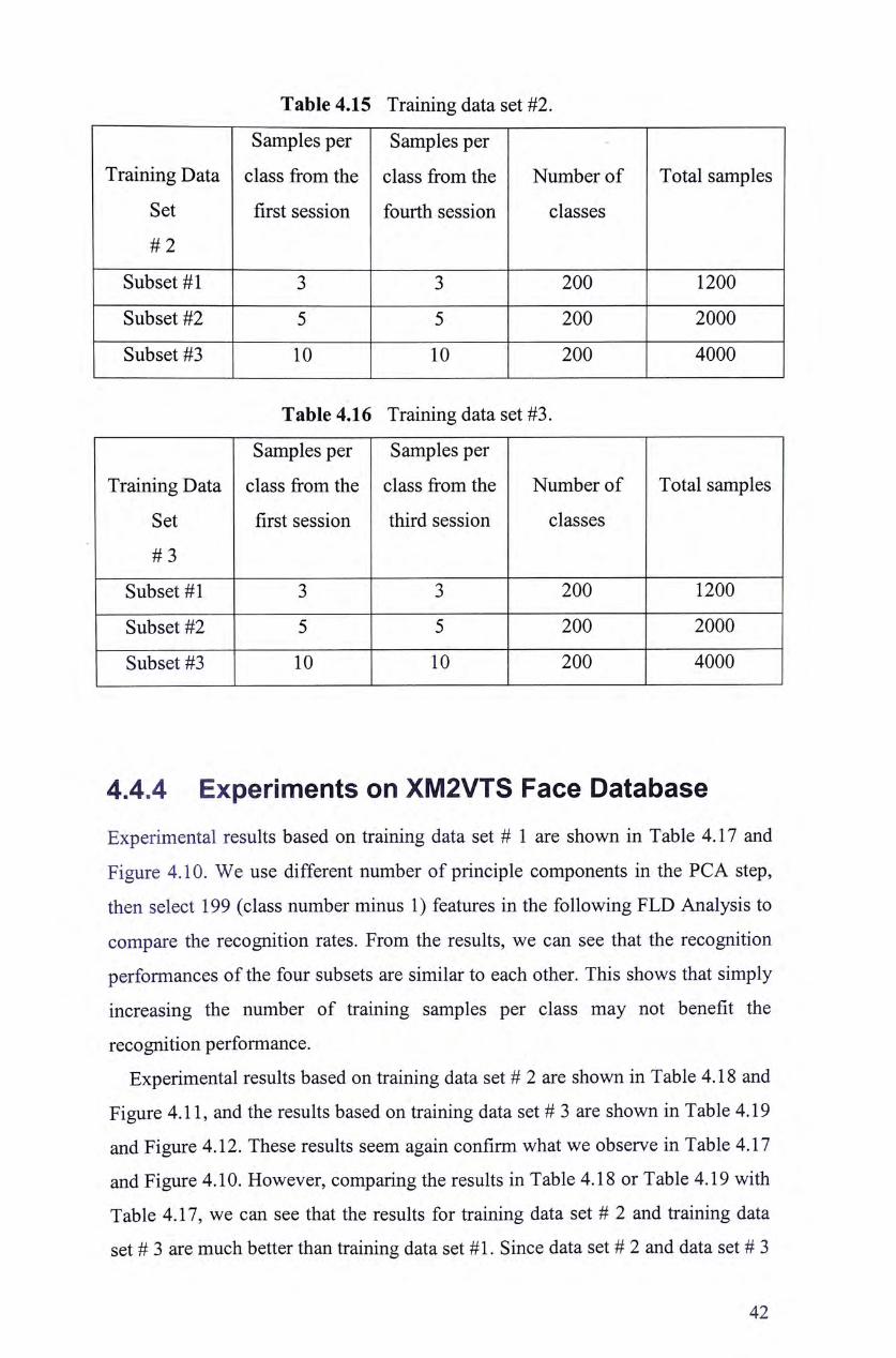
Table 4.15 Training data set #2.

Samples per Samples per

Training Data class from the class from the Number of Total samples

Set first session fourth session classes

#2

Subset #1 3 3 ^

Subset #2 r 5 ^ 2000

Subset #3 10 10 ^ 4000

Table 4.16 Training data set #3.

Samples per Samples per

Training Data class from the class from the Number of Total samples

Set first session third session classes

# 3

Subset #1 3 3 ^

Subset #2 5 5 ^

Subset #3 10 10 ^ 4 0 ^

4.4.4 Experiments on XM2VTS Face Database Experimental results based on training data set # 1 are shown in Table 4.17 and

Figure 4.10. We use different number of principle components in the PCA step,

then select 199 (class number minus 1) features in the following FLD Analysis to

compare the recognition rates. From the results, we can see that the recognition

performances of the four subsets are similar to each other. This shows that simply

increasing the number of training samples per class may not benefit the

recognition performance.

Experimental results based on training data set # 2 are shown in Table 4.18 and

Figure 4.11, and the results based on training data set # 3 are shown in Table 4.19

and Figure 4.12. These results seem again confirm what we observe in Table 4.17

and Figure 4.10. However, comparing the results in Table 4.18 or Table 4.19 with

Table 4.17, we can see that the results for training data set # 2 and training data

set # 3 are much better than training data set #1. Since data set # 2 and data set # 3

42

contain data from different sessions, they can capture the intra-personal variation

across different sessions precisely, thus are able to help to reduce such variation in

the within class matrix whitening step of LDA. Simply increasing sample

numbers in the same session cannot help to capture such cross session variation.

The intra-personal variation caused by expression change in the same video can

seem to be represented by a small number of samples per person.

Table 4.17 Recognition performance of training data set #1.

P ^ Subset # 1 S u b s e t # 2 S u b s e t # 3 S u b s e t #4 dimension for FLD analysis

^ 87.5% 85.9% 85.3% 85.0%

^ 88.8% 85.1% 84.1% 83.7%

^ 88.1% 84.1% 83.1% 83.4%

88.0% 84.3% 83.1% 83.7%

85.9% 84.0% 82.4% 83.6%

^ ^ ‘ 83.2% 81.2% 81.0%

^ N ^ 80.0% 80.7% 79.2%

79.4% 78.5%

^ ^ 78.0% 78.6%

1 I 1 1 1 1 1 1 1 1 1

0.95 - -

0.9 - 丄 -“------+-

0.75 - -

Hh： T ra in ing Data S u b s e t #1 ^ 0.7 - -

^ Tra in ing Data S u b s e t 沿

0.65 - -

0-0： Tra in ing Data S u b s e t 沼

0 . 6 - -

x-x: Tra in ing Data S u b s e t #4 0.55 - -

n 5 1 1 1 1 1 1 1 ' ‘ '200 3 0 0 4 0 0 5 0 0 6 0 0 7 0 0 8 0 0 9 0 0 1 0 0 0 1 1 0 0 1 2 0 0

The numbe r of s e l e c t e d P C s

Figure 4.10 Recognition performance of training data set #1.

43

Table 4.18 Recognition performance of training data set #2,

PCA dimension Subset #1 Subset #2 Subset #3 for FLD analysis

^ 94.0% 93.4% 93.7%

^ 95.3% 94.8% 95.0%

^ 94.7% 95.0% 95.3%

94.6% 94.8% 95.3%

400 94.3% 95.8% 95.8%

600 Mdi 95.5% 95.7%

94.1% 94.4%

Null N ^ 94.6%

N ^ 93.1%

N^ Null Null

r ^ ^ N^

1 —•—I 1 1 1 1 1 1 1 1

0.95 一 ： 卜 -'• ______ 义 J

0.9 - -a> 2 +-+: Training Data Subset #1 [

0.85 - -

S Training Data Subset #2 cS

0 . 8 - -

0-0： Training Data Subset #3

0.75 - -

• 7 I 1 1 1 I I 1 1 1 •2 0 0 300 400 500 600 700 800 900 1000 1100 1200

The number of selected PCs

Figure 4.11 Recognition performance of training data set #2.

44

Table 4.19 Recognition performance of training data set #3.

PCA d i m e n s i o n S u b s e t #1 Subset #2 Subset #3 for FLD analysis

^ 92.7% 93.9% 93.9%

^ 93.6% 94.2% 94.3%

^ 93.5% 94.5% 94.5%

94.0% 94.2% 94.5%

94.3% 94.6% 96.2%

^ 92.4% 94.2%

MUi 90.8% 93.0%

1000 N ^ Null 93.2%

" m i ^ 91.8%

1 1 1 1 1 1 1 1 1 1 ‘

声------

.”一f"tj：：*-办--、、 、务-----一一〜

0.9 - -

•K+: Training Data Subset #1

c I 0.85 - -

O

羞 *-*: Training Data Subset #2

0 , 8 - -

0-0： Training Data Subset #3

0.75 - -

0 7 I I I i I I I 1 1 '200 300 400 500 600 700 800 900 1000 1100 1200

The number of selected PCs

Figure 4.12 Recognition performance of training data set #3.

45

4.4.5 Summary In this chapter we investigated the relationship between LDA-based face

recognition method and different training data sets. We use two famous face

databases: AR face database and XM2VTS face database to evaluate the LDA

method. Using the AR face database, we can design different training data sets

with different intra-personal variations. Experimental results on the AR face

database show that increasing the variety of training data will benefit the LDA

recognition performance. Using the XM2VTS database, we can obtain a set of

long face sequences. This allows us to compare LDA-based recognition

performance using different training data sizes. Experimental results on the

XM2VTS face database show that simply increasing the number of samples per

class from the same session will not benefit the recognition performance. The

important factor is not the number of images, rather is the variety of the training

data. By selecting the training data from different sessions, we can capture the

intra-personal variation that exists between the testing and gallery data, thus give

much better recognition performance.

46

Chapter 5

Summary Similar to other pattern recognition problem, face recognition depends heavily on

the selection of face feature vectors, e.g. PCA-based vectors and LDA-based

vectors. Since these feature vectors are computed directly from the training face

images, it is reasonable to expect that the recognition performance may be

influenced by different training data sets. However, until now most previous

researches simply choose a small number of training samples randomly for

computation of the feature vectors without much justification.

In this thesis, we explore this meaningful and important topic. We conduct a

systematic experimental study on the relationship between face recognition

performance and different training data sets. During the past thirty years

researchers have proposed a number of face recognition techniques among which

PCA-based and LDA-based techniques are among the most popular and

successful ones. Especially in recent years many proposed novel face recognition

techniques are related to the PCA technique or the LDA technique. Therefore in

this thesis we select these two representative techniques for the comparison of the

recognition performance of different training data sets.

For the both techniques: PCA and LDA, it is generally believed that the size of

the training data play a key role for the recognition performance. Here we show

that it is not always the case. Experimental results show simply increasing the

number of training samples per person does not help to improve the recognition

performance.

For the PCA-based technique, to overcome the computational problem we use

the MDEE algorithm to compute the eigenfaces from a large number of training

samples. This allows us to compare the recognition performance using different

training data sizes. Experimental results show that using images from more people

can better characterize the eigenspace because of more inter-personal variations

contained in the training data. Simply increasing the number of face images per

person will not affect the recognition results much. Generally increasing the

47

number of people benefits the recognition performance more than increasing the

number of images per person.

For the LDA-based technique, experimental results show that simply increasing

the number of samples per class from the same session will not benefit the

recognition performance. The important factor is not the number of images,

rather is the variety of the training data. By selecting the training data from

different sessions, we can capture the intra-personal variation that exists between

the testing and gallery data, thus give much better recognition performance.

My work will benefit the improvement of face recognition performance and

efficacy by choosing appropriate training data. Especially it may benefit the

research on face recognition in video where large amount of face images are

involved.

48

Bibliography :1] R. Chellappa, C. L. Wilson, and S. Sirohey, "Human and machine

recognition of faces: a survey," Proceedings of the IEEE, Vol. 83, pp. 705-

741，May 1995.

'2] W. Zhao, R. Chellappa, and P. Philips, “Face recognition: a literature

survey；' UMD CfAR Technical Report CAR-TR-948, 2000

3] R. Baron, "Mechanisms of human facial recognition," Int. J. Man Machine

Studies, Vol. 15. 137-178，1981.

4] M. Turk and A. Pentland, "eigenfaces for recognition," J. of Cognitive

Neuroscience, vol. 3, no. 1，1991.

:5] M. Turk and A. Pentland "Face Recognition Using Eigenfaces," in Proc. of

IEEE International Conference Computer Vision and Pattern Recognition,

pp. 586-591,1991.

[6] A. Pentland, B. Moghaddam, and T. Stamer, "View-Based and Modular

Eigenspaces for Face Recognition," Proc. IEEE Conf. CVPR, 1994.

[7] R. Bmnelli and T. Poggio, "Face Recognition: Features vs. Templates,"

IEEE Trans, on PAMI, vol. 15，no. 10, Oct. 1993.

8] Martinez and R. Benavente, “The AR Face Database," CVC Technical

Report #24, Purdue University, June 1998.

[9] D. L. Swets and J. Weng, “Using discriminant eigenfeatures for image

retrieval," IEEE Transactions on Pattern Analysis and Machine Intelligence,

Vol. 18, pp. 831-836, Aug. 1996.

10] P. Belhumeur, J. Hespanha, and D. Kriegman. "Eigenface vs. Fisherfaces:

Recognition Using Class Specific Linear Projection", IEEE Trans. Pattern

Analysis and Machine Intelligence, 19(7): 711-720，1997.

[11] K. Etemad and R. Chellappa. "Discriminant analysis for recognition of

human face images，，，Journal of the Optical Society of America A, 14(8):

1724-1733，1997.

[12] W. Zhao, and R. Chellappa. “Discriminant Analysis of Principal

Components for Face Recognition," IEEE Conf. Automatic Face and

Gesture Recognition, Page(s): 336 -341, 1998.

49

13] R. Fisher, "The use of multiple measures in taxonomic problems," Ann.

Eugenics, vol. 7, pp.179-188, 1936.

14] M. Kirby, and L. Sirovich, "Application of the Karhunen-Loeve procedure

for the characterization of human faces," IEEE Trans, on Pattern Analysis

and Machine Intelligence, vol. 12, no. 1, pp. 103-108, Jan. 1990.

[15] K. Messer, J. Matas，J. Kittler, J. Luettin, and G. Matitre. “XM2VTSDB:

The Extended M2VTS Database," Second International Conference on

Audio and Video-based Biometric Person Authentication, March 1999.

16] L. Wiskott, "Phantom faces for face analysis," Proc. of International

Conference on Image Processing, Vol. 3, pp. 308-311, 1997.

17] X. Tang, "Texture information in run-length matrices," IEEE Transactions

on Image Processing, vol. 7，No. 11, pp. 1602-1609, Nov. 1998.

18] K. Fukunnaga, Introduction to Statistical Pattern Recognition, Academic

Press, second edition, 1991.

19] M. Lades, J. C. Vorbruggen, J. Buhmann, J. Lange, C. D. Malsburg, R. P.

Wurtz, W. Konen, "Distortion invariant object recognition in the dynamic

link architecture," IEEE Trans, on Computers, Vol. 42, pp. 300-311, Mar.

1993.

'20] L. Wiskott, J. M. Fellous, N. Kniger, and C. von der Malsburg, "Face

recognition by elastic bunch graph matching," IEEE Trans, on PAMI, Vol.

19, No. 7, pp. 775-779，1997.

21] J. Zhang, Y. Yan, and M. Lades, "Face recognition: eigenface, elastic

matching, and neural nets，，’ Proceedings of the IEEE, Vol. 85, pp. 1423-

1435，Sept. 1997.

22] B. Moghaddam, and A. Pentland, "Probabilistic visual learning for object

representation," IEEE Trans, on PAMI, Vol. 19, No. 7, pp. 696-710, July

1997.

；23] B. Moghaddam, W. Wahid, and A. Pentland, “Beyond eigenfaces:

probabilistic matching for face recognition," IEEE Conf. Automatic Face

and Gesture Recognition, pp. 30-35, 1998.

[24] C. Liu and H. Wechsler, “Enhanced Fisher Linear Discriminant Models for

Face Recogniiton," Proc. ICPR, Vol. 2，pp. 1368-1372, 1998.

50

25] C. Liu and H. Wechsler, "Evolutionary pursuit and its application to facer

recognition," IEEE Trans, on PAMI, Vol 22，No. 6, pp. 570-582, 2000.

[26] A. Martinez, and A. Kark, “PCA versus LDA," IEEE Trans, on PAMI, Vol.

23, No. 2，pp. 228-233,2001.

：27] J. Yang, H. Yu, and W. Kunz, "An Efficient LDA Algorithm for Face

Recognition," Proc. of International Conference on Pattern Recognition,

2002.

28] Yu Bing, Jin Lianfu, and Chen Ping, “A New LDA-based Method for Face

Recognition," Proc. of International Conference on Pattern Recognition,

2002.

；29] H. Kim, D. Kim, S. Y. Bang, "Face Recognition Using LDA Mixture

Model," Proc. of International Conference on Pattern Recognition, 2002.

[30] R‘ Huang, Q. Liu, H. Lu, S. Ma, “Solving the Small Sample Size Problem

of LDA," Proc. of International Conference on Pattern Recognition, 2002.

31] B. Moghaddam, "Principle manifolds and probabilistic subspace for visual

recognition," IEEE Trans, on Pattern Analysis and Machine Intelligence,

Vol. 24, No. 6, June, 2002.

[32] M. Yang, N. Ahuja, and D. Kriegman, "Face recognition using kernel

eigenfaces，，，Proc. oflCIP, Vol. 2, pp. 97-100, 2002.

'33] Q. Liu, R. Huang, H. Lu, and S. Ma "Face recognition using Kernel-based

Fisher Discriminant Analysis," Proc. of IEEE International Conference on

Automatic Face and Gesture Recognition，pp. 197-201, 2002.

'34] C. Liu, and H. Wechsler, "Robust coding schemes for indexing and retrieval

from large face databases," IEEE Trans, on Image Processing, Vol. 9, No. 1，

January, 2000.

'35] K. Etemad, and R. Chellappa, "Face recognition using discriminant

eigenvectors," Proc. ICASSP, Vol. 4, pp. 2148-2151, 1996.

36] K. Chung, S. Kee, and S. Kim, "Face recognition using principal component

analysis of Gabor filter responses," Proc. of International Workshop on

Recognition, Analysis, and Tracking of Faces and Gestures in Real-Time

Systems, pp. 53-57, 1999.

[37] M. Loeve, Probability Theory, Van Nostrand, Princeton, 1955.

38] I. T. Jolliffe, Principal Component Analysis, Springer-Verlag, New York,

1986. (Reference for PCA)

51

39] C. Liu, and W. H, “Gabor feature based classification using the enhanced

fisher linear discriminant model for face recognition," IEEE Trans, on

Image Processing, Vol. 11, Issue 4, pp. 467-476，April, 2002.

40] W. Lee, H. Lee, and J. Chung, "Wavelet-based FLD for face recognition,"

Proc. of IEEE Midwest Symposium on Circuits and Systems, Vol. 2, pp.

734-737, 2000.

41] W. Zhao, and R. Chellappa, "Robust image based face recognition," Proc.

oflCIP, Vol. 1，pp. 41-44, 2000.

42] M. J. Lyons, J. Budynek, A. Plante, and S. Akamatsu, "Classifying facial

attributes using a 2-D Gabor wavelet representation and discriminant

analysis," Proc. International Conference on Automatic Face and Gesture

Recognition, pp. 202-207, 2000.

43] W. Zhao, "Discriminant component analysis for face recognition," Proc. of

ICPR, Vol. 2，pp. 818-821，2000.

44] W. Zhao, and R. Chellappa, “Empirical performance analysis of linear

discriminant classifiers," Proc. ofCVPR, pp. 164-169，1998.

45] Zhao, W.; Nandhakumar, N. “Linear discriminant analysis of MPF for face

recognition," Proc. ICPR, Vol. 1, pp. 185-188, 1998.

[46] Zhifeng Li, and Xiaoou Tang, "Eigenface Recognition Using Different

Training Data Sizes," Proc. of the 2nd International Conf. on Information

Security, pp. 31-35, July 2002.

[47] Kun Ma, and Xiaoou Tang, “Discrete wavelet face graph matching," Proc.

oflCIP, Vol. 2, pp. 217-220, 2001.

'48] Zhifeng Li, and Xiaoou Tang, "LDA-based Face Recognition Using

Different Training Data Sets," Submitted to IEEE International Conference

on Acoustics, Speech, and Signal Processing, 2003.

[49] P. Phillips, H. Moon, P. Rauss, and S. Rizvi, “The FERET evaluation

methodology for face-recognition algorithms," Proc. of IEEE CVPR, pp.

137-143, 1997.

[50] P. Phillips, H. Moon, S. Rizvi, and P. Rauss, "The FERET Testing

Protocol," in Face Recognition: From Theory to Applications, H. Wechsler,

P. Phillips etc, pp. 244-261, Springer-Verlag, 1998.

52

'51] L. Okada, J. Steffens, T. Maurer, H. Hong, E. Elagin, H. Neven, and C. von

der Malsburg, “The Bochum/USC Face Recognition System And How it

Fared in the FERET Phase III test," in Face Recognition: From Theory to

Applications, H. Wechsler, P. Phillips etc, pp. 186-205, Springer-Verlag,

1998.

52] S. Lee, S. Jung, J. Kwon, and S. Hong, “Face Detection and Recognition

Using PCA,’，TENCON 99’ Proceeding of IEEE Region 10 Conference, Vol.

l ,pp. 84-87, 1999.

53

CUHK L i b r a r i e s

•DMDVbSTb