faceted semantic search - kitthe increasing amount of data on the web bears potential for addressing...
TRANSCRIPT

Technical Report
Faceted Semantic Search
by
Andreas Josef Wagner
Institute of Applied Informatics and Formal Description Methods
Faculty of Economics and Business Engineering
Karlsruhe Institute of Technology

Abstract
The increasing amount of data on the Web bears potential for addressing complex
information needs more effectively. Instead of keyword search and browsing along
links between results, users can specify their needs in terms of complex queries and
obtain precise answers right away. However, browsing is also essential on the Web
of data as users might not always know a specific query language and more im-
portantly, might not know the data. Particularly in cases where the information
need is fuzzy, browsing is useful for exploring the data. Faceted search allows users
to browse along facets. However, work on faceted search so far has been focused
on search rather than browsing. In this paper, we propose a facet ranking scheme
that targets the browsing experience. When there are too many facets given, user
obtain a ranked list of facets, where the rank represents the facets’ browse-ability.
Furthermore, facets might be associated with a large amount of values. Also target-
ing browse-ability, we propose clustering mechanisms to decompose such facets into
more fine-grained sub-facets. By means of a task-based evaluation, we demonstrate
that the proposed solution enables more effective browsing, when compared to the
state of the art that is rather focused on search-ability.

CONTENTS iii
Contents
List of Figures vi
List of Abbreviations vii
List of Algorithms viii
List of Tables ix
1 Introduction 1
1.1 Motivation . . . . . . . . . . . . . . . . . . . . . . . . . . . . . . . . . . . . 1
1.1.1 Problem Definition . . . . . . . . . . . . . . . . . . . . . . . . . . 1
1.1.2 Traditional Information Retrieval Concepts . . . . . . . . . . . . 3
1.1.3 Exploratory Search . . . . . . . . . . . . . . . . . . . . . . . . . . 7
1.2 Introduction to Faceted Search . . . . . . . . . . . . . . . . . . . . . . . 9
1.2.1 What is the Faceted Search Paradigm? . . . . . . . . . . . . . . 10
1.2.2 Faceted Search as Enabler for Exploration . . . . . . . . . . . . 13
1.3 Outline . . . . . . . . . . . . . . . . . . . . . . . . . . . . . . . . . . . . . . 15
2 Faceted Search in a Semantic Web Context 17
2.1 Motivation . . . . . . . . . . . . . . . . . . . . . . . . . . . . . . . . . . . . 17
2.2 Semantic Search Process . . . . . . . . . . . . . . . . . . . . . . . . . . . 18
2.2.1 Technical Point of View . . . . . . . . . . . . . . . . . . . . . . . 18
2.2.2 Information Retrieval Point of View . . . . . . . . . . . . . . . . 20
2.3 Terminology & Definitions . . . . . . . . . . . . . . . . . . . . . . . . . . 24
2.3.1 Data Model . . . . . . . . . . . . . . . . . . . . . . . . . . . . . . . 24
2.3.2 Semantic Model . . . . . . . . . . . . . . . . . . . . . . . . . . . . 25
2.3.3 Query and Result Model . . . . . . . . . . . . . . . . . . . . . . . 26
3 Facet Value Construction 36
3.1 Introduction . . . . . . . . . . . . . . . . . . . . . . . . . . . . . . . . . . . 36
3.2 Related Work . . . . . . . . . . . . . . . . . . . . . . . . . . . . . . . . . . 40
3.2.1 Overview . . . . . . . . . . . . . . . . . . . . . . . . . . . . . . . . 40
3.2.2 Clustering Approaches for Resources . . . . . . . . . . . . . . . . 41

CONTENTS iv
3.2.3 Clustering Approaches for Literals . . . . . . . . . . . . . . . . . 45
3.2.4 Contribution . . . . . . . . . . . . . . . . . . . . . . . . . . . . . . 47
3.3 Literal Clustering . . . . . . . . . . . . . . . . . . . . . . . . . . . . . . . . 49
3.3.1 Overview . . . . . . . . . . . . . . . . . . . . . . . . . . . . . . . . 49
3.3.2 Definition of a Similarity Measure . . . . . . . . . . . . . . . . . 50
3.3.3 Hierarchical Clustering . . . . . . . . . . . . . . . . . . . . . . . . 55
3.4 Resource Clustering . . . . . . . . . . . . . . . . . . . . . . . . . . . . . . 62
3.4.1 Overview . . . . . . . . . . . . . . . . . . . . . . . . . . . . . . . . 62
3.4.2 Reduction to a Facet Ranking Problem . . . . . . . . . . . . . . 62
3.4.3 Concluding Remarks . . . . . . . . . . . . . . . . . . . . . . . . . 67
3.5 Cluster Tree . . . . . . . . . . . . . . . . . . . . . . . . . . . . . . . . . . . 68
4 Facet Ranking 70
4.1 Introduction . . . . . . . . . . . . . . . . . . . . . . . . . . . . . . . . . . . 70
4.2 Related Work . . . . . . . . . . . . . . . . . . . . . . . . . . . . . . . . . . 71
4.2.1 Overview . . . . . . . . . . . . . . . . . . . . . . . . . . . . . . . . 71
4.2.2 Frequency-based Ranking . . . . . . . . . . . . . . . . . . . . . . 72
4.2.3 Set-cover Ranking . . . . . . . . . . . . . . . . . . . . . . . . . . . 72
4.2.4 Merit-based Ranking . . . . . . . . . . . . . . . . . . . . . . . . . 72
4.2.5 Interestingness-based Ranking . . . . . . . . . . . . . . . . . . . 73
4.2.6 Indistinguishability-based Ranking . . . . . . . . . . . . . . . . . 76
4.2.7 Probability-based Ranking . . . . . . . . . . . . . . . . . . . . . . 76
4.2.8 Mutual Information-based Ranking . . . . . . . . . . . . . . . . 77
4.2.9 Descriptor- and Navigator-based Ranking . . . . . . . . . . . . . 78
4.2.10 Contribution . . . . . . . . . . . . . . . . . . . . . . . . . . . . . . 79
4.3 Facet Ranking with respect to Browse-Ability . . . . . . . . . . . . . . . 80
4.3.1 Introduction . . . . . . . . . . . . . . . . . . . . . . . . . . . . . . 80
4.3.2 Browse-ability-based Ranking . . . . . . . . . . . . . . . . . . . . 82
5 Evaluation 91
5.1 Evaluation Setting . . . . . . . . . . . . . . . . . . . . . . . . . . . . . . . 91
5.2 Browse-ability-based Ranking . . . . . . . . . . . . . . . . . . . . . . . . 93
5.2.1 Baseline for Ranking Evaluation . . . . . . . . . . . . . . . . . . 93
5.2.2 Ranking Effectiveness . . . . . . . . . . . . . . . . . . . . . . . . . 94

CONTENTS v
5.2.3 Ranking Efficiency . . . . . . . . . . . . . . . . . . . . . . . . . . 94
5.2.4 Ranking Usability . . . . . . . . . . . . . . . . . . . . . . . . . . . 96
5.3 Facet Value Construction . . . . . . . . . . . . . . . . . . . . . . . . . . . 96
5.3.1 Baseline for Clustering Evaluation . . . . . . . . . . . . . . . . . 96
5.3.2 Clustering Effectiveness . . . . . . . . . . . . . . . . . . . . . . . 96
5.3.3 Clustering Efficiency . . . . . . . . . . . . . . . . . . . . . . . . . 97
5.3.4 Cluster Usability . . . . . . . . . . . . . . . . . . . . . . . . . . . . 98
6 Conclusion 99
Appendix 102
References 111

LIST OF FIGURES vi
List of Figures
1 Lookup-based Information Retrieval . . . . . . . . . . . . . . . . . . . . 3
2 Search Types . . . . . . . . . . . . . . . . . . . . . . . . . . . . . . . . . . 4
3 Exploratory Search . . . . . . . . . . . . . . . . . . . . . . . . . . . . . . . 7
4 Aristotle’s Classification of all living Things . . . . . . . . . . . . . . . . 11
5 Overall Semantic Search Process . . . . . . . . . . . . . . . . . . . . . . 20
6 Information Need as an abstract Query . . . . . . . . . . . . . . . . . . 22
7 Integration of Query Search and Browsing . . . . . . . . . . . . . . . . . 23
8 Resource Space Example . . . . . . . . . . . . . . . . . . . . . . . . . . . 25
9 Schema Space Example . . . . . . . . . . . . . . . . . . . . . . . . . . . . 26
10 Search Space Example . . . . . . . . . . . . . . . . . . . . . . . . . . . . . 28
11 Query Graph Example . . . . . . . . . . . . . . . . . . . . . . . . . . . . 28
12 Result Space Example . . . . . . . . . . . . . . . . . . . . . . . . . . . . . 30
13 Subject to Object Mapping Example . . . . . . . . . . . . . . . . . . . . 33
14 Facet Model Example . . . . . . . . . . . . . . . . . . . . . . . . . . . . . 34
15 Components of a Clustering Task . . . . . . . . . . . . . . . . . . . . . . 39
16 Generic Example for a Similarity Notion w.r.t. Sets . . . . . . . . . . . 54
17 Generic Example for Literal Clustering . . . . . . . . . . . . . . . . . . . 60
18 User-specific Instance Extraction . . . . . . . . . . . . . . . . . . . . . . 64
19 User-specific Resource Clustering . . . . . . . . . . . . . . . . . . . . . . 67
20 Browse-able V (n) and non-browse-able R(n) Segmentation . . . . . . 84
21 Efficiency & Effectiveness Results w.r.t. Ranking Schema . . . . . . . 95
22 Efficiency & Effectiveness w.r.t. Clustering . . . . . . . . . . . . . . . . 98
23 XML Schema built-in Datatypes . . . . . . . . . . . . . . . . . . . . . . 103
24 Generic Cluster Tree Example . . . . . . . . . . . . . . . . . . . . . . . . 105

LIST OF ABBREVATIONS vii
List of Abbreviations
CBD . . . . . . . . . . . . . . . . . . . . . . . . . . . . . . . Concise Bounded Description.
FOL . . . . . . . . . . . . . . . . . . . . . . . . . . . . . . . . First Order Logic.
HCI . . . . . . . . . . . . . . . . . . . . . . . . . . . . . . . . Human-Computer Interaction.
IR . . . . . . . . . . . . . . . . . . . . . . . . . . . . . . . . . . Information Retrieval.
OLAP . . . . . . . . . . . . . . . . . . . . . . . . . . . . . . Online Analytical Processing.
OWL . . . . . . . . . . . . . . . . . . . . . . . . . . . . . . . Web Ontology Language.
RDF . . . . . . . . . . . . . . . . . . . . . . . . . . . . . . . . Resource Description Framework.
RDFS . . . . . . . . . . . . . . . . . . . . . . . . . . . . . . Resource Description Framework Schema.
URI . . . . . . . . . . . . . . . . . . . . . . . . . . . . . . . . Uniform Resource Identifier.
WWW . . . . . . . . . . . . . . . . . . . . . . . . . . . . . World Wide Web.
XML . . . . . . . . . . . . . . . . . . . . . . . . . . . . . . . Extensible Markup Language.

LIST OF ALGORITHMS viii
List of Algorithms
1 Greedy set-cover Algorithm . . . . . . . . . . . . . . . . . . . . . . . . . 73
2 Pseudocode for Literal Clustering . . . . . . . . . . . . . . . . . . . . . . 104

LIST OF TABLES ix
List of Tables
1 Relevant predefined Properties . . . . . . . . . . . . . . . . . . . . . . . . 102
2 User Tasks for Evaluation . . . . . . . . . . . . . . . . . . . . . . . . . . . 108
3 Questionnaire for Evaluation . . . . . . . . . . . . . . . . . . . . . . . . . 110


Section 1
Introduction
1.1 The User Information Need
1.1.1 Problem Definition
We live in a world, where information handling, i.e. acquiring, storing and accessing
information, has become a key factor in everyday as well as professional life. To put
in other words: we live in an information age. One indicator for this development is
the amount of data available and how quickly it has increased over the last decades.
As simple example, consider usage statistics of the World Wide Web (WWW); from
2000 to 2009 alone, usage grew around 380 percent. Nowadays, more than 1.7 billion
people are connected via WWW.1 Other examples include information, which has
recently been made accessible via the Linked Open Data2 (LOD) initiative. How-
ever, as the data available increased dramatically, ways of making this information
searchable and manageable, became more and more challenging.
With respect to the underlying structure of the data, one has to distinguish between
unstructured and structured information. For the latter case, depending on the data
syntax used, formal query languages provide an efficient and effective way to access
information. However, these languages not only demand users to know a given syn-
tax, in which they may articulate their needs, they also require them to have a very
specific information need in the first place. In particular, the latter constraint, how-
ever, is not always holding. For the sake of clarity, consider the following example:
1 See also http://www.internetworldstats.com, revised Nov. 2009.
2 See also http://esw.w3.org/topic/SweoIG/TaskForces/CommunityProjects/LinkingOpenData,
revised Dec. 2009.

1 INTRODUCTION 2
. Example 1.1. Mary is new to computer science - she just started her studies
at a local college. However, she is eager to learn more about this vast research field
and decided to start by searching for prestigious computer science researchers and
work they have done. Unfortunately, she does not know, how to search within the
data-space and what prestigious in this context means. Due to the lack of specific
domain knowledge as well as information about her item of interest, she makes use
of heuristics. First of all, Mary decides that she is only interested in researchers that
have already become a professor. However, Mary quickly notices that this helps only
very little. Therefore, she continues to look for rather big and old schools. Chances
might be high, Mary thinks, that people there are doing good research work. Also, as
Mary continues her exploration, she observes that some people published very little
papers, while others seem to have an endless publication list. Thus, she constraints
her search to those scientists, who wrote at least a dozen papers. Still having a lot
of different people satisfying her specifications, Mary continuous her quest.
As illustrated in the example above, searching is not always easy and it may differ,
with respect to the actual information need as well as user knowledge concerning
an item of interest. According to [Mar06], we may distinguish three elementary
information needs, they range “[. . . ] from basic facts that guide short-term actions
[. . . ] to networks of related concepts that help us understand phenomena or execute
complex activities [. . . ] to complex networks of tacit and explicit knowledge that
accretes as expertise over a lifetime [. . . ]”. The corresponding search types are:
lookup, learning and investigation.
- Lookup Search
Lookup search is the most common activity. Here, users have a very specific
information need and are able to fully express it by means of query searching.
Discrete and well-structured objects are returned as a result (cf. [Mar06]).
Consider e.g. an Information Retrieval (IR) context, where search is often
solely lookup-based. Roughly speaking, this retrieval model consists of four
parts: (1) the document collection being the data-source to be searched, (2)
the documents in an abstract representation, (3) the user information need
formulated as query and (4) the actual user information need (cf. [WR09]).
See also figure 1 (p. 3). Notice, variants of this model are the most commonly
used search implementations, with regard to the WWW.

1 INTRODUCTION 3
- Learning Search
In contrast to lookup tasks, learning searches require multiple human-computer
interactions (HCI), each returning a set of objects that requires cognitive
processing and interpretation. Search tasks falling under this category are
e.g. acquisition of new knowledge or searching in social network systems (cf.
[Mar06]).
- Investigation Search
Investigation searches, like learning tasks, also involve multiple HCI and may
require a long period of time. Here, typical tasks are the support of planing
and forecasting or the discovery of faulty data. Note, however, investigation
searches are generally more concerned with recall than precision. It is therefore
not supported by most of todays web search engines (cf. [Mar06]).
Figure 1: Lookup-based Information Retrieval (based on [WR09]).
Note, the above defined search activities are not strictly separated. On the contrary,
they may be quite overlapping. E.g. learning activities often also require one or more
lookup searches and so on. Furthermore, note that information needs differ from
task to task. On the one hand, having very precise information about an item of
interest, users may apply a simple lookup search. On the other hand, given rather
fuzzy knowledge, with regard to an information need, they might be required to
explore the underlying data-source and thus use a system supporting learning or
investigation search (cf. [WR09]). Please see also figure 2 (p. 4).
1.1.2 Traditional IR Concepts: Browsing & Query Searching
There are two fundamental information retrieval paradigms, namely browsing and
query searching. According to [Zha08], browsing and query searching respectively,
are defined as follows:

1 INTRODUCTION 4
Figure 2: Search Types (based on [Mar06]).
+ Definition 1.1. Browsing
“Browsing refers to viewing, looking around, glancing over, and scanning information
in an information environment.”, cf. [Zha08].
+ Definition 1.2. Query Searching
“Query searching is a complex task which involves the articulation of a dynamic
information need into a logical group of relevant keywords.”, cf. [Zha08].
Obviously, with respect to their intended goals, these paradigms are quite different
from each other. Browsing “[. . . ] is an extremely important means to explore and
discover information. [. . . ]”, cf. [Zha08]. Query searching, on the other hand,
provides users with a list of best-matching documents, given an information need.
Problems in this context arise from the translation of a need to its query as well as
the mapping from a document to its representation (cf. [Zha08]). Please see also
figure 1 (p. 3).
Hereafter, in compliance with [Zha08], I will further outline the differences between
browsing and query searching.
(i) Relevance judgment
Query searching is based on an automated keyword matching strategy, map-
ping terms, describing a query, to terms describing documents contained in a
collection. Also, in this context, relevance judgment is achieved solely by the
systems themselves and is entirely based on a keyword level. However, when
applying browsing strategies, relevance judgment is done manually by users,
on a conceptual level (see [TC89, Zha08]).

1 INTRODUCTION 5
(ii) Continuity
Browsing is a continuous process. The entire search, from selecting a browsing
path, to context examination as well as decision making, is stepless and con-
trolled by users. Query searching, on the other hand, is a rather interrupted
process. After issuing a query, matching and relevance judgment is done auto-
matically and works as a black box. Users regain control of the process, when
results are being returned and have to be examined (cf. [Zha08]).
(iii) Time and effort costs
Browsing, in comparison to query searching, is a rather lengthy task. It might
be quite time consuming, since the actual browsing path is selected by users.
Each selection consists of multiple decisions, for which users have to pro-
cess context information, maybe correct browsing mistakes and recall previous
choices. When using a query searching mechanism, however, users solely ar-
ticulate their information needs via a query, no further interaction is necessary
(cf. [Zha08]).
(iv) Information seeking behavior
Browsing and query searching also differ, with regard to the underlying in-
formation seeking behavior. According to [Zha08], when browsing, users issue
queries like: Show me what you can offer. Whereas, when using query search
mechanisms, they ask something like: What do I want? Notice, these behav-
iors are quite contrary to each other. While the first one is a rather exploratory
way of fulfilling an information need, the latter is a much more focused and
straightforward approach (cf. [Zha08]).
(v) Iteration
With respect to the necessary search iterations, in order to reach an item
of interest, browsing requires in general multiple iterations. Browsing “[. . . ]
involves successive acts of glimpsing, fixing on a target to examine visually
or manually more closely, examining, then moving on to start the cycle over
again”, cf. [Bat02]. Query searching, however, comprises three single steps,
i.e. (1) definition of search terms (2) formulation of a query and (3) analysis
of returned, matching documents (cf. [Zha08]).

1 INTRODUCTION 6
(vi) Granularity
In compliance with [TC89], granularity refers to the “[. . . ] number of relevant
items that are evaluated at one time at in the process of feedback”. Query
searching returns a set of relevant items for a given query, issued by users.
Browsing differs here, as users may manually process only one item at a time,
in order to determine its relevance (cf. [Zha08]).
(vii) Clarity of information needs
As illustrated in example 1.1 (p. 2), user information needs may vary drasti-
cally, with respect to their fuzziness: (1) Some users may have a very detailed
and accurate need that they wish to be fulfilled with the least effort possi-
ble. (2) There might be other users, who have only a fuzzy need, resulting
from a lack of domain or context knowledge (cf. [Zha08]). In accordance with
[MS88], browsing is “[. . . ] especially appropriate for ill-defined problems and
for exploring new task domains.”. Query searching, being the complete oppo-
site, requires in general a precise and accurate information need, in order to
provide meaningful results (cf. [Zha08]).
(viii) Interactivity
As outlined above, query searching comprises very few steps, i.e. (1) defini-
tion of search terms, (2) articulation of a query and (3) analysis of returned,
matching documents. As a result, there is not much interaction required be-
fore an information need is fulfilled. Browsing, however, consisting of multiple
iterations and user decisions, generally leads to much more user interaction
necessary (cf. [Zha08]). Thus, according to [Zha08], browsing is “[. . . ] more
complicated and challenging because of the dynamic human factor”.
(ix) Retrieval Results
Also, with regard to returned results, query searching strategies differ from
browsing ones. While the former has a focus on single items or documents
contained in a database, the latter one may produce much more diverse out-
comes. More specifically, browsing may lead to contextual information, struc-
tural information, relational information, individual items or documents (cf.
[Zha08]).
As outlined above, query searching and browsing are two fundamentally different

1 INTRODUCTION 7
information retrieval approaches. However, both having their strengths and weak-
nesses, a combination and fluent interaction might prove to be beneficial. In the
following, I will present a concept coined exploratory search, enabling exactly this
integration of both paradigms.
1.1.3 Exploratory Search
1.1.3.1 Defining the Exploratory Search Concept
[Mar06] describe exploratory search (see section 1.1.1, p. 1) as an interaction of
learning and investigation search activities (see also figure 3, p. 7). As a practical
example, [Mar06] consider social searching, a task during which users intend to
locate communities or people of interest. Another simple example of an exploratory
search is Mary’s search for prestigious computer scientists, as outlined earlier. Please
remember, example 1.1 (p. 2) not only incorporates exploration, but also knowledge
acquisition and development of intellectual skills. Note, however, the definition given
in [Mar06], to be tightly coupled with Bloom’s taxonomy of educational objectives.
For further details, see [KBM56].
Figure 3: Exploratory Search (based on [Mar06]).
According to [WR09], exploratory search may be distinguished from other strategies
as follows:
(i) Time and Effort
Exploratory search may involve multiple iterations, possibly even multiple ses-
sions, in order to be completed. A system supporting such strategies, therefore

1 INTRODUCTION 8
has to provide ways for users to store queries as well as history over time (cf.
[WR09]).
(ii) Information Need
According to [WR09], user information need is “[. . . ] generally open-ended,
persistent and multifaceted. Open-endedness relates to the uncertainty over
the information available or incomplete information on the nature of the search
task”. In a similar manner, [Ber60] refers to information needs in this context
as “[. . . ] a mixture of specific and curiosities”, while also emphasizing the
involved learning and investigation tasks.
(iii) Goal
The goal behind an exploratory search goes beyond simple information lookup.
More precisely, search tasks tend to be either learning or investigation prob-
lems, in their nature. In most cases, the overall goal is, to help people in
making a decision or deepen their understanding, with regard to a topic of
interest (cf. [WR09]).
(iv) Interaction Behavior
Human-computer interactions used during an exploratory search are in most
cases a combination of query searching and browsing. Please note, browsing
here is mainly used to focus the search and resolve uncertainty (cf. [WR09]).
(v) Collaboration
Since information usage and information understanding are in general tightly
coupled with exploratory search, it is quite likely that a search may involve
more than one party. These parties may work together in setting the goals for
a given need or may simply be involved in solving the task (cf. [WR09]).
(vi) Evaluation Requirements
An evaluation in this context has to determine whether a system is capable
of addressing the fundamental elements of an exploratory search. Therefore,
in order to evaluate a system supporting exploratory search, a methodology
targeting learning and investigation, system outcome and system utility is
needed (cf. [WR09]).
Please note, two of the above outlined characteristics are of particular importance.

1 INTRODUCTION 9
First, exploratory search activities are always coupled with a vague and fuzzy in-
formation need. Reconsider example 1.1 (p. 2): Notice, Mary is not familiar with
the underlying domain, i.e. the field of computer science, or the characteristics of
her item of interest. Second, exploratory tasks require both of the above introduced
paradigms, namely query searching and browsing. The latter, however, plays an
important role, since it is used to resolve uncertainty, which in turn allows a more
focused search.
1.1.3.2 Usage Scenarios for an Exploratory Search
In accordance with [WR09], one may use exploratory search techniques, given a
context as outlined hereafter:
- Users may be unfamiliar with the domain of their information need. Therefore,
they first have to deepen their understanding of the underlying space, by means
of an exploration.
- Second, one may be uncertain, how to actually achieve a goals, i.e how to meet
an information need.
- Lastly, users may have no specific knowledge about their item of interest, i.e.
about its precise characteristics and relations to other items.
From another perspective, using the model introduced in [Mar06], users engage
in different kind of searches, depending on the actual information need (see sec-
tion 1.1.1, p. 1). In the past, especially in the WWW, systems mainly addressed
the support of efficient and effective lookup search tasks. However, as outlined by
[Mar06], there are other kinds of information needs, which are not met by simple
lookup search. Systems supporting exploratory search, on the other hand, provide
means of issuing queries that go far beyond simple fact retrieval. [Mar06] refer to
needs, requiring such queries, as higher-level needs.
1.2 A brief Introduction to Faceted Search
Over the last years, faceted search became a very popular paradigm. On the one
hand, with respect to the academic world, it has been proposed for searching docu-
ments [HSLY03, DRM+08, BYGH+08], for databases [DIW05, BRWD+08, ABC+02],

1 INTRODUCTION 10
as well as for RDF data [ODD06, SSO+05, HMS+05]. On the other hand, this tech-
nique also rapidly gained importance in commercial applications, consider e.g. Ebay3
or Amazon4. In the following, I would like to give a brief outline of its history, fol-
lowed by a definition of facets and facet values respectively. Lastly, the reader will
be presented one major benefit of faceted search, namely its role as an enabler for
exploration. Note, in section 2 (p. 17), I will show how faceted search may be
employed in a Semantic Web context.
1.2.1 What is the Faceted Search Paradigm?
1.2.1.1 A Short History of Faceted Search
Early days of Classification Taxonomy is originating from a combination of the
Greek τ αξις, meaning order or arrangement, and the Greek word νoµoς, referring
to science or law. From a historic perspective, Aristotle was the first researcher
making use of such a taxonomy in his work Classification of all living things. Here,
he created a system categorizing all living things, starting from a top-level perspec-
tive, dividing organisms into animals and plants and so on (see figure 4, p. 11).
“In modern use, taxonomy is any organization of things or abstractions into a hier-
archy, or a tree structure. In keeping with the tree as a metaphor [. . . ], there is a
root node at the top, leaves at the bottom, and branches connecting each nonleaf
parent node to its children. A parent may have many children, but each nonroot
node has exactly one parent.”, cf. [Tun09]. Such taxonomies are also referred to
as being strict. This definition may be extended to a so called polyhierarchy, which
allows an inner node to have multiple parents. Hereafter, however, the reader should
assume a taxonomy to be strict.
Notice, the above given definition to be a rather structural one. On a semantic
level, on the other hand, a taxonomy represents a tree with each edge being an is-a
connection. To be more precise, the root node of a taxonomy stands for a top-level
category, covering all elements, contained in a set to be described. This collection is
then split into disjoint subsets, each symbolized by a child of the root node. Those
subsets may again be split on a second hierarchical level, leading to further differ-
entiation and so on.
3 See http://www.ebay.com, revised Dec. 2009.
4 See http://www.amazon.com, revised Dec. 2009.

1 INTRODUCTION 11
According to [Tun09]: “a key property of a taxonomy is that, for every object or set
of objects that corresponds to a node, there is precisely one unique path to it from
the root node”. This property, however, imposes a harsh limitation, leading to a
very restricted design and practical usage of taxonomies. Addressing this shortcom-
ing, in the following, I will introduce the so called colon classification, a first version
of a faceted search mechanism.
Figure 4: Aristotle’s Classification of all living Things (based on [Tun09]).
The Colon Classification The first to observe the above outlined deficits, was
the Indian library scientist S. R. Ranganathan, who developed 1933 the so called
colon classification (cf. [Ran33]). Using his novel classification mechanism, Ran-
ganathan modeled the world using five fundamental, mutually exclusive, taxonomies:
personality, matter, energy, space and time. He described a specific item as a se-
quence of letters and numbers separated by colons, each block addressing a different
taxonomy. Thus, every item is not classified according to one, but with regard to
multiple taxonomies (cf. [Ran33]). The reader should notice that, to represent an
item by means of several categorizations, is the key element of the colon classifi-
cation. On the other hand, in contrast to a polyhierarchy, this separation enables
one, to extend each category independently. As example, consider the below given
classification of ’the statistical study of the treatment of cancer of the soft palate by
radium’ as ’L2153:4725:63129:B278 ’ (cf. [Ran50]):

1 INTRODUCTION 12
. Example 1.2. The Subject ’The statistical study of the treatment of cancer of
the soft palate by radium’ results in a term ’L2153:4725:63129:B278 ’. This classifi-
cation is based on the following four facets:
- Medicine (L) ↦ Digestive Systems (L2) ↦ Mouth (L21) ↦ Palate (L215) ↦Soft Palate (L2153)
- Disease (4) ↦ Structural Disease (47) ↦ Tumor (472) ↦ Cancer (4725)
- Treatment (6) ↦ Treatment by chemical substances (63) ↦ Treatment by a
chemical element (631) ↦ Treatment by a group 2 chemical element (6312) ↦Treatment by radium (63129)
- Mathematical study (B) ↦ Algebraical study (B2) ↦ Statistical study (B28)
1.2.1.2 Defining a Facet and a Facet Value respectively
In compliance with [TM06], facets are “clearly defined, mutually exclusive, and col-
lectively exhaustive aspects, properties or characteristics of a class or a subject”.
[Hea08], on the other hand, define a facet in a slightly different manner as: “[. . . ]
categories used to characterize information items in a collection”. [ODD06] have
yet another notion of a facet: “In faceted browsing the information space is parti-
tioned using orthogonal conceptual dimensions of the data. These dimensions are
called facets and represent important characteristics of the information elements”.
However, for the rest of this paper, I will use the following definition:
+ Definition 1.3. Facet
Facets represent mutually exclusive, conceptual dimensions of the underlying data
collection (based on [ODD06]).
Each facet may have one or more values. [Hea08] refer to these values as labels,
while [ODD06] call them restriction values. A value may be defined as:
+ Definition 1.4. Facet Value
A facet value is a concrete realization of the data dimension it refers to.
Hereafter, I will refer to these values simply as facet values. Note, facets may be fur-
ther classified according to their structure. [Hea08] distinguish flat from hierarchical
facets. The former corresponds to a data dimension, which is mutually exclusive
with regard to all other dimensions. In the latter case, two or more dimensions are
1 INTRODUCTION 13
correlated via an is-a relation.
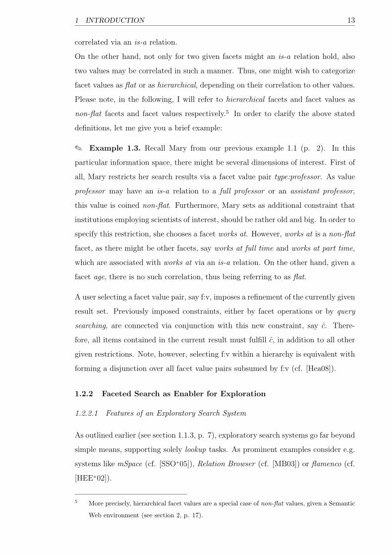
On the other hand, not only for two given facets might an is-a relation hold, also
two values may be correlated in such a manner. Thus, one might wish to categorize
facet values as flat or as hierarchical, depending on their correlation to other values.
Please note, in the following, I will refer to hierarchical facets and facet values as
non-flat facets and facet values respectively.5 In order to clarify the above stated
definitions, let me give you a brief example:
. Example 1.3. Recall Mary from our previous example 1.1 (p. 2). In this
particular information space, there might be several dimensions of interest. First of
all, Mary restricts her search results via a facet value pair type:professor. As value
professor may have an is-a relation to a full professor or an assistant professor,
this value is coined non-flat. Furthermore, Mary sets as additional constraint that
institutions employing scientists of interest, should be rather old and big. In order to
specify this restriction, she chooses a facet works at. However, works at is a non-flat
facet, as there might be other facets, say works at full time and works at part time,
which are associated with works at via an is-a relation. On the other hand, given a
facet age, there is no such correlation, thus being referring to as flat.
A user selecting a facet value pair, say f:v, imposes a refinement of the currently given
result set. Previously imposed constraints, either by facet operations or by query
searching, are connected via conjunction with this new constraint, say c. There-
fore, all items contained in the current result must fulfill c, in addition to all other
given restrictions. Note, however, selecting f:v within a hierarchy is equivalent with
forming a disjunction over all facet value pairs subsumed by f:v (cf. [Hea08]).
1.2.2 Faceted Search as Enabler for Exploration
1.2.2.1 Features of an Exploratory Search System
As outlined earlier (see section 1.1.3, p. 7), exploratory search systems go far beyond
simple means, supporting solely lookup tasks. As prominent examples consider e.g.
systems like mSpace (cf. [SSO+05]), Relation Browser (cf. [MB03]) or flamenco (cf.
[HEE+02]).
5 More precisely, hierarchical facet values are a special case of non-flat values, given a Semantic
Web environment (see section 2, p. 17).

1 INTRODUCTION 14
According to [WR09], advanced systems, such as the above, have to provide a certain
set of features, in order to fulfill high-level information needs. Below, please find
these features outlined in more detail:
(i) Query Formulation & Refinement
A System must enable its users to articulate and instantly refine queries.
(ii) Facets & metadata-based Filtering
Facets need to be present, in order for users to quickly refine and explore a
given result set. Also filtering via document metadata has to be possible.
(iii) Utilize Search Context
Search context, user information and search task information, need to be used
for personalization of the search process.
(iv) Support Visualization
Systems must provide advanced result visualization means, for enabling deci-
sion making and gaining novel insights.
(v) Learning & Understanding
Information has to be visualized and processed in ways making it possible for
users to gain new knowledge and skills.
(vi) User Collaboration
In order to complete high-level information needs, collaboration in a syn-
chronous or asynchronous manner might be necessary.
(vii) History, Workspaces & Updates
Systems have to enable reversion and backtracking of user actions, visualization
of progress updates and storage as well as manipulation of information needed
during the completion of a particular task.
(viii) Task Management
Also, systems must enable multiuser and multisession usage and therefore pro-
vide means of a task management.

1 INTRODUCTION 15
1.2.2.2 Faceted Search as Part of an Exploratory Search System
As briefly described earlier (see section 1.2.2.1, p. 13), exploratory systems need a
set of features to be present, in order to support more advanced search tasks (cf.
[WR09]). One of these features is a faceted interface, as a basis for instant result
set refinement and user exploration of the underlying information space. In the
following, let me explain in more detail, on how a faceted search may contribute to
an exploratory search system.
In compliance with [WR09], “[. . . ] search systems must offer the ability for searchers
to filter result sets by specifying one or more desired attributes of the search results”.
Also, users are often overwhelmed by a given result set and wish to have a meaning-
ful grouping of the result items, in order to deepen their understanding and continue
the search process (cf. [Hea06]). This grouping may be accomplished by using either
clustering techniques or a faceted categorization (cf. [WR09]). According to [Hea06],
faceted categories summarize a given domain of interest, by providing a set of facets
and facet values to users. Thus, allowing them to quickly identify important con-
cepts and deepening their understanding of a given data-space. Furthermore, faceted
search interfaces assist users, when being lost and help getting back on the right
track, via expansion of the result set (cf. [WR09]).
On the other hand, there are also downsides associated with a faceted categoriza-
tion. First of all, many faceted interfaces still depend on manual creation of facet
hierarchies and their associated facet values. Please note, however, there are strong
research efforts on automatic facet hierarchy discovery (see [SH04, DIW05]). Also,
facets may restrict users in their exploration, due to the structural constraints, they
might be imposing (cf. [WR09]).
1.3 Outline of this Paper
Hereafter, I will present a framework for a more browse-able faceted search in a
Semantic Web environment. In contrast to current approaches, which are focused
on efficient query searching strategies, i.e. support for users, in order to issue precise
and specific information needs, rather than enabling them to browse and articulate
fuzzy knowledge. In section 2 (p. 17), I am going to outline a search process, which
allows a fluent interaction between keyword search and browsing. Also, I introduce
definitions for a data, a query as well as a facet model. Continuing in section 3 (p.

1 INTRODUCTION 16
36), again targeting at browse-ability, I will address the problem of vast and unclear
facet ranges. In order to enable users to better understand and access these sets, I
use clustering techniques for decomposing facets in more fine-grained sub-facets. In
section 4 (p. 70), I present a ranking scheme making use of this sub-facet clustering
as well as the individual facet characteristics. Keeping the above goals in mind, these
metrics aim to rank facets high, which support browsing and specification of fuzzy
knowledge, thus are suitable for exploration tasks. In section 5 (p. 91), I discuss
results I obtained from a task-based user study, for comparison of the outlined novel
ranking and clustering approach, with the current state of the art. Finally, in section
6 (p. 99), I present concluding remarks and give the reader a brief overview of future
work, I am planning on pursuing.

Section 2
Faceted Search in a Semantic Web Context
2.1 The Need for a more semantic Web
As briefly outlined in section 1.1.1 (p. 1), nowadays, we are living in an information
age. Efficient data storage as well as access, have become more and more challenging,
with the rapidly increasing amount of content available. However, the current state
of the art for data, or to be more precise, knowledge storage, bears significant flaws.
First, and perhaps most importantly, today data is stored without making its implied
semantics explicit. In other words, while data syntax is machine accessible, data
semantics are only readable for humans. To be more precise, currently, it is up
to the human reader to process a given information and understand its meaning.
Search engines, consider e.g. Yahoo6 or Google7, compensate this lack of intelligence
with IR strategies, trying to reconstruct the before lost semantics. In the long run,
however, it is quite obvious that semantics have to be stored along with their data
and should not be regenerated afterwards (cf. [AvH08, HKRS07]).
A second shortcoming of todays information storage results from its heterogeneity.
It is currently not possible to integrate or reuse given data in any way. For enabling
a more efficient data handling, on the other hand, it is essential to have a common
representation for knowledge (cf. [AvH08, HKRS07]).
Lastly, not all information is stored using an explicit manner. On the contrary, most
information needs are currently fulfilled, not by machines answering a query, but by
users reasoning on an information space. Clearly, this is not a desirable state, since
human reasoning capabilities are generally very limited (cf. [AvH08, HKRS07]).
Please note, a full discussion of the pros and cons of a Semantic Web is beyond the
6 See also http://www.yahoo.com, revised Nov. 2009.
7 See also http://www.google.com, revised Nov. 2009.

2 FACETED SEARCH IN A SEMANTIC WEB CONTEXT 18
limits of this paper. For more details, please see [BLHL01, SBLH06]. Hereafter,
the reader is assumed to have basic knowledge of RDF(S) as well as Semantic Web
technologies in general.
2.2 Semantic Search Process
2.2.1 Search Process - A technical Point of View
In recent years, the amount of data stored, using semantic technologies has increased
drastically. As prominent indicators for more data being represented by means
of ontologies, consider e.g. the increasing usage of languages like RDFa8 or the
Linked Open Data9 initiative. This development enabled a new kind of information
access, providing ways reaching, beyond simple keyword search. Notice, there are
various definitions of semantic search, see e.g. [GMM03, ZYZ+05, CCPC+06]. In
the following, however, semantic search is defined in compliance with [THS09]:
+ Definition 2.1. Semantic Search
Semantic search is defined as an “[. . . ] information access, in which information
needs are addressed by considering the meaning of the user queries and available
resources”, cf. [THS09].
+ Definition 2.2. Semantic Faceted Search
Semantic faceted search, on the other hand, may be defined as semantic search,
employing the faceted search paradigm, in order to enable users to express their
information needs.
In this context, please recall the different information needs as discussed in section
1.1.1 (p. 1). Given data represented via semantic technologies, the question arises,
how to integrate the before introduced faceted search notion, within this new envi-
ronment. However, before discussing an application of faceted search, with respect
to a Semantic Web infrastructure, any further, allow me to first present semantic
search in more detail. According to [THS09], semantic search may be regarded as
a process having the following parts.
8 See also http://w3.org/TR/xhtml-rdfa-primer/, revised Dec. 2009.
9 See also http://esw.w3.org/topic/SweoIG/TaskForces/CommunityProjects/LinkingOpenData,
revised Dec. 2009.
2 FACETED SEARCH IN A SEMANTIC WEB CONTEXT 19
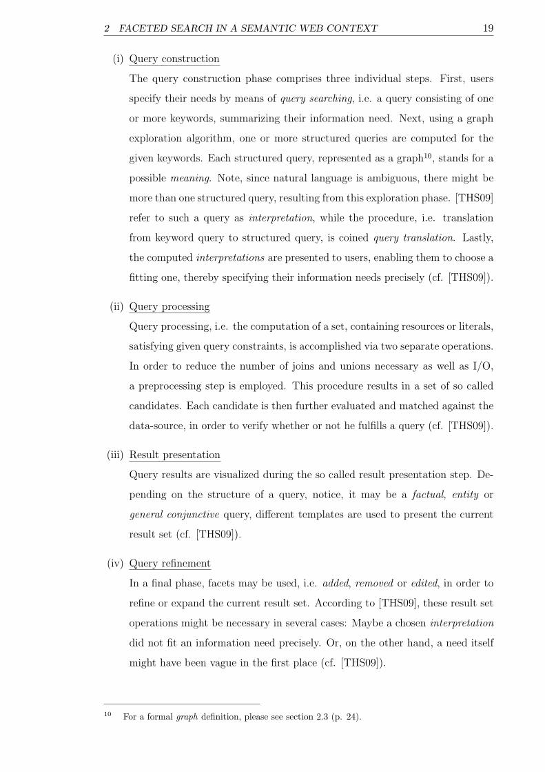
(i) Query construction
The query construction phase comprises three individual steps. First, users
specify their needs by means of query searching, i.e. a query consisting of one
or more keywords, summarizing their information need. Next, using a graph
exploration algorithm, one or more structured queries are computed for the
given keywords. Each structured query, represented as a graph10, stands for a
possible meaning. Note, since natural language is ambiguous, there might be
more than one structured query, resulting from this exploration phase. [THS09]
refer to such a query as interpretation, while the procedure, i.e. translation
from keyword query to structured query, is coined query translation. Lastly,
the computed interpretations are presented to users, enabling them to choose a
fitting one, thereby specifying their information needs precisely (cf. [THS09]).
(ii) Query processing
Query processing, i.e. the computation of a set, containing resources or literals,
satisfying given query constraints, is accomplished via two separate operations.
In order to reduce the number of joins and unions necessary as well as I/O,
a preprocessing step is employed. This procedure results in a set of so called
candidates. Each candidate is then further evaluated and matched against the
data-source, in order to verify whether or not he fulfills a query (cf. [THS09]).
(iii) Result presentation
Query results are visualized during the so called result presentation step. De-
pending on the structure of a query, notice, it may be a factual, entity or
general conjunctive query, different templates are used to present the current
result set (cf. [THS09]).
(iv) Query refinement
In a final phase, facets may be used, i.e. added, removed or edited, in order to
refine or expand the current result set. According to [THS09], these result set
operations might be necessary in several cases: Maybe a chosen interpretation
did not fit an information need precisely. Or, on the other hand, a need itself
might have been vague in the first place (cf. [THS09]).
10 For a formal graph definition, please see section 2.3 (p. 24).

2 FACETED SEARCH IN A SEMANTIC WEB CONTEXT 20
Figure 5: Overall Semantic Search Process (based on [THS09]).
Notice this search process to be summarized in figure 5 (p. 20). Further note,
this description is a rather technical one. More specifically, the main focus lies
on providing a complete overview of necessary steps, internal as well as external,
starting with an unfulfilled and ending with a fulfilled information need. In the
following, I will present another view on the very same search process, addressing
the user-system interactions during a search. Please keep in mind, however, while
having different angles, both views are fully complementary.
Lastly, the reader should be aware that semantic search is a broad research field
and the above stated search process as well as the definitions are intended to give
only a brief overview. For a more detailed introduction to semantic search, please
see [GMM03, Man07, ULL+07].
2.2.2 Search Process - An Information Retrieval Point of View
As mentioned earlier, being complementary to the above description, I would like to
introduce a process view, targeting more at user-system interactions. Please recall,
there are two fundamental IR approaches, namely query searching and browsing (see
section 1.1.2, p. 3). Also remember, in order to enable exploratory search strate-
gies and thereby the fulfillment of higher-level information needs, a combination is
necessary. The hereafter given definition aims at this fluent interaction of query
searching and browsing (based on [HSLY03]).
According to [HSLY03], one may distinguish three different stages during a search

2 FACETED SEARCH IN A SEMANTIC WEB CONTEXT 21
session. First of all, during the so called opening stage, users may familiarize them-
selves with a given information space. Next, there is the middle game, where users
have already narrowed their search space down and intend to further refine the cur-
rent result set via browsing. This phase is followed by what [HSLY03] coined the
end game. Here, a single item of interest, fulfilling an initial information need, is
presented to users. Please also find this process illustrated in figure 7 (p. 23).
In order to combine both IR paradigms in a meaningful manner, one has to make
assumptions, by what means users specify their needs. Please recall, for query
searching a well-defined and very specific information need is necessary. When us-
ing browsing, on the other hand, only vague needs are required. Also reconsider
that query searching is generally less expensive, with respect to time and effort (see
section 1.1.2, p. 3). Given these facts, first of all, I assume users to be aware of
these differences and more importantly, to act in a rational manner. By rational
manner, I mean that users prefer a cheaper path, leading to their item of interest,
over a more expensive one. Thus, without loss of generality, I may have assumptions
as follows:
ó Assumption 2.1.
Specific information needs are always articulated via query searching.
ó Assumption 2.2.
Fuzzy information needs are always entered via browsing.
Given these assumptions, one may combine them as:
ó Assumption 2.3.
First of all, I assume users to be provided with means of query searching as well as
browsing. Also, the reader may think of an information need as an abstract query,
say QNeed. With abstract in this context, I refer to queries being located at some
level between a user need and its machine readable representation. Furthermore, I
see QNeed as a tuple having two elements, say QSNeed and QF
Need with QSNeed resulting
from specific information needs and QFNeed from non-specific or fuzzy needs. Both,
i.e. QSNeed and QF
Need, may be empty. In conclusion, I assume users to articulate
QSNeed via query searching, while needs in QF
Need will be issued applying browsing
strategies.

2 FACETED SEARCH IN A SEMANTIC WEB CONTEXT 22
Please remember in this context also example 1.1 (p. 2). Reconsidering this scenario,
the reader should notice that there are two dimensions of fuzziness11: (i) Users
may only have vague knowledge, with regard to a given underlying domain. E.g.
Mary cannot precisely define the term prestigious, whereas a domain expert would
know that famous computer scientists often won a Turing Award. (ii) Secondly,
users might have vague information, concerning the characteristics of their item of
interest. Mary e.g. is not aware of name or age of any prestigious scientist. Below,
also consider example 2.1 (p. 22), to further clarify assumption 2.3 (p. 21), as well
as the outlined notion of fuzziness.
. Example 2.1. In figure 6 (p. 22), please find the novice computer science
student Mary. Her initial information need was to find famous computer science
researchers and learn more about their work. As shown below, this need may be
represented by queries of different granularity.
Figure 6: Information Need as an abstract Query QNeed
Hereafter, I will further discuss the above mentioned search process model (based
on [HSLY03]). I am going to present each stage as well as the transitions between
the stages in more detail.
11 In the following, fuzzy, vague or unspecific will be used synonymously.
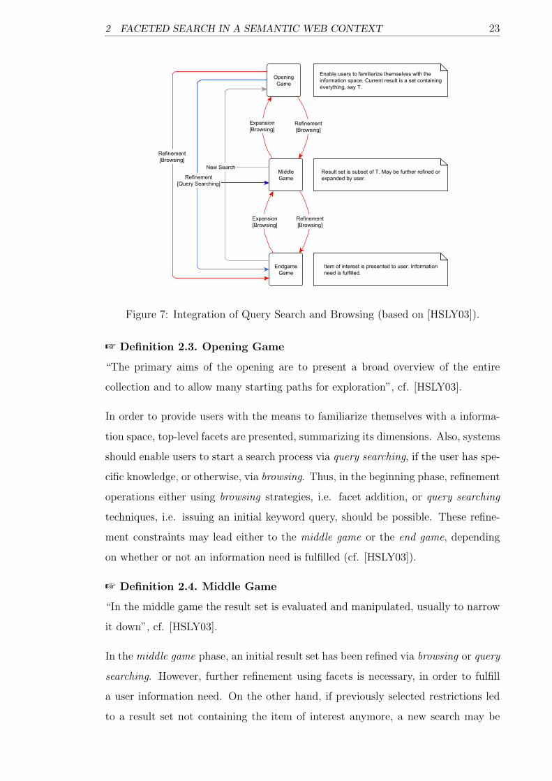
2 FACETED SEARCH IN A SEMANTIC WEB CONTEXT 23
Figure 7: Integration of Query Search and Browsing (based on [HSLY03]).
+ Definition 2.3. Opening Game
“The primary aims of the opening are to present a broad overview of the entire
collection and to allow many starting paths for exploration”, cf. [HSLY03].
In order to provide users with the means to familiarize themselves with a informa-
tion space, top-level facets are presented, summarizing its dimensions. Also, systems
should enable users to start a search process via query searching, if the user has spe-
cific knowledge, or otherwise, via browsing. Thus, in the beginning phase, refinement
operations either using browsing strategies, i.e. facet addition, or query searching
techniques, i.e. issuing an initial keyword query, should be possible. These refine-
ment constraints may lead either to the middle game or the end game, depending
on whether or not an information need is fulfilled (cf. [HSLY03]).
+ Definition 2.4. Middle Game
“In the middle game the result set is evaluated and manipulated, usually to narrow
it down”, cf. [HSLY03].
In the middle game phase, an initial result set has been refined via browsing or query
searching. However, further refinement using facets is necessary, in order to fulfill
a user information need. On the other hand, if previously selected restrictions led
to a result set not containing the item of interest anymore, a new search may be

2 FACETED SEARCH IN A SEMANTIC WEB CONTEXT 24
started or the current result set may be expanded, using facet removal means (cf.
[HSLY03]).
+ Definition 2.5. End Game
“The endgame shows a single selected item in the context of the current query”, cf.
[HSLY03].
Lastly, during the end game, an item of interest has been discovered and is to be
further explored. Also, a new search process may be started or, if related items are
of interest, the result space may be expanded, using facet operations (cf. [HSLY03]).
2.3 Terminology & Definitions
Hereafter, I will first present basic definitions for the underlying data and schema
model, as well as the query model. In a second step, I will introduce definitions
for facets as well as facet values, given a Semantic Web context. Please note, there
are several different definitions for the data, the semantic or the query model, com-
monly used in the literature. I, however, will use these concepts in compliance with
[THS09], as defined below.
2.3.1 Data Model
According to [THS09], the data model or resource space, may be defined as:
+ Definition 2.6. Resource Space
Let SR be the resource space, i.e. is a set of RDF graphs gR = (V R, LR,ER), where
- V R is a finite set of vertices. V R is a disjoint union V RE ⊎ V R
V with E-vertices
V RE (entities) and V-vertices V R
V (data values),
- LR is a finite set of edge labels, subdivided by LR = LRR ⊎ LRA, where LRR are
relation labels and LRA are attribute labels.
- ER is a finite set of edges of the form e(v1, v2) with v1, v2 ∈ V R and e ∈ LR.
Moreover, the following types are distinguished:
- e ∈ LRA (A-edge) iff v1 ∈ V RE and v2 ∈ V R
V ,
- e ∈ LRR (R-edge) iff v1, v2 ∈ V RE ,
- and type, a predefined edge label that denotes the class membership of
an entity (based on [THS09]).
2 FACETED SEARCH IN A SEMANTIC WEB CONTEXT 25
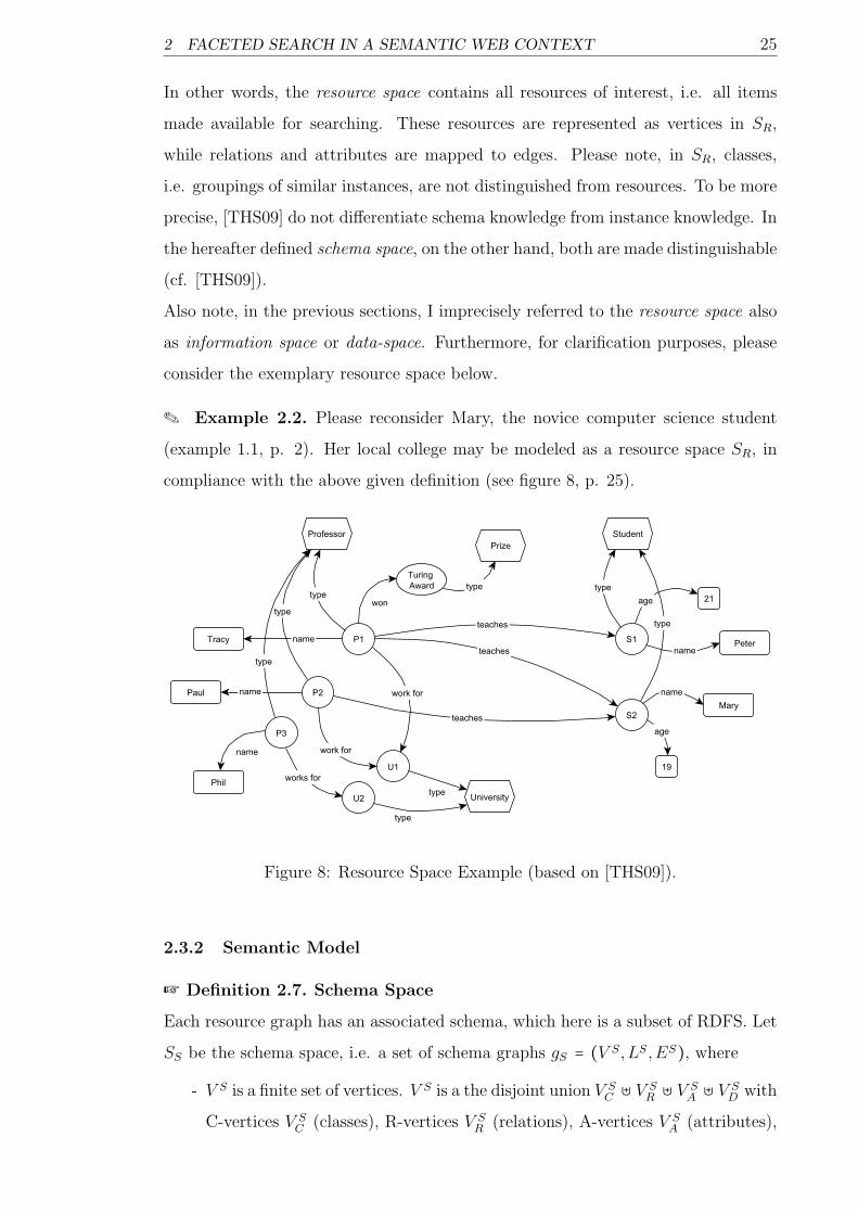
In other words, the resource space contains all resources of interest, i.e. all items
made available for searching. These resources are represented as vertices in SR,
while relations and attributes are mapped to edges. Please note, in SR, classes,
i.e. groupings of similar instances, are not distinguished from resources. To be more
precise, [THS09] do not differentiate schema knowledge from instance knowledge. In
the hereafter defined schema space, on the other hand, both are made distinguishable
(cf. [THS09]).
Also note, in the previous sections, I imprecisely referred to the resource space also
as information space or data-space. Furthermore, for clarification purposes, please
consider the exemplary resource space below.
. Example 2.2. Please reconsider Mary, the novice computer science student
(example 1.1, p. 2). Her local college may be modeled as a resource space SR, in
compliance with the above given definition (see figure 8, p. 25).
Figure 8: Resource Space Example (based on [THS09]).
2.3.2 Semantic Model
+ Definition 2.7. Schema Space
Each resource graph has an associated schema, which here is a subset of RDFS. Let
SS be the schema space, i.e. a set of schema graphs gS = (V S, LS,ES), where
- V S is a finite set of vertices. V S is a the disjoint union V SC ⊎ V S
R ⊎ V SA ⊎ V S
D with
C-vertices V SC (classes), R-vertices V S
R (relations), A-vertices V SA (attributes),

2 FACETED SEARCH IN A SEMANTIC WEB CONTEXT 26
and D-vertices V SD (datatypes).
- LS consists of the labels: subClassOf, domain, range, subPropertyOf.
- ES is a finite set of edges of the form e(v1, v2) with v1, v2 ∈ V S and e ∈ LS,
where
- e = domain iff v1 ∈ V SA ∪ V S
R and v2 ∈ V S
- e = range iff v1 ∈ V SA , v2 ∈ V S
D or v1 ∈ V SR , v2 ∈ V S
C , and
- e = subclassof iff v1, v2 ∈ V SC (based on [THS09]).
. Example 2.3. Continuing the example 2.2 (p. 25), below, please see figure 9
(p. 26) for a schema space associated with Mary’s resource space SR.
Figure 9: Schema Space Example (based on [THS09]).
2.3.3 Query and Result Model
After introducing the resource space SR and schema space SS, in the following I will
focus on the query model. Please recall in this context the above (see section 2.2,
p. 18) outlined search process. Specifically reconsider that an information need,
formulated as keyword query, is mapped to an interpretation. This interpretation is
represented as a so called query graph. In compliance with [THS09], for computing
an interpretation, given a keyword query, three steps are necessary: “(i) Construc-
tion of the query space, (ii) top-k query graph exploration and (iii) query graph
ranking”.
With respect to the scope of this paper (see section 1.3, p. 15), the query graph as
well as its underlying semantic model, i.e. the query space, are of great interest. Fur-
thermore, hereafter, I will define facet operations as a special case of a query graph.

2 FACETED SEARCH IN A SEMANTIC WEB CONTEXT 27
These facet constraints allow users to iteratively construct a query, matching their
information needs (cf. [THS09]). Outlining the computation of an interpretation,
however, exceeds the limits of this paper. The interested reader may see [TWRC09].
2.3.3.1 Query Model
In accordance with [THS09], the query space, i.e. the underlying semantic model of
the query graph, may be given by:
+ Definition 2.8. Query Space
Let SQ(SS,NK) be the query space, comprising keyword matching elements NK
(computed for a keyword query q) and elements of a special schema space, say SS.
SQ consists of the graphs gS(V Q, LQ,EQ), where
- V Q is conceived as the disjoint union V SC ⊎ V S
R ,
- LQ comprises the predefined edge labels subClassOf, domain, range and
subPropertyOf
- EQ is a finite set of edges e(v1, v2) with v1, v2 ∈ V Q and e ∈ LQ (based on
[THS09]).
NK , i.e. elements fulfilling keyword constraints, may be computed via matching
keywords against labels of elements contained in SR. Also note SS being a slightly
modified version of our schema space SS. SS is similar to the above schema space,
however, it does not contain vertices v ∈ VA ⊎ VD, i.e. attributes or datatypes.
Construction of SS seems necessary, as paths in SS end at a datatype vertex and
any edge e(v1, v2), where v1 ∈ VA and v2 ∈ VD, is thus not useful within this context
(cf. [THS09]).
. Example 2.4. Given SR as defined in example 2.2 (p. 25), and SS as defined
in example 2.3 (p. 26). Now, consider as a toy example a keyword query professor
teaches Mary 19, say q. Please see the resulting search space in figure 10 (p. 28),
with elements matching keywords being colored in red.
Finally, a query graph gq for a given query q, is defined as:
+ Definition 2.9. Query Graph
Given SQ = (SS,NK) as query space and K = {k1, . . . , kn} as a set of keywords.
Let f ∶ K ↦ 2VK ⊎EK be a function that maps keywords to sets of corresponding

2 FACETED SEARCH IN A SEMANTIC WEB CONTEXT 28
Figure 10: Search Space Example (based on [THS09]).
graph elements (where V QK , E
QK ⊆ NK). Then, a query graph is a matching subgraph
gq = (Vq, Lq,Eq) with
- Vq ⊆ V SC ⊎ V S
R ⊎ NK ⊎ V QV with V Q
V being a set of variables and
- Lq, Eq comprising elements of SS.
Furthermore, the following constraints have to hold:
- ∀k ∈ K: f(k) ∩ (Vq ∪ Eq) ≠ ∅, i.e. gq contains at least one representative
keyword matching element, for each keyword contained in K, and
- gq is connected, i.e. there exists a path from every graph element to every
other element (based on [THS09]).
Note that there might more than one matching query graph for a given query space.
For finding the best, i.e. top-ranked, k graphs gqi , [THS09] employ a top-k ex-
ploration procedure. Again, for details on the exploration algorithm, please see
[TWRC09]. Hereafter, I assume to have gq given and thus will treat the underlying
algorithm as a black box.
. Example 2.5. Given example 2.2 (p. 25) as resource space, example 2.3 (p. 26)
as schema space and example 2.4 (p. 27) as query space. After the exploration, a
possible query graph is shown in figure 11 (p. 28). Please note, variables are marked
blue and keyword matchings in red.
Figure 11: Query Graph Example (based on [THS09]).

2 FACETED SEARCH IN A SEMANTIC WEB CONTEXT 29
2.3.3.2 Result Model
+ Definition 2.10. Result Space
A result space for a query interpretation gp = (Vq, Lq,Eq) is a set, say SRes, contain-
ing j result graphs gResi = (V Res, LRes,ERes) with i ≤ j. Each gResi = (V Res, LRes,ERes)is a subgraph of one of the resource graphs gR (see definition 2.6, p. 24). Further-
more, each gResi satisfies gp. More precisely, gResi is said to satisfy gp iff
- ERes = Eq, i.e. every edge contained in gq must be contained in gRes,
- LRes = Lq, i.e. labels for these edges have to match,
- ∀ v ∈ Vq /V QV ∶ v ∈ V Res and
- there exists a surjective function h ∶ V RE ↦ V Q
V , so that there is exactly one
mapping V RE ↦ V Q
V , for each v ∈ V RE .
Note, however, the definition of a result space to be depending on a given query graph.
With respect to the chosen interpretation, the result space may vary significantly.
. Example 2.6. Reconsider the earlier examples. For a possible result space,
given the above introduced resource space and query graph, please see figure 12 (p.
30). Notice the coloring to be consistent with the one before.
2.3.3.3 Facet & Facet Value Model
Facet and Facet Value Definitions In the following, I will introduce a facet
model specifically suited for our Semantic Web context. Remember, I see facet
constraints as a special case of a query graph and therefore will use them as means
for specifying an information need.
+ Definition 2.11. Facet & Facet Domain
Given a resource space SR with gR, a result space SRes with gResi and a query graph
gq, the set containing all facets, say F , may be defined as a k-tuple of sets with
F = {Fi}1≤ i≤k and k = ∣V QV ∣. Note that for each vi ∈ V Q
V , there exists a set, say
V REi
⊆ V RE , containing its associated entities. To be more precise, there is an inverse
relation h−1 ∶ V QV ↦ V R
E and V REi
= {v ∈ V RE ∣ v ∈ h−1(vi)} (see definition 2.10, p.
29). Now, let Fi be a set defined as Fi = {e ∈ LR ∣ e(v1,∗) ∈ ER ∧ v1 ∈ V REi}, i.e. Fi
contains all outgoing edge labels of an entity e ∈ VEi . Finally, a facet fi is given by
one element of Fi, i.e. fi corresponds to one e ∈ Fi. Hereafter,b= is used to associate

2 FACETED SEARCH IN A SEMANTIC WEB CONTEXT 30
Figure 12: Result Space Example
a facet with its edge label. Informally speaking, one may say that fi is based on
e ∈ Fi. Note, Fi describes all facets for a given set of entities V REi
, which are mapped
to a variable in the query graph vi. vi is in the following referred to as domain of
facets in Fi. Furthermore notice, the set of all facets, given a resource space SR,
is denoted by FR. Lastly, the reader should be aware that Fj ∈ {Fi}1≤ i≤k do not
necessarily have to be pairwise disjoint, in fact, they might be overlapping.
Note that there are several varying definitions of a facet, given a Semantic Web
context (see [ODD06, SVH07, HMS+05]). The above terminology is most similar to
[ODD06], where facets are informally defined according to RDF triples. In [ODD06]
predicates correspond to facets and their objects are mapped to facet values. How-
ever, there are also significant differences between our definition and the one given
in [ODD06].
First of all, [ODD06] do not distinguish between incoming and outgoing predicates12.
Therefore, both directions may be used as basis for a facet. I, on the other hand,
argue, in accordance with RDF terminology (see e.g. [CK00]) as well as our defini-
12 Note, predicate is used here in compliance with RDF terminology.

2 FACETED SEARCH IN A SEMANTIC WEB CONTEXT 31
tions of a resource space and a schema space, that, given a triple (subject, predicate,
object), the object, in combination with the predicate, specifies the subject and not
the other way around. Thus, I think that only outgoing properties may provide a
meaningful basis for a facet definition. Also, note that our terminology incorporates
the different points of origin facets may have. Given a query graph, every variable
v ∈ V QV may have its own facets associated. This leads to a far more advanced
way of query modifications and thereby enables users to specify their needs more
precisely.
+ Definition 2.12. Facet Value
Given a resource space SR with a graph gR, a result space SRes with gResi , a query
graph gq and facets F = {Fi}1≤ i≤k with k = ∣V QV ∣. For a facet f ∈ Fi ∈ F , there is a
set of associated resources13 Oi(f) = {vj ∈ V R ∣ e(vi, vj) ∈ ER ∧ vi ∈ V REi∧ f b= e}.
Now, facet values may be defined as a set FVi(f) with FVi(f) being a subset of the
power set of Oi(f), i.e. FVi(f) ⊆ P (Oi(f)). Finally, given a facet f , a single facet
value is hereafter denoted by fvi(f) ∈ FVi(f). In the following, the set of all facet
values is referred to as FV R. Furthermore, the reader should be aware that FVi(f)may be pairwise overlapping, with regard to different facet domains vi.
Notice, since facet definitions tend to differ within the literature, other facet value
definitions are also common (see [ODD06, SVH07, HMS+05]). Again, [ODD06] use
the most similar terminology, to the one introduced. Recall, [ODD06] define facets
and facet values respectively, according to RDF triples. Therefore, given a facet f ,
the set of all facet values, i.e. FV∗(f), equals the set O∗(f) as defined above.
I, on the other hand, argue that, in order to truly support exploration (see section
1.1.3, p. 7), not only single facet values are necessary, but also partitions of the
value space. Thus, our definition comprises not solely O∗(⋅), but rather P (O∗(⋅)).Clearly, this goes hand in hand with facet value clustering techniques, taking O∗(⋅)as an input and resulting in a value partitioning. For more details on the actual
algorithms, please see section 3 (p. 36). Furthermore, since I defined facets in a
domain specific manner (see definition 2.11, p. 29), facet values are automatically
also domain specific, allowing users to specify informations needs more accurately.
With respect to the query model, facets, more precisely, facet value pairs f :fv, cor-
respond query predicates. Like predicates, f :fv may be combined via conjunction.
13 Note that using RDF terminology, these resources would be referred to as objects.

2 FACETED SEARCH IN A SEMANTIC WEB CONTEXT 32
More specifically, given a query graph gq = (Vq, Lq,Eq), for each variable vi ∈ V QV
and each fv ∈ FVi(f), a predicate, having a structure e:v with fb= e and v ∈ fv,
may be added to vi in gq. This results in new graphs {giq}i with 1 ≤ i ≤ ∣fv∣. Note,
these {giq}i are independent query graphs, each having an result space associated.14
Furthermore, in a similar manner, a facet value pair may be removed from a current
query graph.
+ Definition 2.13. Facet Value Count
Given a resource space SR with gR, a result space SRes with gResi , a query graph gq
and facets F = {Fi}1≤ i≤k, where k = ∣V QV ∣. I distinguish two different facet value
counts :
(i) Source Count
Given a facet f , the so called source count, say countS, of a facet value fv ∈FV∗(⋅) is defined as: countS(fv) = ∣CS(fv) ∶= {v ∈ V Res ∣∀ v ∈ fv ∶ e(v, v) ∧f
b= e}∣. Note, what I coined source count is known in the literature simply as
count (cf. [Tun09]).
(ii) Value Count
Please reconsider, according to definition 2.12 (p. 31), I essentially define
facet values for a facet f , as an arbitrary set of objects connected via an edge
e ∈ ERes and fb= e. Therefore, I argue that a second count, reflecting the size
of the set, represented by a facet value, is necessary. In conclusion, given a
facet value fv, I define countV as: countV (fv) = ∣CV (fv) ∶= fv∣.
Note that both sets, i.e. CS as well as CV , are defined as mathematical sets, i.e.
each element is only allowed one membership. I will refer to counts associated with
these sets as non-overlapping. However, for ranking purposes (see section 4, p.
70), I extend above defined sets to multisets, say COS and CO
V respectively, thereby
allowing elements to have more than membership. Counts resulting from COS or CO
V ,
I refer to as being overlapping. This differentiation is of particular importance in our
context, since subjects may be mapped to objects15 in a one-to-one, one-to-many,
many-to-one or many-to-many manner. Please see figure 13 (p. 33) for a generic
example.
14 Clearly, depending on giq, its result space may be empty.
15 Note, the terms subject and object are used according to RDF terminology.

2 FACETED SEARCH IN A SEMANTIC WEB CONTEXT 33
Figure 13: Subject to Object Mapping Example
+ Definition 2.14. Given a set of facets F , where F = {Fi}1≤ i≤k. Facet f ′′ ⊑ f ′
(f ′ is said to subsume f ′′) holds iff subPropertyOf(e′′, e′) with e′′b= f ′′ and e′
b= f ′.
. Example 2.7. Continuing our example, please see figure 14 (p. 34) for a facet
model, given our result space. Facets are colored in green, while facet values are
gray or black, depending on whether or not they are contained in the query graph.
Furthermore, there are two facet domains given, say ’1’ for the professors and ’2’ for
the students; both are marked blue. More precisely, facets are given by F = {F1, F2}with F1 ={name, teaches, works for} and F2 ={name, age}. Facet counts are as
follows: countS(S2) = 2, countS(Tracy) = 1, countS(Paul) = 1, countS(U1) = 2,
countS(Mary) = 1, countS(19) = 1 and for all value counts, countV (⋅) = 1 holds.
Facet Characteristics Facets as described in definition 2.11 (p. 29), may be
characterized with respect to different angles. Hereafter, I introduce flat and non-
flat, predefined and non-predefined as well as attribute- and relation-based facets.
Note, however, these characteristics are overlapping in their nature.

2 FACETED SEARCH IN A SEMANTIC WEB CONTEXT 34
Figure 14: Facet Model Example
(i) Flat & Non-Flat Facets
One may distinguish flat or non-hierarchical facets, from facets that are non-
flat or hierarchical. A facet f , is said to be non-flat iff ∃ f ∶ f ⊑ f or f ⊑ f
holds. If, on the other hand, no such f exists, then f is said to be flat or
non-hierarchical.
(ii) Predefined & Non-predefined Facets
With respect to the underlying language used to describe the resource space
SR, as well as the schema space SS, one may differentiate between predefined
and non-predefined relations and facets respectively. Please recall, I assume
RDF(S) as a description language for the data model. Now, given RDF(S),
there are several predefined relations, offering an interesting basis for a facet
definition. Most notably, there is rdf:type, rdf:label and rdfs:seeAlso. rdf:type
associates an instance with its class, enabling a categorization of resources
contained in SR. rdf:label, on the other hand, provides a human-readable name.
Lastly, rdfs:seeAlso links a given resource to other resources, allowing further
exploration. For a complete list of relevant predefined RDF properties, please
see table 1 (p. 102) in the appendix. Note, all other properties, defined during
ontology schema definition, are referred to as non-predefined.

2 FACETED SEARCH IN A SEMANTIC WEB CONTEXT 35
(iii) Attribute-based & Relation-based Facets
Recall, our label set LR comprises LRA, i.e. edges pointing to a data value, as
well as LRR, i.e. edges mapping to other resources. Therefore, I distinguish
facets according to whether they are based on ea ∈ LRA or er ∈ LRR. In the first
case, I refer to facets as attribute-based, in the latter, as relation-based.
Facet Value Characteristics As outlined above, facets may be characterized
with regard to different aspects. In the very same way, one may distinguish facet
values. Hereafter, I define flat and non-flat values respectively.
(i) Flat Value
Recall, according to definition 2.12 (p.31), facet values are given by the power
set of O∗(⋅), formally FV∗(⋅) ⊆ P (O∗(⋅)). Furthermore, depending on whether
this facet is attribute-based or relation-based, O∗(⋅) is either a subset of V RE or
V RV . Thus, a facet value fv is referred to as flat value iff fv ⊆ V R
V .
(ii) Non-Flat Value
On the other hand, a facet value fv is a so called non-flat value iff fv ⊆ V RE ,
i.e. fv comprises entities16.
16 Further note that entities correspond to resources in RDF terminology.

Section 3
Facet Value Construction
3.1 Introduction
Motivation A major goal of faceted search is enabling an exploration of an un-
derlying resource space SR. In order to do so, users are provided with facets, each
having one or more values. However, depending on the facet, it does not make sense
to group every value by its own. Please recall our previously introduced assumption
2.3 (p. 21). Following this thought, users can not be excepted to be able to choose
very specific values, as they do not possess the necessary knowledge. I therefore ar-
gue that O∗ does not provide a useful basis for a facet value definition. In order to be
helpful, a system has to provide meaningful17 subsets of O∗, i.e. FV∗(⋅) ⊆ P (O∗(⋅)).I think these subsets enable users to express their fuzzy knowledge and are thus es-
sential, with regard to our scenario. In contrast, given a vast facet value space,
state of the art systems simple present only top-ranked values and omit all others.18
Clustering, on the other hand, enables a system to visualize the entire value space
and thereby allows users to gain an overview, leading to a far better exploration
and understanding of a resource space. Also, I argue that by applying hierarchical
techniques, specification of fuzzy needs is further supported. More precisely, a hi-
erarchical structure enables users to iteratively articulate vague knowledge via drill
down operations. Thus, besides traditional clustering goals, namely intra- and inter-
cluster similarity, in the following, I will also target browsing support, i.e. what I
coined browse-ability.
Please recall, facet values may be flat, i.e. have no outgoing edges associated, or be
non-flat, i.e. have own relations or attributes (see section 2.3.3.3, p. 35). Hereafter,
17 Note, with meaningful, I refer to sets, sharing a certain pattern proximity.
18 In most cases, systems apply a count-based ranking heuristic.

3 FACET VALUE CONSTRUCTION 37
I distinguish between approaches for constructing non-flat values, on the one hand,
and for flat facet values, on the other. More specifically, I present approaches to
partition O∗, comprising either literals or resources, resulting in FV∗(⋅) ⊆ P (O∗(⋅)).
Problem Definition Before discussing related work, present in the literature, let
me first introduce the clustering terminology applied hereafter as well as a formal
problem definition. Based on [JMF99], I make use of the following concepts:
+ Definition 3.1. Pattern
“A pattern (or feature vector, observation, or datum) x is a single data item used
by the clustering algorithm. It typically consists of a vector of d measurements:
x = {x1, . . . , xd}”, cf. [JMF99].
+ Definition 3.2. Features
“The individual scalar components xi of a pattern x are called features (or at-
tributes)”, cf. [JMF99].
+ Definition 3.3. Class
“A class, in the abstract, refers to a state of nature that governs the pattern gener-
ation process in some cases. More specifically, a class can be viewed as a source of
patterns whose distribution in feature space is governed by a probability density spe-
cific to the class. Clustering techniques attempt to group patterns so that the classes
thereby obtained reflect the different pattern generation processes represented in the
pattern set.”, cf. [JMF99].
+ Definition 3.4. (Hard) Clustering
“Hard clustering techniques assign a class label li to each patterns xi, identifying its
class [. . . ]”, cf. [JMF99].
+ Definition 3.5. Distance Measure
“A distance measure (a specialization of a proximity measure) is a metric (or quasi-
metric) on the feature space used to quantify the similarity of patterns”, cf. [JMF99].
Note, since class is already used in our Semantic Web terminology, I will here-
after refer to this concept simply as cluster. Lastly, below please consider a formal
definition of the problem, I will address throughout this section.
1 Problem 3.1. Facet Value Clustering Problem
Given a facet f for a variable v, its values FVv(f) and a dissimilarity function

3 FACET VALUE CONSTRUCTION 38
d, this problem consists of finding a partitioning of FVv(f), so that d, the browsing
paradigm as well as the current result set are taken into consideration and associated
goals are met.
Components of a Clustering Task In accordance with [JD88], a typical clus-
tering process consists of parts, as briefly outline below:
(i) Pattern Representation
During this first step, the number of clusters and patterns, as well as the type,
number and scale of features, which may be used by an algorithm later on, is
specified. Optionally, a subset containing only the most effective features may
be selected, during the so called feature selection. Furthermore, features might
be transformed, via the feature selection, in order to produce novel and more
efficient features (cf. [JD88, JMF99]).
(ii) Pattern Proximity
The proximity of a given pair of patterns is often defined by means of a distance
function. E.g. given a vector space, such a distance may be estimated in
compliance with the well-known Euclidean distance. However, notice, there are
several ways introduced in the literature, addressing this problem (cf. [JD88,
JMF99]).
(iii) Clustering
Depending on the actual algorithm, a grouping, i.e. a mapping of a pattern to a
cluster, may vary significantly. A set patterns might be divided into partitions,
i.e. each pattern is associated with exactly one cluster, resulting in a so called
hard clustering. On the other hand, in case of a fuzzy clustering, an algorithm
may assign one pattern to several different clusters (cf. [JD88, JMF99]). For
further clustering variances, please see [JMF99].
(iv) Data Abstraction�
During the data abstraction phase, a dataset is represented in an easy and
compact manner. Note, easy in this context is used either with respect to
machine or human readability (cf. [JD88, JMF99]).
(v) Assessment of Output�
Assessment of output refers to a cluster validity analysis. It is intended to

3 FACET VALUE CONSTRUCTION 39
determine whether or not a given clustering algorithm produces a meaning-
ful output. However, in many cases a very specific and subjective notion of
optimality is used (cf. [JD88, JMF99]).
Note � to mark optional steps. Please see also figure 15 (p. 39), summarizing the
above outlined steps.
Figure 15: Components of a Clustering Task (based on [JMF99])
Clustering Intentions w.r.t. our Faceted Search Context Data clustering
is a quite popular research area, where a lot of work has been done. However, our
context is in some sense different, from those of other applications. Thus, before
looking at related work, I would like to first describe our goals, I wish to accomplish,
explicit.
- Strong intra-cluster similarity�
Clearly, I wish entities contained in one cluster to have a strong sense of
similarity, with respect to some predefined measure (see also [JD88]).
- Strong inter-cluster dissimilarity�
Also, I want the resulting clusters to have, in compliance with the same mea-
sure, a weak similarity in-between each other (see also [JD88]).
- Support of fuzzy knowledge�
With regard to user knowledge and an information needs, I intend an algorithm
to construct few clusters, in the best case, being approximately of equal size.
By doing so, I minimize the amount of information necessary, in order to make
a decision, given a set of facet values.

3 FACET VALUE CONSTRUCTION 40
- Support of partial knowledge�
Lastly, I also wish an algorithm to address users on an individual basis, thereby
supporting their, likely to be partial, knowledge. More precisely, users should
be involved in early stages of the process and resulting clusters should reflect
user knowledge the best way possible.
Please notice the former two aspects, marked by �, to represent common clustering
goals. Both intend for a clustering algorithm to produce, with respect to a given
similarity measure, meaningful groupings. However, the latter two, labeled with
�, directly follow the previous assumption 2.3 (p. 21). Recall, I assume users to
only issue information needs contained in QFNeed, i.e. fuzzy and unspecific needs, via
browsing.
Furthermore note, the concept of similarity here is used in a very abstract manner.
In particular, I do not assume a specific similarity function at this point in time. The
notion of similarity may be substantiated, using intuitions by [Lin98], as outlined
below:
- “The similarity between A and B is related to their commonality. The more
commonality they share, the more similar they are.”, cf. [Lin98].
- “The similarity between A and B is related to the differences between them.
The more differences they have, the less similar they are.”, cf. [Lin98].
- “The maximum similarity between A and B is reached when A and B are
identical, no matter how much commonality they share.”, cf. [Lin98].
Notice A and B to represent abstract entities to be compared.
3.2 Related Work
3.2.1 Overview
Please recall, I initially defined facet values, i.e. FV∗(⋅), as a subset of P (O∗(⋅)).Therefore, with respect to clustering strategies, I wish to distinguish between facet
values being a set comprising resources or comprising literals. I argue that this dif-
ferentiation is necessary, since I intend to group similar items together. However,
resources and literals differ heavily, with regard to their structure. Recall, while

3 FACET VALUE CONSTRUCTION 41
literals are essentially flat values, typed according to XML schema, resources repre-
sent entities, having properties to other entities, or attributes, providing a further
characterization.
In the following, let me first present related work for the clustering of resources.
Afterwards, I will introduce other works, which may be used for grouping literals.
However, as I will show, those techniques suffer from significant shortcomings, given
our specific faceted search scenario. Please note, sometimes in the literature pattern
proximity is described by means of a similarity function, while other approaches
represent proximity via a distance measure. In the former case, similar patterns are
assigned higher values, while dissimilar ones are associated with lower numbers. In
the latter case, on the other hand, it is simply the other way around.
3.2.2 Clustering Approaches for Resources
Before looking at approaches, providing a distance measurement for RDF instances,
I wish to point out an issue addressed by [GEP08]. In their work, they argue that
defining a RDF instance in this context is a non-trivial problem. In other words,
given a resource space, the question arises, what constitutes a RDF instance, i.e.:
Where does one instance end and another begins? [GEP08] refer to this problem
as instance extraction. According to their work, there are several ways on how to
define an instance in a clustering context:
(i) Immediate Properties
[GEP08] argue that one solution would be, to only consider immediate prop-
erties to be relevant for a given resource, say r. However, they further outline
that, while being a straight-forward solution, it is also the most discriminative
one. Applying this approach, much important information concerning r could
be lost (cf. [GEP08]).
(ii) Concise Bounded Description
A more sophisticated approach, on the other hand, may wish to also consider
the graph structure as well as the node types (cf. [GEP08]). Concise Bounded
Description (CBD) e.g., uses a recursive algorithm for instance extraction.
Given an instance, say r, CBD takes r itself, its immediate properties and
recursively all properties, if the associated object is a blank node (cf. [Sti05]).
Another variant of this approach, would be, to also consider incoming edges

3 FACET VALUE CONSTRUCTION 42
to be relevant for r (cf. [GEP08]). However, again, [GEP08] also outline
shortcomings associated with this approach. More precisely, they argue that
CBD, since it is strongly depending on blank nodes, is not truly independent
from an underlying domain (cf. [GEP08]).
(iii) Depth-Limited Crawling
In compliance with [GEP08], another approach would be, to limit the subgraph
associated with a resource in question, by restricting the edge distance to a
given threshold value. In contrast to CBD, so [GEP08] argue, this approach
has the advantage, to be completely domain independent, since it does not rely
on specific node types (cf. [GEP08]).
To my knowledge, approaches for clustering RDF instance data may be categorized
with respect to three different angles. On a side note, the reader should notice that
there is currently much attention in the Semantic Web community, especially in the
area of ontology alignment, on measuring entity similarity at schema level. However,
hereafter, let me briefly introduce grouped approaches, targeting instance data.
(i) Vector Space Based Similarity
On the one hand, instances, represented as a RDF graph, could be projected
into a vector space model. Therefore, all distance measures applicable in this
traditional representation, may also be employed here. Obviously, the ques-
tions arises, how to transform resources into a high-dimensional projection.
One solution for this problem is proposed in [GEP08]. Here, the authors argue
that a simply mapping of RDF properties, to dimensions in a vector space is
not sufficient. Thus, they present a rather different method. First, given a
root node X and a graph G, [GEP08] introduce a notion of reachability as:
reachable(X,G) = {n ∣ (x, p, n) ∈ G} ∪ {n′ ∣n′ ∈ RG(n)}. Furthermore, with
shortestPath(R,X,G) denoting the shortest path from a given node R to a
node X in G, they define a feature vector for an instance, say n, as:
FV (n) = {shortestPath(Rn, x,Gn) ∣x ∈ reachable(Rn,G)} (3.1)
Now, they introduce the feature vector for a set of instances as union over all
individual vector sets.

3 FACET VALUE CONSTRUCTION 43
(ii) General Graph Based Similarity
Another perspective would be, to see RDF instance data simply as a graph,
without having additional semantic information. Given this assumption, many
existing distances measures, intended for node comparison in graphs, would be
applicable. Consider e.g. work done in [MGL00], where the authors com-
pare so called conceptual graphs. Note conceptual graphs to be quite sim-
ilar to RDF data, thus providing a good example for potentially suitable
metrics. Conceptual graphs comprise nodes standing for attributes, events
or entities as well as nodes being relations, associating two given nodes (cf.
[Sow84, Sow00]). In accordance with [Sow84, Sow00], a distance measure be-
tween two graphs, say G1 and G2, may be defined, with respect to a so called
overlap graph GC = G1 ∩ G2. To be more precise, GC contains overlap-
ping concept nodes as well as overlapping relation nodes. In a second step,
so [Sow84, Sow00] continue, a similarity value may be derived from GC , by
computing a combination of two different measures, namely the conceptual
similarity and the relational similarity. While the former estimates the degree
of similarity between concepts and actions in both graphs, the latter value
measures the similarity of concept interrelations, i.e. information about con-
cepts (cf. [Sow84, Sow00]). Please note these metrics to have been adopted to
RDF data, see [GEP04, GEP08]. Further note, there is much interesting work
present in the literature, for a survey on graph clustering see [Sch07].
(iii) Ontology Based Similarity
There has been a lot of work done on similarity measures in the context of ontol-
ogy alignment. Generally, these metrics rely strongly on rich semantic schema
data and, while obviously also working on graph structures, may therefore be
distinguished from the above mentioned graph clustering algorithms. Summa-
rizing these works goes clearly beyond the limits of this paper. For surveys
providing such an overview, please see e.g. [SE05, CSH06, KS03]. In order to
make it clearer to the reader, what kind of algorithms I subsume under this
category, allow me to briefly outline one approach by [MZ02], focusing solely
on instance data.
According to [MZ02], a similarity measure for resources may be defined with
regard to three aspects, namely:

3 FACET VALUE CONSTRUCTION 44
(a) Taxonomy Similarity (TS)
The taxonomy similarity value refers to the closeness of two instances, with
respect to their associated concepts and their positioning in the taxonomy.
More specifically, two concepts are compared by the number of common
super-classes. The bigger this overlap is, the more similar two concepts,
thus also their instances, are assumed to be (cf. [MZ02]).
(b) Relational Similarity (RS)
On the other hand, resources may be associated with further entities and
literals via incoming and outgoing edges respectively. Using a second mea-
sure, [MZ02] compare two given resources, say r1 and r2, with regard to
their associated entities. The authors assume r1 and r2 to be similar, if
they share relations to the same or similar resources. Note, this similarity
notion is recursively defined, thus, for avoiding cycles, a maximum depth
threshold is applied (cf. [MZ02]).
(c) Attribute Similarity (AS)
Lastly, following the above outlined thought, [MZ02] define an attribute
similarity, as the similarity of literals connected to the resources in ques-
tion. Obviously, since essentially being data values, such an estimation
may easily be computed, using traditional similarity measures, depending
on the literal type (cf. [MZ02]).
Finally, using the introduced similarity notions as well as given weights, say t,
r and s respectively, [MZ02] define the similarity of r1 and r2 as:
sim(r1, r2) = t ⋅ TS(r1, r2) + r ⋅ RS(r1, r2) + a ⋅ AS(r1, r2)t + r + a (3.2)
Applying our instance definition as well as the described similarity measures, a
specific clustering algorithm may be employed. Note, in recent years, there has
been great interest in clustering, thus, a rich selection of techniques is available. One
commonly used approach, however, I will introduce as an example, is hierarchical
clustering. Given a set of n patterns, an agglomerative variant of a hierarchical
strategy, may be briefly described as (cf. [JMF99]):
- Compute Proximity Matrix
In a first step, each pattern is regarded as its own cluster. For these clusters, a

3 FACET VALUE CONSTRUCTION 45
so called proximity (n×n) - matrix, containing similarity values between every
cluster combination possible, is initially computed.
- Merge Clusters
During a second step, the two most similar clusters, with respect to a given
similarity function, are chosen and merged.
- Update Proximity Matrix
Now, for the reduced set of clusters, the proximity matrix is updated. Step
two and three are repeated, until only one single cluster remains.
Note, hierarchical clustering techniques are often based on single-link (see [SS73])
or complete-link (see [Kin67]) intuitions. However, a comparison of techniques cur-
rently present, is not within scope of this paper. For further details, please see
[JMF99, XW05].
3.2.3 Clustering Approaches for Literals
After the above provided overview of existing approaches for comparing resources,
in the following, I give the reader a survey of clustering techniques and similarity
measures concerning literals. Due to the fact that clustering is a topic of interest
for a vast community, there have been many approaches presented in the literature
for handling literals, i.e. data values (cf. [JMF99, XW05]).
Please recall, given a RDF data-source, one may have to deal with different types
of literals, subsumed under different feature categories. In compliance with [GD92],
features may be distinguished as follows:
(i) Quantitative features
- Continuous values, e.g. weight.
- Discrete values, e.g. number of inhabitants.
- Interval values, e.g. duration time.
(ii) Qualitative features
- Nominal (unordered), e.g. name.
- Ordinal (ordered), e.g. grade.
- Combinational, e.g. student to grade relation (name, grade).

3 FACET VALUE CONSTRUCTION 46
Now, depending on the associated feature category of data values in question, there
might be different similarity measures suitable (cf. [JMF99, XW05]). In the fol-
lowing, I will present exemplary measures for quantitative as well as qualitative
features:
(i) Quantitative features
Since continuous features are quite common in real-world data, allow me to
use these values as representatives for quantitative features in general. How-
ever, even with this restriction, there are still a number of popular measures
applicable. Below please find two well-known distance metrics, namely the
Minkowski as well as the Mahalanobis metric.
- Minkowski Metric
The Minkowski metric may be defined for two given pattern, say xi and
xj, as:
dp(xi, xj) = (d
∑k =1
∣xi,k − xj,k∣p)1/p = ∥xi − xj∥p (3.3)
Note the well-known Euclidean distance metric for p = 2, to be variant
of equation 3.3 (p. 46) (cf. [JMF99]). For an application of this norm,
see e.g. [HBH00].
- Mahalanobis Metric
Furthermore, two continuous features may be correlated, thereby influenc-
ing the similarity measure between a given set of patterns. This problem
is addressed by the Mahalanobis metric. With xi and xj being patterns,
a similarity estimation is calculated as:
dM(xi, xj) = (xi − xj) ⋅−1
∑xi − xjT (3.4)
where ∑ refers to the sample covariance matrix. Note dM(⋅, ⋅) to use
weights, based on variances and pairwise linear correlations of the associ-
ated features (cf. [JMF99]). For an exemplary implementation, consider
e.g. [MJ96].
(ii) Qualitative features
With respect to qualitative features, there is again a rich selection of mea-

3 FACET VALUE CONSTRUCTION 47
sures available in the literature. Thus, I will use strings as a common value
representing this category. Note strings to be considered as a nominal feature.
- Edit-distance-based measures
A well-known approach for computing the distance between two given strings,
is the so called edit distance. Approaches using this technique, a dissimilarity
score is based on edit operations necessary, in oder to transform one of the
given strings, say t1, into the other, say t2. A simple algorithm employing
this strategy is the Levenshtein distance. It is defined as the minimal amount
of insertion, deletion or substitution operations, needed to rewrite t1 as t2
(cf. [Lev65]). Other common approaches include the Hamming distance (see
[SK83]) or the Episode distance (see [DFG+97]).
- Token-based measures
Besides using edit operations as a basis for a similarity measure, one could
also argue that strings may be regarded as two multisets of letters, so called
tokens. Probably the most simple representative in this context is the Jaccard
similarity, first defined in [Jac12], as:
dJ(xi, xj) = 1 − ∣xi ∩ xj ∣∣xi ∪ xj ∣
(3.5)
Note, another well-known approach falling under this category is e.g. the
cosine similarity (cf. [CRF03]).
Furthermore note the presented similarity intuitions to be only a very short sum-
mary, which is clearly not intended to be complete. For a more detailed overview,
please consider surveys present in the literature, see e.g. [JMF99, XW05]. For fur-
ther string metrics, on the other hand, consider [CRF03, Nav01].
With respect to the actual clustering algorithm, the above mentioned techniques
may also be applied, given data values. Again, a detailed discussion is not within
the scope of this paper, please see [JMF99, XW05] for further information.
3.2.4 Contribution
As mentioned earlier, facet values may either be based on literals or based on re-
sources. Thus, with regard to a faceted search application, one is in need of two al-
3 FACET VALUE CONSTRUCTION 48
gorithms, the former for clustering literals, while the latter is applicable for resource-
based values.
Concerning the first problem, i.e. literal clustering, I will present traditional simi-
larity measures, depending on the type of a particular range. More precisely, as a
clustering technique, I apply a well-known hierarchical, divisive clustering approach.
Thereby, I enable users to drill down into a set of values, depending on their indi-
vidual knowledge. In other words, I allow users to issue fuzzy knowledge and thus
fulfill the earlier stated intuitions.
However, I see the main contribution in my solution for the latter task, namely the
clustering of resources. While the above introduced works mainly target intra- and
inter-cluster similarity, I think that, with regard to our use case, further goals need
to be taken into consideration. Please recall the above presented additional intu-
itions to be (i) support of partial knowledge as well as (ii) support of fuzzy knowledge.
Remember those to follow directly from our previous assumptions, concerning the
search process and the user knowledge (see assumption 2.3, p. 21). Given these
extra goals and their background, it becomes obvious that the feature selection step
is a key aspect within this context. With respect to the algorithm itself, I argue
that resources may be regarded as abstract entities, being described by their out-
going properties, i.e. by their relations and attributes. In other words, resources to
be clustered, may simply be seen as a set of entities, which is characterized by its
facets. I therefore conclude that facets should be treated as features. Each property
and facet respectively, describes its associated instance, thus providing a suitable
basis for clustering. Second, I argue that due to the partial knowledge, the feature
selection phase is crucial and has to be controlled solely by an individual user. More
specifically, users should be enabled to choose a facet, which they have knowledge
about, resulting in a system grouping associated resources entirely with respect to
this feature. Notice, however, if the selected facet is a based on a relation, its range
will contain resources, which in turn will be described and clustered in accordance
with their facets. By applying such a strategy, as the evaluation will show, highly
complex queries may be constructed via simple faceted search interactions. In other
words, I argue that clustering, given a faceted search system, should essentially boil
down to a feature selection, i.e. a facet ranking problem. Let me emphasize that
this way, complex user information needs may be addressed, while no additional
paradigms are necessary.

3 FACET VALUE CONSTRUCTION 49
3.3 Literal Clustering
3.3.1 Overview
In a first step, I will define dissimilarity metrics and a clustering technique with
regard to literals. Recall, by doing so, I establish the necessary partitioning of O∗,
in order to construct FV∗(⋅) ⊆ P (O∗(⋅)).As mentioned earlier, a clustering approach and, in particular, a similarity mea-
sure to be applied, for a given set of literals, depends on their assigned type. Also,
please recall that I assume a data-source to be represented by RDF(S). However,
given this framework, there are no built-in datatypes (cf. [MM04]). More specif-
ically, datatypes are identified by a Uniform Resource Identifier (URI), linking to
an externally described concept.19 These type concepts are then defined using the
Extensible Markup Language (XML) Schema framework (cf. [MM04]).
In compliance with [MM04], a datatype may be defined as:
+ Definition 3.6. XML-S Datatype
“In this specification, a datatype is a 3-tuple, consisting of a) a set of distinct values,
called its value space, b) a set of lexical representations, called its lexical space, and
c) a set of facets that characterize properties of the value space, individual values
or lexical items”, cf. [BM04].
With respect to our context, the former two are of particular interest. [BM04] define
these concepts as outlined below:
(i) Value Space
“A value space is the set of values for a given datatype. Each value in the value
space of a datatype is denoted by one or more literals in its lexical space”, cf.
[BM04].
(ii) Lexical Space
The so called lexical space comprises a set of strings, being used to represent
values contained in a value space. More precisely, only elements of a given
lexical space, may be used as representatives for their corresponding elements
in the value space (cf. [BM04]).
19 Note, rdf:XMLLiteral to be an exception of this rule. RDF(S) makes use of this built-in
datatype in order to express XML content as a literal value (cf. [MM04]).

3 FACET VALUE CONSTRUCTION 50
(iii) Lexical-to-value Mapping
Clearly, after defining a lexical as well as a value space, a relation between
these two sets is necessary. To be more precise, such a mapping specifies, which
element in the values space, a given string contained in the lexical space, is
associated with (cf. [BM04]).
For further information concerning the RDF datatype concept or related issues,
please see [MM04]. However, with this background knowledge, let us take a closer
look at the actual datatypes being defined using XML Schema. According to [BM04],
one may distinguish predefined, so called primitive, from non-predefined, i.e. derived,
datatypes.
+ Definition 3.7. Primitive Datatypes
Datatypes, which are not defined on basis of other existing types, may be referred
to as being primitive (cf. [BM04]).
+ Definition 3.8. Derived Datatypes
On the other hand, if a datatype is defined by means of other types, it is coined
derived (cf. [BM04]).
Clearly, covering all possible datatypes by a similarity measures is not possible.
Thus, I will focus solely on common primitive types. However, please note this defi-
nitions to be based on well-known metrics and easily expandable to cover additional
types, if necessary. More precisely, hereafter, I introduce measures for decimal, float
and double, string, time as well as date. For a complete hierarchy of primitive
datatypes present in XML Schema, please see figure 23 (p.103). By means of these
metrics, I then apply a traditional, however slightly adapted, divisive hierarchical
clustering technique.
3.3.2 Definition of a suitable Similarity Measure
In a similar manner, as in the previous section, I first will define type-specific simi-
larity measures. Then, during a second step, I will introduce a clustering technique,
making use of these metrics.

3 FACET VALUE CONSTRUCTION 51
3.3.2.1 Similarity Notion for a single Value
Please remember that facet values are defined as FV∗(⋅) ⊆ P (O∗(⋅)) (see definition
2.12, p. 31). In other words, values I intend to compare are generally sets, each
containing one or more literals. Thus, first of all, let me define a similarity notion
with respect to literals, i.e. single values. Afterwards, I will extend this notion to
also cover sets of literals, i.e. values contained in FV∗(⋅).
XML-Schema Type String In accordance with [BM04], a string in this context
may be seen as:
+ Definition 3.9. String
“The string datatype represents character strings in XML. The value space of string
is the set of finite-length sequences of characters [. . . ]. A character is an atomic unit
of communication; it is not further specified except to note that every character
has a corresponding Universal Character Set code point, which is an integer.”, cf.
[BM04].
Please note that literals being typed as strings are flat, i.e. they only have one feature
associated. Recall, one objective for clustering to be the support of fuzzy knowledge.
In order for users, however, to issue their unspecific knowledge and information needs
respectively, clusters need to be as intuitive and as self-explanatory as possible. On
the other hand, a very well-known way of sorting strings, is given by their lexical
order. With respect to our string distance, I therefore argue that an edit-based
approach may suffice, however, editing costs should be based on the lexicographic
distance between the associated letters. Using such an approach, given two literals,
say s1 and s2, a similarity value would be correlated with their lexical positioning in
a given alphabet, say Σ. Following this thought, a distance between s1 and s2 may
be written as:
disa(s1, s2) =h
∑i=1
⎧⎪⎪⎪⎪⎨⎪⎪⎪⎪⎩
0 if s1(i) = s2(i)
σ−i(ρ(s2(i)) + ρ(s1(i))) otherwise
+⎧⎪⎪⎪⎪⎨⎪⎪⎪⎪⎩
∑∣s2∣j = ∣s1∣ σ−jρ(s2(j)) if ∣s1∣ ≤ ∣s2∣
∑∣s1∣k = ∣s2∣ σ−kρ(s1(k)) otherwise
(3.6)

3 FACET VALUE CONSTRUCTION 52
with h = min{∣s1∣, ∣s2∣}, σ = ∣Σ∣ standing for the size of the alphabet used, s∗(j)referring to the jth character in string s∗ and ρ being a relation, mapping characters
to their lexical position in Σ.
Note that by employing this metric in combination with an hierarchical strategy, the
cluster representation problem may easily be addressed. More precisely, one might
simply use an interval-like naming scheme, i.e. visualize a given cluster by its left
and right border value.
XML-Schema Basic numerical Types As mentioned earlier, most common
numerical types to accrue in real-world data, I think to be decimal, float or double.
Notice that these types are also the most basic ones, according to the hierarchy
defined in [BM04] (see figure 23, p. 103). Further note the below defined measure
to be intended to be generic. Thus, if provided with more specific types, e.g. a
positiveInteger, measures may easily be adapted. However, before discussing our
similarity notion any further, allow me to first outline how decimal, float and double,
may be defined in compliance with [BM04]:
+ Definition 3.10. Decimal
“Decimal represents a subset of the real numbers, which can be represented by
decimal numerals. The value space of decimal is the set of numbers that can be
obtained by multiplying an integer by a non-positive power of ten, i.e., expressible
as i × 10−n where i and n are integers and n ≥ 0. [. . . ] The order-relation on decimal
is the order relation on real numbers, restricted to this subset.”, cf. [BM04].
+ Definition 3.11. Float
“Float is patterned after the IEEE single-precision 32-bit floating point type [. . . ].
The basic value space of float consists of the values m × 2e, where m is an integer
whose absolute value is less than 224, and e is an integer between −149 and 104,
inclusive. [. . . ] The order-relation on float is: x ≤ y iff y − x is positive for x and y
in the value space. [. . . ]”, cf. [BM04].
+ Definition 3.12. Double
“The double datatype is patterned after the IEEE double-precision 64-bit floating
point type [. . . ]. The basic value space of double consists of the values m × 2e, where
m is an integer whose absolute value is less than 253, and e is an integer between
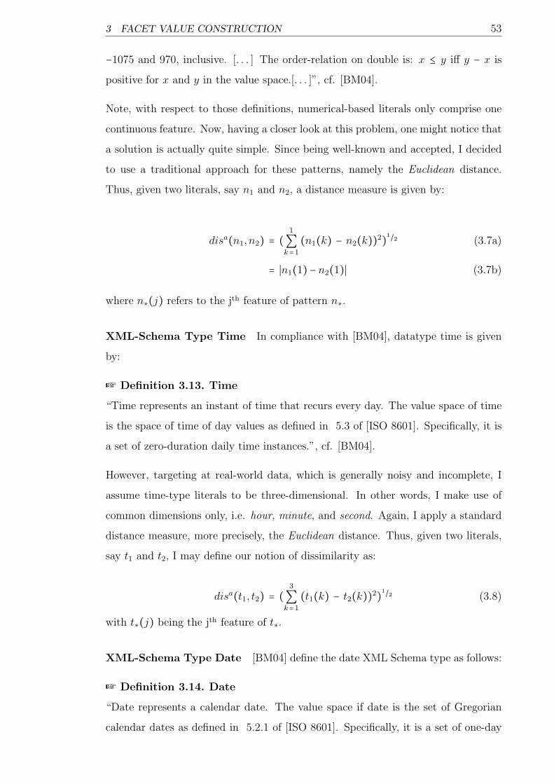
3 FACET VALUE CONSTRUCTION 53
−1075 and 970, inclusive. [. . . ] The order-relation on double is: x ≤ y iff y − x is
positive for x and y in the value space.[. . . ]”, cf. [BM04].
Note, with respect to those definitions, numerical-based literals only comprise one
continuous feature. Now, having a closer look at this problem, one might notice that
a solution is actually quite simple. Since being well-known and accepted, I decided
to use a traditional approach for these patterns, namely the Euclidean distance.
Thus, given two literals, say n1 and n2, a distance measure is given by:
disa(n1, n2) = (1
∑k =1
(n1(k) − n2(k))2)1/2 (3.7a)
= ∣n1(1) − n2(1)∣ (3.7b)
where n∗(j) refers to the jth feature of pattern n∗.
XML-Schema Type Time In compliance with [BM04], datatype time is given
by:
+ Definition 3.13. Time
“Time represents an instant of time that recurs every day. The value space of time
is the space of time of day values as defined in 5.3 of [ISO 8601]. Specifically, it is
a set of zero-duration daily time instances.”, cf. [BM04].
However, targeting at real-world data, which is generally noisy and incomplete, I
assume time-type literals to be three-dimensional. In other words, I make use of
common dimensions only, i.e. hour, minute, and second. Again, I apply a standard
distance measure, more precisely, the Euclidean distance. Thus, given two literals,
say t1 and t2, I may define our notion of dissimilarity as:
disa(t1, t2) = (3
∑k =1
(t1(k) − t2(k))2)1/2 (3.8)
with t∗(j) being the jth feature of t∗.
XML-Schema Type Date [BM04] define the date XML Schema type as follows:
+ Definition 3.14. Date
“Date represents a calendar date. The value space if date is the set of Gregorian
calendar dates as defined in 5.2.1 of [ISO 8601]. Specifically, it is a set of one-day

3 FACET VALUE CONSTRUCTION 54
long, non-periodic instances [. . . ], independent of how many hours this day has.”,
cf. [BM04].
Note, just like the above introduced time type, date comprises several dimensions
or features. However, I again argue that in most applications noisy and incomplete
data is being used. Therefore, I only expect the most common features, i.e. year,
month and day, to be present. Given two dates, say d1 and d2, this leads to a similar
problem as before, so I may apply the Euclidean distance notion, resulting in:
disa(d1, d2) = (3
∑k =1
(d1(k) − d2(k))2)1/2 (3.9)
where d∗(j) stands for the jth feature of d∗.
3.3.2.2 Similarity Notion for Value Sets
In the above section, I outlined how similarity may be defined for single literals.
However, when considering sets, containing more than one literal, one may need to
extend this notion. For clarification purposes, please consider example 3.1 (p. 54).
. Example 3.1. Please find figure 16 (p. 54) presenting nine clusters. Consider
e.g. S, being one big cluster, containing three singleton sets, namely {Si}i ∈{1,2,3}.Furthermore, a second large cluster, say T , is given, comprising again singleton sets,
i.e. {Tj}j ∈{1,...,4}. Note that a similarity, or to be more accurate, a dissimilarity
value, between any of the singleton sets in S or in T may be computed as discussed
earlier. However, the question arises, how a similarity between the big clusters, i.e.
S and T , might be defined.
Figure 16: Generic Example for a Similarity Notion w.r.t. Sets

3 FACET VALUE CONSTRUCTION 55
Clearly, this problem is well-known in the literature and various solutions would
be applicable. However, hereafter, allow me to briefly describe two traditional ap-
proaches, which could be easily integrated.
(i) Single-Link
According to [SS73], a distance between two given clusters, say c1 and c2, may
be described as minimum distance value of all distances, between a pattern
contained c1, while the other element being in c2.
(ii) Complete-Link
On the contrary, [Kin67] argue that the dissimilarity of c1 and c2, may be rep-
resented as maximum value of all dissimilarities, between a pattern contained
c1 and one in c2.
Clearly, other known solutions may also be employed here (see e.g. [JMF99, XW05]).
However, as I will show in the next section, with respect to the clustering technique
applied, a single-link strategy makes the most sense.
3.3.3 Hierarchical Clustering
Quasi-Order First of all, allow me to shortly introduce a quasi-order, defined on
a set of literals, say L with L ⊆ O∗(⋅). By a quasi-order, I mean a relation, say ⪯,
on a set, say M , satisfying constraints as shown in equation 3.10a and 3.10b below:
a ⪯ a reflexivity (3.10a)
a ⪯ b ∧ b ⪯ c Ô⇒ a ⪯ c transitivity (3.10b)
This relation, in our context denoted byL⪯, may be defined on L, depending on the
specific literal datatype. Note, I again consider only types, I assume to be common,
namely the basic numerical types, string, time as well as date. Further note, however,
definitions given below, may easily be adapted to cover additional types.
(i) XML-Schema Type String
Let L be a set of k strings, say L = {si}1≤ i≤k as well as a given underlying
alphabet, say Σ, with Σ having a quasi order defined, with regard to a relation
⪯. Then a string, say si with ∣si∣ = m, may be seen as one element of Σm =
3 FACET VALUE CONSTRUCTION 56
Σ × . . . × Σ´¹¹¹¹¹¹¹¹¹¹¹¹¹¹¹¹¹¹¹¹¹¹¹¹¹¹¹¸¹¹¹¹¹¹¹¹¹¹¹¹¹¹¹¹¹¹¹¹¹¹¹¹¹¹¹¶m
. In conclusion, for two given strings, say s1 and s2 with length m,
our relationL⪯ may be defined as:
(s11, . . . , s1m) L≺ (s21, . . . , s2m)
⇕
∃ j ∶ s1j ≺ s2j ∧ ∀h ≤ j ∶ s1h ∼ s2h
(3.11)
Note this definition to be easily expandable, in order to compare strings of
arbitrary lengths. To be more precise, one may add a new symbol to Σ,
referring to the empty string, say ε. Further, ε might be defined as first symbol
in Σ, with respect to ⪯. Now, given strings, say s1 and s2 with ∣s1∣ = n and
∣s1∣ = m and n ≤ m, for applying equation 3.11 (p. 56), s1 is rewritten as s1,
with s1 = s1 ⊕ ε ⊕ . . . ⊕ ε´¹¹¹¹¹¹¹¹¹¹¹¹¹¹¹¹¹¹¹¹¹¹¹¹¸¹¹¹¹¹¹¹¹¹¹¹¹¹¹¹¹¹¹¹¹¹¹¹¹¹
m - n
, ∣s1∣ = m and ⊕ being a concatenation operation
defined on Σ.
Notice that I definedL⪯ based on a lexicographic order for an alphabet Σ.
Obviously, given Σ being quasi ordered, L = {si}1≤ i≤k, with respect to relationL⪯, satisfies above stated constrains.
(ii) XML-Schema Basic numerical Types
In this context, please reconsider the defined order relations for basic numerical
datatypes (cf. [BM04]) as stated above, i.e.:
- Decimal
“[. . . ] The order-relation on decimal is the order relation on real numbers,
restricted to this subset.”, cf. [BM04].
- Float
“[. . . ] The order-relation on float is: x ≤ y iff y − x is positive for x and
y in the value space.[. . . ]”, cf. [BM04].
- Double
“[. . . ] The order-relation on double is: x ≤ y iff y − x is positive for x
and y in the value space.[. . . ]”, cf. [BM04].
Note, since real numbers are totally ordered, i.e. satisfy our quasi-order cri-
teria, defining a relationL⪯ for decimal-typed literals is trivial. On the other

3 FACET VALUE CONSTRUCTION 57
hand, given the order defined for float or double types, it is obvious, they also
fulfill equations 3.10a and 3.10b (p. 55). In conclusion, one may introduce a
relationL⪯ for L = {ni}1≤ i≤k, with ni being a numerical-based literal, via the
underlying relations for decimal, float and double respectively.
(iii) XML-Schema Type Time
Concerning the latter two types, i.e. time and date, notice the problem of
defining a relationL⪯, to be slightly different. In both cases, data provided has
multiple features. Considering time as a given type, I again assume to have
three features given, namely hour, minute and second. Each feature has its
value space as a subset of N. Obviously, there is an order relation present, due
to the implied semantics in time. One may formalize this relation, say ⪯, for
two given time values, say t1 and t2, as:
t1 ≺ t2 ⇐⇒
⎧⎪⎪⎪⎪⎪⎪⎪⎪⎪⎨⎪⎪⎪⎪⎪⎪⎪⎪⎪⎩
(t1(1) < t2(1))∨
(t1(1) = t2(1) ∧ t1(2) < t2(2))∨
(t1(1) = t2(1) ∧ t1(2) = t2(2) ∧ t1(3) < t2(3))
(3.12)
where t∗(j) denotes the jth feature value of pattern t∗, while the first feature
refers to the hour dimension, the second one to minute and the last to second.
Thus, an order-relationL⪯ for a set of time literals, say L = {ti}1≤ i≤k, can be
defined, based on the relation ⪯ given above. Clearly,L⪯ fulfills our quasi-order
conditions.
(iv) XML-Schema Type Date
In a very similar manner, one may introduce a relationL⪯, given set of date-
based literals, say L = {di}1≤ i≤k. Again, I defineL⪯ via its underlying semantics.
Some of the definitions and relations discussed above may seem trivial or even un-
necessary to the reader. I, on the other hand, argue that there might be types,
especially when considering complex XML Schema types, where such a relationL⪯
is non-trivial. Thus, one should be careful, when assuming literals to have an order
implied.

3 FACET VALUE CONSTRUCTION 58
Interdependencies of Quasi-Order & Dissimilarity Measures The reader
should be aware that, in order for the presented approach to make sense, there have
to be interdependencies between an order relation and the similarity measures in-
troduced earlier. More precisely, due to the sorting process being applied before the
distance measurement, similarities between certain pairs of values are not taken into
consideration. Given n values, say {v1, . . . , vn}, instead of calculating n2 distances,
one only computes n−1 values, namely those in-between neighboring literals. Obvi-
ously, given a single-link strategy, this only results in meaningful clusterings, if the
equation below holds:
viL⪯ vj
L⪯ vk ⇐⇒ dis(vi, vj) ≤ dis(vi, vk) (3.13)
However, with regard to our type-specific order relations as well as the type-specific
dissimilarity measure, equation 3.13 (p. 58) clearly is satisfied. Unfortunately, a
detailed discussion is not within the scope of this paper.
Divisive Clustering Technique As very briefly mentioned before, the applied
clustering technique is based on a traditional divisive hierarchical approach. Recon-
sidering the additional clustering intuitions, i.e. the support of partial knowledge as
well as fuzzy knowledge, I adjusted it slightly, in order to better suit the resulting
needs.
Now, let us discuss the algorithm applied in more detail. Hereafter, I will first
address important phases separately, followed by a pseudocode describing their in-
teraction as well as examples, further clarifying the procedure.
- Literal Sorting
Given a set of literals, say L with L = {li}1≤ i≤k, I start by sorting L with regard
toL⪯. Remember, depending on the literal type, our relation
L⪯ may be reduced to
an underlying order, say ⪯. This results in a tuple, say L with ∀ i ∶ liL⪯ li+1. Given
such a sorting, literals may be regarded as projected into an one-dimensional
space. Constructing intuitive clusters being the goal, I argue that in this space,
users tend to associate the distance between two sets, as the distance between
their borders. Therefore, while other approaches are still applicable, I thought
a single-link strategy to be most suitable.

3 FACET VALUE CONSTRUCTION 59
- Dissimilarity Computation
In a next step, I compute dissimilarities, say d∗, in-between all neighboring
literals in L. The resulting {di}1≤ i≤k−1 are stored in a queue, say Q, and sorted
with respect to their value.
- Split Clusters
The algorithm starts with all literals being contained in one big cluster. The
current maximum dissimilarity, say dmax(li, lj), is removed from Q and a cluster,
say c, containing li and lj, is split. Note, by splitting c, I mean that c is dissolved
and instead two new clusters, say c1 and c2, are being added. c1 is formed in
such a manner that it contains every literal lh with: lh ∈ c ∧ lhL⪯ li. Analogously,
c2 may be constructed.
This step is to be repeated, until a halt criterion is met. To be more specific, the
stop criterion is satisfied, if every cluster contains only one single element or if
users have no further knowledge, i.e. perform no further drill down operations.
Note that I employ a fixed branching threshold, say k, thus, if a hierarchical
level is being constructed, always k clusters are split.20
Please also see example 3.2 (p.59), in order to clarify the outlined steps.
. Example 3.2. Given a set T = {ti}1≤ i≤7, comprising literals, see figure 17(a)
and 17(b) (p. 60), for details on how our approach groups T . More precisely,
applying the above technique, first T is sorted in compliance with a defined order
relation, say ⪯. Afterwards, the pairwise distances between each two neighboring
literals are being calculated as well as sorted in a descending manner. Now, at each
iteration during the clustering, the maximum distance, marked in red, is fetched
and the containing cluster is being split.
After this generic example, find below a more practical one (see example 3.3, p. 59).
. Example 3.3. Mary, the computer science student, is still searching in her free
time for famous researchers. While talking to her friend Peter the other day, he
mentioned some prestigious scientists. Unfortunately, Mary can’t recall their names
precisely. She is, however, sure that one name started with letters ’al’. Thus, when
given a result containing a set of researchers, Mary chooses the facet name. With
20 Clearly, at leave level, there might be less than k clusters left to split.

3 FACET VALUE CONSTRUCTION 60
(a) Divisive Clustering Algorithm
(b) Resulting Cluster Tree
Figure 17: Generic Example for Literal Clustering
regard to our clustering technique, Mary is first presented a cluster containing all
names. She drills down, specifying the first letter and therefore finding a subset
of all names starting with ’a’. She continuous her search, slowly articulating her
needs, until reaching a partitioning {Allan, Allen, Alonzo}. Given this set, Mary is
sure, Peter mentioned Allen the other day, so she continuous exploring the work of
Frances E. Allen.
Please also find a pseudocode implementation of the outlined algorithm, provided
in the appendix (see algorithm 6, p. 104). In particular, the reader should notice,
how tightly users are incorporated in the whole clustering process. By means of rich
user-system interactions, individual, maybe fuzzy, knowledge is articulated.
Concluding Remarks Hereafter, allow me to make a few final remarks, targeting
mainly at a cluster representation as well as the above mentioned intuitions, with

3 FACET VALUE CONSTRUCTION 61
regard to well suited clustering algorithms.
(i) Cluster Representation
One benefit of the presented approach is that cluster representation is reduced
to a trivial problem. More precisely, I argue that, given a set of clusters, an
intuitive representation would simply be provided, by a concatenation of the
left and the right border value. Recall that during the first step, literals were
sorted in accordance with an order relationL⪯. Therefore, when being provided
with such a labeling scheme, users may intuitively conclude, clusters to contain
all values in-between these given bounds.
(ii) Genericness of our Approach
Also, let me point out the genericness of the outlined solution. Note that,
while restricting the literals to a small set of handpicked datatypes, which
are assumed to be common, others may be easily integrated. Furthermore,
no assumption with regard to a particular similarity measure, to be applied
during the clustering process, has been made. Thus, the reader should regard
the above represented metrics to be solely used for exemplary purposes. Lastly,
note our above defined notion of an orderL⪯, to be completely application-
specific. Any intuitive order, fulfilling the basic constraints of a quasi-order,
may be employed.
(iii) Satisfying above given Clustering Intuitions
Recall before stated intuitions for a good clustering approach, given our faceted
search context. Hereafter, let me outline how the provided approach may meet
these expectations.
- Traditional Clustering Goals
First, let us take a look at the traditional goals, i.e. strong intra-cluster
similarity as well as strong inter-cluster dissimilarity. I respected these
intuitions by imposing similarity measures and constructing a cluster hier-
archy by splitting the most dissimilar clusters in half. Thus, the approach
aims at minimizing the dissimilarity within one grouping of literals, while
resulting in low similarity values in-between clusters.
- Support of fuzzy knowledge
Remember, I adapted a divisive clustering strategy, i.e. first one big

3 FACET VALUE CONSTRUCTION 62
cluster is being presented, which is then step-by-step broken into sub-
clusters, as users drill down. By using such an approach, I intended to
support fuzzy and unspecific knowledge. More precisely, users are able
to fully control the granularity, i.e. specificity, of the range clustering, by
deciding to drill down into a given cluster or not.
- Support of partial knowledge
Since literals are flat values, i.e. have no further objects associated, this
intuition is not applicable here.
3.4 Resource Clustering
3.4.1 Overview
After the presented discussion concerning dissimilarity metrics and clustering tech-
niques applicable to literals, hereafter, resources will be addressed in a similar man-
ner. Again, the reader should recall that by doing so, I establish a partitioning of
O∗, leading to FV∗(⋅) ⊆ P (O∗(⋅)), as defined in the previous section.
Please also reconsider the presented related work, with respect to resource cluster-
ing. Specifically remember, there are two main problems to be faced, namely the
instance extraction as well as the similarity definition. In the following, I will present
an approach, by first describing a notion of resource extraction, secondly outlining
how similarity with respect to these patterns may be defined and lastly introducing
a concrete clustering technique. Note, however, I still keep the overall intuitions in
mind and intend to pursuit these goals.
3.4.2 Reduction to a Facet Ranking Problem
Instance Extraction Similar to the work presented in [GEP08], I also regard
instance extraction as the first problem to be addressed, in order to cluster a set of
resources. Note that this step may be subsumed under what [JMF99] refer to as
pattern representation.
Please recall that [GEP08] outlined three basic solutions with regard to this task, i.e.
(i) selection of immediate properties, (ii) usage of the Concise Bounded Description
approach or (iii) a depth-limited crawling strategy (see also section 3.2.2, p. 41).
However, given our previously stated assumptions concerning user knowledge, I

3 FACET VALUE CONSTRUCTION 63
think these approaches to be quite limiting. More precisely, I argue that a suitable
approach should be strongly depending on the actual user knowledge, rather than on
some generic constraints. Reconsider, I intend to use clustering in an application-
specific context, namely as a browsing strategy within a faceted search system.
Thus, one may wish an algorithm to be flexible in a sense that instances match
individual knowledge boundaries. I refer to this notion of resource extraction as
being user-specific. For clarification, please consider example 3.4 (p. 63) below.
. Example 3.4. Continuing our earlier examples, in figure 18 (p. 64), please find
a user-specific extraction illustrated. Note that the same instance, i.e. professor
P1, is provided to both users. However, depending on their knowledge, the resulting
patterns differ. With regard to Mary, who is able to identify P1 by her name, only the
name feature is relevant. Peter, on the other hand, has no knowledge concerning the
professor’s name, however, he does know that she is working at a specific university,
say university1. Thus, for Peter only her university, to be more precise, its name,
is important.
For enabling such a user-specific process, I think the faceted search paradigm might
prove suitable. Much like a result space (see definition 2.10, p. 29), a given set
of resources to be clustered, may be described by their outgoing edges. Note, this
set is hereafter referred to as RC . Following these thoughts, outgoing attributes or
relations, may provide a basis for a facet definition as introduced earlier (see section
2, p. 17). Therefore, I argue that the instance extraction process should be user-
controlled and supported via facet operations. To be more precise, instances in RC
might be described by their facets, enabling users to iteratively specify patterns, they
are interested in. Note relation-based facets to be pointing at resources. Thus, to be
consistent, these resources should again be described by their associated properties,
i.e. via their facets. In other words, by selecting a facet path, i.e. iteratively choosing
properties, users may extract patterns on an individual basis.
. Example 3.5. Please reconsider above example 3.4 (p. 63): Using the proposed
extraction strategy, Mary may simply select a facet name. In contrast, Peter, having
a different background, prefers to choose works-for, followed by name, resulting in
another facet path, i.e. (works-for, name).
However, before defining a similarity measure, allow me to point out key aspects of

3 FACET VALUE CONSTRUCTION 64
(a) User knowledge
(b) Resulting instance extraction
Figure 18: User-specific Instance Extraction
this strategy:
(i) Path-shaped Structure of Resource Patterns
It is important for the reader to observe that the resulting pattern structure
will always be path-shaped. To be more specific, an instance may be described
by multiple connected properties, chosen via facet operations. However, there
will be no node contained in this graph, having more than one outgoing edge.
On the other hand, notice, due to the iterative nature of our overall search
process, users may define arbitrary tree patterns over time.

3 FACET VALUE CONSTRUCTION 65
(ii) Attribute-based Description of Resources
Also note that RC , as well as associated sets comprising resources, are charac-
terized via their outgoing properties. Therefore, resources in RC are described
either by their own attributes or by related resources, which in turn may be
characterized by associated attributes or further instances. Seen in an abstract
way, a path specifying a given instance, may only terminate, when reaching
an attribute.21 At first glance, such an attribute-based description might seem
odd to the reader. I, on the other hand, argue that this is a quite intuitive way
of representing resources. I see an attribute generally as a mean of providing
further information directly associated with an entity. A relation, on the other
hand, I think of as a link to other entities, which in turn may be characterized
via attributes or associated with other entities using relations. Thus, eventu-
ally, attributes characterize entities, while relations solely link them to each
other.
Notice, given a set of resources RC , a n-step facet path, denoted by F n and leading
to a literal set, say A, may be written hereafter as RCFnÐ→ A. Furthermore, the
reader should be aware that this extraction process is a key element in the overall
clustering approach. More precisely, the similarity measure as well as the clustering
technique presented earlier, may easily be adapted to this use case. Thus, I argue
that our clustering task, may actually be reduced to a ranking problem. In the
following, allow me to discuss these steps in more detail.
Similarity Measure Recall, by applying the faceted search paradigm, I essen-
tially enable users to describe a set of resources by means of an attribute, associated
via a n-step facet path. Recalling the initial problem, namely to measure similarity
between resources and to cluster accordingly, one may now redefine the similarity
measure. First, however, let me introduce the notion of RCFnÐ→ A more accurately:
ϑ(v,F n) = {v ∈ V RV ∣∃ (v1, . . . , vn) ∶ e1(v, v1), . . . , en(vn, v) ∧
∀ j ∶ ej b= fj, 1 ≤ j ≤ n ∧
∀k ∶ vk ∈ V RE 1 ≤ k ≤ n}
(3.14)
21 Please note, for resources having no outgoing attributes, simply a new attribute pointing at
their URIs might be added.

3 FACET VALUE CONSTRUCTION 66
with v ∈ RC and fi ∈ F n being the ith facet, contained in a given facet path. Note
that data values mapped to by function ϑ, are connected to resource v ∈ RC via
n hops and are thus suitable to characterize v. Further note that, since F n being
selected by users, this description is user-, more precisely, knowledge-specific. In
conclusion, a similarity measure for two given resources may be rewritten as the
similarity between user-specific, associated attributes. Formally, it may be written
as:
disr(vi, vj) = disa(ϑ(vi, F n), ϑ(vj, F n)) (3.15)
with vi, vj ∈ V RE and F n referring to a user-selected facet path. Since ϑ gener-
ally maps to a set of data values, note that disa(⋅, ⋅) compares two sets with each
other. However, this is a problem we already addressed, please reconsider the above
discussion in section 3.3.2.2 (p. 54).22
Hierarchical Clustering Concerning the clustering technique, I argue that a
hierarchical, divisive approach might prove suitable. Remember, using such a tech-
nique, in the beginning one big cluster is constructed, which is then iteratively
divided into sub-clusters, by means of drill down operations. With regard to the
intuition of letting users slowly specify their knowledge, one may wish an algorithm
to stop, if users have no further information. Thus, I argue such a top-down ap-
proach to provide meaningful clusterings, given this background. Furthermore, the
reader should notice that the interaction between instance extraction, on the one
hand, and similarity measuring and clustering, on the other hand, is rather fluent.
More specifically, after a user-specific instance extraction, i.e. a facet path selection,
leading to an attribute of interest, resources are instantly clustered in accordance
with this attribute.
To illustrate this process, especially with regard to the actual clustering phase, please
consider example 3.6 (p. 66).
. Example 3.6. Continuing example 3.4 (p. 63) as well as example 3.5 (p.
63): Given a set of resources, say {P1, P2, P3}, Mary chooses a facet path (name),
resulting first in a clustering {{P1},{P2, P3}} and followed by {{P1},{{P2},{P3}}},
on the next level. Note, the second tree level is only computed, if Mary drills down
22 Notice, in my implementation, I applied a single-link approach.
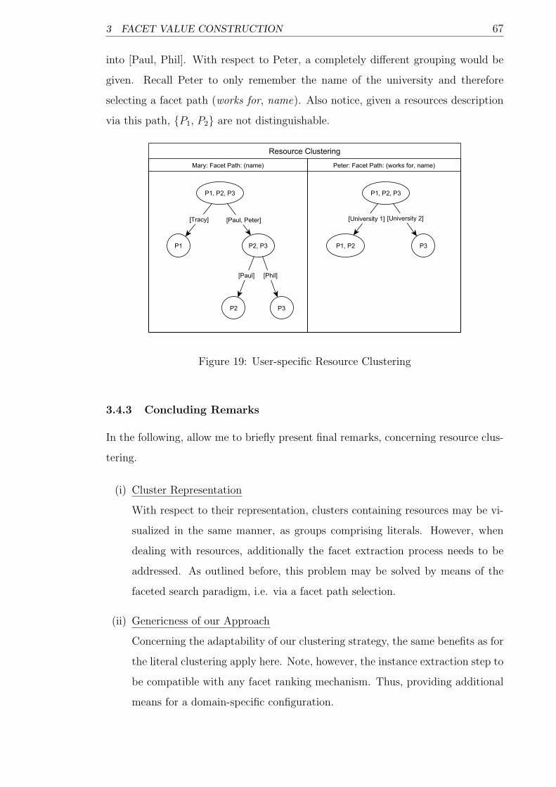
3 FACET VALUE CONSTRUCTION 67
into [Paul, Phil]. With respect to Peter, a completely different grouping would be
given. Recall Peter to only remember the name of the university and therefore
selecting a facet path (works for, name). Also notice, given a resources description
via this path, {P1, P2} are not distinguishable.
Figure 19: User-specific Resource Clustering
3.4.3 Concluding Remarks
In the following, allow me to briefly present final remarks, concerning resource clus-
tering.
(i) Cluster Representation
With respect to their representation, clusters containing resources may be vi-
sualized in the same manner, as groups comprising literals. However, when
dealing with resources, additionally the facet extraction process needs to be
addressed. As outlined before, this problem may be solved by means of the
faceted search paradigm, i.e. via a facet path selection.
(ii) Genericness of our Approach
Concerning the adaptability of our clustering strategy, the same benefits as for
the literal clustering apply here. Note, however, the instance extraction step to
be compatible with any facet ranking mechanism. Thus, providing additional
means for a domain-specific configuration.

3 FACET VALUE CONSTRUCTION 68
(iii) Satisfying above given Clustering Intuitions
Lastly, I would like to outline, how the presented strategy meets our overall
clustering intuitions.
- Traditional clustering Goals
Since I reduced the initial resource clustering problem to a facet ranking
and attribute clustering task, the same arguments as discussed above do
apply here.
- Support of fuzzy knowledge
Again, as a top-down clustering approach is supported, users may articu-
late their information needs in a quite fuzzy or, via drilling down, in very
specific manner.
- Support of partial knowledge
With respect to clustering resources, notice this aspect to target at a
key point. Consider that by giving users full control over the instance
extraction process, they are able to specify their knowledge precisely. By
means of a user-selected facet path, a basis for a similarity measure as
well as a clustering process may be provided, while supporting partial
user information completely.
3.5 Cluster Tree
It is very important for the reader to realize that the structure established by the
described clustering strategies is tree-shaped, thus leading to a notion of a so called
cluster tree. More precisely, flat, as well as non-flat values, are in their nature
hierarchical. Therefore, given a facet f , the partitioning of its values results in a
cluster tree, say Tree(f). Each node n in Tree(f) corresponds to a facet value,
with V (n) denoting literals or resources contained in this cluster. Furthermore, the
current result set is split into subsets, so that each node n may be mapped to a
result cluster. Let R(n) denote the set of all result items being associated with
a value contained in V (n). Note that these sets could be overlapping, as a result
item may have values contained in several different clusters V (n). Thus, in other
words, there are two relations, say V and R, mapping each node n in Tree(f) to
sets V (n) and R(n), respectively. Formally, given a facet f , V may be defined as

3 FACET VALUE CONSTRUCTION 69
V ∶ Nf ↦ P (O∗(f)), whereas R is given by R ∶ Nf ↦ P (V Res) with Nf being a
set, comprising nodes contained in Tree(f). In conclusion, V (n) may be written
as:
Vf(n) = {v ∈ O∗(f) ∣ l(v) = n} (3.16)
with l(⋅) standing for a function, assigning a class label to a given element. Further-
more, R(n) is defined by:
Rf(n) ={v ∈ V Res ∣∃V ⊆ P (O∗(f)) ∶ {v}FnÐ→ V ∧
∃ v ∈ V ∶ l(v) = n∧
F n = (∗, . . . ,∗, f)}
(3.17)
Notice, V (n) and R(n) are hereafter referred to as value and result segmentation,
respectively. Also, please find a generic example for a Tree(f), together with its
relations V and R, provided in the appendix (see figure 24, p. 105).

Section 4
Facet Ranking
4.1 Introduction
Motivation Please remember the introduced facet (see definition 2.11, p. 29) as
well as facet value (see definition 2.12, p. 31) definition. In particular, observe these
notions to be very fine-grained. Thus, given a large and well-structured data-source,
one might have to deal with an overwhelming facet and facet value set, respectively.
That being said, it is obvious for several reasons that a crucial part of a faceted
search system is facet and facet value ranking. Hereafter, allow me to further elab-
orate the need for a ranking heuristic, given our context.
First of all, users tend to have very rarely complete knowledge of their item of in-
terest. Thus, naturally only a small number of facets may be relevant for them. On
the other hand, from a technical point of view, visualizing all available facets and
facet values respectively, would exceed the capabilities of any graphical interface
and will be confusing for users. Lastly, even if users would have complete knowledge
of their item of interest, facets might differ, with respect to their usefulness for the
fulfillment of a particular task. In this context, please recall the above discussion of
varying needs in section 1.1.1 (p. 1). Notice, in the following, I am going to focus
on higher-level needs, which are often associated with little precise user knowledge.
For the outlined ranking purposes, the current cluster tree is taken into consider-
ation. More precisely, ranking is accomplished by defining metrics over the tree
and aggregating them, using an integrated ranking function. Note, I first explain
the intuitions behind the chosen metrics and afterwards describe a specific scoring
function.
Problem Definition Before going into more details on possible applications for
a ranking mechanism or on the actual ranking paradigm, I will first introduce defi-

4 FACET RANKING 71
nitions for facet and facet value ranking functions:
+ Definition 4.1. Facet and Facet Value Ranking Function
Given a resource space SR with gR, a result space SRes with gResi , a query graph gq
and a set F containing all facets, a facet ranking function, say rf , is defined as rf ∶FR ↦ R. In a similar manner, given a facet value fv with fv ∈ FV∗(⋅) ⊆ P (O∗(⋅)),a ranking function, say rv, may be defined as rv ∶ FV R ↦ R.
In simple terms, a ranking function r∗ maps a facet or facet value to a score in R, rep-
resenting its importance, in compliance with application-specific settings and goals.
Given this notion of a ranking function, please find hereafter a formal definition of
the ranking problem, which I will address within this section.
1 Problem 4.1. Ranking Problem
Given a facet f ∈ F , the problem consists of defining a function, which maps a facet
to a ranking score, in compliance with the browsing paradigm as well as a current
result space.
Note, for a facet value, say fv, a problem may be defined in a similar manner.
Use-Cases for Ranking According to my knowledge, there are two common
applications of facet ranking. First, there is the simple sorting of facets or facet
values, in compliance with their ranking weight. Meaning, the higher a weight, the
higher sorted a facet or facet value is, with regard to a list presented to users. The
second common ranking application is a facet hiding strategy. Here, in order to
make the navigation easier and more intuitive for users, less important, i.e. facets
or facet values with low scores associated, are omitted. Users may be provided an
option like show other or show all, for having access to all available facets.
4.2 A short Survey of present Ranking Approaches
4.2.1 Overview
In the following, I would like to provide a short overview of present facet ranking
approaches and their associated paradigms. As mentioned earlier, faceted search
became popular during recent years, thus, also ranking heuristics were discussed ex-
tensively within the research community. However, before looking at more complex

4 FACET RANKING 72
techniques, let us start with a quite easy and straight-forward approach, namely the
so called count-based or frequency-based ranking.
4.2.2 Ranking Approach: Frequency-based Ranking
Frequency-based23 or often also called count-based ranking, is probably the most
commonly used metric. The overall idea is as follows: the more items, contained in
a result space, are associated with a particular facet value pair, the more important
and representative this pair has to be. In compliance with [DIW05], this technique
has the benefit of presenting those facets first that contain the most information.
Thereby, such approaches guarantee lower ranked properties, to comprise only a
small fraction of the result to represent (cf. [DIW05]). For details, please see
[DIW05, KZL08, ODM+06].
4.2.3 Ranking Approach: Set-cover Ranking
Furthermore, according to [DIW05], there is also the so called set-cover -based rank-
ing. “The objective of set-cover ranking is to maximize the number of distinct
objects that are accessible from the top-k ranked categories.”, cf. [DIW05].24 Thus,
their objective is to maximize a function, say Cover, defined as:
Cover(C) = o(C1) ∪ . . . ∪ o(Ck) (4.1)
with C standing for the set of all categories, {C1, . . . ,Ck} being the top-k ranked
categories and o(Cj) referring a function, returning all objects subsumed under a
given category Cj (cf. [DIW05]). [DIW05] apply a greedy strategy for finding a
subset, say C, of C maximizing equation 4.1 (p. 72). The algorithm may be briefly
outlined as follows:
4.2.4 Ranking Approach: Merit-based Ranking
[DIW05] also introduced a ranking technique, targeting at costs associated with
discovering an item of interest. According to their work, user costs may be repre-
sented by the time necessary for the fulfillment of a given information need. More
specifically, given a category C, costs, say T (C), comprise components as follows:
23 Terminology is used in compliance with [DIW05].
24 Note, what [DIW05] refer to as category, I introduced as facet.

4 FACET RANKING 73
Algorithm 1 Greedy set-cover Algorithm
Require: set state of all objects as uncovered
1: repeat
2: Cmax ← C’ having max. number of uncovered objects
3: for all c ∈ Cmax do
4: mark c as covered
5: end for
6: until all objects o ∈ C are covered or ranked k categories
(i) Reading the category headings
In compliance with [DIW05], time spent for reading category headings is said
to be linear in b(Ci) with b(⋅) referring to a function, mapping a given category
to its number of children.
(ii) Correcting mistakes
Given a category Ci and a likelihood, say Pe, for selecting a wrong subcategory,
an additional effort, i.e. Pe(Ci) ⋅ T (Ci), is needed on average, to correct a
browsing mistake (cf. [DIW05])
(iii) Browsing the correct subtree
Lastly, given a category Ci and assuming users to choose a correct subtree,
(1 − Pe(Ci)) ⋅ T (Ci+1) time is necessary, for reaching an item of interest (cf.
[DIW05]).
Therefore, the total time, say T (Ci), is given by:
T (Ci) = κb(Ci)1 − Pe(Ci)
+ T (Ci+1) (4.2)
with κ as a constant. Based on these thoughts, a metric, say merit(C), may be
defined as:
merit(C) =2 ⋅ 1
T (C) ⋅ o(C)1
T (C) + o(C) = 2 ⋅ o(C)1 + T (C) ⋅ o(C) (4.3)
with o(C) as number of objects, having values associated with C (cf. [DIW05]).
4.2.5 Ranking Approach: Interestingness-based Ranking
[DRM+08] introduced a ranking notion centering around the concept of interest-
ingness. More specifically, this well-known concept, originating from the OLAP

4 FACET RANKING 74
community, is redefined as “[. . . ] how surprising an actual aggregated value is,
given a certain expectation”, cf. [DRM+08]. Before having a closer look at this
approach, however, allow me to first give a brief outline over the terminology and
definitions used hereafter:
- A repository, in our terminology the resource space, is denoted by D.
- Dq stands for the set of documents in D, matching a given query q.
- A facet is written as F , while a facet value is given by f .
Now, given {f1, . . . , fn} as facet values, associated with {F1, . . . , Fn}. Furthermore,
assume CD(f1, . . . , fm) to denote the count of documents with respect to D. Sim-
ilarly, Cq(f1, . . . , fm) stands for the count of documents with regard to Dq. Given
E(⋅) as the expected value, in compliance with [DRM+08], the above mentioned
expectations may be computed as described hereafter:
(i) Natural Way
Assume documents, contained in D, are distributed over each facet according
to a natural distribution, e.g. an equal distribution. Also, say all facets are
pairwise independent. Then, according to [DRM+08], for a facet value pair
(F:f), E(Cq(f)) may be given by:
E(Cq(f)) = ∣Dq ∣number of unique values in F inDq
(4.4)
Given (F1,. . . ,Fm:f1,. . . ,fm), on the other hand, we have:
E(Cq(f1, . . . , fm)) = ∣Dq ∣m
∏i=1
Cq(fi)∣Dq ∣
(4.5)
(ii) Navigational
With regard to the so called navigational method, an expectation value is
estimated in accordance with the user navigation. Assume a user issues a
query q1, then counts are set proportionally based on the data distribution in
the repository. In conclusion, E(⋅) is defined as:
E(Cq1(f1, . . . , fm)) = ∣Dq1∣CD(f1, . . . , fm)
∣D∣ (4.6)

4 FACET RANKING 75
Given, the same user enters a second query, say q2, the expectation is recom-
puted as:
E(Cq2(f1, . . . , fm)) = ∣Dq2∣Cq1(f1, . . . , fm)
∣Dq1∣(4.7)
See also [DRM+08].
(iii) Ad hoc
If both methods don’t prove to be suitable, users may set counts for each facet
value proportionally, based on the distribution of a result space, with respect
to an arbitrary query, say q (cf. [DRM+08]).
Making use of the above defined expectation values, [DRM+08] compute their actual
scores as follows. First, they define interestingness for a facet instance. During a
second step, [DRM+08] apply this intermediate result, in order to measure the weight
of an entire facet, say F .
(i) Single facet instance
With regard to a single facet instance, an interestingness score is based on
the actual and expected count. More precisely, say f occurs in r out of R
documents as well as in q out of Q documents, contained in the result set for a
given query. Furthermore, let equation rR > q
Q hold. Given both assumptions,
an interestingness value may be defined as the probability, say p, that a random
set with size Q, contains at least q documents having a facet value f associated.
In accordance with [DRM+08], p is computed as:
q
∑k =0
(rk)(R−rQ−k)
(RQ)
(4.8)
Note, if given rR < q
Q , an interestingness score may be calculated analogously
(cf. [DRM+08]).
(ii) Entire Facet F
In compliance with [DRM+08], one may either use all facet values or just k top-
ranked instances, in order to estimate the interestingness value with regard to
F . Notice, hereafter, I will use the latter option. Thus, given a facet F , one
may consider {f1,...,fk} with p1 < ... < pk. Furthermore, a function Si with
4 FACET RANKING 76
Si = − log(pi) is being computed for each i = 1, . . . , k. Note that S1 ≥ ⋅ ⋅ ⋅ ≥ Skholds. Finally, the degree of interestingness for F is ∑ki=1Wi ⋅ Si with Wi as a
weight (cf. [DRM+08]).
4.2.6 Ranking Approach: Indistinguishability-based Ranking
[BRWD+08] rank facets with regard to their suspected associated navigational costs.
More specifically, they aim at minimizing the necessary users costs, in order to fulfill
an information need. [BRWD+08] argue that facet ranking is very similar to building
a decision tree. “Essentially, the task is to build a decision tree which distinguishes
each tuple by testing attribute values (asking questions). Each node of the tree
represents an attribute, and each edge leading out of the node is labeled with a
value from the attribute’s domain.”, cf. [BRWD+08]. Having such a perspective on
ranking, costs may simply be defined as the expected number of necessary queries,
before reaching an item of interest. Meaning, given a tree, say T , cost(T ) may be
represented by the average tree height, i.e. ∑i h(ti)n with function h mapping leaf ti
to its height (cf. [BRWD+08]). [BRWD+08] use a greedy algorithm for solving this
problem. Hereafter, let me briefly describe it as:
- Use as a root an attribute, say Al, that distinguishes a maximum number of
tuple pairs. Please note, by choosing Al, one divides the data-source, say D,
into subsets Dx1,Dx2, . . . ,Dx∣Doml∣ (cf. [BRWD+08]).
- [BRWD+08] employ the above step, until no further splitting of Dxq is possible.
Formally, [BRWD+08] thereby intend to minimize a so called Indg function, defined
as:
Indg(Al,D) = ∑1≤q≤∣Doml∣
∣Dxq ∣∣Dxq ∣ − 1
2(4.9)
4.2.7 Ranking Approach: Probability-based Ranking
In [KZL08], another ranking technique is presented. In their work, the authors
argue that facet value pairs and thus facets, may be sorted with respect to their
likelihood of being associated with a relevant document.25 Furthermore, [KZL08]
25 Note, in our Semantic Web environment, documents may be seen as resources.

4 FACET RANKING 77
outline two ways for estimating such relevance scores, leading to a personalized
relevance probability as well as a collaborative relevance probability:
(i) Personalized Probability
In the former case, only relevance judgments issued by a particular user are
considered. To be more precise, [KZL08] introduce a framework, which I would
like to outline shortly in the following. Say P (rel ∣u) denotes the likelihood
of a document, contained in the repository, being relevant for a user, say u.
Furthermore, let P (xk ∣ rel, u) and P (xk ∣non−rel, u) respectively be the distri-
bution of facet value pairs xk, given a user u and a relevant and non-relevant
document respectively. Following these thoughts, [KZL08] describe u in a
triple-based manner:
Θu = {P (rel∣u), P (xk ∣ rel, u), P (xk ∣non, u)} (4.10)
(ii) Collaborative Probability
Given the latter case, [KZL08] not only compute relevance scores on the basis
of a single, but of several users. However, gathering that much data from
different sources may easily get expensive. On the other hand, one may assume
that several users share common criteria, interaction patterns or preferences.
Therefore, in accordance with [KZL08], information may be exchanged in-
between users. More precisely, [KZL08] motivate in their work the use of a
Bayesian modeling approach.
4.2.8 Ranking Approach: Mutual Information-based Ranking
In compliance with [KZL08], the well-known mutual information quantity may also
be used for ranking purposes. However, before going into more detail, allow me first,
to shortly remind the reader, how mutual information may be defined (cf. [Sha48]).
Given two discrete random variables, say X and Y , the mutual information between
X and Y , is given by a function I with:
I(X, Y ) = ∑x, y
PXY (x, y) logPXY (x, y)
PX(x) ⋅ PY (y)(4.11)
Please see [Sha48, CT91] for further information. With regard to our ranking con-
text, [KZL08] apply this measure for two random variables, say X1 and X2. Let the

4 FACET RANKING 78
first variable describe the likelihood of a facet value pair being associated with a
document, while the latter one represents the probability of a document being rele-
vant, given a user query. According to [KZL08], those facet value pairs, resulting in
a maximal mutual information score, should be sorted the highest.
4.2.9 Ranking Approach: Descriptors and Navigators
Last, [ODD06] argue that there are two main aspects to be considered, when judging
facets or, to be more precise, their underlying properties: First, facets ranked high,
should describe a dataset and result set respectively. Secondly, facets should enable
users to navigate a data-source (cf. [ODD06]). Hereafter, allow me to outline metrics
the authors developed, aiming at maximizing both criteria.
Descriptors [ODD06] base their argumentation on [Ran62], when reciting that
intuitive facets and properties respectively should be either temporal, spatial, per-
sonal or energetic. Continuing this thought, the authors point out that facets could
be assigned weights, with respect to whether or not they are based on properties
belonging to one of these categories. The necessary meta-data could be provided
by additional ontologies. However, [ODD06] argue that in many use cases such
extensive knowledge is not available, which in turn makes this criterion hard to
employ.
Navigators As described above, [ODD06] regard efficient navigation as a second
key quality criterion. Please note, like [BRWD+08], the authors reduce the ranking
problem to a construction of a decision tree. Thus, hereafter, when referred to a tree,
also a decision tree is meant, which in turn implies a facet sorting. For measuring
how well a given facet supports navigation, [ODD06] propose a metric, comprising
three parts, namely predicate balance, object cardinality and predicate frequency.
(i) Predicate Balance
[ODD06] think of a tree being well-balanced as an important factor for efficient
navigation. The balance of a predicate p, in compliance with [ODD06], is calcu-
lated as:
balance(p) = 1 − ∑ni=1 ns(oi) − µ(n − 1)µ + (Ns − µ)
(4.12)

4 FACET RANKING 79
where ns(oi) represents a distribution of subjects over objects, µ being the mean
vector, Ns the total number of subjects and n standing for the number of possible
objects associated with p.
(i) Object cardinality
A predicate, having a large amount of objects associated, might be confusing
for users and may be difficult to visualize properly, [ODD06] continue. Thus,
the authors argue that an ideal predicate should only have a limited number of
objects. A metric, denoted by card, is estimated as:
card(p) =⎧⎪⎪⎪⎨⎪⎪⎪⎩
0 ifno(p) ≤ 1
exp−(no(p)−µ)
2
2⋅σ2 otherwise(4.13)
(i) Predicate frequency
Lastly, frequency of a given predicate is considered as being important for ef-
fective navigation (cf. [ODD06]). In their work, [ODD06] state that a useful
predicate, say p, should occur frequently within a given data-source, thereby
properly dividing the underlying space. In accordance with [ODD06], the fre-
quency of p, may be defined by means of a function freq as:
freq(q) = ns(p)ns
(4.14)
where function ns(p) returns the number of subjects contained in a data-space
SR, having p as relation associated, and ns referring to the number of distinct
subjects in SR.
4.2.10 Contribution
Please recall our basic assumptions introduced earlier. In particular, remember
assumption 2.3 (p. 21). To be more specific, given users having an information need,
I assume needs contained in QSNeed to be issued via query searching, while unspecific
and fuzzy information, i.e. QFNeed, may be articulated using browsing strategies.
Following these thoughts, one may conclude that facet operations, since representing
basic browsing techniques, will mainly be used for articulation of unspecific and fuzzy
knowledge.
However, reconsidering the above presented approaches, I argue that none addresses

4 FACET RANKING 80
these assumptions properly and enables users to act accordingly. Throughout the
literature, users are expected to be following a specific need as well as having precise
knowledge about their item of interest and the underlying domain. Note, hereafter,
such heuristics are referred to as search-ability-based ranking. In contrast, I aim
at a ranking maxim, preferring those facets and properties respectively that allow
users to issue fuzzy informations needs via browsing techniques. By doing so, I
wish to enable a more exploratory search and thereby the fulfillment of higher-level
information needs (see also section 1, p. 1). Below, I address these shortcomings by
introducing a novel ranking paradigm, namely what I coined browse-ability-based
ranking.
4.3 Facet Ranking with respect to Browse-Ability
4.3.1 Introduction to browse-ability-based Ranking
Basic Assumptions Given above outlined thoughts, in order for a ranking maxim
to result in a meaningful sorting of facets, an approach should rather target brows-
ing, than searching. More precisely, given a setting, as outlined in assumption 2.3
(p. 21), I wish to prefer such facets, which enable users to issue fuzzy information
needs and slowly explore an unknown domain of interest. In other words, facets
should support browsing strategies, given needs solely contained in QFNeed.
Recall, in section 2 (p. 17) I introduced the faceted search paradigm, given a Se-
mantic Web context. With a facet, say f , being based on a property contained
in a resource space SR, there are essentially two interesting sets associated with f ,
i.e. R(n) and V (n). In this context, it is important for the reader to remember
the so called cluster tree, I defined in section 3.5 (p. 68). Given such a facet value
hierarchy as well as relations R and V , projecting nodes to their associated result
item and object sets respectively, one may define metrics, addressing our notion of
browse-ability.
Intuition behind our browse-ability Maxim Hereafter, for clarification pur-
poses, allow me to present intuitions, I believe to be important, with regard to a
browse-ability--based ranking heuristic. More precisely, given a fuzzy information
need, I argue that there are three relevant issues, namely uniform steps to an item
of interest, many steps leading to a single item and a comprehensible result parti-

4 FACET RANKING 81
tioning. Please find these points further discussed below:
(i) Uniform Steps to an Item of Interest
Since I assume needs to be contained in QFNeed, I except users to articulate
rather fuzzy knowledge via means of browsing. For enabling exploration of a
given resource space, I believe that users should be guided in uniform steps
to their item of interest. In particular, with regard to users facing unknown
datasets and having only vaguely information concerning their needs, I argue
that all result items are a priori of equal importance. Thus, it is not possible
to prefer one set of results over another. With respect to a cluster tree, which
users explore, notice that one may not favor a particular path over the others.
(ii) Many Steps leading to a single Item
Related to my first intuition, I further argue that users should be guided in
small steps. More specifically, each exploration step should lead to uniform
and small changes of a given result space. Note, with small steps, I refer to
minor restrictions of a current result set, generated by browsing decisions. I
thereby allow users to slowly dive into an unfamiliar space, rather than rapidly
restrict it to only few specific items. In other words, I wish to avoid rapid drill
downs, which, given our context, are likely to result in browsing mistakes.
The reader should observe this intuition to differ significantly from above im-
plied ones. Reconsider approaches presented in section 4.2.4 (p. 72) or 4.2.6 (p.
76) as examples. Both works intend to minimize user effort needed, for fulfill-
ing a given information task. However, by doing so, the authors rank the most
discriminative facets the highest and thus prefer rapid result set restrictions,
over slow and small ones.
(iii) Comprehensible Result Partitioning
Continuing the above argumentation, I wish to support users in making in-
tuitive decisions at each step, while requiring the least amount of knowledge
possible. Thus, given a cluster tree, users should be able to choose a value,
i.e. a path, without much effort, especially without issuing additional queries.
Note, I refer to a decision as being intuitive, if leading to clear and comprehen-
sible modifications of a result set. More precisely, each decision should lead to
a true restriction, with regard to the current space. Also, given a facet, differ-

4 FACET RANKING 82
ent paths in its associated cluster tree, should lead to different modifications,
i.e. varying sets of result tuples.
4.3.2 Browse-ability-based Ranking: A novel Facet Ranking Approach
4.3.2.1 Indicators for a browse-able Facet
Hereafter, please find specific indicators for the presented intuitions. The reader
should be aware that I first discuss effects on the value segmentation, i.e. V (n), and
afterwards examine the browse-ability notion, with regard to the result space, i.e.
R(n).
Indicators for a browse-able Value Segmentation
(i) Uniform Steps to Item of Interest
Recall, according to the first presented intuition, facets should guide users in
very small, equal-sized steps to their item of interest. Therefore, I believe the
following two indicators might prove useful:
- Height Balance
Since I wish every path, originating from the root and leading to an
arbitrary leaf, to be approximately equal-sized, the tree height might be
of interest. To be more specific, the cluster tree should be height-balanced.
- Equal-sized Value Clusters
Value clusters V (n), with regard to a given hierarchical level in a cluster
tree, should be approximately equal-sized. Meaning, at each hierarchical
level, cluster sizes, i.e. ∣V (n)∣, should only differ by a factor smaller than
a given threshold, say t.
(ii) Many Steps leading to a single Item
Secondly, I argue that users should be guided in small steps to their item of
interest, thereby avoiding rapid space modifications. Below find two indicators
for this intuition.
- Maximal Height
Please remember, I assume users to have no specific knowledge. Therefore,
a rather long path, requiring not much information and leading users to
their item of interest, is desirable.

4 FACET RANKING 83
- Limited Branching Factor
On the other hand, I argue that each hierarchical level should have a
limited number of outgoing branches. Thereby, situations may be avoided,
where users have to choose from a large number of value partitions, i.e.
paths in a cluster tree, which in turn would require specific knowledge.
Indicators for a browse-able Result Segmentation Before looking at more
indicators for measuring the degree of browse-ability, let me motivate how it is
possible that a result clustering is not suitable for browsing, while a browse-able
value space segmentation is given.
. Example 4.1. Hereafter, please see figure 20 (p. 84), as a generic example for
a browse-able value segmentation, leading to a result clustering not being suitable
for browsing. More specifically, while the value clustering clearly fulfills the above
stated indicators, its associated result segmentation leads to rapid drill downs and
thus seems not desirable for slow exploration of an underlying space. Note the
current result set to be circled in green and types, by which resources are grouped,
colored in gray.
In the following, let me introduce influencing factors, I believe to be meaningful
indicators for a result segmentation being regarded as browse-able.
(i) Uniform Steps to Item of Interest
Reconsidering the above mentioned first intuition, i.e. facets should guide users
in uniform steps to their item of interest, I believe the result segmentation size
to be an interesting value. Thus, result clusters, i.e. R(n), associated with
nodes in a cluster tree should be of equal size, so that exploration steps are
uniform, in terms of their effects on a result set. To be more precise, given
a tree level, I compute the maximum cluster size as well as the minimum.
The difference between both values, I then wish to be smaller than a given
threshold.
(ii) Comprehensible Result Partitioning
Remember, I intend a heuristic to support users in making intuitive decisions.
Thus, comprehensible result space interactions are necessary. Below, please
see two indicators, I find meaningful:

4 FACET RANKING 84
(a) Resource Space
(b) V (n) and R(n) for a facet name.
Figure 20: Browse-able V (n) and non-browse-able R(n) Segmentation
- Minimum Result Partition Overlap
Given paths in a cluster tree, I argue that a suitable facet should lead
to a minimal overlap between its associated result segmentations R(n),thereby resulting in different modifications, depending on a user-specific
selection.
- Result Tuple distinguishability
Also, targeting at this intuition, I believe leaves of Tree(⋅) to be an inter-
esting pointer. More precisely, distinguishability is defined with regard to
R(n) segments at leaf level, i.e. one may simply compare the cardinality
of these sets, with a desired threshold value.

4 FACET RANKING 85
4.3.2.2 A Metric for Browse-ability
In the following, I will propose a metric applying the presented indicators and
thereby realizing our browse-ability intuitions. Note, I distinguish between facets
that are based on attributes and those based on relations.
Attribute-based Facets Hereafter, I define metrics for attribute-based facets,
measuring their individual indicators and aggregating them, resulting in a final
score. Furthermore, I will distinguish between metrics measuring effects on the
value space, i.e. V (n), and other metrics applying to the result set segmentation,
i.e. R(n). Given an attribute-based facet f , its cluster tree Tree(f), N as a set,
containing its nodes as well as r referring to its root, measures are as follows:
(i) Measures for a browse-able Value Segmentation
(a) Maximal Height26
A height function h, i.e. h ∶ N ↦ N0, with regard to a given node, say n,
may be defined as the maximal distance from n to a leaf. Furthermore, in
a top-down manner, a height score is calculated as: Given an inner node
n, with nk = ∑i ∣subtreei(n)∣ as its associated size, its deviation from the
maximal possible height is: ρVh = h(n)nk
∈ [0,1]. However, the higher a node
is located, with respect to a given root, the more important fluctuations
are. Thus, I suggest a weight function, depending on h(n), to be applied.
Notice, this weight is only required to be a strictly monotonically decreas-
ing function, e.g. ω(n) = clog(∣n∣+ε) ∈ [0,1] with k ≥ 1 and c as constant. In
conclusion, a height score may be given by:
scoreVρh(n) = ω(n)ρVh (n) ∈ [0,1] (4.15)
(b) Cluster Tree should be height-balanced
Furthermore, I compute in a top-down manner a height balance score as
follows: Given an inner node n with k subtrees {sj}j, each having a height
hj, the maximum height difference is: δVh (n) = 1 − maxt{ht}−mint{ht}h(n) ∈ [0,1].
A height balance score for node n, thus, may be written as:
26 Note the node height to be approximated in my implementation.

4 FACET RANKING 86
scoreVδh(n) = ω(n)δVh (n) ∈ [0,1] (4.16)
(c) Value Clusters V (n) should be equal-sized
Concerning the size balance, a score is computed in the following manner:
Given an inner node n having k subtrees {sj}j associated, size differences
may be estimated by: δVs (n) = 1 − maxj{V (sj)}−minj{V (sj)}V (n) ∈ [0,1]. Again, I
argue that the higher n is located in a tree, the more important fluctuations
are. Therefore, a final score for n is given by:
scoreVδs(n) = ω(n)δVs (n) ∈ [0,1] (4.17)
(d) Limited Branching Factor of Tree(f)Lastly, given an inner node n as well as a function e, mapping n to its
outgoing edges, a deviation from a branching threshold, say κ, is: ρVe (n) =∣κ− e(n)∣e(n) ∈ [0,1]. Following the above thoughts, an edge deviation score is
computed as:
scoreVρe(n) = ω(n)ρVe (n) ∈ [0,1] (4.18)
(ii) Measures for a browse-able Result Set Segmentation
(a) Value Clusters R(n) should be equal-sized
A score, with regard to result cluster size deviations, may be computed
similarly to the above defined scoreVδs , as:
scoreRδs(n) = ω(n)δRs (n) ∈ [0,1] (4.19)
where δRs denotes the size deviation.
(b) Result Tuple distinguishability27
Concerning the distinguishability of tuples contained in a result space, a
score may be calculated as: Given a node n, consider only its leaves, say
{l1, . . . , lm}. Also, let L, i.e. L ∶ N ↦ L and L ⊆ P (N), be a function
mapping each node in N , to a set containing its reachable leaves. Fur-
thermore, λR(n) = ∑l ∈L(n) ∣R(l)∣−1
∑l ∈L(n) ∣R(l)∣∈ [0,1] may be used to estimate the
27 Note, due to performance reasons this score is approximated in my implementation.

4 FACET RANKING 87
distinguishability with regard to n. Again, I will use ω as defined above.
In conclusion, a distinguishability-based score for node n is given by:
scoreRλ (n) = ω(n)λR(n) ∈ [0,1] (4.20)
(c) Minimum Result Segment Overlap
Lastly, I compute a score, measuring the overlap between a given pair of
result segmentations as: Given a node n, let C, i.e. C ∶ N ↦ C and
C ⊆ P (N), denote a function mapping each node in N to its directly
associated children. Therefore, the overlap may be represented as ϕR(n) =1 − ∣⋂ci∈C(n)R(ci)∣
∣R(n)∣ ∈ [0,1]. Furthermore, a score is given by:
scoreRϕ(n) = ω(n)ϕR(n) ∈ [0,1] (4.21)
(iii) Final Score
Let F ′ ∶ R ↦ [0,1] denote a strictly monotonic increasing function. Then,
aggregating the before measured indicators, a final score for an attribute-based
facet is defined as:
scorea(f) = F ′(scoreVδh(r), . . . , scoreRϕ(r)) ∈ [0,1] (4.22)
Relation-based Facets In the paragraph above, I introduced a ranking metric
for attribute-based facets. Hereafter, I intend to expand this definition, to also
include facets based on relations. The ranking score of a relation-based facet, say
f , with facet values FV (f) associated, consists of two parts:
(i) Score, with respect to attributes connected to FV (f). Each attribute score
incorporates elements as follows:
- Browse-ability of V (n).
- Browse-ability of associated result set segmentation R(n).
(ii) Score, with respect to nearby browse-able entities, comprised by a set, say
FV ′(f). In this latter case, one has as influencing factors:
- Distance from FV (f) to FV ′(f).
- Browse-ability of V ′(n).
- Browse-ability of associated result set segmentation R′(n).

4 FACET RANKING 88
Obviously, in order to avoid cycles and guarantee an algorithm to terminate, a
distance threshold is necessary. First of all, however, find below both presented
factors, outlined in more detail.
(i) Score with respect to Attributes
Given a set of m attributes, say A = {fa1 , . . . , fam}, associated with resources
contained in FV (f), one may compute a score as described earlier for each
facet contained in A. This results in SA = {scorea(fa1 ), . . . , scorea(fam)}, i.e.
a set of scores, which may be aggregated via F ′′, resulting in:
scorear(f) = F ′′(scorea(fa1 ), . . . , scorea(fam)) ∈ [0,1] (4.23)
with F ′′ being a strictly monotonic increasing function. Please note, hereafter,
I will refer to this score as attribute-based score.
(ii) Score with respect to nearby browse-able Entities
Recall, resources in FV (f) may be connected via relations to further indi-
viduals, which in turn may or may not be suitable for browsing. Thus, I
argue that one also needs to rank FV (f), with respect to the browse-ability
of its nearby entities. In conclusion, given a set of n relation-based facets, say
R = {f r1 , . . . , f rn}, associated with FV (f), a score may be recursively defined
in a similar manner as introduced earlier.
(iii) Final Score
Lastly, with respect to its relations as well as its attributes, f may be assigned
a total score given by:
scorer(f, k) =⎧⎪⎪⎪⎪⎨⎪⎪⎪⎪⎩
δ(k) scorear(f) if k = kmax
∑f ′∈R F ′′′(scorer(f ′, k + 1), δ(k + 1) scorear(f ′)) otherwise
(4.24)
with k as current hop-distance, kmax as maximum hop threshold, δ being a
monotonic decreasing weight function and F ′′′ as a strictly monotonic increas-
ing function.
For clarification purposes, please see a toy example provided below.

4 FACET RANKING 89
. Example 4.2. After exploring the profile of Frances E. Allen, Mary continues
her search for famous scientists. Unfortunately, she can’t recall any further names,
Peter mentioned the other day. Therefore, in her case, a discriminatory facet such as
name, having e.g. values {Jane,Rachel, Peter}, should not be ranked high. More
specifically, given such a value set, name is a unique identifier, thus leading to rapid
result set modifications. In particular, name forces Mary to instantly decide what
entity to choose, which in turn requires very specific knowledge. Plus, it does not
provide the necessary freedom to properly explore the given result set. On the other
hand, a facet such as type or works at, might prove more suitable. E.g. via works
at, a cluster tree of greater height may be constructed. Thereby allowing Mary to
iteratively chose a path along this tree, while exploring the space. On the other
hand, type would result in smaller modifications of the current result, as several
scientists may share a common value, e.g. PhD-Student. Thus, by means of type,
Mary is able to slowly and iteratively familiarize herself with this unknown domain.
Concluding Remarks Below, please find concluding remarks, targeting at fur-
ther aspects of our browse-ability-based ranking approach.
(i) Choosing a proper Aggregation Function
Note, the above defined aggregation functions, i.e. F ∗, are only required to be
strictly monotonic increasing. Obviously, there are several meaningful ways to
implement F ∗, consider e.g. F ∗ (⋅) = max{⋅}, F ∗ = min{⋅} or F ∗(⋅) = avg{⋅}.
Furthermore, as different functions have varying impacts on a browse-ability
score, it might be wise to use an application-specific realization. However, in
order to keep the metric as generic as possible, I left F ∗ defined in a fuzzy man-
ner. Note, I currently implemented these aggregation functions as weighted
summations.
(ii) Choosing a proper Weight & Discount Function
For the same reason, namely to define our browse-ability metric in a generic
manner, I also left ω as well as the discount function δ open, to be implemented
later on. Note, due to performance reasons, I realized the weight function
simply as ω(n) = ∣R(n)∣∣Rtotal∣ with Rtotal = ∣V Res∣. Furthermore, since I used a strict
distance threshold kmax = 1, there was no need for a discount mechanism δ.

4 FACET RANKING 90
(iii) Integration of Property Hierarchies
Recall, a subproperty-of link between two given properties, say p1 and p2,
indicates a subset relation, with respect to their domain as well as their range.
Thus, given p1 and p2, their associated ranking scores are obviously correlated.
However, as a simple workaround for this dilemma, I group properties and
facets respectively, so that there is no subproperty-of connection between any
facet pair, presented to users at the same level. Note, by grouping I mean a
clustering strategy, making use of property hierarchies.
(iv) Facet Value Ranking
Lastly, the facet ranking strategy, as discussed above, is based on ranking
nodes in a cluster tree. Thus, transferring the introduced indicators and mea-
surements, to also cover facet values contained in FV∗(⋅), is fairly easy. Given
an attribute-based facet, say f , and a facet value, say v, e.g. scorea might be
rewritten as:
scorea(v) = F ′(scoreVδh(nv), . . . , scoreRϕ(nv)) ∈ [0,1] (4.25)
with nv being the node in N , associated with v.

Section 5
Evaluation
5.1 Evaluation Setting
Since the overall intuition behind our faceted search application is, to enable a more
effective way of browsing in an unknown resource space, I felt that a user-oriented
evaluation with focus on fuzzily defined tasks would be best. Thus, for assessment
of the novel ranking scheme, as well as the discussed facet value clustering approach,
I chose a task-based user study.
User Tasks I divided the evaluation process in two steps: The first part covers
the ranking strategy, while the latter one addresses our value clustering. Each part
contained 12 tasks. Correspondingly, I formed two groups of participants. Each is
associated with a set of 12 tasks, resulting in a total of 24 tasks.
With regard to the ranking mechanism, I presented six tasks to each user. In
four of these tasks, a very fuzzy and unspecific information need was given to the
subject, e.g.: Starting with a keyword search for Karlsruhe. Find an entity having
something to do with traveling. For the remaining two tasks, I gave users a very broad
exploration task, i.e. to find outlier, interesting or strange values. Consider as an
example: Start with keyword search Karlsruhe. Explore the given result set. Note,
for a complete list of tasks, please see table 2 (p. 108), provided in the appendix.
Hereafter, the first type is referred to as ranking type (a), while the latter group
of tasks may be denoted by type (b). Evaluation subjects were only allowed to
use the five top-ranked facets during their assignments. Also, for tasks of type (a),
one group was only presented a search-ability-based sorting, while the other one
was given a ranking, based on our browse-ability approach. For assignments (b), on
the other hand, subject groups were given two different sortings, i.e. one for each
ranking scheme.

5 EVALUATION 92
As for the second group of tasks, being concerned with facet value clustering, again
a situation was simulated, where users faced imprecise and fuzzy information needs.
There were two sets comprising six tasks each, therefore assigning twelve tasks in
total. More precisely, in each set, two tasks were targeting literal clustering, while
four other tasks correspond to our resource clustering strategy. To give the reader
an idea of these tasks, please consider the following to two examples: (i) For the first
group, i.e. the literal clustering tasks, one assignment was: Start with keyword search
for London. Find all artists (an artist is a person) born some time in November
1972. Notice, in the following, this set is denoted by type (a). (ii) Concerning the
clustering of resources, please consider as exemplary task: Start with keyword search
for Paris. Find all Things, having as genre a music genre, which has as instrument
an electric guitar. Hereafter, this set of tasks is referred to as type (b). Again, a
complete list of tasks is provided in table 2 (p. 108). Further notice, for solving their
assignments, evaluation subjects first used our system, having a clustering approach
implemented, and afterwards, a baseline system, providing no clustering.
Evaluation Subjects In total, there were 24 subjects taking part in the evalua-
tion. However, the reader should notice, our participants to have very heterogeneous
backgrounds. In particular, six users had no experience with computer science tech-
nologies at all. Furthermore, of the remaining 18 subjects, 10 had no or only very
little experience with Semantic Web technologies. On the other hand, all partici-
pants were familiar with search technologies common in the WWW.
Time-based Interaction Costs With regard to user effort, I argue that refine-
ment, expansion and browsing interactions are crucial for the time needed to fulfill
an information task. In the following, these operations are defined as intervals. To
be more specific, browsing comprises operations, which users perform, in order to
select a facet, navigate along a facet path or drill down into a given cluster tree.
Accordingly, a browsing interaction is defined as a time interval, staring with the
completion of a last browsing operation and terminating, as users move to the next
node in the hierarchy or decide to abort browsing this particular facet. On average,
I measured users to need 4.4 sec for a single interaction. On the other hand, I col-
lected the time users required, to modify a given space. Note, this means adding a
terminal node in a cluster tree, i.e. a facet value node, which restricts results to only

5 EVALUATION 93
those, fulfilling the additional constraint, or removing one respectively. Accordingly,
the time interval spans from the completion of a browsing operation, until users add
such a node (refinement) or remove one (expansion). Here, I measured 8 sec in the
former and 18 sec in latter case, on average.
System With respect to the system employed, I made use of the Information
Workbench, providing means for a collaborate management of data and publicly
accessible at http://iwb.fluidops.com/. The faceted search layer has been realized
using Java Berkeley DB and Lucene, based on design patterns and index structures
introduced in [BYGH+08, DRM+08]. More precisely, while the back-end, including
the keyword and faceted search modules, was implemented in Java 6, the front-end
uses Ajax technologies, running on a Jetty server. Experiments were carried out
in a supervised manner, on a PC with a T7300 Intel CPU, 4 GB memory and a
Microsoft Vista OS. The search process for each user and task was recorded via a
screencast.
Data Concerning the data-source, I used DBpedia, which is covering a large amount
of broad-ranging knowledge [BLK+09]. This enabled me to design evaluation tasks,
not targeted at a specific field, but being rather domain-independent.
5.2 Browse-ability-based Ranking
5.2.1 Baseline for Ranking Evaluation
Search-ability-based Ranking As introduced in section 4.2 (p. 71), much of
the recent work is devoted to search-ability-based ranking. Thus, I decided to com-
pare our approach against this type of schema. However, I did not implement a
particular strategy, but rather intended to use the abstract search-ability paradigm
as a baseline. I developed a heuristic, reflecting this intuition on a higher-level,
written as a monotonic aggregation function M with M(h,λR, ϕR).28 Correspond-
ingly, M targets at reducing users costs, in particular, the amount of interactions
necessary to fulfill an information need. More precisely, the tree height, say h, is
minimized and thereby user decisions required are being reduced. Furthermore,
facets should be discriminative. Thus, I prefer those facets, leading to results with
28 Note that currently M is simply realized as a weighted summation.

5 EVALUATION 94
high distinguishability score as well as few result segment overlaps, given by λR and
ϕR respectively.
5.2.2 Ranking Effectiveness
Regarding effectiveness of search-ability versus browse-ability ranking, I compared
the average success rate of tasks of type (a), as well as the average browsing expe-
rience, for tasks of type (b). Results are provided in figure 21(c) (p. 95) as well as
21(c) (p. 95) to the reader. Here, I observed, given search-ability-based ranking, par-
ticipants succeeded in tasks, where small result sets, i.e. less than 50 items, had to
be explored. To be more specific, on the one hand, users selected facets for browsing
and refinement in a brute-force manner (cf. tasks 1.1, 1.4, 1.5, 1.11). On the other
hand, some participants had specific background knowledge (cf. task 1.2), enabling
them to solve their tasks. However, if a keyword search resulted in larger sets, i.e.
more than 150 hits, I noticed participants not being able to accomplish their tasks
(see tasks 1.7, 1.8, 1.10). Browse-ability ranking outperforms the baseline, with re-
gard to all assignments, particularly, given large sets for exploration. Furthermore,
I noticed participants to prefer non-discriminating or unspecific facets, e.g. type or
genre, over specific ones, e.g. population or name. In many cases, I noted subjects
using type for an initial restriction, followed by further exploration via other facets.
Concerning the second type of assignments, i.e. a exploration a given space, browse-
ability-based ranking also performs very well. Please consider figure 21(c) (p. 95).
Overall, exploration using our novel scheme was rated by participants between 4 and
4.5, given a scale [1–5]. Facets sorted with regard to search-ability ranking, on the
other hand, were regarded as not suitable for exploration purposes. This setting was
rated between 2 and 2.7. I explain this result with users not being able to explore
or understanding a result set, by means of specific and discriminative facets.
5.2.3 Ranking Efficiency
Please see figure 21(a) (p. 95) for the average users costs, measured with regard to
a time effort, users needed to fulfill their tasks. Similar to the effectiveness study, I
observed the number of results to be a crucial factor, with respect to the problem
solving strategies applied: On the one hand, given a small result set (less than 50
hits) to browse as well as a search-ability-based heuristic, participants tend to fulfill

5 EVALUATION 95
their assignments with equal or less effort on average, as compared to our approach
(cf. tasks 1.1, 1.2, 1.4, 1.5). More specifically, users were able to efficiently choose
paths in a provided cluster tree and refine a space, using a goal-oriented manner,
leading to less associated costs. When having larger result sets (more than 150 hits)
provided, on the other hand, more time and effort was necessary or participants were
not able to solve their assignments at all (see tasks 1.11, 1.7, 1.8 or 1.10). Note that
task 1.11 was not completed by all users, however, if fulfilled, subjects made use of
a brute-force-like approach, in order to cover all paths. Therefore, I conclude that
while not necessarily leading the cheapest way to an item of interest, our approach
seems to perform well, given large spaces combined with fuzzy needs.
(a) Average effort (type a) (b) Average exploration (type b)
(c) Average success rate (type a)
Figure 21: Efficiency & Effectiveness Results w.r.t. Ranking Schema

5 EVALUATION 96
5.2.4 Ranking Usability
Lastly, I intended to estimate the general usability of our ranking technique. In
this context, please recall the evaluation subjects to have a fairly heterogeneous
background. After completing their assignments and having worked with both ap-
proaches, each subject was asked how useful the browse-ability-based strategy has
proven itself as well as how intuitive a sorting has been. See also the complete ques-
tionnaire, provided to the reader in table 3 (p. 110). Given a scale [1–5], ratings
were quite good, namely for the former question a 4.31 and for the latter one a 4.17,
on average.
5.3 Facet Value Construction
5.3.1 Baseline for Clustering Evaluation
With respect to the evaluation of the clustering technique, producing a hierarchical
facet value structure, finding a fitting baseline was non-trivial. Note, I’m not aware
of any faceted search system, be it in the commercial or in the academic field, using
clustering as means to partition a facet range. Thus, I decided to use a traditional
approach, i.e. a system employing no clustering for either literals or resources.
However, notice the chosen system to work on a similar data-source, i.e. DBepdia.
Also, it is publicly available at http://dbpedia.neofonie.de.
5.3.2 Clustering Effectiveness
Concerning literal clustering, I observed that, given a specific information need, there
is not much of a difference between our system and the baseline (cf. task 2.7, figure
22(b), p. 98). However, the more fuzzy information needs are, the more I noticed
users to depend on clustering being provided, in order to solve their assignments
(see tasks 2.1, 2.4, 2.10). Please consider task 2.10, where a fuzzy need is given.
Without clustering enabled, I observed some users to be not willing to fulfill this
assignment, because of the extra effort needed, while other subjects seemed not to be
aware of ways to complete it. If clustering was given, on the other hand, participants
achieved overall a high success rate (cf. figure 22(b), p. 98). I explain these results
with our clustering techniques enabling participants to articulate fuzzy needs in a
fairly easy manner. Subjects seemed to handle drill down operations as a mean for

5 EVALUATION 97
slowly specifying knowledge well.
With respect to resource partitioning, users did not manage to complete their tasks
using the baseline system (cf. figure 22(c), p. 98). Again, a number of participants
did notice and outline possibilities of solving their assignments, but also realized the
substantial time required and balked the effort. On the other hand, having means
of value partitioning provided, a success rate of over 67 percent was achieved (cf.
figure 22(c), p. 98). These results are very promising, as all tasks involve high-level
information needs that can only be satisfied by means of complex, more-hop queries.
To be more specific, participants solved assignments via iterative construction of
facet paths. I explain these accomplishments with faceted search being a well-
known and well-accepted paradigm. Many users seemed to very intuitively choose
the correct path.
5.3.3 Clustering Efficiency
Given this context, I again distinguish between clustering of literals and clustering
of resources. In the former case, I observed that, if participants managed to fulfill
their assignments, they made use of a brute-force-like strategy, in order to explore
the entire result space. Obviously, such a strategy is very expensive in terms of user
effort, as it requires more system interaction (cf. tasks 2.1, 2.4, figure 22(b), p. 98).
On the other hand, given tasks involving a specific information need, I noted many
participants to use query searching as a strategy to fulfill their assignment. This
resulted in both strategies having an equal performance, with regard to user effort.
As a matter of fact, our approach tends to be slightly more expensive, as sometimes
more browsing interactions were necessary (cf. task 2.7).
Concerning the latter case, i.e. the clustering of resources, I already outlined above
that during the evaluation no participant succeeded using the baseline system (cf.
figure 22(c), p. 98). However, it is important for the reader to notice that trivial
tasks, requiring only a simple, one-hop restriction of values in FV (e.g. constraining
entities via name), may have been easily completed in both systems. Actually, I
expect that browsing strategies would have led to higher users costs, when compared
with query searching.

5 EVALUATION 98
(a) Average user costs (type a
& b)
(b) Average success rate (type a)
(c) Average success rate (type b)
Figure 22: Efficiency & Effectiveness w.r.t. Clustering
5.3.4 Cluster Usability
Especially in combination with high-level information needs, usability is an impor-
tant issue. Thus, after completing their assignments, users were given a set of
questions, targeting at usability aspects of the clustering technique. For details,
please see table 3 (p. 110). In particular, users were asked to rate how useful and
how intuitive the clustering has been. Note, results achieved were quite good. More
precisely, concerning the former question, users judged the clustering strategy to be
a 4.5 and, with respect to the latter one, a 3.8 (given a scale [1–5]). Asking the same
for resource clustering, users again seemed quite satisfied, rating the usefulness a 4.6
and the intuitiveness a 4.2.

Section 6
Conclusion
Concluding Remarks The web of data nowadays offers a vast amount of in-
formation, allowing complex and high-level user needs. However, in order to issue
such needs, one is required to employ a specific query language as well as to possess
precise knowledge about the underlying domain and an item of interest. Faceted
search, on the other hand, as a newly emerging paradigm, offers ways for users to it-
eratively issue their queries, without having to use a given language. Thus, enabling
users to browse an unfamiliar space, without having prior knowledge of its schema
or syntax. State of the art faceted search approaches, however, focus rather on sup-
porting query searching than browsing strategies. As a result, current systems do
not enable exploration and thus seem not suitable for high-level information needs,
given a certain fuzziness, with regard to user knowledge.
Addressing this weakness, I presented in section 3 (p.36) techniques for clustering
of resources and literals, resulting in more browse-able facet values, which explic-
itly support fuzzy user information needs. Continuing in section 4 (p. 70), a novel
ranking scheme, targeting at support of exploration of an unknown resource space,
was introduced. This browse-ability-based ranking is designed to prefer such facets,
which guide users in small and non-discriminatory steps to their item of interest,
while resulting in observable and comprehensible result set modifications. Lastly,
in section 5 (p. 91), by means of a task-based user study, involving 24 participant
as well as 24 tasks, I evaluated these approaches. The results seem very promising,
as they clearly indicate that these techniques outperform state of the art systems,
given users with vague information needs. On the other hand, I noticed that par-
ticipants having specific knowledge, were able to fulfill their assignments with less
effort using traditional systems, i.e. approaches addressing search-ability. Therefore,
I conclude that while not necessarily leading the cheapest way to an item of interest,

6 CONCLUSION 100
browse-ability-based strategies enable users to explore and search more effectively.
Future Work Concerning our future work, I wish to target a tightly integrated
approach using both paradigms, i.e. search-ability as well as browse-ability. Clearly,
depending on user background knowledge and specificity of an information need, the
former or latter strategy, may be more or less suitable. Furthermore, the runtime
performance was currently not addressed properly, leading to high I/O during a
search phase. Thus, a more efficient index structure, supporting common operations,
like facet browsing, refinement or expansion is needed. The reader should be aware
that state of the art structures29, are not applicable in our context, as they do
not scale well, with regard to our fine-grained facet and facet value definition (see
section 2, p. 17). A novel index design, adressing both, i.e. space complexity and
time complexity, is necessary.
29 Consider e.g. http://lucene.apache.org/solr/, a Lucene-based faceted search system, revised
Dec. 2009.


APPENDIX 102
Appendix
RDF Properties
Name Domain Range
rdf:type rdfs:Resource rdfs:Class
rdfs:isDefinedBy rdfs:Resource rdfs:Resource
rdf:value rdfs:Resource rdfs:Resource
rdfs:label rdfs:Resource rdfs:Literal
rdfs:comment rdfs:Resource rdfs:Literal
rdfs:member rdfs:Resource rdfs:Resource
rdfs:seeAlso rdfs:Resource rdfs:Resource
Table 1: Relevant predefined Properties in RDF(S) language

APPENDIX 103
XML Schema built-in Datatypes
Figure 23: XML Schema built-in Datatypes (based on [BM04])

APPENDIX 104
Pseudocode for Literal Clustering
Algorithm 2 Pseudocode for Literal Clustering
Require: k ←branching factor
Require: L ← {li}1≤ i≤k //L is assigned all literals within this range
1: Q ← ∅ //Initialize sets.
2: C ← ∅
3: L ← ∅
4: L ← sort(L) //L is sorted with respect toL⪯
5: for all li, li+1 ∈ L do
6: dcurrent ← dissimilarity(li, li+1)
7: Q ← Q ∪ {dcurrent}
8: end for
9: Q ← sort(Q) //Q is sorted
10: C ← C ∪ {L} //Begin clustering. Top-level cluster is added first.
11: repeat
12: i ← 1
13: while i ≤ k do
14: dmax ← pop(Q) //Obtain and remove maximum distance from Q.
15: ccurrent ← cluster(dmax) //Get cluster with maximum distance.
16: C ← C / ccurrent
17: (c1, c2) ← split(ccurrent, dmax) //Split ccurrent at position dmax.
18: C ← C ∪ c1 ∪ c2
19: i ← i + 1
20: end while
21: until (Q = ∅) ∨ (no drill-down is performed)

APPENDIX 105
Generic Cluster Tree Example
Figure 24: Generic Cluster Tree Example

APPENDIX 106
Evaluation
Evaluation Tasks
Evaluation of . . . Task No. Task Description
Ranking (A)
1.1 Start with keyword search Karlsruhe.
Find something (prefer top ranked facets),
where people live and doesn’t fit in.
1.2 Start with keyword search Karlsruhe. Ex-
plore (prefer top ranked facets) the given
result set: Find an item that got some-
thing to do with traveling.
1.3 Start with keyword search Karlsruhe. Ex-
plore (using only the top five facets) the
given result set.
1.4 Start with keyword search Heidelberg.
Find something (prefer top ranked facets),
having to do with sports and that doesn’t
fit in.
1.5 Start with keyword search Heidelberg. Ex-
plore (prefer top ranked facets) the given
result set: Find an item that’s got some-
thing to do with music.
1.6 Start with keyword search Heidelberg. Ex-
plore (using only the top five facets) the
given result set.
Clustering (A)
2.1 Start with keyword search for Paris. Find
all places, having names starting with
’Paris, I . . . ’, ’Paris, J . . . ’ or ’Paris,
K . . . ’. Of those places, which one is the
smallest (population wise]?
Table continued on next page . . .

APPENDIX 107
Table 2 - Continued
Evaluation of . . . Task No. Task Description
2.2 Start with keyword search for Paris. Find
all things, having as genre a music genre,
which has as instrument an electric guitar.
2.3 Start with keyword search for Paris. Find
all works, having an actor as writer.
2.4 Start with keyword search for London.
Find all artists (an artist is a person),
born some time in November 1972. Also,
find out in which area(s) those people were
born.
2.5 Start with keyword search for London.
Find all works, having as subsequent work
a television show (episode).
2.6 Start with keyword search for London.
Find all works, having an artist born 1926.
Ranking (B)
1.1 Start with keyword search Barcelona.
Find an educational institution (prefer top
ranked facets) not quite fitting in.
1.2 Start with keyword search Barcelona.
Find an international jazz-band drummer
(prefer top ranked facets), who played to-
gether with Louis Armstrong.
1.3 Start with keyword search Barcelona. Ex-
plore (using only the top five facets) the
given result set.
1.4 Start with keyword search Seattle. Find
a hospital for minors (prefer top ranked
facets).
Table continued on next page . . .

APPENDIX 108
Table 2 - Continued
Evaluation of . . . Task No. Task Description
1.5 Start with keyword search Seattle. Find an
international Airport (prefer top ranked
facets).
1.6 Start with keyword search Seattle. Explore
(using only the top five facets) the given
result set.
Clustering (B)
2.1 Start with keyword search for Berlin. Find
the orchestra ’Berliner Philharmoniker’.
2.2 Start with keyword search for Berlin. Find
a work, having as producer someone who
is also a musical artist.
2.3 Start with keyword search for Berlin. Find
a work, having as artist a band (a band is
an organization), which has their home-
town located in Japan.
2.4 Start with keyword search for Hamburg.
Find all places, having a name starting
with ’K’, ’L’, ’M’, ’N’ or ’U’. Which of the
above places is not located in Germany?
2.5 Start with keyword search for Hamburg.
Find all works, having as artist a solo-
artist. Select the latest of the above works.
2.6 Start with keyword search for Hamburg.
Find some building, owned by an organi-
zation, founded in the early 20th century.
Table 2: User Tasks for Evaluation

APPENDIX 109
Evaluation Questionnaire
No. Question
1Reconsider task 1.1/1.2/1.4/1.5. How helpful was the facet ranking
for completing this task?
p Very Helpful. p Pretty Helpful. p Sometimes Helpful.
p In most cases not helpful. p Not helpful at all.
—
2Reconsider task 1.1/1.2/1.4/1.5. Did you have any previous knowl-
edge about the item of interest?
I had no previous knowledge. Tasks: I had some knowledge.
Tasks: I had full knowledge. Tasks:
—
3Reconsider task 1.3/1.6 . In your opinion, how well did you explore
the given result set (scale [1–5])?
a.) Using the browse-ability ranking: b.) Using the search-
ability ranking:
—
4With respect to exploration as our goal, how intuitive was the
browse-ability-based facet ranking?
p Very intuitive. p Understandable. p Fairly intuitive.
p Sometimes unclear. p Not intuitive at all.
—
5Reconsider task 2.1/2.4. How intuitive was the literal clustering?
p Very intuitive. p Understandable. p Fairly intuitive.
p Sometimes unclear. p Not intuitive at all.
—
6Reconsider task 2.1/2.4. How helpful was the literal clustering for
completing the tasks?
p Very intuitive. p Understandable. p Fairly intuitive.
p Sometimes unclear. p Not intuitive at all.
Table continued on next page . . .

APPENDIX 110
Table 3 - Continued
No. Question
7Reconsider task 2.2/2.3/2.5/2.6. How intuitive was the resource
clustering?
p Very intuitive. p Understandable. p Fairly intuitive.
p Sometimes unclear. p Not intuitive at all.
—
8Reconsider task 2.2/2.3/2.5/2.6. How helpful was the resource clus-
tering for completing the tasks?
p Very intuitive. p Understandable. p Fairly intuitive.
p Sometimes unclear. p Not intuitive at all.
—
9How would you describe the search experience in comparison with
classical information search systems (like Google or Wikipedia)?
p I liked the new features a lot. p The new features were
interesting. p The new features were interesting, but a little
confusing. p The new features made searching harder.
—
10Would you use the system again?
p Yes, definitely. p Maybe. p Not very likely. p No,
definitely not.
—
11Did you have any other problems while using the system? What did
you like? What did you not like?
Comments:
Table 3: Questionnaire for Evaluation

REFERENCES 111
References
[ABC+02] B. Aditya, Gaurav Bhalotia, Soumen Chakrabarti, Arvind Hulgeri,
Charuta Nakhe, Parag Parag, and S. Sudarshan. Banks: browsing
and keyword searching in relational databases. In VLDB ’02: Proceed-
ings of the 28th international conference on Very Large Data Bases,
pages 1083–1086. VLDB Endowment, 2002.
[AvH08] Grigoris Antoniou and Frank van Harmelen. A Semantic Web Primer.
The MIT Press, 2 edition, March 2008.
[Bat02] Marcia J Bates. Speculations on browsing, directed searching, and
linking in relation to the bradford distribution. In Peter Ingwersen
Pertti Vakkari Harry Bruce, Raya Fidel, editor, Emerging Frameworks
and Methods: Proceedings of the Fourth International Conference on
Conceptions of Library and Information Science, pages 137–150, 2002.
[Ber60] D.E. Berlyne. Conflict, Arousal and Curiosity. McGraw-Hill, 1960.
[BLHL01] Tim Berners-Lee, James Hendler, and Ora Lassila. The semantic web.
Scientific American, pages 96–101, May 2001.
[BLK+09] Christian Bizer, Jens Lehmann, Georgi Kobilarov, Soren Auer, Chris-
tian Becker, Richard Cyganiak, and Sebastian Hellmann. Dbpedia - a
crystallization point for the web of data. J. Web Sem., 7(3):154–165,
2009.
[BM04] Paul V. Biron and Ashok Malhotra. Xml schema part 2: Datatypes.
Recommendation, World Wide Web Consortium, October 2004. See
http://www.w3.org/TR/xmlschema-2/.
[BRWD+08] Senjuti Basu Roy, Haidong Wang, Gautam Das, Ullas Nambiar, and
Mukesh Mohania. Minimum-effort driven dynamic faceted search in
structured databases. In CIKM ’08: Proceeding of the 17th ACM con-
ference on Information and knowledge management, pages 13–22, New
York, NY, USA, 2008. ACM.

REFERENCES 112
[BYGH+08] Ori Ben-Yitzhak, Nadav Golbandi, Nadav Har’El, Ronny Lempel,
Andreas Neumann, Shila Ofek-Koifman, Dafna Sheinwald, Eugene
Shekita, Benjamin Sznajder, and Sivan Yogev. Beyond basic faceted
search. In WSDM ’08: Proceedings of the international conference on
Web search and web data mining, pages 33–44, New York, NY, USA,
2008. ACM.
[CCPC+06] Jennifer Chu-Carroll, John Prager, Krzysztof Czuba, David Ferrucci,
and Pablo Duboue. Semantic search via xml fragments: a high-
precision approach to ir. In SIGIR ’06: Proceedings of the 29th annual
international ACM SIGIR conference on Research and development in
information retrieval, pages 445–452, New York, NY, USA, 2006. ACM.
[CK00] Wolfram Conen and Reinhold Klapsing. A logical interpretation of rdf.
Linkoping Electronic Articles in Computer and Information Science,
5(13), 2000.
[CRF03] William W. Cohen, Pradeep D. Ravikumar, and Stephen E. Fienberg.
A comparison of string distance metrics for name-matching tasks. In
Subbarao Kambhampati and Craig A. Knoblock, editors, IIWeb, pages
73–78, 2003.
[CSH06] Namyoun Choi, Il-Yeol Song, and Hyoil Han. A survey on ontology
mapping. SIGMOD Rec., 35(3):34–41, 2006.
[CT91] Thomas M. Cover and Joy A. Thomas. Elements of information theory.
Wiley-Interscience, New York, NY, USA, 1991.
[DFG+97] G. Das, R. Fleischer, L. Gasieniec, D. Gunopulos, and J. Karkkainen.
Episode matching. In A. Apostolico and J. Hein, editors, Proceed-
ings of the 8th Annual Symposium on Combinatorial Pattern Matching,
number 1264, pages 12–27, Aarhus, Denmark, 1997. Springer-Verlag,
Berlin.
[DIW05] Wisam Dakka, Panagiotis G. Ipeirotis, and Kenneth R. Wood. Auto-
matic construction of multifaceted browsing interfaces. In CIKM ’05:
Proceedings of the 14th ACM international conference on Information
REFERENCES 113
and knowledge management, pages 768–775, New York, NY, USA, 2005.
ACM.
[DRM+08] Debabrata Dash, Jun Rao, Nimrod Megiddo, Anastasia Ailamaki, and
Guy Lohman. Dynamic faceted search for discovery-driven analysis.
In CIKM ’08: Proceeding of the 17th ACM conference on Information
and knowledge management, pages 3–12, New York, NY, USA, 2008.
ACM.
[GD92] K.C. Gowda and E. Diday. Symbolic clustering using a new similar-
ity measure. Systems, Man and Cybernetics, IEEE Transactions on,
22(2):368–378, Mar/Apr 1992.
[GEP04] G. AA. Grimnes, P. Edwards, and A. Preece. Learning meta-
descriptions of the foaf network. In Proceedings of the Third Interna-
tional Semantic Web Conference (ISWC-04), Lecture Notes in Com-
puter Science, pages 152–165, Hiroshima, Japan, 2004. Springer Verlag.
[GEP08] Gunnar Aastrand Grimnes, Peter Edwards, and Alun D. Preece. In-
stance based clustering of semantic web resources. In ESWC, pages
303–317, 2008.
[GMM03] R. Guha, Rob McCool, and Eric Miller. Semantic search. In WWW
’03: Proceedings of the 12th international conference on World Wide
Web, pages 700–709, New York, NY, USA, 2003. ACM.
[HBH00] R.J. Hathaway, J.C. Bezdek, and Yingkang Hu. Generalized fuzzy c-
means clustering strategies using lp norm distances. Fuzzy Systems,
IEEE Transactions on, 8(5):576–582, Oct 2000.
[Hea06] Marti A. Hearst. Clustering versus faceted categories for information
exploration. Commun. ACM, 49(4):59–61, 2006.
[Hea08] Marti A. Hearst. Uis for faceted navigation: Recent advances and
remaining open problems. In HCIR08 Second Workshop on Human-
Computer Interaction and Information Retrieval. Microsoft, October
2008.

REFERENCES 114
[HEE+02] Marti Hearst, Ame Elliott, Jennifer English, Rashmi Sinha, Kirsten
Swearingen, and Ka-Ping Yee. Finding the flow in web site search.
Commun. ACM, 45(9):42–49, 2002.
[HKRS07] Pascal Hitzler, Markus Krotzsch, Sebastian Rudolph, and York Sure.
Semantic Web: Grundlagen. Springer, Berlin, 1. auflage. edition, 2007.
[HMS+05] Eero Hyvonen, Eetu Makela, Mirva Salminen, Arttu Valo, Kim Vilja-
nen, Samppa Saarela, Miikka Junnila, and Suvi Kettula. Museumfin-
land – finnish museums on the semantic web. Journal of Web Seman-
tics, 3(2):25, 2005.
[HSLY03] Marti Hearst, Kirsten Swearingen, Kevin Li, and Ka-Ping Yee. Faceted
metadata for image search and browsing. In CHI ’03: Proceedings of
the SIGCHI conference on Human factors in computing systems, pages
401–408, New York, NY, USA, 2003. ACM.
[Jac12] Paul Jaccard. The distribution of the flora in the alpine zone. New
Phytologist, 11(2):37–50, 1912.
[JD88] Anil K. Jain and Richard C. Dubes. Algorithms for clustering data.
Prentice-Hall, Inc., Upper Saddle River, NJ, USA, 1988.
[JMF99] Anil K. Jain, M. N. Murty, and P. J. Flynn. Data clustering: A review.
ACM Computing Surveys, 31(3):264–323, September 1999.
[KBM56] David R. Krathwohl, Benjamin S. Bloom, and Bertram B. Masia, ed-
itors. Taxonomy of Educational Objectives. David McKay Company,
Inc., New York, USA, 1956.
[Kin67] Benjamin King. Step-wise clustering procedures. Journal of the Amer-
ican Statistical Association, 62(317):86–101, 1967.
[KS03] Yannis Kalfoglou and Marco Schorlemmer. Ontology mapping: the
state of the art. Knowl. Eng. Rev., 18(1):1–31, 2003.
[KZL08] Jonathan Koren, Yi Zhang, and Xue Liu. Personalized interactive
faceted search. In WWW ’08: Proceeding of the 17th international
conference on World Wide Web, pages 477–486, New York, NY, USA,
2008. ACM.

REFERENCES 115
[Lev65] V. Levenshtein. Binary codes capable of correcting spurious insertions
and deletions of ones. Problems of Information Transmission, 1:8–17,
1965.
[Lin98] Dekang Lin. An information-theoretic definition of similarity. In ICML
’98: Proceedings of the Fifteenth International Conference on Machine
Learning, pages 296–304, San Francisco, CA, USA, 1998. Morgan Kauf-
mann Publishers Inc.
[Man07] Christoph Mangold. A survey and classification of semantic search
approaches. Int. J. Metadata Semant. Ontologies, 2(1):23–34, 2007.
[Mar06] Gary Marchionini. Exploratory search: from finding to understanding.
Commun. ACM, 49(4):41–46, 2006.
[MB03] Gary Marchionini and Ben Brunk. Toward a general relation browser:
A gui for information architects. Journal of Digital Information, 4:2003,
2003.
[MGL00] M. Montes-y-Gomez, A. Gelbukh, and A. Lopez-Lopez. Comparison
of conceptual graphs. In Osvaldo Cair, Luis Enrique Sucar, and Fran-
cisco J. Cantu, editors, MICAI, volume 1793 of Lecture Notes in Com-
puter Science, pages 548–556. Springer Verlag, 2000.
[MJ96] Jianchang Mao and A.K. Jain. A self-organizing network for hyper-
ellipsoidal clustering (hec). Neural Networks, IEEE Transactions on,
7(1):16–29, Jan 1996.
[MM04] Frank Manola and Eric Miller. Rdf primer. Technical report, World
Wide Web Consortium, February 2004.
[MS88] Gary Marchionini and Ben Shneiderman. Finding facts vs. browsing
knowledge in hypertext systems. Computer, 21(1):70–80, 1988.
[MZ02] Alexander Maedche and Valentin Zacharias. Clustering ontology-based
metadata in the semantic web. In PKDD ’02: Proceedings of the 6th
European Conference on Principles of Data Mining and Knowledge Dis-
covery, pages 348–360, London, UK, 2002. Springer-Verlag.

REFERENCES 116
[Nav01] Gonzalo Navarro. A guided tour to approximate string matching. ACM
Comput. Surv., 33(1):31–88, 2001.
[ODD06] Eyal Oren, Renaud Delbru, and Stefan Decker. Extending faceted
navigation for rdf data. In ISWC, pages 559–572, 2006.
[ODM+06] Eyal Oren, Renaud Delbru, Knud Moller, Max Volkel, and Siegfried
Handschuh. Annotation and navigation in semantic wikis. In Max
Volkel and Sebastian Schaffert, editors, Proceedings of the First Work-
shop on Semantic Wikis – From Wiki To Semantics, Workshop on
Semantic Wikis. ESWC2006, 2006.
[Ran33] S. R. Ranganathan. Colon Classification. Madras Library Association,
1933.
[Ran50] S. R. Ranganathan. Classification, coding, and machinery for search.
Paris:Unesco, 1950.
[Ran62] S. R. Ranganathan. Elements of Library Classification. Asia Publishing
House, 3 edition, 1962.
[SBLH06] Nigel Shadbolt, Tim Berners-Lee, and Wendy Hall. The semantic web
revisited. IEEE Intelligent Systems, 21(3):96–101, 2006.
[Sch07] Satu Elisa Schaeffer. Graph clustering. Computer Science Review,
1(1):27 – 64, 2007.
[SE05] Pavel Shvaiko and Jerome Euzenat. A survey of schema-based matching
approaches. Journal on Data Semantics, 4:146–171, 2005.
[SH04] Emilia Stoica and Marti A. Hearst. Nearly-automated metadata hierar-
chy creation. In HLT-NAACL ’04: Proceedings of HLT-NAACL 2004,
pages 117–120, Morristown, NJ, USA, 2004. Association for Computa-
tional Linguistics.
[Sha48] C. E. Shannon. A mathematical theory of communication. Bell system
technical journal, 27:379–423, 623–656, 1948.
[SK83] David Sankoff and Joseph B. Kruskal. Time Warps, String Edits, and
Macromolecules: The Theory and Practice of Sequence Comparison.
Addison-Wesley, Reading, MA, 1983.

REFERENCES 117
[Sow84] J. F. Sowa. Conceptual structures: information processing in mind and
machine. Addison-Wesley Longman Publishing Co., Inc., Boston, MA,
USA, 1984.
[Sow00] John Sowa. Knowledge Representation: Logical, Philosophical, and
Computational Foundations. Brooks Cole Publishing Co., Pacific
Grove, CA, 2000.
[SS73] P.H.A. Sneath and R.R. Sokal. Numerical Taxonomy. The Principles
and Practice of Numerical Classification. Freeman, 1973.
[SSO+05] Monica M. C. Schraefel, Daniel A. Smith, Alisdair Owens, Alistair
Russell, Craig Harris, and Max Wilson. The evolving mspace platform:
leveraging the semantic web on the trail of the memex. In Siegfried Re-
ich and Manolis Tzagarakis, editors, Hypertext, pages 174–183. ACM,
2005.
[Sti05] Patrick Stickler. CBD - concise bounded description. W3C member
submission, World Wide Web Consortium, June 2005.
[SVH07] Osma Suominen, Kim Viljanen, and Eero Hyvnen. User-centric faceted
search for semantic portals. In Proceedings of the European Semantic
Web Conference ESWC 2007, Innsbruck, Austria. Springer, June 4-5
2007.
[TC89] R. H. Thompson and W. B. Croft. Support for browsing in an intelligent
text retrieval system. Int. J. Man-Mach. Stud., 30(6):639–668, 1989.
[THS09] Thanh Tran, Peter Haase, and Rudi Studer. Semantic search — using
graph-structured semantic models for supporting the search process. In
ICCS ’09: Proceedings of the 17th International Conference on Concep-
tual Structures, pages 48–65, Berlin, Heidelberg, 2009. Springer-Verlag.
[TM06] Arlene G. Taylor and David P. Miller. Introduction to cataloging and
classification. Libraries Unlimited, Westport, Conn., 10th ed. edition,
2006.

REFERENCES 118
[Tun09] Daniel Tunkelang. Faceted Search. Synthesis Lectures on Informa-
tion Concepts, Retrieval, and Services. Morgan & Claypool Publishers,
2009.
[TWRC09] Thanh Tran, Haofen Wang, Sebastian Rudolph, and Philipp Cimiano.
Top-k exploration of query candidates for efficient keyword search on
graph-shaped (rdf) data. In ICDE ’09: Proceedings of the 2009 IEEE
International Conference on Data Engineering, pages 405–416, Wash-
ington, DC, USA, 2009. IEEE Computer Society.
[ULL+07] Victoria Uren, Yuangui Lei, Vanessa Lopez, Haiming Liu, Enrico
Motta, and Marina Giordanino. The usability of semantic search tools:
A review. Knowl. Eng. Rev., 22(4):361–377, 2007.
[WR09] Ryen W. White and Resa A. Roth. Exploratory Search: Beyond the
Query-Response Paradigm. Synthesis Lectures on Information Con-
cepts, Retrieval, and Services. Morgan & Claypool Publishers, 2009.
[XW05] Rui Xu and II Wunsch, D. Survey of clustering algorithms. Neural
Networks, IEEE Transactions on, 16(3):645–678, May 2005.
[Zha08] Jin Zhang. Visualization for Information Retrieval, volume 23 of The
Information Retrieval Series. Springer, 2008.
[ZYZ+05] Lei Zhang, Yong Yu, Jian Zhou, ChenXi Lin, and Yin Yang. An en-
hanced model for searching in semantic portals. In WWW ’05: Proceed-
ings of the 14th international conference on World Wide Web, pages
453–462, New York, NY, USA, 2005. ACM.