facets of non-relativistic effective field theories
TRANSCRIPT

Facets of non-Relativistic Effective FieldTheories
Dolors Eiras
Universitat de BarcelonaDepartament d’Estructura i Constituents de la Materia
11th July 2002


Facets of non-RelativisticEffective Field Theories
Memoria de la tesis presentada por
Dolors Eiras para optar al grado de
Doctor en Ciencias Fısicas
Director de tesis: Dr. Joan Soto Riera
Programa de doctorado del Departament
d’Estructura i Constituents de la Materia,
“Partıcules, Camps i Fenomens Quantics Col � lectius”
Bienio 97/99Universitat de Barcelona
Firmado: Joan Soto


“Me producıa un sentimiento de fatiga y de miedo percibir que todo aquel tiempo tan largo no solo habıa sido vivido,
pensado, segregado por mı sin una sola interrupcion, sentir que era mi vida, que era yo mismo, sino tambien que tenıa
que mantenerlo cada minuto amarrado a mı, que me sostenıa, encaramado yo en su cima vertiginosa, que no podıa
moverme sin moverlo.”
El tiempo recobrado
M. Proust

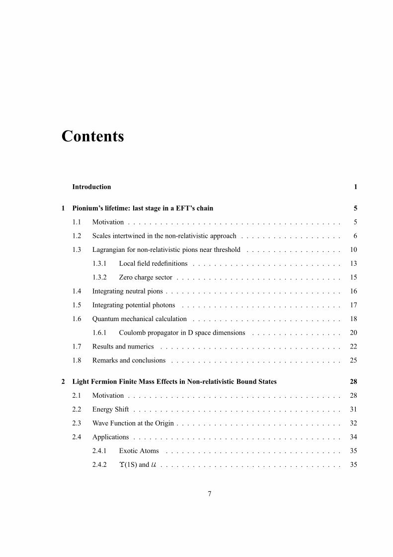
Contents
Introduction 1
1 Pionium’s lifetime: last stage in a EFT’s chain 5
1.1 Motivation . . . . . . . . . . . . . . . . . . . . . . . . . . . . . . . . . . . . . . . . 5
1.2 Scales intertwined in the non-relativistic approach . . . . . . . . . . . . . . . . . . . 6
1.3 Lagrangian for non-relativistic pions near threshold . . . . . . . . . . . . . . . . . . 10
1.3.1 Local field redefinitions . . . . . . . . . . . . . . . . . . . . . . . . . . . . 13
1.3.2 Zero charge sector . . . . . . . . . . . . . . . . . . . . . . . . . . . . . . . 15
1.4 Integrating neutral pions . . . . . . . . . . . . . . . . . . . . . . . . . . . . . . . . . 16
1.5 Integrating potential photons . . . . . . . . . . . . . . . . . . . . . . . . . . . . . . 17
1.6 Quantum mechanical calculation . . . . . . . . . . . . . . . . . . . . . . . . . . . . 18
1.6.1 Coulomb propagator in D space dimensions . . . . . . . . . . . . . . . . . 20
1.7 Results and numerics . . . . . . . . . . . . . . . . . . . . . . . . . . . . . . . . . . 22
1.8 Remarks and conclusions . . . . . . . . . . . . . . . . . . . . . . . . . . . . . . . . 25
2 Light Fermion Finite Mass Effects in Non-relativistic Bound States 28
2.1 Motivation . . . . . . . . . . . . . . . . . . . . . . . . . . . . . . . . . . . . . . . . 28
2.2 Energy Shift . . . . . . . . . . . . . . . . . . . . . . . . . . . . . . . . . . . . . . . 31
2.3 Wave Function at the Origin . . . . . . . . . . . . . . . . . . . . . . . . . . . . . . . 32
2.4 Applications . . . . . . . . . . . . . . . . . . . . . . . . . . . . . . . . . . . . . . . 34
2.4.1 Exotic Atoms . . . . . . . . . . . . . . . . . . . . . . . . . . . . . . . . . 35
2.4.2�
(1S) and �� � . . . . . . . . . . . . . . . . . . . . . . . . . . . . . . . . . . 35
7
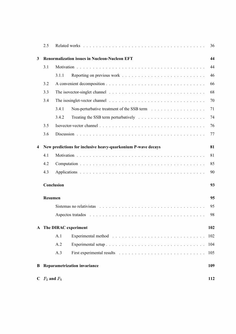
2.5 Related works . . . . . . . . . . . . . . . . . . . . . . . . . . . . . . . . . . . . . . 36
3 Renormalization issues in Nucleon-Nucleon EFT 44
3.1 Motivation . . . . . . . . . . . . . . . . . . . . . . . . . . . . . . . . . . . . . . . . 44
3.1.1 Reporting on previous work . . . . . . . . . . . . . . . . . . . . . . . . . . 46
3.2 A convenient decomposition . . . . . . . . . . . . . . . . . . . . . . . . . . . . . . . 66
3.3 The isovector-singlet channel . . . . . . . . . . . . . . . . . . . . . . . . . . . . . . 68
3.4 The isosinglet-vector channel . . . . . . . . . . . . . . . . . . . . . . . . . . . . . . 70
3.4.1 Non-perturbative treatment of the SSB term . . . . . . . . . . . . . . . . . 71
3.4.2 Treating the SSB term perturbatively . . . . . . . . . . . . . . . . . . . . . 74
3.5 Isovector-vector channel . . . . . . . . . . . . . . . . . . . . . . . . . . . . . . . . . 76
3.6 Discussion . . . . . . . . . . . . . . . . . . . . . . . . . . . . . . . . . . . . . . . . 77
4 New predictions for inclusive heavy-quarkonium P-wave decays 81
4.1 Motivation . . . . . . . . . . . . . . . . . . . . . . . . . . . . . . . . . . . . . . . . 81
4.2 Computation . . . . . . . . . . . . . . . . . . . . . . . . . . . . . . . . . . . . . . . 85
4.3 Applications . . . . . . . . . . . . . . . . . . . . . . . . . . . . . . . . . . . . . . . 90
Conclusion 93
Resumen 95
Sistemas no relativistas . . . . . . . . . . . . . . . . . . . . . . . . . . . . . . . . . 95
Aspectos tratados . . . . . . . . . . . . . . . . . . . . . . . . . . . . . . . . . . . . 98
A The DIRAC experiment 102
A.1 Experimental method . . . . . . . . . . . . . . . . . . . . . . . . . . . . . 102
A.2 Experimental setup . . . . . . . . . . . . . . . . . . . . . . . . . . . . . . . 104
A.3 First experimental results . . . . . . . . . . . . . . . . . . . . . . . . . . . 105
B Reparametrization invariance 109
C � � and � � 112
D Energy Shift and Wave Function correction 114
E The case � � � �116
F Proof of (3.4.1.9) 117
G On � tuning 120
H No continuous solutions of (3.1.1.37) when � 0 124
Acknowledgments 127


Introduction
Effective Field Theories (EFT) furnish us with the technical and conceptual background that
enables the description of the low-energy physics degrees of freedom[1] of a given, interacting system.
They aim at performing a systematic expansion, truncable with a controlled accuracy error, of non-
renormalizable interactions among light modes, that is, those characterized by � � � � � � � � � , where
� is some scale that fixes the frontier for excluded energies (momenta). Information on the heavier
degrees has been integrated out and resides in the couplings of the EFT Lagrangian. That would seem
to indicate that we need, in order to build the Effective Field Theory, the original one as a starting
point. That this is not so becomes one of the main virtues of our framework. An EFT Lagrangian is
constructed, as we will see in the first Chapter, in a general fashion, containing all terms allowed by the
assumed global and local symmetries of our low-energy system, after stating a regularization procedure
and renormalization scheme and having identified a set of small expansion parameters that will allow us
to define a power counting in calculations. This produces the most general S-matrix elements consistent
with analyticity, perturbative unitarity, cluster decomposition and the aforementioned symmetries. So
couplings, those which trace back to the existence of non-included high virtuality states, can be left
as free parameters to be fixed eventually by some convenient set of experiments. If matching cannot
be performed due to its complexity or to our ignorance of the fundamental theory, we still are able to
provide a realistic, sensible and consistently improbable approach to our problem.
Among the variety of fauna that populates the EFT world ( � PT, Electroweak EFT, HQET,
Landau-Ginzburg theory of superconductivity, ... ), our attention will be devoted to the non-relativistic
species (NREFTs, specially worth the accounts in [2]), which was originally proposed by Caswell and
Lepage as the most convenient means of mimetizing particle bound states[3]. In those, the common and
2 Introduction
defining feature is that their relative velocity � comes to be a small parameter. Then � , the mass of at
least one of the particles, belongs to the high-energy domain we do not wish to describe. The explicit
appearance of growing powers of its inverse in the EFT Lagrangian’s coefficients establishes a clear
dimensional ordering for their associated operators. Those theories pervade nature: electromagneti-
cally interacting systems (as positronium ��
� � or muonium ��
� � ), those bound by strong interaction
(heavy quarkonia as �� � , � � � , �� � or �� � ) or formed and decaying by combined mechanisms (hydrogenoid
atoms, pionium �
� ), all of them benefit from the common feature of presenting related and well-
separated energy (momenta) scales whose disentangling can be profited in order to ease the calculation.
Even more, what is an advantage for the non-relativistic EFT formulation, appears as a cumbersome
difficulty that the old approach of a Bette-Salpeter equation with its non-relativistic reduction does not
solve satisfactorily: lack of systematicity, ambiguities and presumptions blur the physical picture.
The calculation of the bound state wave function and its energy levels presents, as a particularity
and main difference with respect to scattering calculations, off-shell initial and final states. The implicit
dependence of these on the interaction coupling constants ( � � � ) results in a non-trivial choice of order-
by-order in � � � contributions from different sorts of Feynman graphs. To be more specific, the leading
order in � � � does not follow from the number of vertices in the diagrams and it becomes completely
unavoidable to resum an infinite series of them (for instance ladder photons in QED) in order to provide
the leading order approximation. After doing so no spurious, gauge dependent terms, generated at every
order in � and cancelled in the resummation, will arise.
As we see, the problem lies on the existence in these diagrams of different hierarchically or-
dered physical scales entangled and contributing. For example, in NRQED those would be the mass �
of a heavy particle, that is larger than the relative momentum � � � � of the bound state, which at the
same time is larger than the bound state energy � � � � � ( � � ��). In HQET we would have only the
scale � which is larger than � � � � and � � � � � � � � . A non-relativistic EFT organizes itself as to
power count correctly, so taking as starting point the evaluation of the non-relativistic Green function
through a Schr �� dinger equation. Corrections coming from retardation or non-potential effects (given by
interacting low-energy particles), relativistic effects (expansion of �� in the energies and wave function)
and higher order perturbative interactions, not only enter consistently at every stage of the calculation
but are also incorporated in such a way that no unwanted IR divergences arise, UV divergences are per-
Introduction 3
turbatively renormalized by the couplings at our disposal, non-perturbative contributions of the theory
(read here QCD) are isolated and parametrized ...
But NREFTs do not restrict themselves to implementing technical facilities. They also broaden
our knowledge about some conceptual issues. For example, we will see in the following pages that,
once � has been integrated, we might take the NR formulation to a potential level whether it is the
case that � � can also be integrated. This last step gives rise to the appearance of potentials as matching
coefficients, so paving the way from a Field Theory formulation to a Quantum Mechanical setting.
In such spirit, this work is intended to be, more than a collection of different calculations per-
formed in the common framework of NREFTs, my own learn-it-on-the-way report where every chapter,
when focusing on a small range of theoretical aspects tightly related with problems of present concern
in the field, reinforces the impression of unity. Besides providing answers to phenomenologically rel-
evant questions, this set of contemporary examples aims at reviewing fundamental building blocks of
NREFTs. So, in the first chapter, while tackling the calculation of pionium’s -electromagnetically, loose
bounded ��
and � � system- decay, we gaze at the importance of different, more or less widely ranged,
energy and momentum scales that give rise to a series of NREFT’s Lagrangians, also characterized
by their symmetries and counting rules, which constitute intermediate stages in the way to a quan-
tum mechanical formulation. Other issues such as reparametrization invariance and field redefinitions,
matching calculations and accuracy control, also enter our scope and are emphasized.
The second chapter, concerning the finite mass effects of vacuum polarization corrections in
non-relativistic bound states, puts the stress on the integration of competing physical scales and on
different fields of applicability of one and the same calculation.
The third section offers a brief review and our own approach to one of the issues that has become
more controversial in the last years and has moved to considerable, and perhaps not enough rewarded,
effort: that is, renormalizability in the context of Nuclear Physics EFTs and, to be more concrete, in
NN interaction.
Finally, the last chapter is devoted to the calculation of the P-wave decays of heavy quarkonium.
Potential Non-Relativistic QCD (pNRQCD), the ultrasoft EFT of a soft one, (the so-called NRQCD),
will enable us to write the NRQCD colour-octet matrix elements in terms of derivatives of wave func-
tions at the origin and non-perturbative universal constants. Thanks to this, we achieve a new set

4 Introduction
of relations among hadronic inclusive decays’ branching ratios for quarkonia with different quantum
number and with different heavy flavour.
Chapter 1
Pionium’s lifetime: last stage in a EFT’s
chain
1.1 Motivation
The striking simplicity of organizing corrections to one process and non-model dependency of
calculations undertaken in NREFTs is perfectly well displayed in the following pages, that aim at offer-
ing a clear derivation of the ��
� � (pionium) loosely, electromagnetically bounded ground state decay
rate to neutral pions with a precision of 10%. This high accuracy is to be expected in DIRAC’s experi-
ment (see Appendix A), currently performed at CERN[4], so that theoretical predictions will be sternly
tested and the nature of spontaneous chiral symmetry breaking will receive further enlightenment. Be-
ing pionium’s lifetime proportional to the square of the difference between the strong scattering lengths
for isospin 0 and 2, � � - � � , whose value is predicted to be, in the framework of Standard Chiral Per-
turbation Theory, equal to .265�
.004, any discrepancy coming from experimental values would signal
the relevance of a Generalized Scenario[5] (where � � - � � is fitted to .29 from � � decays and � � phase
shifts).
It is of general knowledge that in the chiral limit where � � � � � � � � = 0, QCD’s flavour
symmetry � � � � � � � � � � � � � is spontaneously broken down to � � � � � � , so arising eight massless Gold-
stone bosons coupled to the conserved axial-vector currents[6]. In the real world, where light quarks
have small masses (in comparison with the typical hadronic mass scale � � � 1 GeV.) this approximate
6 Pionium’s lifetime: last stage in a EFT’s chain
symmetry serves us to establish � PTh, the low-energy effective theory obeyed by Goldstone bosons,
as a systematic expansion in powers of external momenta and quark masses. Nevertheless, the usual
assumption that the quark condensate mechanism is dominant as a symmetry breaking effect is some-
what controversial. It still holds the possibility that, instead of the Standard value of 2 GeV. ( �� ��
� � � )
for the quark condensate order parameter,� �
� � � �
� � � �
� �� , the rather lower value �� � �
MeV. suits,
so giving consistency to a less constricted picture that is called Generalized � PTh. The latter departs
widely from Standard counting rules1 :
�� � � � �
� � � � ��
� ��
� ��
�
!� � � � �
� � � � � � ��
� � � � � (1.1.1)
enlarges the number of parameters needed in order to calculate to a given order2 and grants flexibility.
For instance, the ratio # �� %&� , ( '� �
� ) � � *� ), which has a definite value � 26 in Standard � PTh, can
oscillate between 6.3 (8 when including higher order corrections) and 26 in the Generalized Scenario.
Implications for the temperature of the Chiral Transition are exhibited in the following figure. Notice
that S � PTh predicts � , � 200 MeV. whereas G � PTh would allow for a smaller value.
1.2 Scales intertwined in the non-relativistic approach
After pionium atoms were first observed in the late eighties[10] and the interest of measur-
ing their lifetime became evident[11], propelled by DIRAC’s high precision intended measurement,
several papers tackling with such a calculation have appeared, showing the compelling necessity of a
model independent, systematic method. So, first attempts in this direction, relativistic potential mod-
els where the strong interaction was modeled by square wells and the electromagnetic interaction was
preliminary switched off to provide for a way of comparison with the purely hadronic situation, lacked
completely from any of those desirable characteristics[12]. The situation was somewhat improved em-1Somewhat restricting this counting to the case where the bilinear condensate - vanishes in the chiral limit, the authors
of [7] have identified a pattern of Chiral Symmetry Breaking ( . SB) where the Generalized Scenario is self-consistent. There,a custodial discrete subgroup / 1 of the axial 2 3 4 6 7 9 survives, so precluding the formation of a bilinear condensate, whilethe allowed quartic condensates become the natural order parameters. Regretfully, although this realization of . SB is notruled out in gauge theories with scalar quarks and/or Yukawa couplings, it does enter in direct contradiction with exact QCDinequalities[8].
2Take the : < 4 > 9 A B : < 4 > 9 D realization of . PT, where properties of pions are calculated. There the Generalized Scenariobuilds on the basis of a value of the effective coupling E G which is completely unnatural from the Standard point of view.

1.2 Scales intertwined in the non-relativistic approach 7
1015
2025
r
50
100
150
200
250
Temperature �MeV�
0
1003
2003
3003
�q���q� �MeV�3
1015
2025
Figure : Quark condensate versus temperature and r [9].
ploying two-body wave equations of 3D constraint theory[13] and field theoretical approaches based
on the Bethe-Salpeter equation[14]. Nevertheless we can state that the major breakthrough came by the
hand of the non-relativistic EFT approach[15, 17, 18], that combined efficiency and simplicity with the
abovementioned features.
Why a non-relativistic calculation is suited to our problem is well-understood once we assign
numbers to the different energy-momentum scales involved in the lifetime. Pionium decays mainly by
strong interaction to two neutral pions. In first approximation its associated lifetime is given by Deser’s
formula[19]:
�� � � �
� ���
���
� � � � � � � � � � �
�� � � � � � �
�� (1.2.1)
whose derivation we will review when calculating its corrections, in the next few sections. Three
physical scales appear in this expression: the higher one, � � � 140 MeV. will be in the following the
mass of the charged pions; � � � 5 MeV. designates the mass difference between charged and neutral
pions, � � � � � � � , with associated non-relativistic momentum � � � � � 40 MeV.; the lower one is
the inverse of the Bohr radius, which appears through the wave function at the origin,� �
� � .5 MeV.
They all combine to give a value� � �
� � � � .2 eV., where we have used the leading order value for the
difference between isospin 0 and 2 scattering lengths (� �
�� � ��), as calculated from the � -Lagrangian.
�� � �
is then, a quantity of order � � . The next relevant decay channel, ��
� � � � � , counts at leading order
8 Pionium’s lifetime: last stage in a EFT’s chain
as�
� � =� � �
� and therefore it can be safely ignored at the 10% accuracy level.
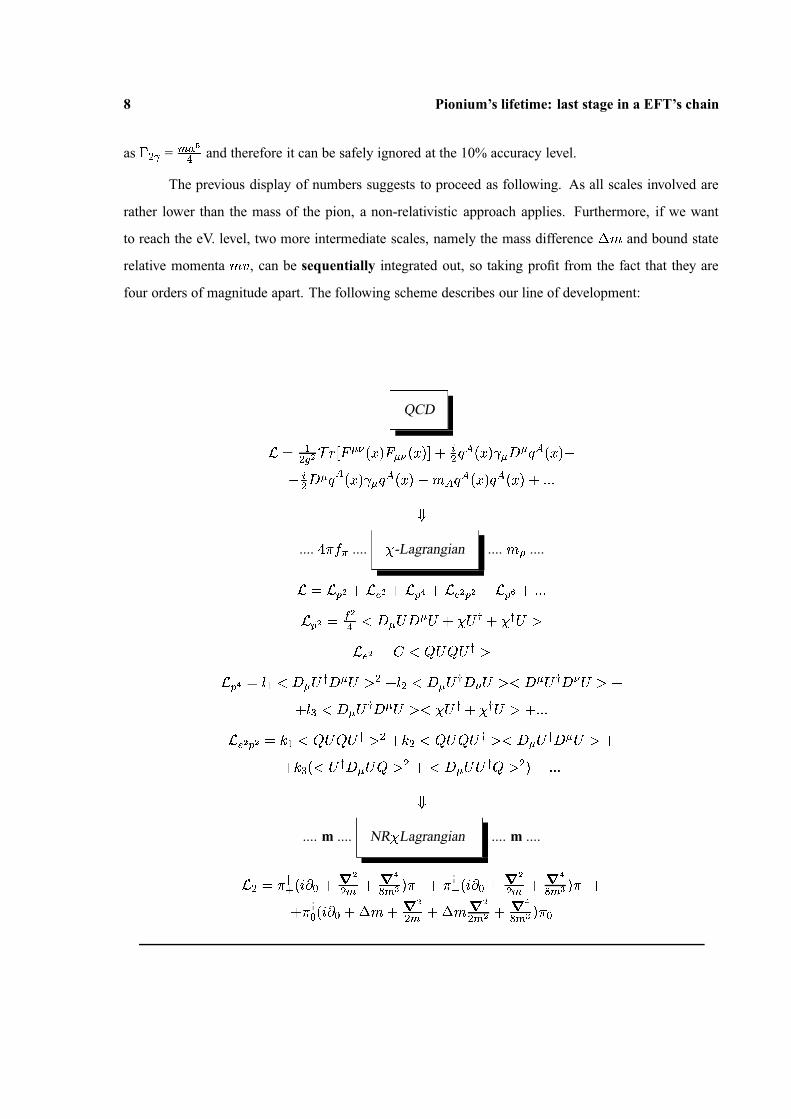
The previous display of numbers suggests to proceed as following. As all scales involved are
rather lower than the mass of the pion, a non-relativistic approach applies. Furthermore, if we want
to reach the eV. level, two more intermediate scales, namely the mass difference � � and bound state
relative momenta � � , can be sequentially integrated out, so taking profit from the fact that they are
four orders of magnitude apart. The following scheme describes our line of development:
QCD
��
�
� � � � � � � � � � � � � � � � � �� �
� � � � � � � � � � � � �
� �� �� � �� � � � � � � � � � � �
�
� � � � � � � � � � � � � �!
.... " � # � .... � -Lagrangian .... � % ....
��
� '� � � )
� � � ' , � � )�
'� � � ' - � � � �
� '� �
� �
� � � 0 � 0 � � 01 � �
10 3� )
� � 6 � 8 0 8 01
3� ' ,� 9 � � � 0
1� 0 3 � � 9 � � � 0
1� � 0 3 � � 0
1� � 0 3 �
� 9 � � � 01
� 0 3 � � 01 � �
10 3 � � � �
� )�
'� � @ � � 8 0 8 0
13 � � @ � � 8 0 8 0
13 � � 0
1� 0 3 �
� @ � � � 01
� 0 8 3 � � � � 0 01 8 3 �
� � � � �!
.... m .... NR � Lagrangian .... m ....
�� � �
1� � C E � � G �
� � � G,
� � � � � � � �1
�� C E � � G �
� � � G,
� � � � � � �� �
1� � C E � � � � � G �
� � � � � G �
� � � � G,
� � � � � �
1.2 Scales intertwined in the non-relativistic approach 9
�� � � � � �
�� �
�� � � � � � � � � �
�� �
��
� � � � � � � � � ��
� ��
� � � � � � � � � � � �� �
� � � ��
� ��
� � � � �� � � � � � � � � �
� ��
��
� ��
�� � � � �
� � � � � � �� � � � � � � � � �
� �� �
��
�� �
�� � � � � �
� � � � � � �� � � � �
��
� ��
�� � � �
� � � � � � � � �� � � � �
�� � �
�� � � � � � � � � � � �
�� � �
��
� � � � � � ���
� ��
� � � � � � �
�
.... � � .... NR � Lagrangian (only charged sector) .... ��
� � � ....
� �� �
�� � � � � � � �
� � � � � � ���
� � � � � � �� � � � � �
� ��� � �
�� �
��
� � � � � � ��
�� �
��
� � � � � ��
.... � �� .... pNR � Lagrangian .... � � ....
�� �
�� � �
�� � � � � � �
� � � � � � ��
� � ��
�� �
�� � � � � � �
� � � � � � ��
� �� �
�� � � �
�� �
��
� � � � � � ��
� � ��
� ��
� ��
�� � �
�� � � � � � � � � � �
�� �
� � � � �� �
�� � � � � �
��
� �� � � �
�� � �
�� � � �
�� � � � �
��
� � � ��
��
��� � � �
�� � � �
�� �� � �
�� � � � �
�� � � � � � �
� � �� � �
� � � � � � � �� �
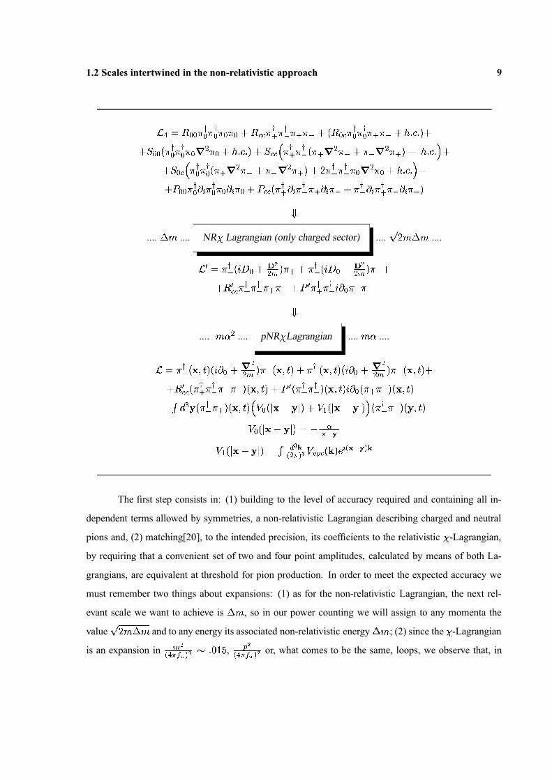
The first step consists in: (1) building to the level of accuracy required and containing all in-
dependent terms allowed by symmetries, a non-relativistic Lagrangian describing charged and neutral
pions and, (2) matching[20], to the intended precision, its coefficients to the relativistic � -Lagrangian,
by requiring that a convenient set of two and four point amplitudes, calculated by means of both La-
grangians, are equivalent at threshold for pion production. In order to meet the expected accuracy we
must remember two things about expansions: (1) as for the non-relativistic Lagrangian, the next rel-
evant scale we want to achieve is � � , so in our power counting we will assign to any momenta the
value ��
� � � and to any energy its associated non-relativistic energy � � ; (2) since the � -Lagrangian
is an expansion in� ��
� � � � � � � � � �,
���
� � � � � or, what comes to be the same, loops, we observe that, in
10 Pionium’s lifetime: last stage in a EFT’s chain
principle, one should expect only the � -Lagrangian to one-loop order to be relevant (therefore, only � � ,
� � � � effects would be taken into account, if we use the standard counting � � �� ��
� � � � � � ). Nevertheless,
series do not converge so quickly. We further qualify in that respect in the future.
Next stage take us down to a Lagrangian which does not contain neutral pions. By integrating
out the scale � � imaginary parts are generated and coefficients inherit series in� � �
� ��
� . As this
quotient is � ��, it is required to keep second order corrections in this variable.
Eventually, we reach the relative momentum scale. Coulomb photons are resummed and pio-
nium is formed. Coefficients turn out to be potentials and calculations in this theory reduce to Quan-
tum Mechanical ones. When computing, it is expected to find, besides the previous quotients and as
most relevant contributions from the last integration performed, relevant corrections in � and some in� � ��
� � � � �� �
� � which will be beyond our scope.
1.3 Lagrangian for non-relativistic pions near threshold
We shall start by writing down the non-relativistic Lagrangian which, organized in powers of �� , serves
us to describe the dynamics of a two pion system whose off-shell energy is well below � . The next
relevant scales for the problem at hand, that is, � � for the energy and ��
� � � for its associated
momentum, provide an estimation of the size of every operator and allow us to stop the expansion of
the Lagrangian at the appropriate level of accuracy.
In constructing this Lagrangian attention must be payed on the symmetries (exact and approxi-
mate) inherited from the fundamental theory, in our case from the � -Lagrangian. Being � an integrated
scale, our most characteristic internal symmetry, the chiral one, enters only through the parameters
of the Lagrangian, which might be expanded in powers of� �
� � � � �
. No further algebraic implications
constrain from this side the form of the theory.
On the contrary, isospin, the approximate internal symmetry explicitly broken by up and down
quark mass difference, � � � � � , and electromagnetic interactions, generates the neutral to charged pion
mass gap � � � � � � , still a small quantity. Hence isospin symmetry is a good (approximate) symmetry
for the non-relativistic Lagrangian. In order to implement it we shall use the vector � , defined as:
� ��
� � � � ��
� �� � � � �
��
�� � � � � (1.3.1)

1.3 Lagrangian for non-relativistic pions near threshold 11
where � � , � � and � � annihilate positive, negative and neutral pions respectively, as well as the � � -
proportional vectors � � ��
��
� � � and � � ��
��
� � � � � � � , that take into account isospin breaking
effects due to electromagnetic and strong interactions.
As for space-time and discrete symmetries, they are implemented in the standard way. In par-
ticular, the Lorentz subgroup requires the introduction of a non-linear implementation equivalent to
imposing the so-called reparametrization invariance (see Appendix B), that turns out to be quite simple
in the case of spin zero fields. That is, consider a composite spin zero field made up of tensor products
of � � and � ��
and define � � � � � as the weight of the field. If � ���, then all derivatives acting
on the field must be introduced through the combination:
� � � � � ��
�
� �� � � � � (1.3.2)
If � ��, we are allowed to act with � � on this field. Then all Lorentz indexes in the Lagrangian will
appear contracted in a formally Lorentz invariant way. � must be considered a Lorentz invariant on its
own.
With this simple rules in mind and considering in first place the limit of exact isospin symmetry,
the following terms must be incorporated in the non-relativistic Lagrangian:
�
�
� �
� �
�� �
� � � �� � � � �
� �
� � � �� �
� � �� � � � �
�� �
� � ��
� � �
� � �� � �
� �� �
� � �
� � � �� �
�� � �
�� �
� �� � � � � � �
��
�� �
�� � �
� ��
� � � � � � � ��
��
� � � � � �� � �
�� � � � �
�� � � � � �
�� � �
��
�� � � � � � �
� � � � ��
� � � � � ��
� � � �
� �� � �
� �� � � � � �
�� � (1.3.3)
Previous constants contain also information on isospin conserving electromagnetic interactions,
both at quark level and those newly entering by matching from the relativistic Chiral Lagrangian. As
for isospin breaking pieces, they are incorporated by making use of the previously introduced vectors

12 Pionium’s lifetime: last stage in a EFT’s chain
Q and M. Regarding that due to charge conjugation � � � � � contributions enter quadratically and
are small[21] ( � .1 MeV., charged to neutral pion mass difference is mainly an electromagnetic effect),
in the future we will ignore terms involving M. Remembering that Q must always appear in pairs, we
include the following invariants in our Lagrangian:
��
� ��
� � ��
� �
��
� � �� �
� �� � �
� � � �� �
��
� � �� �
� � � �� �
�� �
� �� � � � � �
�� � � � � � �
�� � � �
� � � � � ��
� � � � � � � �
�� �
� � � �� � � � � � � � � � � � � �
��
�� � � � � � � � � � � � � � �
�� � � �
�� � �
� � � � � ��
�� � � � �
� � (1.3.4)
Before going on, let us discuss the general structure of the constants�
,�
, � and � above. Calling�
to any such a constant and � to its dimension, then the general form of�
will be:
�� � �
��
�� � � �
��
� � � �
� � ��
�
� � � �
� � �
��
� � � �� � � �
� � � � � � � � (1.3.5)
� � � � ��
�
� � � �
� � � � ��
�
� � � �
� � � � � � (1.3.6)
� , i=0,1,..., refers to pure strong interactions. Spontaneous chiral symmetry breaking implies that only
those constants accompanying bilinear terms, that is�
� and � , can have ��
� ���, as in the limit � �
pions become free particles as regards to strong interactions. The subindex numbering keeps track of
the higher number of loops that contributes to each four-boson term and, as you see, we have stopped
at two loop order[22], which is the present stage of calculations. � � combine leading electromagnetic
with strong interactions[23]. As our future expressions will not make use of this chiral expansion, they
contain in principle all number of loops. Nevertheless, let us mention for numerical purposes that the
previous series, although displayed in terms of� �
� � � � �
, are seen to converge (that is, they have � ��
coefficients) better as� �
� � � �
. To one loop order we have 20% corrections. To two loop order 5%.
Although right now this is superfluous information, let us advance that, from final expressions, it is
clearly observed that the 10% aimed accuracy require one combination of the above constants, that
1.3 Lagrangian for non-relativistic pions near threshold 13
enters quadratically in Deser’s formula, to be provided at two loop level. Therefore, matching with
� PTh involves� �
� ,� � �
,� � �
and�
��
� ,�
�� �
, if we keep counting �� as standard �
� �� � � � �
.
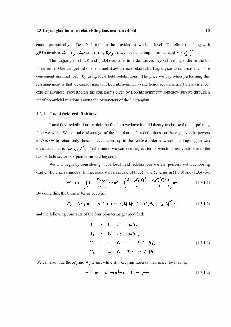
The Lagrangian (1.3.3) and (1.3.4) contains time derivatives beyond leading order in the bi-
linear term. One can get rid of them, and draw the non-relativistic Lagrangian to its usual and more
convenient minimal form, by using local field redefinitions. The price we pay when performing this
rearrangement is that we cannot maintain Lorentz symmetry (and hence reparametrization invariance)
explicit anymore. Nevertheless the constraints given by Lorentz symmetry somehow survive through a
set of non-trivial relations among the parameters of the Lagrangian.
1.3.1 Local field redefinitions
Local field redefinitions exploit the freedom we have in field theory to choose the interpolating
field we wish. We can take advantage of the fact that such redefinitions can be organized in powers
of � � � � to retain only those induced terms up to the relative order at which our Lagrangian was
truncated, that is � � � � � ��
� . Furthermore, we can also neglect terms which do not contribute to the
two particle sector (six pion terms and beyond).
We will begin by considering those local field redefinitions we can perform without loosing
explicit Lorentz symmetry. In first place we can get rid of the�
� and � � terms in (1.3.3) and (1.3.4) by:
� �� � ��
� ��
�� � � � � � � � � ��
� � � �� �
� � � � �� � � � (1.3.1.1)
By doing this, the bilinear terms become:
�� � � �
� � � �� � � � � � � � � � � � � � � �
�� � � � � � � �
� � � (1.3.1.2)
and the following constants of the four pion terms get modified:�
� �� �
� ��
� ��
�
�� �
�� �
� �� �
�� �
��
�� �
� � � � � �� � � � � � � � � � �
�� �
�� � (1.3.1.3)
� � � � � �� � � � �
�� � � � � �
�� �
��
We can also hide the� �
� and� �
� terms, while still keeping Lorentz invariance, by making:
� �� � �� �
� � � � � � � � �� �
� � � �� � � � � (1.3.1.4)

14 Pionium’s lifetime: last stage in a EFT’s chain
which induces:
�� �
� � �� � �
� � �� �
� �� �
� � � �
�� �
� � �� � �
� � �� �
� � �� �
� �� �
� � � � � � (1.3.1.5)
The remaining time derivatives in � and in the�
� and�
� terms can only be removed if we
give up the explicit realization of Lorentz symmetry which we have kept so far. Notice that the time
derivatives in the�
� term are higher order and can be dropped. Higher order time derivatives in the
bilinear terms are removed by:
� � �� � � ��
� �
�� �
�
�� �
� � ��
�� � � � � �
�� �
� � (1.3.1.6)
Finally the time derivatives induced by this redefinition in the four pion terms together with the remain-
ing time derivatives in�
� and�
� can be absorbed in:
� �� � �� �
��
�
�� � � � � � � � � �
� ��
�
��
�� � � �
� � � � � (1.3.1.7)
In this way we obtain finally the Lagrangian in its minimal form:�
��
� � �� �
�� � � � � � � � � � � �
�
�� �
�� �
� � � � � � � � �
�
� �� � �
� � � �� �
� � � �
�� �
�� � � � � �
� � �� � � � � � � � � �
� � � � � � � �
��
� � � �
��
� � � � � � � � � (1.3.1.8)
� � �
� � � �
��
� � � � � � � � � � � � �
��
� � � � � � �� � � � � � � � � � � � � �
� � �� � � � � � � � � � � � � �
� � � � � � � � �� � � � � � � �
� � � � � � � �� � �
� � � ��
� � � � � � ��
�� � � � � �� �
��
� � � � �� �
�� � � � � � � � �
��
� � � � � � �
where coefficients � � , � � , � �� and � �
� are related with those from (1.3.3) and (1.3.4) by:
� � � � � � � � � ��
� ��
� � � � � � ���
� � � ��
� � ��
��
�� � � �
��
� �
� � ��
�
��
�� � (1.3.1.9)
� �� � � � �
�� � � �
� ��
��
�� �
�� � � �
��
� � � � �
� �� � � � �
� �� � � �
� � ��
��
�� �
� �� � � ��
�� �
� � � � � � �

1.3 Lagrangian for non-relativistic pions near threshold 15
Lorentz symmetry guarantees that the bilinear terms have the standard form including relativis-
tic corrections. It also relates�
� and� �
in the two last terms to the remaining constants. Unfortunately,
as these coefficients introduce terms related to the center of mass momentum, which is irrelevant to our
problem, these relations have no practical consequences.
1.3.2 Zero charge sector
The zero charge sector in terms of the pion field reads:
�� � �
�� � � � � �
�
�
�
� �
��
�� � � � �
��
� � � � � �
�
�
� �
��
�� � � �
� ��
� � � � � � � � � �
��
� � � �
��
� � �
��
�� � � �
�� � � � � �
�� �
�� � � � � � � � � �
�� �
��
� � � � ��
� � � ��
� ��
� � � � � � � � � � � � (1.3.2.1)
� �� �
��
�� �
�� � �
�� � � � � � � � � � � � �
��
� ���
�� �
�� � � � �
�� � � � � � � � � �
� �� � �
��
� ��
�
�� � �
� � � � � �� � � � �
��
� ���
� � �� � � � � � � � �
� � � � ��
� � � ��
� � � � � � � � � � ��
��
� � � ���
� � � � � � � ��
�� � �
�� � � � � � � � �
whose constants are defined as:
� � � ��
� � �� � �
�� � �
� � � �� � � � �
� � �� �
� � � �� �
� � ��
� � �� � �
� � � �� �
� � � �� � �
�� � � �
�� � � � ��
�� � ��
�� (1.3.2.2)
�� � � � ��
��
� � � � � ���
� � �
��
� � � �� �
� �
� � � �� �
� �
Notice that since the origin of energies appears to be at the two charged pion threshold, the neutral pion
shows a negative energy gap � � � ��. These terms in the Lagrangian can be combined in a more
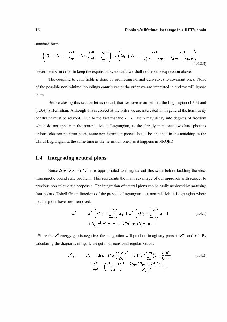
16 Pionium’s lifetime: last stage in a EFT’s chain
standard form:
� � � � � � � � � �
��
� � �� �
��
� � � �
��
�� � � � � � � � � � � �
�� � � � � �
� � �
�� � � � � � �
� �(1.3.2.3)
Nevertheless, in order to keep the expansion systematic we shall not use the expression above.
The coupling to e.m. fields is done by promoting normal derivatives to covariant ones. None
of the possible non-minimal couplings contributes at the order we are interested in and we will ignore
them.
Before closing this section let us remark that we have assumed that the Lagrangian (1.3.3) and
(1.3.4) is Hermitian. Although this is correct at the order we are interested in, in general the hermiticity
constraint must be relaxed. Due to the fact that the ��
� � atom may decay into degrees of freedom
which do not appear in the non-relativistic Lagrangian, as the already mentioned two hard photons
or hard electron-positron pairs, some non-hermitian pieces should be obtained in the matching to the
Chiral Lagrangian at the same time as the hermitian ones, as it happens in NRQED.
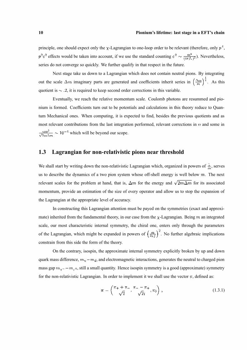
1.4 Integrating neutral pions
Since � � � � � � � it is appropriated to integrate out this scale before tackling the elec-
tromagnetic bound state problem. This represents the main advantage of our approach with respect to
previous non-relativistic proposals. The integration of neutral pions can be easily achieved by matching
four point off-shell Green functions of the previous Lagrangian to a non-relativistic Lagrangian where
neutral pions have been removed:
� �
� �
� � � � � � ��
��
� � � � � �
� � � � � ��
��
� � � � (1.4.1)
� ��
� � �
� �
�� � � � � �
�
�
� �
�� � � � � � � �
Since the � � energy gap is negative, the integration will produce imaginary parts in ��
� � and ��
. By
calculating the diagrams in fig. 1, we get in dimensional regularization:
��
� � � � � � � � � � � �� � � �
�� ��
�� �
� � � � � � �� � ��
�
� � ���
� �
� � � (1.4.2)
� �
�� �
� � �� � � � � ��
�� �
�� �
� � � � � � � � �� � � � �
� � � � � � � �

1.5 Integrating potential photons 17
��� �
� �
� �
��� �
��� �
� �
� ��
�� �
� �
� �
��� �
� �
� ��
�� �� �
� �
� �
� �
��� �
� �
� �
��� �
��� �
� �
� �
��� �
��� �
� �
� �
��� �
Figure 1: Diagrams contributing to the matching between � and � � up to corrections � � � � � � � � . No dec-orated vertices belong to � � � insertions. � corresponds to a � � � interaction; � indicates a relativistic correctioncoming from � ! " � $ ; % one of � � � ( � � type.
��
� � � � � � �� �
�
� � �
� (1.4.3)
where � � ��
� � � . ��
� � and � �
contain the leading corrections in � � � � and � ��
� � � � respec-
tively. The electromagnetic contributions to )�
coming from the energy scale � � are negligible, as well
as the relativistic corrections � � ��
��
� to the charge pions and the terms � � � and� � � in (1.3.2.1).
1.5 Integrating potential photons
The Lagrangian in the previous section is almost identical to NRQED (for spin zero particles)
plus small local interactions. In refs. [24] it was shown that we can integrate out the next dynam-
ical scale, namely, � � ��
in NRQED obtaining a further effective theory called potential NRQED
(pNRQED), whose coefficients include the usual potential terms, where only the ultrasoft degrees of
freedom ( � � ��
� � ) remain dynamical. We shall do the same here.
The (maximal) size of each term in (1.4.1) is obtained by assigning � � to any scale which is
not explicit. Apparently no corrections in � � � � to the Coulomb potential arise, since tranverse photons
start contributing to � � ��
� , which is beyond our present interest. However, as pointed out in ref. [27],
below the pion threshold there are further light degrees of freedom apart from the photon. In particular,
the electron mass ��
is � � � ��
and hence it must be integrated out here. This gives rise to a potential
18 Pionium’s lifetime: last stage in a EFT’s chain
��
� �
��
� �
��
� �
��
� �
��
� �
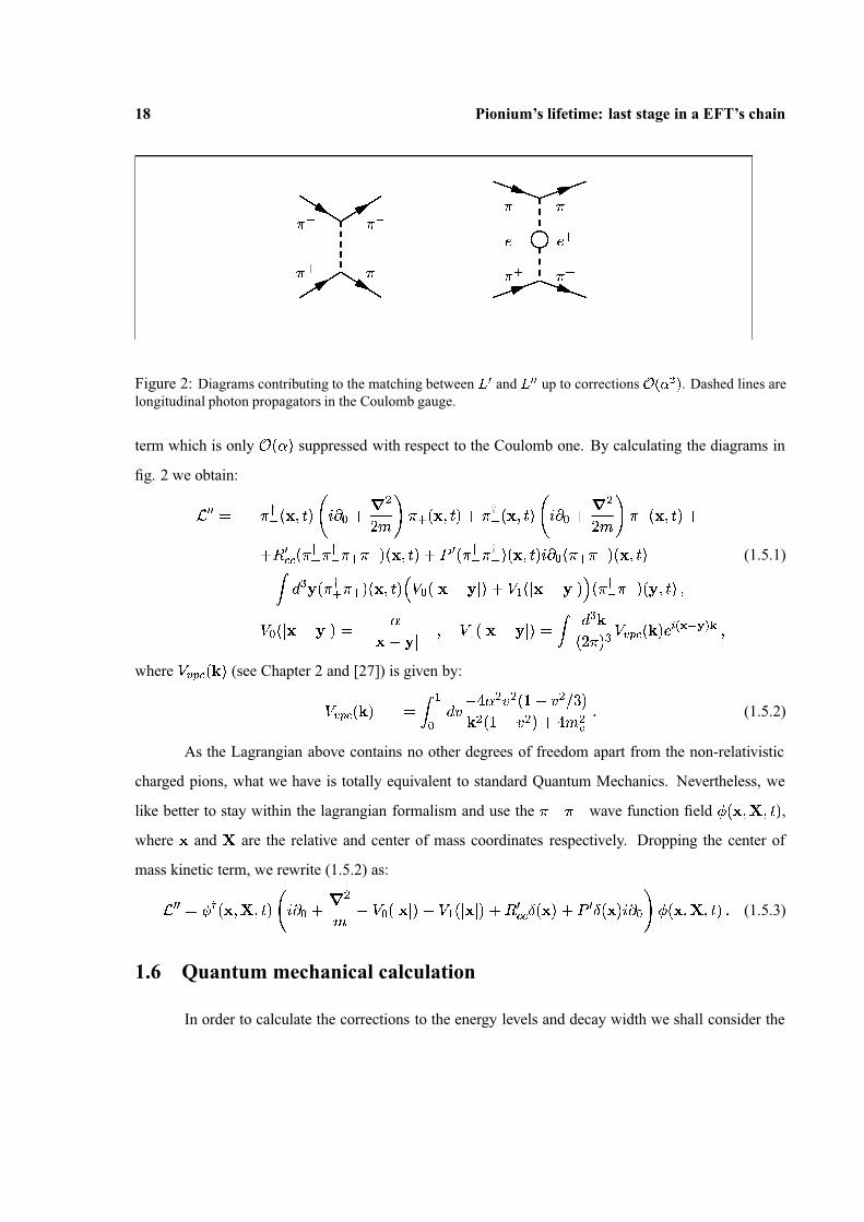
Figure 2: Diagrams contributing to the matching between � � and � � � up to corrections � � � � � . Dashed lines arelongitudinal photon propagators in the Coulomb gauge.
term which is only � � � � suppressed with respect to the Coulomb one. By calculating the diagrams in
fig. 2 we obtain:
� � �
� ��
� � � ��
� � � � � � ��
�
�� � � � � �
�� � �
��
� � ��
� � � � � � ��
�
�� � � � � �
�� �
� ��� � � �
�� �
��
� � � � � � � ��
� � ��
� ��
� ���
� � � ��
� � � � � � � � � � � � ��
� � (1.5.1)
�
� � � �� �
�� � � � � � �
��
� �� � � � � �
� � � �� � � � � �
� � � ��
�� � � �
��
�� �
�� � � � � �
� � � � �� � � �
��
�� � � � � �
� � �� � �
��
� � �
� � �� � � � � �
� � � ��
where� � �
� � � (see Chapter 2 and [27]) is given by:� � �
� � � �� �
�
� �� � � � � � �
� � � � � � �
� �� � � � � � � � �� (1.5.2)
As the Lagrangian above contains no other degrees of freedom apart from the non-relativistic
charged pions, what we have is totally equivalent to standard Quantum Mechanics. Nevertheless, we
like better to stay within the lagrangian formalism and use the � � ��
wave function field � � � � � ��
� ,
where � and � are the relative and center of mass coordinates respectively. Dropping the center of
mass kinetic term, we rewrite (1.5.2) as:
� �� � �
� � � � ��
� � � � � � �
��
�� � � � � � �
�� � � � � � � �
�� � � � � � � �
�� � � � � � � � � � � � �
�� (1.5.3)
1.6 Quantum mechanical calculation
In order to calculate the corrections to the energy levels and decay width we shall consider the
1.6 Quantum mechanical calculation 19
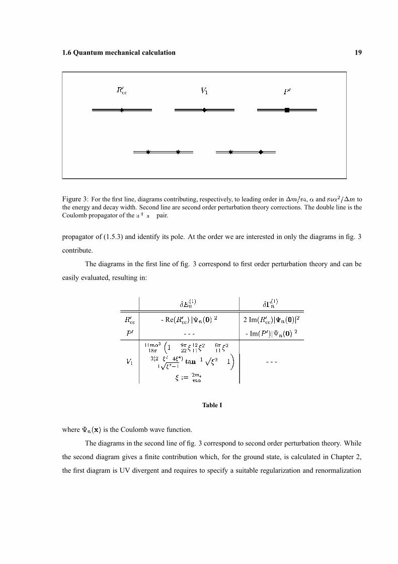
��
� ��
� ��
Figure 3: For the first line, diagrams contributing, respectively, to leading order in � � � � , � and � � � � � � tothe energy and decay width. Second line are second order perturbation theory corrections. The double line is theCoulomb propagator of the � � � � pair.
propagator of (1.5.3) and identify its pole. At the order we are interested in only the diagrams in fig. 3
contribute.
The diagrams in the first line of fig. 3 correspond to first order perturbation theory and can be
easily evaluated, resulting in:
� �� � �� �
� � � ���
�� � - Re � �
�� � � � � � � � � �
� 2 Im � ��� � � � � � � � � �
�
��
- - - - Im � ��
� � � � � � � ��
� � � � ��
� � ��
� �
� � �
� �� � �
� � �
� � ��� � �
��
� ��
� � �
� � � ��
� � � � �� � � � � � � - - -
� �� � � �
� �
Table I
where � � � � � is the Coulomb wave function.
The diagrams in the second line of fig. 3 correspond to second order perturbation theory. While
the second diagram gives a finite contribution which, for the ground state, is calculated in Chapter 2,
the first diagram is UV divergent and requires to specify a suitable regularization and renormalization

20 Pionium’s lifetime: last stage in a EFT’s chain
� PTh � � pNR � PTh
��
� � � �
�� �
�
� �
��
� �
��
� �� �
�
� �
Figure 4: IR divergent relativistic diagram of order � � � � in � PTh matches a delta type interaction in pNR � PTh.
scheme. The subtraction point dependence of the result will eventually cancel against those contained
in the matching coefficients. Down from the Chiral Lagrangian, ��
� � inherits by the matching procedure
an IR factorization scale that has been introduced through the calculation of the next figure’s divergent,
two loop diagram calculated at threshold in � PTh.
Both, the IR divergent previous diagram and the Quantum Mechanical UV divergence, must
be regularized and renormalized using one and the same scheme, most efficiently in DR with � �(or
� �). That is what we have done with this first diagram of fig. 3, briefly sketched in next subsection.
1.6.1 Coulomb propagator in D space dimensions
First diagram in fig. 3 is given once we know�
� � � � � � � � , the Coulomb propagator at threshold
in D (= 3+ 2 ) spatial dimensions. Although for the actual Coulomb potential in D dimensions:
�� � � � � �
� � �
� � � � � � � �� �
� � �� �
� � ��
��
�
�� (1.6.1.1)
we were not able to find an explicit representation, a slight modification of it:
� �� � � � � �
� ��
��
� ��� �
� �� � � � �
� � � � � � � �
�� (1.6.1.2)

1.6 Quantum mechanical calculation 21
��
� � � �
�� �
�
� �
Figure 5: Logarithmically divergent diagram which is calculated with the two longitudinal photon propagators(1.6.1.4) for the dashed lines.
admits the following exact representation, which is a generalization of that presented in ref. [25]:
� �
� � � ��
� � � �
��� � �
�� � � � � � � �
�� � �
� � �� �
��
� ��
� � ��
�� � �
� �� � � � � � � � � � � �
�
� �� � �
��
� � ��
��
� � ��
� � � � � � � � ��� � �
�� � � � � �
� ��
� � � �� � � � � �
� ��
� � ��
� � ��
��� � � � � � � �
� �� �
� � ��
� � �� � �
�� � � �
��
�
(1.6.1.3)
where � � �
� are the spherical harmonics in � dimensions and � � � � � � � .
The potential� �
� � � � corresponds to the following modification of the longitudinal photon prop-
agator in standard DR:�
� � �� �
� � � � ��
(1.6.1.4)
So we can calculate using (1.6.1.3) and then translate the result to that of standard DR. This change of
regularization scheme is obtained by calculating the logarithmically divergent diagram of fig. 5. Using
��
in both cases we obtain:
� � � �
�
� �� � �
��
� � � � � �� (1.6.1.5)
The calculation of� �
� ��
��
� � � can be easily done using the formula 1.4.(1) of ref. [26]:��� � �
��
� � � � ��
� � � ��� � � � �
�� � � � �
�
�� �
� � � � � � � � ��
�� �
�� � � � � �
�� � � �
�� � � � �
�� � � � �
�� � � � �
�� � � � �
� (1.6.1.6)

22 Pionium’s lifetime: last stage in a EFT’s chain
that allow us to obtain:
� ��
� � � � � � �
� � � � � � � � �
�� � �
�� �
��
��
� � �� �
� ��
�� � � � � ��
� � �
�� � � � � �
�� �
� � � � �� �
� �� � �
�� �
�� � � �
�� �
� � � � �� �
� �� � �
�� � �
� � � � ��
�
� � �� �
� � � (1.6.1.7)
� � ���
� �
�� �
� � � � � ��
�� � �
�� �
� � � � � � � � �� � � (1.6.1.8)
� � �� � � �
� � � ��� � �
��
�� � � � � � � �
� �
��
� � �� �
��
�� �
� � � (1.6.1.9)
where (1.6.1.7), (1.6.1.8) and (1.6.1.9) correspond to zero, one and more than one longitudinal photon
exchange respectively.
Finally, for � � � � � � � � � � �� we have:
� � � ��
� ��
� � � � � �� � � � � � � � �
�� � � � � � �� � � �
� � � �� � �
� ��
�� �
�
�
�� � � � � �
� �� �
� � � �� � � � � � � � � � �
�� � �
� � � ��
� � �
�
� � (1.6.1.10)
�� �
� � � �� �
where we have used the MS renormalization scheme and changed ��by � according to (1.6.1.5), so that
the results above are in standard DR with MS scheme (this result shows agreement with [16]. Clearly
the singular part is local, independent of the principal quantum number � , and can be absorbed in a
renormalization of �� � .
1.7 Results and numerics
The final outcome for the second order perturbation theory calculation is then:
� � �� � ��
� �� � � ��
�� �
� � �� � � �
� �� � � � � �
��
� � �� � � �� �� � �
� � �
�� �
� � �� � � �
� �� � � � � �
�� (1.7.1)
for the first diagram of fig. 3. As for the second diagram, we can borrow � � � � �� �� from Chapter 2.
Right now we can finally join first and second order contributions, to find the expression for leading
1.7 Results and numerics 23
corrections in pionium’s decay amplitude and energy shifts:
� � � �� � �
� �� �
� � � � � � ��
�� � � � � � �
� � �� �
� � �� � � �� � �
� � � � � �
� � �� �
�� � � �
� � � �� � �
� � � �� � � �
� � � � �
� �� �� � (1.7.2)
� � � �� ��
� ��
� � �� � � � � � � � � � �
�� (1.7.3)
where, only due to numerical reasons, � � �
� �� �� can be ignored for all purposes in our present analysis
( � � �� �
� � � � � �� ). We have substituted � � � , � � � , � � � and�
� � by their tree level values:
� � � ��
� � � �
� � � � � ��
� � �
� � � ��
�� � � (1.7.4)
�� � �
�
��
� � � � �
and defined:
� � � � �� �
��
�� � � �
��
� � � � � � � (1.7.5)
In this way � � � � summarizes all contributions arising from one and two loop integration in the � -
Lagrangian: not only the � � and ��
terms, but also those coming from virtual electromagnetic correc-
tions, real photon exchange and charged to neutral pion mass difference. So, formula (1.7.3) does not
contain yet all leading corrections in� �
� . There is one more, contained in � � � � , that can be deduced
straightforwardly. That is, remind that the coefficient � � � ( � �� � ) is obtained at leading order by evalu-
ating the � � chiral amplitude at threshold for the process � � � � � ��
� � ( ��
� � � � � � � ). It holds
then:
� � � � � �� � � � � � � ��
� � � � � �
� ��
� � � � � �� � � �
�
� � � � � �
� ��
� � � � � �� � (1.7.6)
where the factors 2 and � � � � � � � in the denominators take into account indistinguishability and
non-relativistic normalization respectively. As �
� � � � � � �
� � and �
� � � � � � �
� � , we get:
� � � � � �� � � � �
��
��
� � � � � ��
� � �
� �� � (1.7.7)

24 Pionium’s lifetime: last stage in a EFT’s chain
To sum up, all corrections of the form� �
� to the decay width formula (1.7.3) turn out to be:
�� � ���
� �� ��
�
� �� � � �
�
�
�
�
� �
�
� �
��
� � � �
�
� (1.7.8)
in such a way that this last result coincides with formula (4.15) in ref.[17] once we substitute their
expressions for�
and � � and expand in� �
� :
�� � � �
�� � �
� � � ��
�� � � �
�� �
��
��
� �� �
� � �� � � � � � � � � �
� ��
� � ��� �
� �� �� � � � � � �
�� � �
� ��
��
��
�� � �
� ��
� � � � � � � � � � � � �
� � ��
��� � � �
�� � ��
� ��� � � � � �
� � (1.7.9)
Notice that it seems, at first sight, that there is another contribution -identical to our � �� � -proportional
one in formula (1.4.2)- entering through � but, as we have already pointed out, this is in fact of order� ��
� �� � � �
��
�� �
� � and hence can be safely ignored.
Last reference provides us also with an explicit expression for the electromagnetic (including
pion mass difference) part of � � � up to order � � � � :
� � �� � ��
��
� ��
� �
� �� � � �
�
�� � � �
� ��� � �� � � �
� �� �� � � � � �
�
� � �� � � � � � � � � � � �
� � � �� � �
� �
� � �
� ��
� � ��
� � � � ��
� � � ��� � �
�� � �
� ��� � �
�� � � �
�� � � � �
�� � � �
� � � �
� � � � � � � ��
� �� � �� � ��
� � � � � � � � ��
�� �� � � � � � � �
� (1.7.10)
where ��
are the running couplings introduced by [28] and the numerical values are quoted from [29].
According to the same reference, and after using the following values for the different parame-
ters that have appeared up to now:
� � � � � ��
��� �
��
� � �
�� �
�� � �
�� � �
�� � �
�� � � � � � � � � � � � �
�� � � � � � � ��� � �
� � � � � � �
��
� � � � � � �� �
� � ��
� � � � � �� �
� ��
��
� � � � � ��
� �� � �
��
� � � � ��
� �� �
�
1.8 Remarks and conclusions 25
�
� � ��
�� �
�
� � �
�
��
� �� � �
� � � � � � � � � � � � � �
�� � � �
��� � � ��
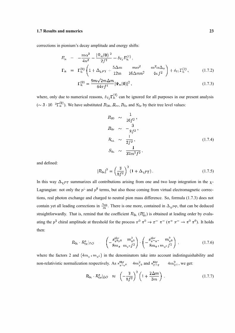
Figure 6: The pionium lifetime as a function of the combination � � �� � � �� � analyzed in the framework of
Generalized � PT. The band delineated by the dotted lines accounts for the uncertainties, coming from theoreticalevaluations, low energy constants and � �� . Values of the lifetime lying below 2.4 fs. remain outside the domain ofpredictions of Standard � PT (large values of � �
� , � 0.28-0.36 correspond to small values of the quark condensateparameter). (Thanks to H. Sazdjian hep-ph/9911520).
��
� �� � �
�� �
�� �
�� � ��
� � ��
�
��
� � � � ��
� ��
�� (1.7.11)
where � ��
� � � and � ��
� � � denote respectively one and two loop contributions in the isospin symmetry
limit ( � = 0, � � = � � = 0) to � � � � and �� � has been chosen at � � , then it is obtained:
� ��
��
� � ��
� � � � �� �
� ��
��
� � (1.7.12)
where the uncertainties are due mostly to the scattering lengths difference. In this 2.9 fs. value enters
roughly a 6% correction to Deser’s formula with a contribution from � � � � � 3.8%.
1.8 Remarks and conclusions
We have presented an approach to pionium’s lifetime calculation which consists of separating
the various dynamical scales involved in the problem by using effective field theory techniques. The
main advantage of this approach is, apart from its simplicity, that error estimates can be carried out
very easily. Before closing this Chapter, a few remarks concerning other approaches are in order.
First of all, relativistic ones[13, 14], besides being technically more involved, have all characteristic
26 Pionium’s lifetime: last stage in a EFT’s chain
physical scales of the problem entangled, which makes very difficult to estimate errors or to gauge the
size of a given diagram. We also would like to emphasize that Lorentz symmetry, even though it is
not linearly realized, it is implemented in our approach to the required order. Several non-relativistic
approaches[15, 27] have appeared in the literature addressing particular aspects of the computation. Our
analysis shows that a coupled channel approach to pionium is unnecessary because � � is much larger
than the bound state energy. It also shows that, although it is technically possible (trivial in fact) to make
a resummation of bubble diagrams a la Lippmann-Schwinger, it does not make much sense since there
are higher derivative terms in the effective Lagrangian, which have been neglected, that would give rise
to contributions of the same order. In a way, our approach implements the already known remark that
neutral pion loops give rise to important contributions in the non-relativistic and supplements it with
relativistic corrections of the same order, which had been overlooked, in a full theoretical framework.
On the technical side we have worked out a new method to calculate the Coulomb propagator�
� ��
��
� � � in DR. The expressions for�
� ��
��
� � � when � � � � are easily obtained for any � . Using
DR here it is not just a matter of taste. Eventually a two loop matching calculation is to be done in order
to extract the parameters of the Chiral Lagrangian from the pionium width. These kind of calculations
are only efficiently done in DR. Since the matching coefficients depend on the renormalization scheme,
it is important to have our calculation in DR in order to be able to use the outcome of such a matching
straight away.
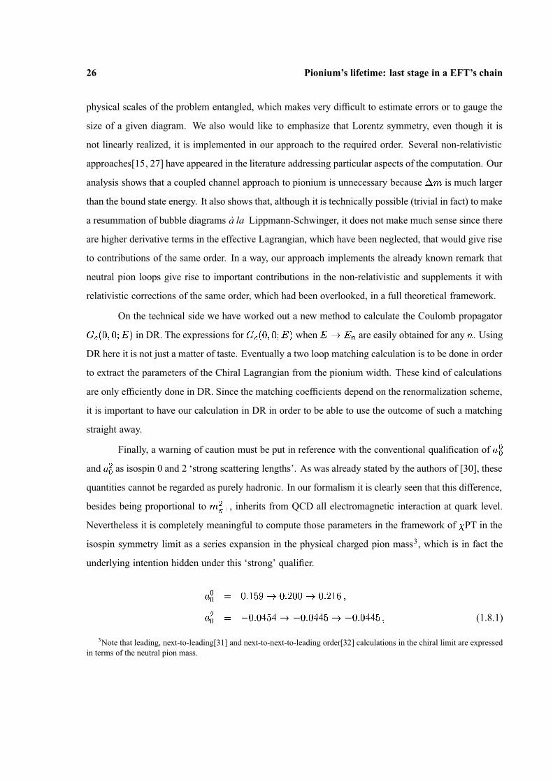
Finally, a warning of caution must be put in reference with the conventional qualification of ���
and ��
� as isospin 0 and 2 ‘strong scattering lengths’. As was already stated by the authors of [30], these
quantities cannot be regarded as purely hadronic. In our formalism it is clearly seen that this difference,
besides being proportional to ��� � , inherits from QCD all electromagnetic interaction at quark level.
Nevertheless it is completely meaningful to compute those parameters in the framework of � PT in the
isospin symmetry limit as a series expansion in the physical charged pion mass3, which is in fact the
underlying intention hidden under this ‘strong’ qualifier.
��� �
��
� � ��
��
� � ��
��
� � �
��
� � ��
��
��
� � ��
��
� ��
� ��
��
� ��
� (1.8.1)
3Note that leading, next-to-leading[31] and next-to-next-to-leading order[32] calculations in the chiral limit are expressedin terms of the neutral pion mass.

1.8 Remarks and conclusions 27
are the numbers so obtained at LO, NLO and NNLO.
Most recent evaluations trust upon different technics in order to pin down their value. Roy
equations, for instance, fully exploit the fact that analyticity, unitarity and crossing symmetry impose
further constraints on the chiral symmetry analysis of the experimental data available at intermediate
energies. The new data from Brookhaven on � � � decays has recently provided the experimental input
that was needed in order to reduce very significantly previous uncertainties (see [33] and figure below).
The scattering lengths may also be extracted from data on pion production off nucleons, as aimed
by the CHAOS collaboration at Triumf, by means of a Chew-Low extrapolation procedure. In this
case, however, chiral symmetry suppresses the one-pion exchange contribution, so that a careful data
selection is required to arrive at a coherent fit.
� ��
� ��
� � � �
� � � �
� � � � �
� � � � �
� � � � �
� � �� � �� � �� � �� � �
Figure 7: Constraints imposed on the � –wave scattering lengths by chiral symmetry. The three full circles illus-trate the convergence of the chiral perturbation series at threshold. The one at the left corresponds to Weinberg’sleading order formulae. The error ellipse represents the 68% confidence contour of the final result of ref. [33].The two dash-dotted lines that touch the ellipse indicate the correlation between �
�� and � �� in this analysis. The
triangle at the right and the shaded rectangle indicate the central values and the uncertainties quoted in the 1979compilation of ref. [34]. The triangle and the diamond near the center of the figure correspond to set I and IIof ref. [35]. Finally, the tilted lines are the universal band, that is the area in the ( �
�� , � �� ) plane allowed by the
constraints given by � � -scattering data above .8 GeV. and the Roy equations.

Chapter 2
Light Fermion Finite Mass Effects in
Non-relativistic Bound States
2.1 Motivation
As, when going from one link to another in the chain of EFTs described in last pages, we
integrated out potential photons a new aspect of our formalism was entering that we wish to develop
further in the present Chapter. The fact is that, whenever two or more physical scales are competing, as
relative momenta and the mass of the electron were then, there is no chance of performing a step-by-
step matching calculation: both must be taken into account at once, no approximations are allowed, and
the matching coefficients’ (potentials in our case) dependences usually lead to somewhat more involved
calculations. At the same time, the EFT framework becomes the only reliable procedure capable of
signaling when a non-perturbative (in � � or �
�
) computation is compulsory. So, in view of the last
calculation, someone might have claimed that for pionium, a system whose reduced mass is something
like 70 MeV., a particle as light as the electron would have made a tiny correction, a negligible one
in any case at the 10% accuracy level. Nevertheless our NREFT calculation relies precisely upon the
existence in a bound state of other energy/momentum scales whose size must also be fixed in respect
with the mass of any light degree of freedom.
The leading effect we are pursuing, -and we will see is not a particularity of the pionium system-
, is a vacuum polarization correction to the energy and to the wave function at the origin, due to light
2.1 Motivation 29
fermions whose mass (from now on � � ) is of the order of the inverse Bohr radius of the Coulomb-
like bound system. This effect, whose importance in the non-relativistic domain of both QED[36] and
QCD[37] is known since long, has attracted lately considerable interest especially in relation with the
� � � system. In fact, for QCD non-relativistic bound states,�
(1S) seems to be, in principle, the only
one amenable to a weak coupling analysis[38]. In nowadays calculations at NNLO of that system,
finite charm mass effects need to be taken into account if we aspire to extract with 1% accuracy the
��
bottom mass from M � . Sharp values of the running heavy quark mass serve us, for instance, to
constrain the allowed parameter space for a given scenario of flavour generation in grand unification
models[39].
Nevertheless, in spite of the fact that one would not say that excited �� � states are Coulombic1,
following [42] one could formally assume we are in the perturbative regime � � � � � � � , calculate
by using NRQCD the quarkonium spectrum and, by comparison with known experimental levels, infer
the size that non-perturbative corrections (together with higher orders in perturbation theory) caused by
local or non-local gluon condensates might have. Perturbative calculations at NNLO including charm
finite size effects show that, surprisingly, within 1-3% accuracy, levels are well reproduced. Although
the net effect of taking into account charm finite mass corrections worsens the agreement by enlarging
splittings, the picture still holds safely due to the uncertainties in �
� �
�� � � � � .
Yet in weak coupling QCD’s domain, we find another important field of application for the
forthcoming displayed corrections in the computation of the total cross section for top quark pair pro-
duction close to threshold in
� annihilation. This cornerstone of the Next Linear Collider’s program
has been recently calculated at NNLL2 with the consequent reduction of the previous NNLO residual
scale uncertainty ( � 20%) down to only 3%. This improvement should lead to an accurate measure
of the top width, the strong top coupling or the top Yukawa coupling in the case of a light Higgs. We
will come back in our Discussion to that issue and will see that finite bottom mass effects in would-be
toponium are right now a sizeable correction worth of being considered to find out the production cross
section for �� � .
1In those relative momenta approaches � � � and it seems more natural to proceed by integrating out both � � and � � � �
at once, as done in [40, 41].2The next-to-next to leading logarithm approximation includes a summation of potentially large logarithms of the scales
� ( 175 GeV.), � � ( 25 GeV.) and � �� ( 4 GeV.), respectively called hard, soft and ultrasoft, by solving the
renormalization group equations for the Wilson coefficients of vNRQCD (velocity NRQCD), as described in [43].Quite recently the N � LO analysis of the heavy-quarkonium spectrum has also been presented [44].

30 Light Fermion Finite Mass Effects in Non-relativistic Bound States
Finally, it is obvious that any QED bound state built out of particles heavier than the electron
may require to take into account its finite mass. Take for instance dimuonium, muonic hydrogen,
pionium, pionic hydrogen and other simple hadronic atoms where �
�
is such that �
�
� � �
� , being �
the bound system’s reduced mass and � its principle quantum number. We discovered in last Chapter the
interest of those atoms, as they carry essential information on the QCD scattering lengths for several
isospin channels, and also found out there that any NLO calculation in � must take into account the
existence of light degrees of freedom, whenever the mentioned condition holds.
That next results can be applied to such a variety of physical systems is a mere by-product
of EFTs. All these non-relativistic bound states have at least three dynamical scales: the mass of
the particles forming the bound state � (hard), its typical relative momentum � � (soft) and binding
energy of order � �� (ultrasoft). Once we integrate the hard scale NREFTs arise. For instance NRQED,
NRQCD and NR � L for QED, QCD and � PT3, respectively. Upon integrating out the soft scale effective
theories which are local in time but non-local in space show up[24, 45]. The non-local terms in space are
the usual quantum-mechanical potentials and only ultrasoft degrees of freedom are left dynamical. The
corresponding non-relativistic effective field theories are named pNRQED, pNRQCD and pNR � L in the
previous cases. Since the leading (mass independent) coupling of the photon field to the non-relativistic
charged particles as well as the one of the gluon field to the non-relativistic quarks is universal, it
produces the same potential in both cases and can be discussed at once. It will be assumed in the
following that we are in the situation in which a light (relativistic) charged particle in QED (or quark in
QCD) whose mass is of the order of the soft scale is also integrated out when going from NR to pNR,
so producing a light fermion mass dependent correction to the static potential.
When matching the NR theories to the pNR theories only the diagram of fig. 1 gives rise to a
potential which contributes as a leading effect. For QED (on-shell scheme) it reads:
� � �� � � � � � � �
��
�� � �
� �
�
� ��
�� �
�
��
� ��
�� � � �
� �� � � � �
� � � � � � (2.1.1)
and for QCD ( � � ):
� � �� � � � � � � �
� � � � � �
�
� �
� � �
� � �
�� �
��
� ��
��
� ��
�� � � �
� �� � � � �
� � � � � ��
�
� � � � ��
�� �� � �� �
3Note the slight departure from the expected NR � PT name, that intends to stress that the calculation in the non-relativisticregime cannot longer be organized according to the chiral counting.

2.2 Energy Shift 31
��
��
��
��
��� �
� � ��
Figure 1: Matching between the non-relativistic theory and the potential one.
� �� � �� �
�� � �
���
� � � ��
� � (2.1.2)
If � � is the number of flavours lighter that � � , the � � � � � above runs with � � � �flavours. Notice
that the difference between the QED and the QCD case is, apart from the trivial colour factors � � � � � �
� � � � � � � � and � � � � � � � � � � , a term which can be absorbed in a redefinition of the Coulomb potential
[46]. Hence for the actual calculation we shall only deal with (2.1.1) and use these facts to extend our
results to the QCD realm.
2.2 Energy Shift
For the energy shift we obtain (� �
� � ��
� � ):
� � � � ��
� � �
��
� �� �
� ��
�� �� �
� � � � ��
� � �� � � � � � � � � � � �
�� �
� � �
� � �
� �
�� � � �
� ��
� � �� � � � � � � � � � � �
�� � � � �
��
��
� ��
� � � � � � ��� � �
���� � � �
�
� � ���� � �
�� � � �
� � � � � � � � � � � � �
� � � � �
� � � � � �� � � � � � � � � �
��
�� � �
� �� � � �
��
� � (2.2.1)

32 Light Fermion Finite Mass Effects in Non-relativistic Bound States
� � ��
��
�
������� �������
� � �� � � � � � � � �
� if�
��
�
�if
��
��
�� � � � �
� � � � � � � � � � ��
� if�
��
�
where � � � � � � ��
��
� is the Coulomb energy. For�
large, namely � � � � � � � � , it reduces to:
� � � � ��
� � � �
��
� �
� �� � � � �
�� � � � � �
� � � � ��
� � ��
� ��
� � ��
� � � ��
�� �
�� � �� �
��
�� �
��
��
� � � ��
��
� ��
� ��
� � � �
��
� � � � ��
� ��
�� �
� �� � � �
� (2.2.2)
whereas for�
small, namely � � � � � � � � , we obtain:
� � � � ��
��
� � �
��
� �� �
� �
��
��
�� � � � �
�� �
��
�� � �
� � � �
�� �
�� �� �
��
� � � � ��
� ��
� � � � � � � � � � � ��
� �� � �
� � �
� �
�� � �
�� �
�� �
�� � � � � � � � � � � �
�� � � �
� � �� �
�
�� (2.2.3)
where we have used (C.4). The key steps to obtain (2.2.1) are given in the Appendix D. We have done
the following checks. For the 1S state (2.2.1) reduces to the result exhibited in Table I (formula (5.3)
of ref. [18]). The energy shifts for the 1S, 2S, 2P, 3S, 3P and 3D states agree with the early analytical
formulas of ref. [47]. For�
large, we reproduce the well-known positronium like limit for � ��
(to
be precise we agree with the correction to the energy obtained using formula (2.8) of [24]). We also
agree for � ��
with formula (32) of ref. [48]. For�
small, we can compare with known results for
massless quarks in QCD. For arbitrary � and � we agree with formula (13) of ref. [46]. For � � � ��
we agree with � �� �
� and � �� �
� of formula (14) in ref. [49]4 but disagree with their � �� �
� result (the
� �� �
� is not displayed in [49]). Notice that for�
large enormous cancellations occur in formula (2.2.1)
and hence the analytic expansion (2.2.2) may prove very useful.
2.3 Wave Function at the Origin
The correction for the wave function at the origin for � ��
states reads:
� � � � � � � � ���
� � � � � �� � �
� ��
��
��
�
� � �� � �
��
��
� ��
� � ��
� � � ��
�
��
4Taking � � � � in that reference and upon correcting an obvious misprint � � � .
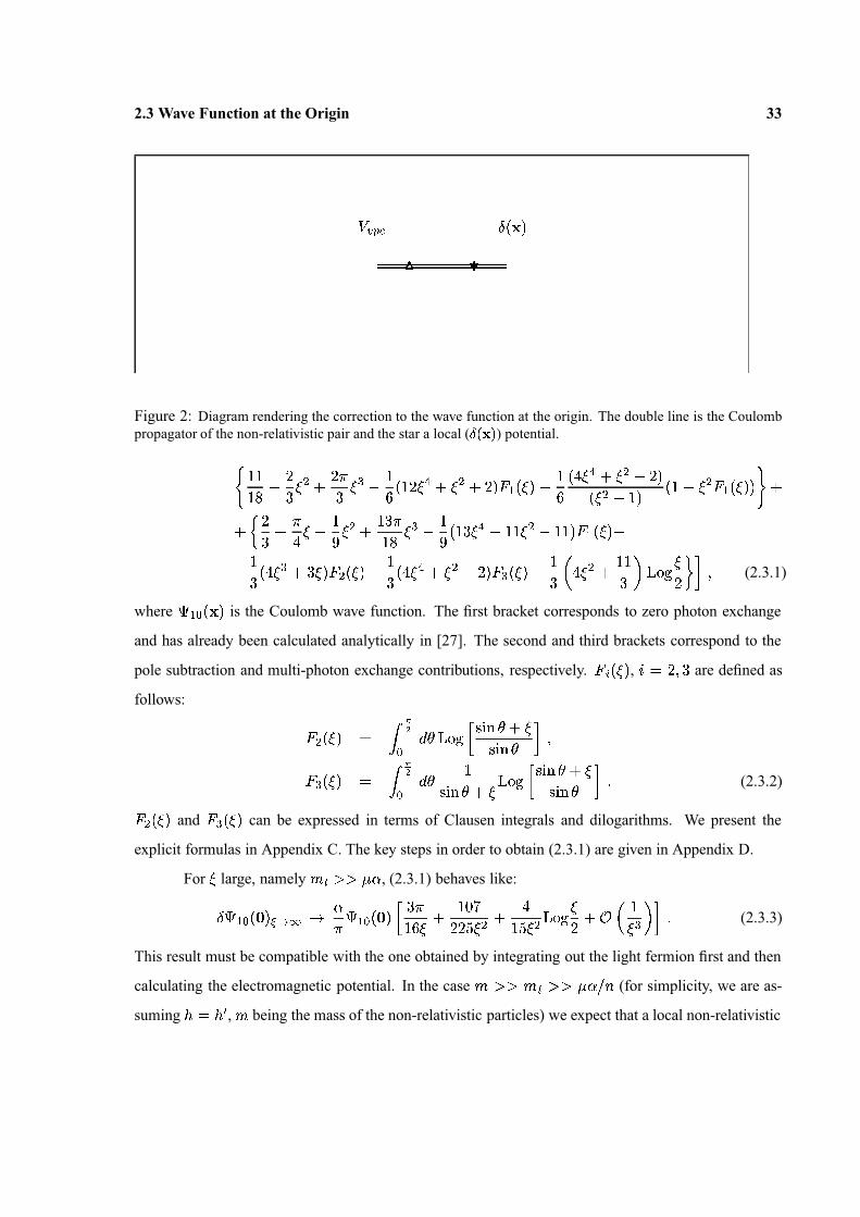
2.3 Wave Function at the Origin 33
� ��
� � � � �
Figure 2: Diagram rendering the correction to the wave function at the origin. The double line is the Coulombpropagator of the non-relativistic pair and the star a local ( � � � � ) potential.
� � �� � �
�
�
� ��
�
�
�
� � ��
� �� � � �
�� �
�
�� � � �
�� �
�� � �
� � �� � �
��
�� � �
��
��
�� �
� � ��
� �� �
�� �
��
�
��
��
� � � ��
� �� �
� � ��
� ��
�� � �
� � � � �� �
� � � ��
� �
��
�� �
� � � ��
� � � ��
� ��
�� �
� � �� � �
�� � � �
�� �
�
�
��
� � �� �
�� � � �
�
�� �
� (2.3.1)
where � � � � � � is the Coulomb wave function. The first bracket corresponds to zero photon exchange
and has already been calculated analytically in [27]. The second and third brackets correspond to the
pole subtraction and multi-photon exchange contributions, respectively. � � ��
� , � ��
� � are defined as
follows:
� � ��
� �� �
��
� � � � � � � � � � ��
� � � � ��
� � ��
� �� �
��
� � �
� � � � �� � � � � � � � � �
�� � � � � � (2.3.2)
� � ��
� and � � ��
� can be expressed in terms of Clausen integrals and dilogarithms. We present the
explicit formulas in Appendix C. The key steps in order to obtain (2.3.1) are given in Appendix D.
For�
large, namely � � � � � � , (2.3.1) behaves like:
� � � � � � � � � � ��
�� � � � � �
� � �� � � �
� � �
� � � � � ��
� � � �� � �
�� � �
� �� � � � � (2.3.3)
This result must be compatible with the one obtained by integrating out the light fermion first and then
calculating the electromagnetic potential. In the case � � � � � � � � � � � (for simplicity, we are as-
suming � � ��, � being the mass of the non-relativistic particles) we expect that a local non-relativistic

34 Light Fermion Finite Mass Effects in Non-relativistic Bound States
��
��
��
��
� ��
Figure 3: Vacuum polarization correction to the decay width at leading order in �� when � � � . Energies andmomenta of order � � and � � � respectively dominate the graph and hence the Coulomb resummation leads tosubleading effects.
effective theory is obtained after integrating out the energy scale � � and the associated three momentum
scale � � � � for the non-relativistic particle. The leading term in (2.3.3) corresponds to the contribu-
tion that would be obtained from the local term induced by the diagram in fig. 3. The logarithm in the
subleading term corresponds to the iteration of two delta function potentials in quantum mechanics (see
formula (1.7.1)). The second delta function is due to the contribution to the electromagnetic potential
of the dimension six photon operator (see [24]) which arises after integrating out a heavy particle[50].
For�
small, namely � � � � � � , we obtain:
� � � � � � � ��
��
� � ��
�� � � � � �
��� �
��
� �� � �
�� �
�� � �� � �
� �� � � (2.3.4)
We have made the following checks. For�
large and small, the leading term of (2.3.3) and (2.3.4) agree
with formulas (22) and (23) of ref. [48], respectively, (the next-to-leading terms are not displayed in
[48]). For�
small we can also compare with known results for massless quarks in QCD. We agree with
the � � � � � correction of formula (69) of ref. [51]. We have also checked that the formula (2.3.1) re-
produces the numerical results obtained for dimuonium and pionium in refs. [52] and [27] respectively,
and we also agree numerically with the analytical result in terms of a non-trivial integral of ref. [48].
2.4 Applications

2.4 Applications 35
2.4.1 Exotic Atoms
We have listed in Table II and Table III the corrections to some energy splittings and to the wave
function at the origin, respectively, of simple exotic atoms of current interest. This purely electromag-
netic corrections must be conveniently taken into account if one wants to obtain precise information of
the strong scattering lengths from hadronic atoms.
�� � �
��
� � �� �� � � � � �
�� � �
��
� � �� �� � � � � �
�� � �
��
� � �� � �
� � � .44593 .38629 -.10453
� � � .18103 .15388 -.056337
� � � .13616 .11548 -.044443
Table II. Vacuum polarization induced energy splittings for some exotic atoms
��
� �
�
�� � � � � � �
� � � �� � � � � �
� � � ��
�
� � � � �� � � �
� � � �� � � �
� � � .21648 .34290 .15454 .09650 .59394
��
� � .28369 .29837 .12958 .08785 .51581
� � � .57635 .19613 .07285 .06166 .33064
��
� � .64357 .18237 .06549 .05741 .30527
� � � .73738 .16627 .05703 .05222 .27552
��
� � 1.00344 .13338 .04052 .04099 .21490
��
� � 1.32550 .10793 .02876 .03184 .16853
Table III. Vacuum polarization correction to the ground state wave function at the origin of some exotic atoms.
2.4.2�
(1S) and �� �
The current calculations of heavy quarks near threshold assume that the remaining lighter quarks
are massless. This approximation is far from being justified at least in two cases. For the�
(1S) system
the typical relative momentum � � � � ��
� 1.3 GeV. [53] is of the same order as the charm mass � � �
1.5 GeV. The effects of a finite charm mass in the binding energy have been quantified in [54]. We
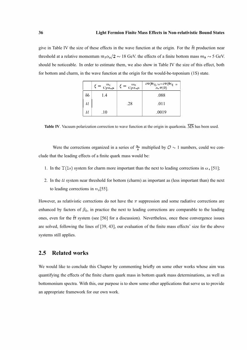
36 Light Fermion Finite Mass Effects in Non-relativistic Bound States
give in Table IV the size of these effects in the wave function at the origin. For the �
� � production near
threshold at a relative momentum ��
� � ��
� 18 GeV. the effects of a finite bottom mass � � � 5 GeV.
should be noticeable. In order to estimate them, we also show in Table IV the size of this effect, both
for bottom and charm, in the wave function at the origin for the would-be-toponium (1S) state.
��
��
� � � �
�
��
� �
� � � �
�
� � � � � � � � �� � � � � � �� �
� � � �
� � � 1.4 .088
�
� � .28 .011
�� � .10 .0019
Table IV. Vacuum polarization correction to wave function at the origin in quarkonia. � � has been used.
Were the corrections organized in a series of� �
� multiplied by � � 1 numbers, could we con-
clude that the leading effects of a finite quark mass would be:
1. In the�
��
� � system for charm more important than the next to leading corrections in � � [51];
2. In the �� � system near threshold for bottom (charm) as important as (less important than) the next
to leading corrections in � � [55].
However, as relativistic corrections do not have the � suppression and some radiative corrections are
enhanced by factors of � � , in practice the next to leading corrections are comparable to the leading
ones, even for the �� � system (see [56] for a discussion). Nevertheless, once these convergence issues
are solved, following the lines of [39, 43], our evaluation of the finite mass effects’ size for the above
systems still applies.
2.5 Related works
We would like to conclude this Chapter by commenting briefly on some other works whose aim was
quantifying the effects of the finite charm quark mass in bottom quark mass determinations, as well as
bottomonium spectra. With this, our purpose is to show some other applications that serve us to provide
an appropriate framework for our own work.

2.5 Related works 37
The determination of the bottom ��
mass is a delicate issue, as illustrated in [39]. In sum rule
analyses at NNLO in the non-relativistic expansion, special care must be taken to eliminate the strong
linear sensitivity to small momenta and its associated (artificially) large perturbative corrections, as well
as large correlations with the choice of the strong coupling constant. This is done by using as expansion
parameter, instead of the bottom quark pole mass, any ‘low-virtuality short-distance’ mass such as the
kinetic mass (Melnikov-Yelkhovsky), the� �
mass (Hoang), the � �mass (Beneke-Singer) or the �
�
mass (Pineda). After this, uncertainties are automatically reduced to a 2% level and further to merely
1% or less just by taking into account some other corrections of straightforward implementation, among
which figures out our charm mass effects.
By formulating observables in terms of a short-distance bottom quark mass, which is expanded
around the light quark massless limit, all IR linear charm mass sensitivity that entered through the
bottom pole mass vanishes, and the first correction to the massless case is of order � � ��
� � � ��� � , which
represents a shift of only a few MeV. and, up to the intended accuracy (tens of MeV.), can be safely
neglected. But the dynamical charm mass effects, filtering through the�
parameter, which is not a small
quantity, represent no negligible corrections as we have just seen. Beware, then, of extractions of the
running bottom mass, which does not show�-dependence and so must remain after being related to a
short-mass parameter, actually affected by�
corrections, that is the one fitted from sum rum analyses
for the masses and electronic decay widths of�
mesons. That is, the leading effect coming from the
finite charm quark mass in the bottom ��
mass as obtained from the bottom� �
mass5 arises at order
� �
� from the fact that one can expand in the charm mass in the bottom pole- ��
mass relation, but not
in the pole-� �
mass one. Schematically:
�� �
� � � � � � � �
� ��
��
� � � � � �� � � � �
�� � � �
� � � � ��
� � � �
� ��
�� � � � � � � � � � � �
� � � � �� �
� � � � �
� ��
�� � � � � � �
��
� � � � �� � � � �
�� � � �
� ��
�� � � � � � � � � � � � �
� � � � �� �
� � � � �
� ��
�� � � � � � � � �
� (2.5.1)
�
� ��
�� � � � �
� ��
�� � � � �� � � �� � �
� � � �� � �
� � � � ��
��
� �� � � � �
�� � � � � � � �
�� �
� � � � �� �
� � � � �� � � �� � � � � � � � ���
�� �
� � � � ��
� � � � � � � ��
� �� � � � �
� �� � � � �� � � �� � � � � � � � �
� (2.5.2)
��
� �� � � � �
� �� � � � �� � � �� � � � � � � �
� ��� � �
�� � � �� � �� (2.5.3)
5The � � mass was first introduced to address the aforementioned problems for bottom and top quark mass extractions from�sum rules and from top-antitop quark pair production close to threshold at NLC. It is defined as half of the perturbative
contribution to the mass of a � �� � � �
, � � � quark-antiquark bound state, assuming that the heavy quark is stable.
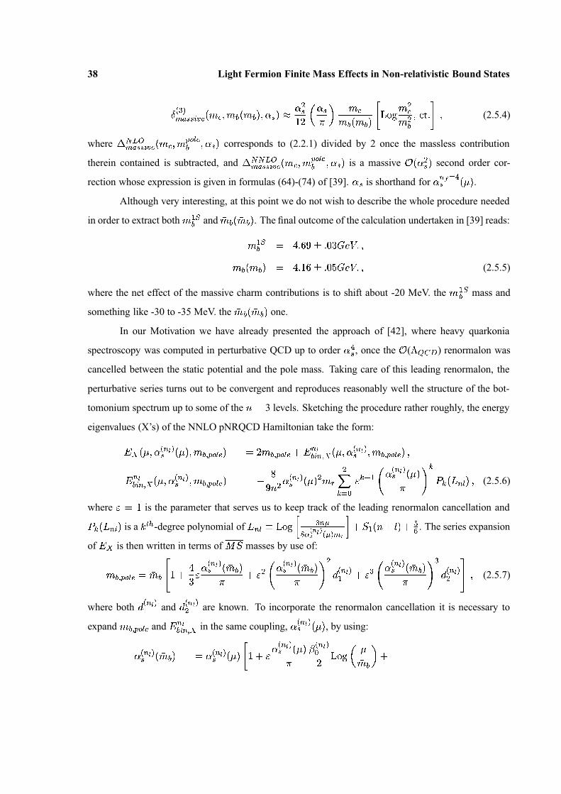
38 Light Fermion Finite Mass Effects in Non-relativistic Bound States
�
�� �
� �� � �
� �� � � �
�
� � ��
� � � � � � � ��
��
� �
�� �
�� � �
�
� � ��
� � �
� � � � ���
�
� �
�
� ��
� � � (2.5.4)
where � � � �� � � � �
� �� � � � �
� ��
�� � � � � corresponds to (2.2.1) divided by 2 once the massless contribution
therein contained is subtracted, and � � � � �� � � � �
� �� � � � �
� ��
�� � � � � is a massive � � � � � � second order cor-
rection whose expression is given in formulas (64)-(74) of [39]. � � is shorthand for �� � � �
� � � � .
Although very interesting, at this point we do not wish to describe the whole procedure needed
in order to extract both �� �
� and�
� � ��
� � � . The final outcome of the calculation undertaken in [39] reads:
�� �
� � � � � � � � ��
��
�� �
�
� � ��
� � � � � � � � � � � � ��
�� � (2.5.5)
where the net effect of the massive charm contributions is to shift about -20 MeV. the �� �
� mass and
something like -30 to -35 MeV. the�
� � ��
� � � one.
In our Motivation we have already presented the approach of [42], where heavy quarkonia
spectroscopy was computed in perturbative QCD up to order � � � , once the � ( � � � ) renormalon was
cancelled between the static potential and the pole mass. Taking care of this leading renormalon, the
perturbative series turns out to be convergent and reproduces reasonably well the structure of the bot-
tomonium spectrum up to some of the � � 3 levels. Sketching the procedure rather roughly, the energy
eigenvalues (X’s) of the NNLO pNRQCD Hamiltonian take the form:
� � � � � �� �
��
� � � � � � � �� �
��
� ��
� � �� �
�� � �
��
� � � � � � � � �� �
��
� � � � �� �
��
� �
��
�� � � � � � � � �
� ��
�� � � � �
� ��
�� � �
�
��
� �� �
��
� � � ��
� ���
� � �� � � � � �
� ��
�� � � �
�� �
� � � � � � � � (2.5.6)
where � ��
is the parameter that serves us to keep track of the leading renormalon cancellation and
� � � � � � � is a � � �-degree polynomial of � � � � � � � � � � � � �
� � � � � � � � �� � � � � �
�� . The series expansion
of � � is then written in terms of ��
masses by use of:
� � �� �
��
��
� �
�� � �
�� �
� ��
�� ��
� � �
�� � � � �
� ��
�� ��
� � �
�� �
�� �
��
� � � � � �� �
��� �
�
� � �
�� �
�� �
��
� �� � (2.5.7)
where both �� �
��
� and �� �
��
� are known. To incorporate the renormalon cancellation it is necessary to
expand � � �� �
��
and ��
�� � � � � in the same coupling, �
� ��
�� � � � , by using:
�� �
��
� ��
� � � � �� �
��
� � � �
�� � � �
� ��
�� � � �
�
�� �
��
� � � � � ��
�
� �
� �

2.5 Related works 39
b
c b
c
a) b)
Figure 4: Feynman graphs responsible for the leading charm mass effects to the pole mass a) and to the Coulombpotential b).
�� � � �
� ��
�� � � �
�� �
� �� �
�� �
�
�
� � � �
��
�
� �
� ��
� ��
��
�� � �
��
�
� �
� � �� � (2.5.8)
So the energy levels take the form:
� � � � � �
� ��
�� � � � �
�
� � � �
��
� � � ��
�
�� �� � � � �
� ��
�� � � � �
�
� � � �� �
��
�� �
� � � � �
��
��
� � � � ��
� � � � ��
� ��
�
�� �
� � � � �
��
��
� � � � ��
� � � � �� � � � � (2.5.9)
form that explicitly realizes the first renormalon cancellation and where, since � � and�
� are short range
quantities, the obtained perturbative expansion is expected to show a better convergence. Until here no
charm mass effects have been taken into account. To do so at first and second order ( � � and � � ), we
consider:
� � � �� � � � � �
� � � �� � �
� � �� � �
� �� � � �
� � ��
� �� � �
� � � � � � � � � �� � � � �
� � �� � �
� �� � � � �
�� �
� � � (2.5.10)
The term � � � �� � �
� � �� � is given in (2.2.1) (b), � � � � �
� � �� � has been calculated in [57] (a), the quantity
� � � �� � �
�� �
� � is only known for� �
bottomonium, and � � � � ��
� �� � has been calculated in the limit � � �
�
(linear contribution) in [39].
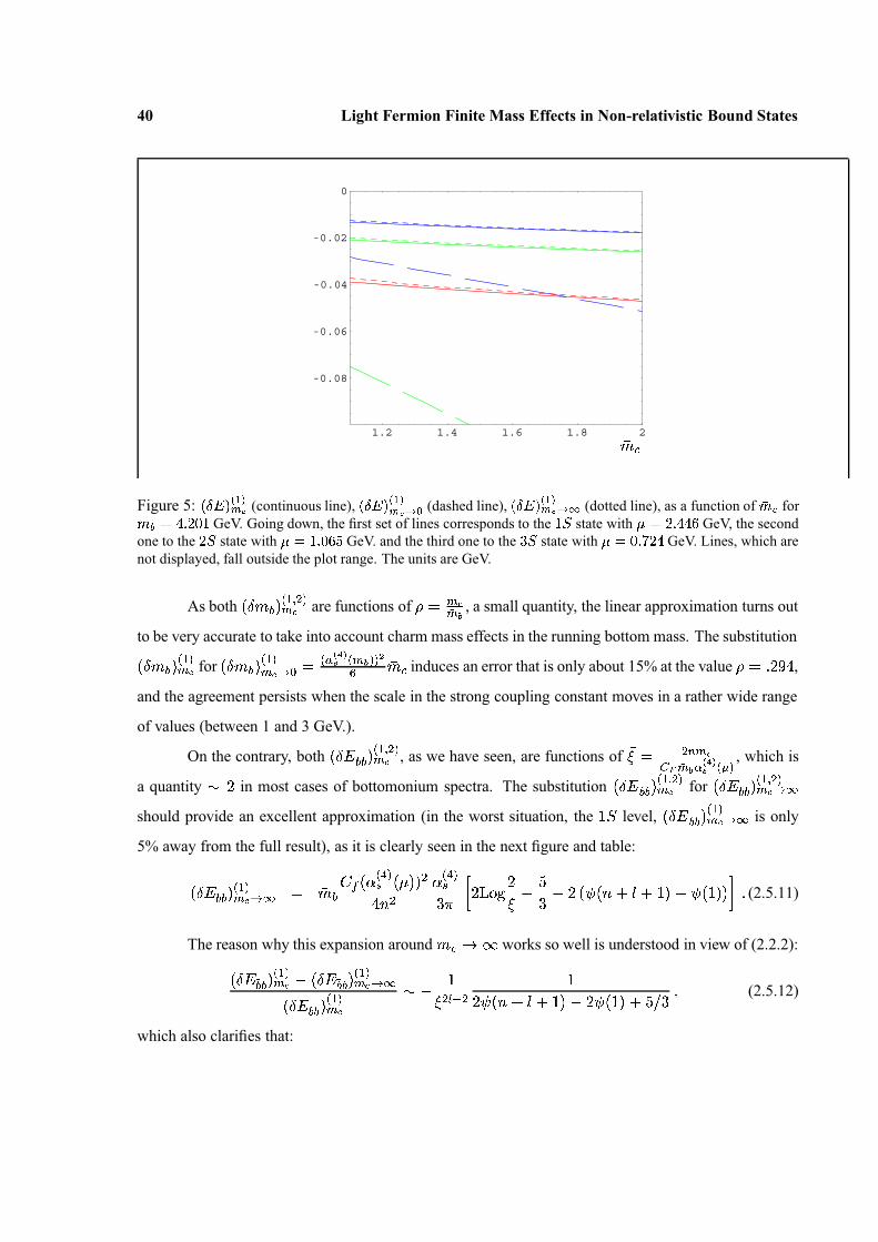
40 Light Fermion Finite Mass Effects in Non-relativistic Bound States
1.2 1.4 1.6 1.8 2
-0.08
-0.06
-0.04
-0.02
0
�
� �
Figure 5: � � � ��
�
�� � (continuous line), � � � �
��
�� � � (dashed line), � � � �
��
�� � � (dotted line), as a function of �� � for
�� � � � ��
� �GeV. Going down, the first set of lines corresponds to the
� state with � � �
� � � �GeV, the second
one to the � state with � � � � � � �GeV. and the third one to the
� state with � � � � � �
�GeV. Lines, which are
not displayed, fall outside the plot range. The units are GeV.
As both � � � � �� � � � ��
� are functions of � ��� �
�� � , a small quantity, the linear approximation turns out
to be very accurate to take into account charm mass effects in the running bottom mass. The substitution
� � � � �� � ��
� for � � � � �� � �
� � � � �� � �
�
�� � �� � � � ��
�
� � induces an error that is only about 15% at the value � � �� � � ,
and the agreement persists when the scale in the strong coupling constant moves in a rather wide range
of values (between 1 and 3 GeV.).
On the contrary, both � � � �� � �
� � � � �� � , as we have seen, are functions of �
�� � � �� �
� � �� � � ��
�� �� � , which is
a quantity ��
in most cases of bottomonium spectra. The substitution � � � �� � �
� � � � �� � for � � � �� � �
� � � � �� � � �
should provide an excellent approximation (in the worst situation, the� �
level, � � � �� � �
� � �� � � � is only
5% away from the full result), as it is clearly seen in the next figure and table:
� � � �� � �
� � �� � � � �
�
� �
� � � �� � �
� � � � ��
� ��
�� � �
�
� �
� � � � �
�
� ��
��
��
�� � � � � �
� ��
��
� �� � (2.5.11)
The reason why this expansion around � � � � works so well is understood in view of (2.2.2):
� � � �� � �
� � �� � � � � � �� � �
� � �� � � �
� � � ��� �
� � �� �� �
�
�
�� � �
�
�� �
� � � � � �� �
� ��
�� � �
� �� (2.5.12)
which also clarifies that:

2.5 Related works 41
State � �
�� �
� � � � �
�� � � �
� � �� � �
� � � � � �� � �
� � �� � � � � � � �
� � �� � �
� � � �
� � �� 2.446 0.277 1.59 � 0.0143 � 0.032 � 0.0136
� � � � 1.140 0.428 2.06 � 0.0210 � 0.076 � 0.0210� � � � 1.111 0.437 2.02 � 0.0221 � 0.079 � 0.0221� � � � 1.086 0.445 1.99 � 0.0232 � 0.082 � 0.0232�
� �� 1.065 0.452 1.96 � 0.0219 � 0.084 � 0.0211�
� � � 0.726 0.695 1.91 � 0.0426 � 0.199 � 0.0424�� � � 0.703 0.733 1.81 � 0.0490 � 0.222 � 0.0488�� � � 0.678 0.782 1.70 � 0.0581 � 0.252 � 0.0579
�� �
� 0.724 0.698 1.90 � 0.0405 � 0.201 � 0.0392
Table V. � � � � � � ��
�
�� � , � � � � � � �
��
�� � � and � � � � � � �
��
�� � � for �� � 4.201 GeV. and �� � 1.237 GeV.; �
��
�� iscalculated from
� ��
��� � � �
� � � GeV. at four loops. All dimensionful quantities are expressed in GeV.
1. states with high � are expected to be reproduced better by the asymptotic approximation;
2. higher � are also, in principle, well reproduced, as�
grows like �� � � �� �
� � and the growing of the
strong coupling constant does not compensate that of � ;
3. charm mass effects can be taken into account in the energy level expansion very effectively by
taking the situation with only three active and massless quarks:
� � � �� � � � �
95%� � � �
� � � � � � � � ��� � � �
� � � � � ��
� �� � � � � � � �
� ��
�� � �
�� � � �� � � � � �
� � �� � � � � � � �
� ��
�� �(2.5.13)
The previous expansions seem to imply that, up to the present level of accuracy, both � � and � � correc-
tions can be safely expanded for small (large)�
� � in the bottom mass (bottomonium binding energy),
so resulting in:
� �� � �
���
� �
�� � � � ��
� �� � �
� � � � �
�� � � � �
� � �� � � � �
�� �
�� � �� � � � � �
� � �� � � � �
�� �
�� � �
�� �� �
� ��� � � �
� �
��� � �
�� �
� � � � � � �
�� � � � ��
� �� � �
� � � � �
�� � � � �
� � �� � � � �
�� �
�� � �� � �� �
��� � �
�� � � � �
� � �� � � � �
�� � �� � � � �
�� �
� � ��
� � � � �� � �
� � � �
�
� �
� � � � �� � �
� �� �� �� � � � ��
� � � Eq. (2.5.8)� � � ��
� Eq. (2.5.15)� �� � � �
� � ��� � � � � �
�� �
� � � � ��
� � � � � � � � ��
� ��� � � � � �
�� �
� � � � ��
� � � � � � � �
� ��
� ��� � � � �
�� �
� � � � ��
� � � � � � � � � � � � � (2.5.14)
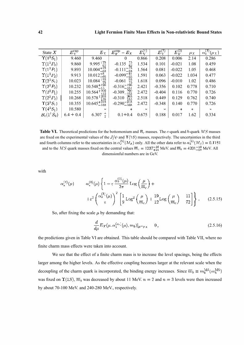
42 Light Fermion Finite Mass Effects in Non-relativistic Bound States
State � � � � �� � � � � � �� � � � �� � �
� ��
� �� �
�� �
� � � ��
� �� � � � �
��
� � �� � 9.460 9.460 0 0.866 0.208 0.006 2.14 0.286
��
� � � � � 9.860 9.995� � �
��
� -0.135 �� �
� �� 1.534 0.101 -0.021 1.08 0.459
��
� � � � � 9.893 10.004� � �
��
� -0.111 �� �
� �� 1.564 0.081 -0.022 1.05 0.468
��
� � � � � 9.913 10.012� � �
��
�
-0.099 �� �� �
�
1.591 0.063 -0.022 1.034 0.477�
��
� �� � 10.023 10.084
� ��
�� �
-0.061 ��
�� � �
1.618 0.096 -0.010 1.02 0.486�
��
� � � � 10.232 10.548� � � �
� ��
� -0.316 � � � �
� ��
� 2.421 -0.356 0.102 0.778 0.710�
��
� � � � 10.255 10.564�
� � �
� ��
� -0.309 � � � �� ��
� 2.472 -0.404 0.116 0.770 0.726�
��
� � � � 10.268 10.578�
� � �
� �� �
-0.310 � � � �� �� �
2.518 � 0.449 0.129 0.762 0.740�
� � � �� � 10.355 10.645
�� � �
� � � � -0.290 � � � �� � � � 2.472 -0.348 0.140 0.770 0.726
�� �
� �� � 10.580 � � � � � � �� � �
� � �� � 6.4
�0.4 6.307
� �� � 0.1
�0.4 0.675 0.188 0.017 1.62 0.334
Table VI. Theoretical predictions for the bottomonium and � � masses. The � -quark and � -quark � � massesare fixed on the experimental values of the � � and � �
�� � masses, respectively. The uncertainties in the third
and fourth columns refer to the uncertainties in �
� �� � � � � only. All the other data refer to �
� �� � � � � �
� � � ��
�
and to the � � quark masses fixed on the central values � � ��
� � � � �� � � MeV. and � � �
�
� � � � �� � � MeV. Alldimensionful numbers are in GeV.
with
�� � �
� � � � � ��
� �� � � �
��
�� �
�� �� � � �
� �
� � ��
�� � � �
�� � � �
�� �� � � �
�� � � �
�� � � �
��
� � � �
� �� � � � �
��
� � � �� �
� � � � �� � (2.5.15)
So, after fixing the scale � by demanding that:
�� �
� � � � � �� � � �
� � � � � �� � � ��
�� � �
�� (2.5.16)
the predictions given in Table VI are obtained. This table should be compared with Table VII, where no
finite charm mass effects were taken into account.
We see that the effect of a finite charm mass is to increase the level spacings, being the effects
larger among the higher levels. As the effective coupling becomes larger at the relevant scale when the
decoupling of the charm quark is incorporated, the binding energy increases. Since � � � � � �� � � � �� �
was fixed on�
�� �
� , � � was decreased by about 11 MeV. � ��
and � � � levels were then increased
by about 70-100 MeV. and 240-280 MeV., respectively.

2.5 Related works 43
State � �
��
�� � � �
��
�� � � � �
� � �� �
�� �
� ��
� �� � � � � � � � ��
��
3.097 3.097 0 0.362 0.205 0.043 1.07 0.448� � �
� � �� � 2.980 3.056 -0.076 0.333 0.195 0.042 1.23 0.399
��
� � �� � 9.460 9.460 0 0.837 0.204 0.013 2.49 0.274
��
� � � � � 9.860 9.905 -0.045 1.38 0.115 0.003 1.18 0.409�
�� � � � � 9.893 9.904 -0.011 1.40 0.098 0.002 1.15 0.416
��
� � � � � 9.913 9.916 -0.003 1.42 0.086 0.003 1.13 0.422�
��
� �� � 10.023 9.966 +0.057 1.46 0.093 0.009 1.09 0.433
��
�� � � � 10.232 10.268 -0.036 2.37 -0.66 0.15 0.693 0.691
��
�� � � � 10.255 10.316 � -0.061 � 3.97 -3.56 1.50 0.552 � 1.20
��
�� � � � 10.268 10.457 � -0.189 � 4.55 -5.03 2.53 0.537 � 1.39
�� � � �
� � 10.355 10.327 +0.028 2.34 -0.583 0.163 0.698 0.684�
� � � �� � 10.580 11.760 � -1.180 � 5.45 -6.47 4.38 0.527 � 1.61� � �
� � �� � 6.4
�0.4 6.324 0.08
�0.4 0.668 0.187 0.022 1.64 0.329
Table VII. Comparisons of the theoretical predictions of perturbative QCD and the experimental data. � � �
�
for � � � systems and � � �
�for �� � and �� � systems. All dimensionful numbers are in GeV. units.
As the uncertainties originating from the error of the input �� �
�� � � � � are as large (even larger)
than other uncertainties, both unknown high-order corrections and next-to-leading order renormalons
are expected to contribute some�
��– �
�� MeV. in the case of
� �,
��
� �–
��
�� MeV. for � �
�
states
and about�
� � �–
� � �� MeV. in � � � ones.
Chapter 3
Renormalization issues in
Nucleon-Nucleon EFT
3.1 Motivation
Until the moment we have discussed different applications of non-relativistic EFT’s well-grounded
corpus. Let us now deviate our attention to not so solid terrain. Non-perturbative renormalization, as it
is required to treat nucleon-nucleon (NN) interaction, remains a controversial issue, mainly due to our
partial lack of understanding of the underlying dynamics and, as a consequence, our inability to consis-
tently organize the EFT calculation. That is why our first approach to the subject is going to focus on
power counting and the binomial iterated versus perturbative interactions. We consider that, from that
viewpoint, the renormalization problem is presented in the right perspective and its inherent complexity
is gazed at in all its depth.
Weinberg’s original suggestion[58] that NN scattering and nuclear physics problems could fruit-
fully benefit from a EFT approach was followed by a huge amount of work undertaken, not to improve
the fits of the already successful semi-phenomenological models (Paris, Bonn or Nijmegen potentials),
but to provide a better understanding of the relationships among related processes and the underlying
physics. NN EFTs were expected to disentangle the various physical scales therein involved: � , the
nucleon mass, vector and scalar meson masses as � � and � � and some nucleon resonances’ splittings
were tagged as large ( � 1 GeV); whereas Goldstone boson (GB) masses, � � basically, and the splitting

3.1 Motivation 45
�� - � were categorized as the low energy, dynamical part of the spectrum ( � 200 MeV). Further-
more, NN EFTs were expected to correctly implement the constraints derived from chiral symmetry in
the nucleon-pion interaction. This program, invaluable for reproducing low-energy characteristics of
NN scattering, has found in the non-perturbative nature of nuclear forces its most serious difficulty to
prosper.
Consider in first place what happens in a long-tradition EFT such as � PT, which is perturbatively
renormalizable (in a EFT sense). There, we can truncate the expansion of any observable quantity and
assign an error estimate to its amplitude just by declaring which is next order in the perturbative series
(say, for instance, � � � � ��
�� if we wish a � � � accuracy in our calculation). By performing some power
counting on diagrams, –remember that whenever we have � loops,�
� vertices of type � which contain
� � derivatives and � � fermion fields, our graph is order � � ,
��
�� � � �
� ��
�
�� � � � � � � � � � � �� �
�� (3.1.1)
– we learn up to which order our Lagrangian is required. That is, we would need the set of interactions
�� �
� , � ��
� � � � ��
� ��
where �
� �, in the previous case. As our Lagrangian is an expansion
in powers of momenta, loops are going to be increasingly divergent as we keep including higher order
vertices. Nevertheless they can be regulated (let us refer to a cutoff � for convenience, although dimen-
sional regularization is the optimal way to work at in this context) and the severe cutoff dependence
coming from the high momenta region, which otherwise is not correctly described by the EFT, can be
removed by lumping these terms together with the unknown bare parameters � �
� �� � into renormal-
ized coefficients � �
�
�
� � . As you see, for the most divergent dependence we have at our disposal the
brand-new group of vertices � � � � � � �� � . Those ensure renormalization scale independence at every
order in the EFT expansion of observables.
Unfortunate complications arise whenever we face in a EFT with the presence of shallow bound
(quasi-bound) states. As, to generate them, some interactions must be resummed using a Schr �� dinger
or Lippmann-Schwinger equation, first of all, one should try to work out some criteria that allow us
to decide which terms are leading order and, therefore, must be iterated, and which ones are mere
perturbations. Accordingly, contact interactions would be ordered in ever growing powers of the inverse
cutoff. Large scattering lengths in NN interactions require, indeed, some of the latter to be tagged
as leading order potentials, with the consequent appearance of more acute divergences as we keep

46 Renormalization issues in Nucleon-Nucleon EFT
increasing the order of the iteration. That is the point where the regularization and non-perturbative
renormalization issues enter.
As we notice, so proceeding, any justification on the power counting is made a posteriori, once
we compute our phase shifts or any other observables and verify that they are reasonably well repro-
duced (up to the intended accuracy), while cutoff dependence is being removed in this order-by-order
expansion of the amplitude. To provide for a solid, consistent renormalization program of NN interac-
tions has become, as it is shown in the next section, a most debated object and, at the same time, a most
desirable one if one is interested in lending EFT’s sound techniques to nuclear calculations. Only after
we have attained a fair comprehension of the hierarchies involved and low-energy constants fine-tuning,
will be able to relate different NN low-energy processes model-independently.
So, before going on, it would be most interesting to review briefly what is the status of matter
reached after several studies which tested various regularization schemes, power countings and more
or less rigorous approaches. Nevertheless, in view of the huge amount of bibliography this question
has generated, regretfully we better opt to focus only on three or four recent works chosen, not only
in regard to their intrinsic value, but also because we consider they are useful in providing a way of
comparison with our own work.
3.1.1 Reporting on previous work
Although our final purpose is to consider NN interactions as mediated by exchanged pions plus local
sources of short-distance repulsion, in order to have a nodding acquaintance with the complexity of
the problem, let us consider first, following refs. [59] a simplified EFT for NN interaction in the � ��
channel, a theory in which all exchanged particles have been integrated out:�
� ��
� � � � � � � � � ��
� �� �
� � (3.1.1.2)
This should deliver a reasonable description of the NN scattering amplitude at low-energy (� , ��
�
� � ), as
�
� � � �
�
� � ��
� � ��
� ��
��
� ��
� � � � � (3.1.1.3)
is the effective range expansion. Nevertheless, our first surprise comes when we realize that although
these�
� coefficients are naively expected to scale as ��
�� �
�� �
� , they are fixed by a rather lower scale,

3.1 Motivation 47
on the order of � �
� �MeV. Such a behaviour is associated to this channel’s large scattering length:
�
�
� ���
� ��
� � � � � � � ��
� ���
��
� � � � � � (3.1.1.4)
or, what comes to be equivalent, to its low lying nearly-bound state. In fact also the spin triplet channel
suffers from the same particularity, with the difference that what is found now is a real bound state:
�� � �
�� � �
� � � � �� � �
�� � � � � � � (3.1.1.5)
But perhaps, following Weinberg’s suggestion, one may expect that making an EFT expansion of the
potential and iterating it through a Lippmann-Schwinger equation one could still generate these loosely
bound states, while maintaining natural coefficients in the potential:
�
� � � ��
� � � ��
� � � ��
� �� � �
�� �
��
� � �
�� � � �
� ��
�
� �
�� � �� � � �
� � �� �
� ��
� � � � (3.1.1.6)
After inserting (3.1.1.2) above it is evident that what we are doing in fact is generating new difficulties.
That is, severe divergences arise and demand a sensible procedure to regularize and renormalize them
non-perturbatively, so conditioning the existence of the EFT. To be concrete, our solution of the T-
matrix:�
�
� � ��
� � � � � ��
��
� � � �� �
�� � � � � �
�� � � � � �
� � � � (3.1.1.7)
��
� � �
� � ��
� ��
�� � � �
� � �� � � � � �
� � ��
� ��
�� � � � � � � �
� � ��
� ��
�� � �
�
� � � �� � � � � �
�
where � is the on-shell momentum, contains the power-law divergent integrals ��, � � and � � , that can
be regularized either using a cutoff (sharp or smooth), by dimensional regularization with minimal
subtraction ( � � � � ) or any other appropriated choice. In � � � � the divergent pieces of every integral
vanish by prescription and it is straightforward to match both coefficients � and � � to the experimental
scattering length and effective range by means of the effective range expansion:�
�� � �
� ��
� �
��
�
��
�� �
� � � � � � �� � � � � � (3.1.1.8)
so yielding:�
� � �� � �
� ��
� �� �
�
� � ��
� �� �
� �� � � � �
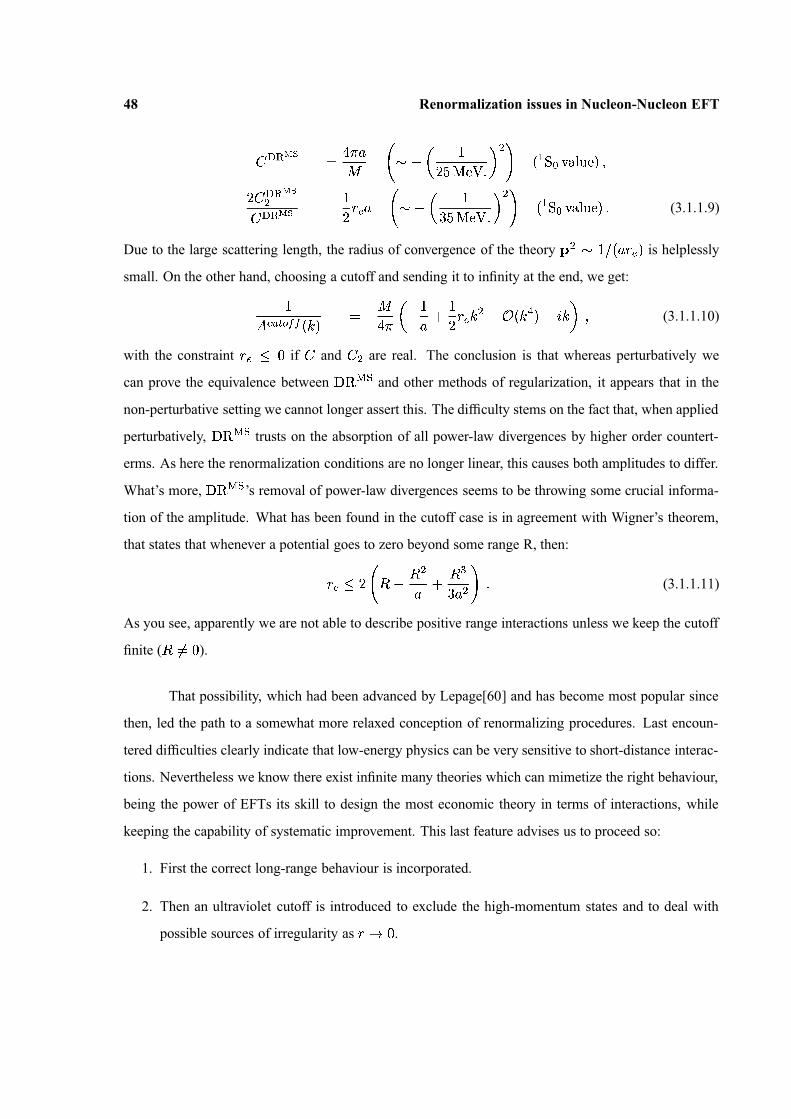
48 Renormalization issues in Nucleon-Nucleon EFT
�� � � �
�
� � �
�� � �
� �� �
� � � � � � � ��
� � ��
� �� � �
�
�� � � �
�
�� � � � �
�� �
�� � � �
� �
��
� � � � � � � ��
� � ��
� �� � � (3.1.1.9)
Due to the large scattering length, the radius of convergence of the theory ��
�
� � � � ��
� is helplessly
small. On the other hand, choosing a cutoff and sending it to infinity at the end, we get:�
� � � �� � �
� � �� �
�
� �
��
�
��
�� �
� � � � � � � �� � � � � � (3.1.1.10)
with the constraint �� �
if � and � � are real. The conclusion is that whereas perturbatively we
can prove the equivalence between � � � � and other methods of regularization, it appears that in the
non-perturbative setting we cannot longer assert this. The difficulty stems on the fact that, when applied
perturbatively, � � � � trusts on the absorption of all power-law divergences by higher order countert-
erms. As here the renormalization conditions are no longer linear, this causes both amplitudes to differ.
What’s more, � � � � ’s removal of power-law divergences seems to be throwing some crucial informa-
tion of the amplitude. What has been found in the cutoff case is in agreement with Wigner’s theorem,
that states that whenever a potential goes to zero beyond some range R, then:
�� � � � � � �
�� � �
� ��
� � (3.1.1.11)
As you see, apparently we are not able to describe positive range interactions unless we keep the cutoff
finite ( � �� �).
That possibility, which had been advanced by Lepage[60] and has become most popular since
then, led the path to a somewhat more relaxed conception of renormalizing procedures. Last encoun-
tered difficulties clearly indicate that low-energy physics can be very sensitive to short-distance interac-
tions. Nevertheless we know there exist infinite many theories which can mimetize the right behaviour,
being the power of EFTs its skill to design the most economic theory in terms of interactions, while
keeping the capability of systematic improvement. This last feature advises us to proceed so:
1. First the correct long-range behaviour is incorporated.
2. Then an ultraviolet cutoff is introduced to exclude the high-momentum states and to deal with
possible sources of irregularity as � � �.
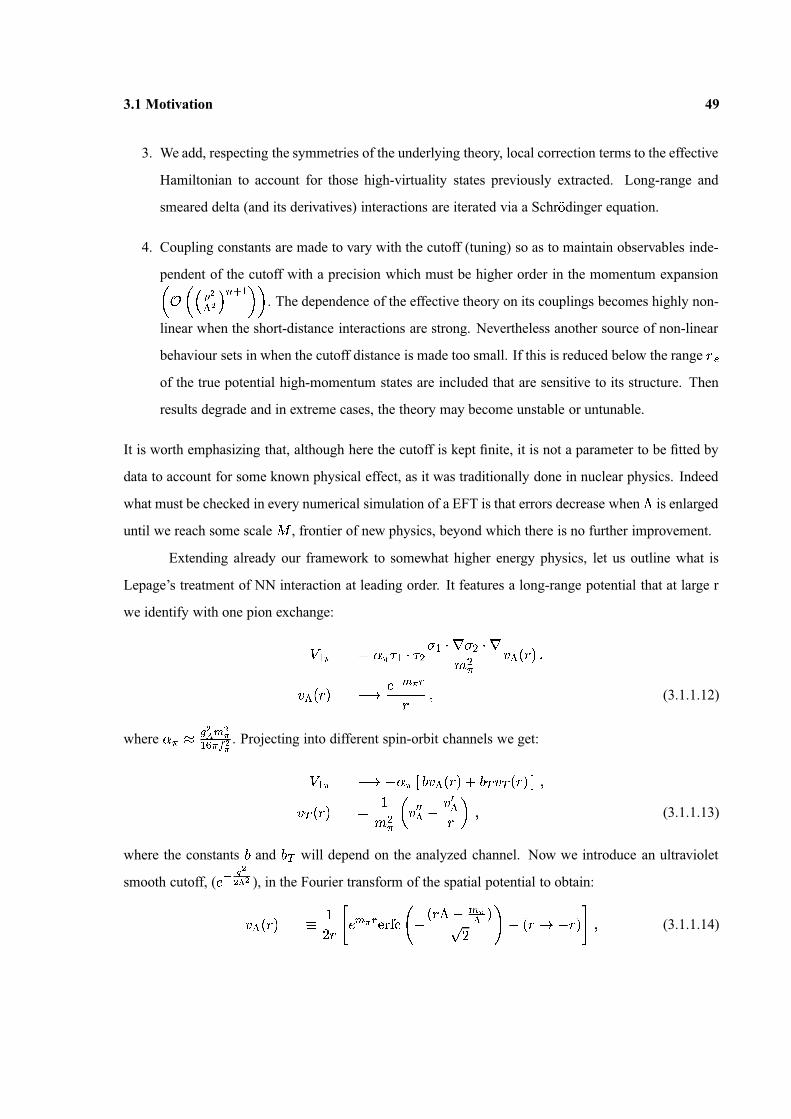
3.1 Motivation 49
3. We add, respecting the symmetries of the underlying theory, local correction terms to the effective
Hamiltonian to account for those high-virtuality states previously extracted. Long-range and
smeared delta (and its derivatives) interactions are iterated via a Schr �� dinger equation.
4. Coupling constants are made to vary with the cutoff (tuning) so as to maintain observables inde-
pendent of the cutoff with a precision which must be higher order in the momentum expansion��
� � � �� � � �
� � � � . The dependence of the effective theory on its couplings becomes highly non-
linear when the short-distance interactions are strong. Nevertheless another source of non-linear
behaviour sets in when the cutoff distance is made too small. If this is reduced below the range ��
of the true potential high-momentum states are included that are sensitive to its structure. Then
results degrade and in extreme cases, the theory may become unstable or untunable.
It is worth emphasizing that, although here the cutoff is kept finite, it is not a parameter to be fitted by
data to account for some known physical effect, as it was traditionally done in nuclear physics. Indeed
what must be checked in every numerical simulation of a EFT is that errors decrease when � is enlarged
until we reach some scale � , frontier of new physics, beyond which there is no further improvement.
Extending already our framework to somewhat higher energy physics, let us outline what is
Lepage’s treatment of NN interaction at leading order. It features a long-range potential that at large r
we identify with one pion exchange:
�� � � � � � � �
��
� � �� �
� ��
� �� � � � � � �
� � � � � � �� �
� � �
�� (3.1.1.12)
where � � �� �� � ��
� � � � �� . Projecting into different spin-orbit channels we get:
�� � � � � � � � � � � � � � � � � � � � � � � �
� � � � � ��
� ���
�� �� �
���
�� � (3.1.1.13)
where the constants � and � � will depend on the analyzed channel. Now we introduce an ultraviolet
smooth cutoff, ( � �� �
� � � ), in the Fourier transform of the spatial potential to obtain:
� � � � � �
��
�
��
� � ��
��
� � �� � � �
� �� �
�� � � � � � � � � � � (3.1.1.14)

50 Renormalization issues in Nucleon-Nucleon EFT
� ��
�
� ��
�
� ��
�
�
� � � � � � � � �
� � � � � � � �
� � � ��
�
� �
� �� �
�
� � �� �
�
� ��
� ��
�� �
� ��
Figure 1: Errors in the � � � phase shifts (in radians) versus energy for the full effective theory with differentvalues of the cutoff
�.
and the function erfc(x) stands for 1-erf(x) (error function). The short distance terms in the potential
are smeared delta functions (and its derivatives):
�
�� �
� � � � � � �
��
� �
� � � ��
��
� �� �
� (3.1.1.15)
In all, nine constants account for two S and four P waves up to order � � ��
� .
Take � �� channel at this accuracy. It requires the tuning of two short distance couplings to, let’s
say, the phase shifts at two different energies. Our potential is:
�� � � � � � � �
� � � � � ��
�� �
� � � � � �
� � � � � ��
�� �
� � � � � �
� � � (3.1.1.16)
The errors obtained in the phase shift as a function of the center of mass energy are found in fig. 1.
Errors decrease until � � 300 MeV. and afterwards no further improvement is seen. The low radius
of convergence of the theory can perhaps be explained by two-pion exchange role, isospin breaking
effects, � (the baryonic resonance with I=3/2) contributions or some tuning of � � .
So, should we content with this new viewpoint or should we pursue in trying to find out a more
conventional renormalization program -a program where one merely regulates the integrals and then
renormalizes the couplings of the theory so absorbing all terms that diverge as the cutoff is removed?

3.1 Motivation 51
� ��
�
� ��
�
� ��
�
�
� � � � � � � � �
� � � � � � � �
� � � ��
�
�
� �
� �
�
� �
�
Figure 2: Errors in the � � � phase shifts (in radians) versus energy for the effective theory through orders�
� �and
�� � . Results from the theory with just pion exchange ( � � � ) are also shown. The cutoff was
��
� � �MeV in
each case.
Firstly, we want to review DR’s treatment of NN interaction to see where lies exactly the problem and
whether there is any possibility of circumventing it. Let’s borrow for a while that opinion (page 34 in
[61]) which states that constraint (3.1.1.11) although ‘unusual it is doubtful of much relevance to EFTs
applied consistently to a certain order’, as it is ‘a regularization-scheme-dependent issue’.
So take once more � �� channel in the pionless theory and remember what we did in order to
get DR’s result: we expanded the potential up to order ��
(terms of � ��
� and iterated it through
a Schr �� dinger/LS equation. Now we want to do something quite different. After Kaplan, Savage and
Wise suggestion (KSW, [63]), we will expand the inverse of Feynman’s amplitude. This is shown
diagrammatically in fig. 3.
�� �
��
�
��
�
� ��
��
� �
� ��
��
� � � � �� �
��
��
� ��
� � � � � � � (3.1.1.17)
�� and
�� are found to be:
�� � �
�� � � � � � � �
� ��
� ��
�
�� � � � � �
�� � � �
� � � � � � � �� �
� � � �� � �
�
� �� �
��
��
� �� �
� ��
��
� (3.1.1.18)
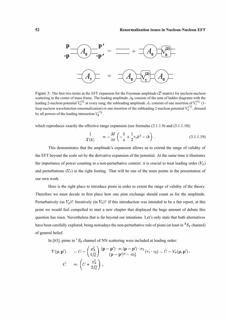
52 Renormalization issues in Nucleon-Nucleon EFT
+=-p’
p’A0-p
pA0
(2)V0
=A1 0A A0(2)
V1
Figure 3: The first two terms in the EFT expansion for the Feynman amplitude ( � -matrix) for nucleon-nucleonscattering in the center of mass frame. The leading amplitude � � consists of the sum of ladder diagrams with theleading 2-nucleon potential �
�
��
� at every rung; the subleading amplitude ��
consists of one insertion of �
�
�
�
�
(1-loop nucleon wavefunction renormalization) or one insertion of the subleading 2-nucleon potential �
�
��
�
, dressedby all powers of the leading interaction �
�
��
� .
which reproduces exactly the effective range expansion (see formulas (3.1.1.9) and (3.1.1.10):�
� � � �� �
�
� �
��
�
�
��
� �� � �
� � � � � (3.1.1.19)
This demonstrates that the amplitude’s expansion allows us to extend the range of validity of
the EFT beyond the scale set by the derivative expansion of the potential. At the same time it illustrates
the importance of power counting in a non-perturbative context: it is crucial to treat leading order (�
� )
and perturbations (�
� ) in the right footing. That will be one of the main points in the presentation of
our own work.
Here is the right place to introduce pions in order to extent the range of validity of the theory.
Therefore we must decide in first place how one pion exchange should count as for the amplitude.
Perturbatively (as�
� )? Iteratively (in�
� )? If this introduction was intended to be a fair report, at this
point we would feel compelled to start a new chapter that displayed the huge amount of debate this
question has risen. Nevertheless that is far beyond our intentions. Let’s only state that both alternatives
have been carefully explored, being nowadays the non-perturbative role of pions (at least in � �� channel)
of general belief.
In [63], pions in � �� channel of NN scattering were included at leading order:
�
� � � ��
� � � � � �� � ��
� � � � ��
� �
� � � � � ��
� �
��
� � � ��
� � � � ��� � � �
�� � �
� �
�� � � � �
�� �
� �
� � �� ��
� ��� �
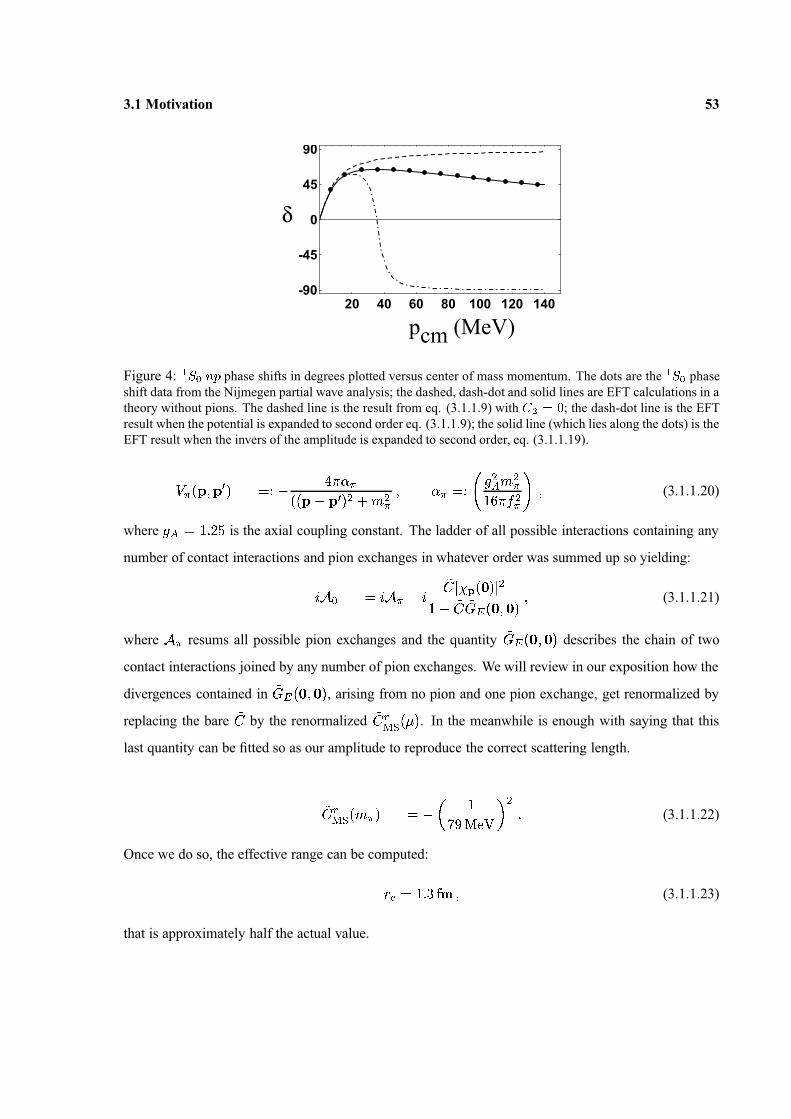
3.1 Motivation 53
δ
pcm (MeV)20 40 60 80 100 120 140
-90
-45
0
45
90
Figure 4: � � � � � phase shifts in degrees plotted versus center of mass momentum. The dots are the � � � phaseshift data from the Nijmegen partial wave analysis; the dashed, dash-dot and solid lines are EFT calculations in atheory without pions. The dashed line is the result from eq. (3.1.1.9) with �
��
�; the dash-dot line is the EFT
result when the potential is expanded to second order eq. (3.1.1.9); the solid line (which lies along the dots) is theEFT result when the invers of the amplitude is expanded to second order, eq. (3.1.1.19).
�
� � � � ��
� �
��
� � � �
� � � � ��
� � � � ��
� � � �� � � �� �
��
� �� � ��
� � (3.1.1.20)
where � � �� �
� �is the axial coupling constant. The ladder of all possible interactions containing any
number of contact interactions and pion exchanges in whatever order was summed up so yielding:
� �� � � � � � �
�
� � � � � ��
��
�
��
� � � � � �� (3.1.1.21)
where� � resums all possible pion exchanges and the quantity
��� � � � � � describes the chain of two
contact interactions joined by any number of pion exchanges. We will review in our exposition how the
divergences contained in��
� � � � � � , arising from no pion and one pion exchange, get renormalized by
replacing the bare�
by the renormalized�
�
�� �
� � � . In the meanwhile is enough with saying that this
last quantity can be fitted so as our amplitude to reproduce the correct scattering length.
�
�
�� �
� � � � � �� �
� �� � �
� �
� (3.1.1.22)
Once we do so, the effective range can be computed:
�
�� � �
� � � (3.1.1.23)
that is approximately half the actual value.
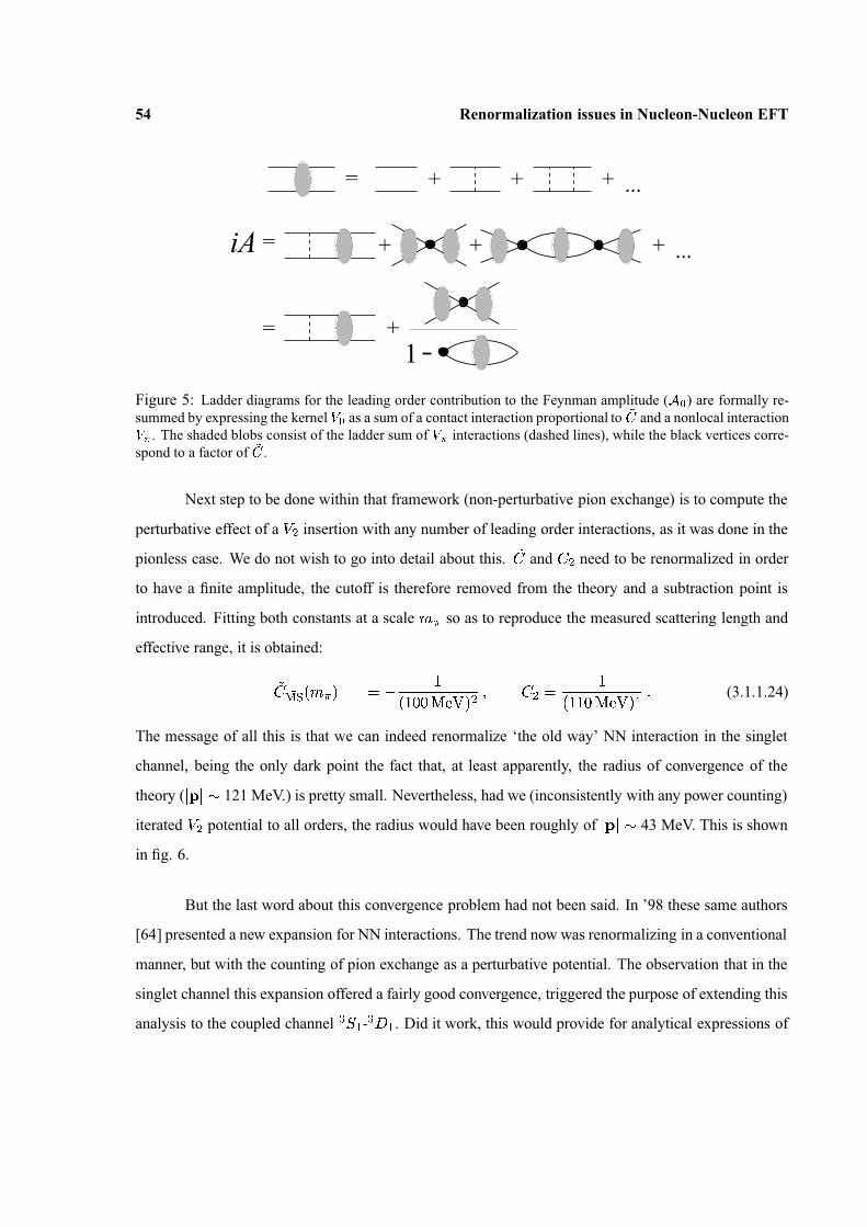
54 Renormalization issues in Nucleon-Nucleon EFT
= + + ...+
+=1
=iA ++ + ...
Figure 5: Ladder diagrams for the leading order contribution to the Feynman amplitude ( � � ) are formally re-summed by expressing the kernel � � as a sum of a contact interaction proportional to �� and a nonlocal interaction
��
. The shaded blobs consist of the ladder sum of ��
interactions (dashed lines), while the black vertices corre-spond to a factor of �� .
Next step to be done within that framework (non-perturbative pion exchange) is to compute the
perturbative effect of a�
� insertion with any number of leading order interactions, as it was done in the
pionless case. We do not wish to go into detail about this.�
� and � � need to be renormalized in order
to have a finite amplitude, the cutoff is therefore removed from the theory and a subtraction point is
introduced. Fitting both constants at a scale � � so as to reproduce the measured scattering length and
effective range, it is obtained:
�� �
� �� � � � � �
�
�� � �
� � � � � � � � �
�
�� � �
� � � � � � (3.1.1.24)
The message of all this is that we can indeed renormalize ‘the old way’ NN interaction in the singlet
channel, being the only dark point the fact that, at least apparently, the radius of convergence of the
theory ( � � � � 121 MeV.) is pretty small. Nevertheless, had we (inconsistently with any power counting)
iterated�
� potential to all orders, the radius would have been roughly of � � � � 43 MeV. This is shown
in fig. 6.
But the last word about this convergence problem had not been said. In ’98 these same authors
[64] presented a new expansion for NN interactions. The trend now was renormalizing in a conventional
manner, but with the counting of pion exchange as a perturbative potential. The observation that in the
singlet channel this expansion offered a fairly good convergence, triggered the purpose of extending this
analysis to the coupled channel � �� - �
� � . Did it work, this would provide for analytical expressions of

3.1 Motivation 55
δ
pcm (MeV)50 100 150 200 250 300
-90
-45
0
45
90
Figure 6: � � � � � phase shifts in degrees plotted versus center of mass momentum. The dots are the data fromthe Nijmegen partial wave analysis; the dashed, dash-dot and solid lines are EFT calculations in a theory withone pion exchange. The dashed line is the leading order; the dash-dot line is the EFT result when the potential isexpanded to second order and iterated; the solid line (which lies along the dots) is the EFT result when the inversof the amplitude is expanded to second order.

56 Renormalization issues in Nucleon-Nucleon EFT
scattering amplitudes, as we will see in the forthcoming sections that when pions are included non-
perturbatively a numerical treatment is compulsory. But soon it was found out that such a procedure
breaks down completely in the triplet case, what is no surprise since, from the viewpoint of counting
rules and scaling, a perturbative treatment of pions is far from evident.
But let’s come back to KSW’s suggestion. After all the criticism ([59, 60]) blamed on Di-
mensional Regularization as an appropriate tool in NN interaction, it was time to demonstrate that the
method worked also when pions where perturbative. The fact is that, once OPEP is relegated to a�
�
insertion, we must provide somehow for a large radius of convergence (at least of the order of the pion
mass). As it is seen in fig. 5, in DR with ��
the pionless theory, that is now our starting point, is
a pretty bad approximation for momenta larger than � 25 MeV. Otherwise DR is not guilty for the
failure. It is mere artifice of ��
, that adds a counterterm that eliminates the poles at four space-time
dimensions and sends to zero all power divergent integrals. Then, had we subtracted in the linearly
divergent integral:
� � � � ��
�� � � � � � � � �
��
� �
��
� � � � �� �
�� � � �
��
� � � � �� �
�� � � �
�
� � � � � � � � � � �� � �
� ��
� � �� � � ��
� � � �
� � � ��
� � ���
� (3.1.1.25)
not only the pole at D=4, but also the one at D=3, the outcome would have been something quite
different:
�� �
�� �
��
� �� � � � � � � � (3.1.1.26)
where we have introduced the PDS (after Power Divergent Subtraction) scheme. Working out the
leading order amplitude within the new framework, we get:
� �
� � �� �
�� � � � � � �
�� �
� (3.1.1.27)
that allows us to extract the value of by matching to the effective range expansion:
� � � �� �
�� �
� � � ��
� � (3.1.1.28)
From above’s expression it becomes apparent that, in a system with a scattering length of natural size,
� can be sent to zero and we still have natural size coefficients. On the contrary, always � is large it is

3.1 Motivation 57
� � � �� � � � � � � � � ��
p22+ +
� � � � �� � � ! "#
mπ2
+ +
Figure 7: The five sub-graphs contributing to � � . The gray blob is defined as the iteration of contact � interac-tions. The dashed line is the exchange of a potential pion.
convenient to take a non-zero � . That way coefficients are made to scale like � � � �
� �� � ��
�
� � � , where
� � is a natural scale of NN interactions (take � � or� � ��
�
� � � � � � �
, for instance). Furthermore we can set
� � � and then we reobtain the cutoff results. Or we can replace � by �� and then we meet again those
large coefficients we found when using ��
.
Taking as leading order�
� � , and with the help of our new power counting and associated
renormalization scheme, we are in position of computing first corrections to the amplitude. These come
from local, order two insertions, � � �� and from OPEP. The whole group is shown in fig. 8 under the
name�
� .
It should be noted that now the mass-proportional constant � � serves to cure the logarithmic
divergence we found when we were treating pions non-perturbatively (3.1.1.22).1 The coupled channel� �
� - �
� � is amenable to a similar analysis. The S-matrix in this channel is usually given in terms of two
phase shifts � � and � � and a mixing angle � � (barred parametrization2):
�� � � � � �
� � � ��
� � � � � � �
� � � � � � �
�
�� �
� � � � �
� � � � � � �
�
�� � � � � � � � � �
�� �
� � (3.1.1.29)
It should be warned that at leading order�
� � =�
� � =�
� � =0, which implies that � � and � � are zero.1The fact that in the non-perturbative situation
��
must contain a term �� � � �� � �
� � � � � � , in order to get rid of the‘one pion-two contacts’ divergence, is known in the literature as the ‘inconsistency of Weinberg’s power counting’. In thenext pages we will come back to the issue.
2Although the barred parametrization is quite convenient whenever mixing is small, as it happens in the NN triplet chan-nels, the physically relevant parametrization is Blatt-Biedenharn’s.

58 Renormalization issues in Nucleon-Nucleon EFT
p(MeV)
1S0
a)
δ(de
g)
0
25
50
75
0 100 200 300 400
p(MeV)
1S0
b)
δ(de
g)
-50
0
50
0 100 200 300 400
Figure 8: Fit to the � � � phase shift � . The solid line is the Nijmegen fit to the data. In a), the long dashed, shortdashed, and dotted lines are the LO, NLO, and NNLO results respectively. In b) we show two other NNLO fitswith a different choice of parameters.
The task of studying the possible convergence of the expansion based on KSW counting was
undertaken mainly by Fleming, Mehen and Stewart[65]. Their results, from which we include two
illustrating examples in fig. 8, show that in the singlet channels � �� , � � � and �
� � and up to NNLO the
fits are converging. Agreements of 1%, 13% and 33% at � � � � appear as a byproduct of the smallness
of two potential pion exchange contribution (the box graph). In those channels single pion exchange
(remember that this is NLO in KSW counting and enters with � � �� contact terms) provides a similar
accuracy as the LO Weinberg calculation, which treats potential pions non-perturbatively.
As for the behaviour in triplet channels, it is more or less erratic. While the NNLO predic-
tions for � � � and �
� � at � � � � have errors of the expected size (15% and 8%, which is less than
� �
� � ��
�� �
� � �� � � �
� �� �
, the estimated accuracy error), in the � � � and � � � channels errors are much
bigger than expected (170% and 52%). Is is worth emphasizing that the coupled � �� - �
� � channel at
NNLO does worst in fitting the data than the NLO prediction. Here also the appearance of non-analytic
contributions that grow with � entering through the box graph make compulsory the non-perturbative
(Weinberg counting) treatment of one pion exchange interaction.
Then, although KSW program was very appealing (amplitudes could be analytically calculated
and renormalization worked perturbatively in pion exchange diagrams), it was not suitable in triplet

3.1 Motivation 59
p(MeV)
3S1
δ 0(de
g)−
0
50
100
150
0 100 200 300
Figure 9: The � ��
phase shift for NN scattering. The solid line is the Nijmegen multi-energy, the long dashedline is the LO effective field theory result, the short dashed line is the NLO result, and the dotted line is the NNLOresult. The dash-dotted line shows the result of including the parameter � � which is higher order in the powercounting.
channels. In fact, during the time KSW power counting was still under discussion, different studies[66],
some of them more rigorous than others, claimed that a non-perturbative treatment of pion exchange
was not a matter of debate, but rather an unavoidable fact. Nevertheless, besides its partial success, this
proposal taught us quite a lot about the intimate interplay between power counting and non-perturbative
renormalization, the ingredients and procedure a solid program that treated NN interaction should in-
clude.
So, let us finish this rather brief account here. As it was warned at the beginning of the subsec-
tion, the intention was not at all to give a complete description of the field, but to provide the background
and main motivations of our own analysis. In spite of the interest of the subject and in regard to the
length and difficulty that a rigorous display would require, we will go directly to the last two works that
connect to a certain extent with our study, mainly focused on these triplet channels that still lack from a
well-grounded formalism.
First one is a ’99 paper of Frederico et al[67]. There the Lippmann-Schwinger equation was
regulated by means of the replacement of the potential by � � � ��
� , the � -matrix at a scale � , which
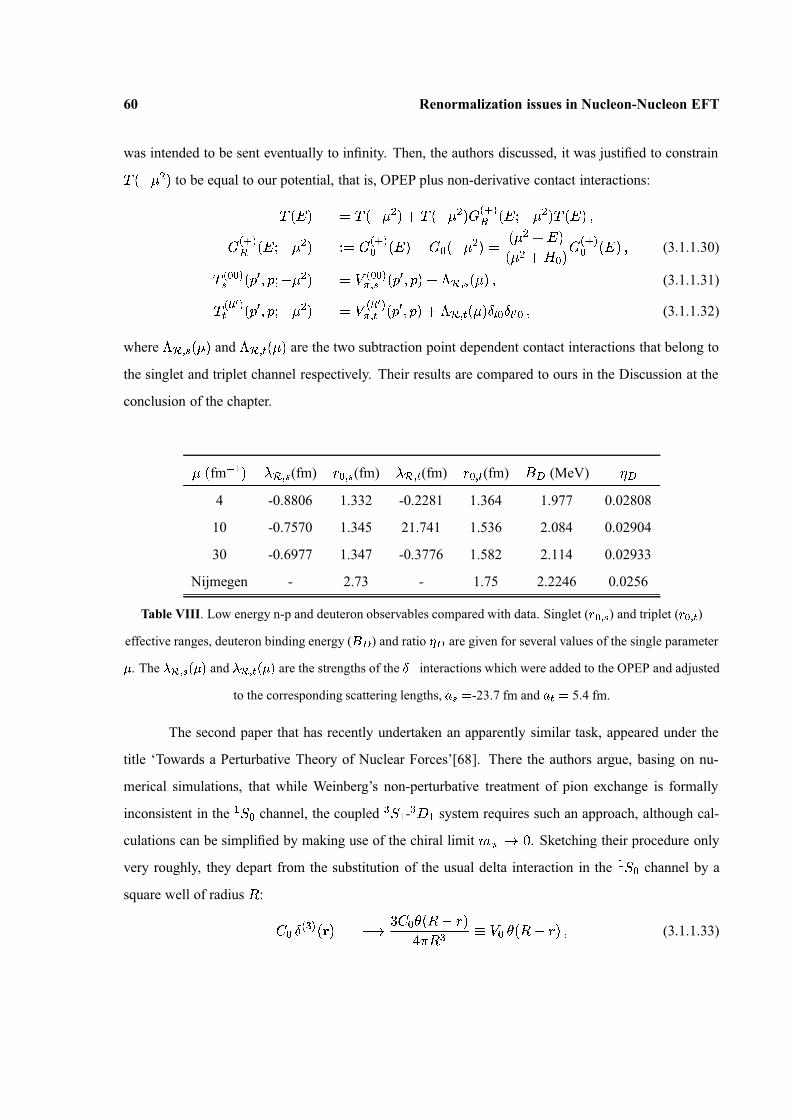
60 Renormalization issues in Nucleon-Nucleon EFT
was intended to be sent eventually to infinity. Then, the authors discussed, it was justified to constrain
� � � ��
� to be equal to our potential, that is, OPEP plus non-derivative contact interactions:
� � � � � � � � ��
� � � � � ��
�� � � �
� � � � � ��
� � � � � �
� � � �� � � � � �
��
��
� � � �� � � � �
�� � � �
�� �
� � � � � �
� � � � � � �
� � � �� � � � � (3.1.1.30)
�� � � �
� � ��
� � � � ��
� �
� � � � �� � � � �
�� � � � � � � � � � � � (3.1.1.31)
�� � � � �
� � ��
� � � � ��
� �
� � � � � �� �
� � ��
� � � � � � �
� � � � � � � � � � � � (3.1.1.32)
where � � � � � � � and � � � � � � � are the two subtraction point dependent contact interactions that belong to
the singlet and triplet channel respectively. Their results are compared to ours in the Discussion at the
conclusion of the chapter.
� � fm � �� � � � � (fm) � � � � (fm) � � � � (fm) � � � � (fm)
�� (MeV) � �
4 -0.8806 1.332 -0.2281 1.364 1.977 0.02808
10 -0.7570 1.345 21.741 1.536 2.084 0.02904
30 -0.6977 1.347 -0.3776 1.582 2.114 0.02933
Nijmegen - 2.73 - 1.75 2.2246 0.0256
Table VIII. Low energy n-p and deuteron observables compared with data. Singlet ( � � � ) and triplet ( � � � )
effective ranges, deuteron binding energy ( � ) and ratio � are given for several values of the single parameter
� . The � � � � � � and � � � � � � are the strengths of the � � interactions which were added to the OPEP and adjusted
to the corresponding scattering lengths, � � � -23.7 fm and � � � 5.4 fm.
The second paper that has recently undertaken an apparently similar task, appeared under the
title ‘Towards a Perturbative Theory of Nuclear Forces’[68]. There the authors argue, basing on nu-
merical simulations, that while Weinberg’s non-perturbative treatment of pion exchange is formally
inconsistent in the � �� channel, the coupled � �
� - �
� � system requires such an approach, although cal-
culations can be simplified by making use of the chiral limit � � ��. Sketching their procedure only
very roughly, they depart from the substitution of the usual delta interaction in the � �� channel by a
square well of radius � :
� � ��
� �� � � � �
� � � � � � � � �
� � �� �
�� � � � � � � � (3.1.1.33)
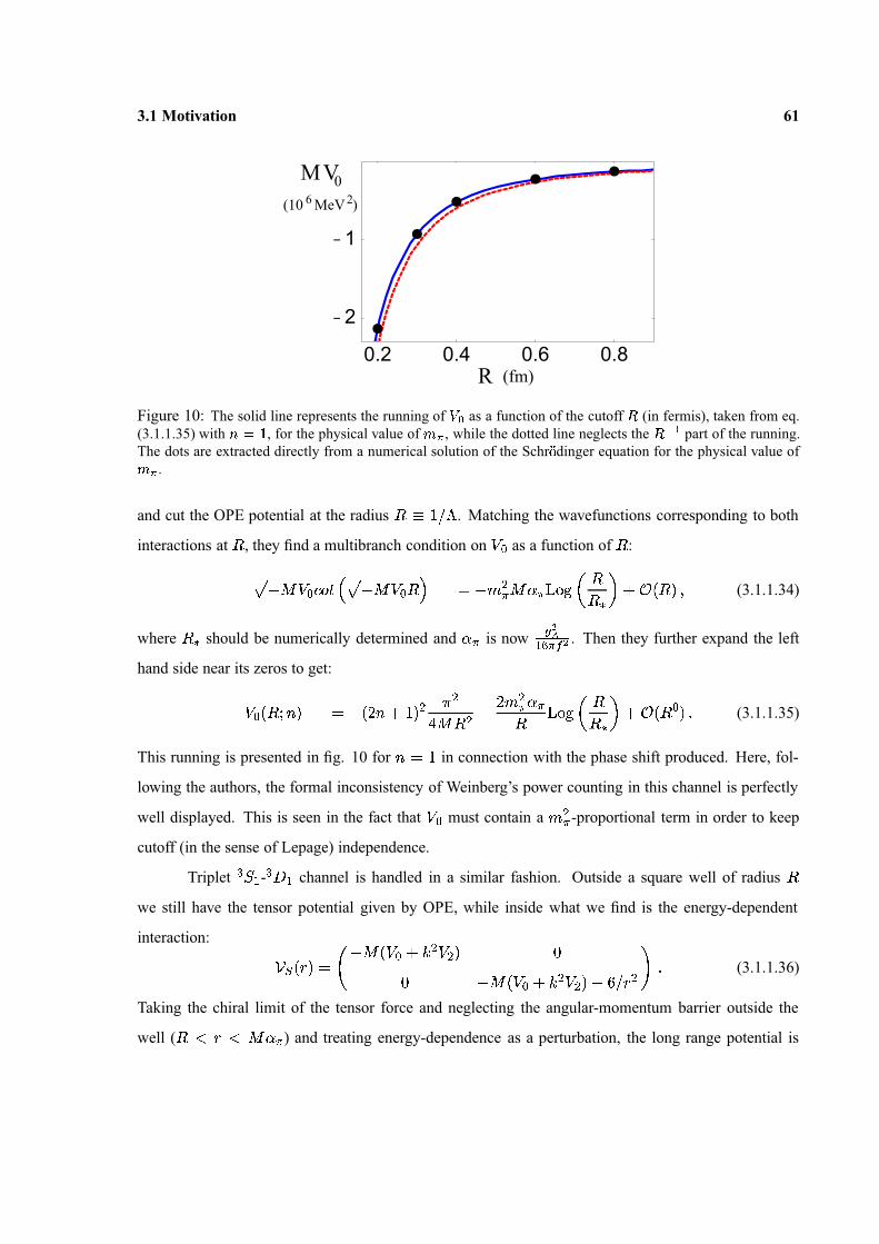
3.1 Motivation 61
0.2 0.4 0.6 0.8
-1
-2
V0M26(10 MeV )
R (fm)
Figure 10: The solid line represents the running of � � as a function of the cutoff � (in fermis), taken from eq.(3.1.1.35) with � �
�, for the physical value of �
�, while the dotted line neglects the �
� � part of the running.The dots are extracted directly from a numerical solution of the Schr �� dinger equation for the physical value of
��
.
and cut the OPE potential at the radius � �
�� � . Matching the wavefunctions corresponding to both
interactions at � , they find a multibranch condition on�
� as a function of � :
�� �
�
� � �
�� �
� �
�� � � � � �
�
� � � �
� � �
��
� � � � � � � � � (3.1.1.34)
where � � should be numerically determined and � � is now� ��
� ��
� � . Then they further expand the left
hand side near its zeros to get:
�
� � � � � � � � ��
� � ��
� ��
� � � � ��
��
� � �
�� � �
� �� � � � � � � �
� � (3.1.1.35)
This running is presented in fig. 10 for � � �in connection with the phase shift produced. Here, fol-
lowing the authors, the formal inconsistency of Weinberg’s power counting in this channel is perfectly
well displayed. This is seen in the fact that�
� must contain a ��
� -proportional term in order to keep
cutoff (in the sense of Lepage) independence.
Triplet � �� - �
� � channel is handled in a similar fashion. Outside a square well of radius �
we still have the tensor potential given by OPE, while inside what we find is the energy-dependent
interaction:�
� � � � � � � � ��
� � � ��
� ��
� � � ��
� � � ��
� � � � � � �
� � (3.1.1.36)
Taking the chiral limit of the tensor force and neglecting the angular-momentum barrier outside the
well ( � � � � � � � ) and treating energy-dependence as a perturbation, the long range potential is
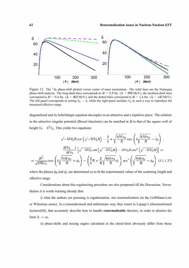
62 Renormalization issues in Nucleon-Nucleon EFT
100 200 300
20
40
60
| P | (MeV)
δ
100 200 300
20
40
60
| P | (MeV)
δ
Figure 11: The � � � phase-shift plotted versus center of mass momentum. The solid lines are the Nijmegenphase-shift analysis. The long-dash lines corresponds to � �
� �� fm. (
�� � �
�MeV.), the medium-dash lines
correspond to � �� � �
fm. (�
�� � � MeV.), and the dotted lines correspond to � �
� � �fm. (
��
� � �MeV.).
The left panel corresponds to setting ��
��, while the right panel includes �
�in such a way to reproduce the
measured effective range.
diagonalized and its Schr �� dinger equation decouples in an attractive and a repulsive piece. The solution
to the attractive singular potential (Bessel functions) can be matched at � to that of the square well of
height�
� � ��
�
� . This yields two equations:
�� �
�
� � ��
�
� �� �
�� � � �
�
��
� �� � �
� � � �
�� � � �� � �
�� � �
�� �
�
�� � �
�
��
� �� �
�� �
��
� �� �
�� � � � �
�� � �
��
�� �
� �
�� � � � �
��
�
�
� �� � � � � �
�� � � �� � �
�� � �
�� �
�� �� � �
��
� �� � �
�� �
�� �� �
�
�� � �� � �
�� � �
�� (3.1.1.37)
where the phases � � and � � are determined so to fit the experimental values of the scattering length and
effective range.
Considerations about this regularizing procedure are also postponed till the Discussion. Never-
theless it is worth warning already that:
i) what the authors are pursuing is regularization, not renormalization (in the GellMann-Low
or Wilsonian sense). In a misunderstood and unfortunate way, they resort to Lepage’s aforementioned
lectures[60], that accurately describe how to handle renormalizable theories, in order to dismiss the
limit � � � .
ii) phase-shifts and mixing angles calculated in the chiral-limit obviously differ from those

3.1 Motivation 63
0.25 0.35 0.45
-20
-10
R (fm)
V0M26(10 MeV )
0.25 0.3 0.35
10
20
V2M
R (fm)
Figure 12: The solid lines represent the running of � � � and � ��
as a function of the cutoff � , taken from eq.(3.1.1.37). The dots are extracted directly from a numerical solution of the Schr �� dinger equation. The differentbranches in the left panel correspond to a different number of nodes in the square well, i.e. an artifact of thisparticular regulator. The curves continue to smaller values of � , but we have not shown them. Further, analogousbranches exist for � �
�. For each branch, the ultraviolet phase is fit to the smallest � data point to produce the
theoretical curve.
100 200 300
100
150δ0
| P | (MeV)
100 200 300
-20
-10
δ2
| P | (MeV)
Figure 13: The � ��- � �
�phase-shifts as a function of the center of mass momentum. The solid line is the
Nijmegen phase-shift analysis. The long-dash line corresponds to � �
� � � �fm. (
��
� �� MeV.), the medium-
dash line corresponds to � �� �
��
fm. (�
� � �� MeV.), and the dotted line corresponds to � �
� � � �fm.
(�
�� � � �
MeV.). ��
was kept equal to zero.

64 Renormalization issues in Nucleon-Nucleon EFT
100 200
50
100
150
| P | (MeV)
31S
δ LO
2N LO
4N LO
6N LO
100 200
-5
-10
-153
1D
| P | (MeV)
LO
2N LO
4N LO
6N LO
100 200
2
4
| P | (MeV)
ε1LO
2N LO
4N LO
6N LO
Figure 14: The � � , � � phase-shifts and ��
mixing angle in perturbation theory out to N � LO in � � � � ��
� � � � � ��
� .The solid line is the result of the Nijmegen phase-shift analysis, while the dotted curves correspond to the LO,N � LO, N � LO and N � LO results, as indicated on each panel. These results were obtained for a square well ofradius of � �
� ��
�fm., with � � �
� � � � � � �� MeV. � and � � �
�� � �
� � � � �� .
which keep the mass of the pion finite; the expansion around � � = 0 turns out to be quite wild behaved
(see fig. 14).
Finally, we would like to stress that, in spite of the rooted beliefs of some people, also in
quantum theories the limit � � � is the relevant one (see ref. [69]).
After this brief account of related/previous work, which provides the subjective context of our
interests, we finally are in the right position to present our own contribution to the subject. In the follow-
ing pages our aim will be the making up of an analytically clear response to the concrete question: can
the One Pion Exchange Potential (OPEP) be renormalized (in the conventional sense, that is, sending
the cutoff to infinity)? We have just shown, when pursuing the tangled thread of controversies this issue
has arised, the subtlety of our, apparently, simple question. So, as we do not desire that any intricacy
of the renormalization procedure, that may deliver a valid solution, is lost due to more or less widely
accepted conjectures, we will proceed in the most general fashion. That is, we will take the OPEP
potential, will analyze its behaviour when iterated through a Lippmann-Schwinger equation and will be
so open-minded as to allow all couplings in the potentials (even the ones in front of the non-local terms)
to vary so as to absorb all cutoff dependence in the limit � � � . That is the usual3, most general
approach from a Field Theory perspective, one that, by recognizing our hopeless inability to perform a
non-perturbative matching between the NN Lagrangian and QCD, indulges to consider more freedom
than perhaps necessary. Note, however, that the standard choice ‘only local terms should renormalize3Not only it is found in theoretical works on renormalization of singular potentials (see for instance [70]), but also there are
known examples in a non-relativistic EFT of QCD (pNRQCD) where the renormalization of non-local potentials is requiredin order to absorb certain divergences [71], the most spectacular of which being the renormalization of the static potential[45, 72].

3.1 Motivation 65
divergences’ is also studied as a restricted subset in a larger ensemble of possibilities we examine.
Anyway, allowing for the renormalization of non-local potentials in the NN system should not
represent any problem, even if their coupling constants are fixed to definite values when their potentials
are computed from the HB � L. What matters for the low energy properties of NN systems is not the
precise values those constants take at the scale of the HB � L, but only the form of the potentials them-
selves. Hence, any of those (bare) constants with a non-trivial flow will just provide a free parameter
(the analogous to a renormalized coupling constant), which may be eventually fixed by low energy data
or, alternatively, related to its (higher energy) HB � L value by a matching procedure. There is no need
of elaborating further on this point because, eventually, it will not be needed. Let us only mention that
it has some implications. Mainly, it becomes irrelevant whether a certain potential, which first arises
at a given order of � PT, receives also contributions from higher orders, since this will amount to a re-
definition of (unknown) counterterms. In particular, for the lower energy EFT there is no inconsistency
at all in the so-called Weinberg counting for the � �� channel we have been referring to all during this
section. It only reflects the fact that the low energy calculation, or NN EFT, is not organized in terms of
the chiral counting anymore4.
So, as we pose this study, at the same time the regularization analysis tells us whether a con-
stant does flow, relevant information about the actual form of the cutoff dependence, as well as the way
its subleading behaviour in � enters into observables (and therefore is fixed by experiment), is easily
attained. By regarding NN renormalization as a theoretical matter, not only are we avoiding the so-
conspicuous model-dependency of previous works, but are also leading the way to a deeper insight on
the power counting and organization of the theory. That is, our results, although perhaps phenomeno-
logically less spectacular than some commonly accepted numerical treatments, are not intended to affect
their very successful achievements. Even a way of comparison is sometimes difficult, taking into ac-
count that their flows/solutions fail to consider the strict limit of � � � , which furthermore explains
why some of their observables behave more or less wildly when approaching this limit. Let us advance
right now some of the main points we reach after the next demonstration, as we regard they are worth of4In other words, HB � PT is a local theory with pions and non-relativistic nucleons as explicit degrees of theory. It has an
energy cutoff ( � � ) such that�
� � � � � � � � � � � � and a momentum cutoff ( ��
) which verifies � � �� �
� � � � � . Therefore its Lagrangian can be organized according to the chiral counting since this (and its breaking) is aexplicit symmetry. But the NN lower energy EFT we are handling has an energy cutoff ( � � ) such that
� � � � � � � anda momentum cutoff ( �
�
) such that � ��
� � � �� � � . Namely, it consists of non-relativistic nucleons interacting via a
(non local) potential. No pion fields exist and chiral counting is not a natural way to organize the theory anymore.
66 Renormalization issues in Nucleon-Nucleon EFT
being emphasized from the very beginning. It is going to be clearly shown that, in order to renormalize
the non-perturbatively handled full OPEP, the coupling ( � � ) accompanying the tensor-like, non-local
interaction describing pion exchange does need to flow so as to produce a non-trivial scattering am-
plitude. Nevertheless, we will find out that the strong cutoff dependence of � � , otherwise obliged in
order to regularize the spin conserving part of the interaction, induces as a solution a T-matrix that lacks
from partial wave mixing. This unphysical, undesirable feature leads us to conclude that, in order to
renormalize, one should distinguish between spin symmetry conserving (SS) and breaking (SSB) terms
of the interaction. While the first ones (diagonal part in a 2 � 2 matrix notation) are tagged as LO and
must be resummed, the second ones are handled out perturbatively and begin contributing at NLO. We
further demonstrate, in first order perturbation theory, that this way, no non-local term coupling constant
does need to flow. At the same time this proposal seems to be consistent with the fact that partial wave
mixings are observed to be rather small in all triplet channels. Finally, while a possible power counting
that ensures renormalizability is proposed, a future line of further study is pointed out.
3.2 A convenient decomposition
We start from the LO NN potential:
�
� � � � �� � �
� ��
�
� �� �
�� �
��
�� � � � � � �
� �� � � � � � �
�
� � � � �� � � �
��
� � � � � �� � �
�� � (3.2.1)
This potential acts on a wave function � � �� � � � � � �� , where � � � and � � � are nucleon isospin and
spin indices respectively, which can be decomposed into irreducible representations of spin and isospin
as follows:
� � �� � � � � ��
� �� �
� �� �
� �� � � �
�� � � � � � � �
� �� �
� �
�� �
� � � ��
��
� � � � � �
� � �
�
�� �
� �� �
� � � ��
�� � � � � � � �
�
�� �
� �� �
�� �
� � � ��
� ��
� � � � ��
� (3.2.2)
The potential (3.2.1) reduces for each isospin-spin channel to:
�� � � � � � �
� � � �
� � ��� � � �
� � � � ��
�
� � � � �� � � � �� � � � � � � � �
�
� � �� � � � � � �
� � �
� � ��� � � �
� � � � ��
�� � � � �
�� � � � �
� �� � � � �
�� �
� � � � �� � � � �� � � � � � � � � � � � �
�

3.2 A convenient decomposition 67
�
��
� � � � � � �� �
� � ��
� �� �
� � � � ��
�� �
�
� � � � �� � � � �
�� � � � � � � � � � �
��
��
� � �� � �
� � � � � � �� � �
� � ��� �
� �
� �� � � � � �
��
� � ��
� ��
� � � � �� � �
� � � � ��
��
� � � � �� � � � �
�� � � � � � � � � �
�� � � � �
�(3.2.3)
We still have to implement Fermi symmetry. This implies that the irreducible wave functions
(3.2.2) must fulfill (isospin and spin indices will be omitted for the rest of this section):
�� � � � � � �
�� � � � � � �
�� � � � � �
�� � � � � � �
�� � � � � �
�� � � � � � �
�� � � � � � �
�� � � � � � � (3.2.4)
which is implemented in the LS equation if we choose:
� � � � � � � �� � � �
�� � �
� � � � � � �� �
�� � � � � � � �
��
�
��
�� � � �
� ��
�� � �
� �� � � � � � � �
� ��
� � � � � � � � ��
� �
� �� � � �
� � �� � � � � � �
� � �� � � �
� � ��
� �� �
� � � � � � � �� � � �
�� � �
� � � � � � �� �
�� � � � � � � �
��
�
��
�� � � �
� ��
�� � �
� �� � � � � � � �
� ��
� � � � � � � � ��
� �
� �� � � �
� � �� � � � � � �
� � �� � � �
� ��
�� �
� �
(3.2.5)
It is the advantage of the above decomposition that we will not need to specify which (coupled) partial
waves we are analyzing.
If the LS equation for the potentials (3.2.3) was well defined, using (3.2.5) would be equivalent
to solving the LS equation:
�
� � � � � � � �� � � �
�� � � � � � �
� �� � � �
� ��
�� � �
�� � � � � � � �
�
�
� �� � � �
� � �
�
� � � � � � �� � �
� � � � (3.2.6)
( � � � =�
��
) namely, ignoring the statistics and then using the standard formulas:
� � � � � � � �� � � �
��
� �
� � � � � � � �� � � �
�
� � � � � � � � �� � � �
� ��
� �� �
� � � � � � � �� � � �
��
� �
� � � � � � � �� � � �
�
� � � � � � � � �� � � �
� ��
� �� � (3.2.7)

68 Renormalization issues in Nucleon-Nucleon EFT
However, the LS equation for�
�� � is not well defined in any channel and hence using (3.2.5)
or (3.2.6)-(3.2.7) may not be totally equivalent. In particular, for the SS and VV channels, the UV
divergences one finds using (3.2.5) are softer than those from (3.2.6)-(3.2.7), so we shall work with
(3.2.5). For the SV and VS channels, however, the UV divergences found using (3.2.5) are as strong
as the ones that stem from (3.2.6)-(3.2.7). For convenience, we have chosen to work with the latter for
these channels.
The LS equation in the isoscalar-scalar channel is already in (3.2.5) well defined, as it is apparent
from the antisymmetrization of the corresponding potential (3.2.3). On the contrary, the other three
channels require regularization. Searching for the systematics to tackle them will be the aim of the
next three sections. For notation simplicity, the energy dependence of the T-matrices as well as of other
auxiliary functions will not be displayed explicitely for the rest of the chapter.
3.3 The isovector-singlet channel
The LS equation for this channel reads:�
� ��
� � � � � � �� �
��
�� � � � � � �
� � �� � � � � ��
� � � ��
� �� � � � � � � ��
��
�
�� �
��
��
�
�
� � �� � � � � �
� � �� �
where�
��
� � � � � � �� �
�� � �
� �
� � � � �� � � � ��
�� �
��
� ��
� � � � � � � �� � ��
� �� �
�
� �
�� �
� � � � ��� �
� �
� (3.3.1)
where in the last lines we remember the values those constants will take if the potential had been
calculated at LO in � PT. The hat and the VS subscript will be dropped in the following.
Let us define:
�� � �
� � �� �
�� � � �
� ��
�� � �
� ��
� � � �� � �
�
� �
� ��
� � � (3.3.2)
Then (3.3.1) reads:
� ��
� � � � �� � � � �
��
�� � �
� � � ��
�� � � �
�
� � � � �� � � � �
��
� � � �� �
��
� � �
� �
� � � � � �� � � � �
�
� ��
� � � �� � �
�
� �
� ��
� � �(3.3.3)
3.3 The isovector-singlet channel 69
and can be rewritten after solving:
� � � � � ��
� �
�
� � � ��
� �� � �
�
�
� �
� ��
� �
��
� � �
� �
� � � �� �
� �� � ��
� � � �� �
� ��
�
� ��
� ��
� � ��
� (3.3.4)
in the form:
� � � � ��
� � � � � � � � � ��
� � � � ��
��
� ��
� �
��
� � �
� �
� ��
� �
��
� � �
� � � � � �� �
�
� ��
� ��
� � ��
� � (3.3.5)
where we have dropped the � � �structure. If
�� � �
� was a fixed function, the equation above would be
well defined and could already be solved with no need to regularize it. However�
� � �� is a functional
of � and a second equation which relates them must be introduced. This is achieved by multiplying
eq.(3.3.5) by� � � � �
� �� � � � � and integrating over � . We obtain:
� � �� � �
� � �� � �
� � � � ��
� ���
� � � �� � � � � �
� ��
�
� ��
�� �
�� � � � � � � � � �
�� � ��
� � � � ��
� � � � ��� � � � �
� �� �
�
�� �
� � � � � � � ��
�� �
�� �
��
�� �
� �
� �
��
� �
� ��
�� � �
�
� �� �� � � �
� (3.3.6)
Substituting iteratively � � in (3.3.4) in the rhs of (3.3.6) we see that only the first iteration
produces further divergent expressions when � � � . We can then write (3.3.6) as:
� � �� � �
� ��
� � �� � � �
�� � �
��
� � � � � � � � �
� � � �
� � � � (3.3.7)
where � � and�
contain linearly and logarithmically divergent terms respectively, whereas�
(� �
) just
denote finite functions:
� ��
� �
� ��
�� � �
� �
� � � �
��
� � �
�
� �� �� � � �
�
� � � � � �� � � � ��
�
� ��
� ��
� � � ��
�� � �
��
�� �
� ��
�� � �
� � � � � � ��
� �� �� � � �
�
� � ��
� �
� ��
�� � �
� �
� � � �
��
� � �
� �
� � � � �
��
� � �
�
� �� �� � � �
� �
� � � � � �� � � � ��
� � � � � �� � � � �
�
� ��
� ��� � � �
�
� ��
� � ��
� � � �(3.3.8)
It is clear that the expression (3.3.7) can be renormalized by a redefinition of � � . In dimensional
regularization, (D=3+2 � ), we obtain:�
� �
� ��
� � �
� � � �
� �
�� � � � � � �
�
��� � � �
�
� �� �
��
� �� � � � �
� � � � � � � (3.3.9)
70 Renormalization issues in Nucleon-Nucleon EFT
which is in agreement with [63], as was anticipated after (3.1.1.21), and for a hard cutoff:�
� �
� �� �
�
��
��
� � �
��
��
� � � � ��
� �� �
�
��
� � � �� (3.3.10)
If we now wish to solve numerically the LS equation, we should proceed as usual and introduce
a hard cutoff. However � � is not to be fitted to the experimental data but substituted by (3.3.10) and
the cutoff made as large as possible (in practice it should be enough if � � � � � is of the order of
neglected subleading contributions from the NLO potential. What we have just proved is that the result
will be cutoff independent up to corrections � � � � � . � must be fixed at the relevant momentum scale
� � � � � � � � � � and ��
� � � � tuned to fit the experimental data.
Although we have no prediction for ��
� � � � we can try to understand from (3.3.10) how large
scattering lengths may arise. Since ��
� � � � evolves according to a non-perturbative renormalization group
(RG) equation it might take very different values depending on the scale it is evaluated at. After solving
it:
��
� � � � ��
�
� � � � ��
�� � � � � �
� �� � �
� � � �� � � �
� �� (3.3.11)
if we input the value ��
� � � � � � � ��� �
� �� �
� (3.1.1.21), we obtain ��
� � � � � � ��
� �
�
� �� �
� , which is not
quite at the natural scale ( � � ). Hence, the non-perturbative low energy dynamics does not seem to
be enough to fill the gap between the natural scales and the large scattering lengths. In spite of that, the
variation of ��
� � � � from � � to � is large enough as to justify a non-perturbative treatment of the OPE
in this channel.
3.4 The isosinglet-vector channel
The LS equation for this channel reads:�
� ��
� � � � � � �� �
��
�� � � � � � �
� � �� � � � � ��
� � � ��
� �� � � � � � � ��
�� �
�� �
��
��
�
�
� � �� � � � � �
� � �� �
where�
��
� � � � � � �� �
�� � �
� �
� � � � �� � � � ��
�� �
�� � �
� � � � �� � � � � � �
��
� � � � �� � � � �� �
� ��
� � � � � � � �
� � �� � � �
�
3.4 The isosinglet-vector channel 71
� ��
� �� � � ��
� � � �
�
� �
�� � �
� � � � ��� � � �
� (3.4.1)
where we show also the LO values of the coupling constants. We shall drop the subscript� �
and
the hat in the following. We call the term proportional to � � above spin symmetry breaking (SSB)
term. This term breaks orbital angular momentum conservation and makes the analysis of this channel
qualitatively different from the previous one. In order to illustrate it, let us take � �� � for simplicity.
As we regulate (3.4.1), the possible divergences arising when the regulator is removed depend on the
high momentum behaviour of � ��
� � � . If � ��
� � � � � � ��
, the usual power counting arguments imply
that, due to the SSB term, the integral on the rhs will rise this power by one. Hence, the high momentum
behaviour of the lhs of the equation will not match the one of its rhs unless:
1. � � ��
and the high momentum contribution of the potential cancels out the one arising from
the integral;
2. � ��
and the bare coupling constant � � goes to zero as the cutoff goes to infinity, which removes
the � � �� � � term on the rhs.
We prove in the Appendix E that the case 1. in fact reduces to 2.
So in next subsection we will proceed keeping in mind that � � ��
in some, at the moment
undetermined, way. After having explored the consequences this flow has on the amplitude, we will
examine in subsection 3.4.2 the alternative of treating SSB as a perturbation. In such a case we find that
� � is not required to depend on the cutoff.
3.4.1 Non-perturbative treatment of the SSB term
Let us then return to equation (3.4.1). It has the following structure:
� ��
� � � � �� � � � � � �
��
��
�� �
�� � � � �
�� � � �
�� � � � � �
��
�
� � � ��
� � � � ��
� � ��
� � � ��
� � �
� � �
� ��
� � � ��
� � � � ��
� � �
� �
� ��
� �
��
� � �
�
� � � �� �
� � � � ��
� ��
� �� �
� ��
�
� ��
� ��
� � � ��
��
�� �
�� �
� �
� ��
��
� � �
� ��
� � � ��
�
� �� �
� � � ��
72 Renormalization issues in Nucleon-Nucleon EFT
� ��
� � � ��
� �
� �
� ��
� �
��
� � �
� � � �� �
� � � � � �� �
� �
� � � �� �
� � � � ��
� �
�� �
� �� �
��
� ��
� ��
� � � �� (3.4.1.1)
Let us define:
� ��
� � � ��
��
� � � � � ��
��
��
� ��
� � � � � � � � � � � ��
� � � � ��
� � � � � � � � � ��
� � ��
�
� � � � � ��
� � �
� �
� ��
� �
��
� � �
�
� � � �� �
� � � � ��
� � � �� �
�
� ��
� ��
� � � ��
� ��
� � � � ��
� �� � � �
�� � � � � �
��
�
� � � ��
� � � � ��� � �
�� � � �
�� � � �
� �
��
�� �
��
� � �
�
� � � �� �
� � � � ��
� ��
� � �� �
� ��
�
� ��
� ��
� � � ��
� � � � � ��
� ��
� � � ��
� � � � ��� � �
� �
� ��
� �
��
� � �
�
� � � �� �
� � � � ��
� � � �� �
� ��
�
� ��
� ��
� � � �� (3.4.1.2)
which allows us to isolate in � ��
� � � � ��
� and � � � � ��
��
��
� ��
� � all sources of divergent behaviour, since
� � � � � and � � � � � ��
� are perfectly well defined.
Using the expressions of � ��
� � � ��
� in (3.4.1.1) and � ��
� � � ��
� in (3.4.1.2), � ��
� � � � ��
� can be
recasted in the form:
� ��
� � � � ��
� � � � � � �
��
��
�� �
�� � � � �� � � � � � � �
�
� � � � � ��
� � � � � ��
� � � � � ��
� �
� ��
� � � � � �� �
� ��
� �
��
� � �
� � � �� �
� � � � � �� �
��
� � � �� �
� � � � ��
� � � �� �
�
� ��
� ��
� � � ��
�
� �
� ��
� �
��
� � �
� � � � � �� �
� � � � � �� �
� � � � � � � �
� � � �� �
� � � � ��
� �
�
� � � �� �
�
� ��
� ��
� � � ��
� ��
� � � � � ��
� �� � � �
�� � � � � �
��
�
� � � ��
� � � � ���
� �
� ��
� �
��
� � �
� � � � � �� �
� � � � � �� �
� � � � � � � �
� � � �� �
� � � � ��
� �
�
� � � �� �
� ��
�
� ��
� ��
� � � ��
� ��
� � � � � ��
� �� �
� ��
� �
��
� � �
� � � �� �
� � � � � �� �
��
� � � �� �
� � � � ��
� � � �� �
� ��
�
� ��
� ��
� � � ��
�
� �
� ��
� �
��
� � �
� � � � � �� �
� � � � � �� �
� � � � � � � �
� � � �� �
� � � � ��
� �
�
� � � �� �
� ��
�
� ��
� ��
� � � �� (3.4.1.3)
This decomposition enables us to compute � � � � ��
��
��
� ��
� � , and hence the full amplitude
� ��
� � � ��
� , in terms of � � � � � , � ��
� � � � � ��
� ( � ��
��
��) and � � � � � �
�� through the equation:
�� � �
� �
�� �
� ��
��
� � �
� � � � � � � �
� �� �� � � �
� � �� �
� ��
��
� � �
� � �� � � � �
� �� �
� � � �� � � � � �
��
��
�� �
�� � �
� � ��
� � �� �
� ��
��
� � �
� ��
� � � � � ��
� � � � � ��
� � � � � ��
�
� �� �
� � � �� � �
� �
� ��
��
� � �
� � � � � ��
� � ��
� �� �� � � �
� (3.4.1.4)
3.4 The isosinglet-vector channel 73
As we have already mentioned � � � � � and � � � � � � �� are finite when the cutoff is removed. If
we solve � ��
� � � � � � �� , � �
��
��
�iteratively, the most divergent pieces in the � -th iteration are � � � �
� � � � ��
� , � � � � � � � � �� and � � � � � � � � �
� �� � � . These series are expected to have a finite radius of
convergence. The radius of convergence is in any case non-zero because they are bounded by geometric
series (or derivatives of them). If � � does not go to zero as�
� � or stronger (in particular, if � � is not
allowed to flow), each series will separately diverge. In that case, a finite result can only be obtained if
non-trivial cancellations occur for all � , which we do not see how they could actually happen. If, on the
contrary,
� � � � � � �
� ��
� � � � � (3.4.1.5)
and�
� � is small enough, the series will converge. For the T-matrix, such a strong cutoff dependence
implies that the terms:
� � � ��
� � � � � � �� �
� �� � � �
��
��
�� � � � �
�� � � � �
� � � ��
� � � � � � �� � �
��
�� � � � � � �
�
�� � � � �
� � � ��
� � � � � � �� � �
��
�� � � � � � �
�
�� � � � � (3.4.1.6)
where � �� �
� � is simply a finite constant and, as we see, all � , � �-encoded information will be washed out
from the amplitude.
That is to say:
� ��
� � � � �� �
� � �� � � � � � � � �
�� � �
� � �� �
�� � � � � � � � � � � � � �� � � � � � � � � � �
�� � � � � � �
� � � �
�� � � � � � �
� � ��
�
� � � � ��
� � � � � � �� � � � � � � �
��
��
�� � �
� ��
� � � � � � � �� �
� �� � � � � � � � � � � � �
� � ��
� (3.4.1.7)
which is finite provided � � � � ��
��
��
� � �� � is finite. In order to prove the latter we borrow from section
3 the following results:
� � �
��
� � �
� � � � �
� � � �� � �
� �� ��
� � ��
� � �
��
� �
� � � � ��
� �� � � �
�� �
� � �
��
� � �
� � � � � � ��
� � � �� � �
� � ��
� � (3.4.1.8)
74 Renormalization issues in Nucleon-Nucleon EFT
and find in Appendix F:
� �� �
��
�
��
� � �
� � �� � � � �
� � ��
� � � �� � � � � � � � � � � � � �
� � ��
�
� � � � �� �
�� �
� �� �
��
�
��
� � �
� � �� � � � � ��
�
� � � �� � � �
� � ��
� �
� �� �
��
�
��
� � �
� � �� � � � � ��
�
� � � �� � � �
� �� �
�� � (3.4.1.9)
where � � , � � , � � are cutoff independent constants related to�
� � . Then the flow:�
� �� �
� ��� � �
� � �
��
�� � �
��
� �
� � � � ��
� �� �
� �� � � � � ��
� �� �
�
��
� � � �� (3.4.1.10)
makes � � � � ��
��
��
� ��
� � finite and hence does (3.4.1.7). We have then proved that the flows (3.4.1.5)
and (3.4.1.10) renormalize the triplet channel.
It is not difficult to see that the various series above involving divergent terms are bounded by
geometric series or derivatives of them. This ensures that our flows provide actually finite expressions
for the amplitude if�
� � is small enough. However, this amplitude appears to be diagonal in spin space
and hence orbital angular momentum is conserved. Although, the observed � �� - �
� � mixing, which is
small, might be attributed to a higher order effect, it is clear from ref. [62] that it is due to the OPE to
a large extend. In order to preclude the conservation of orbital angular momentum, we can foresee two
ways out:
1. a SSB term may survive in the renormalized amplitude if�
� � is tuned infinitely close to the radius
of convergence of the series, so that our bounds do not hold anymore, and
2. the SSB term from OPE must be treated as a perturbation and renormalized as such.
The possibility 1. is examined in Appendix G where we show it unlikely to be realized. In the following
subsection we explore 2. and prove that if a suitable SSB term is treated as a perturbation, the amplitude
is renormalizable at first order and the mixing survives.
3.4.2 Treating the SSB term perturbatively
Let us split the potential as:�
��
� � � � �� �
� �� � �
�� � � � �
� �� �
� � ��
� � � � �� �
3.4 The isosinglet-vector channel 75
� �� � �
�� � � � �
� �
� �
� � �
�
� �
� � � � �� � � � �
�
�� �
��
� � � � ��
� � � � �� �
�
� �� � � � �
� � � � � � ��
��
� ��
�� � �
� � ��
� � � � �� � � � �
�
�
�
� �
�� � � � � � �
� � ��� �
� �
�
�
� ��
� ��
� � ��� �
� �
�
�
� �
�� �
� � � � ��� �
� �
� (3.4.2.1)
with LO values for the coupling constants indicated. In the following we drop the SV-channel subindexes.
The amplitude will be written as:
� ��
� � � � �� � �
�� � �
�� � � � �
� � �� � � �
�� � � � �
� � (3.4.2.2)
where ��
� � ��
� � � � �� fulfills:
��
� � ��
� � � � �� �
� �� � �
�� � � � �
� �� � � � �
� ��
�� � �
� �� � � � � � � � � �
�
�
� ��
� ��
� � � ��
�� �
�
�� � � �
� � �� (3.4.2.3)
The renormalized solution to this equation is given by ��
� � ��
� � � � �� � � � � � � �
� � ��
in section
3.3. At first order in perturbation theory �� � � �
�� � � � �
� verifies:
�� � � �
�� � � � �
� �� � � � �
�� � � � �
� �� � � � �
� ��
�� � �
� � � � � � � � � � � ��
�
� ��
� ��
� � � ��
�� �
�
�� � � �
� � �� �
�� � � � �
� ��
�� � �
� �� �
� � � � � � � ��
�
� ��
� ��
� � � ��
� � ��
�� � � �
� � �� (3.4.2.4)
Using (3.3.4) and (3.3.5) we can see that the second term above is finite. We can then gather the
first and second terms into a new, energy dependent, potential defined as:�� � � � �
�� � � � � �
��
�� � � � �
�� � � � �
� �� � � � �
� ��
�� � �
� � � � � � � � � � � ��
�
� ��
� ��
� � � ��
�� �
�
�� � � �
� � �� (3.4.2.5)
Therefore, the integral equation reduces to:
�� � � �
�� � � � �
� �
�� � � � ��
� � � � � �� �
�
� �
��
�� � �
� �� � � � �
� ��
�� � �
�
� �
� � � � � �� � � � ��
�� � � �
�� � � �
� � ��
� ��
� ��
� � � ��
��
�� � �
��
�� � � � �
� ��
�� � �
�� � � �
�� � � �
� � ��
� ��
� ��
� � � � (3.4.2.6)

76 Renormalization issues in Nucleon-Nucleon EFT
In order to prove it finite we decompose:
�
� � ��
�� � � � �
� ��
� �
��
�� � �
� � � �� � � � �
�
� ��
� � � � � �� � (3.4.2.7)
with � ��
� � � � defined in (3.4.1.2) and�
� ��
� � � � � �� given by:
�
� ��
� � � � � ��
��
�� � � ��
�� � � � � �
� �
� � � ��
� ��
�
� � �
�
� �
� � � � � �� � � � ��
�
� ��
� � � � �� � �
�
� ��
� ��
� � � �� (3.4.2.8)
Both � ��
� � � � and�
� ��
� � � � � �� are well defined (the tensor structure is crucial for the latter to be
so). Divergences can only arise in�
� �
��
�� � �
� , which reads:
�
� �
��
�� � �
� � �
� ���
� � � �
�
�
� �
�� �
��
� �� �
� ��
��
�
�
� � �� � �
� �� � ��
� � � ��
� ��
� � �� �
� ��
��
�
� (3.4.2.9)
The numerator is well defined (for that the tensor structure is again crucial) and the divergences
in the denominator have exactly the same structure as in the denominator of (3.3.7). Hence they are
renormalized by the same � � flows. We have then proved that if we treat the SSB term as a perturbation,
the amplitude is renormalizable at first order in perturbation theory and no extra counterterm needs to
be introduced.
3.5 Isovector-vector channel
If we use (3.2.6)-(3.2.7) in order to obtain � � � � � � � �� , the calculation of
�
� � � � � � � �� would
reduce to that of the previous section. However, as mentioned in section 3.2, the UV behaviour is
smoother in terms of (3.2.5), as it happens in the SS channel, although here we still need to introduce a
regularization. The LS equation, dropping de isospin delta, reads:
� ��
� � � � � � �� �
�� �
��
� � � � � � �� �
� � � ��
� ��
�� � �
�� �
� �� � � � � � � ��
�
� ��
� ��
� � � �� �
�� � � � � �
� � �� � (3.5.1)
where:
�� �
��
� � � � � � �� �
��
� ��
�� � � � � � �
� ��
��
� � � � � � � �� �
� �� � � � � � �� � � � � � �
��
� � � � �� � � � ��
�� � � � �
� � � � � � ��
�
� � � � �� � � � ��
� �
�� �� � � �
�
� � � � �� � � � ��
�� �
�
� � � � �� � � � ��
� � (3.5.2)
3.6 Discussion 77
where those constants calculated at first in � PT take the values:
� ��
�
�� � �
�
� �� �
�
� �
��
� � � � ��� �
� �
� (3.5.3)
We have not analyzed the possible existence of non-trivial flows which may renormalize the
above equation. The fact that the SSB term must be treated perturbatively in the SV channel, indicates
that also here we should proceed according to the same philosophy. The potential (3.5.2) in the zeroth
order approximation reads:� �
� � � ��
� � � � � � �� �
� �� � � ��
� � � � �� � � � ��
�� �
�
� � � � �� � � � ��
� � (3.5.4)
which leads to a well defined LS equation. At first order in perturbation theory we will have:
� ��
� � � � � � �� � �
�� � �
�
� � � � � � �� � �
�� � �
�
� � � � � � �� �
��
� � ��
� � � � � � �� �
� �� � �
�
� � � � � � �� �
� � � � �� �
��
� � �
� �� � � �� � � � � � � �
��
�� �
�
�
� � � � � �� � �
�
� ��
� ��
� � � ��
�� � � � �
� ��
�� � �
� �� � � �� � � � � � � �
��
�� �
�
�
� � � � � �� � �
�
� �
�� �
�� � � �
� (3.5.5)
which is also well defined. We expect the divergences arising at higher order to be absorbed by local
counterterms.
3.6 Discussion
We have addressed the renormalization of the LS equation for the LO potentials (in the � PT
counting) of the NN system in all channels. In addition, for each channel we have been able to carry out
our analysis for all partial waves (including partial wave mixing) at once. The isoscalar scalar channel
does not require regularization. For the isovector scalar channel we recover the flows of ref. [63]. The
remaining two channels have deserved a more detailed study.
The first non-trivial result is that the renormalization of the isoscalar vector channel requires a
strong flow of the coupling constant of a non-local potential, the SSB one, or, in other words, if only
the coupling constants of the local potentials are allowed to flow, the isoscalar vector channel is not
renormalizable. Several comments are in order.
78 Renormalization issues in Nucleon-Nucleon EFT
First of all, the flow (3.4.1.5) of the coupling constant of the SSB term is not such a big surprise.
Notice that at high momentum this term tends to a (direction dependent) constant, which is the same
behaviour (except for the direction dependence) as the � -function term both in the singlet and the triplet
channel, the coupling constants of which also show similar flows. The main difference is that the
leading behaviour for � � is fixed and the subleading contains the free parameter ( ��
� � � � ). For � � instead,
the leading behaviour contains the free parameter (�
� � ) and the subleading behaviour is not observable.
The flow (3.4.1.5), however, has undesirable consequences: the renormalized T-matrix con-
serves orbital angular momentum, even if the bare interaction does not (see Appendix G)5. Since the
results of [62] indicate that it is precisely the OPE the main responsible for the mixing of higher partial
waves, we would like it to keep doing this job for us. We are then forced to exclude the SSB term from
the (low energy) LO potential, and to treat it as a perturbation. This also appears to be reasonable from
the phenomenological point of view since the observed mixings are small[62].
We have developed this line in sections 4.2 and 5. We have proved that at first order the vector
channels remain renormalizable (at zeroth order the problem reduces to the one in the singlet channels,
which are renormalizable). The picture which emerges is half way between [64], where the pions
are treated perturbatively, and [61, 74] where the whole potential is treated non-perturbatively. The
(low energy) LO potential is the part of the LO potential in the � PT counting which conserves orbital
angular momentum. We are tempted to propose the following counting. The � � ��
� ( � ��
��
� � � � �
contribution to the NN potential in the � PT counting must be divided into two pieces: the one which
conserves orbital angular momentum (SS) and the one which does not (SSB). The SSB terms keep their
� PT counting but the SS ones are enhanced and must be counted as � � ��
��
� . Only the LO potential
� � � ��
� must be treated (and renormalized) non-perturbatively. We have seen here that this proposal
is theoretically consistent at next to leading order, and, in addition, it does not require any coupling
constant of a non-local potential to flow anymore. It remains to be seen if it is still so beyond that order
and, of course, whether it is phenomenologically successful.
Let us finally comment on recent work on the subject [67, 68]. The authors in both references
try to renormalize the triplet channel by adjusting the coupling constant of the � -potential only. Hence,
5We have also checked perturbatively in �
� � and � � up to order �
� � � � that the effective range depends on �
� � only through thescattering length. Since the latter can be adjusted by tuning �
�
� � � � , up to this order both the scattering length and the effectiverange are blind to �
� � . We have not looked at what happens to the rest of the amplitude or to higher orders but we suspect thatthey are also insensitive to �
� � .
3.6 Discussion 79
according to our results both works should show a remnant cutoff dependence when the cutoff is large
enough. Note also that it is only in the large cutoff limit when a meaningful comparison is possible,
since the regularizations used in the three works are different.
The authors of ref. [67], who use a subtracted ( � -dependent) LS equation, argue that a rea-
sonable boundary condition is that for large � the T-matrix coincides with the potential, and check
numerically whether, once the scattering lengths are fixed, the remaining observables are independent
of � for large � . They find that for laboratory energies up to 100 MeV. the � �� and �
�� phase shifts
are remarkably independent of � for �� 0.8 GeV. but the mixing angle shows a strong � -dependence
for 6 GeV. ��
� 0.8 GeV. and only for �� 6 GeV. the � -dependence smooths and the results may
appear to converge. We interpret this stronger � -dependence of the mixing angle as an indication of the
remnant cutoff dependence mentioned above.
The authors of ref. [68] obtain the flows by analyzing the short distance behaviour of the
Schrodinger equation (see also [73]). For the � �� channel they are in qualitative agreement with ours.
For the triplet one they present analytic flow equations which are argued to coincide with those of the
chiral limit. The flow of the � -function term is given implicitly by their equation (18). They assume
that their � � , which is proportional to our � � , does not flow6 and find a multibranch structure for the
flow of their�
� � � , which is proportional to our � � ( � � �, � playing the role of an inverse cutoff). It
is interesting to note that if they allowed � � flow like our � � in section 4.1, namely � � � � , and�
� � �
like our � � , namely�
� ��
� � � , their eq. (18) becomes cutoff independent. Hence our flow (4.1.5) is
a solution in the � � �limit to the flow equation (18) of ref. [68]. Recall, however that, if � � is not
allowed to flow, the strict limit � � �cannot be taken. More precisely, it is not difficult to prove that
there is no continuous solution to this equation for � � �(see Appendix H). Hence eq. (18) of [68]
does not produce any acceptable flow for�
� and, therefore, it cannot be used to properly renormalize7
the triplet channel.
Furthermore, we would like to remark that leaving the cutoff finite and checking that the finite
cutoff effects are higher order in the EFT expansion is a procedure which unavoidably will lead to
problems in this case. If we wish to improve the accuracy of our EFT calculation, we will have to
6Whereas the combination�
� ��� that appears in the singlet channel is equivalent to out � � and, accordingly, remains
fixed.7We use here the standard meaning of renormalization in quantum field theory, namely that the cutoff can be taken
arbitrarily large (like, for instance, in refs. [63, 64, 67, 69]).

80 Renormalization issues in Nucleon-Nucleon EFT
calculate at higher orders. Even if we insist in keeping � finite, we will have to choose it smaller and
smaller for the LO terms not to jeopardize the accuracy of the higher order calculation. Then, at some
point, � will hit the region were no continuous solution exists and we will loose all predictive power (if
we give up continuity, an infinite number of inequivalent solutions exists).
Chapter 4
New predictions for inclusive
heavy-quarkonium P-wave decays
4.1 Motivation
Inclusive P-wave decays to light hadrons have proved to be an optimal testing ground of our un-
derstanding of heavy quarkonia. The underlying assumption was that in such systems, the annihilation
of the heavy quark and antiquark is a short distance process. Set by the scale of the heavy quark mass
� , it provides with some Wilson coefficients which, because of the asymptotic freedom of QCD, can
be computed in perturbation theory. Whereas, the bound state dynamics is factorized and accurately
described by means of a lower energy EFT, originally NRQCD[76, 77]. This is a non-relativistic field
theory for the heavy quark and antiquark that is coupled to the usual relativistic field theory for light
quarks and gluons. The theory is made equivalent to full QCD through the addition of local interactions
that incorporate relativistic corrections to any order in the heavy-quark velocity � ��. The Lagrangian
for NRQCD is:
��
�� � � � � � �
��
�
�
� � ��
�
�� � � � � � �
�� � �
�� �
� � � � � � �� � �� �
�� � � (4.1.1)
��
��
�
� �� � � � � � �
�
�
�
� � � �
� � � � � �
�
�
�
� � � (4.1.2)
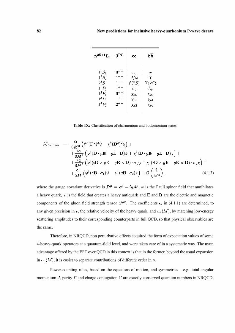
82 New predictions for inclusive heavy-quarkonium P-wave decays
� � � � � � � � � � � �
� � ��
��
�� � �
�� � �
��
� ��
�� �
�� �
��
� ��
�� �
��
�� �
�� � � �
� �� � � � �
� � � �
� � �� � � � � �
� � � �� � �
� � � � � �� � � �
� � �� � � � � �
Table IX: Classification of charmonium and bottomonium states.
��
� � � � ��
� � �� �
��
�
� � ��
�
��
� �� �
��
�
��
�� � �
� � �
��
�
� � ��
��
� � � � ��
��
� � ��
��
�� � � � �
��
� � � �� � �
��
�
� � �� �
��
� � � � ��
�� �
� �� � �
�� �
��
� � � � ��
�� �
�� � � �
� � ���
� � �� � �
�� � �
�� �
�� � �
��
� � � � � �� �
�� � � (4.1.3)
where the gauge covariant derivative is � � � � �� ,
�is the Pauli spinor field that annihilates
a heavy quark, � is the field that creates a heavy antiquark and � and � are the electric and magnetic
components of the gluon field strength tensor� � . The coefficients � � in (4.1.1) are determined, to
any given precision in � , the relative velocity of the heavy quark, and � � � � � , by matching low-energy
scattering amplitudes to their corresponding counterparts in full QCD, so that physical observables are
the same.
Therefore, in NRQCD, non perturbative effects acquired the form of expectation values of some
4-heavy-quark operators at a quantum-field level, and were taken care of in a systematic way. The main
advantage offered by the EFT over QCD in this context is that in the former, beyond the usual expansion
in � � � � � , it is easier to separate contributions of different order in � .
Power-counting rules, based on the equations of motion, and symmetries – e.g. total angular
momentum�
, parity � and charge conjugation � are exactly conserved quantum numbers in NRQCD,

4.1 Motivation 83
while there is an approximate heavy-quark spin symmetry–, allowed for a recognition of those terms that
contributed to a given process. Take a heavy meson � � � , whose dominant component is a pure quark-
antiquark state � � �� � . There, the Fock state which contains a dynamical gluon, � � �� � � , is suppressed by
a power of �� . Its angular momentum state can be denoted by the spectroscopic notation � �
� �� � , which
means it has parity � = � � ��
� � � and, if it is in a colour-singlet state, charge-conjugation number �= � � �
�� �
� . Conservation of� � � means that mixing is allowed only between the angular-momentum
states ��
�� �
� � and ��
� � �� � . However, such mixing is suppressed because operators that change
orbital angular momentum must contain at least one power of � � .
As was stated by the authors of [76], in contrast to the S-wave states, Fock states containing
dynamical gluons may play an important role in P-wave annihilation decays. The argument went like
this: the� �
� state � � � � consists predominantly of the Fock state � � �� � , with the � �� pair in a colour-
singlet � � � state but it has a probability of order � � for the Fock state � � �� � � , with the � �� pair in a
colour-octet � �� or �
� � state. As the Fock state � � �� � is created and annihilated by the dimension-8
operator � � �� � � � �
� � �� ��
�� � � �
� �� ��
�� � , the Fock state � � �� � � , with the � �� in a colour-
octet � �� state, also contributes to the decay at the same order in � through the operator � � �
� �� � �
� �� �
� ��
� � �. The resulting expression for the decay rates were said to be of the form:
�� � � � � � � �
��
� � � �� � � �
�� � � � � � � �
� � � � � � � � � ��
� � � �� �
� �
�� � � � � � � �
� �� � � � � � � � � �
� �� �
�� � � � � � � � �
��
� � � �� � � �
�� � � � � � � � �
� � � � � � � � � � ��
� � � �� �
� �
�� � � � � � � � �
� �� � � � � � � � � � �
� �� (4.1.4)
Furthermore, singlet matrix elements could be easily understood in terms of the non-relativistic Coulomb-
gauge radial wavefunctions. Defined as:
� � � � � �
�
� � �
�
�
��
�� �
�� �
� ��
�� � ��
��� � � � � � � �
�
� �
�
� � � (4.1.5)
and so on, use could be made of relations such as:
�� � � � � �
� �� � � � � � � �
���
� � � � ��
� � � � � ��
� � �
��
� � � �� �
� � ��
� � ���
�� � � �
�� � � � � �
�� � �
�� � � � � �
� �� � � � � � � � �
���
� � � � ��� � � � �
� � � � � ��
� � �
��
� � � �� �
� � ��
� � � ���
�� � � � ��
� � � � �� � � � � �
�� � �
84 New predictions for inclusive heavy-quarkonium P-wave decays
� � � � � � ��
� � � � � � � ��
��
�
�
� ��
� ��
� �� � � �
�� � �
� � � � � � � ��
� � � � � � � � ��
��
�
�
� ��� �
�� �
� � � �
�� � � (4.1.6)
which require from the use of the vacuum-saturation approximation and where some wave functions
have been replaced by their weighted average � � , without any loss of accuracy.
Nevertheless, besides the so-called colour-singlet operators, for which their expectation values
could be related to wave functions in an intuitive way, there were also colour-octet operators. The
latter were decisive in solving the infrared sensitivity of earlier calculations[78]1. It was thought that
these colour-octet expectation values could not be related with a Schrodinger-like formulation in any
way. In the following it will be shown that it is not so. For certain states, those in which a potential
description applies, the expectation values of colour-octet operators can also be written in terms of wave
functions and additional bound-state-independent non-perturbative parameters. We shall focus on the
operators relevant to P-wave decays into light hadrons, but it should become apparent that this is a
general feature[79].
The line of developments that led us to this result is the following. It was pointed out in ref.[75]
that NRQCD still contains dynamical scales, which are not relevant to the kinematical situation of the
lower-lying states in heavy quarkonium, whose energy scale is ultrasoft ( � � �� ). Hence, further
simplifications occur if we integrate them out. We call pNRQCD the resulting effective field theory[40,
41]. When the typical scale of non-perturbative physics, say � � �� , is smaller than the soft scale � � ,
and larger than the ultrasoft scale � �� , the soft scale can be integrated out perturbatively. This leads to
an intermediate EFT that contains, besides the singlet, also octet fields and ultrasoft gluons as dynamical
degrees of freedom [45, 75]. These are eventually integrated out by the (non-perturbative) matching
to pNRQCD [45]. When � � �� is of the order of the soft scale, the (non-perturbative) matching to
pNRQCD has to be done in one single step. This framework has been developed in a systematic way in
refs. [40, 41].
1That is, the infrared logs encountered in those coefficients accompanying the colour-singlet terms, are cancelled by theultraviolet behaviour of colour-octet operators.
4.2 Computation 85
4.2 Computation
Then, we will compute the inclusive P-wave decay widths into light hadrons at leading order for
� � �� �
� � � by using pNRQCD. In this situation the singlet is the only dynamical field in pNRQCD
(Goldstone bosons are also present, but they play a negligible role in the present analysis and will be
ignored), if hybrids and other degrees of freedom associated with heavy–light meson pair threshold
production develop a mass gap of � � � � �� � , as we will assume in what follows[45, 40], or if they play
a minor role in the heavy-quarkonium dynamics. Therefore, the pNRQCD Lagrangian reads[45, 40]:
��
� �� �
��
� �
��
�� � � � � � � �
�� (4.2.1)
where � is the pNRQCD Hamiltonian, to be determined by matching the EFT to NRQCD. The total
decay width of the singlet heavy-quarkonium state is then given by:
�� �
� ��
� � � � ��
��
� � � � � � ��
��
� � (4.2.2)
where � � � � ��
��
� are the eigenstates of the Hamiltonian � . The imaginary parts are inherited from the
4-heavy-fermion NRQCD Wilson coefficients and, for P-wave decays, first appear as local (delta-like)
� ��
� ��
� potentials in the pNRQCD Lagrangian. The relevant structure reads (we shall concentrate on
potentials, which inherit imaginary parts from the NRQCD operators and which contribute to P-wave
states at first order in quantum-mechanical perturbation theory (QMPT)):
�� �
� ����� �
� � � �
� � � � � � �� � � �
� � �� � �
� � � � (4.2.3)
where � � �� � corresponds to the spin and total angular momentum wave-function projector. What is now
left is to compute � � � , i.e. to perform the matching between NRQCD and pNRQCD. The situation A):
when � ��
� � �� �
� � � , will be displayed in full detail in the following pages, in addition to being
easily reproduced by taking the results of [45]. For the more general situation B): when � � � � � �� ,
one should use the formalism of refs. [40]. In both situations we get:
� � � � �� � �
�� � � �
� �� � � � � �
� � �� � �
�� � � �
� �� �
� � � � (4.2.4)
where � � �� �
� � �� � and � � �
� �� � �
� � are the short distance Wilson coefficients of NRQCD as defined in
ref. [77] and
� � �� �
�� � � � � � � �
� � � � � � � � � � ��
� � � � � �� � � � � � (4.2.5)

86 New predictions for inclusive heavy-quarkonium P-wave decays
A) P-wave potentials for � ��
� � �� �
� �� .
In this case the matching from NRQCD to pNRQCD at the scale � � �� can be done in two steps. In
the first step, which can be done perturbatively, we integrate out the scale � � and end up with an EFT,
which contains singlet ( � ) and octet ( � ) fields as dynamical degrees of freedom. At the next-to-leading
order in the multipole expansion the Lagrangian reads[45, 75]:
��
� � � ��
� � � � � � � � � � � �� � � � � �
�
� � � �
� � �
�� �
� �
� � � � h.c. � � �� �
� � �� � � � � � �
� �
� ��
�
�
��
� � � �� (4.2.6)
where � � and ��
have to be determined by matching to NRQCD. They read as follows:
� � � � � ��
��
�
� � � � � � � � � � � � � �� � � � �
� � � � �
� �� � � �
� � �� � � �
��
� � � � � � �
��
� � � ��
��
� �� � � � � � � � � � � � �
� � � �� � � � �
�� � �
� � �
� � � � � � � (4.2.7)
neglecting centre-of-mass recoil terms. � � corresponds to the total spin projector:
� � � �
� � � � � � � �
� � �
� � � � � � �
� � �
� � �
�
�� � �
�� (4.2.8)
� � �
� � �
�� � � �
� �� � � �
� � � �
� � �
� � � � � ��
�� � � ��
�
���
� � � ��
�� � � �
��
� �� �
� � ��
��
��
��
�
�� �
and the corresponding Feynman rules for the propagators and vertices defined by the Lagrangian (4.2.6)
are shown in fig. 1.
Beyond � �� � � �
� we have only displayed the terms that are relevant to our calculation. In the second
step we integrate out (non-perturbatively) the gluons and the octet field as shown in fig. 2, ending up
with the pNRQCD Lagrangian (4.2.1). The Hamiltonian � has to be determined by matching the two

4.2 Computation 87
b a
a
b a
c a
b
� � � � � � � � � � � singlet propagator
� � � � � � � � � ��
� �� � �
� � � �
�� � �
�� � � �
�� �
� �
octet propagator
� � �
�� �
�� � �
� �singlet–octet vertex
�
� �
� �� � �
� �
� � octet–octet vertex
�
� �� � � Coulomb octet–octet vertex
Figure 1: Propagators and vertices of the pNRQCD Lagrangian (4.2.6). In perturbative calculations the octetpropagator is understood without the gluonic string, using instead the Coulomb octet–octet vertex. Also thesinglet–octet and the octet–octet vertices produce three diagrams each in perturbative calculations with theCoulomb gauge: one with a longitudinal gluon line, one with a transverse gluon line, and one with both alongitudinal and a transverse gluon line.
effective field theories. It reads � � � � � � � � , with (at leading non-vanishing order in the multipole
expansion):
� � � � � �� �
��
� �
�
�� � �
� � � � �� �
� � �� � � � � � � �
� � � � � � � ��
� � � � � ��
�� � � � � � � �
� � � � � (4.2.9)
where consistency with � � �� �
� �� requires an expansion of the exponentials of �
�and � � . Care
must be taken at this point, as the above expression still contains wave function renormalization cor-
rections. To get rid of them in a systematic way, one only needs to substitute � � by � (the on-shell
energy of the external legs) and regroup together ��
and � in a unique � � �� � �
�� �
term. Next we write
��
as �
��� �
� �� � � . Any
� �� � � insertion renders a genuine correction, whereas the � �
��� ones con-
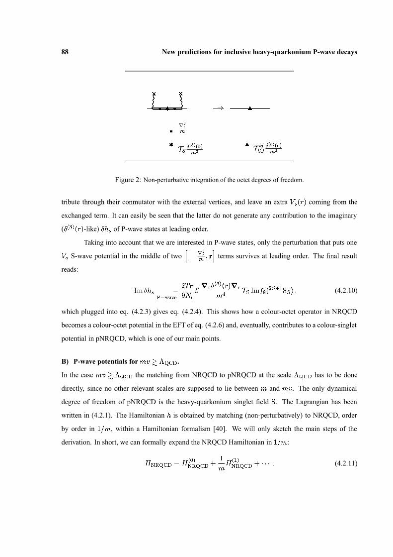
88 New predictions for inclusive heavy-quarkonium P-wave decays
� � ��
� �
� � � � � � �� �
� ��� �
� ��
� �
� � � �� � �
� �
Figure 2: Non-perturbative integration of the octet degrees of freedom.
tribute through their conmutator with the external vertices, and leave an extra�
� � � � coming from the
exchanged term. It can easily be seen that the latter do not generate any contribution to the imaginary
( ��
� �� � � -like) � � � of P-wave states at leading order.
Taking into account that we are interested in P-wave states, only the perturbation that puts one� �
S-wave potential in the middle of two�
�� �
�� � �
� terms survives at leading order. The final result
reads:
��
� � �
���� �
� � � � �
�
�
� ��
��
� � � ��
� �� � � � �
� � � ��
� � � �� � � �
� � � � (4.2.10)
which plugged into eq. (4.2.3) gives eq. (4.2.4). This shows how a colour-octet operator in NRQCD
becomes a colour-octet potential in the EFT of eq. (4.2.6) and, eventually, contributes to a colour-singlet
potential in pNRQCD, which is one of our main points.
B) P-wave potentials for � � �� � � �� .
In the case � � �� � � �� the matching from NRQCD to pNRQCD at the scale � � �
� has to be done
directly, since no other relevant scales are supposed to lie between � and � � . The only dynamical
degree of freedom of pNRQCD is the heavy-quarkonium singlet field � . The Lagrangian has been
written in (4.2.1). The Hamiltonian � is obtained by matching (non-perturbatively) to NRQCD, order
by order in� � � , within a Hamiltonian formalism [40]. We will only sketch the main steps of the
derivation. In short, we can formally expand the NRQCD Hamiltonian in� � � :
� �� �
� � �
� � � �� �
� ��
��
� � � �� �
� � � � � � (4.2.11)
4.2 Computation 89
The eigenstates of the heavy-quark-antiquark sector can be labelled as:
� �� � � � � � � � � �
� � � � � � ��
� ��
�
�� �
� � � � � � �� � �
� � � � �
where � labels the colour-related degrees of freedom (spin labels are not explicitly displayed for sim-
plicity). Assuming a mass gap of � � � � �� � much larger than � �
� , all the excitations ( � ���) decouple
and the ground state ( � ��) corresponds to the singlet state. Therefore, the matching condition reads:
��
� � � � � � � � ��
� ��
� � ��� � � � � � � � � � � �
� � � �� � � �
�� �
� � � � ��
� � �
�� �
� � � � ��� � � (4.2.12)
Up to � ��
� ��
� the imaginary contributions are only carried by the Wilson coefficients of the dimension
6 and 8 four-heavy-fermion operators in NRQCD. Since we are only interested in eq. (4.2.3) a huge
simplification occurs and only two contributions survive. From the dimension 8 operators we obtain:
��
� � �
�� �
� � � � ��
� � �
�� �
� � � � ��� � �
�
� �
��
�� �
��
� � � � � � � �
�� �
� �� �
� ��
� ��
� � ��� �
�� �
���� �
� � � � �
� (4.2.13)
�
�� � �
�
� �
�� � � �
� �� � �
� � � � � ��
� �� � � �
� �� � �
�� �
� � � � ��
� � �
�� �
� � � � ��� � �
On the other hand, we also have contributions from the iteration of lower-order�
� � corrections to
the NRQCD Hamiltonian with the dimension 6 four-heavy-fermion operators. The only term that con-
tributes to eq. (4.2.3) is:
��
� � �
�� �
� � � � ��
� � �
�� �
� � � � ��� � �
�
� �
��
� � ��
�� � � � � � � �
�� � �
� �� �
�� �
�� � �
�� �
� � ����� �
� � � � �
� (4.2.14)
The explicit computation of the right-hand side of eq. (4.2.14) gives (as far as the P-wave
contribution is concerned) eq. (4.2.7). Therefore, the sum of the contributions from eqs. (4.2.13) and
(4.2.14) coincides with eq. (4.2.3), after the replacements (4.2.4) and (4.2.5).
We can now obtain the decay widths by using eq. (4.2.3). At first order in QMPT, we obtain:
�� �
�
� � � ��
� �� �
� �� �
��
�
�� � � �
� �� � � � � �
�� �
� ��
��
� � � �� �
� �� � �
� � � ��� � � �
�� �
�
� � � (4.2.15)
where: ��
� � � ��
��
� � � � � ��
� , ��� � � �
��
�� � � � �
�� ( � � � � � ), � is the principal quantum number,
and � � � � � � � the radial wave function at leading order. Comparing with the standard NRQCD formula,
where spin symmetry has already been used, we have:
� � � � ��
� � � � ��
� � � � � � � ��
� � � � � �� �
�� � � �
�� �
�
� ��
� � � � � �� � � � (4.2.16)
90 New predictions for inclusive heavy-quarkonium P-wave decays
The information gained with this formula is that all non-perturbative flavour and principal quan-
tum number dependence is encoded in the wave function, as in the colour-singlet operators. The addi-
tional non-perturbative parameter�
� � � is universal: it only depends on the light degrees of freedom of
QCD. This implies that the following relation between decay widths is also universal:
�� � � � �
�
�
���� �
� � � � �� �
� � �� � �
�� �
� �� � � � �
�� �
� �� �
� � � � �� � � � � �
� � � �
�� �
�� � � �
�� �
� ��� � � � � � �
� � � � � �
�� � � �
� � � � ��
� �� �
� �� � � � � � � � � � � � � � �
�� � �
� � � ��
� �� �
�� (4.2.17)
It is interesting to notice that the UV behaviour of�
has the logarithmic divergence:
�� � � � � �
�� � � � �
�
��
� � (4.2.18)
which matches exactly the IR log of the � � � � � correction of� � � � �
� �� � �
� � , and hence the cancellation
originally observed in [76] is fulfilled. Then one could consider the LL RG improvement of�
by using
the results of ref. [77] for the running of the octet-matrix element. One obtains ( � � �� � � �
� � � �� � �
� ):
�� � � �
�� �
�
� �
��
�� � �
� �
��
� � � ��
�
� � � � �� (4.2.19)
4.3 Applications
Let us apply the above results to actual quarkonium, under the assumption that our framework,
discussed in the paragraph before eq. (4.2.1), provides a reasonable description for the P-wave states ob-
served in nature. The numerical extraction of�
is a delicate task, since several of the Wilson coefficients
(see Ref. [80] for a full list of them) have large next-to-leading order contributions, which may spoil
the convergence of the perturbative series. This problem is not specific of our formalism, but belongs
to the standard formulation of NRQCD. Here, in order to give an estimate, it is only used those data
that provide more stable results in going from the leading to the next-to-leading order, more precisely
the average of eq. (4.2.17) for ��
��
� � ��
��
� , �� �
�� �
� � ��
��
� , and ��
��
� � ��
��
� , �� �
�� �
� � ��
��
� .
The experimental data have been taken from [81] and updated accordingly to [82, 83]. The final value
reads:
��
� � � � � ��
� ��
� �
�
� � � � (exp) � (4.3.1)
where we have used the NLO results for the Wilson coefficients with a LL improvement. The errors
only refer to the experimental uncertainties on the decay widths. Theoretical uncertainties mainly come
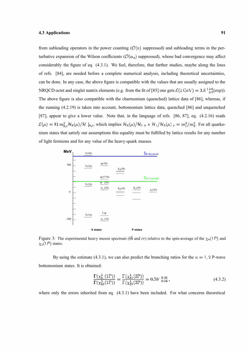
4.3 Applications 91
from subleading operators in the power counting ( � � � � suppressed) and subleading terms in the per-
turbative expansion of the Wilson coefficients ( � � � � � suppressed), whose bad convergence may affect
considerably the figure of eq. (4.3.1). We feel, therefore, that further studies, maybe along the lines
of refs. [84], are needed before a complete numerical analysis, including theoretical uncertainties,
can be done. In any case, the above figure is compatible with the values that are usually assigned to the
NRQCD octet and singlet matrix elements (e.g. from the fit of [85] one gets�
�� �
� � � � � �
� �� � �
� � � � (exp)).
The above figure is also compatible with the charmonium (quenched) lattice data of [86], whereas, if
the running (4.2.19) is taken into account, bottomonium lattice data, quenched [86] and unquenched
[87], appear to give a lower value. Note that, in the language of refs. [86, 87], eq. (4.2.16) reads�
� � � �� �
��
� � � � � � � � � � � � � � � , which implies � � � � � � � � � � � � � � � � � � � � � � ��� � �
�
� . For all quarko-
nium states that satisfy our assumptions this equality must be fulfilled by lattice results for any number
of light fermions and for any value of the heavy-quark masses.
S states P states
J
Υ(4S)
Υ(3S)
Υ(2S)
Υ(1S)
(3S)ψ
/Ψ
Χ
Χ Χhc
(2P)
(1P)
b
b(1P)c (1P)c
η c (1S)
η (2S)
(3770)ψ
−500
500
0
(2S)ψ
BB threshold
DD threshold
MeV
Figure 3: The experimental heavy meson spectrum ( � � � and � �� ) relative to the spin-average of the � � �� �
� and� � �
� �� states.
By using the estimate (4.3.1), we can also predict the branching ratios for the � ��
��
P-wave
bottomonium states. It is obtained:�
� ��
� � �� �
� ��
� ��
� � �� �
� ��
�� �
�� � �
� �� �
�� �
�� � �
� �� �
��
�
� � � � � � �
� � � � � � (4.3.2)
where only the errors inherited from eq. (4.3.1) have been included. For what concerns theoretical
92 New predictions for inclusive heavy-quarkonium P-wave decays
uncertainties, the comments after eq. (4.3.1) apply also here (with a better behaviour of the perturbative
series). Note that the first equality holds independently from eq. (4.3.1) and from the use of charmonium
data and, hence, provides a more robust prediction. The remaining branching ratios can be obtained
using spin symmetry. Notice also that, although no model-independent predictions can be made for the
decay widths (they depend on the wave function at the origin, which is flavour and state dependent),
our results allow any model that gives a definite value to ��
� � � ��
� to make definite predictions.
In conclusion, we have exploited the fact that NRQCD still contains irrelevant degrees of free-
dom for certain heavy quarkonium states, which can be integrated out in order to constrain the form
of the matrix elements of colour-octet operators. We have focused on the operators relevant to P-wave
decays, which allowed us to produce concrete, new, rigorous results. However, it should be clear from
the structure of the pNRQCD Lagrangian itself, that similar results can be obtained for matrix elements
of any colour-octet operator.
Conclusion
In the previous pages we have offered a brief account on some facets of non-relativistic ef-
fective field theories, as seen through present concern calculations. From the accurate computation
of pionium’s lifetime, a low energy observable sensitive to a high energy QCD parameter such as the
quark condensate, to P-wave quarkonia hadronic decays, going through the display of analytic expres-
sions for the corrections induced by light fermion finite mass effects, or the problem of renormalizing
the nucleon-nucleon interaction, every chapter constitutes a well-defined problem whose solution goes,
inextricably, tied up to a NREFT of its own. So, while in the first chapter, we were compelled to de-
rive a low energy version of the Chiral Lagrangian( ��
), well-suited to tackle with pionium, the second
chapter introduced the non-relativistic offsprings of QED and QCD and, in the third one, pions were
integrated from the two nucleon sector of the ��
.
All results extracted can be quickly summarized in the following lines:
� Concerning pionium’s lifetime calculation, we performed a step-by-step construction of the dif-
ferent Lagrangians that appear all the way down from the ��
to our ��
� ��
, that is the right
theory to address the problem at hand. We kept track of all the terms that are needed in or-
der to achieve the expected accuracy aimed by the DIRAC’s experiment (10%) and our final
formula (1.7.3) is exhibited in the most convenient form. That is, all corrections coming from
the quantum mechanical calculation are shown explicitly, whereas the ones that enter through the
matching with Chiral Perturbation Theory ( � � � ) are resummed in the � � � � term. That provides
a very general (and pedagogical) framework where the power and simplicity of non-relativistic
techniques is best grasped. It is worth emphasizing that only such a computation is capable of
delivering a result where systematicity allows for a straightforward implementation and accuracy
94 Conclusion
is always under control.
� In the chapter devoted to light fermion finite mass effects the results (2.2.1) and (2.3.1) consti-
tute analytical expressions that apply to a large range of different systems among which we find
hadronic atoms (see Tables II and III), as well as quarkonia (see Table IV). Given their impor-
tance, those corrections are of current interest, as we learn from the section on Related works.
� The third chapter, which starts with a fairly large historical introduction to the subject of renor-
malization in the context of nucleon-nucleon interaction, offers a rigorous approach to the prob-
lem from a purely theoretical point of view. That allows us to draw very definite conclusions on
the nature of the solution, besides signalling those lines that should be pursued in order to define
a consistent effective field theory out of such a nuclear issue. So, what we get is that the tradi-
tional OPEP (One Pion Exchange Potential) in the � �� - �
�� channel, which is iterated through a
Lippmann-Schwinger equation, cannot be renormalized unless we allow the constant accompa-
nying a non local potential (the tensor term) to flow. What is worst, is this case the amplitude
lacks from partial wave mixing. So, we expect that this tensor interaction should be treated per-
turbatively. We show that, up to first order in perturbation theory, that defines a renormalizable
potential and get the flows that prove this (see eqs. (3.4.1.5), (3.4.1.10), (3.4.2.9) and (3.3.11)).
� The last part of the work concerns the inclusive hadronic decay of P-wave quarkonia. After
realising that NRQCD is still a too general theory for actual states, we integrate the potential one
in both the perturbative ( � ��
� � � � � � � � ) and non perturbative ( � � � � �
� � ) situations.
What we get, expressions (4.2.3) and (4.2.4), is that the former colour-octet matrix elements in
NRQCD, can be rewritten in terms of the derivative of the singlet P-wave wavefunction at the
origin and additional universal constants (4.2.5). The latter also absorve infrared divergences
encountered in the singlet coefficients. In all, we are able to produce new relations (4.2.17) and
give some predictions (4.3.1) that relate the branching ratios of hadronic decays of systems with
different heavy flavour and different principal quantum number.

Resumen
Sistemas no relativistas
En esta tesis hemos tratado fundamentalmente de transmitir parte del espıritu que anima a las
teorıas efectivas no relativistas (NREFTs). Mediante una serie de calculos recientes y variados, basa-
dos en su filosofıa, se ha demostrado que existe un gran campo de aplicabilidad de su potencial entre
aquellos sistemas ligados cuya velocidad relativa � constituye un adecuado parametro de expansion. A
traves de los diferentes capıtulos, que tratan a la vez de emfatizar los aspectos teoricos mas destacables
en el desarrollo del calculo, distintos atomos hadronicos regidos por la jerarquıa ��
� �
�� �
�
han merecido nuestra atencion.
De hecho en la naturaleza existen varios sistemas de partıculas ligados para los que se verifica
esta condicion. Ejemplos tıpicos en el dominio de las interacciones electromagneticas son el positro-
nium ( ��
� � ) y el muonium ( � � ��
). Sus analogos en el mundo de las interacciones fuertes son los
estados de heavy quarkonia ( � � , � � , � � , � � ). Entre unos y otros encontramos a sistemas tales como los
atomos hidrogenoides y el pionium ( ��
� � ). En su tratamiento se dan problemas tecnicos comunes
a cualquier calculo de un estado ligado no relativista, aun y cuando nos hallemos en una situacion
puramente perturbativa. Complicaciones adicionales surgen en el contexto de una teorıa fuertemente
acoplada, como es el caso de QCD.
Tradicionalmente se habıan empleado ecuaciones de Bethe-Salpeter (relativistas) en la res-
olucion del espectro de estados ligados. No obstante, este precedimiento, que resulta en todo adecuado
para el calculo de amplitudes de scattering, no es eficaz a la hora de hallar energıas de ligadura. La
razon estriba en el hecho de que las funciones de onda iniciales y finales son, en este ultimo caso, las

96 Resumen
interactuantes y, por lo tanto, no resulta trivial la seleccion del conjunto de diagramas que intervienen a
un orden determinado en la constante de acoplamiento. Esto es, la contribucion de cada diagrama no se
deriva directamente del numero de vertices de este. Por ejemplo, es bien sabido que en el positronium
es preciso resumar la infinita serie de fotones potenciales, ya que todos ellos intervienen al mismo orden
en � .
El problema es, en su raız, que se esta obviando la naturaleza inherentemente no relativista del
problema, y la consiguiente existencia de tres escalas fısicas vinculadas: � , la masa de las partıculas;
� � � � , que es el momento relativo del estado; y � � � �� o energıa de ligadura. Todas ellas
aparecen enlazadas en cualquier diagrama de Feynman.
Otras maneras de atacar el problema de estos estados ligados, reducciones no relativistas esen-
cialmente, carecen de sistematicidad y de un mecanismo de control sobre las correcciones relativistas.
Problemas emergentes como la incorporacion de los efectos no potenciales, la cancelacion de las diver-
gencias ultravioletas en el calculo mecanico-cuantico o la carencia de criterios para incluir los distintos
terminos, ya sea perturbativa o no perturbativamente, se vieron solventados tras la aparicion de las
NREFTs.
Estas establecieron un puente de conexion entre la teorıa de campos y la mecanica cuantica.
Como toda teorıa efectiva, su punto de partida es la construccion, a partir de una teorıa mas general
(fısica de altas energıas), de una serie de tecnicas que permitan abordar calculos referidos a una escala
mas restringida (experimentos a baja energıa). El nexo comun a todas ellas es, pues, el hacer del
momento relativo del estado ligado, una de estas escalas de baja energıa cuya dinamica se pretende
describir, e integrar la informacion procedente de aquellos modos que no podemos excitar, � � , en
unos pocos coeficientes ordenados en potencias crecientes de �� .
Los ingredientes basicos para construir una EFT son:
� Las simetrıas que debe obedecer la teorıa de bajas energıas. Nos permitiran construir un La-
grangiano cuyos operadores se hallaran acordemente organizados en base al analisis dimensional
especıfico de nuestro problema. Como la precision con que se desea describir la fısica de bajas
energıas es conocida de antemano, la expansion de Lagrangiano en la/s escala/s de alta energıa
se truncara siempre al orden que nos interese.
� Este mismo analisis dimensional nos permite prefijar si un determinado operador es irrelevante,
Resumen 97
relevante o marginal para nuestra fısica.
� El matching permite relacionar los parametros de ambas teorıas. Este consiste en imponer que
diferentes funciones de Green off shell sean equivalentes a aquellas calculadas en la teorıa de
altas energıas. Procedimientos analogos son la integracion de los grados de libertad irrelevantes
o las transformaciones de Foldy-Wouthysen para la eliminacion de antipartıculas.
� Un procedimiento de regularizacion de las divergencias que surgen al calcular las correcciones
cuanticas, ası como un esquema de renormalizacion.
El hecho de que nos refiramos en el primer punto al analisis particular de nuestro sistema ligado,
viene dado por el hecho que, atendiendo a los valores de las masas y al numero de fermiones pesados
de que este conste, nos hallaremos en distintas situaciones y, por lo tanto, precisaremos de diferentes
NREFTs. Esto es:
� Un partıcula pesada y otras ligeras (relativistas). La masa de la partıcula pesada ( � ) es mucho
mayor que las escalas tıpicas de las ligeras, y su inverso constituye el parametro de expansion de
la teorıa efectiva. Como estas ultimas son relativistas, obedecen una relacion de dispersion lineal
( � � � � � ). En definitiva, se verifica:
��
� � � � � � (.1)
En el caso de QCD, estas dos ultimas escalas son, ademas � � � � � . La teorıa efectiva disenada
a su proposito es HQET (heavy quark effective theory). En ella, la integracion de la escala � ,
puede ser realizada perturbativamente en � � � � � . A bajas energıas rige una simetrıa aproximada
de spin-flavour que le presta poder predictivo. Por todo ello, los calculos aparecen organizados
en una doble expansion en � � � � � y�
� ��
� . Para evaluar el tamano de un termino dado del
Lagrangiano se asigna, pues, la escala � � � � a cada potencia con dimensiones de energıa.
� Dos partıculas pesadas. En este caso tenemos:
� � � � ��
� � ��
� � (.2)
La escala � � � � � � se denomina hard, la escala � � � recibe el nombre de soft y � constituye la
escala ultrasoft. Dentro de este apartado se puede distinguir entre:
98 Resumen
– � ��
� � . Es el caso de los atomos hidrogenoides o del sistema�
� , aunque en este
ultimo caso de manera ya no tan clara. La partıcula mas pesada se toma como estatica
(negligiendose su termino cinetico) y la otra como no relativista.
– � �� � � . En esta situacion se encuentran el positronium, muonium, � � , entre otros.
Ambas partıculas deben ser consideradas como no relativistas.
Respecto a QCD, la primera NREFT creada fue NRQCD (non-relativistic QCD). Factorizaba la
escala � sin preocuparse por la jerarquıa adicional � ��
� � � . Con la presencia adicional de
� � � � , tres escalas permanecıan indeterminadas, con lo consiguiente falta de un contaje unıvoco
mas alla de primer orden. Su problema radica, por lo tanto, en que no resulta explıcito en modo
alguno la dominancia del regimen potencial de la interaccion (esto es, del potencial Coulombiano
estatico en la situacion perturbativa). pNRQCD (potential NRQCD) es la teorıa que se ocupa de
ello. Proviene de integrar en NRQCD los grados de libertad soft. Ello fija dos cutoff ultravioleta:
� � y � � . El primero satisface � � �� � � � � � y es el cutoff de la energıa de los quarks y
de la energıa y momento de los gluones. El segundo verifica � � � � � � � y es el cutoff del
momento relativo del sistema ligado.
Mientras que el matching entre QCD y NRQCD es perturbativo en � � � � � , el matching entre
NRQCD y pNRQCD puede ( � ��
� � � � ) o no ( � � � � � � ) serlo, en funcion del sistema
que nos ocupe. En cualquier caso, la integracion de la escala � � produce, como coeficientes
de matching en pNRQCD, terminos potenciales. En general estos dependeran de la escala de
matching. Esta funcionalidad es cancelada en el espectro por la contribucion de los gluones
ultrasoft.
Aspectos tratados
Empezamos por el pionium, sistema formado por �
y , ligado electromagneticamente y
que decae por interaccion fuerte, para dedicar al calculo de su vida media el primer capıtulo. Este
nos sirvio como perfecto ejemplo de como la integracion de diferentes escalas de momento/energıa no
dinamicas, mediante la tecnica de matching, nos conduce de una teorıa efectiva de baja energıa a otra
subyacente y simplificada, en la que la informacion de mas altas energıas relevante para acometer el

Resumen 99
problema que nos ocupa queda condensada en unos pocos parametros. En este ejemplo en concreto
se requerıa que estas constantes fueran calculadas explıcitamente, estableciendo la equivalencia entre
amplitudes de scattering calculadas en una teorıa a energıas intermedias, tal como Chiral Perturbation
Theory ( � PT) y nuestra teorıa efectiva no relativista cuyo unico grado de libertad era el estado ligado.
Pero solo porque unicamente ası podıamos aislar uno de estos coeficientes, el llamado condensado de
quarks, responsable de la rotura de la simetrıa quiral de QCD, y cuyo valor, pobremente determinado,
nos interesaba. No obstante, tal como se desarrollo el calculo, esta necesidad queda relegada a las
ultimas secciones, con lo que se pretende dar relevancia al hecho de que cuanto se esta haciendo es
reflejo de un procedimiento totalmente general y que, por lo que respecta a la vida media del estado,
bien se podrıa dejar estos coeficientes como parametros a determinar, ya sea por simulacion, ya ex-
perimentalmente. Otros puntos sobre los que se debatio fueron el papel fundamental de las simetrıas
obedecidas por la teorıa de bajas energıas a la hora de construir el correspondiente Lagrangiano, la in-
variancia Lorenz, la posibilidad de reparametrizar los campos, como la observancia del power counting
selecciona unicamente los terminos que seran precisos posteriormente en vistas a ofrecer resultados
consistentes, de error acotado y prefijado, ...
Por lo que atane a la parte mas tecnica, hemos desarrollado un metodo que permite obtener el propa-
gador Coulombiano�
� � � � � � � � en Regularizacion Dimensional (DR). Dado que los coeficientes de
nuestra ultima teorıa de bajas energıas se derivan de � � � , donde los calculos son realizados en DR, es
imprescindible que todos las expresiones sean ofrecidas en este esquema, para mayor eficacia.
El segundo capıtulo constituyo tambien un ejemplo de calculo estandar dentro de una teorıa
efectiva no relativista. Hablamos de los efectos de masa finita de los grados de libertad ligeros, a traves
de la correccion por polarizacion del vacıo, sobre la energıa de ligadura y la funcion de onda en el
origen de estados debilmente ligados. Las correspondientes NREFTs aportan los conceptos precisos
para entender porque estos no pueden ser negligidos (importancia relativa de las escalas integradas),
nos fijan como deben tratarse escalas de similar magnitud que desean ser integradas, y flexibilizan que
un mismo calculo sea susceptible de aplicacion a multitud de sistemas, cuya dinamica es, o puede ser,
en gran medida diferente. Ası pues, nuestras Tablas II, III y IV se refieren, respectivamente, a atomos
hadronicos y heavy quarkonia. Todas estas correcciones han sido halladas aplicando las expresiones
analıticas (2.2.1) y (2.3.1), que ofrecemos por vez primera en la literatura.
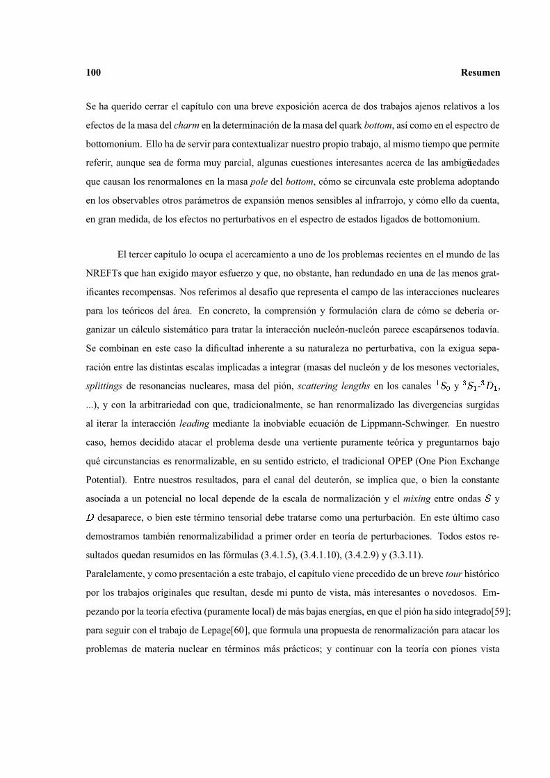
100 Resumen
Se ha querido cerrar el capıtulo con una breve exposicion acerca de dos trabajos ajenos relativos a los
efectos de la masa del charm en la determinacion de la masa del quark bottom, ası como en el espectro de
bottomonium. Ello ha de servir para contextualizar nuestro propio trabajo, al mismo tiempo que permite
referir, aunque sea de forma muy parcial, algunas cuestiones interesantes acerca de las ambig �
�
edades
que causan los renormalones en la masa pole del bottom, como se circunvala este problema adoptando
en los observables otros parametros de expansion menos sensibles al infrarrojo, y como ello da cuenta,
en gran medida, de los efectos no perturbativos en el espectro de estados ligados de bottomonium.
El tercer capıtulo lo ocupa el acercamiento a uno de los problemas recientes en el mundo de las
NREFTs que han exigido mayor esfuerzo y que, no obstante, han redundado en una de las menos grat-
ificantes recompensas. Nos referimos al desafıo que representa el campo de las interacciones nucleares
para los teoricos del area. En concreto, la comprension y formulacion clara de como se deberıa or-
ganizar un calculo sistematico para tratar la interaccion nucleon-nucleon parece escaparsenos todavıa.
Se combinan en este caso la dificultad inherente a su naturaleza no perturbativa, con la exigua sepa-
racion entre las distintas escalas implicadas a integrar (masas del nucleon y de los mesones vectoriales,
splittings de resonancias nucleares, masa del pion, scattering lengths en los canales � �� y � �
� - �
�� ,
...), y con la arbitrariedad con que, tradicionalmente, se han renormalizado las divergencias surgidas
al iterar la interaccion leading mediante la inobviable ecuacion de Lippmann-Schwinger. En nuestro
caso, hemos decidido atacar el problema desde una vertiente puramente teorica y preguntarnos bajo
que circunstancias es renormalizable, en su sentido estricto, el tradicional OPEP (One Pion Exchange
Potential). Entre nuestros resultados, para el canal del deuteron, se implica que, o bien la constante
asociada a un potencial no local depende de la escala de normalizacion y el mixing entre ondas�
y
�desaparece, o bien este termino tensorial debe tratarse como una perturbacion. En este ultimo caso
demostramos tambien renormalizabilidad a primer order en teorıa de perturbaciones. Todos estos re-
sultados quedan resumidos en las formulas (3.4.1.5), (3.4.1.10), (3.4.2.9) y (3.3.11).
Paralelamente, y como presentacion a este trabajo, el capıtulo viene precedido de un breve tour historico
por los trabajos originales que resultan, desde mi punto de vista, mas interesantes o novedosos. Em-
pezando por la teorıa efectiva (puramente local) de mas bajas energıas, en que el pion ha sido integrado[59];
para seguir con el trabajo de Lepage[60], que formula una propuesta de renormalizacion para atacar los
problemas de materia nuclear en terminos mas practicos; y continuar con la teorıa con piones vista

Resumen 101
a traves de distintos power countings[63, 64], donde queda perfectamente ilustrada la inextricabilidad
entre el problema de contaje y la renormalizabilidad; acabamos esbozando algunos acercamientos alter-
nativos mas recientes[67, 68] de los cuales pormenorizamos las dificultades existentes en la Discusion
del capıtulo y en el Apendice H.
Finalmente, el ultimo capıtulo ha sido dedicado a analizar los decaimientos hadronicos de los
estados en onda P de quarkonium. Se ha visto que, siempre que se puede integrar en NRQCD la escala
soft � � , se alcanza una nueva teorıa, que contiene unicamente grados de libertad ultrasoft y que es
mas restrictiva. Ello, a la vez que da lugar a nuevas relaciones entre procesos en que decaen sistemas
con diferente flavour, nos permite escribir aquellos preteritos elementos de matriz de NRQCD que
eran octetes de color, en terminos de derivadas de la funcion de onda en el origen del estado singlete
observable, y de constantes universales adicionales que son susceptibles de ser calculadas en el lattice.
Los calculos han sido realizados tanto en la situacion perturbativa, esto es � ��
� � � � � � � � , como
en la no perturbativa, � � � � ��
� � . Las nuevas relaciones y predicciones se resumen en las expresiones
(4.2.17) y (4.3.1).

Appendix A
The DIRAC experiment
DIRAC (Dimeson Relativistic Atom Complex) experiment[88], aimed to determine the dif-
ference of scattering lengths � ��� � � �� � with 5% accuracy by measuring the lifetime of pionium[88],
will provide us, as discussed in Chapter 1, with evidence in favour or against the existence of a large
quark-antiquark condensate in QCD’s vacuum. Last available experimental data[89] for the isospin zero
scattering length, � �� � �
� � ��
� �, is certainly poorly determined for such a purpose.
A.1 Experimental method
To form atomic �
�� � bound states, pions must have a small relative momentum in the center of
mass (CM) rest frame ( ��
MeV.) and must be found closer than the Bohr radius (387 fm.). Such pions
originate from short-living sources, such as the � and � mesons or the � baryon resonances, and not
from the long-living ones ( � and � �� ). So, pionium production is proportional to the double inclusive
cross section� � ��
� � � � � of ��
and � � pairs from short-living sources without Coulomb interaction in the
final state, and to the squared atomic wave function of �
�-states at the origin � � � � � � �
� :
� � ��� � �
� �
� �� � �
� �
� � � � � � �� � � ��
� � � � �
� � � �� � �
� �
�� (A.1.1)
where � � , � � and � � are momentum, energy and mass of the pionium atom in the laboratory system.
After being produced by hadronic interaction, relativistic pionium atoms (2 GeV. � � � � 6
GeV.) move in the target. Then, they decay or, due to the electromagnetic interaction with the target
material, get excited or ionized. The break-up process is easy to track, as it creates characteristic
The DIRAC experiment 103
0
0.1
0.2
0.3
0.4
0.5
0.6
0.7
0 1 2 3 4 5 6 7 8 9 10τ 10-15 s
P brBe 2000 μmTi 263 μmNi 104 μmPt 22 μmp=4.7 GeV/c
Figure 1: Probability of pionium break-up in the target.
�
�� � atomic pairs with small CM relative momentum ( � 3 MeV.), small opening angle ( � � � .35
mrad. for � � =4.7 GeV.) and nearly identical energies in the laboratory system ( � �� � � at .3 %
level). Using atomic interaction cross sections, for a given material and thickness, one can calculate the
break-up probability for arbitrary values of pionium momentum and lifetime. In fig. 1 we show those
dependencies for the pionium momentum � =4.7 GeV.
Comparison of the measured break-up probability � ��
�
� �
� � (ratio of broken-ups � � over�
�produced pionium atoms) with the calculated dependence of � �
� on � gives the value of the lifetime.
The measurement of broken-up � � pionium atoms is performed through the analysis of the
experimental distribution in relative momenta (Q) of �
�� � pairs. The free pion pair distribution can be
written as the sum of the non-Coulomb (nC) and the Coulomb (C) pair distributions:
��
� �
� �� � �
��
� �
� � � ��
�
� � �
��
� �
� � ��
�
��
�� � �
� � �
�� � � �
��
�
� � ��
� � ��
� � � � �� � � � � � (A.1.2)
where�
� � � � is the Coulomb and �� � � � � the strong correlation factors. Here it is assumed that
the non-Coulomb distribution of ��
- � � pairs can be extracted from the experimental distribution of
accidental pairs�
� � � . Then the free pion pair distribution is given by:
��
� �
� �� � �
��
� �
� � � ��
�
� � ��
��
� � � � �� � � � �
� � � � � � � (A.1.3)
where�
� , and � are free parameters. In the region Q � 3 MeV. there are mainly free pairs. After
fitting this part of the distribution with the function (A.1.3), the extrapolation of the function to the
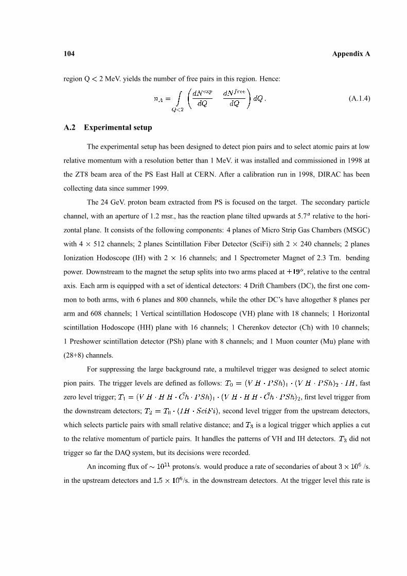
104 Appendix A
region Q � 2 MeV. yields the number of free pairs in this region. Hence:
� � �
�� �
�
� ��
��
�
� � ��
�
� �
� �
� �� � � � (A.1.4)
A.2 Experimental setup
The experimental setup has been designed to detect pion pairs and to select atomic pairs at low
relative momentum with a resolution better than 1 MeV. it was installed and commissioned in 1998 at
the ZT8 beam area of the PS East Hall at CERN. After a calibration run in 1998, DIRAC has been
collecting data since summer 1999.
The 24 GeV. proton beam extracted from PS is focused on the target. The secondary particle
channel, with an aperture of 1.2 msr., has the reaction plane tilted upwards at 5.7�
relative to the hori-
zontal plane. It consists of the following components: 4 planes of Micro Strip Gas Chambers (MSGC)
with 4 � 512 channels; 2 planes Scintillation Fiber Detector (SciFi) sith 2 � 240 channels; 2 planes
Ionization Hodoscope (IH) with 2 � 16 channels; and 1 Spectrometer Magnet of 2.3 Tm. bending
power. Downstream to the magnet the setup splits into two arms placed at� � �
�
, relative to the central
axis. Each arm is equipped with a set of identical detectors: 4 Drift Chambers (DC), the first one com-
mon to both arms, with 6 planes and 800 channels, while the other DC’s have altogether 8 planes per
arm and 608 channels; 1 Vertical scintillation Hodoscope (VH) plane with 18 channels; 1 Horizontal
scintillation Hodoscope (HH) plane with 16 channels; 1 Cherenkov detector (Ch) with 10 channels;
1 Preshower scintillation detector (PSh) plane with 8 channels; and 1 Muon counter (Mu) plane with
(28+8) channels.
For suppressing the large background rate, a multilevel trigger was designed to select atomic
pion pairs. The trigger levels are defined as follows: � � � ��
� � � � � � � � ��
� � � � � � � � � � , fast
zero level trigger; � � � ��
� � � � ��� � � � � � � � � �
�� � � � �
�� � � � � � � � , first level trigger from
the downstream detectors; � � � � � � � � � �
�� � � � � , second level trigger from the upstream detectors,
which selects particle pairs with small relative distance; and � � is a logical trigger which applies a cut
to the relative momentum of particle pairs. It handles the patterns of VH and IH detectors. � � did not
trigger so far the DAQ system, but its decisions were recorded.
An incoming flux of �� � � protons/s. would produce a rate of secondaries of about � �
� �/s.
in the upstream detectors and� � �
�� �
/s. in the downstream detectors. At the trigger level this rate is
The DIRAC experiment 105
Figure 2: Experimental setup
reduced to about�
�
� � � /s., with an average event size of about .75 Kbytes.
With the 95 � m. thin Ni target, the expected average pionium yield, within the setup acceptance,
is � �
��
� �� � /s., equivalent to a total number of �
� � � � protons on target in order to produce one
pionium atom.
A.3 First experimental results
The data taking has been done mainly with ��
� � and � � � pairs and also ��
� � pairs for detector
calibration. For the first data analysis only the most simple events were selected and processed, that
is, those with a single track in each arm and signals in DC, VH and HH. The tracks in the DC’s were
extrapolated to the target plane crossing point of the proton beam. A cut was applied along X and Y
distances between the extrapolated track and the hit fiber of the SciFi planes (18 mm. divided by the
particle momentum in GeV., to take into account the multiple scattering effect). Finally, these events
were interpreted as ��
� � or � � � pairs produced in the target.
The difference in the time-of-flight � � between the positive particle (left arm) and negative
particle (right arm) of the pair at the level of VH is presented in fig. 3.
The first interval -20 � � �� -.5 ns. corresponds to accidental hadron pairs (mainly �
�� � ). In
the second interval -.5 � � �� .5 ns. one observes the peak of coincidence hits associated to correlated
hadron pairs over the background of accidental pairs. The width of the correlated pair peak yields the
time resolution of the VH ( � � � 250 ps.). The asymmetry on the right side of the peak is due to the
106 Appendix A
0500
10001500200025003000
-20 -15 -10 -5 0 5 10 15 20Δt (ns)
Num
ber
of E
vent
s
N1
N2
N3 N4
σt=255 ps
Figure 3: VH time-of-flight difference distri-bution for pair events
Figure 4: Positive particlemomentum versus VH time-of-flight difference for particlepairs
admixture of protons in the �
�sample, that is, � � � events. Hence the third interval .5 � �
�� 20 ns.
contains both accidental pairs and � � � events.
This time-of-flight discrimination between ��
� � and � � � events is effective for momenta of
positive particles below 4.5 GeV. This is demonstrated in fig. 4, where the scatter plot of positive particle
momentum versus difference in time-of-flight �� in VH is shown. The single particle momentum
interval accepted by the spectrometer is 1.3 � 7 GeV.
For correlated ��
� � pairs, Coulomb interaction in the final state has to be considered, because
it increases noticeably the yield of ��
� � pairs with low relative momentum in CM (Q � 5 MeV.). For
accidental pairs this enhancement is absent.
Fig. 5 shows the distribution of the longitudinal components � � (the projection of Q along the
total momentum of the pair) for correlated pairs. There are plotted pair events with positive particle
momentum � � � � � 4.5 GeV., occurring within the correlated �� peak and with transversal component
� � � 4 MeV. to increase the fraction of low relative momentum pairs.
In the region � � � ��
10 MeV. there is a noticeable enhancement of correlated ��
� � pairs due
to Coulomb attraction in the final state.
The most important parameter for data analysis is the resolution in � � and � � . This has been
measured by the reconstruction of the invariant mass of � � � pairs. The distribution of � � � invariant
mass is presented in fig. 6. Positive particles are restricted to momenta larger than 3 GeV., and the time-

The DIRAC experiment 107
Figure 5: Correlated � � � � pairswith positive particle momenta
� � � �� � � �
GeV/c and � � � �MeV/c.
Figure 6: �� � invariant mass for proton
momenta � � � � � 3 GeV.
of-flight must lie in .5 � ��
� 18 ns. A clear peak at the � mass � � = 1115.6 MeV. � with a standard
deviation � = 0.92 MeV. � can be seen. These mass parameter values show a good detector calibration
and coordinate detector alignment, with an accuracy in momentum reconstruction better than 0.5 % in
the kinematic range of � decay products. This gives for the relative momentum resolution �� � 2.7
MeV. For ��
� � pairs a better resolution can be obtained, due to the different kinematics.
108 Appendix A
The following table displays the breakup probability results so obtained until now:
� � � � � � � � � � � � � �� � � � ��
� � � � � � �
Pt-99 analysed 150�
35 250�
30 0.58�
0.16 0.81�
0.24 0.68�
0.01
(21 days)
Ni-00 analysed 1470�
140 4730�
130 0.31�
0.04 0.43�
0.05
(89 days)
Ti-00 analysed 710�
100 2010�
85 0.29�
0.04 0.49�
0.09
(31 days)
Ti-01 analysed 1120�
130 3820�
120 - 0.36�
0.05
(46 days)
Ni-01 progress 2120�
170 6630�
150 -�
0.04
(72 days)
Ni-01 expected 1330�
140 4150�
120 -�
0.04
(45 days)
Ni-00/01 all 4920�
140 15510�
230 -�
0.025 0.436�
0.022
(206 days)
Ti-00/01 all 1830�
160 5830�
150 - 0.39�
0.04 0.304�
0.017
(77 days)
Table X: Breakup probability results. The last two rows provide an an accuracy of � �� = 10%.
As for the lifetime value this means:� � ! # � � % #
� � � � �
� ( �� � � � � � � � � � � � * #
� � + �
�
� ��
�� � � �
� 2.8�
� � �
� � �
� �34 %
� � � �� � � �
��
� 5.4� � �
�
� � � �
�26 %
� ��
� � � � � 3.6� � �
�
�
� �
��
22 %
Note that the current error estimate is purely statistical. So far no systematic errors have been
proposed, in spite of the fact that they are expected to be quite significant.
Appendix B
Reparametrization invariance
Consider � � � � a relativistic spin zero field and its partition function:
��
�� �
�� � � � �
�� � � � � �
��
�� � � � � � � � � (B.1)
If�
is Lorentz invariant then:
��
�� �
��
� �� �
� �� � � �
�� � � � � � � (B.2)
In the non-relativistic regime we only need a subset of�
s which generate Green functions with the
external legs almost on shell. These may be chosen as:
�� � � � � �
� � � � � � � � �� � � � � � � � � � �
� � � � � � (B.3)
where � is the mass of � and�
� � � � is slowly varying (i.e. contains energy and momentum much
smaller than � ). From (B.2) and (B.3) one easily finds that for Lorentz transformations close to the
identity:
�� � � � � �
� �� � � � � � � � � � � � �
� � � � � � ��
� � � � � � � � (B.4)
In the non-relativistic regime�
��
� can be approximated to the desired order of accuracy by:
��
�� �
�� � �
�� �
� � � �
�� � � �
� � �
� � � � � � � � � � � ��
� � � � � � � �� � � � �
��� � � � � � � � � � � (B.5)
Then�
� � ��
� ��
� � must be invariant under the transformation (B.4). Invariance of the terms coupled
to the sources implies the following transformations for � � � � :
� � � � � � ��
� � � � � � � � � � � �
� � � � � � �� � � � � � � � (B.6)
110 Appendix B
Hence�
� � � � � ��
� must be constructed in such a way that it is invariant under (B.6). In order to do so,
notice first of all that � � � � � � does not transform in a way similar to � � � � . We would like to introduce a
kind of covariant derivative. The following operator appears to be a successful candidate:
� � � � � �� � � �
�
�� (B.7)
We have under Lorentz transformations:
� � � � � � � � � � � � � � �
�� � � �
� �
� � � � � �� �
��
�
� � � � � � � �� � � � (B.8)
which upon the change � � � � becomes:
� � � � � � � � � � � � ��
� � � �� �
� � � � � � (B.9)
Analogously, if we have � � � � � � � ��
� � � ��
� � � � � �� , � � � � � , we may define for � ��
�a
generalization of (B.7):
� � � � � �� � � ��
� �� (B.10)
Then � � � � � � � has the same transformation properties as � � � � � . We call � the weight of the composite
field � � � � � . If � ��
then � � � � � � � transforms as a usual Lorentz vector.
From the discussion above the following rules can be inferred in order to built a Lorentz invari-
ant non-relativistic effective theory for spin zero particles:
1. Write down all possible terms in the particle sector we are interested in with weight zero and no
derivatives up to the desired order.
2. For each term, which is not already of the higher relevant order, insert � s or � � s in all possible
ways. All � indices coming from the � � must be contracted in a Lorentz invariant way.
Applying the rules above we obtain the Lagrangians (1.3.3) and (1.3.4). Recall also that, for the
particular case we are interested in, the (minimal) suppression of � is � � � � whereas the (minimal)
suppression of � � is� � � � � .
Finally, let us mention that for practical purposes the rules that we have obtained are identical
to those derived from the so called reparametrization invariance [90] (see also [91]). Hence, it should

Reparametrization invariance 111
be clear that reparametrization invariance is nothing but a way to implement Lorentz symmetry in a
non-relativistic theory. We believe that this point is important and has not been sufficiently stressed in
the literature[92].

Appendix C
� �and
� �
� � � � � in (2.3.2) can be expressed in terms of Clausen integrals. We get:
� � � � � �
�����������������������������������������������������������
�
� � � ��
��
� ��
� � ��
� � � � ��
�
��
� ��
� � if � ��
� � �� � �
��
� � �� � �� � � � �
��
��
� ��
�if � �
�
� � � � � � � � � � � � ��
� � � � � � � ��
� � � � � � �� � � �
� � � � � � � � � � � � ��
� � � � � � � � ��
� � � � � �� � � �
� � ��
� � � �� � �
�� � � �
� � ��
� � � � � � � � ��
� � �� � �
�� � � � � � � � �
�� � �
�� � �
� � �� � � � �
� �
� �� � � �
��
��
��
� � ��
� �� �
� � � �
�� � �
�� � � � � � �
�� �
� � ��
� � � � � � � � ��
� �
�� � �
�� � � � � � � � �
�� �
� � ��
� � � � � � ��
� � if � ��
�
(C.1)
Recall that the Clausen integral is defined as:
� � � � � ��
� ��
�� �
� � � � � �
�
� � � � �� �
� ��
�� �
� �� � � � � � � � � � � � � � � � � �
� � (C.2)
� � � � � in (2.3.2) can be expressed in terms of dilogarithms. We get:
� � � � � �
�
� �� � �
�� � �
��
��
� � � � ���
� � � � �
��
��
� � � � ���
� � � � �
��
��
��
� � � � �� �
� � � �
� ��
��
� � � � �� � � � �
��
� � � � ���
� � � � �
��
� � � � ���
� � � � �
��
��
� � � � �� �

� � and � � 113
� � � �
� ��
� � � � �� � � � �
�� � � � �
��
� � � � �� � � � �
�� � � � �
��
� � � � �� �
�� � � � � � �
� � � ��
�� � � � �
��
� � � � �� � if � �
��
where �
�� � � � and �
��
� � �� �� .
� � ��
� ��
�� � � �
� � � � � �
�
� � � � ��
�� � �
��
��
� � � � � ��� �
� � � � �
��
��
� � � � � ��� �
� � � � �
��
�� �
��
� � � � � �� �
� � � �
� �� �
��
� � � � � �� � � � �
��
� � � � � ��� �
� � � � �
��
� � � � � ��� �
� � � � �
��
�� �
� � � � � �� �
� � � �
� �� �
� � � � � �� � � � �
�� � � � � �
��
� � � � � �� � � � �
�� � � � � �
��
� � � � � �� �
��
�
��
� � �
��
�� �
� ��
� � � � � � � �� � � � if � �
�� (C.3)
where �
�� � � � and �
��
� � �� �� .
In order to make contact with the expressions found in the literature for the massless limit of
(2.2.1) the following formula is useful:
��
�� � �
� � � � � � � � ��
� �
��
� ��
� �
� � � � ��� � �
��
� � � ��
� � ��
� � ��
� � � ��
� �
� � � � ��
� �� �
� �
�� � � �
��
� � � ��
� (C.4)
Appendix D
Energy Shift and Wave Function
correction
We sketch here the main steps which lead to our analytic formulas. For the energy shift we have
to calculate ( � � ��
� � � ):
� � � � � � � � �� � �
� � � � � �
�� � �
� �� � � � � �
� � � � ��
� � �� � � �
� � � � � � � � � �
� �
�� � � � � � �
� � � �� � �
� �� � �
� � � � � �� � � � � � � �
�� � � � � � � �
�� �
� � � ��
� �
� � � (D.1)
Since � � � the hypergeometric function above reduces to a polynomial:
� � � � � � � ��
� � � � � � � ��
� �� � � �
� � � �� � � � ��
� � �
�� � � �
� � � � � � ��
� � �
� � � � ��
� � � � �� � � � � � �
� � � � �� (D.2)
Hence:
� � � � �
�� � �
� �
� � � � ��� � �
���� � � �
�
�
� �� ���� � �
� � � � � ��
� �� � � � � � � � � �� �
�
� �
�� � � � � � � � � �
�� � � � � �
� �� � �
� � � � � � � (D.3)
and upon writing: � �� � � � � �
� �� � � � �
� � � � � �
�� � � � (D.4)
Energy Shift and Wave Function correction 115
and making the change � �� �
�� we obtain (2.1.1).
For the wave function at the origin we have to calculate:
� � � � � � � � � � � � � �� � �� � � � � �
�� � � � �
� �
� � ��
� �
�
� � �
��
� � � � � � � �� � �
�� � (D.5)
Upon using the following representation for the Coulomb propagator[25]:
� � �
�
� � ��
� � �
��� � �
�� � � � � � � �
��� � � �
��
� �� � ��
� � �� � � (D.6)
�� � � � � � � � � � � � � �
� � � ��
�� � � �
�� � � � � � � � ��
� � � �
�� �
� �� � � � �� � � � �
� �� �� � � � �
� � � ��
� �
�
� �
� � �� �
�� �
� � � ��
� (D.7)
where � � � ��
� � , (D.5) can be split into three pieces:
� � � � � � � � ��
� � � � � � � � ��
�� � � � � � � � � �
�� � � � � � � � (D.8)
The first piece (pole subtraction) corresponds to the term �
� � in the sum (D.7) and it can be calcu-
lated using the formulas given above. The remaining pieces read:
��
�� � � � � � � � � �
�� � � � � � � �
��
� � � � � �
� �
�
�� �
� ��
��
� � � � � �
�� � �
� � � � � � �
��� � � � � � � �� �
�
�
�
� �
(D.9)
� �� � �
� � �� � � � �
� � � � � ��
� � � � �
�
�� �
��
�� � �
� �� �
Again the hypergeometric function above reduces to a polynomial. For � ��
it reduces in fact to 1 and
the sum over �
can be carried out explicitly. We obtain:
��
�� � � � � � � � � �
�� � � � � � � �
��
� � � � � �
� �
�
�� �
� ��
��
� ��
� � �� � � � �
� � �
� � � � � � � � � � �� � �
�� � �
� ��
(D.10)
where the first term corresponds to the zero photon exchange and the second one to the multiphoton
exchange. Again the change of variable � � � � � and a number of manipulations allow us to obtain
(2.3.1) from the above.
Appendix E
The case � � � �
The more general decomposition of the high momentum behaviour of � ��
� � � for � � ��
reads:
� ��
� � � � ��
�� �
�
� � ��
�
��
�� � �
�
� � � � � � ��
� � � � (E.1)
where lim � � �� �
�� � � �
�� � . Notice then that the integral in (3.4.1) at most diverges logarithmically
and, furthermore, the divergent term must be proportional to the � ��
tensor. By calculating the high
energy behaviour of the integral in the rhs of (3.4.1) we obtain:
� ��
� � � � � � � ��
� � �� � �
�
� � �� � �
�
� �
��
�� �
�
� ��
�� � � � � �
�
� � �
� � ��
�� � �
� � �
� �� �
�
� ��
��
�
�� � � � � �
� �� � � � � � �
��
� � �� � �
�� �
� �
�
��
��
� �� � � � � �
� � �
� � � � � � � ��
� � � (E.2)
with � � and � � two finite, constant terms. Observe that, although the cutoff dependence can be removed
by a suitable redefinition of � � , the non-analytic terms �� � � � � � cannot be compensated by the potential.
Self-consistency of (E.1) and (E.2) force � � ��
again.

Appendix F
Proof of (3.4.1.9)
Let us define:
� � � � � ��
� � �
� �
��
�
��
� � �
� � �� � � � �
� �� �
� � � �� �
��
��
�� (F.1)
and concentrate on � � � � � � (the analysis for � � � � � � is identical). We have:
� � � � � � �� �
� ��
��
� � �
� �
� ��
� �
��
� � �
� �
� �� �
� � � �
� � � �� �
� � � � � �� �
��
� � � �� �
� � � � ��� � � �
� ��
� �� �
� � � �
�
� �
� ��
��
� � �
� �
� ��
� �
��
� � �
� �
� �� �� � � �
� � � � � �� �
� � � � � �� �
� � � � � � � �
� � � �� �
� � � � ��� �
�
� � � �� �
�
� �� �
� � � �� (F.2)
If we solve the equation above iteratively using (3.4.1.2) for � � � � � and (3.4.1.3) for � ��
� � � � � ,
the most divergent term in the � -th. iteration is (superindexes � and � are contracted with unwritten
momenta):
� � � ��
� � ���
� � �
� �
� �� �
��
� � �
� �
� �� �
�
� � � �
� � � � � � � � � � � � � � ��
� � � � � � � � � � ��
�
� �� ��� � � �
� � �
� � �
�
� �� �
� � �
� � � �
� � � � � � � � �� � � � � � � � � � � �
� � �
� � � � � � � � �� � � � � ��
�
� �� �
� � �� � � �
� (F.3)
Taking into account that the limits � �
and ���
�exist and the flow (3.4.1.5), the leading
behaviour in � reads:
� � � �� �
� � � � ��
� � ���
� � �
� �
� �� �
��
� � �
�
� �
�
� � � � � � � � � � � � � � � ��
� � � � � � � � � � �� � � � � � � � �
� � � � � � � � � � � �� � �
� � � � � � � � �� � � �
�
� � � �� � �
(F.4)

118 Appendix F
which proves that � � is a (�
� � -dependent) constant. Notice also that the integral in (F.4) is bound by
� � � � � � � � �� �
�� . Let us next identify the subleading behaviour. Consider first � �
�. The derivative
of (F.3) with respect to ��� at �
�� ��
has at most a logarithmic singularity which means that the next to
leading behaviour in � is � � � � �� �
� � ��
��� � � � , which gives rise to �
� �� � contributions in (3.4.1.9).
Terms contributing to � � in the � th. iteration appear when: (i) the � � -proportional term of � � � � � is
iterated through only � � potential insertions coming from the second line in (F.2); (ii) the equal to 1
term of � � � � � is iterated in such a way that a � � potential from the last piece appears only once in the
iteration. The relevant integral is obtained by substituting:
� �� � �
� � � � � � � � � �� � � � � �
�
� � �� � � � � � � � � ��
� �� � � � �
� � �� � � � � � � � � ��
(F.5)
in (F.3). In order to get the leading behaviour in � of this integral we can set ��� �
�in all but the
substituted term above. We have (superindexes � , � , � and � are contracted with unwritten momenta):
� � � �� �
� � � � ��
�� � ��
� � � � � ��
� � � �
� � � � � �
��
� � �
�
� �
�
� �� � � � � � � � � � � � � � � ��
� � � � � � � � � � �� � � � � � �
��
� � �
� � � � � � � ��
�� � �
� � �� � � � �
��
� � �� � � � �
� �
�
� �� � � �� � � � �
� � � � � � � � � � �� �
� � �� � � � � � � � � ��
�
� �� � �
� � � � � � � � �� �
�
� � � � � � � � �� � �
� � � �
� � � � � � � � � � � � � � � � � � � � � � �� � � � � � � � � � � � �
�
� ��
� � � � � (F.6)
which proves (with the flow (3.4.1.1)) that � � is a constant.
Let us next address the energy dependent contribution to (F.1). Notice that any analytic contri-
bution in � � would show up at � �� � � � . Hence only non-analytic contributions (like the one in (F.6))
are relevant to us. Let us then look for non-analytic contributions in � � in the most divergent diagram
in the � th. iteration (F.3). Since the ��� �
�limit exists we can take it and have:
� � � ��
� � � � ��
�� � �
� ��
� �� �
�
� � �� � �
� � � � � ��
��
� � �
� �� ��
� �� �
� � �� � �
� � � � � � �� � � � �
�
� � � � � � � � � � � � � � ��
� � � � � � � � � � � � � � � � � � � �� � � � � � � � � � � �
� � �� � � � � � � � �
� � � � (F.7)
where � � � , ��
� � � � � � � �stand for angular integrals. Since the most singular contribution comes
from the region � � � � � � , the angular integral will give rise to a constant (which, furthermore, is
bound by � � � � �� ), and the integrals over � � decouple. Hence the leading behaviour for small � turns
Proof of (3.4.1.9) 119
out to be the non-analytic contribution we are looking for ( � � , � � ,�
� � and�
� � are constants):
� ��
� ��
� � �
� �� �
� �� �
� � ��
� ��
�
� ��
� ��
�� � � � � � � � � � � �
� �
�� � � �
�
�
��
�� � �
�
� �
� � � � �
�
� � � � � � �
� �
�� � � (F.8)
which proves, in addition, that � � is a constant. Notice that a� � � � dependence in this term would have
been fatal for renormalization.
We have then proved the first formula in (3.4.1.9). The proof of the second formula is identical.
The third formula is proved by simply noticing that all integrals involved are at most logarithmically
divergent and, those which actually are, go multiplied by � � � �� .
Appendix G
On � � tuning
In subsection 3.4.1, when we focused on proving that a certain behaviour of the bare constants
of the potential as functions of the cutoff (namely, � � , � � � � �� ) would render a finite T-matrix, only
� � was conveniently fine-tuned. As a result the so-computed scattering amplitude lacked from partial
wave mixing, which is expected due to the second rang tensorial term in the (bare) Hamiltonian. In
order to obtain partial wave mixing two possibilities must be regarded. On the one hand, it could
well happen that, indeed, mixing should not have been considered as LO, but as a NLO term to be
treated perturbatively, the divergences it may cause being absorbed in the usual way by higher order
local counterterms. This appears to be consistent with the fact that partial wave mixing in this channel
amounts only to a few degrees. This treatment resums the � �
�-proportional part of OPE. Its SSB term,
now eliminated by the strong suppression of � � , is then recovered in a NLO analysis. We have shown
how this works in subsection 3.4.2.
Nevertheless, another possibility remains unexamined. A proper tuning of � � to a, let’s say,
non-trivial RG fixed point, could very well recover mixing at the leading order. So far, the existence
of such a fixed point is anything but evident. Uncovering it or ruling it out requires detailed numerical
work which is beyond the scope of this paper. However, in order to illustrate our point let us provide two
approximations that exemplify how this tuning would emerge, how it would affect previous results and
to which extent to achieve this goal we depend on the exact resolution of our actual system of integral
equations.
Let’s take in the following ��
� � for simplicity. We will also apply the chiral limit ( � � , � � �

On � � tuning 121
0) and work with�
� � and�
� � defined in section 3.4.2. After decomposing the T-matrix in:
� �
�� � � � � � � � � � �
��
�� � �
��
� �� � �
�
� �� � � � � � � (G.1)
the following two angular integrals arise in the resolution of its LS equation�
� �� � �
� �� �
� � � � � �� � � � � � � �
��
�� �
��
� � � �� � �
�
� � � � � �� � � �
�
� � � ��
�
�� � � � � � �
�� �
� � ��
� � �
�
� �� � �
� �� �
� � � � � �� � � � � � � �
� � �� �
��
� � � �� � � �
� � � � � �� �
�� � � �� � � � �
��
� ��
� � �
�
� � � � �� � �
� �
��
� � � �
��
�� � � � � � �
�� �
� � ��
� � �
�
� � � �
��
�� � � � �
� � � (G.2)
with ��
��
�� �
, i = 1, 2, 3, as known functions ( � � � � � , �� �
� � � � �� ).
At this point we wish to introduce some reasonable approximation that allows us to transform
the non-separable in � and �� �
functions ��
��
�� �
into separable ones. Once this is achieved we only
need to solve a conventional system of equations and check whether, at least within this approximation,
a non-trivial fixed point exists. Obviously our approximation should be as compatible as possible with
what we know about the behaviour of the full � � � -integrals. For instance:� � � �
� ��
��
�� � �
��
��
�� �
� � �
� ��
� � � �� � � �
��
�
� (G.3)
that is, both are finite integrals proportional to � in the limit � � � . Unfortunately, no separable ��
achieves this. We shall content ourselves with a simple but still reasonable starting point that enforces
separability. Then, let us take � �
��
�� �
as a constant (�
� � ) and substitute � � � �
��
�� �
by�
� � � � �
�� �
( � � � also being constants). Although the latter introduces logarithmic divergences which do not exist
in the actual function, it keeps the correct behaviour in � shown in (G.3).
The LS equation takes the form:
� ��
� � � ��
� � ��
� � � � � � � ��
�
�
� �
� � � � ��
� �� � �
�
� �� �
�
� � �
� � � � ��
� �� � �
�
� �� � � � �
�� �
�
�
� � �
� � � � ��
� �� � �
�
� �� � � �
�
� � � � ��
� � (G.4)
where we have already used that � � � � � becomes momentum independent, as it is easily verified through
(G.4):
� � ��
� � ��
� � � � � � �
�
� � � � �
122 Appendix G
� � � � � �
�
� � ��
� � � � � � ��
� � � � � � � � (G.5)
The following functions have been introduced:
� �
��
� �
� ��
��
��
� � ��� � �
��
��
�� �
� ��
��
�� � � � � �
� � ��� � �
��
��
� �� �
� ��
��
�
� � ��� � �
��
� �� �
� ��
��
� � � � � �
� � ��� � �
�� (G.6)
A few manipulations allow us to solve for � � and the combination � � � � ��
� � � � � :
� � �
�
� � �
�
� �
� � � � � �
�
� �� � � � �
��
�� �
��
�
� � � � � ���
�
� � � � ��
� �� � � � �
��
�� �
��
�
� � � � � ��
� � � � ��
� � � � � �� �
� � � � ��
��
��
� � � � � �
� ��
� � �
�
� �� � � � �
� � �� � �
�
� � ��
��
� � � � ��
��
� � � � ��
� �� � � � �
� � �� �
��
�
� � � � � �(G.7)
where a quadratic divergence:
� ��
�� �
� ���
�
��
� � ��� � �
�� (G.8)
enters.
It is not difficult to realize that little has been gained: the only way to get (G.7) finite is by an
untuned�
� � , (�
��
� � � � � � ���), and a tuned
�
� � , which force � � � � � to become trivial again. We have not
been able to figure out any reasonable approximation which produces a non-trivial � � � � � .
Anyway, in order to illustrate the kind of fixed point we are looking for, let us take another
option which, unfortunately, is completely unrealistic. It consists of sending � ��
�
�� � � and � �
��
�� � � to
zero, keeping � �
��
�� � � as a mere constant (
�� � � ). That presents the main advantage of producing
decoupled equations for � � and � � :
� � ��
� � ��
��
� �
� � ��
� � ��
� � � � � � (G.9)
On � � tuning 123
where� �
� � � � � and � � � � � � . Both are well defined provided�
� � ��
��
� and�
� � ��
� � � � � are
finite. We compute them multiplying above by�
� � � �� �� � � � � and integrating. This produces:
�
� � ��
��
� ��
��
��
� � �
�
�
� � ��
� � � � � ��
��
� �� � � � �
� (G.10)
It is obvious that divergences are absorbed if�
� � ,�
� � behave like � �
� and non-trivial results ( � � ,
� � �� 0) require:�
�
� �
�� �
� ���
� �
��
��
� � � ��
��
� ��
� �� � � ��
��
�
��
��
� � � �� (G.11)
Namely,�
� � must be fine-tuned (to a non-trivial fixed point) as desired. Unfortunately, as men-
tioned before, the assumptions made for the ��
here are not realistic.
Summarizing, we are rather pessimistic about the possibility that a non-trivial RG fixed point
for both�
� � and�
� � exists, which allows for partial wave mixing at leading order.

Appendix H
No continuous solutions of (3.1.1.37) when� �
0
Consider eq.(3.1.1.37),
�� �
�
� � ��
�
� �� �
�� � � �
�
��
� �� � �
� � � �
���
� �� � �
�� � �
�� � (H.1)
with�
� � 0, � � 0. We are interested in whether continuous solutions�
� =�
� � � � exist when � � 0.
Let us define:
��
�
�� �
�� � �
�� �
��
�� �
� � ��
� � � � (H.2)
In terms of these variables the question is recasted as the finding of a continuous � � � � when � � � :
� ��
�� �
�
��
� � � ��
� � �� � (H.3)
Having derived this equation once, one obtains:� �
�
�
� ��
��
� ��
��
� �
� ��
� ��
�
� ��
� � � � � �
� �� � �
�� (H.4)
which proves that � � � � decreases when � increases. This holds everywhere except for the points � =�� �
�� � � , � = � � ( � , � = 0, 1, 2, ...). When � approaches
�� �
�� � � for a given � , � must necessarily
approach � � for some � in order for eq.(H.3) to have a solution. If we write:
� ��
� �
�� � � � � � � � � � � � � � � (H.5)

No continuous solutions 125
we get, for � �� 0,
� � � � �
� ��
�
� � � � � � ��
� � (H.6)
Hence, eq.(H.3) admits a continuous solution near the point � =�
� ��
� � � provided that we choose
� �� 0. Notice also that � keeps decreasing when � increases in the neighbourhood of this point.
Now, if we increase � from�
� ��
� � � to�
� ��
� � � , � must decrease from � � to � � � �� � ,
if continuity is required. By iterating the argument, if we increase � till�
� � � ��
� � � , continuity
requires � to decrease till 0. So, for � =�
� � � ��
� � � � � � and � = � � , eq.(H.3) does not have a
solution anymore, since one obtains:
� ��
� � �� � � � �
�� � �
� �� (H.7)
In conclusion, no continuous solution � = � � � � of eq.(H.3) exists for � � � ( � � 0). In
particular, the curves plotted in their fig. 4, which we show below, cannot be continuously extended
below � � 0.25 fm., � � 0.13 fm. and � � 0.09 fm., respectively. Of course, if continuity is given
up, an infinite number of solutions exist but none of them is relevant for renormalization purposes.
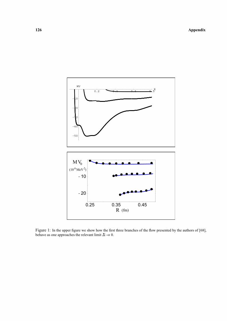
126 Appendix
0.2 0.3 0.4 0.5R
-50
-40
-30
-20
-10
MV
0.25 0.35 0.45
-20
-10
R (fm)
V0M26(10 MeV )
Figure 1: In the upper figure we show how the first three branches of the flow presented by the authors of [68],behave as one approaches the relevant limit � � 0.

Acknowledgments
A mi director de tesis, Joan Soto, por la oportunidad, la generosidad, la infinita paciencia. A mis
padres por el apoyo y la libertad, por seguir perdonandome, por matizar mis dıas negros. A mis
companeros de tercer ciclo, por la alegrıa y la complicidad.
Gracias.


Bibliography
[1] H. Georgi, Ann. Rev. Nucl. Sci. 43 (1995) 209; D. B. Kaplan, nucl-th/9506035; A. V. Manohar,
hep-ph/9606222; A. Pich, hep-ph/9806303; B.R. Holstein, nucl-th/0010015.
[2] N. Brambilla, hep-ph/0008279; V. Antonelli et al., Annals Phys. 286 (2001) 108; G. S. Bali, Phys.
Rept. 343 (2001) 1; A. Pineda, Nucl. Phys. Proc. Suppl. 93 (2001) 188.
[3] W. E. Caswell and G. P. Lepage, Phys. Lett. B 167 (1986) 437.
[4] B. Adeva et al., CERN-SPSLC-95-1; J. Schacher, hep-ph/9808407; A. Lanaro, � -N Newslett. 15
(1999) 270; M. Pentia et al., hep-ph/0001279.
[5] M. Knecht, B. Moussallam, J. Stern and N. H. Fuchs, Nucl. Phys. B 457 (1995) 513; Erratum-ibid.
B 471 (1996) 445; L. Girlanda, M. Knecht, B. Moussallam and J. Stern, Phys. Lett. B 409 (1997)
461.
[6] S. Weinberg, Physica A 96 (1979) 327; J. Gasser and H. Leutwyler, Ann. Phys. (N. Y.) 158 (1984),
142 and Nucl. Phys. B 250 (1985) 465.
[7] I. I. Kogan, A. Kovner and M. A. Shifman, Phys. Rev. D 59 (1999) 016001.
[8] D. Weingarten, Phys. Rev. Lett. 51 (1983) 1830.
[9] A. Dobado and J. R. Pelaez, Acta Phys. Hung. 8 (1998) 307.
[10] K. P. Arnold et al., Villigen Sin-Sin Newslett. 20 (1988) 38.
[11] L. L. Nemenov, Sov. J. Nucl. Phys. 41 (1985) 629.

130 Bibliography
[12] T. L. Trueman, Nucl. Phys. 26 (1961) 57; U. Moor, G. Rasche and W. S. Woolcock, Nucl. Phys.
A 587. (1995) 747; A. Gashi, G. C. Oades, G. Rasche and W. S. Woolcock, Nucl. Phys. A 628
(1998) 101 and Nucl. Phys. A 699 (2002) 732.
[13] H. Jallouli and H. Sazdjian, Phys. Rev. D 58 (1998) 014011; H. Sazdjian, hep-ph/9809425 and
Phys. Lett. B 490 (2000) 203.
[14] V. E. Lyubovitskij and A. G. Rusetsky, Phys. Lett. B 389 (1996) 181; V. E. Lyubovitskij, E. Z.
Lipartia and A. G. Rusetsky, JETP Lett. 66 (1997) 783; M. A. Ivanov, V. E. Lyubovitskij, E. Z.
Lipartia and A. G. Rusetsky, Phys. Rev. D 58 (1998) 094024.
[15] X. Kong and F. Ravndal, Phys. Rev. D 59 (1999) 014031 and Phys. Rev. D 61 (2000) 077506; B.
R. Holstein, Phys. Rev. D 60 (1999) 114030.
[16] A. Czarnecki, K. Melnikov and A. Yelkhovsky, Phys. Rev. A 59 (1999) 4316.
[17] J. Gasser, V. E. Lyubovitskij, A. Rusetsky and A. Gall, Phys. Rev. D 64 (2001) 016008.
[18] D. Eiras and J. Soto, Phys. Rev. D 61 (2000) 114027 and � N Newslett. 15 (1999) 181.
[19] S. Deser, M. L. Goldberger, K. Baumann and W. Thirring, Phys. Rev. 96 (1954) 774.
[20] A.V. Manohar, Phys. Rev. D 56 (1997) 230; A. Pineda and J. Soto, Phys. Rev. D 58 (1998) 114011.
[21] H. B. O’Connell, K. Maltman, A. W. Thomas and A. G. Williams, hep-ph/9707404.
[22] J. Bijnens, G. Colangelo, G. Ecker, J. Gasser and M. E. Sainio, Nucl. Phys. B 508 (1997) 263;
Erratum-ibid. B 517 (1998) 639; Phys. Lett. B 374 (1996) 210.
[23] M. Knecht and R. Urech, Nucl. Phys. B 519 (1998) 329.
[24] A. Pineda and J. Soto, Phys. Lett. B 420 (1998) 391 and Phys.Rev. D 59 (1999) 016005.
[25] M. B. Voloshin, Sov. J. Nucl. Phys. 36 (1982) 143; A. Pineda, Nucl. Phys. B 494 (1997) 213.
[26] H. Bateman, Higher Transcendental Functions Vol. I (1953) McGraw-Hill.
[27] P. Labelle and K. Buckley hep-ph/9804201.
Bibliography 131
[28] R. Baur and R. Urech, Nucl. Phys. B 499 (1997) 319.
[29] J. Bijnens and J. Prades, Nucl. Phys. B 490 (1997) 239; B. Moussallam, Nucl. Phys. B 504 (1997)
381.
[30] A. Gashi, G. Rasche, G. C. Oades and W. S. Woolcock, Nucl. Phys. A 628 (1998) 101.
[31] J. Gasser and H. Leutwyler, Phys. Lett. B 125 (1983) 325.
[32] J. Bijnens, G. Colangelo, G. Ecker, J. Gasser and M. E. Sainio, Phys. Lett. B 374 (1996) 210.
[33] G. Colangelo, J. Gasser and H. Leutwyler, Nucl. Phys. B 603 (2001) 125.
[34] M. M. Nagels et al., Nucl. Phys. B 147 (1979) 189.
[35] J. Bijnens et al., Phys. Lett. B 374 (1996) 210.
[36] A. Di Giacomo, Nucl. Phys. B 11 (1969) 411.
[37] A. Billoire, Phys. Lett. B 92 (1980) 343.
[38] M. B. Voloshin, Nucl. Phys. B 154 (1979) 365; H. Leutwyler, Phys. Lett. B 98 (1981) 447; A.
Pineda, Nucl. Phys. B 494 (1997) 213.
[39] A. H. Hoang, hep-ph/0008102.
[40] N. Brambilla, A. Pineda, J. Soto and A. Vairo, Phys. Rev. D 63 (2001) 014023.
[41] A. Pineda and A. Vairo, Phys. Rev. D 63 (2001) 054007; Erratum-ibid. D 64 (2001) 039902.
[42] N. Brambilla, Y. Sumino and A. Vairo, Phys. Lett. B 513 (2001) 381 and Phys. Rev. D 65 (2002)
034001.
[43] A. H. Hoang, A. V. Manohar, I. W. Stewart and T. Teubner, Phys. Rev. D 65 (2002) 014014.
[44] B. A. Kniehl, A. A. Penin, V. A. Smirnov and M. Steinhauser, hep-ph/0203166.
[45] N. Brambilla, A. Pineda, J. Soto, A. Vairo, Nucl. Phys. B 566 (2000) 275.
[46] S. Titard, F. J. Yndurain, Phys. Rev. D 49 (1994) 6007.
132 Bibliography
[47] G. E. Pustovalov, JETP 5 (1957) 1234.
[48] U. D. Jentschura, G. Soff, V.G. Ivanov, S. G. Karshenboim, Phys. Rev. A 56 (1997) 4483.
[49] S. G. Karshenboim, U. D. Jentschura, V.G. Ivanov, G. Soff, Eur. Phys. J. D 2 (1998) 209.
[50] R. D. Ball, Phys. Rept. 182 (1989) 1.
[51] K. Melnikov, A. Yelkhovsky, Phys. Rev. D 59 (1999) 114009.
[52] S. G. Karshenboim, Can. J. Phys. 76 (1998) 169.
[53] A. Pineda, F. J. Yndurain, Phys. Rev. D 58 (1998) 094022 and D 61 (2000) 077505.
[54] A. H. Hoang, A.V. Manohar, Phys. Lett. B 483 (2000) 94.
[55] A. H. Hoang et al., Eur. Phys. J. direct C 3 (2000) 1.
[56] M. Beneke et al., hep-ph/0003033.
[57] N. Gray, D. J. Broadhurst, W. Grafe and K. Schilcher, Z. Phys. C 48 (1990) 673.
[58] S. Weinberg, Phys. Lett. B 251 (1990) 288; Nucl. Phys. B 363 (1991) 3; Phys. Lett. B 295 (1992)
114.
[59] D. R. Phillips, S. R. Beane and T. D. Cohen, Annals Phys. 263 (1998) 255; D. R. Phillips, S. R.
Beane and M. C. Birse, J. Phys. A 32 (1999) 3397; J. V. Steele and R. J. Furnstahl, Nucl. Phys. A
637 (1998) 46.
[60] G. P. Lepage, CLNS-89-971, Jun. 1989 (TASI’89 Summer School Proc.) and nucl-th/9706029.
[61] U. van Kolck, Prog. Part. Nucl. Phys. 43 (1999) 337.
[62] N. Kaiser, S. Gerstendorfer, W. Weise, Nucl. Phys. A 637 (1998) 395.
[63] D. B. Kaplan, M. J. Savage and M. B. Wise, Nucl. Phys. B 478 (1996) 629.
[64] D. B. Kaplan, M. J. Savage and M. B. Wise, Phys. Lett. B 424, 390 (1998).
Bibliography 133
[65] S. Fleming, T. Mehen and I. W. Stewart, Nucl. Phys. A 677, 313 (2000); Phys. Rev. C 61 (2000)
044005.
[66] J. Gegelia, nucl-th/9806028; T. Mehen and I. W. Stewart, Phys. Lett. B 445 (1999) 378; D. B.
Kaplan and J. V. Steele, Phys. Rev. C 60 (1999) 064002.
[67] T. Frederico, V. S. Timoteo and L. Tomio, Nucl. Phys. A 653 (1999) 209.
[68] S. R. Beane, P. F. Bedaque, M. J. Savage and U. van Kolck, Nucl. Phys. A 700 (2002) 377.
[69] S. D. Glazek and K. G. Wilson, hep-th/0203088.
[70] H. E. Camblong et al., Phys. Rev. Lett. 85 (2000) 1590; Annals Phys. 287 (2001) 14 and 57.
[71] N. Brambilla, A. Pineda, J. Soto and A. Vairo, Phys. Lett. B 470 (1999) 215.
[72] N. Brambilla, A. Pineda, J. Soto and A. Vairo, Phys. Rev. D 60 (1999) 091502.
[73] S. R. Beane et al., Phys. Rev. A 64 (2001) 042103; D. W. L. Sprung et al., Phys. Rev. C 49 (1994)
2942.
[74] E. Epelbaum, W. Gl �
� ckle, Ulf-G. Meißner, Nucl. Phys. A 671 (2000) 295; Nucl.Phys. A 637
(1998) 107.
[75] A. Pineda and J. Soto, Nucl. Phys. B (Proc. Suppl.) 64 (1998) 428.
[76] G. T. Bodwin, E. Braaten and G. P. Lepage, Phys. Rev. D 46 (1992) R1914.
[77] G. T. Bodwin, E. Braaten and G. P. Lepage, Phys. Rev. D 51, (1995) 1125; E-ibid. D 55 (1997)
5853.
[78] R. Barbieri, R. Gatto and E. Remiddi, Phys. Lett. B 61 (1976) 465; R. Barbieri, M. Caffo and E.
Remiddi, Nucl. Phys. B 162 (1980) 220; R. Barbieri, M. Caffo, R. Gatto and E. Remiddi, Phys.
Lett. B 95 (1980) 93; Nucl. Phys. B 192 (1981) 61.
[79] N. Brambilla, D. Eiras, A. Pineda, J. Soto and A. Vairo, in preparation.
[80] A. Petrelli, M. Cacciari, M. Greco, F. Maltoni and M. L. Mangano, Nucl. Phys. B 514 (1998) 245;
F. Maltoni, PhD thesis (Univ. of Pisa, 1999) [http://web.hep.uiuc.edu/home/maltoni/thesis.ps].
134 Bibliography
[81] D. E. Groom et al., Eur. Phys. Jour. C 15 (2000) 1.
[82] M. Ambrogiani et al., Phys. Rev. D 62 (2000) 052002.
[83] R. Mussa, private communication; see also the talk at Charmonium spectroscopy: past and future,
Genoa, 7–8 June 2001 [http://www.ge.infn.it/charm2001/].
[84] G. T. Bodwin and Y. Chen, Phys. Rev. D 60 (1999) 054008 and Phys. Rev. D 64 (2001) 114008;
E. Braaten and Y. Chen, Phys. Rev. D 57 (1998) 4236.
[85] F. Maltoni, hep-ph/0007003.
[86] G. T. Bodwin, D. K. Sinclair and S. Kim, Int. J. Mod. Phys. A 12 (1997) 4019.
[87] G. T. Bodwin, D. K. Sinclair and S. Kim, Phys. Rev. D 65 (2002) 054504.
[88] M. Pentia, hep-ph/0001279.
[89] L. Rosselet et al., Phys. Rev. D 15 (1977) 574; M. M. Nagels et al., Nucl. Phys. B 147 (1979) 189.
[90] M. Luke and A. V. Manohar, Phys. Lett. B 286 (1992) 348.
[91] R. Sundrum, Phys. Rev. D 57 (1998) 331; M. Finkemeier, H. Georgi and M. McIrvin, Phys. Rev.
D 55 (1997) 6933; C. L. Lee, hep-ph/9709238.
[92] H. Georgi, Nucl. Phys. B 361 (1991) 339; M. Luke and A. V. Manohar, Phys. Lett. B 286 348; W.
Kilian and T. Ohl, Phys. Rev. D 50 (1994) 4649; C. Balzereit and T. Ohl, Phys. Lett. B 386 (1996)
335; C. Balzereit, hep-ph/ 9809226; ; S. Scherer and H. W. Fearing, Phys. Rev. D 52 (1995) 6445;
G. Ecker and M. Mojzis, Phys. Lett. B 410 (1997) 266 and Erratum-ibid. B 438 (1998) 446.