facoltàdi ingegneria, università degli studi di brescia
TRANSCRIPT

NOTES ON THE ENERGY BALANCE IN PHYSICAL LIMNOLOGY AND WATER QUALITY RELATED ISSUES
Prof. Marco Pilotti
Facoltà di Ingegneria, Università
degli Studi di Brescia

PHYSICAL LIMNOLOGY: Heat budget
M. Pilotti - NOTES ON ENGINEERING LIMNOLOGY
Some References
• B. Henderson-Sellers., Engineering limnology, Pitman Advanced Pub. Program,
1984, Boston
• S. Chapra, Surface Water Quality Modeling, Mc Graw Hill, 1997
On this topic and limnology in general master THESIS are available !

PHYSICAL LIMNOLOGY: Heat distribution and water properties
M. Pilotti - NOTES ON ENGINEERING LIMNOLOGY
Let us introduce in a pot the same amount of heat from two opposite direction
Will the final T distribution be different ?
If the water is originally quiet,
the hydrostatic equation holds
According to which, surface
where p=C1 are also
characterized by ρ= C2 and
T = C3. The difference is tied
to the stability of the equilibrium.
The final flow field and the heat
distribution are totally different.
The reason is in the equation of state
∫ ⋅S
dSnqrr
0=∇+∇− pzgρ

PHYSICAL LIMNOLOGY: Heat budget
M. Pilotti - NOTES ON ENGINEERING LIMNOLOGY
Water density ρ(p,T,S,s)
P: pressure; T:temperature [°C]; S:dissolved salts; s:suspendend particles
an easy and rough approximation is
That shows that it is primarily a function of T . Accordingly, it is important to introduce the
Thermal Expansivity [K-1]
A first order approximation is
SPSP TT
V
V ,, )1
()1
(∂∂−=
∂∂= ρ
ρα
20 )4(007.01000 CT °−−=ρ
)4(014.01000
1CT °−≅α

PHYSICAL LIMNOLOGY: Heat budget
M. Pilotti - NOTES ON ENGINEERING LIMNOLOGY
For fresh water, Chen_and_Millero (1977) provided an experimental equations with a precision
better than 0.002 Kg/mc in the field of interest of limnology
(0-30 °C, 0-600 ppm, g/kg Total dissolved Solids, 0-180 bars)
ρ0 is the density at the surface
to optain the density at pressure p one applies the correction
to take into account the increase of density when suspended solids are present (C is the
solid concentration in kg/m3)
when sediments are quartz made
( )2654320 lTiThSgTfTeTdTcTbTa +−+−+−+−+=ρ
[ ] ( ) ( )MpLTISHTGTFpETDTCTBTAbar
pp
+−++−+−+−+=
−=
2432
0 1
1)(
εε
ρρ
[ ] CVV
VC
ssss
ss
−=−+−=∆
=
ρρρρρρ
ρ
1)1(
/
C63.0=∆ρ
PHYSICAL LIMNOLOGY: Heat budget
M. Pilotti - NOTES ON ENGINEERING LIMNOLOGY
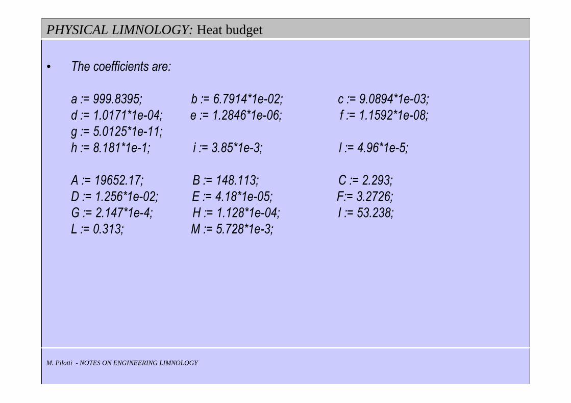
• The coefficients are:
a := 999.8395; b := 6.7914*1e-02; c := 9.0894*1e-03;
d := 1.0171*1e-04; e := 1.2846*1e-06; f := 1.1592*1e-08;
g := 5.0125*1e-11;
h := 8.181*1e-1; i := 3.85*1e-3; l := 4.96*1e-5;
A := 19652.17; B := 148.113; C := 2.293;
D := 1.256*1e-02; E := 4.18*1e-05; F:= 3.2726;
G := 2.147*1e-4; H := 1.128*1e-04; I := 53.238;
L := 0.313; M := 5.728*1e-3;

PHYSICAL LIMNOLOGY: Heat budget
M. Pilotti - NOTES ON ENGINEERING LIMNOLOGY

PHYSICAL LIMNOLOGY: Heat budget
M. Pilotti - NOTES ON ENGINEERING LIMNOLOGY
• T(z) is possibly the most important physical aspects for lake modelling
• This is a consequence of the EOS of water
• It determines vertical stability, so conditioning vertical dynamics and vertical exchange
of chemical quantities (O2, P,…) and biological activity, which is also conditioned by
light availability
• The evolution into Epilimnion, Metalimnion and Hypolimnion is a consequence of energy
fluxes and thermocline deepening by turbulent mixing and direct absorption of solar
radiation
• Positive energy balance in summer and negative in late summer when convective
cooling start
• Dimictic (2 overturns) and monomictic (1 overturn) lakes
• Polymictic (several times in a year), Oligomictic (rarely), Meromictic (never)

PHYSICAL LIMNOLOGY: Heat budget
M. Pilotti - NOTES ON ENGINEERING LIMNOLOGY
• The other fundamental driver of the lake is wind, that interacts with the T structure
to determine the flow field
Summ
er Winter
Summ
er Winter
Summ
er Winter
Summ
er Winter
Summ
er Winter
Summ
er Winter
Summ
er Winter
Summ
er Winter

PHYSICAL LIMNOLOGY: Heat budget
M. Pilotti - NOTES ON ENGINEERING LIMNOLOGY
• Is Iseo lake getting meromictic ?

PHYSICAL LIMNOLOGY: Heat budget and T(z)
M. Pilotti - NOTES ON ENGINEERING LIMNOLOGY
][JTmCQU p∆=∆=∆ Q is the variation of heat content of a mass m and is an
extensive property. Its value depends on the specific heat
Cp [J/(kgK)]. Note the value of Cp below. (1) is the amount
of heat needed to cause a 1 °C rise of 1 m3 of substance
∫∫∫∫∫∫ +⋅+⋅+⋅=+WSS
n
WWW
hdWdSnqdSvdWvgdWvDt
DudW
Dt
D rrrrrr σρρρ 2
2
1
To understand better and to generalize we must start from the I law of thermodynamics for
a control system contained within a volume W limited by a surface S (e.g., a pool of water)
(symbols as in Hydraulics Class: u internal energy for unit mass, v local velocity,
σn local stress associated to direction n, q vector of energy flux along the boundary and h
internal source of thermal energy
U = internal energy ρ ρ ρ ρ Cp λ λ λ λ (1)
kg/m3 J/(kg K)))) W/(m K)))) Jair 1.164 1012 0.0255 1177.968water 998.2 4182 0.604 4174472brick 1800 840 0.6-1.4 1512000cast iron 7272 420 62 3054240
Thermal conductivity

PHYSICAL LIMNOLOGY: Heat budget
M. Pilotti - NOTES ON ENGINEERING LIMNOLOGY
Considering that u when p
is constant is tied through
the specific heat, one can write
that is a simple thermal balance
or the control system in W
∫∫∫∫ +⋅+⋅=∂∂
WSSW
hdWdSnqdSnvuudWt
rrrrρρ
∫ ⋅S
dSnqrr
When the velocity and the power of shear stress are negligible this equation can be simplified
and rewritten (Reynolds’ Theorem) as
∫∫∫∫ +⋅+⋅=∂∂
WSS
p
W
p hdWdSnqdSnvTCTdWCt
rrrrρρ
Rate of change of thermal energy
within the control volume
Flux of thermal energy through the boundary connected to a flux of mass
Flux of heat through the boundary not connected to mass flux; [q]=W/m2
(e.g., through convective transfer, evaporation, solar radiation)
Internal heat source (absorption of shortwave radiation)
∫∂∂
W
pTdWCt
ρ
∫ ⋅S
p dSnvTCrrρ
∫W
hdW
(1)
(2)
(3)
(4)
(5)
(6)

PHYSICAL LIMNOLOGY: Heat budget
M. Pilotti - NOTES ON ENGINEERING LIMNOLOGY
∫ ⋅=S
N dSnqrrφ
• In reality term (5) is made up of different contributions that must be considered
separately. We shall neglect exchange at the bottom and we shall integrate these
contributions on a daily basis.
• This terms can be grouped as Radiation terms and Nonradiation terms
• Radiation terms: Solar Shortwave, Atmospheric Longwave, Lake Longwave
• Nonradiation terms: Conduction and convection, Evaporation and Condensation
• Conduction and convection: Sensible heat
• Evaporation and Condensation: Latent heat
• They can be grouped also depending on their dependence on water T

PHYSICAL LIMNOLOGY: Heat budget
M. Pilotti - NOTES ON ENGINEERING LIMNOLOGY
∫ ⋅=S
N dSnqrrφ
pcerrN φφφφφφφ +−−−+= 120
2rφ1rφeφ
cφ
pφ
: net Short Wave radiation, incident - reflected
: net incoming Long Wave radiation from atmosphere molecules and clouds
: Long Wave radiation loss from the lake
: evaporation (latent heat)
: conduction and convection (sensible heat)
: precipitation
The net flux is made up of
)1(0 SS A−= φφ

PHYSICAL LIMNOLOGY: Heat budget - radiation
M. Pilotti - NOTES ON ENGINEERING LIMNOLOGY
]/[),0,(
18
),,(
24
1
521
2
1
mWTTE
dehc
TE kT
hc
εσ
λλπλλ λ
λ
λ
=∞
−=
−
∫
h : Planck’s constant
c : light speed
σ : Stefan Boltzmann constant
(5.67x10⁻⁸ W/(m2K4))
ε : body emissivity

PHYSICAL LIMNOLOGY: Heat budget -net Short Wave radiation
M. Pilotti - NOTES ON ENGINEERING LIMNOLOGY
The lake is driven by incoming shortwave radiation and by wind
The average daily SW at the top of atmosphere can be
computed in a very precise way as a function of the latitude
and of the period of the year
The average daily SW at the ground depends
on transmission through the atmosphere, and depends
on the ditribution of aerosol and cloud type and cover.
Accordingly, it is very difficult to compute it without
accurate information on the atmosphere
The net SW entering the lake depends on reflectivity As.
Alternatively and relaibly, SW can
be measured with a net radiometer
As a first guess, use As=0.06. However it varies significantly
depending on the height of the sun on the horizon
Sφ
)1(0 SS A−= φφ

PHYSICAL LIMNOLOGY: Heat budget -net Short Wave radiation
M. Pilotti - NOTES ON ENGINEERING LIMNOLOGY
The fraction β of SW radiation captured in the first layer
is about 0.4 - 0.5. More realistically, it depends on
water turbidity (sediments, fito- zoo plankton)
Where η is the extinction coefficient, that is a measure
of the rate of absorption of light under the surface
(Beer’s law)
η is seldom measured. Usually it is estimated on the
basis of Sechi disk depth d, on the basis of some
empirical correlations
614.0)ln(265.0 += ηβ
( ) zez ηφβφ −−= 01)(
73.0/1.1
/7.1
d
d
=
=
ηη

PHYSICAL LIMNOLOGY: Heat budget -net Short Wave radiation
M. Pilotti - NOTES ON ENGINEERING LIMNOLOGY

PHYSICAL LIMNOLOGY: Heat budget -Long Wave radiation
M. Pilotti - NOTES ON ENGINEERING LIMNOLOGY
Due to its temperature, almost all the electromagnetic energy emitted by the lake has a
wave length λ > 4µm (Longwave)
The overall radiative loss of the lake is
σ : Stefan Boltzmann constant (5.67x10⁻⁸W/(m2K4))
εw: water emissivity (0.97)
In a similar way, the incoming longwave radiation is the reradiated energy emitted by
clouds and atmosphere
εa: air emissivity
Ta: effective air T
Provided that clouds and aerosols at different height (and so at different T) contribute, the
T of the air is an effective one.
Several empirical relationship have been proposed as a function of relative humidity for
cloudless skies or of Cloud Cover.
41 wwr Tσεφ =
4aar Tσεφ =

PHYSICAL LIMNOLOGY: Heat budget -Evaporative flux
M. Pilotti - NOTES ON ENGINEERING LIMNOLOGY
( )[ ] ]/[1000273365.29.2500 kgJTL
EL
wV
Ve
⋅−−== ρφ
Evaporation E [m/s] causes a significative energy loss, as recognised by Dalton (1802), who
observed that it is a function of wind speed and that more water can be evaporated if the
air mass is relatively dry. When the air gets in contact with water, its umidity grows and
its efficiency in absorbing vapor decreases
LV is the Latent Heat of Vaporizati
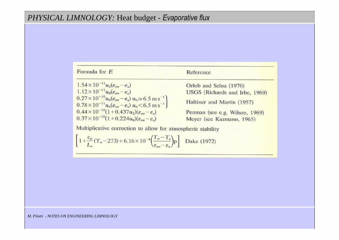
Several formulas are available for evaluating E, most with structure
esw = saturated vapour pressure at T of water
ea actual vapour pressure at T of air
W = wind speed
]/[))(( smeewfCE asw −⋅=
PHYSICAL LIMNOLOGY: Heat budget -Evaporative flux
M. Pilotti - NOTES ON ENGINEERING LIMNOLOGY
PHYSICAL LIMNOLOGY: Heat budget -Evaporative flux
M. Pilotti - NOTES ON ENGINEERING LIMNOLOGY
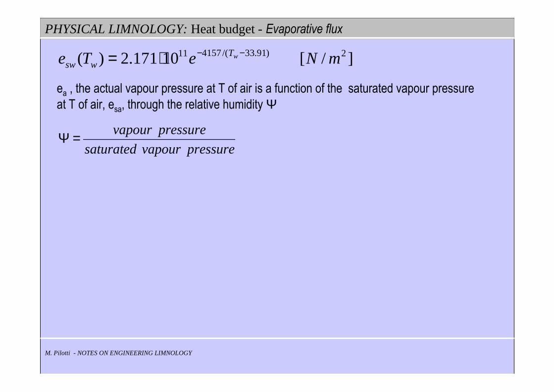
ea , the actual vapour pressure at T of air is a function of the saturated vapour pressure
at T of air, esa, through the relative humidity Ψ
]/[10171.2)( 2)91.33/(415711 mNeTe wTwsw
−−⋅=
pressurevapoursaturated
pressurevapour=Ψ
PHYSICAL LIMNOLOGY: Heat budget -Sensible heat
M. Pilotti - NOTES ON ENGINEERING LIMNOLOGY
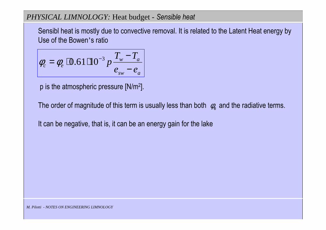
Sensibl heat is mostly due to convective removal. It is related to the Latent Heat energy by
Use of the Bowen’s ratio
p is the atmospheric pressure [N/m2].
The order of magnitude of this term is usually less than both φe and the radiative terms.
It can be negative, that is, it can be an energy gain for the lake
asw
awec ee
TTp
−−⋅⋅= −31061.0φφ

PHYSICAL LIMNOLOGY: Heat budget -measure of radiation
M. Pilotti - NOTES ON ENGINEERING LIMNOLOGY

PHYSICAL LIMNOLOGY: Heat budget -variability of the contributions during the year
M. Pilotti - NOTES ON ENGINEERING LIMNOLOGY
pcerrN φφφφφφφ +−−−+= 120

PHYSICAL LIMNOLOGY: Heat budget
M. Pilotti - NOTES ON ENGINEERING LIMNOLOGY
Let us now suppose that our control system is a completely stirred tank (CST), so that
variables vary only in time. If Cp and ρ are kept constant, Equation (2) can be written as
( ) ( ) ( ) hWqSQTCTQCWTdt
dC outpinpp ++−= ρρρ
( )inp TQCρ
That must be solved along with the mass balance equation, where Q is the volumetric flow
discharge entering or flowing out of the lake ( [Q]=m3/s )
outpTQCρ Outflow of thermal energy connected to the volumetric flow
discharge flowing out of the lake with the temperature of the lake
ERQQdt
dWoutin −+−=
Sources of thermal energy connected to the volumetric flow
discharge entering the lake; [Q]=m3/s
And where R is the rainfall and E the evaporation from the surface. In the following these two
terms will be supposed equal, for simplicity’s sake, and so can be dropped.
qS Energy exchange across the lake’s boundary (surface, sediments)
(7)
(8)
(9)
(10)
(11)

PHYSICAL LIMNOLOGY: Heat budget
M. Pilotti - NOTES ON ENGINEERING LIMNOLOGY

PHYSICAL LIMNOLOGY: Heat budget - example - Lake Iseo
M. Pilotti - NOTES ON ENGINEERING LIMNOLOGY
Let us now suppose Iseo lake is at steady state. It is straightforward to obtain from (7) the
equilibrium temperature of the lake
( )( )
( )( ) ( ) ][KT
QC
hWqS
Q
TQ
QC
hWqSTQC
outpout
in
outp
inp =++=++
ρρρ
( ) ( ) ( )( )
( )( )
CQ
TQ
sCmTQ
dtTQTQTQ
out
in
in
CanaleOglio
in
°==
°=
++= ∫
87.95.60
95.596
95.596
3653
365
1
smQ
sm
dtQQ
sm
dtQQ
Out
Canale
Canale
Oglio
Oglio
3
3
365
1
3
365
1
5.60
9.30365
6.29365
=
==
==
∫
∫
Note that here it is unrelevant whether °C or K
are used on both sides. We shall suppose h =0;
S = 61*106 m2

PHYSICAL LIMNOLOGY: Heat budget - example - Lake Iseo
M. Pilotti - NOTES ON ENGINEERING LIMNOLOGY
2
365
1 12.130365 m
WdtSWSW == ∫
2
365
1 5.44365 m
WdtLWLW −== ∫
2
365
1
2
365
1
05.46365
54.3365
mWdtLH
LatentHeat
mWdtSH
atSensibleHe
−==
−==
∫
∫
Note that net LW is properly given by
If one uses ε= 0.97 and the time series of water T at the
surface, one can compute the effective Ta of atmosphere;
Ta=278.24 K=5.08 °C
( )365
365
1
44 dtTTLW
aw∫ −−=
εσ

PHYSICAL LIMNOLOGY: Heat budget - example - Lake Iseo
M. Pilotti - NOTES ON ENGINEERING LIMNOLOGY
Regarding heat geothermal flux, Livingstone, (1997) computed for Lake Geneve and Zurich
0.07 - 0.13 W/m2. So this contribution can be disregarded.
At steady state the Lake Iseo temperature would be
( )( )
( )[ ]( ) ( )448-448-
644
24.278101.3284-44.4024.278101.3284-45.9187.95.6041822.998
106124.27853.80
87.9 −⋅=−⋅+=⋅⋅⋅−−
+=+
= eqeq
eq
out
pin
eq TT
T
Q
CqS
TQ
T
εσρ
That has solution T = 16.03 °C. Under this condition the whole energy entering from the
lake surface would be taken away by the outflow and lost as LW radiation and Latent Heat.
This result is in contradiction with the volume weighed yearly average Iseo lake that is
T is about 7.4 °C.
Note that equation (7) at equilibrium is not a function of W (if h= 0). Being perfectly stirred,
all the lake is supposed to be at the same T
Iseo lake is not a CSTR (completely stirred tank reactor) and is never at equilibrium

PHYSICAL LIMNOLOGY: Heat budget and T vertical profile
M. Pilotti - NOTES ON ENGINEERING LIMNOLOGY
Let us consider a cilindrical lake with area A and adiabatic boundary. The upper
surface is limited by the atmosphere. No other thermal input is present.
Is it possible to determine the evolution in time of the thermal profile T(z) ?
Let us start from equation (2), that we simplify with the same ipothesis that led to
eq. (1)
Now we apply a consequence of mass conservation and of Reynolds Theorem (see
hydraulics class)
But these terms can be rewritten as
∫∫∫ +⋅=WSW
p hdWdSnqTdWCDt
D rrρ
∫∫∫ +⋅=WSW
p hdWdSnqdWDt
DTC
rrρ
∫∫∫ +⋅∇−=
∇+∂∂
WSW
p hdWdSnTdWTvt
TC
rλρ(I1)

PHYSICAL LIMNOLOGY: Heat budget and T vertical profile
M. Pilotti - NOTES ON ENGINEERING LIMNOLOGY
Where we have considered the definition of material derivative
and the Fick’s law for molecular diffusion (see tipical values before)
Now let us apply gradient’s theorem (again, see hydraulics class)
And accordingly
Tvt
T
Dt
DT ∇+∂∂=
Tq ∇−= λr
∫∫ ∇=⋅∇−WS
dWTdivdSnT )(λλ r
∫ =
−∇−
∇+∂∂
W
p dWhTdivTvt
TC 0)(λρ
∫∫∫ +∇=
∇+∂∂
WWW
p hdWdWTdivdWTvt
TC )(λρ

PHYSICAL LIMNOLOGY: Heat budget and T vertical profile
M. Pilotti - NOTES ON ENGINEERING LIMNOLOGY
Which is clearly equivalent to the PDE
Let us now suppose that λ is constant and let us remember that our system is 1D with
variation only as a function of z. Accordingly v has only the vertical component w (should be 0)
This is a parabolic convection-diffusion PDE that, to be solved, requires the flow field (w)
and appropriate initial condition T0(z) and boundary conditions. The natural boundary
conditions are related to the heat flux for z= 0 and z=Zmax; alternatively, the latter can be
substituted by T(t, Zmax) (T at the bottom) that usually can be regarded as constant.
( )hTdivC
Tvt
T
hTdivTvt
TC
p
p
+∇=∇+∂∂
=−∇−
∇+∂∂
)(1
0)(
λρ
λρ
pp C
h
z
T
Cz
Tw
t
T
ρρλ +
∂∂=
∂∂+
∂∂
2
2
(I2)

PHYSICAL LIMNOLOGY: Heat budget and T vertical profile
M. Pilotti - NOTES ON ENGINEERING LIMNOLOGY
Equation (I2) can be integrated numerically to produce T(z) as required.
In order to do it, we must approximate numerically (I2): although in this case this is not a
difficult task we shall pursue a different, more productive road
Equations (I1) and (I2) seems physically equivalent. However, (I1) is a property of a finite
volume and (I2) is a punctual properties (!). From the mathematical point of view they are
not equivalent. E.g., (I2) requires that T(z) belongs to C2 in z and (I1) doesn’ t.
Is it possibly better to solve eq. (I1) ? To decouple the problem from the flow field, let us
suppose that w= 0, as it should be strictly from continuity.
where is the thermal diffusivity [m2/s].
∫∫∫ +⋅∇−=∂∂
W pS pW
dWC
hdSnT
CTdW
t ρρλ r
pCρλ
(I3)

PHYSICAL LIMNOLOGY: Heat budget and T vertical profile
M. Pilotti - NOTES ON ENGINEERING LIMNOLOGY
To start with, (I3) can be applied to any of the arbitrary control volumes
into which our original water column is decomposed
The water column is decomposed into arbitrary i control volumes (CV),
which have the upper and lower surface in common with the preceeding
and following CV.
Where we consider the following rule for n
Now the problem is that of computing terms (A), (B) and (C). This will be
done in the next Classwork where equation (I3) will be solved, in order to
determine the T(z,t) profile .pCρ
λ
∫∫∫∫ +
∇−∇−=
∂∂
Wi pSi pSi pWi
dWC
hTdS
CTdS
CTdW
t ρρλ
ρλ
21
(A) (B) (C)

STREETER-PHELPS: Organic production-decomposition
M. Pilotti - NOTES ON WATER QUALITY MODELING
Molecular weightsH 1C 12N 14O 16P 31S 32
Ca 40
Carbon dioxide +
(1)
(2)
STREETER-PHELPS: Organic production-decomposition
M. Pilotti - NOTES ON WATER QUALITY MODELING
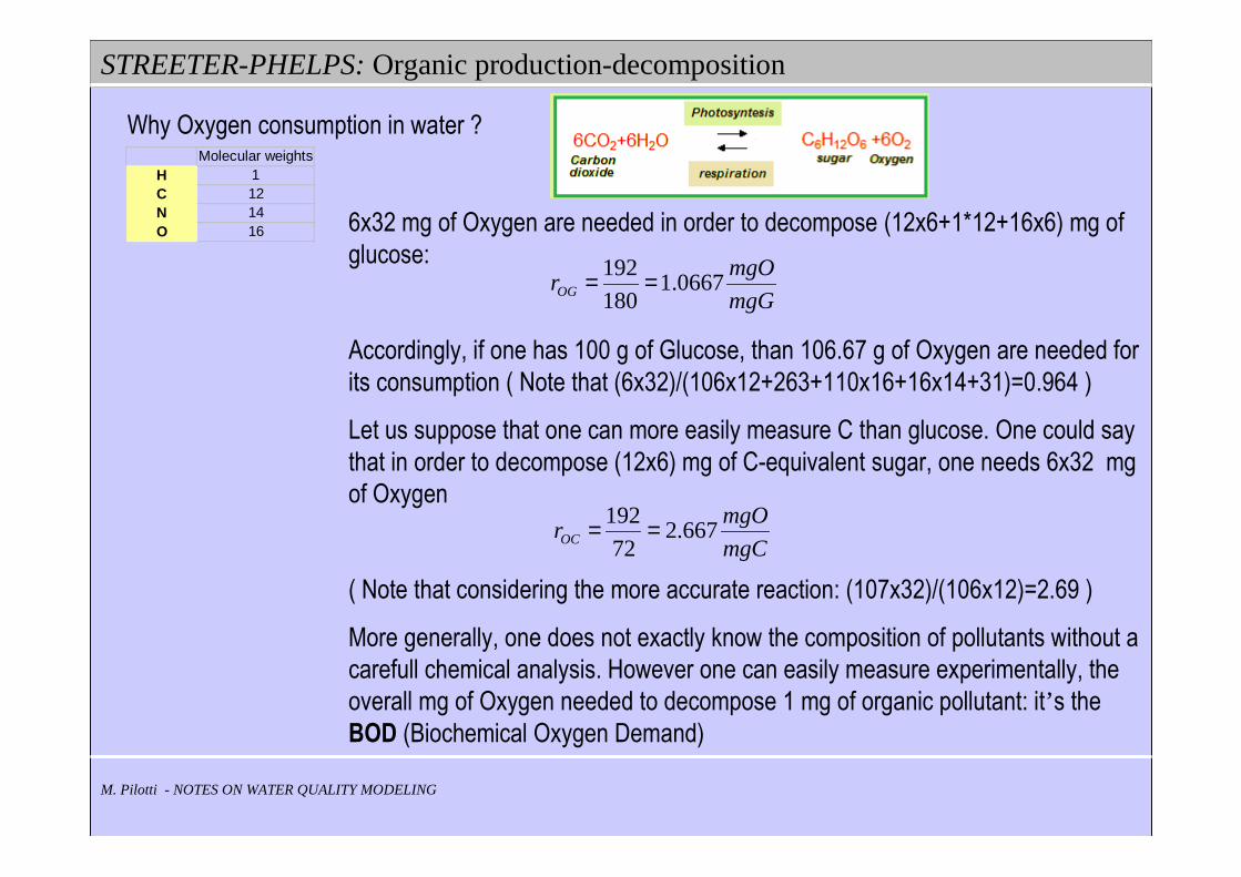
6x32 mg of Oxygen are needed in order to decompose (12x6+1*12+16x6) mg of
glucose:
Accordingly, if one has 100 g of Glucose, than 106.67 g of Oxygen are needed for
its consumption ( Note that (6x32)/(106x12+263+110x16+16x14+31)=0.964 )
Let us suppose that one can more easily measure C than glucose. One could say
that in order to decompose (12x6) mg of C-equivalent sugar, one needs 6x32 mg
of Oxygen
( Note that considering the more accurate reaction: (107x32)/(106x12)=2.69 )
More generally, one does not exactly know the composition of pollutants without a
carefull chemical analysis. However one can easily measure experimentally, the
overall mg of Oxygen needed to decompose 1 mg of organic pollutant: it’s the
BOD (Biochemical Oxygen Demand)
Why Oxygen consumption in water ?
mgG
mgOrOG 0667.1
180
192==
mgC
mgOrOC 667.2
72
192==
Molecular weightsH 1C 12N 14O 16
STREETER-PHELPS: Organic production-decomposition: Glucose in a CSTR
M. Pilotti - NOTES ON WATER QUALITY MODELING
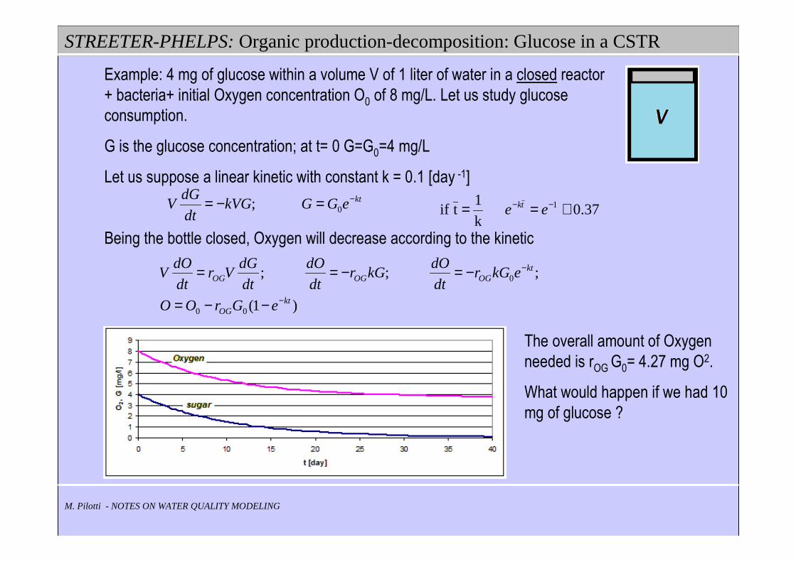
Example: 4 mg of glucose within a volume V of 1 liter of water in a closed reactor
+ bacteria+ initial Oxygen concentration O0 of 8 mg/L. Let us study glucose
consumption.
G is the glucose concentration; at t= 0 G=G0=4 mg/L
Let us suppose a linear kinetic with constant k = 0.1 [day -1]
Being the bottle closed, Oxygen will decrease according to the kinetic
kteGGkVGdt
dGV −=−= 0;
)1(
;;;
00
0
ktOG
ktOGOGOG
eGrOO
ekGrdt
dOkGr
dt
dO
dt
dGVr
dt
dOV
−
−
−−=
−=−==
The overall amount of Oxygen
needed is rOG G0= 4.27 mg O2.
What would happen if we had 10
mg of glucose ?
37.0k
1tif 1 ≅== −− ee tk

STREETER-PHELPS: Organic production-decomposition: CBOD in a closed CSTR
M. Pilotti - NOTES ON WATER QUALITY MODELING
However, sewage is not made up simply of sugar. It is not practical to think at a detailed analysys
of its component and a detailed determination of the decompostion rate. Traditionally, a lumped
approach was favoured.
L = amount of Oxidizable matter expressed in terms of Oxygen equivalent [mgO/L], to be
determined experimentally. Given that it might be easy to measure Corg, the organic carbon
concentration, sometimes
BOD(t) = y(t) = L0 -L(t) is the Oxygen consumed.
Accordingly, L0 can be seen either as the initial amount of oxidizable matter or as the final BOD,
BOD∞, when all the organic matter has been consumed.
Note that 0.05 <= k1 <= 0.5 [d-1], but faster for rivers. Accordingly, measuring L0 or BOD∞ would
take too long, so that usually BOD5 is measured and BOD∞ computed as
−=−=
=
=
−=−
−
tk
tk
eLkLkdt
dOeLL
dt
dL
dt
dO
VLkdt
dLV
1
1
011
01 ( )
−−=−==
−
−∞
−
)1(
1;1
11
00
0tk
tktk
eLOO
eBODBODeLL
orgorgOC CCrL 667.2==
( )155 1/ keBODBOD −
∞ −=
STREETER-PHELPS: BOD and flowing water
M. Pilotti - NOTES ON WATER QUALITY MODELING
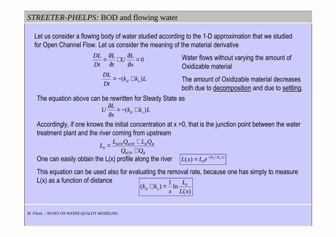
Let us consider a flowing body of water studied according to the 1-D approximation that we studied
for Open Channel Flow. Let us consider the meaning of the material derivative
0=∂∂+
∂∂=
x
LU
t
L
Dt
DL Water flows without varying the amount of
Oxidizable material
The amount of Oxidizable material decreases
both due to decomposition and due to settling.
LkkDt
DLsd )( +−=
The equation above can be rewritten for Steady State as
Accordingly, if one knows the initial concentration at x =0, that is the junction point between the water
treatment plant and the river coming from upstream
One can easily obtain the L(x) profile along the river
This equation can be used also for evaluating the removal rate, because one has simply to measure
L(x) as a function of distance
Lkkx
LU sd )( +−=
∂∂
RWTP
RRWTPWTP
QLQLL
++=0
xkk sdeLxL )(0)( +−=
)(ln
1)( 0
xL
L
xkk sd =+

STREETER-PHELPS: BOD and flowing water with reareation
M. Pilotti - NOTES ON WATER QUALITY MODELING
Let us consider a flowing body of water studied according to the 1-D approximation that we studied
for Open Channel Flow. Let us now consider Oxygen reareation. Here we shall make use of the
symbol d/dt but we make reference to the lagrangian meaning D/Dt
LkLkkdt
dLrsd −=+−= )(
The amount of Oxidizable material decreases due to decomposition and
settling
Let us consider Oxygen dynamics: note that O decreases only due to
decomposition (kd in place of kr !); On the other hand we have a
reareation as (e.g. O‘Connor-Dobbins formula, with U [m/s], Y [m])
the problem analitically simplifies if we introduce the Oxygen deficit D; let
us suppose that at station 0, L=L0 and D =D0
)( OOkLkdt
dOSad −+−=
dOdDOOD S −=−= );(
+=+
=
−+=
−=−
−
tkda
tk
ad
r
r
r
eLkDkdt
dDeLL
DkLkdt
dD
Lkdt
dL
0
0
+−−
=
=−−−
−
tktktk
ra
d
tk
aar
r
eDeekk
LktD
eLtL
00
0
)()(
)(
][93.3 15.1
5.0−= d
Y
Uka
Oxygen sag curve

M. Pilotti - NOTES ON WATER QUALITY MODELING
If we keep in mind that the time derivative from which we started are substantial derivative, we can
immediately pass from time to space
If U, the water velocity, is constant, then t=x/U, so that the space distribution of L and D is
Finally, if u=u(x) and U is the space average velocity then x =tU and
But if u=u(x) possibly also the coefficients vary in space so that a numerical solution is advisable
∫=L
udxL
U0
1
+−−
=
=−−−
−
tktktk
ra
d
tk
aar
r
eDeekk
LktD
eLtL
00
0
)()(
)(
+−−
=
=−−−
−
U
xk
U
xk
U
xk
ra
d
U
xk
aar
r
eDeekk
LkxD
eLxL
00
0
)()(
)(
∫= L
udx
xLt
0
+−−
=
=
∫
−∫
−∫
−
∫
−
LaLaLr
Lr
udx
xLk
udx
xLk
udx
xLk
ra
d
udx
xLk
eDeekk
LktD
eLtL
000
0
00
0
)()(
)(
STREETER-PHELPS: BOD and flowing water with reareation

M. Pilotti - NOTES ON WATER QUALITY MODELING
STREETER-PHELPS: effects on the environment of sewage treatment plant effluent

M. Pilotti - NOTES ON WATER QUALITY MODELING
Accordingly, there is a critical station where D is maximum and Oxigen content minimum. This
happens in correspondence of a critical travel time, tc
that can be easily obtained by setting so obtaining
By substituting within D(t) one gets the critical deficit as
The analysis is simplified if D0=0
tktktk
ra
d aar eDeekk
LktD −−− +−
−= 0
0 )()(
( )
−−−
=0
01ln1
Lk
kkD
k
k
kkt
d
ra
r
a
rac
0)( =
dt
tdD
( ) ra
r
kk
k
d
ra
r
a
a
dc Lk
kkD
k
k
k
LkD
−−
−−=0
00 1
ra
r
kk
k
r
a
a
dc
r
a
rac k
k
k
LkD
k
k
kkt
−−
=
−= 0;ln
1
STREETER-PHELPS: BOD and flowing water with reareation

STREETER-PHELPS: BOD and flowing water
M. Pilotti - NOTES ON WATER QUALITY MODELING
D has been introduced to simplify the equation: D= Os-O. However, Os is a function of several
variables, most noticeably of T. In fresh water at 1 ATM, the relationship holds (APHA, 1992)
Where T is in Kelvin.
4
11
3
10
2
75
s
10*8.621949-
10*1.2438+
10*6.642308-
10*1.575701+-139.34411)ln(O
aaaa TTTT=
Accordingly, when using Streeter Phelps
model, one has to pay attention at junctions,
where an Oxygen balance must be
accomplishedSource river
Q (m3/s) 0.463 5.787T [°C] 28 20DO [mg/L] 2 7.5DO sat. [mg/L] 7.827 9.092DO deficit [mg/L] 5.827 1.592
LmgDOLmgO
LmgO
CT
deficitS /093.7987.8;/987.8)59.20(
/093.7787.5463.0
5.7787.52463.0
59.20787.5463.0
20787.528463.0
22
2
2
−==
=+
⋅+⋅=
°=+
⋅+⋅=

STREETER-PHELPS: BOD and flowing water
M. Pilotti - NOTES ON WATER QUALITY MODELING
Let us consider a river where geometrical features change with distance from the source and where
a concentrated effluent enters at the upstream end point. What will be the O(x) pattern along the
river ? See Classwork 10
0
200
400
600
800
1000
1200
1400
1600
0 10000 20000 30000 40000 50000 60000 70000 80000
x [m]
A [
km2 ]

NITROGEN: effects on Water Quality
M. Pilotti - NOTES ON WATER QUALITY MODELING
•Effects on Oxygen content: nitrification decreases available Oxygen
•Effects on Eutrophication: availability of primary components
•Nitrate pollution: NO3-in drinking water
•Ammonia toxicity: ammonia gas (NH3) toxicity for fish

NITROGEN: effects on Oxygen Content
M. Pilotti - NOTES ON WATER QUALITY MODELING
• Autotrophic bacteria assimilate the ammonia through nitrification
mgN
mgOr
mgN
mgOr
Oi
Oa
14.114
325.0
43.314
325.1
=⋅=
=⋅=
• accordingly, a more complete assesment of Oxygen consumption must take into account also
Nitrogen nitrification. If we consider only the nitrogen arising from organic matter decay
•The primary consumption is given by 107x32/(106x12) but in addition 16 atoms of N are produced
every 106 of C. Accordingly a more complete figure is
mgC
mgO5.38.069.257.4
12106
1416
12106
32107 =+=⋅⋅⋅+
⋅⋅ So Oxygen consumption due to nitrification accounts
for 0.8/2.69=0.297 of the overall Oxygen
consumption.
mgN
mgOrrr OiOaOn 57.4=+=

NITROGEN: CBOD and NBOD
M. Pilotti - NOTES ON WATER QUALITY MODELING
• Bod can be due both directly to organic matter decomposition (CBOD) and to the following
nitrification (NBOD). However, often N in nitrogen comes from non organic sources. Accordingly,
CBOD and NBOD could have similar values (e.g., 220 mg/L for untreated sewage in develop
countries)
•However, a Streeter Phelps model for NBOD would be unsatisfactory because it is too far from the
actual process that leads to Oxygen consumption due to Nitrogen. The process has a dynamics in
time
•For instance, in a sewage we may have only Organic matter and in such a case nitrification take
longer because first we have to produce Ammonium first.
In another sewage we may have the same amount of nitrogen but directly as Ammonium. In that
case the process is faster.
•Finally, nitrification is strongly conditioned by other cofactors, such as Oxygen concentration or
pH, that can slow down or hinder the process.
•Accordingly, a more detailed representation than a Streeter Phles model is preferred for
nitrification

NITROGEN: CBOD and NBOD
M. Pilotti - NOTES ON WATER QUALITY MODELING

NITROGEN: Modeling Nitrification
M. Pilotti - NOTES ON WATER QUALITY MODELING
•Assuming first order kinetics, the nitrification process can be represented as
And the Oxygen deficit connected to Nitrogen can be represented as
=
−=
−=
−=
iinn
iinaaii
aaiooaa
ooao
Nkdt
dN
NkNkdt
dN
NkNkdt
dN
Nkdt
dN Organic matter (No) decay
Ammonium (Na) production and decay as nitrite
Nitrite (Ni) production and decay as nitrate
Nitrate (Nn) growth
DkNkrNkrdt
dDaiinoiaaioa −+=
Typical values of rates might be kin = 0.75 d-1 , ka = 0.75 d-1 , koa = 0.25 d-1 , kai = 0.25 d-1.
Although the above equations are amenable of analytical solution, a numerical approach is
straightforward and allows to take into account the effect of limiting cofactor. For instance,
the effect of Oxygen deficiency can be taken into account multiplying each of the nitrification
rates kai and kin with f=1-e-0.6O
(See Classwork 11)

M. Pilotti - NOTES ON STREETER-PHELPS MODEL
STREETER-PHELPS: Interconnections