MATHICSE

Mathematics Institute of Computational Science and Engineering

School of Basic Sciences - Section of Mathematics

Address: EPFL - SB - MATHICSE (Bâtiment MA)

Station 8 - CH-1015 - Lausanne - Switzerland

http://mathicse.epfl.ch

Phone: +41 21 69 37648

Fax: +41 21 69 32545

FaCSI: A block parallel preconditioner for fluid-structure

interaction in hemodynamics

Simone Deparis, Davide Forti, Gwenol Grandperrin, Alfio Quarteroni

MATHICSE Technical Report Nr. 13.2015

Mai 2015 (NEW February 2016)

FaCSI: A Block Parallel Preconditioner for Fluid-Structure Interactionin Hemodynamics

Simone Deparisa, Davide Fortia,∗, Gwenol Grandperrina, Alfio Quarteronia,b

aCMCS – Chair of Modeling and Scientific ComputingMATHICSE – Mathematics Institute of Computational Science and Engineering

EPFL – Ecole Polytechnique Federale de LausanneStation 8, Lausanne, CH–1015, Switzerland

bMOX – Modeling and Scientific ComputingMathematics Department

Politecnico di Milanovia Bonardi 9, Milano, 20133, Italy (on leave)

Abstract

Modeling Fluid-Structure Interaction (FSI) in the vascular system is mandatory to reliably compute mechan-ical indicators in vessels undergoing large deformations. In order to cope with the computational complexityof the coupled 3D FSI problem after discretizations in space and time, a parallel solution is often mandatory.In this paper we propose a new block parallel preconditioner for the coupled linearized FSI system obtainedafter space and time discretization. We name it FaCSI to indicate that it exploits the factorized form of thelinearized FSI matrix, the use of static condensation to formally eliminate the interface degrees of freedomof the fluid equations, and the use of a SIMPLE preconditioner for saddle-point problems. FaCSI is builtupon a block Gauss-Seidel factorization of the FSI Jacobian matrix and it uses ad-hoc preconditioners foreach physical component of the coupled problem, namely the fluid, the structure and the geometry. In thefluid subproblem, after operating static condensation of the interface fluid variables, we use a SIMPLE pre-conditioner on the reduced fluid matrix. Moreover, to efficiently deal with a large number of processes,FaCSI exploits efficient single field preconditioners, e.g., based on domain decomposition or the multigridmethod. We measure the parallel performances of FaCSI on a benchmark cylindrical geometry and on aproblem of physiological interest, namely the blood flow through a patient-specific femoropopliteal bypass.We analyse the dependence of the number of linear solver iterations on the cores count (scalability of thepreconditioner) and on the mesh size (optimality).

Keywords: Fluid-structure interaction, scalable parallel preconditioners, finite element method,unstructured tetrahedral meshes, high performance computing, Navier-Stokes equations, hemodynamics

1. Introduction

In this paper we consider Fluid-Structure Interaction (FSI) problems for modeling blood flow in vesselsundergoing relatively large deformations. In these cases, models based on rigid walls can not accuratelypredict key features of blood flow such as pressure wave propagation and arterial stresses. We are interested

∗Corresponding author. E-mail: davide.forti@epfl.ch, Phone:+41 21 6930352, Fax:+41 21 6935510.

Preprint submitted to ... February 18, 2016

in the specific situation where the fluid is formulated in an Arbitrary Lagrangian Eulerian (ALE) frameof reference as in, e.g., [11, 14, 46, 24]. The ALE formulation satisfies exactly the coupling conditionson the fluid-structure interface at the expense of introducing a new equation for the fluid domain motion.An alternative approach to the ALE would be to formulate the FSI problem in a fully Eulerian frame ofreference [13, 58], i.e. on a fixed fluid domain, but this additionally requires one to keep track of the positionof the fluid-structure interface. Another approach is that of the immersed boundary method, where the fluidis written in Eulerian coordinates, while the structure is still in a Lagrangian frame of reference [50, 45].See, e.g., [24, 11] and references therein for an overview of the subject.

The use of an ALE formulation for the fluid, together with a Lagrangian frame for the structure, yieldsan FSI problem that is composed by three subproblems, namely the fluid problem, which allows for thecomputation of the velocity and pressure inside the fluid domain, the solid problem, which describes thedeformation of the vessel wall, and the so-called geometry problem, which accounts for the change intime of the computational fluid domain. A modular approach to solve the FSI problem would consistin dealing with the three problems separately. For example, one can consider the fluid-structure coupledproblem using different type of interface conditions (Dirichlet-Neumann [40, 43], Robin-Robin [6, 5, 47],Neumann-Neumann, FETI, etc. [57]) to ensure the coupling. A further approach makes use of a Steklov-Poincare formulation [17, 18] to enforce the coupling on the fluid-structure interface. Furthermore, one canalso solve the coupled fluid-structure problem and, separately, the geometry one, therefore in two separatesteps, as in the case of the so-called Geometry Convective Explicit (GCE) scheme [4, 14].

We consider the coupled problem as a single system involving all the state variables, including thefluid domain displacement. This system is nonlinear because of the convective term in the Navier-Stokesequations, the possible nonlinearity of the constitutive law used to model the vessel wall, and the changing-in-time fluid computational domain. The time discretization of the fluid problem is carried out by secondorder backward differentiation formulas, while for the structure we use the Newmark method. The spatialdiscretization is based on finite elements: we use P2-P1 Lagrange polynomials for the approximation of thefluid velocity and pressure, respectively, P2 for the structure displacement and P2 for the ALE map, usingconforming meshes at the fluid-structure interface.

After spatial and time discretization we solve the fully coupled nonlinear FSI system in its implicitform by using the exact Newton method [8, 10, 20, 23, 31, 32, 39, 56]. Our choice relies on the factthat, in general, iterative algorithms (with convenient preconditioners) applied to the fully coupled FSIproblem feature better convergence and higher computational efficiency. Other strategies may be employedto linearize the nonlinear FSI system: for instance, one can use relaxed fixed point iterations using Aitkenacceleration [12, 40, 41, 43] or inexact Newton methods [28, 16], which may not converge or converge onlylinearly.

The numerical solution of the fully coupled 3D FSI problem is computationally expensive; to lower thetime to solution, the use of an efficient preconditioner is crucial. In this regard, several strategies have beenproposed in, e.g., [6, 7, 14, 26, 31, 59]. For instance, in [26], two preconditioners that apply algebraicmultigrid techniques to the monolithically coupled fluid-structure interaction system are proposed. In therecent work [59], the solution of the linearized FSI coupled system is carried out by the GMRES methodusing a one level overlapping additive Schwarz preconditioner for the whole FSI Jacobian matrix.

In this work, we focus on block preconditioners: the mixed nature of the equations involving fluid, struc-ture, and geometry motivates the development of preconditioners that are built upon the specific features ofeach of these three subproblems. These preconditioners enjoy the same modularity property of fully segre-gated methods where each subproblem is solved separately. Our block preconditioner FaCSI is constructedthrough the following steps. First, we consider a block Gauss-Seidel approximation of the FSI Jacobian

2

matrix: this amounts to drop the block associated to the kinematic coupling condition. This simplificationcan be reinterpreted as imposing (one-sided) Dirichlet boundary conditions on the structure displacementat the fluid-structure interface. Then, by a proper matrix factorization we identify three block-triangularmatrices: the first matrix refers solely to the structural problem, the second one solely to the geometry andthe last solely to the fluid. Special attention is paid to the fluid matrix whose saddle-point structure fea-tures the additional presence of two coupling blocks: after carrying out static condensation of the interfacefluid variables, we use a SIMPLE preconditioner [19, 48, 49, 21, 22, 51, 52] on the reduced fluid matrix.Finally, on the approximate factorization, FaCSI is obtained by replacing the diagonal blocks referring toeach physical subproblem by suitable parallel preconditioners, e.g, those based on domain decomposition ormultigrid strategies. In particular, we show that FaCSI differs from the block Gauss-Seidel preconditionerproposed in [26].

As a first numerical example we solve a FSI problem on a benchmark cylindrical geometry. A compar-ative analysis of both the strong and weak scalability properties of FaCSI is carried out by using differentpreconditioners (algebraic additive Schwarz and algebraic multigrid) for the structure, geometry and fluidproblems. Furthermore, we compare the performance of FaCSI with state of the art preconditioners forFSI [26, 59]. As a second example, we address a large-scale simulation of blood flow in a patient-specificfemoropopliteal bypass.

The remainder of the paper is organized as follows. In Section 2, we describe the FSI model, introducethe weak form of the equations, and discretize them in time and space. Then, in Section 3, we address thenumerical solution of the resulting nonlinear FSI system by the Newton method. In Section 4, we focus onthe preconditioning strategy: in particular, we address the description of FaCSI and how it compares withpreconditioners devised from other condensed formulations (see Section 4.2). Finally, numerical experi-ments aimed at studying the weak and strong scalability properties of FaCSI, as well as its computationalperformance, are presented in Section 5. Conclusions are drawn in Section 6.

2. Model description

We adopt the FSI model described in, e.g., [14, 15], which consists of a fluid governed by the incom-pressible Navier-Stokes equations written in the Arbitrary Lagrangian Eulerian (ALE) frame of reference,coupled with a structure modeled by linear elasticity. It is convenient to separate the FSI problem into threecoupled subproblems, namely the fluid problem, the structure problem, and the geometry problem. Thelatter determines the displacement of the fluid domain d f which defines in turn the ALE map. We consider

Ωst

Ωft

Ωs

Ω fΩ f

At(x)

Figure 1: The ALE frame of reference.

d f as an harmonic extension to the fluid reference domain Ω f ⊂ R3 of the trace of the solid displacementds at the reference fluid-structure interface Γ :−∆d f = 0 in Ω f ,

d f = ds on Γ.

(1a)

(1b)

3

The solution of the geometry problem defines the ALE map At(x) = x + d f (x, t) ∀x ∈ Ω f , and the cur-rent fluid domain configuration. The Navier-Stokes equations for an incompressible fluid written in ALEcoordinates read:

ρ f∂u f

∂t

∣∣∣∣∣∣x + ρ f ((u f − w) · ∇)u f − ∇ · σ f = 0 in Ωft ,

∇ · u f = 0 in Ωft ,

u f = h f on ΓfD,

σ f n f = g f on ΓfN ,

u f At =∂ds

∂ton Γ,

(2a)

(2b)

(2c)

where∂

∂t

∣∣∣∣∣x =∂

∂t+ w · ∇ is the ALE derivative, w(x) =

∂At(x)∂t

is fluid domain velocity, u f and p f are the

velocity and pressure of the fluid, respectively. In (2a) we denoted by ρ f the density of the fluid and by σ f

the Cauchy stress tensorσ f = µ f (∇u f + (∇u f )T ) − p f I,

with I being the identity tensor, µ f the dynamic viscosity of the fluid, and n f the outward unit normal vectorto ∂Ω

ft . The functions h f and g f indicate the Dirichlet and Neumann data applied at the the Dirichlet and

Neumann boundaries ΓfD and Γ

fN , respectively, of Ω

ft .

In this work we model the structure by linear elasticity in a Lagrangian frame of reference:

ρs∂2ds

∂t2 − ∇x ·Π(ds) = 0 in Ωs,

ds = hs on ΓsD,

Π(ds)ns = 0 on ΓsN ,

Π(ds)ns + σ f n f = 0 on Γ.

(3a)

(3b)

Here ns and n f represent the outward unit normal vector to ∂Ωs and ∂Ω f , respectively, σ f = (det[F]) F−T σ f

and F = I + ∇xds is the deformation gradient tensor. The function hs indicates the Dirichlet data applied atthe Dirichlet boundary Γs

D of Ωs. The material is characterized by the Young modulus Es and the Poissonratio νs, which define in turn the first Piola-Kirchhoff stress tensor

Π(ds) = λs Tr(∇ds + (∇ds)T

2

)I + µs(∇ds + (∇ds)T ),

where

λs =Esνs

(1 − 2νs)(1 + νs), µs =

Es

2(1 + νs).

The coupling between these three subproblems is ensured by imposing the geometry adherence, the con-tinuity of the velocity and the continuity of the normal stresses at the interface through Equations (1b), (2c),and (3b), respectively. The resulting system is nonlinear due to the convective term in the fluid momentumequation and to the moving fluid domain.

4

2.1. Weak formulation

We follow [46, 41] to derive the weak form of the FSI problem in the nonconservative form. Thevelocity coupling condition is imposed strongly, while the continuity of the normal stresses is imposed inweak form. Let us introduce the following functional spaces:

U f = v = v A−1t | v ∈ [H1(Ω f )]3,

U fD = v = v A−1

t | v ∈ [H1(Ω f )]3, v = 0 on ΓfD,

Q f = q = q A−1t | q ∈ L2(Ω f ),

U s = [H1(Ωs)]3, U sD = v ∈ [H1(Ωs)]3 | v = 0 on Γs

D,

Ug = [H1(Ω f )]3, UgD = v ∈ [H1(Ω f )]3 | v = 0 on Γ

ff ixed,

Uλ = [H−1/2(Γ)]3.

The weak form of the fluid and structure equations is standard [14]. We introduce an auxiliary variableλ ∈ Uλ

λ := σ f n f = −Π(ds)ns in Uλ, (4)

that can be regarded as a set of Lagrange multipliers used to enforce the continuity of the velocity at theinterface.

We recall the notation for the Dirichlet boundary data for the fluid, structure and geometry subproblem:h f : Γ

fD → R2, hs : Γs

D → R2, hg : Γff ixed → R2, respectively. The weak form of the FSI problem reads: for

all t ∈ (0,T ], find u f ∈ U f such that u f = h f on ΓfD, p f ∈ Q f , ds ∈ U s such that ds = hs on Γs

D, d f ∈ Ug

such that d f = hg on Γff ixed, and λ ∈ Uλ satisfying∫

Ωft

(ρ f∂u f

∂t

∣∣∣∣∣∣x · v f + ρ f ((u f − w) · ∇)u f · v f + σ f : ∇v f

)dΩ

ft +

∫Γ

λ · (v f At) dγ

=

∫Γ

fN

g f · v f dγ ∀v f ∈ U fD,∫

Ωft

q∇ · u f dΩft = 0 ∀q ∈ Q f ,∫

Ωs

(ρs∂2ds

∂t2 · vs + Π(ds) : ∇xvs

)dΩs −

∫Γ

λ · vs dγ =

∫Γs

N

gs · vs dγ ∀vs ∈ U sD, (5)∫

Γ

(u f At) · η dγ −∫

Γ

∂ds

∂t· η dγ = 0 ∀η ∈ [H−1/2(Γ)]3,∫

Γ

∇xd f : ∇xvg dΩ f = 0 ∀vg ∈ UgD,

d f = ds on Γ,

where w =∂d f

∂trepresents the rate of deformation of the fluid domain.

Remark 1. In system (5) integrals on Γ should be intended in the sense of the duality.

5

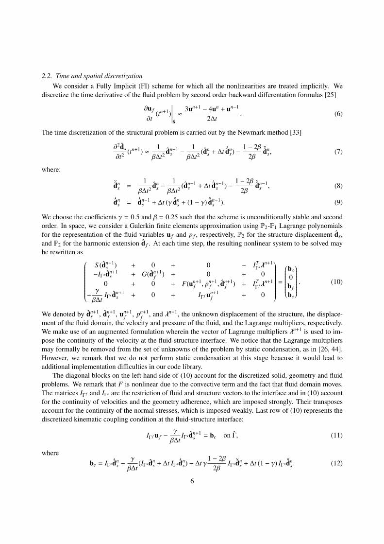
2.2. Time and spatial discretizationWe consider a Fully Implicit (FI) scheme for which all the nonlinearities are treated implicitly. We

discretize the time derivative of the fluid problem by second order backward differentation formulas [25]

∂u f

∂t(tn+1)

∣∣∣∣∣∣x ≈ 3un+1 − 4un + un−1

2∆t. (6)

The time discretization of the structural problem is carried out by the Newmark method [33]

∂2ds

∂t2 (tn+1) ≈1

β∆t2 dn+1s −

1β∆t2 (dn

s + ∆t ˙dns) −

1 − 2β2β

¨dns , (7)

where:

¨dns =

1β∆t2 dn

s −1

β∆t2 (dn−1s + ∆t ˙dn−1

s ) −1 − 2β

2β¨dn−1

s , (8)

˙dns = ˙dn−1

s + ∆t (γ ¨dns + (1 − γ) ¨dn−1

s ). (9)

We choose the coefficients γ = 0.5 and β = 0.25 such that the scheme is unconditionally stable and secondorder. In space, we consider a Galerkin finite elements approximation using P2-P1 Lagrange polynomialsfor the representation of the fluid variables u f and p f , respectively, P2 for the structure displacement ds,and P2 for the harmonic extension d f . At each time step, the resulting nonlinear system to be solved maybe rewritten as

S (dn+1s ) + 0 + 0 − IT

Γsλn+1

−IΓs dn+1s + G(dn+1

f ) + 0 + 00 + 0 + F(un+1

f , pn+1f , dn+1

f ) + ITΓ f λ

n+1

−γ

β∆tIΓs dn+1

s + 0 + IΓ f un+1f + 0

=

bs

0b f

bc

. (10)

We denoted by dn+1s , dn+1

f , un+1f , pn+1

f , and λn+1, the unknown displacement of the structure, the displace-ment of the fluid domain, the velocity and pressure of the fluid, and the Lagrange multipliers, respectively.We make use of an augmented formulation wherein the vector of Lagrange multipliers λn+1 is used to im-pose the continuity of the velocity at the fluid-structure interface. We notice that the Lagrange multipliersmay formally be removed from the set of unknowns of the problem by static condensation, as in [26, 44].However, we remark that we do not perform static condensation at this stage beacuse it would lead toadditional implementation difficulties in our code library.

The diagonal blocks on the left hand side of (10) account for the discretized solid, geometry and fluidproblems. We remark that F is nonlinear due to the convective term and the fact that fluid domain moves.The matrices IΓ f and IΓs are the restriction of fluid and structure vectors to the interface and in (10) accountfor the continuity of velocities and the geometry adherence, which are imposed strongly. Their transposesaccount for the continuity of the normal stresses, which is imposed weakly. Last row of (10) represents thediscretized kinematic coupling condition at the fluid-structure interface:

IΓ f u f −γ

β∆tIΓs dn+1

s = bc on Γ, (11)

wherebc = IΓs

˙dns −

γ

β∆t(IΓs dn

s + ∆t IΓs˙dn

s) − ∆t γ1 − 2β

2βIΓs

¨dns + ∆t (1 − γ) IΓs

¨dns . (12)

6

3. Numerical solution

We solve the nonlinear fully coupled FSI problem (10) using the Newton method as in, e.g., [23, 56, 31,10, 8]. Let us denote the solution of (10) at time tn = n ∆t by Xn = (dn

s , dnf ,u

nf , pn

f , λn)T . At each timestep, we

compute a sequence of approximations Xn+11 , Xn+1

2 , etc. until the numerical solution converges up to a pre-scribed tolerance. The generic k + 1 iteration of the Newton method applied to (10) is described as follows.Starting from an approximation of Xn+1

k , we compute the residual Rn+1k = (rn+1

ds,k, rn+1d f ,k, r

n+1u f ,k, r

n+1p f ,k, r

n+1λ,k )T :

Rn+1k =

bs

0b f

bc

−

S (dn+1s,k ) − IT

Γsλn+1k

−IΓs dn+1s,k + G(dn+1

f ,k )F(un+1

f ,k , pn+1f ,k , d

n+1f ,k ) + IT

Γ f λn+1k

−γ

β∆tIΓs dn+1

s,k + IΓ f un+1f ,k

. (13)

Then, we compute the Newton correction vector δXn+1k = (δdn+1

s,k , δdn+1f ,k , δu

n+1f ,k , δpn+1

f ,k , δλn+1k )T by solving

the Jacobian linear systemJFS I δXn+1

k = −Rn+1k , (14)

being

JFS I =

S 0 0 −IT

Γs

−IΓs G 0 00 D F IT

Γ f

−γ

β∆tIΓs 0 IΓ f 0

, (15)

where S, G and F represents the linearized structure, geometry and fluid problems, respectively;D are theshape derivatives, i.e. the derivatives of F(un+1

f , pn+1f , dn+1

f ) with respect to dn+1f (for their exact computation

see [23]).Finally, we update the solution: Xn+1

k+1 = Xn+1k + δXn+1

k . We stop the Newton iterations when

‖Rn+1k ‖∞

‖Rn+10 ‖∞

≤ ε, (16)

where Rn+10 is the residual at the first Newton iteration and ε is a given tolerance.

4. Preconditioning strategy

In analogy with what is proposed in [14], we exploit the block structure of the Jacobian matrix associatedto the fully coupled FSI problem (10) to build our preconditioner:

JFS I =

S 0−IΓs G

0 −ITΓs

0 00 D

−γ

β∆tIΓs 0

F ITΓ f

IΓ f 0

,

7

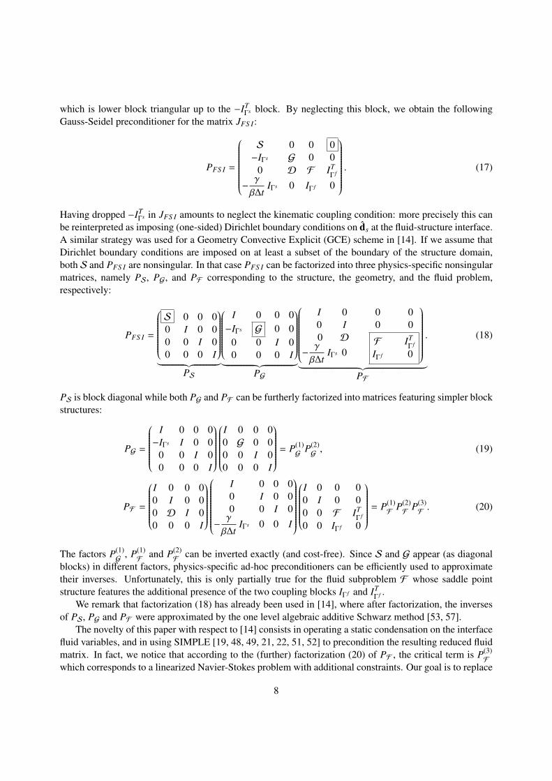
which is lower block triangular up to the −ITΓs block. By neglecting this block, we obtain the following

Gauss-Seidel preconditioner for the matrix JFS I:

PFS I =

S 0 0 0−IΓs G 0 0

0 D F ITΓ f

−γ

β∆tIΓs 0 IΓ f 0

. (17)

Having dropped −ITΓs in JFS I amounts to neglect the kinematic coupling condition: more precisely this can

be reinterpreted as imposing (one-sided) Dirichlet boundary conditions on ds at the fluid-structure interface.A similar strategy was used for a Geometry Convective Explicit (GCE) scheme in [14]. If we assume thatDirichlet boundary conditions are imposed on at least a subset of the boundary of the structure domain,both S and PFS I are nonsingular. In that case PFS I can be factorized into three physics-specific nonsingularmatrices, namely PS, PG, and PF corresponding to the structure, the geometry, and the fluid problem,respectively:

PFS I =

S 0 0 00 I 0 00 0 I 00 0 0 I

︸ ︷︷ ︸PS

I 0 0 0−IΓs G 0 0

0 0 I 00 0 0 I

︸ ︷︷ ︸PG

I 00 I

0 00 0

0 D

−γ

β∆tIΓs 0

F ITΓ f

IΓ f 0

.︸ ︷︷ ︸PF

(18)

PS is block diagonal while both PG and PF can be furtherly factorized into matrices featuring simpler blockstructures:

PG =

I 0 0 0−IΓs I 0 0

0 0 I 00 0 0 I

I 0 0 00 G 0 00 0 I 00 0 0 I

= P(1)G

P(2)G, (19)

PF =

I 0 0 00 I 0 00 D I 00 0 0 I

I 0 0 00 I 0 00 0 I 0

−γ

β∆tIΓs 0 0 I

I 0 0 00 I 0 00 0 F IT

Γ f

0 0 IΓ f 0

= P(1)F

P(2)F

P(3)F. (20)

The factors P(1)G

, P(1)F

and P(2)F

can be inverted exactly (and cost-free). Since S and G appear (as diagonalblocks) in different factors, physics-specific ad-hoc preconditioners can be efficiently used to approximatetheir inverses. Unfortunately, this is only partially true for the fluid subproblem F whose saddle pointstructure features the additional presence of the two coupling blocks IΓ f and IT

Γ f .We remark that factorization (18) has already been used in [14], where after factorization, the inverses

of PS, PG and PF were approximated by the one level algebraic additive Schwarz method [53, 57].The novelty of this paper with respect to [14] consists in operating a static condensation on the interface

fluid variables, and in using SIMPLE [19, 48, 49, 21, 22, 51, 52] to precondition the resulting reduced fluidmatrix. In fact, we notice that according to the (further) factorization (20) of PF , the critical term is P(3)

F

which corresponds to a linearized Navier-Stokes problem with additional constraints. Our goal is to replace

8

it, after static condensation of the interface variables, by a convenient approximation built on an efficientSIMPLE preconditioner.

We point out that our static condensation of the interface variables is operated at the level of the fluidpreconditioner. A different approach, see e.g. [26, 44], consists in removing the interface variables directlyfrom the set of unknowns of the FSI problem (14). In Section 4.2 we will show that the corresponding blockpreconditioner introduced in [26] differs from ours.

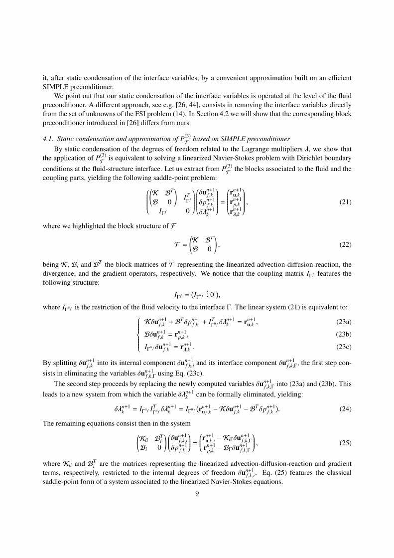
4.1. Static condensation and approximation of P(3)F

based on SIMPLE preconditionerBy static condensation of the degrees of freedom related to the Lagrange multipliers λ, we show that

the application of P(3)F

is equivalent to solving a linearized Navier-Stokes problem with Dirichlet boundaryconditions at the fluid-structure interface. Let us extract from P(3)

Fthe blocks associated to the fluid and the

coupling parts, yielding the following saddle-point problem:(K BT

B 0

)ITΓ f

IΓ f 0

δun+1

f ,kδpn+1

f ,kδλn+1

k

=

rn+1

u,krn+1

p,krn+1λ,k

, (21)

where we highlighted the block structure of F

F =

(K BT

B 0

), (22)

being K , B, and BT the block matrices of F representing the linearized advection-diffusion-reaction, thedivergence, and the gradient operators, respectively. We notice that the coupling matrix IΓ f features thefollowing structure:

IΓ f =(IΓ

u f... 0

),

where IΓu f is the restriction of the fluid velocity to the interface Γ. The linear system (21) is equivalent to:

Kδun+1f ,k + BTδpn+1

f ,k + ITΓ

u f δλn+1k = rn+1

u,k , (23a)

Bδun+1f ,k = rn+1

p,k , (23b)

IΓu f δun+1

f ,k = rn+1λ,k . (23c)

By splitting δun+1f ,k into its internal component δun+1

f ,k,i and its interface component δun+1f ,k,Γ, the first step con-

sists in eliminating the variables δun+1f ,k,Γ using Eq. (23c).

The second step proceeds by replacing the newly computed variables δun+1f ,k,Γ into (23a) and (23b). This

leads to a new system from which the variable δλn+1k can be formally eliminated, yielding:

δλn+1k = IΓ

u f ITΓ

u f δλn+1k = IΓ

u f(rn+1

u f ,k − Kδun+1f ,k − B

Tδpn+1f ,k

). (24)

The remaining equations consist then in the system(Kii B

Ti

Bi 0

) δun+1f ,k,i

δpn+1f ,k

=

rn+1u,k,i − KiΓδun+1

f ,k,Γrn+1

p,k − BΓδun+1f ,k,Γ

, (25)

where Kii and BTi are the matrices representing the linearized advection-diffusion-reaction and gradient

terms, respectively, restricted to the internal degrees of freedom δun+1f ,k,i. Eq. (25) features the classical

saddle-point form of a system associated to the linearized Navier-Stokes equations.

9

At this point we replace the matrix in (25) by its approximation based on SIMPLE preconditioner

F F =

(Kii 0Bi −S

) (I D−1BT

i0 I

), (26)

where D is the diagonal of Kii, and S = BiD−1BTi the approximated Shur complement of (25). In the ap-

plication of FaCSI, the inverses of S, G, Kii and S are approximated by associated efficient preconditionersdenoted by HS, HG, HKii and HS , respectively, based, e.g., on domain decomposition or the multigridmethod. This concludes the construction of the preconditioner FaCSI for JFS I , which takes the followingfinal form:

PFaCS I = PapS· PapG· PapF, (27)

where:

PapS

=

HS 0 0 00 I 0 00 0 I 00 0 0 I

, PapG

=

I 0 0 0−IΓs HG 0 0

0 0 I 00 0 0 I

(28)

and

PapF

=

I 0 0 00 I 0 0

0 D

I 0 00 IΓ 00 0 I

000

−γ

β∆tIΓs 0

(0 0 0

)I

I 0 0 00 I 0 0

0 0

I 0 00 0 00 0 I

0IΓ

0

0 0

(0 IΓ 0

)I

I 0 0 00 I 0 0

0 0

HKii KiΓ 00 IΓ 0Bi BΓ −HS

0IΓ

0

0 0

(0 0 0

)I

I 0 0 00 I 0 0

0 0

I 0 D−1BTi

0 IΓ 00 0 I

0IΓ

0

0 0

(0 0 0

)I

I 0 0 00 I 0 0

0 0

I 0 00 IΓ 00 0 I

000

0 0

(KΓi KΓΓ BT

Γ

)I

. (29)

For the sake of clarity, we point out that, for a given residual r = (rds , rd f , ru f , rp f , rλ)T , the application

of our preconditioner amounts to solve PFaCS Iw = r, therefore involving the following steps:

1. Application of (PapS

)−1: wds = H−1S

rds .

2. Application of (PapG

)−1: wd f = H−1G

(rd f + IΓswds).

3. Application of (PapF

)−1: compute zF = rF − Dwd f and zλ = rλ +γ

β∆tIΓswds . Then, after denoting

by wu and wp, zu and zp the velocity and pressure components of wF and zF , respectively, thanks to(23c) we set zu,Γ = zλ. The application of the SIMPLE preconditioner involves:

a) yu,i = H−1Kii

(zu,i − KiΓzu,Γ),

b) wp = H−1S

(Biyu,i − zp + BΓzu,Γ),

10

c) wu = (wu,i,wu,Γ)T = (yu,i − D−1BTi wp, zu,Γ)T .

Finally, we compute wλ = IΓu f (zu − Kwu − B

T wp).

Remark 2. In [30] a similar factorization as in Eq. (18) was used, and a SIMPLE preconditioner wasexploited to directly approximate the factor P(3)

F. However, no static condensation was used to eliminate the

interface fluid variables, yielding therefore to a different preconditioner. In Section 5.2 we show that staticcondensation substancially increases the performance with respect to the version proposed in [30].

4.2. Comparison with other condensed formulations

In [26] the authors consider a condensed formulation of the coupled FSI problem for which the un-knowns are ds,i, d f ,i, u f and p f , being ds,i and d f ,i the structure and fluid mesh displacement associated tothe internal degrees of freedom, respectively. In particular, the vector of Lagrange multipliers is condensedinto the structural displacement unknowns at the interface. In our case λ is condensed into the fluid velocity.

The block Gauss-Seidel preconditioner proposed in [26] (see Eq. (43) in [26]) reads:

M =

Sii 0

(0 0

)0 Gii

(0 0

)(SΓi

0

) (DΓi

Dii

) (δSΓΓ + FΓΓ + δDΓΓ FΓi

FiΓ + δDiΓ Fii

) (30)

In (30) each block matrix (i.e. S, G, F and D) is split into its internal (index i) and interface (index Γ)components; δ is a factor which converts displacement into velocity.

By comparing (17) with (30) we observe that the two block preconditioners are different. More specifi-cally, the nature of the subproblems change: in (30) the structure bears a Dirichlet problem, the ALE is stillof Dirichlet type and decoupled from the structure, while the fluid is a Neumann problem. In FaCSI, thestructure bears a Neumann problem, the ALE is of Dirichlet type and it is coupled with the structure whilethe fluid is of Dirichlet type. Furthermore, we notice that due to the condensed formulation adopted in [26],we observe that the fluid block in (30) slightly differs from ours at the interface.

The aforemetioned differences may be summarized by stating that the block Gauss-Seidel precondi-tioner devised in [26] is of Neumann-Dirichlet type while FaCSI is of Dirichlet-Neumann type. In [18]a comparison of the performance of Dirichlet-Neumann, Neumann-Dirichlet and Neumann-Neumann pre-conditioners for the Steklov-Poincare formulation of the FSI problem was carried out. There, it was shownthat the Dirichlet-Neumann preconditioner was the most efficient in terms of requested both CPU time andlinear solver iterations.

5. Numerical results

We test our FSI preconditioner on two different test cases: the first is an FSI example in which westudy the fluid flow in a straight flexible tube, the second consists in the simulation of the hemodynamicsin a femoropopliteal bypass. We measure the weak and strong scalability of the proposed preconditioner,namely the wall time and iterations count.

The FSI problem is discretized by a Fully Implicit (FI) second order scheme in time and space. Theresulting nonlinear system is solved by the exact Newton method using tolerance ε = 10−6 in (16). We solvethe linearized problem at each Newton iteration by the right preconditioned GMRES method [54] whichis never restarted. Since in our case the matrices associated to the harmonic extension and the structure

11

are constant throughout the simulation, their preconditioners HS and HG are computed once and stored.Conversely, we recompute the preconditioner associated to the fluid problem, namelyHKii andHS , at eachNewton iteration. The initial guess for Newton is set to zero to guarantee a comparable iterations countfrom one timestep to another. In practice, better choices can be made, e.g., by taking as initial guess anextrapolation of the solutions at the previous time steps.

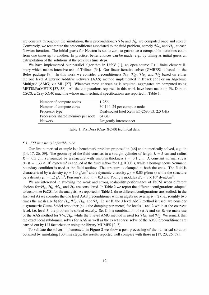
We have implemented our parallel algorithm in LifeV [1], an open-source C++ finite element li-brary which makes intensive use of Trilinos [34]. Our linear iterative solver (GMRES) is based on theBelos package [9]. In this work we consider preconditioners HS, HG, HKii and HS based on eitherthe one level Algebraic Additive Schwarz (AAS) method implemented in Ifpack [55] or on AlgebraicMultigrid (AMG) via ML [27]. Whenever mesh coarsening is required, aggregates are computed usingMETIS/ParMETIS [37, 38]. All the computations reported in this work have been made on Piz Dora atCSCS, a Cray XC40 machine whose main technical specifications are reported in Table 1.

Number of compute nodes 1’256Number of compute cores 30’144, 24 per compute nodeProcessor type Dual-socket Intel Xeon E5-2690 v3, 2.5 GHzProcessors shared memory per node 64 GBNetwork Dragonfly interconnect

Table 1: Piz Dora (Cray XC40) technical data.

5.1. FSI in a straight flexible tube

Our first numerical example is a benchmark problem proposed in [46] and numerically solved, e.g., in[14, 17, 26, 59]. The geometry of the fluid consists in a straight cylinder of length L = 5 cm and radiusR = 0.5 cm, surrounded by a structure with uniform thickness t = 0.1 cm. A constant normal stressσ · n = 1.33 × 104 dyne/cm2 is applied at the fluid inflow for t ≤ 0.003 s, while a homogeneous Neumannboundary condition is used at the fluid outflow. The structure is clamped at both the ends. The fluid ischaracterized by a density ρ f = 1.0 g/cm3 and a dynamic viscosity µ f = 0.03 g/(cm s) while the structureby a density ρs = 1.2 g/cm3, Poisson’s ratio νs = 0.3 and Young’s modulus Es = 3 × 106 dyne/cm2.

We are interested in studying the weak and strong scalability performance of FaCSI when differentchoices forHS,HG,HKii andHS are considered. In Table 2 we report the different configurations adoptedto customize FaCSI for the analysis. As reported in Table 2, three different configurations are studied: in thefirst (set A) we consider the one level AAS preconditioner with an algebraic overlap δ = 2 (i.e., roughly twotimes the mesh size h) for HS, HG, HKii and HS . In set B, the 3 level AMG method is used: we considera symmetric Gauss-Seidel smoother (ω is the damping parameter) for levels 1 and 2 while at the coarsestlevel, i.e. level 3, the problem is solved exactly. Set C is a combination of set A and set B: we make useof the AAS method for HS, HG, while the 3 level AMG method is used for HKii and HS . We remark thatthe exact local subdomain solves for AAS as well as the exact coarse solve of the AMG preconditioner arecarried out by LU factorization using the library MUMPS [2, 3].

To validate the solver implemented, in Figure 2 we show a post-processing of the numerical solutionobtained by simulating 100 time steps: the results reported well compare with those in [17, 23, 26, 59].

12

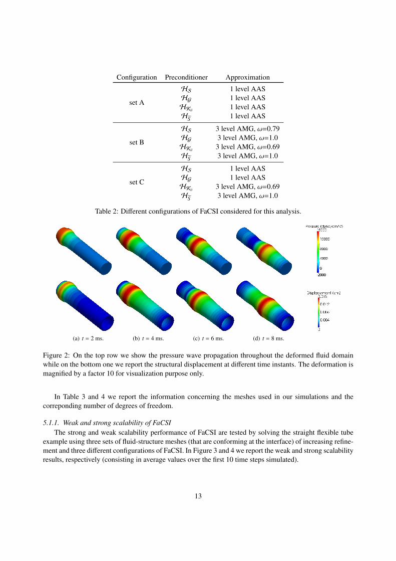
Configuration Preconditioner Approximation

set A

HS 1 level AASHG 1 level AASHKii 1 level AASHS 1 level AAS

set B

HS 3 level AMG, ω=0.79HG 3 level AMG, ω=1.0HKii 3 level AMG, ω=0.69HS 3 level AMG, ω=1.0

set C

HS 1 level AASHG 1 level AASHKii 3 level AMG, ω=0.69HS 3 level AMG, ω=1.0

Table 2: Different configurations of FaCSI considered for this analysis.

(a) t = 2 ms. (b) t = 4 ms. (c) t = 6 ms. (d) t = 8 ms.

Figure 2: On the top row we show the pressure wave propagation throughout the deformed fluid domainwhile on the bottom one we report the structural displacement at different time instants. The deformation ismagnified by a factor 10 for visualization purpose only.

In Table 3 and 4 we report the information concerning the meshes used in our simulations and thecorreponding number of degrees of freedom.

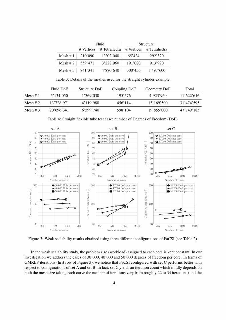
5.1.1. Weak and strong scalability of FaCSIThe strong and weak scalability performance of FaCSI are tested by solving the straight flexible tube

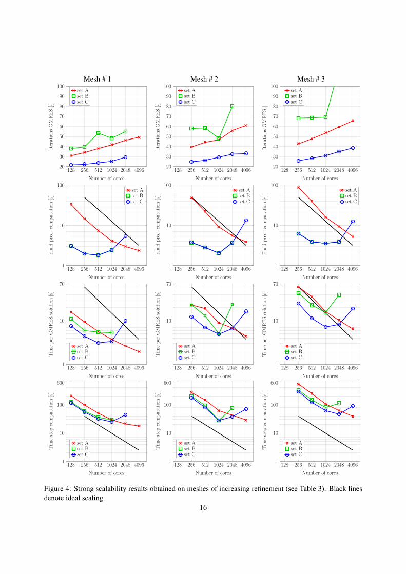
example using three sets of fluid-structure meshes (that are conforming at the interface) of increasing refine-ment and three different configurations of FaCSI. In Figure 3 and 4 we report the weak and strong scalabilityresults, respectively (consisting in average values over the first 10 time steps simulated).

13

Fluid Structure# Vertices # Tetrahedra # Vertices # Tetrahedra

Mesh # 1 210’090 1’202’040 65’424 292’320

Mesh # 2 559’471 3’228’960 191’080 913’920

Mesh # 3 841’341 4’880’640 300’456 1’497’600

Table 3: Details of the meshes used for the straight cylinder example.

Fluid DoF Structure DoF Coupling DoF Geometry DoF Total

Mesh # 1 5’134’050 1’369’030 195’576 4’923’960 11’622’616

Mesh # 2 13’728’971 4’119’980 456’114 13’169’500 31’474’595

Mesh # 3 20’696’341 6’599’740 598’104 19’855’000 47’749’185

Table 4: Straight flexible tube test case: number of Degrees of Freedom (DoF).

set A set B set C

256 512 1024 204820

30

40

50

60

70

80

90

100

Number of cores

IterationsGMRES[-]

30’000 Dofs per core40’000 Dofs per core50’000 Dofs per core

256 512 1024 204820

30

40

50

60

70

80

90

100

Number of cores

IterationsGMRES[-]

30’000 Dofs per core40’000 Dofs per core50’000 Dofs per core

256 512 1024 204820

30

40

50

60

70

80

90

100

Number of cores

IterationsGMRES[-]

30’000 Dofs per core40’000 Dofs per core50’000 Dofs per core

256 512 1024 204830

100

300

Number of cores

Tim

estep

computation

[s]

30’000 Dofs per core40’000 Dofs per core50’000 Dofs per core

256 512 1024 204830

100

300

Number of cores

Tim

estep

computation

[s]

30’000 Dofs per core40’000 Dofs per core50’000 Dofs per core

256 512 1024 204830

100

300

Number of cores

Tim

estep

computation

[s]

30’000 Dofs per core40’000 Dofs per core50’000 Dofs per core

Figure 3: Weak scalability results obtained using three different configurations of FaCSI (see Table 2).

In the weak scalability study, the problem size (workload) assigned to each core is kept constant. In ourinvestigation we address the cases of 30’000, 40’000 and 50’000 degrees of freedom per core. In terms ofGMRES iterations (first row of Figure 3), we notice that FaCSI configured with set C performs better withrespect to configurations of set A and set B. In fact, set C yields an iteration count which mildly depends onboth the mesh size (along each curve the number of iterations vary from roughly 22 to 34 iterations) and the

14

number of degrees of freedom per core since the three curves almost overlap. Configuration of set A leads toa number of linear iterations which on the one hand mildly depends on the core workload but on the other israther sensitive to the mesh size (along each curve the iterations vary from roughly 30 to 60 iterations). Weobserve that FaCSI configured with set B yields iteration counts that are affected by both the mesh size andthe number of degrees of freedom per core. We focus now on the weak scalability of the time to compute asingle time step (second row of Figure 3). FaCSI configured with set A leads to computational times that areweakly scalable for all the core workloads taken into account. Nevertheless, comparing the results obtainedby set A with those generated with set B and C, we notice that set A is the most computational expensive. Inparticular, we highlight that the time to compute a time step using set C with 50’000 Dofs per core (which isroughly 70 s) is smaller than the one with workload 30’000 Dofs per core using set A (that is roughly 80 s).FaCSI configured with set B is not weakly scalable as the timings obtained vary significantly (in particularwhen 30’000 Dofs per core are used). Using set C, we notice that the time to compute a single time step isweakly scalable for a core workload of 50’000 Dofs while for 30’000 and 40’000 it increases with the corescount as the time spent by communication is larger than the actual one associated to the relatively smallamount of computational work required on each individual core.

In Figure 4 we show the strong scalability results obtained. In the first row of Figure 4 we report thenumber of GMRES iterations, in the second row the time to build the preconditoner of the fluid problem, inthe third row the time to solve the linear system while in the fourth row the time to compute a single timestep. We remark that in the second row of Figure 4 we report the time to build only the preconditioner forthe fluid problem: in fact, since the harmonic extension and the structure matrices are constant throughoutthe simulation, their preconditioners are built only once and stored at the beginning.

In terms of linear solver iterations we notice that FaCSI configured with set C performs better than bothset A and set B (in line with what we observed in the study of the weak scalability). Indeed, for all the 3meshes considered, we notice that the use of set C leads to a number of linear solver iterations that is thelowest and which is less affected by the number of cores utilized.

Regarding the time to build the fluid preconditioner, although set A leads to strongly scalable results (the red curve behaves almost as the black one of the ideal scaling), we notice that up to 2’048 cores set B andset C allows for a remarkably faster computation w.r.t. set A. For instance, when a small number of coresis used, the construction of the fluid preconditioner by the algebraic multigrid method (set B and set C) isroughly ten times lower then the one of the overlapping algebraic additive Schwarz (set A). Nevertheless,although AMG leads to a very fast construction of the preconditioner, we notice that in our numericalexperiments its construction scales up to 512 cores (on Mesh # 3). We remark that the curves in the secondrow of Figure 4 associated to set B and set C are overlapping since their settings for the fluid problem are thesame (see Table 2). In terms of time to solve the linear system, we notice that with the configurations of setA FaCSI scales up to 2’048 cores, with set B until 512 cores whereas using set C linear scaling is obtainedup to 1’024 cores. It is noteworthy that until 1’024 cores the solution of the linear system carried out byFaCSI customized by set C is the fastest (in particular almost two times faster than set A). The last row ofFigure 4 shows the strong scalability of the time to compute a single time step. Strong scalability of FaCSIcustomized with set A, set B and set C is observed up to 4’096, 1’024 and 2’048 cores, respectively. Alsoin this case we notice that until FaCSI configured with set C scales linearly, it is the fastest. For instance,until 2’048 cores on Mesh # 3, we remark that the computational times associated to set A are roughly thesame of those obtained by set C using, for the latter, half of the cores.

Based on the analysis presented so far we conclude that FaCSI customized with set C (i.e. using theone level AAS method for both HS and HG, and the 3 level AMG method for HKii and HS ) is the mostcomputationally efficient and robust with respect to the mesh size among all the configurations taken into

15

Mesh # 1 Mesh # 2 Mesh # 3

128 256 512 1024 2048 409620

30

40

50

60

70

80

90

100

Number of cores

IterationsGMRES[-]

set Aset Bset C

128 256 512 1024 2048 409620

30

40

50

60

70

80

90

100

Number of cores

IterationsGMRES[-]

set Aset Bset C

128 256 512 1024 2048 409620

30

40

50

60

70

80

90

100

Number of cores

IterationsGMRES[-]

set Aset Bset C

128 256 512 1024 2048 40961

10

100

Number of cores

Fluid

prec.

computation

[s]

set Aset Bset C

128 256 512 1024 2048 40961

10

100

Number of cores

Fluid

prec.

computation

[s]

set Aset Bset C

128 256 512 1024 2048 40961

10

100

Number of cores

Fluid

prec.

computation

[s]

set Aset Bset C

128 256 512 1024 2048 40961

10

70

Number of cores

Tim

eper

GMRESsolution

[s]

set Aset Bset C

128 256 512 1024 2048 40961

10

70

Number of cores

Tim

eper

GMRESsolution

[s]

set Aset Bset C

128 256 512 1024 2048 40961

10

70

Number of cores

Tim

eper

GMRESsolution

[s]

set Aset Bset C

128 256 512 1024 2048 40961

10

100

600

Number of cores

Tim

estep

computation

[s]

set Aset Bset C

128 256 512 1024 2048 40961

10

100

600

Number of cores

Tim

estep

computation

[s]

set Aset Bset C

128 256 512 1024 2048 40961

10

100

600

Number of cores

Tim

estep

computation

[s]

set Aset Bset C

Figure 4: Strong scalability results obtained on meshes of increasing refinement (see Table 3). Black linesdenote ideal scaling.

16

account in our analysis.

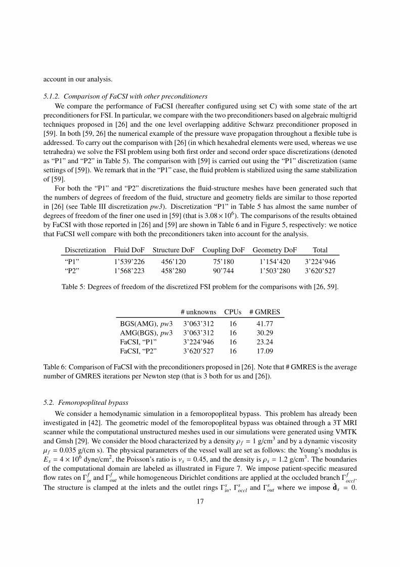
5.1.2. Comparison of FaCSI with other preconditionersWe compare the performance of FaCSI (hereafter configured using set C) with some state of the art

preconditioners for FSI. In particular, we compare with the two preconditioners based on algebraic multigridtechniques proposed in [26] and the one level overlapping additive Schwarz preconditioner proposed in[59]. In both [59, 26] the numerical example of the pressure wave propagation throughout a flexible tube isaddressed. To carry out the comparison with [26] (in which hexahedral elements were used, whereas we usetetrahedra) we solve the FSI problem using both first order and second order space discretizations (denotedas “P1” and “P2” in Table 5). The comparison with [59] is carried out using the “P1” discretization (samesettings of [59]). We remark that in the “P1” case, the fluid problem is stabilized using the same stabilizationof [59].

For both the “P1” and “P2” discretizations the fluid-structure meshes have been generated such thatthe numbers of degrees of freedom of the fluid, structure and geometry fields are similar to those reportedin [26] (see Table III discretization pw3). Discretization “P1” in Table 5 has almost the same number ofdegrees of freedom of the finer one used in [59] (that is 3.08×106). The comparisons of the results obtainedby FaCSI with those reported in [26] and [59] are shown in Table 6 and in Figure 5, respectively: we noticethat FaCSI well compare with both the preconditioners taken into account for the analysis.

Discretization Fluid DoF Structure DoF Coupling DoF Geometry DoF Total

“P1” 1’539’226 456’120 75’180 1’154’420 3’224’946“P2” 1’568’223 458’280 90’744 1’503’280 3’620’527

Table 5: Degrees of freedom of the discretized FSI problem for the comparisons with [26, 59].

# unknowns CPUs # GMRES

BGS(AMG), pw3 3’063’312 16 41.77AMG(BGS), pw3 3’063’312 16 30.29FaCSI, “P1” 3’224’946 16 23.24FaCSI, “P2” 3’620’527 16 17.09

Table 6: Comparison of FaCSI with the preconditioners proposed in [26]. Note that # GMRES is the averagenumber of GMRES iterations per Newton step (that is 3 both for us and [26]).

5.2. Femoropopliteal bypass

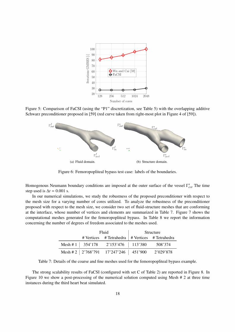
We consider a hemodynamic simulation in a femoropopliteal bypass. This problem has already beeninvestigated in [42]. The geometric model of the femoropopliteal bypass was obtained through a 3T MRIscanner while the computational unstructured meshes used in our simulations were generated using VMTKand Gmsh [29]. We consider the blood characterized by a density ρ f = 1 g/cm3 and by a dynamic viscosityµ f = 0.035 g/(cm s). The physical parameters of the vessel wall are set as follows: the Young’s modulus isEs = 4 × 106 dyne/cm2, the Poisson’s ratio is νs = 0.45, and the density is ρs = 1.2 g/cm3. The boundariesof the computational domain are labeled as illustrated in Figure 7. We impose patient-specific measuredflow rates on Γ

fin and Γ

fout while homogeneous Dirichlet conditions are applied at the occluded branch Γ

foccl.

The structure is clamped at the inlets and the outlet rings Γsin, Γs

occl and Γsout where we impose ds = 0.

17

128 256 512 1024 204820

30

40

50

60

70

80

90

100

Number of cores

IterationsGMRES[-]

Wu and Cai [59]FaCSI

Figure 5: Comparison of FaCSI (using the “P1” discretization, see Table 5) with the overlapping additiveSchwarz preconditioner proposed in [59] (red curve taken from right-most plot in Figure 4 of [59]).

Γfin

Γfoccl

Γfout

(a) Fluid domain.

Γsin

Γsoccl

ΓsoutΓsext

(b) Structure domain.

Figure 6: Femoropopliteal bypass test case: labels of the boundaries.

Homogenous Neumann boundary conditions are imposed at the outer surface of the vessel Γsext The time

step used is ∆t = 0.001 s.In our numerical simulations, we study the robustness of the proposed preconditioner with respect to

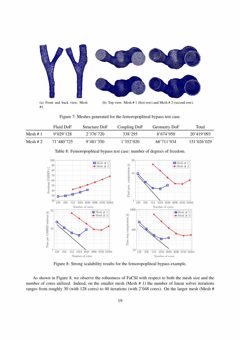
the mesh size for a varying number of cores utilized. To analyze the robustness of the preconditionerproposed with respect to the mesh size, we consider two set of fluid-structure meshes that are conformingat the interface, whose number of vertices and elements are summarized in Table 7. Figure 7 shows thecomputational meshes generated for the femoropopliteal bypass. In Table 8 we report the informationconcerning the number of degrees of freedom associated to the meshes used.

Fluid Structure# Vertices # Tetrahedra # Vertices # Tetrahedra

Mesh # 1 354’178 2’153’476 113’380 508’374

Mesh # 2 2’768’791 17’247’246 451’900 2’029’878

Table 7: Details of the coarse and fine meshes used for the femoropopliteal bypass example.

The strong scalability results of FaCSI (configured with set C of Table 2) are reported in Figure 8. InFigure 10 we show a post-processing of the numerical solution computed using Mesh # 2 at three timeinstances during the third heart beat simulated.

18

(a) Front and back view, Mesh#1.

(b) Top view: Mesh # 1 (first row) and Mesh # 2 (second row).

Figure 7: Meshes generated for the femoropopliteal bypass test case.

Fluid DoF Structure DoF Coupling DoF Geometry DoF Total

Mesh # 1 9’029’128 2’376’720 338’295 8’674’950 20’419’093

Mesh # 2 71’480’725 9’481’350 1’352’020 68’711’934 151’026’029

Table 8: Femoropopliteal bypass test case: number of degrees of freedom.

128 256 512 1024 2048 4096 8192 1638420

30

40

50

60

70

80

90

100

Number of cores

IterationsGMRES[-]

Mesh # 1Mesh # 2

128 256 512 1024 2048 4096 8192 163841

10

30

Number of cores

Fluid

prec.

computation

[s] Mesh # 1Mesh # 2

128 256 512 1024 2048 4096 8192 163841

10

70

Number of cores

Tim

eper

GMRESsolution

[s] Mesh # 1

Mesh # 2

128 256 512 1024 2048 4096 8192 1638410

100

1000

Number of cores

Tim

estep

computation

[s] Mesh # 1

Mesh # 2

Figure 8: Strong scalability results for the femoropopliteal bypass example.

As shown in Figure 8, we observe the robustness of FaCSI with respect to both the mesh size and thenumber of cores utilized. Indeed, on the smaller mesh (Mesh # 1) the number of linear solver iterationsranges from roughly 30 (with 128 cores) to 40 iterations (with 2’048 cores). On the larger mesh (Mesh #

19

2) the GMRES iterations increase from roughly 40 (using 512 cores) to 70 (with 16’384 cores). On thesmaller mesh the strong scalability of the time to compute a single time step is close to the ideal scaling upto 512 cores while on the larger mesh is close to the be linear until 4’096 cores. We observe that on bothMesh # 1 and Mesh # 2, FaCSI scales almost linearly until the local number of degrees of freedom per coreis roughly 40’000. For instance, on Mesh # 1 using 512 cores and on Mesh # 2 using 4’096 cores the singlecore workload is approximately 40’000. When the number of degrees of freedom per core is lower than40’000 the communication occurring for the construction of the preconditioner and the solution of the linearsystem (as shown in Figure 8) dominates the relatively small amount of computational work performed byeach single core. This behavior is in line with the weak scalability results obtained in Section 5.1.1 (seeFigure 3), where we observed that FaCSI (configured by set C) was weakly scalable up to 40’000 degreesof freedom per core.

We recall that in [30] a similar factorization as in Eq. (18) was used, and a SIMPLE preconditioner wasexploited to directly approximate the factor P(3)

F. However, no static condensation was used to eliminate the

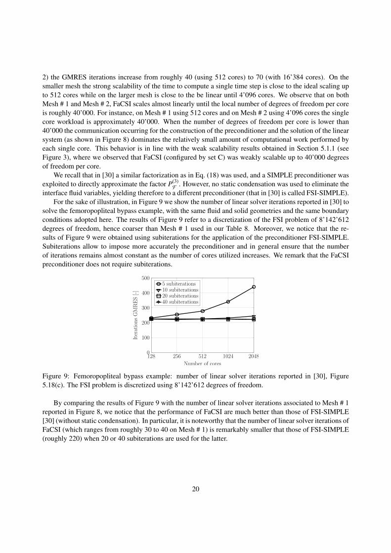
interface fluid variables, yielding therefore to a different preconditioner (that in [30] is called FSI-SIMPLE).For the sake of illustration, in Figure 9 we show the number of linear solver iterations reported in [30] to

solve the femoropopliteal bypass example, with the same fluid and solid geometries and the same boundaryconditions adopted here. The results of Figure 9 refer to a discretization of the FSI problem of 8’142’612degrees of freedom, hence coarser than Mesh # 1 used in our Table 8. Moreover, we notice that the re-sults of Figure 9 were obtained using subiterations for the application of the preconditioner FSI-SIMPLE.Subiterations allow to impose more accurately the preconditioner and in general ensure that the numberof iterations remains almost constant as the number of cores utilized increases. We remark that the FaCSIpreconditioner does not require subiterations.

128 256 512 1024 20480

100

200

300

400

500

Number of cores

IterationsGMRES[-]

5 subiterations10 subiterations20 subiterations40 subiterations

Figure 9: Femoropopliteal bypass example: number of linear solver iterations reported in [30], Figure5.18(c). The FSI problem is discretized using 8’142’612 degrees of freedom.

By comparing the results of Figure 9 with the number of linear solver iterations associated to Mesh # 1reported in Figure 8, we notice that the performance of FaCSI are much better than those of FSI-SIMPLE[30] (without static condensation). In particular, it is noteworthy that the number of linear solver iterations ofFaCSI (which ranges from roughly 30 to 40 on Mesh # 1) is remarkably smaller that those of FSI-SIMPLE(roughly 220) when 20 or 40 subiterations are used for the latter.

20

Figure 10: Post-processing of the results at time t = 1.8 s (left), 1.9 s (middle) and 2.0 s (right). Time t = 1.8s coincides with the systolic peak of the third heart beat simulated. In the top row we show the streamlinesof the fluid flow, in the middle row the magnitude of the structural displacement while in the bottom rowthe Wall Shear Stress.

21

6. Conclusion

We proposed a block preconditioner for FSI simulations that takes advantage of physics-specific ad-hocpreconditioners available for each subproblem (structure, geometry and fluid). We considered a secondorder discretization scheme in space and time and we solved the FSI problem using a monolithic couplingscheme wherein the nonlinearities are treated fully-implicitly. An analysis of the strong and weak scalabilityproperties of FaCSI was carried out by using different preconditioners (additive Schwarz and multigrid) forthe structure, geometry and fluid problems. Our analysis shows that the the most efficient choice consistsin using the 1 level algebraic additive Schwarz preconditioners for the structure and geometry problems,together with the 3 level algebraic multigrid method for the fluid. We tested the efficiency of the proposedblock preconditioner on a benchmark cylindrical configuration and on a realistic geometry of hemodynam-ics. We showed that FaCSI compares succesfully with state of the art preconditioners for FSI. Our parallelalgorithm showed scalability up to thousands of cores utilized on realistic problems where about 150 mil-lions of degrees of freedom were used, featuring also robustness with respect to mesh size.

Acknowledgements

We acknowledge the Swiss Platform for High-Performance and High-Productivity Computing (HP2C).The research of D. Forti was supported by the Swiss National Foundation (SNF), project no. 140184. Wegratefully acknowledge the CSCS for providing us the CPU resources under project ID s635. We acknowl-egde the Center for Advanced Modelling Science (CADMOS) for the use of the Lemanicus Blue Gene/Qsupercomputer. We also thank the LifeV community.

References

[1] LifeV user manual. http://www.lifev.org, 2010.[2] P. R. Amestoy, I. S. Duff, J. Koster, J. Y. L’Excellent. A fully asynchronous multifrontal solver using distributed dynamic

scheduling. SIAM J. Matrix Anal. Appl., 23(1):15–41, 2001.[3] P. R. Amestoy, A. Guermouche, J. Y. L’Excellent, S. Pralet. Hybrid scheduling for the parallel solution of linear systems.

Parallel Comput., 32(2), 136–156, 2006.[4] S. Badia, F. Nobile, and C. Vergara. Fluid-structure partitioned procedures based on Robin transmission conditions. J.

Comput. Phys., 227(14):7027–7051, 2008.[5] S. Badia, F. Nobile, and C. Vergara. Robin-Robin preconditioned Krylov methods for fluid-structure interaction problems.

Comput. Methods Appl. Mech. Engrg., 198(33-36):2768–2784, 2009.[6] S. Badia, A. Quaini, and A. Quarteroni. Modular vs. non-modular preconditioners for fluid-structure systems with large

added-mass effect. Comput. Methods Appl. Mech. Engrg., 197(49-50):4216–4232, 2008.[7] S. Badia, A. Quaini, and A. Quarteroni. Splitting methods based on algebraic factorization for fluid-structure interaction.

SIAM J. Sci. Comput., 30(4):1778–1805, 2008.[8] A. T. Barker and X.-C. Cai. Scalable parallel methods for monolithic coupling in fluid-structure interaction with application

to blood flow modeling. J. Comput. Phys., 229(3):642–659, 2010.[9] E. Bavier, M. Hoemmen, S. Rajamanickam, and H. Thornquist. Amesos2 and Belos: Direct and iterative solvers for large

sparse linear systems. Scientific Programming, 20(3):241–255, 2012.[10] Y. Bazilevs, V. M. Calo, T. J. R. Hughes, and Y. Zhang. Isogeometric fluid-structure interaction: theory, algorithms, and

computations. Comput. Mech., 43(1):3–37, 2008.[11] Y. Bazilevs, K. Takizawa, and T.E. Tezduyar. Computational Fluid–Structure Interaction. Methods and Applications. Wiley

Series in Computational Mechanics. Wiley, 2013.[12] P. Causin, J. F. Gerbeau, and F. Nobile. Added-mass effect in the design of partitioned algorithms for fluid-structure problems.

Comput. Methods Appl. Mech. Engrg., 194(42-44):4506–4527, 2005.[13] G. H. Cottet, E. Maitre, and T. Milcent. Eulerian formulation and level set models for incompressible fluid-structure interac-

tion. M2AN Math. Model. Numer. Anal., 42(3):471–492, 2008.

22

[14] P. Crosetto, S. Deparis, G. Fourestey, and A. Quarteroni. Parallel algorithms for fluid-structure interaction problems inhaemodynamics. SIAM J. Sci. Comput., 33(4):1598–1622, 2011.

[15] P. Crosetto, P. Reymond, S. Deparis, D. Kontaxakis, N. Stergiopulos, and A. Quarteroni. Fluid-structure interaction simulationof aortic blood flow. Comput. Fluids, 43:46–57, 2011.

[16] J. Degroote, K.-J. Bathe, and J. Vierendeels. Performance of a new partitioned procedure versus a monolithic procedure influidstructure interaction. Comput. Struct., 87:793–801, 2009.

[17] S. Deparis, M. Discacciati, G. Fourestey, and A. Quarteroni. Fluid-structure algorithms based on Steklov-Poincare operators.Comput. Methods Appl. Mech. Engrg., 195(41-43):5797–5812, 2006.

[18] S. Deparis, D. Forti, A. Heinlein, A. Klawonn, A. Quarteroni, and O. Rheinbach. A Comparison of Preconditioners for theSteklov-Poincare Formulation of the Fluid-Structure Coupling in Hemodynamics. PAMM, 15(1):93–94, 2015.

[19] S. Deparis, G. Grandperrin, and A. Quarteroni. Parallel preconditioners for the unsteady Navier–Stokes equations and appli-cations to hemodynamics simulations. Comput. Fluids, 92:253–273, 2013.

[20] W. G. Dettmer and D. Peric. A fully implicit computational strategy for strongly coupled fluidsolid interaction. Arch. Comput.Methods Engrg., 14(3):205–247, 2007.

[21] H. Elman, V. E. Howle, J. Shadid, R. Shuttleworth, and R. Tuminaro. Block preconditioners based on approximate commu-tators. SIAM J. Sci. Comput., 27(5):1651–1668, 2006.

[22] H. Elman, V. E. Howle, J. Shadid, R. Shuttleworth, and R. Tuminaro. A taxonomy and comparison of parallel block multi-level preconditioners for the incompressible Navier-Stokes equations. J. Comput. Phys., 227(3):1790–1808, 2008.

[23] M. A. Fernandez and M. Moubachir. A Newton method using exact jacobians for solving fluidstructure coupling. Comput.Struct., 83:127–142, 2005.

[24] L. Formaggia, A. Quarteroni, and A. Veneziani, editors. Cardiovascular mathematics, volume 1 of MS&A. Modeling, Simu-lation and Applications. Springer-Verlag Italia, Milan, 2009. Modeling and simulation of the circulatory system.

[25] D. Forti and L. Dede. Semi–implicit BDF time discretization of the Navier–Stokes equations with VMS–LES modeling inHigh Performance Computing framework. Comput. Fluids, 117:168–182, 2015.

[26] M. W. Gee, U. Kuttler and W. A. Wall. Truly monolithic algebraic multigrid for fluid-structure interaction. Int. J. Numer.Engng, 85:987–1016, 2011.

[27] M. W. Gee, C. M. Siefer, J. J. Hu, R. S. Tuminaro, and M. G. Sala. ML 5.0 Smoothed Aggregation User’s Guide, SandiaNational Laboratories, 2006.

[28] J. F. Gerbeau and M. Vidrascu. A quasi-Newton algorithm based on a reduced model for fluid-structure interaction problemsin blood flows. M2AN Math. Model. Numer. Anal., 37(4):631–647, 2003.

[29] C. Geuzaine and J. F. Remacle. Gmsh reference manual. Technical report, University of Liege, 2010.http://geuz.org/gmsh/doc/texinfo/gmsh.pdf.

[30] G. Grandperrin. Parallel Preconditioners for Navier-Stokes Equations and Fluid-Structure Interaction Problems: Applicationto Hemodynamics. PhD thesis, EPFL, 2013.

[31] M. Heil. An efficient solver for the fully coupled solution of large-displacement fluid–structure interaction problems. Comput.Methods Appl. Mech. Engrg., 193(1-2):1–23, 2004.

[32] M. Heil, A. L. Hazel, and J. Boyle. Solvers for large–displacement fluid–structure interaction problems: segregated versusmonolithic approaches. Comput. Mech., 43(1):91–101, 2008.

[33] T. J. R. Hughes. The finite element method: linear static and dynamic finite element analysis. Courier Corporation, 2012.[34] M. A. Heroux, R. A. Bartlett, V. E. Howle, R. J. Hoekstra, J. J. Hu, T. G. Kolda, R. B. Lehoucq, K. R. Long, R. P. Pawlowski,

E. T. Phipps, A. G. Salinger, H. K. Thornquist, R. S. Tuminaro, J. M. Willenbring, A. Williams, and K. S. Stanley. Anoverview of the trilinos project. ACM Trans. Math. Softw., 31(3):397–423, 2005.

[35] R. A. Horn and C. R. Johnson. Matrix Analysis. Cambridge University Press, 1990.[36] R. A. Horn and C. R. Johnson. Topics in matrix analysis. Cambridge University Press, Cambridge, 1991.[37] G. Karypis, K. Schloegel, and V. Kumar. METIS: A Software Package for Partitioning Unstructured Graphs, Partitioning

Meshes, and Computing Fill-Reducing Orderings of Sparse Matrices. Technical report, Univ MN., 1998.[38] G. Karypis, K. Schloegel, and V. Kumar. ParMETIS: Parallel Graph Partitioning and Sparse Matrix Ordering library. Tech-

nical report, Univ MN., 2003.[39] U. Kuttler, M. W. Gee, C. Forster, A. Comerford, and W. A. Wall. Coupling strategies for biomedical fluid-structure interac-

tion problems. Int. J. Numer. Methods Biomed. Eng., 26(3-4):305–321, 2010.[40] U. Kuttler and W. A. Wall. Fixed-point fluid–structure interaction solvers with dynamic relaxation. Comput. Mech., 43(1):61–

72, 2008.[41] P. Le Tallec and J. Mouro. Fluid structure interaction with large structural displacements. Comput. Methods Appl. Mech.

Engrg., 190:3039–3067, 2001.[42] E. Marchandise, P. Crosetto, C. Geuzaine, J. F. Remacle, and E. Sauvage. Quality open source mesh generation for cardio-

vascular flow simulations. In D. Ambrosi, A. Quarteroni, and G. Rozza, editors, Modeling of Physiological Flows, volume 5

23

of MS&A Modeling, Simulation and Applications, pages 395–414. Springer Milan, 2012.[43] H. G. Matthies, R. Niekamp, and J. Steindorf. Algorithms for strong coupling procedures. Comput. Methods Appl. Mech.

Engrg., 195(17-18):2028–2049, 2006.[44] M. Mayr, T. Kloppel, W. A. Wall, and M. W. Gee. A temporal consistent monolithic approach to fluid-structure interaction

enabling single field predictors. 2015. SIAM J. Sci. Comput., 37(1):B30–B59, 2015.[45] R. Mittal and G. Iaccarino. Immersed boundary methods. In Annual review of fluid mechanics. Vol. 37, volume 37 of Annu.

Rev. Fluid Mech., pages 239–261. Annual Reviews, Palo Alto, CA, 2005.[46] F. Nobile. Numerical approximation of fluid-structure interaction problems with application to haemodynamics. PhD thesis,

SB, Lausanne, 2001.[47] F. Nobile, M. Pozzoli, and C. Vergara. Inexact accurate partitioned algorithms for fluidstructure interaction problems with

finite elasticity in haemodynamics. J. Comput. Phys., 273(0):598 – 617, 2014.[48] S. V. Patankar and D. B. Spalding. A calculation procedure for heat, mass and momentum transfer in three dimensional

parabolic flows. Int. J. Heat Mass Transfer, 15:1787–1806, 1972.[49] M. Pernice and M. D. Tocci. A multigrid-preconditioned Newton-Krylov method for the incompressible Navier-Stokes

equations. SIAM J. Sci. Comput., 23(2):398–418 (electronic), 2001. Copper Mountain Conference (2000).[50] C. S. Peskin. The immersed boundary method. Acta Numer., 11:479–517, 2002.[51] M. Rehman, C. Vuik and G. Segal. SIMPLE-type preconditioners for the Oseen problem. Int. J. Num. Meth. in Fluids,

61:432–452, 2009.[52] M. Rehman, C. Vuik and G. Segal. Preconditioners for the steady incompressible Navier-Stokes problem. International

Journal of Applied Mathematics, 38:223–232, 2008.[53] A. Quarteroni and A. Valli. Domain decomposition methods for partial differential equations. Numerical Mathematics and

Scientific Computation. The Clarendon Press - Oxford University Press, New York, 1999. Oxford Science Publications.[54] Y. Saad and M. H. Schultz. GMRES: a generalized minimal residual algorithm for solving nonsymmetric linear systems.

SIAM J. Sci. Statist. Comput., 7(3):856–869, 1986.[55] M. Sala and M. Heroux. Robust Algebraic Preconditioners with IFPACK 3.0, Sandia National Laboratories, 2005.[56] T. E. Tezduyar, S. Sathe, and K. Stein. Solution techniques for the fully discretized equations in computation of fluid-structure

interactions with the space-time formulations. Comput. Methods Appl. Mech. Engrg., 195(41-43):5743–5753, 2006.[57] A. Toselli and O. Widlund. Domain decomposition methods—algorithms and theory, volume 34 of Springer Series in Com-

putational Mathematics. Springer-Verlag, Berlin, 2005.[58] H. Wang, J. Chessa, W. K. Liu, and T. Belytschko. The immersed/fictitious element method for fluid-structure interaction:

volumetric consistency, compressibility and thin members. Int. J. Numer. Meth. Eng., 74(1):32–55, 2008.[59] Y. Wu and X. C. Cai. A fully implicit domain decomposition based ALE framework for three-dimensional fluid-structure

interaction with application in blood flow computation. J. Comput. Phys., 258:524–537, 2014.

24

Recent publications:

MATHEMATICS INSTITUTE OF COMPUTATIONAL SCIENCE AND ENGINEERING Section of Mathematics

Ecole Polytechnique Fédérale CH-1015 Lausanne

01.2015 PENG CHEN, ALFIO QUARTERONI, GIANLUIGI ROZZA: Reduced order methods for uncertainty quantification problems 02.2015 FEDERICO NEGRI, ANDREA MANZONI, DAVID AMSALLEM: Efficient model reduction of parametrized systems by matrix discrete empirical

interpolation 03.2015 GIOVANNI MIGLIORATI, FABIO NOBILE, RAÚL TEMPONE: Convergence estimate in probability and in expectation for discrete least squares

with noisy evaluations at random points 04.2015 FABIO NOBILE, LORENZO TAMELLINI, FRANCESCO TESEI, RAÚL TEMPONE: An adaptive sparse grid alorithm for elliptic PDEs with lognormal diffusion

coefficent 05.2015 MICHAEL STEINLECHNER: Riemannian optimization for high-dimensional tensor completion 06.2015 V. R. KOSTIĆ, A. MIEDLAR, LJ. CVETKOVIĆ: An algorithm for computing minimal Geršgorin sets 07.2015 ANDREA BARTEZZAGHI, LUCA DEDÈ, ALFIO QUARTERONI: Isogeometric analysis of high order partial differential equations on surfaces 08.2015 IVAN FUMAGALLI, ANDREA MANZONI, NICOLA PAROLINI, MARCO VERANI: Reduced basis approximation and a posteriori error estimates for parametrized elliptic

eigenvalue problems 09.2015 DAVIDE FORTI, LUCA DEDÈ:

Semi-implicit BDF time discretization of the Navier-Stokes equations with VMS-LES modeling in a High Performance Computing framework

10.2015 PETAR SIRKOVIĆ, DANIEL KRESSNER: Subspace acceleration for large-scale parameter-dependent Hermitian

eigenproblems 11.2015 FEDERICO NEGRI: A model order reduction framework for parametrized nonlinear PDE-constrained

optimization 12.2015 ANNA TAGLIABUE, LUCA DEDÈ. ALFIO QUARTERONI: Nitsche’s method for parabolic partial differential equations with mixed time varying

boundary conditions 13.2015 NEW SIMONE DEPARIS, DAVIDE FORTI, GWENOL GRANDPERRIN, ALFIO QUARTERONI: FaCSI: A block parallel preconditioner for fluid-structure interaction in

hemodynamics