Electronic copy available at: https://ssrn.com/abstract=3116974

Factor momentum∗

Rob Arnott Mark Clements Vitali Kalesnik Juhani Linnainmaa†

January 2018

Abstract

Past industry returns predict the cross section of industry returns, and this predictability is

at its strongest at the one-month horizon (Moskowitz and Grinblatt 1999). We show that

the cross section of factor returns shares this property, and that industry momentum stems

from factor momentum. Factor momentum is transmitted into the cross section of industry

returns via variation in industries’ factor loadings. Momentum in industry-neutral factors spans

industry momentum; factor momentum is therefore not a by-product of industry momentum.

Factor momentum is a pervasive property of all factors; we show that factor momentum can be

captured by trading almost any set of factors. Factor momentum does not resolve the puzzle of

momentum in individual stock returns; it significantly deepens this puzzle.

∗Arnott, Clements, and Kalesnik are with Research Affiliates LLC. Linnainmaa is with the University of SouthernCalifornia and NBER.†Corresponding author. Mailing address: University of Southern California Marshall School of Business, 3670

Trousdale Pkwy, Los Angeles, CA 90089, United States. E-mail address: Juhani.Linnainmaa@Marshall.usc.edu.Telephone number: +1 (213) 821-9898.

Electronic copy available at: https://ssrn.com/abstract=3116974

1 Introduction

Industries exhibit return momentum similar to that found in the cross section of stock returns.

Moskowitz and Grinblatt (1999) show that this effect is at its strongest at the one-month horizon,

but that it lasts up to a year.1 Using data on 51 factors identified in the literature as significant

predictors of stock returns, we show that factor momentum is stronger than industry momentum

and that factor momentum fully subsumes industry momentum. The mechanism of transmission

is through differences in industries’ factor loadings. Industry returns are linear combinations of

factor returns. If the cross section of factor returns exhibit momentum, so will any nondegenerate

rotation of these factors as well.

The difficulty in testing the hypothesis that industry momentum stems from factor momentum

is in demonstrating the effect’s direction. Although industries can be written as rotations of factors,

factors could just as well be expressed as rotations of industries. If factors have incidental industry

exposures, industry return shocks impact factor returns via factors’ industry bets (Asness, Frazzini,

and Pedersen 2014). Factor momentum could thus be an expression of industry momentum and not

the other way around. We resolve this identification problem by utilizing industry-neutral factors.

We first sort stocks into portfolios by industry-demeaned return predictors; an industry-neutral

factor’s long and short sides are thus almost equally balanced across industries (Cohen and Polk

1996; Asness, Porter, and Stevens 2000). We then remove any remaining industry bets by taking

an offsetting position in each stock’s value-weighted industry (Novy-Marx 2013). These factors are

thereby, by construction, unrelated to past industry returns, and their future returns are orthogonal

to industry return shocks.

A strategy that rotates all 51 factors based on their prior one-month returns and holds them

for a month earns an annualized average return of 10.5% with a t-value of 5.01. A strategy that

1See, also, Grundy and Martin (2001), Lewellen (2002), and Hoberg and Phillips (2017) for analyses of industrymomentum.

1

uses industry-adjusted factors earns an average return of 6.4% with a t-value of 5.55. We show that

past returns on unadjusted factors contain no information about future returns once we control

for momentum in industry-adjusted factors. Similar to industry momentum, factor momentum is

at its strongest with one-month formation and holding periods. However, we also consider all 36

strategies that use formation and holding periods ranging from one to six months. Each strategy’s

Fama and French (2015) five-factor model alpha is statistically significant with a t-value of at least

3.25.

Momentum in industry-adjusted factors fully subsumes industry momentum. After controlling

for individual stock momentum and the five factors of the Fama and French (2015) model, an in-

dustry momentum strategy that uses one-month formation and holding periods earns an annualized

return of 8.6% (t-value = 4.09). However, controlling for factor momentum, also this strategy’s

alpha falls close to zero. Industry momentum, by contrast, does not subsume factor momentum.

When we control for individual stock momentum, industry momentum, and the five factors of the

Fama and French (2015) model, all factor momentum strategies that use formation and holding

periods ranging from one month to six months earn positive alphas. The strategy that stands out

in both economic and statistical significance is the one that rotates factors based on their prior

one-month returns and holds them for a month. This strategy’s alpha is 32 basis points per month

with a t-value of 3.85.

Factor momentum also subsumes momentum found in the returns of other well-diversified port-

folios. Lewellen (2002) shows that the 25 Fama and French (1993) portfolios sorted by size and

book-to-market exhibit cross-sectional momentum similar to industry momentum and that the

“size and B/M momentum is distinct from industry momentum in that neither subsumes the

other” (p. 534). Factor momentum subsumes both industry and size and book-to-market momen-

tum. The vector of transmission is plausibly the same as that for industries. If portfolios sorted by

size and book-to-market have different factor exposures, factor momentum bleeds into this cross

2

section of portfolio returns.

We show that our ability to explain industry momentum with factor momentum is not due to

a judicious choice of factors. Factor momentum is not due to any one factor; almost any set of

factors exhibits momentum. We first illustrate this result by considering the market, size, value,

investment, and profitability factors of the Fama and French (2015) five-factor model. A strategy

that is long the factor with the highest prior one-month return and short the one with the lowest

return earns an average annualized return of 8.0% with a t-value of 3.30. This strategy’s annualized

five-factor model alpha is even higher, 10.7% (t-value = 4.37). This strategy thus earns a high return

by rotating toward factors that are about to earn high returns and not by being consistently long

and short the factors with the highest and lowest premiums.2

We also construct random sets of factors that differ in size. The profitability of a strategy that

trades factor momentum using a random set of, say, ten factors is nearly the same as that of the

full set. In fact, a strategy that captures momentum in factor returns by rotating between just

two randomly selected factors is typically statistically significant as well! Factor momentum is also

robust to implementation restrictions. The effect remains significant even when the factors trade

only big stocks, or when we introduce a delay between the formation and holding periods.

We show that factor momentum’s abnormal returns are not specific to any one part of the 1963

through 2016 sample period. Whereas industry momentum “stops working” around year 2000,

post-2000 factor momentum is indistinguishable from pre-2000 momentum. Moreover, whereas

stock momentum suffers crashes (Barroso and Santa-Clara 2015; Daniel and Moskowitz 2016),

factor momentum experiences positive crashes. When stock momentum crashed at the onset of

market recovery in 2009, factor momentum generated sudden and outsized profits.

2This test is about the Conrad and Kaul (1998) mechanism. Conrad and Kaul note that “the repeated purchaseof winners from the proceeds of the sale of losers will, on average, be tantamount to the purchase of high-meansecurities from the sale of low-mean securities. Consequently, as long as there is some cross-sectional dispersion in themean returns of the universe of securities, a momentum strategy will be profitable.” The five-factor model regressionremoves the factor momentum strategy’s static exposures against the five factors; the remaining alpha must thereforeemerge from dynamic changes in factor weights.

3

Factors differ in their contributions to factor momentum profits. While the strategy that trades

the full set of 51 factors has an average return that is statistically significant with a t-value of

5.55, some combinations of factors generate momentum profits that have t-values in excess of 8.0.

We estimate a “momentum score” for each factor by measuring how much the factor momentum’s

profits suffer when we remove it from the set of factors being traded. The more important a factor,

the greater the resulting reduction in the strategy’s profits. We find that factors’ momentum scores

are asymmetric; some factors contribute significantly more towards factor momentum profits than

others, but no factor significantly lowers these profits. The factors that relate to distress, illiquidity,

and idiosyncratic risk are among those that contribute the most toward factor momentum profits.

The factors that display the most momentum are not the same as those with the highest mean

returns. At the very top of the list, for example, are firm age (Barry and Brown 1984) and nominal

stock price (Blume and Husic 1973) factors; both of these factors are, at best, weak predictors of

future returns in the 1963–2016 sample.

Both industry and factor momentum closely relate to short-term reversals of Jegadeesh (1990).

Whereas stock returns negatively predict the cross section of stock returns at the one-month horizon,

industries and factors both positively predict returns at this horizon. Short-term return reversals are

therefore an industry-relative effect; a stock’s return relative to the industry average is a significantly

more powerful predictor of returns than its raw return (Da, Liu, and Schaumburg 2013; Novy-Marx

and Velikov 2016). Indeed, whereas the five-factor plus momentum model alpha of the short-term

reversals factor is 6.1% per year (t-value = 3.61), this alpha increases to 10.2% (t-value = 8.44)

when we control industry momentum. If we also control for factor momentum, the alpha on short-

term reversals is 12.6% with a t-value of 12.85. It is therefore the stock’s return net of its industry

and factor exposures that negatively predicts returns. Factor momentum and short-term reversals

also significantly enhance the profitability of the individual stock momentum strategy. Whereas

UMD’s five-factor model alpha is 72 basis points per month (t-value = 4.31), this alpha increases to

4

136 basis points (t-value = 8.08) when the strategy has no exposures against short-term reversals

or factor momentum. Factor momentum is therefore not the cause of stock momentum; stock

momentum grows far stronger when we control for factor momentum.

Our results relate to Grundy and Martin (2001), who note that momentum strategies, by

the virtue of choosing stocks based on their past returns, have time-varying risk exposures. If a

factor earns a high return during a momentum strategy’s formation period, then winner stocks are

predominantly those that load positively on this factor. Kothari and Shanken (1992) and Daniel and

Moskowitz (2016) note that winners’ and losers’ market betas typically differ significantly through

this same mechanism. Grundy and Martin (2001) show that these incidental factor exposures do not

drive stock momentum profits; in fact, removing them enhances the profitability of stock momentum

strategies. Our result is that factor returns themselves exhibit cross-sectional momentum.

Our results also relate to Avramov, Cheng, Schreiber, and Shemer (2017) who extend the results

of Lewellen (2002) and show that momentum strategy also works for combinations of many well-

diversified portfolios. They sort stocks into portfolios by 15 return predictors, take the top and

bottom portfolios, and find strong cross-sectional momentum within this set of portfolios as well.

We find momentum in factor returns themselves, show that this form of momentum drives both

industry and size-and-B/M momentum, and show that factor momentum is present in almost all

factors.

2 Data

2.1 CRSP and Compustat

We use monthly and daily returns data on stocks listed on NYSE, AMEX, and Nasdaq from the

Center for Research in Securities Prices (CRSP). We include ordinary common shares (share codes

10 and 11) and use CRSP delisting returns. If a stock’s delisting return is missing and the delisting

5

is performance-related, we impute a return of −30% for NYSE and AMEX stocks (Shumway 1997)

and −55% for Nasdaq stocks (Shumway and Warther 1999).

We obtain accounting data from annual Compustat files to compute some of the return predic-

tors we detail in Section 2.2. We follow the standard convention and lag accounting information

by six months (Fama and French 1993). For example, if a firm’s fiscal year ends in December in

year t, we assume that this information is available to investors at the end of June in year t+ 1.

We compute returns on our factors from July 1963 through December 2016. Some of the

predictors that we use to form the factors—such as idiosyncratic volatility and market beta—

however, use some pre-1963 return data.

2.2 Universe of factors

Table 1 reports average returns and three- and five-factor model alphas for the 51 factors that

we examine throughout this study. These factors are among those examined in McLean and Pontiff

(2016) and Linnainmaa and Roberts (2017). In Table 1 we divide the factors into two groups.

Accounting-based predictors use some income statement or balance sheet information; return-based

predictors use return, price, or volume information.3

We construct each factor as an HML-like factor by sorting stocks into six portfolios by size and

return predictor. We use NYSE breakpoints—median for size and the 30th and 70th percentiles for

the return predictor—and use independent sorts in the two dimensions. The exceptions to this rule

are factors that use discrete signals. The high and low portfolios of the debt issuance factor, for

example, include firms that did not issue (high portfolio) or issued (low portfolio) debt during the

prior fiscal year. We compute value-weighted returns on the six portfolios. A factor’s return is the

average return on the two high portfolios minus that on the two low portfolios. In assigning stocks

to the high and low portfolios, we sign the return predictors so that the high portfolios contain

3We classify “size” as an accounting-based predictor because we construct it as in Fama and French (1993) bysorting stocks into portfolios by book-to-market and size.

6

those stocks that the original study identifies as earning higher average returns.4 We rebalance

accounting-based factors annually at the end of each June and the return-based factors monthly.

The left-hand side of Table 1 reports average returns, alphas, and t-values for the standard

factors; the right-hand side reports them for the industry-adjusted factors. Standard factors sort

stocks by unadjusted return predictors. In constructing the industry-adjusted factors, we first

demean the predictors by the 49 Fama-French industries. The long and short sides of each factor

are thus approximately evenly diversified across industries. We then hedge any remaining industry

bets by taking an offsetting position in each stock’s value-weighted industry; that is, if a factor

takes a long position in stock i, it also takes a short position of the same magnitude in stock

i’s industry. Past returns on these industry-adjusted factors are unrelated to industry returns

because of the demeaning step; and future industry returns do not affect factor returns because the

returns are industry-hedged. This definition of industry-adjusted factors is the same as that used

by Novy-Marx (2013).

The comparison between average returns and three-factor model alphas in Table 1 shows that

some factors perform significantly better when controlling for size and book-to-market. Gross

profitability of Novy-Marx (2013), for example, is a particularly strong return predictor when

holding book-to-market fixed. It earns an average return of just 21 basis points per month (t-value

= 2.35), but a three-factor model alpha of 38 basis points (t-value = 5.36).

A comparison of the standard and industry-adjusted factors shows that industry adjustment

often improves factor performance (Cohen and Polk 1996; Asness, Porter, and Stevens 2000; Novy-

4Blume and Husic (1973) show that nominal stock price negatively predicts returns of NYSE stocks between 1932and 1966; this relationship is statistically significantly up to 1955. Because of this finding in the original study, weassign low-priced stocks into the “high” portfolios. During our 1963–2016 sample period, the resulting factor earnsa negative average return and negative three- and five-factor model alphas. That is, nominal stock price positivelypredicts returns during our sample period. The leverage factor of Bhandari (1988) is another factor that displayssimilar behavior. Because the factor momentum strategies we consider assign factors into portfolios based on priorreturns, the way we sign the factors is inconsequential. For example, if low-priced stocks significantly outperformhigh-priced stocks, the factor momentum strategy proceeds to take long positions in low-priced stocks. It does notmatter whether we express the return on the factor as a positive or negative number.

7

Marx 2013), and sometimes dramatically so. The five-factor model alpha associated with short-term

reversals, for example, is 37 basis points (t-value = 3.02). The industry-adjusted factor’s alpha,

by contrast, is 74 basis points per month (t-value = 9.24). Out of the 47 factors that are not part

of the five-factor model, the t-values associated with the industry-adjusted factors are higher 38

times.

3 Factor and industry momentum

3.1 Factor momentum

A cross-sectional momentum strategy selects assets or portfolios of assets based on their relative

returns over some formation period. In the cross section of individual stocks, for example, the typical

strategy measures returns over the prior one-year period skipping a month, and assigns stocks into

portfolios monthly (Novy-Marx 2012). These strategies skip a month because individual stock

returns tend to reverse at the one-month horizon.

We follow Jegadeesh and Titman (1993) and Moskowitz and Grinblatt (1999) in defining the

factor momentum strategy. Each month we rank factors by their average returns over a prior

L month period, and then take long and short positions in the best and worst performers. The

strategy invests an equal amount in each factor in the strategy’s long and short sides. We then hold

this strategy over the following H months. Each strategy is therefore described by an L/H pair.

We also need to specify the number of factors in which the strategy takes positions. Moskowitz

and Grinblatt (1999) use 20 industry portfolios and take long and short positions in the top three

and bottom three industries. We follow this rule and let the factor momentum strategy take long

and short positions in

n = max

{round(

3

20×N), 1

}(1)

factors, where N is the number of factors. Our full set has 51 factors, but we later consider subsets

8

in which N ranges from 2 and 50.

When the holding period is longer than a month, H > 1, the holding-period returns overlap.

We use the Jegadeesh and Titman (1993) approach to restructure the data to address this overlap.

For example, when the holding period is H = 3 months, we form the factor momentum strategy

each month t and compute the return on this strategy in months t+ 1, t+ 2, and t+ 3. In January

1999, for example, we then have returns on three strategies formed at three different times: the one

formed at the end of December 1998, the one formed at the end of November 1998, and the last

one formed at the end of October 1998. The return on the three-month holding period strategy

is the average return of these three strategies. One interpretation of the resulting strategy is that

it rebalances one-third of the portfolio each month (Jegadeesh and Titman 1993); the alternative

interpretation is that this procedure merely reshapes the data to avoid the use of overlapping

observations.

Table 2 examines four factor momentum strategies. The first two are based on standard factors

and the other two use industry-adjusted factors. We use both one-month formation and holding

periods (L = 1, H = 1) and six-month formation and holding periods (L = 6, H = 6). These

strategies are based on all 51 factors, and so each strategy takes long and short positions in the top

and bottom eight factors based on the rule in equation (1).

Panel A shows that all four factor momentum strategies earn statistically significant average

returns over the 1963 through 2016 sample period. When both the formation and holding periods

are one month, the standard factor-based strategy earns an average return of 10.5% per year with

a standard deviation of 15.3%; the one based on industry-adjusted factors earns an average return

of 6.4% and has a standard deviation of 8.4%. Because of the difference in standard deviations,

the t-value associated with the industry-adjusted strategy, 5.55, exceeds that associated with the

strategy that uses standard factors, 5.01. Similarly, with six-month formation and holding periods,

the industry-adjusted strategy outperforms the unadjusted strategy; the t-values are 4.05 (industry-

9

adjusted factors) and 2.05 (standard factors).

Panel B of Table 2 reports estimates from spanning tests that examine the incremental in-

formation content of the industry-adjusted and standard factor momentum strategies. In these

regressions we control for the market, size, value, profitability, and investment factors of the Fama

and French (2015) five-factor model, the stock price momentum factor of Carhart (1997), and

the other factor momentum strategy. The first regression, for example, uses one-month formation

and holding periods, and explains time-series variation in the standard factor momentum strategy

with the five-factor model augmented with the individual stock momentum factor. A statistically

significant intercept suggests that the left-hand side factor contains information not spanned by

the right-hand side factors (Huberman and Kandel 1987; Barillas and Shanken 2016). That is, if

the intercept is statistically significantly different from zero, an investor who already trades the

right-hand side factors could improve his portfolio’s Sharpe ratio by tilting it towards the left-hand

side factor.

The estimates in Panel B show that industry-adjusted factor momentum strategies subsume

unadjusted factor momentum strategies, but not vice versa. For example, although the unadjusted

strategy with one-month formation and holding periods has a six-factor model alpha of 85 basis

points per month (t-value = 3.84), its alpha falls to −3 basis points when we control for mo-

mentum in industry-adjusted factors. This intercept is statistically insignificant with a t-value of

−0.28. With six-month formation and holding periods, the estimated annualized intercept is −20

basis points with a t-value of −3.07. The estimates in Panels A and B suggest that momentum ex-

ists in both standard and industry-adjusted factors, but that industry-adjusted factor momentum

subsumes the momentum in unadjusted factors. Because the momentum in unadjusted factors

is spanned by that in industry-adjusted factors, every factor momentum strategy we henceforth

consider trades industry-adjusted factors.

Figure 1 reports t-values associated with average returns and five-factor and six-factor model

10

alphas of different factor momentum strategies. We construct all 36 strategies that result from

varying both the formation and holding periods from one to six months. The five-factor model

includes the market, size, value, profitability, and investment factors of Fama and French (2015).

The six-factor model adds the individual stock momentum strategy of Carhart (1997).

Panels A and B show that all factor momentum strategies generate statistically significant profits

when measured by average returns and five-factor model alphas. The differences between the two

are typically small. The annualized average return on the L = 1, H = 1 strategy, for example, is

6.4% (t-value = 5.55). This strategy’s annualized five-factor model alpha is 6.6% with a t-value of

5.62. The similarity between Panels A and B indicates that, similar to stock momentum (Fama

and French 2016b), factor momentum is largely unrelated to the market, size, value, profitability,

and investment factors.

Panel C of Figure 1 shows that stock momentum significantly correlates with factor momentum.

Although the annualized alpha associated with the L = 1, H = 1 strategy is 6.6% (t-value = 5.53) in

the six-factor model that adds the stock momentum factor, all other alphas decrease substantially.

The strategy with the one-month formation and holding periods is unaffected because, unlike factor

momentum, stock momentum skips a month. After controlling for stock momentum, the strategy

with both six-month formation and holding periods has a statistically insignificant alpha; just 0.7%

per year with a t-value = 1.09. Moreover, even though alphas remain significant for holding periods

longer than one month, they do so because these holding periods also contain the month t+1 holding

period. The L = 1, H = 3 strategy, for example, always invests 1/3 in the strategy with the one-

month formation and holding periods. After discussing industry momentum, we therefore narrow

the analysis to the factor momentum strategy with one-month formation and holding periods.

11

3.2 Industry momentum

Panel A of Table 3 reports annualized average returns and standard deviations for industry

momentum strategies that use either one-month or six-month formation and holding periods. We

use the 20 Moskowitz and Grinblatt (1999) industries, with each strategy taking long and short

positions in the top and bottom three industries. An industry’s return, as in Moskowitz and

Grinblatt (1999), is the value-weighted return on the stocks that belong to it. Industry momentum

strategies then buy and sell equal-weighted portfolios of these value-weighted industries. The

strategies in Table 3 are the same as those studied in Moskowitz and Grinblatt (1999) except for

our longer sample period. Figure 2, similar to Figure 1, reports t-values associated with the 36

industry momentum strategies that result from varying both the formation holding periods from

one to six months.

All versions of industry momentum generate positive average returns and five-factor model

alphas. Similar to factor momentum, the strategy based on one-month formation and holding

periods stands out. Its annualized five-factor model alpha is 10.2% (t-value = 4.85). This strategy

is also the only one that retains its statistically significant alpha in the six-factor model. Controlling

for stock momentum, the highest t-value among the other 35 strategies is 1.84.

In Figure 2 we truncate negative t-values at zero. In some cases, these negative alphas are

statistically significant. The six-factor model alpha of the L = 5, H = 5 strategy, for example, is

−3.3% (t-value = −2.44). These negative estimates indicate that it would be beneficial to trade

against some forms of industry momentum in conjunction with stock momentum. This result is

therefore consistent with the difference between the standard and industry-adjusted momentum

factors in Table 1. The standard momentum factor’s five-factor model alpha has a t-value of 4.31;

that of the industry-adjusted version is 5.70. Asness, Porter, and Stevens (2000) also note that

stock momentum becomes stronger when captured by sorting by industry-relative returns.

12

Factor momentum subsumes industry momentum. Panel B of Table 3 first reports estimates

from spanning regressions that explain time-series variation in industry momentum with the five-

factor model, stock price momentum, and factor momentum. The monthly alphas associated with

the one- and six-month industry momentum strategies are 0.17% (t-value = 1.15) and −0.20%

(t-value = −1.77). Their loadings against the factor momentum strategies are 0.99 and 0.38.

These two strategies are not exceptions. In Panel A of Figure 3 we report t-values associated

with seven-factor model alphas for various industry momentum strategies. This figure shows that,

except for the strategy with one-month formation and holding period, none of the other 35 industry

momentum strategies have statistically significant positive alphas when controlling for stock price

and factor momentum.

Industry momentum does not subsume factor momentum. Panel B of Table 3 shows that the

factor momentum strategy with one-month formation and holding periods has information about

returns that is incremental to that found in the industry momentum strategies. The annualized

alpha of this strategy is 3.9% (t-value = 3.85). Panel B of Figure 3 shows that, after controlling

for stock momentum, industry momentum does not alter the profitability of factor momentum

strategies. If anything, the t-values from this seven-factor model—the five factors of the Fama and

French (2015) model, stock price momentum, and industry momentum—are higher than those from

the otherwise same model that does not control for industry momentum (Panel C of Figure 2).

Table 3 also examines the performance of a momentum strategy that rotates the 25 Fama

and French (1993) portfolios sorted by size and book-to-market. Panel A shows, consistent with

Lewellen’s (2002) findings, that this momentum strategy is also highly profitable. The strategy

with one-month formation and holding periods earns an average annualized return of 9.1% (t-value

= 4.75); this return is close to that earned by the industry momentum strategy. Panel B shows

that, similar to industry momentum, this strategy is also spanned by factor momentum. The

seven-factor model alpha associated with the size-and-B/M momentum strategy that uses one-

13

month formation and holding periods is 6 basis points per month (t-value = 0.49). And, similar to

industry momentum, size-and-B/M momentum does not subsume factor momentum. Controlling

for size-and-B/M momentum, the factor momentum strategy’s alpha in Panel B is 28 basis points

per month (t-value = 3.74).

3.3 Factor, industry, and stock momentum over time

Figure 4 reports cumulative log-returns for factor, industry, and stock momentum strategies

from 1963 through 2016. The factor and industry momentum strategies use one-month formation

and holding periods; the stock momentum strategy is the UMD factor, which selects stocks based

on the prior one-year returns skipping a month and holds them for a month. We orthogonalize

these strategies against the five-factor model; the returns are those that would have been obtained

by an investor making pure bets on each form of momentum. We lever or de-lever each factor so

that every factor’s volatility is the same as that of the industry momentum strategy. We adjust

leverage because the factor momentum strategy, for example, is substantially less volatile than

the industry momentum strategy; Tables 2 and 3 show that the annualized standard deviations

of the strategies that use one-month formation and holding periods are 9.3% (factor momentum)

and 14.8% (industry momentum). In Figure 4 we also report the cumulative return on the market

factor, which is also levered to match its volatility with that of the industry momentum strategy.

Between 1963 and 2016, all three momentum strategies earn significantly higher returns (net of

the five-factor model) than the market. The behaviors of the three series, however, diverge around

year 2000. From this point on until the end of the sample, the cumulative return on the industry

momentum is close to zero. The same is also true about stock momentum, but largely because

of the momentum crash during the financial crisis. Barroso and Santa-Clara (2015), Daniel and

Moskowitz (2016), and Moreira and Muir (2017) show that an investor could have anticipated this

crash by paying attention to the strategy’s increased volatility; the alpha on the volatility-managed

14

stock momentum strategy is also significantly positive in the post-2000 sample.

Factor momentum differs from stock and industry momentum in particular towards the end

of the sample. If anything, factor momentum experienced a positive crash at the time individual

stock momentum had a negative crash. Moreover, even absent this positive crash, factor momen-

tum’s returns after year 2000 are comparable to its pre-2000 returns. Although factor momentum

sometimes performs poorly—its returns in the years surrounding both 1965 and 1990, for example,

were flat or negative—its positive abnormal returns are not specific to any one part of our sample.

4 Sensitivity analysis

4.1 Alternative sets of factors

We have thus far used all 51 factors listed in Table 1 to form factor momentum strategies.

Factors could differ in their contributions to factor momentum. In individual stock returns, for

example, Avramov, Chordia, Jostova, and Philipov (2007) suggest that momentum is stronger

among stocks with low credit ratings.

Table 4 shows that our results on factor momentum are not very sensitive to the choice of the

set of factors. In this table, we construct the strategies with one-month formation and holding

periods from four sets of factors. The first set includes all factors; the second includes the 38

accounting-based factors; the third includes the 13 return-based factors; and the fourth includes

the five factors of the Fama and French (2015) model. The specification with the Fama and French

(2015) factors also includes the market factor; we do not include this factor in the other sets.5

Every factor momentum strategy in Table 4 earns statistically significant positive returns. The

one-month strategy that rotates the five factors of the Fama and French (2015) model, for example,

5In the five-factor model specification we use the standard (that is, the non-industry-adjusted) factors downloadedfrom Ken French’s website for the ease of replicability. The results are quantitatively and qualitatively similar if weuse industry-adjusted versions of the size, value, profitability, and investment factors.

15

earns an average monthly return of 67 basis points with a t-value of 3.30. This strategy measures

the relative performance of the market, size, value, profitability, and investment strategies over the

prior month and takes long and short positions in the best and worst performing factors. The

strategy that rotates accounting-based factors performs better than the one based on the return-

based factors. Although the average return on the latter (69 basis points) exceeds that of the first

(38 basis points), the strategy that trades accounting-based factors is less volatile; the t-values

of the two strategies are 5.71 (accounting-based factors) and 4.38 (return-based factors). The

performance of the strategy that rotates all 51 factors is comparable to the strategy that uses only

accounting-based factors.

Factor momentum strategies could earn positive returns through the mean-returns mechanism

posited by Conrad and Kaul (1998). Conrad and Kaul (1998) note that if there are differences in

mean returns, a strategy that buys high-return assets using the proceeds from selling low-return

assets has a natural tilt towards high-mean assets. To see the concern, suppose we have a strategy

that takes positions in just two factors. If the mean return of the first factor far exceeds that of the

second factor, the momentum strategy will typically be long the first factor and short the second.

The resulting strategy’s average return will be positive, but only because of the strategy’s static tilt

towards the high-mean factor. This mechanism could explain the profits of the factor momentum

strategies if the realized one- or six-month returns are sufficiently informative about differences in

mean returns.

The specification with the five Fama and French (2015) factors shows that none of the returns

on this strategy are due to static factor exposures. Panel B of Table 4 shows the five-factor model

alphas associated with this strategy. This model, by construction, perfectly removes all static

factor exposures against the five factors that are being traded. The factor loadings indicate that

this momentum strategy has negative exposures against the market and profitability factors; none

of the exposures is statistically significantly positive. This strategy’s monthly five-factor model

16

alpha of 89 basis points (t-value = 4.37) therefore exceeds its average return of 67 basis points

(t-value = 3.30).6

In Figure 5 we test the sensitivity of our results to the choice of the set of factors. In this

analysis we form random sets of factors, construct factor momentum strategies using one-month

formation and holding periods, and record the resulting t-values. We consider sets that range from

the full set of 51 factors down to just two factors. When the strategy uses two factors, it compares

the two factors’ performance over the prior month and takes a long position in the one with the

higher return and a short position in the other. For each set size, we draw 10,000 random sets of

factors. The solid line in Figure 5 is the average t-value from these simulations; the dashed lines

indicate the 95% bootstrapped confidence interval. The “kinks” in these lines emerge from the

changes in the number of factors on the long and short sides of the strategy. As the size of the set

changes, we let the number of factors change according to equation (1).

Figure 5 shows that the average t-value—which is proportional to the average Sharpe ratio—of

the factor momentum strategy remains almost unchanged even when the number of factors falls

by half from 51 to 25. Moreover, even with just a few factors, the factor momentum strategy is

typically profitable. The results on the Fama and French (2015) model in Table 4 are thus not

an aberration; with a random set of five factors, the average t-value is 3.92 in Figure 5, and the

bootstrapped 95% confidence interval runs from 2.13 to 5.87. Factor momentum is thus a pervasive

property of most factors; that is, almost any random collection of factors exhibits momentum.

4.2 Which factors contribute to factor momentum?

Figure 5 suggests that factors may differ in their contributions to the profits of factor mo-

mentum strategies. The bootstrapped 95% confidence intervals indicate that some of the random

6Lee and Swaminathan (2000) and Jegadeesh and Titman (2001) evaluate the Conrad and Kaul (1998) hypothesisand conclude that it does not drive the profits of stock momentum strategies. Their conclusion is based on the factthat stock momentum strategies begin experiencing negative returns one-year after portfolio formation.

17

combinations of factors yield higher profits than the full set of factors. Indeed, Table 4 shows that

a strategy that rotates the set of 38 accounting-based factors has a higher t-value (and, therefore,

Sharpe ratio) than the full set of 51 factors.

Among the randomly drawn sets of factors in Figure 5, the ex-post best factor momentum

strategy rotates among just six factors: firm age, short-term reversals, return on assets, Altman’s

Z-score, sales-to-price, and asset growth. Whereas the average return on the strategy that trades

all 51 factors has a t-value of 5.55 (see Table 4), a strategy that trades these six factors has a t-value

of 8.47. It would be tempting to search for the combination of 2 to 51 of factors that produces

the highest in-sample t-value; this problem is a nonlinear Knapsack problem. Doing so, however,

would introduce the same issue that emerges when using a large number of assets to construct the

ex-post mean-variance efficient portfolio. This portfolio’s Sharpe ratio increases with every new

asset as long as the new asset’s in-sample returns are not perfectly spanned by the existing assets.

We therefore instead measure and test in this section how much each factor contributes to the

profits of factor momentum strategies, and then study the out-of-sample performance of various

factor momentum strategies formed from these scores.

In Table 5 we report estimates of how much each factor contributes to the profits of factor

momentum strategies. We follow a three-step bootstrapping procedure to compute a momentum

score for each factor:

1. We draw a random set of ten factors, construct a factor momentum strategy with one-month

formation and holding periods, and compute this average return.

2. We drop each of the ten factors at a time, construct a factor momentum from the remaining

nine factors, and compute the reduction in the average return relative to the original set of

ten factors in step (1).

3. We repeat these computations for 25,000 random sets of ten factors. A factor’s momentum

18

score is the t-value associated with the average reduction in the average return. We multiply

these t-values by −1 so that a high value indicates that the factor contributes more towards

the factor momentum strategy’s returns.

These momentum scores measure how much each factor adds to the factor momentum strategy’s

returns. The economic intuition is that if a factor momentum strategy’s average return typically

falls considerable when we remove one of the factors, then this factor is an important contributor

to the strategy’s profits.

We draw random sets of ten factors to ensure that the results are not sensitive to redundancies

among factors. To illustrate the issue that might otherwise arise, consider the possibility that

“profitability” is responsible for an outsized proportion of the factor momentum profits. However,

because the initial list of 51 factors includes multiple measures of profitability—return on equity,

operating profitability, gross profitability, and so forth—it would be difficult to observe profitabil-

ity’s importance in the data if we started from the full set of factors. If we remove one profitability

factor, the other profitability factors might fill the void left by the dropped factor. The smaller the

initial set of factors, the less often a factor is redundant by this mechanism.

Panel A of Table 5 lists the 51 factors by their momentum scores. The distribution of these

scores is asymmetric. While nine factors have scores that are statistically significant at the 10%

level, none of the factors have negative scores that are statistically significant at this level. That

is, some factors contribute more towards momentum profits than others, but no factor hurts the

performance of factor momentum strategies.

The factors that contribute the most towards momentum profits are not the ones with the

highest average returns. The factor with the highest score, for example, is firm age (t-value =

4.57) of Barry and Brown (1984). According to Table 1, this factor’s five-factor model alpha is 2

basis points per month (t-value = 0.58). The factor with the lowest score (t-value = −1.57)—the

high-volume return premium factor of Gervais, Kaniel, and Milgelgrin (2001)—by contrast, has a

19

five-factor model alpha of (t-value = 7.26).

The economics of the factors at the top of the list are different from those at the bottom of the

list. The three factors that relate to distress—the distress risk of Campbell, Hilscher, and Szilagyi

(2008), O-score of Ohlson (1980), and the Z-score of Altman (1968)—all appear in the top half of

the list; leverage, which has a score of 2.27, also plausibly relates to distress. Several factors that

score high on their contributions to the factor momentum profits relate to illiquidity and volatility;

factors such as short-term reversals, idiosyncratic volatility, market beta, maximum return, and

Amihud’s illiquidity appear on the top half of the list.7

Panel B of Table 5 divides the 51 factors listed in Table 1 into five groups, and reports the

monthly average returns and five-factor model plus UMD alphas for the resulting factor momen-

tum strategies. The first set consists of those 10 factors that contribute the least towards factor

momentum profits according to Panel A’s scores; the fifth set uses the 10 factors with the highest

scores. The differences in average returns and t-values are sizable. In the bottom quintile the

factor momentum strategy’s average return is 9 basis points (t-value = 2.24); in the top quintile,

it is 87 basis points (t-value = 6.76). The performance of the factor momentum strategy that uses

the 10 factors with the highest scores thus exceeds any of the subsets considered in Table 4. The

differences in average returns and alphas between the top and the bottom quintiles are statistically

significant with t-values of 6.92 and 6.38.

Factor momentum in the top quintile completely spans factor momentum in the other quintiles.

We estimate spanning regressions

FMOMqt = a+ b1MKTRF + b2SMB + b3HML + b4RMW + b5CMA + b6UMD + b7FMOM5

t + et, (2)

7Nagel (2012) shows that short-term reversals relate to liquidity; the returns on this strategy as substantiallyhigher during periods of market turmoil, such as the 2007–2009 financial crisis. Asness, Frazzini, Gormsen, andPedersen (2017) examine and discuss the relationships between market beta, idiosyncratic volatility, and maximumdaily returns.

20

for quintiles q = 1, 2, 3, and 4 to measure the amount of incremental information that the factor

momentum strategy in these quintiles has about future returns; here, FMOMqt is the month t return

of the momentum strategy that trades the factors that belong to quintile q. The untabulated

estimates indicate that the top-quintile strategy fully spans the other strategies; t-values associated

with the alphas range from −1.52 to 0.17. That is, all of factor momentum strategy’s profits

between 1963 through 2016 could have been captured by rotating among the ten factors listed at

the top of Panel A of Table 5.

4.3 Out-of-sample test

Table 5 indicates that factors differ in their contributions to factor momentum profits, and that

these differences are economically and statistically significant. A limitation of this analysis is that

it is done in-sample. We use the period from 1963 through 2016 to score factors and then measure

the performance of various factor momentum strategies using the same sample. Because the scores

are based on how the performance of the factor momentum strategy deteriorates, the test is biased

towards finding differences in performance. That is, even if some factors contributed more towards

factor momentum profits than others just by chance, Table 5 would pick up the effects of such

chance occurrences.

We verify that our results are not due to chance occurrences using an out-of-sample procedure

in the spirit of Fama and French (2016a) and Jegadeesh et al. (2017). We first divide the sample

into odd (t = 1, 3, . . .) and even (t = 2, 4, . . .) months. We then use the same procedure as that

described above to compute momentum scores for all factors using odd-month returns. We again

assign factors into quintiles based on these scores but then measure these strategies’ performance in

even months. That is, the returns used to measure performance do not overlap with those used to

score the factors. Finally, we switch the odd and even months to measure out-of-sample odd-month

performance of factor momentum strategies. We combine the two out-of-sample return series to

21

obtain out-of-sample returns that cover the entire sample period.

The out-of-sample columns in Panel B of Table 5 shows that the factors with the highest

momentum scores generate substantially higher factor momentum profits out of sample. A strategy

that uses the bottom quintile of factors earns an average monthly return of 22 basis points; the

top-quintile strategy’s average monthly return is 66 basis points, and the difference between the

top and bottom quintile is significant with a t-value of 3.44 (average return) or 3.14 (five-factor

model plus UMD alpha).

4.4 Implementation delay and small versus big factors

Factor momentum, similar to industry and size-and-B/M momentum, is at its strongest when

both the formation and holding periods are one month. This strategy is constructed by sorting

factors into portfolios at the end of the last trading day of month t, and holding the positions in the

underlying stocks from this close to the end of month t+1. In Table 6 we measure how sensitive the

results are to the assumption that investors would have to trade the factors at the closing prices.

The first column is the baseline strategy that takes positions in the underlying stocks at the

close of the last trading day of month t and holds these positions until the end of month t+ 1.8 In

the second column of Table 4 we skip one trading day between the formation and holding periods.

The return here is therefore computed from the end of the first trading day in month t+ 1 to the

end of the month. In the next two columns, we skip either two or three trading days after the

formation period before starting to compute holding period returns.

Average returns and alphas decrease as we widen the wedge between the formation and hold-

ing periods. For example, when we start to measure returns after a three-trading-day delay, the

momentum strategy’s average return is 37 basis points (t-value = 4.16) instead of 53 basis points

8The estimates reported here are slightly different from those reported in the first column of Table 4 even thoughthe two strategies are the same. The difference is due to the small differences between daily and monthly returnsreported on CRSP. In Table 4 we use returns from the monthly CRSP files; in Table 6 we cumulate daily returnsfrom the daily CRSP files.

22

(t-value = 5.53). Nevertheless, this decrease in profits is economically small; to see why, it is impor-

tant to note that the length of the holding period decreases as we skip days. Whereas the length of

the average holding period in the first column is 21 trading days—the average number of trading

days in a month—the length of the holding period when skipping three days is 18 trading days.

Therefore, even if the return on the factor momentum strategy is the same for each trading day of

the month, we would expect the strategy’s average monthly return to fall from 53 basis points to

1821 × 53 = 45 basis points. The estimates in Table 6 suggest that the profitability of the factor mo-

mentum strategy does not crucially depend on an investor’s ability to trade the underlying stocks

at the month t closing prices.

The two rightmost columns in Table 6 measure the profitability of factor momentum strategies

constructed separately from small and big stocks. The standard HML factor of Fama and French

(1993), for example, is constructed by first dividing stocks into small and big stocks by the NYSE

median, and then assigning stocks independently into three bins—value, neutral, and growth—by

the 30th and 70th NYSE breakpoints for book-to-market. Month-t return on the HML factor is

then defined as

HMLt =1

2

(rsmall valuet + rbig value

t

)− 1

2

(rsmall growth

t + rbig growth

t

). (3)

We follow Fama and French (2016a) and break each factor into two parts, the small and big factors.

The small and big HML factors, for example, are defined as

HMLsmallt = rsmall value

t − rsmall growth

t ,

HMLbig

t = rbig value

t − rbig growth

t .

Table 6 shows that factor momentum is stronger in, but not specific to, small stocks. The average

23

return on the “small” factor momentum strategy is 63 basis points (t-value = 5.39); that on the

“big” strategy is 33 basis points (t-value = 4.08). The difference in average returns exceeds that in

t-values because the “small” factor momentum strategy is more volatile than the “big” strategy.

5 Short-term reversals and individual stock, industry, and factor

momentum

Industry and factor momentum relate to short-term reversals. Jegadeesh (1990) shows that

monthly stock returns negatively predict the cross section of stock returns at the one-month horizon.

Both industries and factors, by contrast, positively predict returns at this horizon. Because short-

term reversals and these momentum effects operate in opposite directions, they must strengthen

each other. Da, Liu, and Schaumburg (2013) and Novy-Marx and Velikov (2016), for example, note

that, as a consequence of industry momentum, short-term reversals are an industry-relative effect.

A stock’s return relative to its industry is a significantly more powerful predictor of future returns

than its raw return. This finding is also apparent in Table 1. Whereas the standard short-term

reversals factor has a five-factor model alpha of 37 basis points per month (t-value = 3.02), the

alpha of the industry-adjusted version is 74 basis points per month (t-value = 9.24).

In Panel A of Table 7 we examine the connection between short-term reversals and industry and

factor momentum. We estimate spanning regressions in which the dependent variable is the monthly

return on the short-term reversals factor and the independent variables are the market, size, value,

profitability, and investment factors of the Fama and French (2015) model, the stock momentum

factor of Carhart (1997), and the monthly returns on the industry and factor momentum strategies.

The left-hand side variable is the standard—that is, the unadjusted—short-term reversals factor.9

9We use the factor provided by Ken French at http://mba.tuck.dartmouth.edu/pages/faculty/ken.french/

data_library.html in this analysis. The five-factor model alpha reported in Table 7 has a t-value of 3.07 instead of3.02 as in Table 1 because of the difference in the source.

24

The industry and factor momentum strategies are the strategies with one-month formation and

holding periods reported in Tables 2 (see row “industry-adjusted”) and 3 (see row “industry”).

The spanning regressions in Table 7 measure the extent to which the information content of

monthly stock returns changes when the short-term reversals factor is rotated to be neutral with

respect to industry and factor momentum. The five-factor model alpha, for example, represents

the return obtained by an investor who is long the short-term reversals factor but who, at the same

time, takes such positions in the market, size, value, profitability, and investment factors so that

the net exposures against these factors are zero. In the third regression that also controls for stock

momentum (UMD) and industry momentum, the investor trades these factors as well to set their

net exposures to zero. The alpha in this regression is 85 basis points per month with a t-value of

9.49.

The two rightmost regressions show that short-term reversals grow significantly stronger in both

economic and statistical significance when this effect’s net exposure against factor momentum is

set to zero. In the spanning regression with just factor momentum, the intercept is one percent

per month with a t-value of 12.05; in the regression that controls for both industry and factor

momentum, the intercept is 1.05% per month with a t-value of 14.39.

Panel B of Table 7 shows that factor momentum also relates to individual stock momentum

but, again, in the opposite direction. Whereas UMD’s five-factor model alpha is 72 basis points

per month with a t-value of 4.31, this alpha almost doubles to 136 basis points (t-value = 8.08)

when we add both short-term reversals and factor momentum to the five-factor model regression.

Industry momentum, by contrast, is unrelated to individual stock momentum. Its slope is less than

a standard error away from zero in Table 7’s regressions.

The economic magnitude of these effects is large. Consider, for example, the stock momentum

(UMD) factor. This factor’s five-factor model alpha is 72 basis points per month, and the monthly

standard deviation of the five-factor model residuals is 4%. UMD’s annualized information ratio

25

from the five-factor model is therefore√

12× 0.724 = 0.62.10 The estimates for short-term reversals

in the last column of Panel A of Table 7, by contrast, translate to an information ratio of 2.13.

That is, an industry- and factor-momentum neutral bet on short-term reversals with a standard

deviation of 10% would have delivered a before-transaction-cost return of 21.3%. Similarly, the

information ratio associated with individual stock momentum increases from 0.62 to 1.27 when the

strategy is neutral with respect to short-term reversals and factor momentum.

The estimates in Panel A of Table 7 indicate factor momentum significantly enhances the

economic significance of short-term reversals. It is not really only a stock’s return relative to its

industry that predicts returns; it is the stock’s return net of any factor exposures. Similarly, the

mechanism that drives momentum in individual stock returns must be different from the one that

generates factor momentum. If the two effects emanate from the same source, individual stock

return momentum should attenuate when we control for factor momentum. Panel B of Table 7, by

contrast, shows that the momentum effect grows even stronger.

6 Conclusions

Jegadeesh and Titman (1993) show that prior one-year returns predict the cross section of stock

returns.11 Subsequent research has shown that momentum is also present in other asset classes,

and has been over long periods of time (Asness, Moskowitz, and Pedersen 2013). Moskowitz and

Grinblatt (1999) show that well-diversified industry portfolios exhibit momentum as well. This

momentum, unlike that found in stock returns, is particularly strong at the one-month horizon.

In this paper we show that factors exhibit momentum in a similar way to that found in industry

10Information ratio is the ratio of the alpha from an asset pricing model to the standard deviation of the residuals.The information ratio is the same as the Sharpe ratio except that it uses returns and standard deviations in excessof a factor model, such as the five-factor model here.

11Jegadeesh and Titman (1993) note that their motivation for studying the profitability of momentum strategieswas the widespread use of such strategies, then known as relative-strength strategies, in the 1970s and 1980s in themoney management industry. See, for example, Arnott (1979) for an early discussion.

26

portfolios. This form of momentum is stronger than industry momentum and factor momentum

fully subsumes industry momentum. By working with industry-adjusted factors, we show that

factor momentum is the cause of industry momentum and not vice versa. Factor momentum

remains strong even when controlling, all at the same time, for stock price momentum, industry

momentum, and the five factors of the Fama and French (2015) model. Factor momentum also

subsumes momentum found in the cross section of portfolios sorted by size and book-to-market

(Lewellen 2002), but not vice versa.

Almost any set of factors display economically and statistically significant amounts of factor

momentum. A strategy that rotates just the five factors of the Fama and French (2015) model

based on prior one-month returns, for example, has an annualized five-factor model alpha of 10.7%

(t-value = 4.37). In fact, we show that if we choose just two factors at random, a strategy that is

long the one that earns the higher return in the prior month and short the other typically earns an

average return that is statistically significantly different from zero. Factor momentum is therefore a

near-universal property of factors. At the same time, some factors contribute more towards factor

momentum profits than others. Factors related to distress, illiquidity, and volatility matter the

most. No factor significantly lowers the profitability of factor momentum strategies.

Factor momentum does not drive short-term reversals or momentum in individual stock returns.

Factor momentum, in fact, significantly strengthens both of these effects. The t-value associated

with short-term reversals increases from 4.19 to 14.39 when we, in effect, measure a stock’s return

relative to its industry and factor exposures. The t-value associated with individual stock momen-

tum increases 4.31 to 8.08 when we measure stock returns net of short-term reversals and factor

momentum. That is, besides industry and size-and-B/M momentum, factor momentum does not

resolve other puzzles in the cross section of stock returns. It deepens them.

Our results can yield new insights about the sources of momentum profits in well-diversified

portfolios. The finding that industry momentum stems from factor momentum, for example, rules

27

out some explanations for industry momentum. Industry momentum cannot, for example, be due to

underreaction to industry-specific news—our industry-adjusted factors do not make industry bets.

If factor momentum is due to underreaction to information, this information must thus reside at the

factor level. If factors relate to macroeconomic risks, such as those in Chen, Roll, and Ross (1986),

then the market must be underreacting to macroeconomic news. Stambaugh and Yuan (2016), on

the other hand, suggest that many factors may relate to mispricing. If so, factor momentum may

arise from cross-sectional persistence in flows that induce mispricing.

28

REFERENCES

Altman, E. I. (1968). Financial ratios, discriminant analysis and the prediction of corporate

bankruptcy. Journal of Finance 23 (4), 589–609.

Arnott, R. D. (1979). Relative strength revisited. Journal of Portfolio Management 5 (3), 19–23.

Asness, C., T. J. Moskowitz, and L. H. Pedersen (2013). Value and momentum everywhere.

Journal of Finance 68 (3), 929–985.

Asness, C. S., A. Frazzini, N. Gormsen, and L. H. Pedersen (2017). Betting against correlation:

Testing theories of the low-risk effect. AQR Capital Management working paper.

Asness, C. S., A. Frazzini, and L. H. Pedersen (2014). Low-risk investing without industry bets.

Financial Analysts Journal 70 (4), 24–41.

Asness, C. S., R. B. Porter, and R. L. Stevens (2000). Predicting stock returns using industry-

relative firm characteristics. AQR Capital Management working paper.

Avramov, D., S. Cheng, A. Schreiber, and K. Shemer (2017). Scaling up market anomalies.

Journal of Investing 26 (3), 89–105.

Avramov, D., T. Chordia, G. Jostova, and A. Philipov (2007). Momentum and credit rating.

Journal of Finance 62 (5), 2503–2520.

Barillas, F. and J. Shanken (2016). Which alpha? Review of Financial Studies 30 (4), 1316–1338.

Barroso, P. and P. Santa-Clara (2015). Momentum has its moments. Journal of Financial Eco-

nomics 116 (1), 111–120.

Barry, C. B. and S. J. Brown (1984). Differential information and the small firm effect. Journal

of Financial Economics 13 (2), 283–294.

Bhandari, L. C. (1988). Debt/equity ratio and expected common stock returns: Empirical evi-

dence. Journal of Finance 43 (2), 507–528.

Blume, M. E. and F. Husic (1973). Price, beta, and exchange listing. Journal of Finance 28 (2),

283–299.

Campbell, J. Y., J. Hilscher, and J. Szilagyi (2008). In search of distress risk. Journal of Fi-

nance 63 (6), 2899–2939.

29

Carhart, M. M. (1997). On persistence in mutual fund performance. Journal of Finance 52 (1),

57–82.

Chen, N., R. Roll, and S. Ross (1986). Economic forces and the stock market. Journal of Busi-

ness 59 (3), 383–403.

Cohen, R. B. and C. Polk (1996). An investigation of the impact of industry factors in asset-

pricing tests. Working Paper, London School of Economics.

Conrad, J. and G. Kaul (1998). An anatomy of trading strategies. Review of Financial Studies 11,

489–519.

Da, Z., Q. Liu, and E. Schaumburg (2013). A closer look at the short-term return reversal.

Management Science 60 (3), 658–674.

Daniel, K. and T. J. Moskowitz (2016). Momentum crashes. Journal of Financial Eco-

nomics 122 (2), 221–247.

Fama, E. F. and K. R. French (1993). Common risk factors in the returns of stocks and bonds.

Journal of Financial Economics 33 (1), 3–56.

Fama, E. F. and K. R. French (2015). A five-factor asset pricing model. Journal of Financial

Economics 116 (1), 1–22.

Fama, E. F. and K. R. French (2016a). Choosing factors. University of Chicago working paper.

Fama, E. F. and K. R. French (2016b). Dissecting anomalies with a five-factor model. Review of

Financial Studies 29 (1), 69–103.

Gervais, S., R. Kaniel, and D. Milgelgrin (2001). The high-volume return premium. Journal of

Finance 56 (3), 877–919.

Grundy, B. D. and J. S. Martin (2001). Understanding the nature of the risks and the source of

the rewards to momentum investing. Review of Financial Studies 14 (1), 29–78.

Hoberg, G. and G. M. Phillips (2017). Text-based industry momentum. Journal of Financial and

Quantitative Analysis, forthcoming .

Huberman, G. and S. Kandel (1987). Mean-variance spanning. Journal of Finance 42 (4), 873–

888.

30

Jegadeesh, N. (1990). Evidence of predictable behavior of security returns. Journal of Fi-

nance 45 (3), 881–898.

Jegadeesh, N., J. Noh, K. Pukthuanthong, R. Roll, and J. Wang (2017). Empirical tests of asset

pricing models with individual assets: Resolving the errors-in-variables bias in risk premium

estimation. Working paper.

Jegadeesh, N. and S. Titman (1993). Returns to buying winners and selling losers: Implications

for stock market efficiency. Journal of Finance 48 (1), 65–91.

Jegadeesh, N. and S. Titman (2001). Profitability of momentum strategies: An evaluation of

alternative explanations. Journal of Finance 56 (2), 699–720.

Kothari, S. P. and J. Shanken (1992). Stock return variation and expected dividends: A time-

series and cross-sectional analysis. Journal of Financial Economics 31 (2), 177–210.

Lee, C. and B. Swaminathan (2000). Price momentum and trading volume. Journal of Fi-

nance 55 (5), 2017–2069.

Lewellen, J. (2002). Momentum and autocorrelation in stock returns. Review of Financial Stud-

ies 15 (2), 533–563.

Linnainmaa, J. T. and M. R. Roberts (2017). The history of the cross section of stock returns.

Review of Financial Studies, forthcoming .

McLean, R. D. and J. Pontiff (2016). Does academic research destroy stock return predictability?

Journal of Finance 71 (1), 5–32.

Moreira, A. and T. Muir (2017). Volatility-managed portfolios. Journal of Finance 72 (4), 1611–

1644.

Moskowitz, T. J. and M. Grinblatt (1999). Do industries explain momentum? Journal of Fi-

nance 54 (4), 1249–1290.

Nagel, S. (2012). Evaporating liquidity. Review of Financial Studies 25 (7), 2005–2039.

Novy-Marx, R. (2012). Is momentum really momentum? Journal of Financial Economics 103 (3),

429–453.

31

Novy-Marx, R. (2013). The other side of value: The gross profitability premium. Journal of

Financial Economics 108 (1), 1–28.

Novy-Marx, R. and M. Velikov (2016). A taxonomy of anomalies and their trading costs. Review

of Financial Studies 29 (1), 104–147.

Ohlson, J. (1980). Financial ratios and the probabilistic prediction of bankruptcys. Journal of

Accounting Research 18 (1), 109–131.

Shumway, T. (1997). The delisting bias in CRSP data. Journal of Finance 52 (1), 327–340.

Shumway, T. and V. A. Warther (1999). The delisting bias in CRSP’s Nasdaq data and its

implications for the size effect. Journal of Finance 54 (6), 2361–2379.

Stambaugh, R. F. and Y. Yuan (2016). Mispricing factors. Review of Financial Studies 30 (4),

1270–1315.

32

Figure 1: Average returns and five- and six-factor model alphas of factor momentumstrategies. This figure reports t-values associated with average returns and five- and six-factormodel alphas of 36 factor momentum strategies. The factor momentum strategy ranks 51 factorsof Table 1 based on their past returns and takes long and short positions in the top and bottomeight factors. We form all strategies that result from combining formation and holding periodsranging from one month to six months. We use the Jegadeesh and Titman (1993) approach torestructure the data to avoid the use of overlapping returns. The five-factor model is the modelof Fama and French (2015) with the market, size, value, profitability, and investment factors. Thesix-factor model adds the momentum factor (UMD) of Carhart (1997). The transparent planeidentifies t-values that are greater than 1.96.

33

Figure 2: Average returns and five- and six-factor model alphas of industry momentumstrategies. This figure reports t-values associated with average returns and five- and six-factormodel alphas of 36 industry momentum strategies. The industry momentum strategy ranks the 20Moskowitz and Grinblatt (1999) industries based on their past returns and takes long and shortpositions in the top and bottom three industries. Industry returns are value-weighted returns onthe stocks that belong to the industry. We form all strategies that result from combining formationand holding periods ranging from one month to six months. We use the Jegadeesh and Titman(1993) approach to restructure the data to avoid the use of overlapping returns. The five-factormodel is the model of Fama and French (2015) with the market, size, value, profitability, andinvestment factors. The six-factor model adds the momentum factor (UMD) of Carhart (1997).The transparent plane identifies t-values that are greater than 1.96. Negative t-values are truncatedat zero.

34

Figure 3: Industry and factor momentum when controlling for other forms of momen-tum. This figure reports t-values associated with alphas of 36 industry momentum (Panel A)and 36 factor momentum (Panel B) strategies. The industry momentum strategies trade the 20Moskowitz and Grinblatt (1999) industries; the factor momentum strategies trade the 51 factorslisted in Table 1. We construct all 36 strategies that result from varying both the formation andholding periods from one month to six months. The asset pricing model in Panel A includes sevenfactors: the market, size, value, profitability, and investment factors of Fama and French (2015),the stock momentum factor of Carhart (1997), and the factor momentum strategy with the sameformation and holding period as the left-hand side industry momentum strategy. The model inPanel B is the same except with the matching industry momentum strategy on the right-hand side.The transparent plane identifies t-values that are greater than 1.96. Negative t-values are truncatedat zero.

35

Figure 4: Performance of factor, industry, and stock momentum strategies, 1963–2016.This figure plots cumulative log-returns on the market and the factor, industry, and stock mo-mentum strategies. The factor momentum strategy uses the 51 factors of Table 1 with one-monthformation and holding periods. The industry momentum strategy uses the 20 value-weighted indus-try portfolios Moskowitz and Grinblatt (1999). The stock momentum strategy is the UMD factorof Carhart (1997) from Ken French’s website. We orthogonalize each strategy with respect to theFama and French (2015) five-factor model, and lever each strategy up or down so that its volatilitymatches that of the industry momentum strategy. We also de-lever the market minus risk-free ratestrategy to match its volatility with those of the other strategies.

36

Figure 5: Performance of factor momentum strategies constructed from random sets offactors. This figure plots t-values associated with factor momentum strategies constructed fromrandom sets of factors of varying size. The leftmost point uses all 51 factors listed in Table 1.Every other point on the x-axis corresponds to a smaller set of factors. We decrease the sizeof the set down to two factors. For each set size, we randomly select the factors, construct afactor momentum strategy with one-month formation and holding periods, and compute the t-value associated with the factor. The number of factors in the long and short legs of the strategy ismax

{round( 3

20 ×N), 1}

factors, where N is the number of factors in the set. We plot the averaget-values and the bootstrapped 95% confidence interval. We compute the 95% confidence intervalby randomizing the set of factors 10,000 times. The horizontal dashed line indicates significance atthe 5% level.

37

Tab

le1:

Aver

age

retu

rns

an

dth

ree-

and

five

-fac

tor

mod

elal

ph

asof

stan

dar

dan

din

du

stry

-ad

just

edfa

ctor

s

Th

ista

ble

show

sav

erag

ere

turn

s,an

dth

ree-

and

five

-fac

tor

mod

elal

ph

asas

soci

ated

wit

h51

fact

ors

.A

ccou

nti

ng-

bas

edfa

ctors

are

base

don

retu

rnp

red

icto

rsth

at

use

any

inco

me

stat

emen

tor

bal

ance

shee

tin

form

atio

n;

retu

rn-b

ased

fact

ors

use

retu

rn,

volu

me,

or

pri

cein

form

atio

n.

Each

fact

oris

con

stru

cted

by

firs

tso

rtin

gst

ock

sin

dep

end

entl

yby

size

and

the

pre

dic

tor

usi

ng

the

NY

SE

bre

akp

oints

.T

hes

ep

ort

foli

osar

ere

bal

ance

dei

ther

annu

ally

atth

een

dof

each

Ju

ne

(acc

ou

nti

ng-

bas

edfa

ctor

s)or

month

ly(r

etu

rn-b

ased

fact

ors

).W

eco

mp

ute

valu

e-w

eigh

ted

retu

rns

for

each

por

tfol

io.

Afa

ctor

’sre

turn

isth

eav

erage

retu

rnon

the

two

hig

hp

ort

foli

os

min

us

the

aver

age

retu

rnon

the

two

low

por

tfol

ios.

Th

ep

redic

tors

are

cod

edso

that

ah

igh

valu

eid

enti

fies

,b

ased

onth

eori

gin

alst

ud

y,h

igh

-ret

urn

stock

s.T

he

left

-han

dsi

de

ofth

ista

ble

rep

ort

sre

turn

s,alp

has

,an

dt-

valu

esfo

rst

and

ard

fact

ors

;th

eri

ght-

han

dsi

de

rep

orts

them

for

ind

ust

ry-n

eutr

alan

din

dust

ry-h

edge

dfa

ctor

s.T

hes

ein

du

stry

-ad

just

edfa

ctor

sare

con

stru

cted

by

sort

ing

stock

sin

top

ortf

olio

su

sin

gin

du

stry

-dem

ean

edsi

zean

dp

red

icto

rs.

Ast

ock

’sin

du

stry

isd

eter

min

edby

its

Fam

a-F

ren

ch49

ind

ust

rycl

assi

fica

tion

.A

fact

or’s

pos

itio

nin

each

stock

ish

edged

by

takin

gan

off

sett

ing

posi

tion

inth

est

ock

’sva

lue-

wei

ghte

din

du

stry

.T

he

fact

orre

turn

dat

ab

egin

inJu

ly19

63an

den

din

Dec

emb

er20

16.

Un

adju

sted

fact

ors

Ind

ust

ry-a

dju

sted

fact

ors

Ave

rage

FF

3F

F5

Ave

rage

FF

3F

F5

retu

rnal

ph

aal

ph

are

turn

alp

ha

alp

ha

No.

Fac

tor

r̄t(r̄)

α̂t(α̂

)α̂

t(α̂

)r̄

t(r̄)

α̂t(α̂

)α̂

t(α̂

)

Accou

nti

ng-b

ase

dfa

cto

rs(a

nnu

al

reb

ala

ncin

g)

1A

bn

orm

al

inve

stm

ent

0.12

2.3

10.1

42.

610.2

03.

730.1

23.5

50.1

13.3

60.1

23.4

32

Acc

ruals

0.20

3.1

20.1

82.

960.2

34.

030.2

15.6

30.1

95.3

10.1

85.1

83

Ass

etgro

wth

0.2

53.4

90.1

42.

630.2

55.9

80.1

95.4

50.1

55.8

84

Book-t

o-m

arke

t0.3

73.3

60.3

46.0

10.1

54.5

30.1

95.7

25

Cash

-bas

edp

rofi

tab

ilit

y0.

34

4.6

40.5

69.

510.4

67.

870.3

07.4

20.3

912.0

00.3

110.1

46

Cas

hfl

owto

pri

ce0.4

43.8

10.2

03.

440.0

61.

070.3

05.8

80.2

15.6

40.1

64.2

17

Ch

ange

inass

ettu

rnov

er0.

22

4.3

00.2

24.

220.1

93.

500.1

95.6

90.1

85.5

40.1

95.7

08

Deb

tis

suan

ce0.

091.1

80.2

23.

760.3

66.

760.0

61.6

90.1

23.8

80.1

75.4

29

Dis

tres

sri

sk0.3

02.6

90.5

86.

460.2

83.

750.1

82.4

10.3

77.0

70.2

44.9

410

Earn

ings

top

rice

0.3

72.9

90.2

02.

810.0

50.

780.2

04.0

20.1

74.2

00.1

33.3

011

Ente

rpri

sem

ult

iple

0.37

4.0

20.2

13.

470.0

91.

650.2

23.9

40.1

44.0

40.0

51.5

112

Fiv

e-yea

rsh

are

issu

an

ce0.2

03.3

70.2

14.

250.0

61.

430.1

43.4

60.1

75.2

30.1

13.3

513

Gro

ssp

rofita

bil

ity

0.2

12.3

50.3

85.

360.2

53.

850.2

24.9

90.3

38.2

70.2

06.5

814

Gro

wth

inin

vento

ry0.

213.3

50.1

73.

090.1

53.

110.2

15.9

70.2

05.8

10.2

16.5

515

Ind

ust

ryco

nce

ntr

ati

on

0.06

0.9

10.1

42.

100.3

26.

040.0

20.6

10.0

20.6

60.0

30.9

4

38

Conti

nu

edU

nad

just

edfa

ctor

sIn

du

stry

-ad

just

edfa

ctors

Ave

rage

FF

3F

F5

Ave

rage

FF

3F

F5

retu

rnal

pha

alp

ha

retu

rnalp

ha

alp

ha

No.

Fac

tor

r̄t(r̄)

α̂t(α̂

)α̂

t(α̂

)r̄

t(r̄)

α̂t(α̂

)α̂

t(α̂

)

16

Ind

ust

ry-a

dju

sted

CA

PX

grow

th0.2

04.

320.

184.

080.

163.

450.

226.

49

0.19

6.17

0.16

5.17

17In

vest

men

tgr

owth

rate

0.19

3.68

0.15

3.21

0.08

1.80

0.15

4.54

0.14

4.49

0.10

3.43

18In

vest

men

tto

asse

ts0.

233.

500.

132.

340.

071.

330.

246.

46

0.19

6.03

0.15

5.20

19In

vest

men

t-to

-cap

ital

0.16

1.52

0.08

1.25−

0.0

7−

1.17

0.18

4.34

0.13

4.06

0.09

3.00

20L

ever

age

0.14

1.34−

0.20−

3.6

5−

0.2

8−

5.31

0.12

2.19−

0.11−

2.9

9−

0.11−

2.9

221

M/B

and

accr

ual

s0.

293.

670.

142.

170.

223.

650.

306.

68

0.21

5.67

0.22

6.07

22N

etop

erat

ing

ass

ets

0.26

4.42

0.25

4.16

0.26

4.35

0.17

4.38

0.18

4.78

0.21

6.04

23N

etw

orkin

gca

pit

alch

ange

s0.1

93.

210.

213.

610.

254.

720.

195.

15

0.19

5.16

0.19

5.38

24O

hls

on’s

O-s

core

0.04

0.54

0.20

3.32

0.17

2.88

0.00

0.01

0.15

3.10

0.09

1.91

25O

ne-

year

shar

eis

suan

ce0.

253.

980.

234.

760.

071.

630.

184.

13

0.20

5.71

0.12

3.70

26O

per

ati

ng

pro

fita

bil

ity

0.2

42.

690.

344.

170.1

63.

99

0.21

5.71

0.11

4.05

27P

iotr

osk

i’s

F-s

core

0.2

94.

000.

355.

430.

193.

400.

244.

90

0.29

7.02

0.20

5.48

28P

rofit

mar

gin

0.0

00.

000.

162.

390.

030.

490.

00−

0.12

0.05

1.41

0.03

0.73

29Q

MJ

Pro

fita

bil

ity

0.2

32.

940.

436.

370.

264.

830.

213.

19

0.36

6.95

0.19

5.11

30R

etu

rnon

asse

ts0.

141.

680.

375.

090.

122.

610.

122.

45

0.23

5.27

0.09

2.54

31R

etu

rnon

equ

ity

0.1

41.

660.

293.

750.

051.

200.

030.

83

0.10

2.44

0.00−

0.1

532

Sale

sgr

owth

0.04

0.47−

0.04−

0.7

6−

0.1

4−

2.85

0.08

1.80

0.04

1.10

0.02

0.69

33S

ale

sto

pri

ce0.4

44.

180.

081.

17−

0.1

0−

1.57

0.33

6.32

0.14

4.04

0.10

2.80

34S

ale

s-in

vento

rygr

owth

0.21

4.21

0.22

4.36

0.23

4.36

0.13

4.26

0.16

5.30

0.16

5.09

35S

ize

0.2

21.

850.1

71.

77−

0.02−

0.8

4−

0.01−

0.5

736

Su

stain

able

gro

wth

0.1

72.

220.

050.

92−

0.0

2−

0.69

0.17

4.10

0.10

2.94

0.09

3.04

37T

otal

exte

rnal

fin

anci

ng

0.3

43.

700.

426.

420.

163.

520.

335.

77

0.36

8.86

0.24

6.78

38A

ltm

an

’sZ

-sco

re0.0

10.

100.

192.

610.

202.

85−

0.1

1−

1.98

0.09

2.13

0.13

3.09

39

Conti

nu

edU

nad

just

edfa

ctor

sIn

du

stry

-ad

just

edfa

ctors

Ave

rage

FF

3F

F5

Ave

rage

FF

3F

F5

retu

rnal

ph

aal

ph

are

turn

alp

ha

alp

ha

No.

Fact

orr̄

t(r̄)

α̂t(α̂

)α̂

t(α̂

)r̄

t(r̄)

α̂t(α̂

)α̂

t(α̂

)

Retu

rn-b

ase

dfa

cto

rs(m

onth

lyre

bala

ncin

g)

39

52-w

eek

hig

h0.5

43.1

30.8

75.9

60.5

94.1

70.3

73.2

50.6

56.8

30.5

05.2

840

Am

ihu

d’s

illi

quid

ity

0.37

1.9

20.2

61.4

60.1

00.5

80.0

20.6

8−

0.0

1−

0.2

10.0

10.2

741

Fir

mage

−0.

15−

1.41−

0.11−

1.62

0.1

63.0

4−

0.14−

1.90−

0.1

2−

2.4

00.0

20.5

842

Hes

ton

-Sad

kase

ason

ali

ty0.

577.8

40.6

18.3

60.6

99.5

10.3

99.4

30.4

09.8

00.4

511.1

243

Hig

h-v

olu

me

retu

rnp

rem

ium

0.5

07.9

80.4

97.8

70.4

36.8

70.3

38.2

20.3

38.2

20.3

07.2

644

Idio

syn

crat

icvol

atil

ity

0.2

51.3

00.5

34.9

80.2

02.1

60.3

63.3

60.5

58.3

30.3

66.1

545

Inte

rmed

iate

mom

entu

m0.

645.1

80.7

86.4

60.7

05.6

80.4

45.8

30.5

67.6

30.5

16.7

846

Lon

g-te

rmre

vers

als

0.2

72.7

80.0

30.3

50.0

10.1

30.1

92.8

30.0

20.2

90.0

10.1

447

Mar

ket

bet

a0.

030.1

50.3

33.1

90.0

90.9

00.0

30.2

50.2

53.9

00.1

01.7

048

Max

imu

md

aily

retu

rn0.

362.2

20.5

85.8

30.2

73.1

40.4

55.2

80.5

910.4

10.4

48.5

349

Mom

entu

m0.6

63.9

70.8

95.4

00.7

24.3

10.5

14.6

40.7

06.6

40.6

15.7

050

Nom

inal

pri

ce−

0.02−

0.14−

0.47−

3.85−

0.2

9−

2.4

10.0

50.4

9−

0.2

5−

3.5

9−

0.1

6−

2.2

751

Sh

ort-

term

rever

sals

0.4

93.9

50.3

32.7

30.3

73.0

20.8

310.0

10.7

08.8

60.7

49.2

4

40

Table 2: Factor momentum strategies: Standard and industry-adjusted factors

Panel A reports annualized average returns, standard deviations, and t-values of factor momentumstrategies. Factor momentum strategies take long and short positions in the top and bottom eightfactors out of a total of 51 factors listed in Table 1. The strategies are constructed using eitherone-month formation and holding periods or six-month formation and holding periods. Whenthe holding period is six months, we use the Jegadeesh and Titman (1993) methodology to avoidoverlapping observations. Standard factors sort stocks into portfolios based on unadjusted returnpredictors; industry-adjusted factors sort stocks into portfolios based on industry-demeaned returnpredictors and, additionally, hedge remaining industry exposures by taking an offsetting positionin each stock’s value-weighted industry. Panel B reports estimates from spanning tests in whichthe dependent variable is the monthly percent return on either the unadjusted or industry-adjustedfactor momentum strategy. The right-hand side variables are the returns on the five factors of theFama and French (2015) model, the momentum factor (UMD) of Carhart (1997), and the factormomentum strategies constructed from the standard and industry-adjusted factors.

Panel A: Annualized percent returns and standard deviationsAnnualized return

Formation Holding StandardFactors period period Mean deviation t-value

Standard 1 1 10.49 15.28 5.016 6 4.13 11.98 2.50

Industry- 1 1 6.41 8.43 5.55adjusted 6 6 3.69 6.60 4.05

41

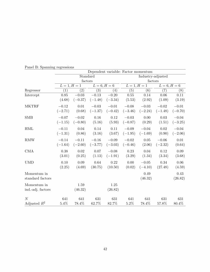
Panel B: Spanning regressionsDependent variable: Factor momentum

Standard Industry-adjustedfactors factors

L = 1, H = 1 L = 6, H = 6 L = 1, H = 1 L = 6, H = 6Regressor (1) (2) (3) (4) (5) (6) (7) (8)

Intercept 0.85 −0.03 −0.13 −0.20 0.55 0.14 0.06 0.11(4.68) (−0.37) (−1.48) (−3.34) (5.53) (2.92) (1.09) (3.19)

MKTRF −0.12 0.01 −0.03 −0.01 −0.08 −0.03 −0.02 −0.01(−2.71) (0.68) (−1.37) (−0.42) (−3.46) (−2.24) (−1.48) (−0.70)

SMB −0.07 −0.02 0.16 0.12 −0.03 0.00 0.03 −0.04(−1.15) (−0.80) (5.16) (5.93) (−0.87) (0.29) (1.51) (−3.25)

HML −0.11 0.04 0.14 0.11 −0.09 −0.04 0.02 −0.04(−1.31) (0.86) (3.16) (3.67) (−1.95) (−1.69) (0.90) (−2.06)

RMW −0.14 −0.11 −0.16 −0.09 −0.02 0.05 −0.06 0.01(−1.64) (−2.60) (−3.77) (−3.03) (−0.46) (2.06) (−2.32) (0.64)

CMA 0.38 0.02 0.07 −0.08 0.23 0.04 0.12 0.09(3.01) (0.25) (1.13) (−1.91) (3.29) (1.34) (3.34) (3.68)

UMD 0.10 0.09 0.64 0.22 0.00 −0.05 0.34 0.06(2.25) (4.69) (30.75) (10.50) (0.02) (−4.10) (27.48) (4.59)

Momentum in 0.49 0.43standard factors (46.32) (26.82)

Momentum in 1.59 1.25ind.-adj. factors (46.32) (26.82)

N 641 641 631 631 641 641 631 631Adjusted R2 5.4% 78.4% 62.7% 82.7% 5.2% 78.4% 57.8% 80.4%

42

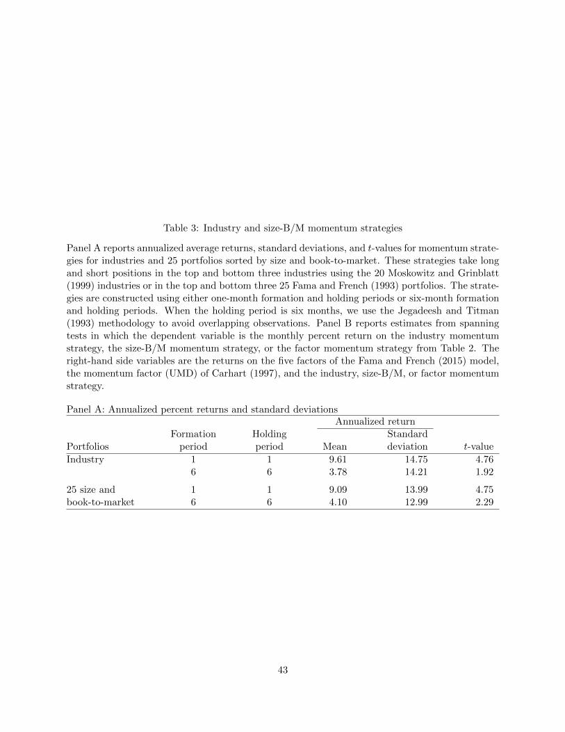
Table 3: Industry and size-B/M momentum strategies

Panel A reports annualized average returns, standard deviations, and t-values for momentum strate-gies for industries and 25 portfolios sorted by size and book-to-market. These strategies take longand short positions in the top and bottom three industries using the 20 Moskowitz and Grinblatt(1999) industries or in the top and bottom three 25 Fama and French (1993) portfolios. The strate-gies are constructed using either one-month formation and holding periods or six-month formationand holding periods. When the holding period is six months, we use the Jegadeesh and Titman(1993) methodology to avoid overlapping observations. Panel B reports estimates from spanningtests in which the dependent variable is the monthly percent return on the industry momentumstrategy, the size-B/M momentum strategy, or the factor momentum strategy from Table 2. Theright-hand side variables are the returns on the five factors of the Fama and French (2015) model,the momentum factor (UMD) of Carhart (1997), and the industry, size-B/M, or factor momentumstrategy.

Panel A: Annualized percent returns and standard deviationsAnnualized return

Formation Holding StandardPortfolios period period Mean deviation t-value

Industry 1 1 9.61 14.75 4.766 6 3.78 14.21 1.92

25 size and 1 1 9.09 13.99 4.75book-to-market 6 6 4.10 12.99 2.29

43

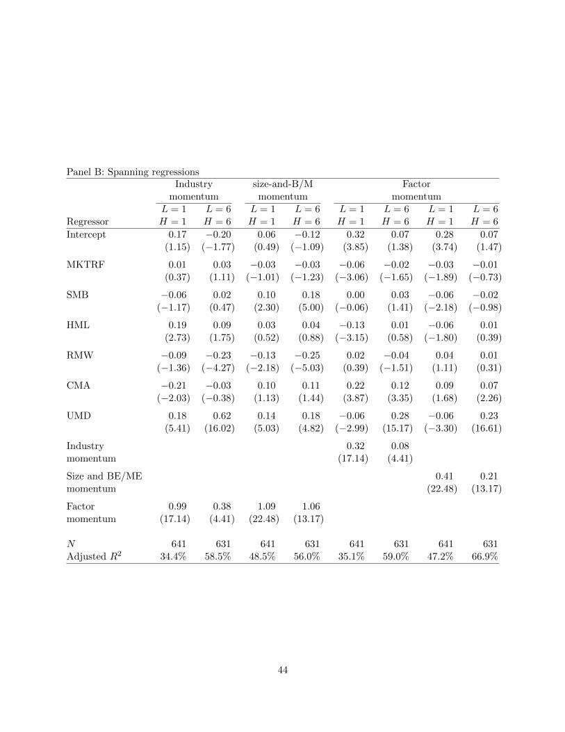
Panel B: Spanning regressionsIndustry size-and-B/M Factor

momentum momentum momentumL = 1 L = 6 L = 1 L = 6 L = 1 L = 6 L = 1 L = 6

Regressor H = 1 H = 6 H = 1 H = 6 H = 1 H = 6 H = 1 H = 6

Intercept 0.17 −0.20 0.06 −0.12 0.32 0.07 0.28 0.07(1.15) (−1.77) (0.49) (−1.09) (3.85) (1.38) (3.74) (1.47)

MKTRF 0.01 0.03 −0.03 −0.03 −0.06 −0.02 −0.03 −0.01(0.37) (1.11) (−1.01) (−1.23) (−3.06) (−1.65) (−1.89) (−0.73)

SMB −0.06 0.02 0.10 0.18 0.00 0.03 −0.06 −0.02(−1.17) (0.47) (2.30) (5.00) (−0.06) (1.41) (−2.18) (−0.98)

HML 0.19 0.09 0.03 0.04 −0.13 0.01 −0.06 0.01(2.73) (1.75) (0.52) (0.88) (−3.15) (0.58) (−1.80) (0.39)

RMW −0.09 −0.23 −0.13 −0.25 0.02 −0.04 0.04 0.01(−1.36) (−4.27) (−2.18) (−5.03) (0.39) (−1.51) (1.11) (0.31)

CMA −0.21 −0.03 0.10 0.11 0.22 0.12 0.09 0.07(−2.03) (−0.38) (1.13) (1.44) (3.87) (3.35) (1.68) (2.26)

UMD 0.18 0.62 0.14 0.18 −0.06 0.28 −0.06 0.23(5.41) (16.02) (5.03) (4.82) (−2.99) (15.17) (−3.30) (16.61)

Industry 0.32 0.08momentum (17.14) (4.41)

Size and BE/ME 0.41 0.21momentum (22.48) (13.17)

Factor 0.99 0.38 1.09 1.06momentum (17.14) (4.41) (22.48) (13.17)

N 641 631 641 631 641 631 641 631Adjusted R2 34.4% 58.5% 48.5% 56.0% 35.1% 59.0% 47.2% 66.9%

44

Table 4: Factor momentum strategies: Alternative sets of factors

This table reports average returns, alphas, and factors loadings of factor momentum strategies thatuse alternative sets of factors. “All” includes all 51 factors listed in Table 1; “Accounting-based”includes the 38 factors that use either income- or balance-sheet information, and that are rebalancedannually; “Return-based” includes the 13 factors that use return, volume, or price information, andthat are rebalanced monthly; and the “Fama-French five-factor model” includes the five factors ofthe Fama and French (2015) model. The last of these sets includes the market factor, and thefactors are those provided by Ken French at http://mba.tuck.dartmouth.edu/pages/faculty/

ken.french/data_library.html; the others specifications do not include the market factor andthe factors are the industry-adjusted versions listed in Table 1. Each factor momentum strategytakes long and short positions in the top and bottom max

{round( 3

20 ×N), 1}

factors, where N isthe number of factors in the set. The strategies use alternatively one- or six-month formation andholding periods. When the holding period is six months, we use the Jegadeesh and Titman (1993)methodology to avoid overlapping observations.

Accounting- Return- Fama-FrenchRegressor All based based five-factor model

Average monthly returns

r̄e 0.53 0.38 0.69 0.67(5.55) (5.71) (4.38) (3.30)

Monthly five-factor model + UMD alphas

Intercept 0.55 0.37 0.66 0.89(5.53) (5.31) (4.11) (4.37)

MKTRF −0.08 −0.06 −0.09 −0.36(−3.46) (−3.82) (−2.24) (−7.17)

SMB −0.03 0.03 −0.18 −0.03(−0.87) (1.07) (−3.19) (−0.48)

HML −0.09 −0.04 −0.17 −0.07(−1.95) (−1.06) (−2.16) (−0.72)

RMW −0.02 −0.04 0.12 −0.29(−0.46) (−1.26) (1.60) (−3.04)

CMA 0.23 0.14 0.44 0.19(3.29) (2.96) (3.94) (1.31)

UMD 0.00 0.03 0.01 0.01(0.02) (1.99) (0.39) (0.17)

N 641 641 641 641Adjusted R2 5.2% 6.3% 8.4% 10.3%

45

Table 5: Factor momentum strategies: A sensitivity analysis

Panel A lists the 51 factors sorted by momentum score. We compute each factor’s momentum scoreusing a three-step bootstrapping procedure. First, we draw a random set of ten factors, constructa factor momentum strategy with one-month formation and holding periods, and compute thisstrategy’s average return. Second, we drop each factor at a time, construct a factor momentumstrategy from the remaining nine factors, and compute the reduction in the strategy’s average returnrelative to that of the original strategy with ten factors. Third, we repeat these computations for10,000 random sets of ten factors each. A factor’s momentum score is the bootstrapped t-valueassociated with the average reduction in the average return that results from dropping each factor.We multiply these t-values by −1; a high value indicates that the factor contributes more towardsfactor momentum profits. Panel B reports average monthly returns and five-factor model plusUMD alphas for five factor momentum strategies. In the in-sample analysis we assign the 51factors into quintiles based on Panel A’s momentum scores and construct the momentum strategywithin each quintile. Each strategy is long the top two factors and short the bottom two factors.In the out-of-sample analysis we first compute momentum scores using data on even months andthen measure the out-of-sample (that is, odd-month) performance of the five strategies formed bythe momentum scores. We then repeat this computation by computing the scores using odd-monthdata and measure the strategies’ even-month performance. We merge the out-of-sample even- andodd-month returns.

46

Panel A: Momentum scoresFactor Factorrank Factor t-value rank Factor Score1 Firm age 4.57 27 Investment to assets 0.752 Short-term reversals 3.60 28 Profit margin 0.703 Nominal price 3.51 29 Enterprise multiple 0.684 Intermediate momentum 3.03 30 Earnings to price 0.645 Idiosyncratic volatility 2.69 31 Debt issuance 0.476 Leverage 2.27 32 Abnormal investment 0.457 Sales to price 2.02 33 Growth in inventory 0.428 Book-to-market 1.95 34 Gross profitability 0.399 Distress risk 1.76 35 Operating profitability 0.3810 Altman’s Z-score 1.64 36 Cash-based profitability 0.3311 Return on assets 1.49 37 Investment growth rate 0.2912 Asset growth 1.40 38 Total external financing 0.2813 Momentum 1.33 39 Net operating assets 0.1214 Maximum daily return 1.22 40 M/B and accruals 0.0915 QMJ Profitability 1.18 41 Piotroski’s F-score 0.0216 Ohlson’s O-score 1.18 42 Five-year share issuance −0.0217 Investment-to-capital 1.06 43 Sustainable growth −0.0418 Market beta 1.04 44 Sales growth −0.1119 Amihud’s illiquidity 1.03 45 Net working capital changes −0.2520 Cashflow to price 1.02 46 Accruals −0.6321 Long-term reversals 0.95 47 Change in asset turnover −0.6922 Size 0.95 48 Industry-adjusted CAPX growth −0.8723 Heston-Sadka seasonality 0.91 49 One-year share issuance −0.8724 52-week high 0.88 50 Sales-inventory growth −0.9125 Return on equity 0.81 51 High-volume return premium −1.3526 Industry concentration 0.79

47

Panel B: Factor momentum strategies formed from factors sorted by momentum scoreMomentum Full sample Out-of-samplescore Average FF5+UMD Average FF5+UMDquintile return alpha return alpha

1 0.09 0.10 0.22 0.22(2.24) (2.28) (4.72) (4.63)

2 0.24 0.22 0.35 0.44(4.25) (3.77) (4.13) (4.94)

3 0.37 0.49 0.43 0.42(3.68) (4.70) (5.25) (4.91)

4 0.49 0.47 0.39 0.39(4.37) (4.00) (4.15) (3.94)

5 0.87 0.83 0.66 0.64(6.76) (6.29) (4.55) (4.29)

5 − 1 0.77 0.73 0.44 0.41(6.92) (6.38) (3.44) (3.14)

48

Table 6: Robustness: Implementation delay and small versus big factors

This table reports average returns and five-factor model plus UMD alphas for factor momentumstrategies. Each strategy uses one-month formation and holding periods to trade the 51 factorslisted in Table 1. In columns “Number of trading days skipped” we begin measuring returns atthe close of month t (trading days skipped = 0), one trading day later, two trading days later, orthree trading days later. In columns “Factor size” we construct the factors separately from smalland big stocks. The standard HML factor, for example, is defined in Fama and French (1993) as

HMLt =1

2

(rsmall valuet + rbig value

t

)− 1

2

(rsmall growth

t + rbig growth

t

).

We follow Fama and French (2016a) and define small and big HML factors as

HMLsmallt = rsmall value

t − rsmall growth

t ,

HMLbig

t = rbig value

t − rbig growth

t .

We construct the factor momentum strategies separately from small and big factors. We drop sizefactor from the analysis when constructing factor momentum strategies from the small and bigfactors.

49

Number of trading days skipped Factor sizeRegressor 0 1 2 3 Small Big

Average monthly returns

r̄e 0.53 0.49 0.43 0.37 0.63 0.33(5.53) (5.10) (4.67) (4.16) (5.39) (4.08)

Monthly five-factor model + UMD alphas

Intercept 0.55 0.49 0.41 0.34 0.61 0.32(5.52) (4.87) (4.38) (3.72) (5.02) (3.81)

MKTRF −0.08 −0.09 −0.09 −0.09 −0.06 −0.09(−3.43) (−3.68) (−4.10) (−4.23) (−2.12) (−4.56)

SMB −0.03 0.00 0.02 0.04 −0.05 0.01(−0.89) (0.09) (0.59) (1.24) (−1.09) (0.38)

HML −0.09 −0.09 −0.09 −0.08 −0.13 −0.02(−1.94) (−1.84) (−1.89) (−1.76) (−2.16) (−0.42)

RMW −2.24 −0.53 −0.51 1.16 0.01 0.04(−0.47) (−0.11) (−0.11) (0.27) (0.12) (1.10)

CMA 22.85 22.82 21.39 20.92 0.35 0.15(3.28) (3.28) (3.24) (3.33) (4.18) (2.60)

UMD 0.00 0.02 0.04 0.04 0.00 0.01(0.00) (0.87) (1.69) (2.12) (−0.11) (0.56)

N 641 641 641 641 641 641Adjusted R2 5.2% 5.5% 6.6% 7.3% 5.0% 7.4%

50

Table 7: Short-term reversals and individual stock, industry, and factor momentum

This table reports estimates from spanning regressions in which the dependent variable is themonthly return on the short-term reversals factor (Panel A) or the individual stock momentumfactor (Panel B), and the independent variables are the market, size, value, profitability, andinvestment factors of the Fama and French (2015) five-factor model, the stock momentum factor ofCarhart (1997), and the monthly returns on the industry and factor momentum strategies. Boththe industry and factor momentum strategies use one-month formation and holding periods. Theindustry momentum strategy ranks the 20 Moskowitz and Grinblatt (1999) industries based ontheir past returns and takes long and short positions in the top and bottom three industries. Thefactor momentum strategy ranks the 51 factors listed in Table 1 and takes long and short positionsin the top and bottom eight factors.

Panel A: Dependent variable: Short-term reversals (STREV)Regression

Regressor (1) (2) (3) (4) (5)

Intercept 0.37 0.51 0.85 1.00 1.05(3.05) (4.19) (9.49) (12.05) (14.39)

MKTRF 0.17 0.15 0.12 0.07 0.08(5.75) (5.09) (5.44) (3.73) (4.47)

SMB 0.09 0.11 0.07 0.08 0.06(2.17) (2.57) (2.15) (2.86) (2.62)

HML 0.20 0.10 0.15 0.02 0.07(3.44) (1.77) (3.52) (0.47) (2.04)

RMW −0.01 0.04 −0.02 0.02 −0.01(−0.12) (0.68) (−0.37) (0.51) (−0.17)

CMA −0.23 −0.15 −0.14 0.06 0.00(−2.61) (−1.78) (−2.30) (0.97) (−0.02)

UMD −0.18 −0.10 −0.18 −0.13(−6.48) (−4.61) (−9.63) (−7.83)

Industry −0.47 −0.27momentum (−23.73) (−13.92)

Factor −0.90 −0.63momentum (−27.77) (−18.38)

N 641 641 641 641 641Adjusted R2 9.6% 15.1% 55.0% 61.7% 70.6%

51

Panel B: Dependent variable: Individual stock momentum (UMD)Regression

Regressor (1) (2) (3) (4) (5)

Intercept 0.72 0.85 0.85 1.36 1.31(4.31) (5.19) (4.83) (8.08) (7.43)

MKTRF −0.13 −0.07 −0.07 −0.05 −0.05(−3.11) (−1.68) (−1.68) (−1.27) (−1.35)

SMB 0.08 0.11 0.11 0.13 0.13(1.29) (1.88) (1.88) (2.48) (2.47)

HML −0.53 −0.46 −0.46 −0.44 −0.44(−6.69) (−5.96) (−5.91) (−5.89) (−5.95)

RMW 0.25 0.25 0.25 0.25 0.25(3.15) (3.22) (3.22) (3.35) (3.38)

CMA 0.41 0.33 0.33 0.39 0.40(3.48) (2.90) (2.90) (3.59) (3.64)

STREV −0.34 −0.34 −0.77 −0.73(−6.48) (−4.61) (−10.54) (−8.62)

Industry 0.00 0.04momentum (0.05) (0.86)

Factor −0.80 −0.81momentum (−8.08) (−8.12)

N 641 641 641 641 641Adjusted R2 8.9% 14.4% 14.3% 22.3% 22.2%

52