factormodelforecastsofexchangerates - sscc - homecengel/publishedpapers/factorforecasts.pdf · that...

12345678910111213141516171819202122232425262728293031323334353637383940414243

Econometric Reviews, 0(0):1–24, 2014Copyright © Taylor & Francis Group, LLCISSN: 0747-4938 print/1532-4168 onlineDOI: 10.1080/07474938.2014.944467

FactorModel Forecasts of Exchange Rates

Charles Engel1, Nelson C. Mark2, and Kenneth D. West31University of Wisconsin, Wisconsin, USA

2University of Notre Dame3Department of Economics, University of Wisconsin, Madison, Wisconsin, USA

We construct factors from a cross-section of exchange rates and use the idiosyncraticdeviations from the factors to forecast. In a stylized data generating process, we showthat such forecasts can be effective even if there is essentially no serial correlation in theunivariate exchange rate processes. We apply the technique to a panel of bilateral U.S. dollarrates against 17 OECD countries. We forecast using factors, and using factors combinedwith any of fundamentals suggested by Taylor rule, monetary and purchasing power parity(PPP) models. For long horizon (8 and 12 quarter) forecasts, we tend to improve on theforecast of a “no change” benchmark in the late (1999–2007) but not early (1987–1998) partsof our sample.

Keywords �.

JEL Classification �.

1. INTRODUCTION

In predictions of floating exchange rates between countries with roughly similar inflation

Q1

Q2

rates, a random walk model works very well. The random walk forecast is one in whichthe (log) level of the nominal exchange rate is predicted to stay at the current log level;equivalently, the forecast is one of “no change” in the exchange rate. This forecast workswell at various horizons, from one day to three years. It does well in the followingsense: the out of sample mean squared (or mean absolute) error in predicting exchangerate movements generally is about the same, and often smaller, than that of modelsthat use “fundamentals” data on variables such as money, output, inflation, productivity,and interest rates. Classic references are Meese and Rogoff (1983a,b); a recent update isCheung et al. (2005).

Whether or not this stylized regularity is bad news for economic theory is unclear.Some economists think the regularity is very bad news. Bacchetta and van Wincoop

Address correspondence to Kenneth West, Department of Economics, University of Wisconsin, 1180Observatory Dr., Madison, WI 53706, USA; E-mail: [email protected]

Color versions of one or more of the figures in the article can be found online at www.tandfonline.com/lecr.

44454647484950515253545556575859606162636465666768697071727374757677787980818283848586

2 C. ENGEL ET AL.

(2006, p. 552) describe it as “� � � the major weakness of international macroeconomics.”On the other hand, Engel and West (2005) argue that a near random walk is expectedunder certain conditions.1

Whether or not one thinks the empirical finding of near random walk behavior is badnews for economic theory, it is of interest to try to tease out connections (if any) betweena given exchange rate and other data. A small literature has used panel data techniquesto forecast exchange rates, finding relatively good success (Mark and Sul, 2001; Rapachand Wohar, 2004; Groen, 2005; Engel et al., 2008). A very large literature has foundthat factor models do a good job forecasting basic macro variables.2 The present paperpredicts exchange rates, via factor models, in the context of panel data estimation, andcompares the predictions to those of a random walk via root mean squared predictionerror.

The panel consists of quarterly data on 17 bilateral U.S. dollar exchange rates withOECD countries, 1973–2007. We construct factors from the exchange rates. We take Q3the literature on predicting exchange rates to suggest that the exchange rate seriesthemselves have information that is hard to extract from observable fundamentals. Thisinformation might be hard to extract because standard measures of fundamentals (e.g.,money supplies and output) are error ridden, or because we simply lack any directmeasures of nonstandard fundamentals such as risk premia or noise trading.3

We compare four different forecasting models to a benchmark model that makes a“no-change” forecast—the random walk model. One of our four models uses factors butno other variables to forecast. The other three use factors along with some measures ofobservable fundamentals. The three measures of observable fundamentals are as follows:(1) those of a “Taylor rule” model; (2) those of a monetary model; and (3) deviations frompurchasing power parity (PPP). Our measure of forecasting performance is root meansquared prediction error (root MSPE).

On balance, these models have lower MSPE than does a random walk model forlong (8 and 12 quarter) horizon predictions over the late part of our forecasting sample(1999–2007). These differences, however, are usually not significant at conventional levels.Predictions that span the entire two decades (1987–2007) or the early part (1987–1998)of our forecast sample generally have higher MSPE than does a no-change forecast.(Different samples involve different currencies, because of the introduction of the Euro in1999.) The basic factor model and the factor model supplemented by PPP fundamentals

1The Engel and West (2005) argument is not that a random walk is produced by an efficient market;indeed the simple efficient markets model implies that exchange rate changes are predicted by interest ratedifferentials and any variables correlated with interest rate differentials. Rather, the argument relates to thebehavior of an asset price that is determined by a present value model with a discount factor near 1.

2See Stock and Watson (2006). We use “factor” to refer to a data generating process driven by factors,even if the estimation technique involves principal components.

3See Diebold et al. (1994) for another attempt, with methodology very different from ours, to predictexchange rates using a cross section of exchange rates.

87888990919293949596979899100101102103104105106107108109110111112113114115116117118119120121122123124125126127128129

FACTOR MODEL FORECASTS OF EXCHANGE RATES 3

do best. We recognize that the good performance in the recent period may be ephemeral.But we are hopeful that our approach will prove useful in other datasets.

We close this introduction with some cautions. First, we make no attempt to justifyor defend the use of out of sample analysis. We and others have found such analysisuseful and informative. But we recognize that some economists might disagree. Second,judgment (sometimes rather arbitrary) has been used at various stages, so we are not(yet) proposing a completely replicable strategy. Third, our exercise is not “true” out ofsample. For example, revised rather than real time data are used in some specifications.We use revised data because we are using out of sample analysis as a model evaluationtool, and the models presume that the best available data are used. More importantly,perhaps, our exercise is not true out of sample because we have relied on research thathas already examined exchange rates during parts of our forecasting sample. The mostpertinent reference is Engel et al. (2008), which used similar data, spanning 1973–2005 (vs.1973–2007). Finally, we limit ourselves to simple linear models; papers such as Bulut andMaasoumi (2012) suggest that such models miss essential features of exchange rate data.

Section 2 presents a stylized model that illustrates analytically why our approach mightpredict well. Section 3 describes our empirical models. Section 4 our data and forecastevaluation techniques. Section 5 presents empirical results, Section 6 robustness checks,and Section 7 concludes. An appendix includes some algebraic details. Some additionalappendices, available on request, present detailed empirical results omitted from the paperto save space.

2. WHY A FACTOR MODEL MAY FORECAST WELL

In this section, we present a factor model and a simple data generating process thatmotivates its use.

Our basic presumption is that the deviation of the exchange rate from a measureof central tendency will help predict subsequent movements in the exchange rate.Algebraically, let

sit = log of exchange rate in country i in period t, (2.1)

zit = measure of central tendency defined below�

For concreteness, we note that sit is measured as log(foreign currency units/U.S. dollar),though that is not relevant to the present discussion. Algebraically, our basic presumptionis that for a horizon h, sit+h − sit can be predicted by zit − sit, maybe using two differentmeasures of z in a single regression.

Many papers have relied on the same presumption (that sit+h − sit can be predicted byzit − sit). For example, Mark (1995) sets zit in accordance with the “monetary model,”so that zit depends on money supplies and output levels; Molodtsova and Papell (2008)set zit in accordance with a “Taylor rule” model, so that zit depends on the exchange

130131132133134135136137138139140141142143144145146147148149150151152153154155156157158159160161162163164165166167168169170171172

4 C. ENGEL ET AL.

rate, inflation rates, output gaps, and parameters of monetary policy rules; Engel et al.(2008) set zit in accordance with PPP, so that zit depends on price levels. Some papers (seereferences above) have used these specifications of zit in the context of panel data. Ourtwist is to construct one measure of zit from factors estimated from the panel of exchangerates.

To exposit the idea, consider the following example. Suppose that the ith exchange ratefollows the process

sit = Fit + vit� (2.2)

Here, Fit is the effect the factor has on currency i; in a one factor model, for example Fit =�if1t where f1t is the factor and �i is the factor loading for currency i. The idiosyncraticshock vit is uncorrelated with Fit. For simplicity, make as well some further assumptionsnot required in our empirical work, namely, that Fit follows a random walk and that vitis i.i.d.: Q4

Fit = Fit−1 + �it, �it ∼ i.i.d. (0, �2�), vit ∼ i.i.d. (0, �2

v), E�itvis = 0 all t, s� (2.3)

An i subscript is omitted from the variances �2� and �2

v for notational simplicity.Then �sit = �it + vit − vit−1 and the univariate process followed by �sit is clearly an

MA(1), say

�sit = �it + ��it−1, E�2it ≡ �2�, |�| < 1� (2.4)

Here, �it is the Wold innovation in �sit. The variance of �it and the value of � can becomputed in straightforward fashion from the values of �2

� and �2v .4

Let us compare population forecasts of �sit+1 using the factor model (2.2), the MA(1)model (2.4), and a random walk model. As above, let “MSPE” denote “mean squaredprediction error.” Unless otherwise stated, in this section MSPE refers to a populationrather than sample quantity. (This contrasts to the discussion of our empirical workbelow, in which MSPE refers to a sample quantity.) To forecast using (2.2), observe that�sit+1 = �Fit+1 + �vit+1 = �it+1 + vit+1 − vit ⇒ Et�sit+1 = −vit ≡ Fit − sit ⇒

forecast error from factor model = �it+1 + vit+1, MSPEfactor = �2� + �2

v � (2.5)

The MSPE from the univariate model (2.4) is of course �2�. With a little bit of algebra, and

using the formula for �2� given in the previous footnote, it may be shown that �2

� + �2v <

�2�. Hence the factor model has a lower MSPE than the MA(1) model.But the relevant issue is whether the improvement (i.e., the fall) in the MSPE is notable,

for a plausible data generating process. A plausible data generating process (DGP) would

4Specifically, let � = �2� + 2�2

v denote the variance of �s. Then �2� = 0�5[� + (�2 − 4�4

�)1/2], � = −�2

v/�2� .

173174175176177178179180181182183184185186187188189190191192193194195196197198199200201202203204205206207208209210211212213214215


be one in which there is very little serial correlation in �sit. Put differently, if the DGP issuch that the MSPE from the MA(1) model is essentially the same as that from a randomwalk model, is it still possible that the MSPE from the factor model is substantiallysmaller than that of the random walk?

In our empirical work, we use Theil’s U-statistic to compare (sample) MSPEs relativeto that of a random walk. These are square roots of the following ratio: sample MSPEalternative forecast/sample MSPE forecast of no change. The forecast error of therandom walk model is the actual change in �sit = �it + vit − vit−1; the correspondingpopulation MSPE is �2

� + 2�2v . In the context of the present section (population rather

than MSPEs), define population U-statistics as

Ufactor = [(�2� + �2

v)/(�2� + 2�2

v)]1/2, UMA = [�2�/(�

2� + 2�2

v)]/2� (2.6)

For select values of the first order autocorrelation of �sit (which is approximately the MAparameter � introduced in (2.4)), these are as follows:

corr(�sit,�sit−1) −0�01 −0�02 −0�03 −0�04 −0�05 −0�10, (2.7a)UMA 0�99995 0�9998 0�9996 0�9992 0�9987 0�9949, (2.7b)Ufactor 0�995 0�990 0�985 0�980 0�975 0�949� (2.7c)

The factor model improves on the moving average model by an order of magnitude. Forexample, when the first order autocorrelation of �sit is −0.10, the population root MSPEfor the MA model is only 0.5% lower than for the random walk (because 0.9949 is about0.5% smaller than 1), while the population root MSPE for the factor model is about 5%lower than the random walk.

We further note that the population values for UMA in (2.7b) are so near 1 that inpractice, for any of the values of the autocorrelations, one would not be surprised ifsampling error in estimation of an MA(1) model led to sample U-statistics above 1.Hence, we view the figures in the table as consistent with the well-established finding thatno univariate model predicts better than a random walk. But clearly the factor model hasthe potential to predict better, even accepting the point that in practice the best univariatemodel is a random walk.

In the simple DGP consisting of (2.2) and (2.3), whether a factor model will havelower MSPE than a model that uses information not only on exchange rates but alsoon fundamentals such as prices and output depends on whether the additional variableshelp pin down vit. To allow for this possibility, our empirical work combines factors withobservable fundamentals, as discussed in the next section.

3. EMPIRICAL MODELS

We use models with one, two or three factors. We will use the three factor model forillustration. The one and two factor models are analogous. In the three factor model,

216217218219220221222223224225226227228229230231232233234235236237238239240241242243244245246247248249250251252253254255256257258

6 C. ENGEL ET AL.

we first estimate a set of three factors and factor loadings from the exchange rates. Forcurrency i, i = 1, � � � , 17, the model is

sit = constant + �1if1t + �2if2t + �3if3t + vit

≡ constant + Fit + vit� (3.1)

The factors (the f ’s) are unobserved I(1) variables. Here and throughout, we do notattempt to test for unit roots in the factors or any other variable for that matter. See Bai(2004) on estimation of factor models with unit root data.

Let Fit = �1if1t + �2if2t + �3if3t. We aim to use (estimates of) Fit to forecast sit. Incontrast to much work with factors, the factors are not constructed from a set ofadditional variables. For example, in Groen’s (2006) work on exchange rates, factorsare constructed from data on real activity and prices, and take the place of traditionalmeasures of real and nominal activity. We take the literature on predicting exchange ratesto suggest that the exchange rate series themselves may have low frequency informationon common trends that is hard to extract from observable fundamentals. This lowfrequency information might be buried in standard, but noisy, measures of fundamentalssuch as relative money supplies and relative outputs. Or this information might beembedded in nonstandard measures of fundamentals that are sufficiently persistent thatthey function in part to drive common trends; examples are persistent risk premiaor persistent noise trading. Put differently, we use factors to parsimoniously captureco-movements of exchange rates that are not well-captured by observable fundamentals.Crudely, we posit that a weighted average of the log levels of exchange rates represents acentral tendency for the log level a given exchange rate, and use this weighted average tohelp forecast.

Mechanics are as follows. We assume that the factors component soaks up a commonunit root component in the s’s. That is, we assume that Fit − sit is stationary and maybe useful in predicting (stationary) future changes in sit. We do not attempt to teststationarity of vit; our selection of number of factors was based on presumed limitationsof a panel of cross-section dimension 17.5 The factors f1t, f2t, and f3t are uncorrelated byconstruction. We normalize the f ’s to have mean zero and unit variance.

So this first stage produces a time series for f1t, f2t, and f3t and factor loadings, �1i,i = 1, � � � , 17; �2i, i = 1, � � � , 17; �3i, i = 1, � � � , 17. In our simplest specification, the measureof central tendency zit that was introduced in (2.1) is

zit = �1if1t + �2if2t + �3if3t ≡ Fit� (3.3)

5In principle, one could use techniques to determine cointegrating rank to determine the number of I(1)factors and the factor loadings. We take results such as Ho and Sørensen (1996) to indicate that the finitesample performance of such techniques is likely to be poor, when the cross-section dimension is 17.

259260261262263264265266267268269270271272273274275276277278279280281282283284285286287288289290291292293294295296297298299300301


In this simplest specification, with Fit ≡ �1if1t + �2if2t + �3if3t, for quarterly horizonsh = 1, 4, 8, and 12 we use a standard panel data estimator (least squares with dummyvariable) to estimate and forecast. For example, with a horizon of h = 4 quarters, weestimate

sit+4 − sit = i + (Fit − sit) + uit+4, (3.4)

where i is a fixed effect for country i. We then use i and to predict (some detailsbelow). Here, and in all of our specifications, there is no “time effect” (in the jargon ofpanel data): the factors are dynamic versions of time effects (we hope).

Our three other specifications combine factors with observables. The other threespecifications are all of the form

sit+h − sit = i + (Fit − sit) + �(zit − sit) + uit+h, (3.5)

for three different zit’s. Let country 0 refer to the USA. The three zit’s are as follows:

Taylor rule: zit = 1�5(�it − �0t) + 0�5(yit − y0t) + sit; � = inflation, y = output gap;

zit − sit = 1�5(�it − �0t) + 0�5(yit − y0t); (3.6)

monetary model: zit = (mit − m0t) − (yit − y0t); m = ln(money), y = ln(output);(3.7)

PPP model: zit = pit − p0t; p = ln(price level)� (3.8)

The Taylor rule model builds on the recently developed view that interest rates ratherthan money supplies are the instrument of monetary policy. Expositions may be foundin Benigno and Benigno (2006), Engel and West (2006), and Mark (2008). The monetarymodel was for many years the workhorse of international monetary economics; see, forexample the textbook exposition in Mark (2001) or the abbreviated summary in Engeland West (2005). The PPP model (3.6) presumes convergence of price levels.

4. DATA AND FORECASTING EVALUATION

We use quarterly data, 1973:1–2007:4, with the out of sample period beginning in 1987:1.The basic data source is International Financial Statistics, supplemented on occasionby national sources. Exchange rates are end of quarter values of the U.S. dollar vs.the currencies of 17 OECD countries: Australia, Austria, Belgium, Canada, Denmark,Finland, France, Germany, Japan, Italy, Korea, Netherlands, Norway, Spain, Sweden,Switzerland, and the United Kingdom. (See below on how we handled conversion tothe Euro in 1999:1.) The price level is the CPI in the last month of the quarter; Q5output is industrial production in last month of the quarter; money is M1 (with

302303304305306307308309310311312313314315316317318319320321322323324325326327328329330331332333334335336337338339340341342343344

8 C. ENGEL ET AL.

some complications); the output gap is constructed by HP detrending, computedrecursively, using only data from periods prior to the forecast period. Because someof the data appeared to display seasonality, we seasonally adjusted prices, output andmoney by taking a four quarter average of the log levels before doing any empiricalwork. For example, the price level in country i is pit = 1/4[log(CPIit) + log(CPIit−1) +log(CPIit−2) + log(CPIit−3)].

To explain the mechanics of our forecasting work, let us illustrate for the four quarterhorizon (h = 4), for the first forecast, and for the model that uses only factors but notadditional observable fundamentals. As depicted in (4.1) below, we use data from 1973:1to 1986:4 to estimate factors and factor loadings, and construct Fit for i = 1, � � � , 17.

We then use right hand side data from 1973:1 to 1985:4 to estimate panel data regression

sit+4 − st = i + (Fit − sit) + uit+4, t = 1973 : 1, � � � , 1985 : 4� (4.2)

We use 1986:4 data to predict the 4 quarter change in s:

Prediction of (si,1987:4 − si,1986:4) = i + (Fi,1986:4 − si,1986:4)� (4.3)

We then add an observation to the end of the sample, and repeat.As is indicated by this discussion, the recursive method is used to generate predictions:

observations are added to the end of the estimation sample, so that the sample size usedto estimate factors and panel data regressions grows. The direct (as opposed to iterated)method is used to make multiperiod predictions. The estimation technique is maximumlikelihood, assuming normality.

An analogous setup is used for other horizons and for models with observablefundamentals.

For a given date, factors and r.h.s. variables are identical across horizons: for givent, the same values of Fit − sit are used. However, the l.h.s. variable is different (h perioddifference in st), and regression samples are smaller for larger h. This means that theregression coefficients (i, ) and predictions vary with h.

For the 9 non-Euro currencies (Australia, Canada, Denmark, Japan, Korea, Norway,Sweden, Switzerland, and the United Kingdom), we report “long sample” forecastingstatistics for a 1987–2007 sample. For all 17 currencies, we report “early” sampleforecasting statistics for a 1987–1998 sample. For the 9 non-Euro currencies and theEuro, we report “late sample” forecasting statistics for a 1999–2007 sample. Early samplestatistics involve forecasts whose forecast base begins in 1986:4 and ends in 1998:4.Towards the end of the early sample, the forecast occurs in the pre-Euro era, while the

345346347348349350351352353354355356357358359360361362363364365366367368369370371372373374375376377378379380381382383384385386387


TABLE 1List of Currencies and Models

A. Number of Quarterly Observations in Prediction Sample

Prediction sample Horizon h

1 4 8 12Long Sample (1986 : 4 + h) − 2007 : 4 84 81 77 73Early Sample (1986 : 4 + h) − (1998 : 4 + h) 49 49 49 49Late Sample (1999 : 1 + h) − 2007 : 4 35 32 28 24

B. Currencies

Long sample N = 9 Australia, Canada, Denmark, Japan, Korea, Norway, Sweden, Switzerland, UnitedKingdom

Early sample N = 17 The long sample countries plus: Austria, Belgium, Finland, France, Germany,Italy, Netherlands and Spain

Late Sample N = 10 The long sample countries plus the Euro

C. Models

Fit − sit Fit is the estimated factor component of currency i, estimated from 17 currenciesin each sample (with identical Euro values appearing post-1998 for the 8 Euroarea currencies).

Fit − sit + Taylor Taylor rule fundamentals (3.6) also included as a regressorFit − sit + Monetary Monetary model fundamentals (3.7) also included as a regressorFit − sit + PPP Purchasing power parity fundamentals (3.8) also included as a regressor

Notes: 1. The sample period for estimation of models runs from 1973:1 to the forecast base. Models areestimated recursively. Factors are estimated using N = 17 currencies, for all samples. 2. In the late sample,Euro area forecasts are made by averaging forecasts from the 8 Euro countries. 3. Long horizon forecastsare made using the direct method.

realization occurs during the Euro era. We rescaled Euro area currencies so that therewas no discontinuity. See Table 1 for the exact number of forecasts for each sample andhorizon, as well as a summary listing of models.

In all samples (long, early and late), we use data from all 17 countries to constructfactors and panel data estimates. For post-1999 data, the left hand side variable in bothfactor and panel data estimation is identical for all 8 Euro area countries. But because allsamples include some pre-1999 data in estimation, there are differences across countriesin estimates of the factor Fit, and of course the measures of prices, output and moneyused in the PPP, monetary and Taylor rule models. This means that the forecasts aredifferent for the Euro countries. We construct a Euro forecast by simple averaging of the8 different forecasts.

Our measure of forecast performance is root mean squared prediction error (RMSPE).(Here and through the rest of the paper, all references to MSPE and RMSPE referto sample rather than population values.) We compute Theil’s U-statistic, the ratio ofthe RMSPE from each of our models to the RMSPE from a random walk model.

388389390391392393394395396397398399400401402403404405406407408409410411412413414415416417418419420421422423424425426427428429430

10 C. ENGEL ET AL.

We summarize results by reporting the median (across 17 countries) of the U-statistic,and the number of currencies for which the ratio is less than one (since a value less thanone means our model had smaller RMSPE than did a random walk). Individual currencyresults are available on request.

A U-statistic of 1 indicates that the (sample) RMSPEs from the factor model and fromthe random walk are the same. As argued by Clark and West (2006, 2007), this is evidenceagainst the random walk model. If, indeed, a random walk generates the data, then thefactor model introduces spurious variables into the forecasting process. In finite samples,attempts to use such variables will, on average, introduce noise that inflates the variabilityof the forecasting error of the factor model. Hence, under a random walk null, we expectsample U-statistics greater than 1, even though that null implies that population ratios ofRMSPEs are 1.

We report 10% level one sided hypothesis tests on H0: RMSPE(our model) =RMSPE(random walk) against HA: RMSPE(our model) < RMSPE(random walk). (Here,“our model” refers to any one of the four models given in (3.4) or (3.6)–(3.8): factor model,factor model plus Taylor rule, factor model plus monetary, or factor model plus PPP.)These hypothesis tests are conducted in accordance with Clark and West (2006), whodevelop a test procedure that accounts for the potential inflation of the factor model’sRMSPE noted in the previous paragraph. Of course, with many currencies (17, in ourearly sample), it is very possible that one or more test statistics will be significant evenif none in fact predict better than a random walk. We guarded against this possibilityby testing H0: RMSPE(our model) = RMSPE(random walk) for all currencies againstHA: RMSPE(our model) > RMSPE(random walk) for at least one currency, using theprocedure in Hubrich and West (2010).6 This statistic, however, rarely had a p-valueless than 0.10. We therefore do not report it, to keep down the number of figuresreported.

5. EMPIRICAL RESULTS

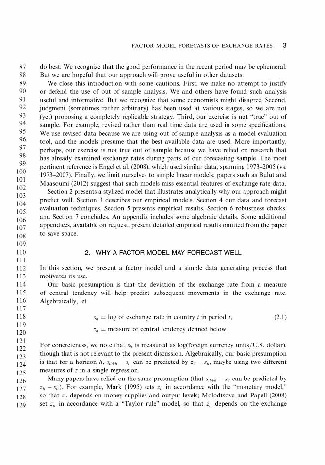
For the largest sample used (1973–2007), Fig. 1 plots the estimates of the three factors,while Table 2 presents the factor loadings. The factor loadings in Table 2 are organizedso that the first block of six currencies (Austria, ... ,Switzerland) includes currencies in theone-time German mark area. The next block of four currencies (Finland, ... ,Spain) are

6Although we report ratios of MSPEs, the Clark and West (2006) and Hubrich and West (2008) tests workoff arithmetic difference of MSPEs, evaluating whether this difference is statistically different from zero. The nullhypothesis is that the random walk generates the data. These tests begin by adjusting the MSPE difference toaccount for noise that is present in the alternative (the nonrandom walk model) under the null hypothesis. ForClark and West (2006), the standard Diebold–Mariano–West (DMW) statistic is then computed for the adjustedMSPE difference. For Hubrich and West (2009), a parametric bootstrap is executed, under the assumptionof normality. We did 10,000 repetitions in this bootstrap. See West (1996, 2006) for basic theory and furtherdiscussion.

431432433434435436437438439440441442443444445446447448449450451452453454455456457458459460461462463464465466467468469470471472473


FIGURE 1 Factors, 1973–2007 sample.

Euro area countries not included in the first block. The final block (Australia,...,UK) liststhe seven remaining countries.

The factor loadings suggest that the second factor reflects a central tendency ofcountries in the former German mark area. (If the factor loading on the second factorwas zero for countries not in the mark area, then this second factor would literally bea weighted average of countries in the mark area (see Stock and Watson, 2006). The

474475476477478479480481482483484485486487488489490491492493494495496497498499500501502503504505506507508509510511512513514515516

12 C. ENGEL ET AL.

TABLE 2Factor Loadings, 1973–2007 Sample

�1i �2i �3i

Austria −0�06 1�00 0�02Belgium 0�53 0�83 −0�11Denmark 0�70 0�68 −0�16Germany −0�03 1�00 0�01Netherlands 0�08 1�00 −0�02Switzerland −0�31 0�93 −0�03Finland 0�88 0�23 0�34France 0�85 0�50 −0�16Italy 0�97 −0�14 0�15Spain 0�98 −0�08 0�12Australia 0�87 −0�31 0�16Canada 0�80 −0�11 0�29Japan −0�55 0�78 −0�16Korea 0�84 −0�27 0�28Norway 0�95 0�19 0�12Sweden 0�96 −0�07 0�22UK 0�84 0�13 −0�01

Notes: 1. The fitted model is sit = const. + �1if1t + �2if2t + �3if3t + vit ≡ Fit + vit ;f1t , f2t and f3t are estimated factors.

coefficients are not zero on all non-mark countries, so the second factor is only roughly an

average of mark countries.) By similar logic, the first factor seems to represent an average

of everybody except countries in the former German mark area. The third factor is hard

to label.

Of course this breakdown is not precise. Denmark’s factor loading on what we have

labeled the “mark” factor is smaller than is Japan’s (0.68 vs. 0.78), and its factor loading

on the first factor is, in absolute value, larger than Japan’s (0.70 vs. −0.55).

Tables 3 and 4 present some forecasting results. We present in these tables summaries

of results over all currencies. We present the median U-statistic across the currencies in

the sample, the number of U-statistics less than 1 and the number of t-statistics greater

than 1.282. (Recall that a U-statistic less than 1 means that the model’s had a lower

MSPE than did a random walk.) Currency-by-currency results are available on request.

Table 3 presents results for r = 2 factors, both for the model that uses only factors, and

for the models that also include observable fundamentals. To read the table, consider the

entry at the top of the table for model = Fit − sit, sample = 87 − 07. The figure of “1.003”

for “median U” and horizon “h = 1” means that of the 9 currencies, half had U-statistics

above 1.003, and half had U-statistics below 1.003. The figures of “1(0)” immediately

517518519520521522523524525526527528529530531532533534535536537538539540541542543544545546547548549550551552553554555556557558559


TABLE 3Two Factor (r = 2 ) Results

Horizon h

Model Sample/No. Currencies Statistic 1 4 8 12

Fit − sit long/N = 9 median U 1.003 1.008 1.056 1.108#U < 1 or (t > 1�282) 1(0) 4(0) 4(0) 4(0)

Fit − sit +Taylor long/N = 9 median U 1.010 1.047 1.089 1.129#U < 1 or (t > 1�282) 1(0) 0(0) 1(0) 4(0)

Fit − sit +Monetary long/N = 9 median U 1.010 1.071 1.202 1.474#U < 1 or (t > 1�282) 3(2) 3(2) 3(2) 3(3)

Fit − sit +PPP long/N = 9 median U 1.003 0.996 0.953 0.938#U < 1 or (t > 1�282) 3(0) 5(0) 6(2) 5(0)

Fit − sit early/N = 17 median U 1.001 1.006 1.049 1.164#U < 1 or (t > 1�282) 6(0) 7(0) 4(0) 3(0)

Fit − sit +Taylor early/N = 17 median U 1.012 1.048 1.086 1.156#U < 1 or (t > 1�282) 1(0) 2(0) 1(0) 3(0)

Fit − sit +Monetary early/N = 17 median U 0.996 1.012 1.116 1.216#U < 1 or (t > 1�282) 10(3) 8(4) 7(3) 6(4)

Fit − sit +PPP early/N = 17 median U 0.999 0.983 1.027 1.128#U < 1 or (t > 1�282) 9(0) 13(1) 5(1) 3(0)

Fit − sit late/N = 10 median U 1.009 1.014 0.934 0.835#U < 1 or (t > 1�282) 3(1) 3(0) 7(0) 8(3)

Fit − sit +Taylor late/N = 10 median U 1.010 1.035 0.979 0.836#U < 1 or (t > 1�282) 2(1) 2(0) 6(0) 8(2)

Fit − sit +Monetary late/N = 10 median U 1.013 1.034 0.978 1.105#U < 1 or (t > 1�282) 3(1) 4(1) 6(3) 5(3)

Fit − sit +PPP late/N = 10 median U 1.006 1.000 0.891 0.727#U < 1 or (t > 1�282) 4(0) 5(0) 8(0) 9(5)

Notes: 1. Table 1 defines the long, early, and late sample periods, lists the currencies in each sample, anddescribes the models. 2. The U-statistic is= (RMSPE Model/RMSPE random walk); U < 1 means that themodel had a smaller MSPE than did a random walk model; “median U” presents the median value of thisratio across 9, 17, or 10 currencies. “#U < 1” gives the number of currencies for which U < 1, a number thatcan range from 0 to the number of currencies N . 3. t is test of H0: U = 1 (equality of RMSPEs) againstone-sided HA: U < 1 (RMSPE Model is smaller), using the Clark and West (2006) procedure. The numberof currencies in which this test rejected equality at the 10 percent level is given in the (t > 1�282) entry.

below the figure of “1.003” means that only 1 of the 9 U-statistics was below 1, and that0 of the t-statistics rejected the null of equal MSPE at the 10% level.7

One’s eyes (or at least our eyes) are struck by the preponderance of median U-statisticsthat are above 1. In the long sample, 13 of the 16 the median U-statistics are above one(the three exceptions are for Fit − sit + PPP for the h = 4, 8 and 12 quarter horizons).In the early sample, it is again the case that 13 of the 16 the medians are above one

7The fact the median U was 1.003 but only 1 U-statistic was below 1 of course means that the U-statisticswere tightly clustered near 1.

560561562563564565566567568569570571572573574575576577578579580581582583584585586587588589590591592593594595596597598599600601602

14 C. ENGEL ET AL.

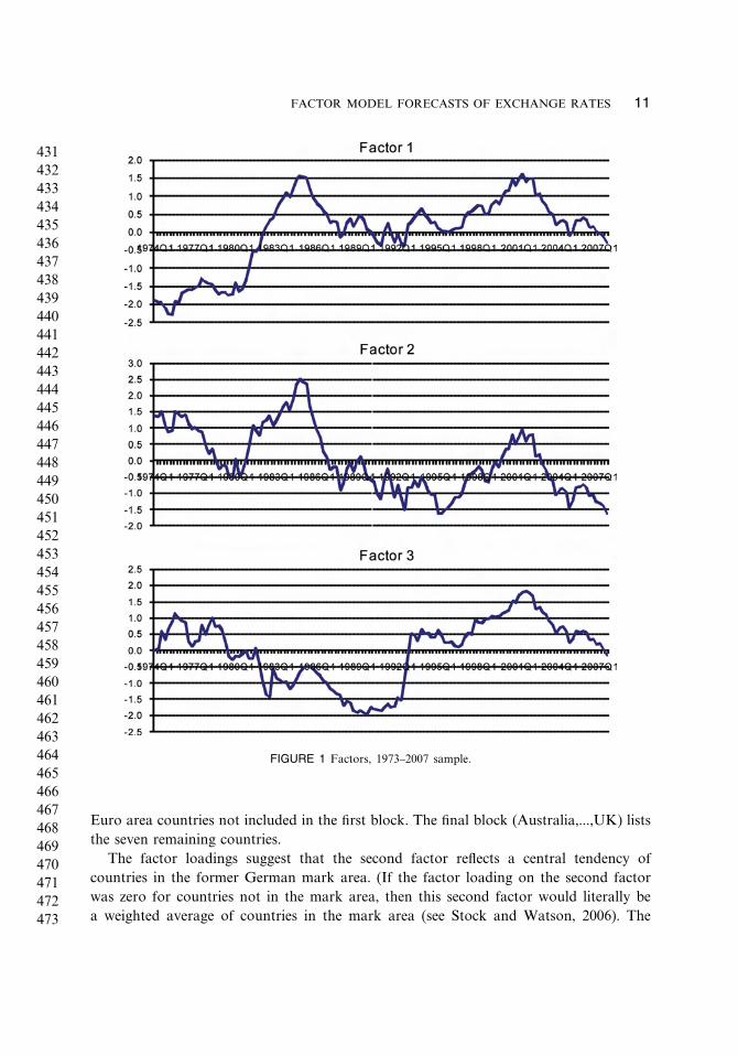
TABLE 4Results for Fit − sit, Varying Number of Factors r

Horizon h

No. of Factors® Sample/No. Currencies Statistic 1 4 8 12

1 long/N = 9 median U 1.011 1.037 1.083 1.154#U < 1 or (t > 1�282) 1(0) 1(0) 1(0) 1(0)



1 early/N = 17 median U 0.996 0.969 0.995 1.103#U < 1 or (t > 1�282) 9(3) 10(3) 9(1) 3(0)



1 late/N = 10 median U 1.021 1.081 1.179 1.294#U < 1 or (t > 1�282) 1(0) 1(0) 1(0) 1(1)



Notes: 1. The results for r = 2 in this table repeat, for convenience, those for Fit − sit in Table 3. 2. Seenotes to Table 3.

(the exceptions in this case being Fit − sit + PPP for h=1 and 4, and Fit − sit + monetaryfor h = 1). In the late sample, however, 9 of the 16 medians are above 1, with themodels doing consistently better than a random walk (median U < 1) at 8 and 12 quarterhorizons. Note in particular that in this sample, 8 of the 10 U-statistics were below 1 forFit − sit and Fit − sit + monetary, and 9 or 10 were below 1 for Fit − sit + PPP.

Table 4 illustrates how varying the number of factors affects the simplest model, thatof Fit − sit; results for models that include Taylor rule, monetary or PPP fundamentals aresimilar. The table indicates that for the long sample, r = 3 performs a little better and ther = 1 model a little worse than does the r = 2 model presented in Table 3. In the earlysample, the r = 2 model is the worst performing; the r = 1 model is the best performing.In the late sample, the r = 2 and r = 3 models perform similarly, with the r = 1 modelperforming distinctly more poorly than either of the other models.

To depict visually what underlies a U-statistic of various values, let us focus on theUnited Kingdom, r = 3 factors, model = Fit − sit, long sample. The U-statistics happento be 1.003 (h = 1), 0.996 (h = 4), 0.979 (h = 8), and 0.969 (h = 12). (These U-statistics,as well as other individual currency U-statistics discussed below, are not reported in anytable.) A scatter plot of the recursive estimates of Fit − sit, and of the subsequent h-quarter

603604605606607608609610611612613614615616617618619620621622623624625626627628629630631632633634635636637638639640641642643644645


FIGURE 2 Forecast errors and realizations, U.K., r = 3 factors, model = Fit − sit , long sample.

change in the exchange rate, is in Fig. 2. The values of 0.979 and 0.968 for the U-statisticsfor h = 8and h = 12 imply a reduction in RMSPE relative to a no-change forecast ofabout 2–3%. Despite the seemingly small reduction, the figures for h = 8 and h = 12depict an unambiguously positive relation between the deviation from the factor Fit − sitand the subsequent change in the exchange rate. On the other hand, there clearly is a lotof variation in a relation that is positive on average.

Our predictions fared especially poorly for the Japanese yen, which generally had oneof the highest U-statistics in each sample and model. For example, the U-statistics forJapan, r = 2 factors, model = Fit − sit, long sample were 1.008 (h = 1), 1.051 (h = 4),1.085 (h = 8), and 1.160 (h = 12). That the yen does not quite fit into the same moldas the other currencies in our study is perhaps suggested by the large negative weight

646647648649650651652653654655656657658659660661662663664665666667668669670671672673674675676677678679680681682683684685686687688

16 C. ENGEL ET AL.

of −0.55 for the yen on the first factor (see Table 2). In the late sample, continentalcurrencies (Denmark, Norway, Sweden, Switzerland) and, to a lesser extent, the Eurowere generally well predicted by our models. For example, the figures for the Eurofor r = 2 factors, model = Fit − sit, late sample were 1.009 (h = 1), 1.015 (h = 4), 0.939(h = 8), and 0.816 (h = 12).

Over all specifications and horizons (1, 2 and 3 factors; long, early and late samples;horizons of 1, 4, 8 and 12 quarters), only the Fit − sit + PPP model had median U-statistics less than 1 in over 50 percent of the forecasts.

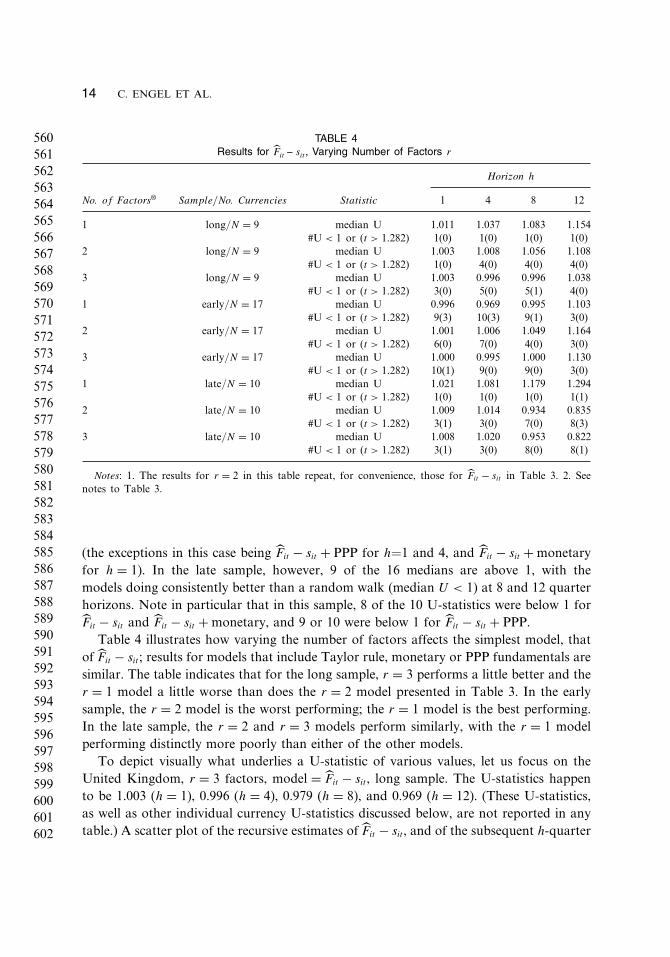
To further check the sensitivity of our results to particular sample periods, Figure 3graphs recursively computed U-statistics for the h = 1 and h = 8 horizons, r = 2 factors,model = Fit − sit, for the United Kingdom and Japan, long sample, and the Euro, latesample. The initial value in the graphs—1987:1 (h = 1) or 1988:4 (h = 8) for the U.K.and Japan, 1999:2 (h = 1) or 2001:1 (h = 8) for the Euro—is computed from a singleobservation. The number of observations used in computing the U-statistics increasesthrough the sample with the number of observations used to compute the final value in2007:4 given in the relevant entries of panel A of Table 1: 84 (h = 1) and 77 (h = 8) forthe UK and Japan, and 35 (h = 1) and 28 (h = 8) for the Euro. The final values in thegraphs, in 2007:4, is the one reported in the tables and the text above. For example, 0.939for Euro, h = 8, is the final value for the Euro in the h = 8 graph. Note that the verticalscale is different for the h = 1 and h = 8 graphs.

Of course, the initial values in the graphs fluctuate quite a bit. But once a couple ofyears worth of observations have been accumulated, the values settle down. We see thatthe figures reported in the tables and text and discussed above are representative: apartfrom start up values computed from few observations, there is no apparent sensitivityto sample. In the h = 1 graph, U-statistics consistently are near 1, and generally areabove 1. This indicates that for one quarter ahead forecasts, the average squared valueof the forecast from the factor model generally is slightly above that of a random walkmodel. In the h = 8 graph, we see that the poor performance of our factor model thatwe noted above for Japan obtains for the whole sample; the modestly good performancethat we noted for the United Kingdom also obtains for most of the sample; and the goodperformance for the Euro obtains consistently once the effects of initial observations havebeen averaged out.

6. ROBUSTNESS

We checked the robustness of these results in a number of dimensions.

1. We estimated by principal components rather than by maximum likelihood. Overall,results were comparable, with one technique doing a little better (occasionally, a lotbetter) in one specification and the other doing a little better (occasionally, a lotbetter) in other specifications. We also used the British pound rather than the U.S.

689690691692693694695696697698699700701702703704705706707708709710711712713714715716717718719720721722723724725726727728729730731


FIGURE 3 Recursive U-statistics, r = 2 factors, model = Fit − sit , U.K., Japan, and Euro.

732733734735736737738739740741742743744745746747748749750751752753754755756757758759760761762763764765766767768769770771772773774

18 C. ENGEL ET AL.

dollar as the base currency. Estimation was by maximum likelihood. Here, results werecomparable for the early sample, somewhat worse for the long and late samples.

A detailed summary of the robustness checks is in an appendix available on request.To illustrate, let us take two lines from Table 3, and present analogous results fromprincipal components estimation, and from estimation with the British pound as thebase currency. These lines are chosen because they are representative:

h = 1 h = 4 h = 8 h = 12Fit − sit, early/N = 17,

maximum likelihood, U.S. dollar (Table 3) 6(0) 7(0) 4(0) 3(0) (6.1a)Fit − sit, early/N = 17,

principal components, U.S. dollar 4(2) 4(3) 7(4) 8(2) (6.1b)Fit − sit, early/N = 17,

maximum likelihood, British pound 6(1) 6(1) 4(2) 4(0) (6.1c)Fit − sit + PPP, late/N = 10,

maximum likelihood, U.S. dollar (Table 3) 4(0) 5(0) 8(0) 9(5) (6.2a)Fit − sit + PPP, late/N = 10,

principal components, U.S. dollar 3(3) 3(3) 7(2) 9(4) (6.2b)Fit − sit + PPP, late/N = 10,

maximum likelihood, British pound 3(0) 1(0) 1(0) 1(0) (6.2c)

We see in (6.1a) and (6.1b) that in terms of the number of U-statistics less than one,principal components improves over maximum likelihood at h = 12 (8 versus 3 U-statistics less than 1), while the converse is true at h = 4 (4 versus 7 U-statistics lessthan 1). Results for the British pound in (6.1c) similarly are better at some horizons,worse at other horizons. We see in (6.2a) and (6.2b) that principal components andmaximum likelihood generate very similar numbers, while (6.2c) illustrates that withthe British pound as the base currency, results degrade for the late sample.

2. We also computed a utility based comparison of our factor models relative to therandom walk. Our approach is stimulated by that of West et al. (1993), who consideralternative models for conditional volatility in contrast to our comparison of modelsfor conditional means. We consider an investor with a one period mean-variance utilityfunction, allocating wealth between U.S. and foreign one period debt that is nominallyriskless in own currency. Suppose that a given one of our factor models produceshigher expected utility than does the random walk. We ask, what fraction of wealthwould the investor be willing to give up to use our model rather than a random walkto forecast exchange rates? Of course, if the random walk forecasts better, we ask thesame question, but in our tables present the result with a negative sign. We let �UF and�URW denote utility gains from use of the factor and random walk models, cautioningthe reader that the �U here is not related to the “U” in Theil’s U.

Details are in the Appendix. Interest rate data on government debt were obtainedfrom Datastream, last day of the quarter. We calibrate our mean-variance utilityfunction so that it implies a coefficient of relative risk aversion of 1 at the initial wealth

775776777778779780781782783784785786787788789790791792793794795796797798799800801802803804805806807808809810811812813814815816817


TABLE 5

A. Wealth Sacrifice to use Higher Utility Model, for Fit − sit , Horizon h = 1, Two Factor Models

model

Taylor+ Mon+ PPP+Sample/No. Currencies Statistic Fit − sit Fit − sit Fit − sit Fit − sit

long/N = 9 median sacrifice | �UF > �URW 19 4 179 51median sacrifice | �URW > �UF –65 –134 –479 –112

#�UF > �URW 3 1 3 4

early/N = 17 median sacrifice | �UF > �URW 147 74 583 173median sacrifice | �URW > �UF –176 –120 –56 –1572

#�UF > �URW 12 6 9 15

late/N = 10 median sacrifice | �UF > �URW 110 92 280 95median sacrifice |�URW > �UF –21 –143 –1031 –196

#�UF > �URW 2 2 5 4

B. Results for Fit − sit , Monthly data, Two Factor Models

Horizon h

Sample/No. Currencies Statistic 1 12 24 36

long/N = 9 median U 1.002 1.005 0.975 0.974#U < 1 or (t > 1�282) 2(0) 3(0) 6(3) 6(5)

early/N = 17 median U 1.002 0.997 1.058 1.302#U < 1 or (t > 1�282) 6(0) 9(0) 3(1) 4(1)

late/N = 10 median U 1.002 1.006 0.979 0.985#U < 1 or (t > 1�282) 3(0) 4(1) 6(2) 6(3)

C. Full Sample Estimates of for Fit − sit , Two Factor Models

Horizon h

Sample/No. Currencies Statistic 1 4 8 12

long/N = 9 –0.008 –0.011 –0.040 –0.081std. error (0.003) (0.004) (0.012) (0.020)

early/N = 17 –0.009 –0.015 –0.047 –0.088std. error (0.005) (0.003) (0.009) (0.014)

late/N = 10 –0.007 –0.010 –0.041 –0.081std. error (0.004) (0.004) (0.011) (0.018)

Notes: 1. Consider a risk averse investor, with coefficient of relative risk aversion of 1, who uses eithera factor or random walk model to allocate his wealth across two assets whose returns are nominally safewhen measured in own currency. In Panel A, �UF > �URW means the factor model delivers higher expectedutility. The “median sacrifice” reports the fraction of wealth expressed in annualized basis points that suchan investor would be willing to give up to use the factor rather than random walk model (when �UF > �URW )or the random walk rather than the factor model (when �URW > �UF ). (The �U used here bears no relation tothe “U” in Theil’s U that is referenced in panel B of this Table and elsewhere in the paper.) See section 6 ofthe paper for additional detail. 2. Panel B presents estimates for monthly data comparable to the estimatesin the Fit − sit lines in Table 3. 3. Panel C presents estimates of from Eq. (3.5) in the case that � ≡ 0 (i.e.,the model is Fit − sit) and the number of factors is two.

818819820821822823824825826827828829830831832833834835836837838839840841842843844845846847848849850851852853854855856857858859860

20 C. ENGEL ET AL.

level. We answer “what fraction of wealth would the investor give up” in terms ofannualized basis points. Results for one quarter ahead forecasts and two factor modelsare in Table 5A. Comparable results for the mean squared error criterion are in theh = 1 column that runs down Table 3. The utility based and mean squared criteriaperform similarly in terms of whether a factor model performs better. For example,for the long sample, Table 5A indicates that the factor based model is preferred bythe utility criterion in 11 (= 3 + 1 + 3 + 4) of the 36 comparisons; we see in the h = 1column in the top four rows of Table 3 that the comparable figure is 8 of 36 for themean squared error criterion. For both criteria, the factor models are preferred in alarger fraction of comparisons in the early than in the long or late samples.

By both criteria, performance differences generally are small. Of the 24 performancefees in Table 5A, all but 5 are less than 200 basis points in absolute value, a comparisonthat is relevant since management fees typically run around 200 basis points. This isconsistent with the finding that at a one quarter horizon, the estimates of Theil’s Uwere generally very close to 1.

We conclude that by both statistical and utility based criteria, the differencesbetween factor models and the random walk are small at a one quarter horizon.

3. We repeated the mean squared error comparison using monthly data, for two factormodels, and horizons of 1, 12, 24, and 36 months. Results are in Table 5B. Comparablequarterly figures are in the three “Fit − sit” lines in Table 3. Results are qualitativelysimilar for the two frequencies. The factor model does especially well at the longhorizons in the late sample; performance differences are very small at shorter (1 and12 month) horizons.

4. Finally, in Table 5C we report point estimates and standard errors for the slopecoefficient in (3.5), for the model Fit − sit. Qualitatively, the results align with thoseof our out of sample tests, in that t-statistics tend to increase with the horizon.However, all but two of the t-statistics are significant at the five percent level (theexceptions being the early and late samples, h = 1). Thus, as is often the case, there ismore significance for a predictor with in-sample than with out-of-sample evidence. Weinterpret this as an endorsement of our decision to focus on out of sample analysis:we otherwise might have been unduly optimistic about the performance of our factormodel.

7. CONCLUSIONS

This first pass at extracting factors from the cross-section of exchange rates yielded mixedresults. Results for late samples (1999–2007) were promising, at least for horizons of 8or 12 quarters. With occasional exceptions for models that relied not only on factors butPPP fundamentals as well, other results suggested no ability to improve on a “no-change,”or random walk, forecast.

861862863864865866867868869870871872873874875876877878879880881882883884885886887888889890891892893894895896897898899900901902903


Late samples allow larger sample sizes for estimation of factors. While that may bepart of the reason for good results for late samples, that is not a sufficient conditionfor good results because our robustness checks found that the when the British pound isthe base currency, late samples perform worse than early samples. Indeed, it remains tobe seen whether our results for late samples are spurious. In any event, the frameworkhere can be extended in a number of ways. It would be desirable to allow differentslope coefficients across currencies, to allow more flexible specification of parametersin monetary and Taylor rule models, and to use a data dependent method of selectingthe number of factors. Such extensions are priorities for future work. It would also bedesirable to compare our predictions to, not only a random walk model, but to othermodels that have been compared to the random walk in earlier studies.

APPENDIX

In this Appendix, we describe the utility based calculation presented in Table 5A. Webegin with some notation. We drop the i subscript from the exchange rate st and othervariables for simplicity. Define

st = forecast of st+1; st = st for random walk,

st = factor model forecast for factor model; (A.1)

�2t = variance of st+1 as of time t, computed as t−1

t∑j=2

(sj − sj−1)2 for both models;

(A.2)

Rt+1,R∗t+1 = nominal return on one period nominal riskless debt in the U.S. and abroad;

(A.3)

�t+1 = R∗t+1 − Rt+1 − (st+1 − st) = ex-post return differential; (A.4)

�t = R∗t+1 − Rt+1 − (st − st) = ex-ante return differential. (A.5)

Let us tentatively assume that �t is positive, i.e., that when we use a given model forst, the expected return is higher abroad than in the U.S. The goal of a U.S. investor withinitial wealth W is to

maxf

EtUt+1 = Et[Wt+1 − 0�5�W 2t+1] s.t.

Wt+1 = W [f(R∗t+1 − �st+1) + (1 − f)Rt+1] = W (f�t+1 + Rt+1)� (A.6)

In solving for the optimal f , call it f ∗, set Et�t+1 = �t, Et�2t+1 = �2t + �2

t . Then,

f ∗ = 1 − �WRt+1

�W�t

�2t + �2t

� (A.7)

904905906907908909910911912913914915916917918919920921922923924925926927928929930931932933934935936937938939940941942943944945946

22 C. ENGEL ET AL.

Plug f ∗ back into EtUt+1. Rearrange, and the result is

EtUt+1 = [ct + dtEtut+1(�t+1, ��2t+1, �t, �2t )]W , (A.8)

ct = Rt+1 − �5�WR2t+1, dt = (1 − �WRt+1)

2/�W ,

ut+1(·) = �

�2t + �2t

(�t+1 − �5

�t

�2t + �2t

�2t+1

),

Etut+1(·) = �

�2t + �2t

(Et�t+1 − �5

�

�2t + �2t

Et�2t+1

)�

We compute the total utility of a U.S. investor using one of our models as the sumover t of ct + dtut+1 in those periods in which �t is positive, i.e., we compute the utilitygains for a U.S. investor only in those quarters in which the foreign return is expectedto be higher than the U.S. return (otherwise, the U.S. investor puts all wealth into Rt+1

because this is a safe asset). We compute the total utility of a foreign investor (with signsof returns reversed) over those periods in which �t is negative. We average the two utilitiesover P periods of predictions to get an average utility based measure of the quality of oneof the models.

Let �UF and �URW be the average utility measures that result from a factor model and therandom walk model. We report the fraction of wealth that our investor would be willingto give up to use the higher utility model, expressed at an annualized rate, in basis points.When �UF > �URW , Table 5A reports 40, 000 × (1 − �URW/�UF ). When �URW > �UF , the tablereports −40, 000 × (1 − �UF/�URW ). The factor of 4 converts quarterly to annual points,while the factor of 10,000 converts to basis points.

For quadratic utility (A.6), the coefficient of relative risk is �W/(1 − �W ). We fix thisvalue at 1.

ACKNOWLEDGMENTS

We thank Wallice Ao, Roberto Duncan, Lowell Ricketts, and Mian Zhu for exceptionalresearch assistance; the editor, two anonymous referees and seminar audiences at theEuropean Central Bank and the IMF for helpful comments. The Additional Appendixthat is referenced in the paper is available on request from the authors.

FUNDING

We thank the National Science Foundation for financial support.

947948949950951952953954955956957958959960961962963964965966967968969970971972973974975976977978979980981982983984985986987988989


REFERENCES

Bacchetta, P., van Wincoop, E. (2006). Can information heterogeneity explain the exchange rate determinationpuzzle? American Economic Review 96(3):552–576.

Bai, J. (2004). Estimating cross-section common stochastic trends in nonstationary panel data. Journal of Q6Econometrics 137–183.

Benigno, G., Benigno, P. (2006). Exchange rate determination under interest rate rules. Manuscript, LondonSchool of Economics.

Bulut, L., Maasoumi, E. (2012). Predictability and specification in models of exchange rate determination. Q7Forthcoming in Recent Advances and Future Directions in Causality, Prediction, and SpecificationAnalysis (In honor of Halbert White). Springer.

Cheung, Y.-W., Chinn, M., Garcia Pascual, A. (2005). Empirical exchange rate models of the Nineties: Areany fit to survive? Journal of International Money and Finance 24:1150–1175.

Clark, T. E., West, K. D. (2006). Using out-of-sample mean squared prediction errors to test the Martingaledifference hypothesis. Journal of Econometrics 135(1–2):155–186.

Clark, T. E., West, K. D. (2007). Approximately normal tests for equal predictive accuracy in nested models.Journal of Econometrics 138(1):291–311.

Diebold, F. X., Gardeazabal, J., Yilmaz, K. (1994). On cointegration and exchange rate dynamics. Journalof Finance XLIX:727–735.

Engel, C., West, K. D. (2005). Exchange rates and fundamentals. Journal of Political Economy 113:485–517.Engel, C., West, K. D. (2006). Taylor rules and the Deutschemark-Dollar real exchange rate. Journal of

Money, Credit and Banking 38:1175–1194.Engel, C., Mark, N. M., West, K. D. (2008). Exchange rate models are not as bad as you think. In: Acemoglu,

D., Rogoff, K., Woodford, M., eds. NBER Macroeconomics Annual, 2007. Chicago: University of ChicagoPress, pp. 381–443.

Groen, J. J. J. (2005). Exchange rate predictability and monetary fundamentals in a small multi-country panel.Journal of Money, Credit and Banking 37:495–516.

Groen, J. J. J. (2006). Fundamentals based exchange rate prediction revisited. Manuscript, Bank of England.Hubrich, K., West, K. D. (2010). Forecast comparisons for small nested model sets. Journal of Applied

Econometrics 25:574–594.Ho, M. S., Sørensen, B. E. (1996). Finding cointegration rank in high dimensional systems using the Johansen

test: An illustration using data based Monte Carlo simulations. Review of Economics and Statistics726–732.

Mark, N. A. (1995). Exchange rates and fundamentals: Evidence on long-horizon predictability. AmericanEconomic Review 85:201–218.

Mark, N. A. (2001). International Macroeconomics and Finance: Theory and Empirical Methods. New York:Blackwell.

Mark, N. A. (2008). Changing Monetary policy rules, learning and real exchange rate dynamics. Manuscript,University of Notre Dame.

Mark, N. A., Sul, D. (2001). Nominal exchange rates and monetary fundamentals: Evidence from a smallPost-Bretton Woods sample. Journal of International Economics 53:29–52.

Meese, R. A., Rogoff, K. (1983a). Empirical exchange rate models of the Seventies: Do they fit out of sample?Journal of International Economics 14:3–24.

Meese, R. A., Rogoff, K. (1983b). The out-of-sample failure of empirical exchange rate models: Samplingerror or misspecification. In: Frenkel, J. A., ed. Exchange Rates and International Macroeconomics.Chicago: University of Chicago Press.

Molodtsova, T., Papell, D. (2008). Taylor rules with real-time data: A Tale of two countries and one exchange.Journal of Monetary Economics 55:S63–S79.

Rapach, D. E., Wohar, M. E. (2002). Testing the Monetary model of exchange rate determination: New Q8evidence from a century of data. Journal of International Economics 58:359–385.

Rapach, D. E., Wohar, M. E. (2004). Testing the Monetary model of exchange rate determination: A closerlook at panels. Journal of International Money and Finance 23(6):841–865.

990991992993994995996997998999100010011002100310041005100610071008100910101011101210131014101510161017101810191020102110221023102410251026102710281029103010311032

24 C. ENGEL ET AL.

Stock, J. H., Watson, M. W. (2006). Forecasting with many predictors. In: Elliott, G., Granger, C. W. J.,Timmermann, A., eds. Handbook of Economic Forecasting. Vol. 1. Amsterdam: Elsevier, pp. 515–550.

West, K. D. (1996). Asymptotic inference about predictive ability. Econometrica 64:1067–1084.West, K. D. (2006). Forecast evaluation. In: Elliott, G. Granger, C. W. J., Timmerman, A. eds. Handbook

of Economic Forecasting. Vol. 1. Amsterdam: Elsevier, pp. 100–134.West, K. D., Edison, H. J., Cho, D. (1993). A utility based comparison of some models of exchange rate

volatility. Journal of International Economics 35.

factormodelforecastsofexchangerates - sscc - homecengel/publishedpapers/factorforecasts.pdf · that...

Documents