factors that impact direct democracy and voter turnout
TRANSCRIPT

UNLV Theses, Dissertations, Professional Papers, and Capstones
December 2018
Factors that Impact Direct Democracy and Voter Turnout: Factors that Impact Direct Democracy and Voter Turnout:
Evidence from a National Study on American Counties Evidence from a National Study on American Counties
Michael Joseph Biesiada
Follow this and additional works at: https://digitalscholarship.unlv.edu/thesesdissertations
Part of the Public Administration Commons
Repository Citation Repository Citation Biesiada, Michael Joseph, "Factors that Impact Direct Democracy and Voter Turnout: Evidence from a National Study on American Counties" (2018). UNLV Theses, Dissertations, Professional Papers, and Capstones. 3402. http://dx.doi.org/10.34917/14279037
This Dissertation is protected by copyright and/or related rights. It has been brought to you by Digital Scholarship@UNLV with permission from the rights-holder(s). You are free to use this Dissertation in any way that is permitted by the copyright and related rights legislation that applies to your use. For other uses you need to obtain permission from the rights-holder(s) directly, unless additional rights are indicated by a Creative Commons license in the record and/or on the work itself. This Dissertation has been accepted for inclusion in UNLV Theses, Dissertations, Professional Papers, and Capstones by an authorized administrator of Digital Scholarship@UNLV. For more information, please contact [email protected].
FACTORS THAT IMPACT DIRECT DEMOCRACY AND VOTER TURNOUT:
EVIDENCE FROM A NATIONAL STUDY ON AMERICAN COUNTIES
By
Michael Joseph Biesiada
Bachelor of Science in Business Administration – Marketing University of Nevada, Las Vegas
2008
Bachelor of Science in Business Administration – Management Information Systems University of Nevada, Las Vegas
2009
Master of Education – Higher Education University of Nevada, Las Vegas
2013
A dissertation submitted in partial fulfillment of the requirements for the
Doctor of Philosophy – Public Affairs
School of Public Policy and Leadership Greenspun College of Urban Affairs
The Graduate College
University of Nevada, Las Vegas December 2018

Copyright by Michael Joseph Biesiada, 2018
All Rights Reserved

ii
Dissertation Approval
The Graduate College The University of Nevada, Las Vegas
September 20, 2018
This dissertation prepared by
Michael Biesiada
entitled
Factors That Impact Direct Democracy and Voter Turnout: Evidence from A National Study On American Counties
is approved in partial fulfillment of the requirements for the degree of
Doctor of Philosophy – Public Affairs School of Public Policy and Leadership
Jayce Farmer, Ph.D. Kathryn Hausbeck Korgan, Ph.D. Examination Committee Chair Graduate College Interim Dean
Jessica Word, Ph.D. Examination Committee Member
Jaewon Lim, Ph.D. Examination Committee Member
Daniel Lee, Ph.D. Graduate College Faculty Representative

iii
Abstract
This dissertation examines factors that impact citizen initiatives and voter turnout. The
dissertation contains two parts that build upon each other with fitting theoretical frameworks.
The first part investigates the decision for a county government to permit citizen initiatives. This
part applies new institutionalism theory as a framework to examine county governance,
autonomy, and decision-making. County governments play a vital role in American politics, yet
little is known about why some counties permit citizen initiatives while others do not. I address a
gap in the literature that focuses on policy outcomes that vary at the county-level due to election
laws. Therefore, this study is one of the first empirical works to examine the institutional
arrangements that impact the enactment of citizen initiatives at the county-level. To investigate
counties that permit the citizen initiative, I collect data from a national dataset on American
counties from the International City/County Management Association (ICMA) 2014 Survey,
U.S. Department of Education, American Community Survey (ACS), U.S. Census Bureau,
Community Development Financial Institutions Fund (CDFI Fund), and the 2013 NACO state
report. Using a logistic model, I find cross-sectional evidence that the citizen initiative has a high
association with the commission and council-elected governments for U.S. counties surveyed in
46 states. The findings suggest that elected representatives have a place in county government
structure, citizens within certain county governments can use the initiative as a safeguard against
political malfeasance, and elected representatives can use the initiative to engage public opinion.
In addition, the first part of this dissertation provides evidence that counties afforded the home
rule authority are more likely associated with the initiative, high-income counties are more likely
associated with the initiative, and, conversely, higher educated counties are less likely associated
with the initiative.

iv
The second part of this dissertation investigates the impact of citizen initiatives on voter
turnout. This part uses participatory democratic theory as a lens to examine the attitudes and
interests of citizens in the context of voter turnout. Therefore, this part is one of the first
empirical works that contributes to the literature by determining the effect of uncharted county
and state-level factors on county voter turnout. To conduct an analysis on voter turnout, I collect
data from a national dataset on American counties from the International City/County
Management Association (ICMA) 2014 Survey, American Community Survey (ACS), U.S.
Atlas of Elections, Community Development Financial Institutions Fund (CDFI) Fund,
Ballotpedia, and FairVote. Using both single-level and multilevel OLS models, I find cross-
sectional evidence that information costs put a burden on voters in U.S. counties surveyed in 23
states during the 2016 election. The findings suggest information cost for both county and state
initiatives can hinder voter participation, income inequality has a negative impact on county
turnout, and educated citizens care about voting. Along the way, I provide evidence that sorts out
competing claims on how citizen initiatives impact the rational voter.

v
Acknowledgements
I have spent my entire academic career at UNLV. I have numerous faculty, colleagues,
friends, and family to thank for completing a Ph.D. in Public Affairs at UNLV. This
acknowledgment section will only be a brief list of my more recent experiences, but I hope to
convey my sincere appreciation for the UNLV community.
As chair of my dissertation, Dr. Jayce Farmer was incredibly instrumental in the
development and completion of this project. Even with a wide range of department
responsibilities, he took me on as a student because our research interests were so closely
aligned. Starting from our first meeting, Dr. Farmer was very giving of his time to discuss how
my research questions lined up with the current public administration literature. We moved
swiftly through the many steps that it takes to build a credible dissertation project. It was only a
short time after that we would be drawing out diagrams and mapping out techniques to analyze
my data. As a result, I owe a great debt of gratitude for his support throughout this dissertation
project. Moreover, Dr. Farmer was incredibly supportive of my exposure to various university
activities that included presenting my research to public forums, serving as a graduate
ambassador, and helping expand my teaching activities. I am incredibly grateful that he is a
colleague studying public policy issues at UNLV.
I want to thank Dr. Jessica Word for her time and support. In particular, Dr. Word played
a key role by writing letters of support on my behalf even before I started working with Dr.
Farmer. Dr. Word offered many insights that pushed the scope of this dissertation project to
press the assumptions and insights. Likewise, I thank Dr. Jaewon Lim for taking the time to think
about my research questions and models together. He always helped me clarify my approach in
using various models incorporated in this dissertation. I want to thank Dr. Daniel Lee for serving
vi
as an outside representative, who was also very giving of his time. Dr. Lee is a careful thinker,
who offered countless ways to improve the value of my dissertation. Dr. Lee was always helpful
in discussing a range of issues, from the political implications to breaking down complicated
areas into neatly defined parts.
I also would like to thank Dr. Helen Neill. Dr. Neill played a pivotal part in my early
experiences as a Ph.D. student. Dr. Neill was instrumental in shaping and clarifying my thinking
on important public policy issues. These early conversations with Dr. Neil would ultimately lead
me to my final dissertation topic. I want to thank Dr. Lee Bernick. Once I settled on a topic, Dr.
Bernick was always happy to take time out to discuss the implications of my project and offer
thoughtful feedback. I thank Dr. Christopher Stream, who was always there to offer friendly
words of advice that would lift my spirits. I also thank Dr. Victoria Rosser, Dr. Harriet Barlow,
and Dr. Tiberio Garza, who have been incredibly important supporters of mine since my early
days at UNLV.
I am grateful to the UNLV Graduate College and the Graduate Professional Student
Association. In particular, I am thankful for the support from Dean Kathryn Korgan and Valarie
Burke, especially while I served as a UNLV graduate ambassador. I want to thank UNLV
Librarian Patrick Griffis for his time and effort. He was always willing to lend a helping hand in
tracking down data and verifying sources. I also want to thank my very dear friend, Dr. Andrea
Buenrostro for her support and loving encouragement. Lastly, I am very grateful to my parents
and sister. Their unconditional support made this achievement possible. I owe everything to my
wonderful family.

vii
Dedication
I dedicate this dissertation to dad, mom, and Ani. Your support made it all possible.

viii
Table of Contents
Abstract .......................................................................................................................................... iii
Acknowledgements ......................................................................................................................... v
Dedication ..................................................................................................................................... vii
List of Tables ................................................................................................................................. xi
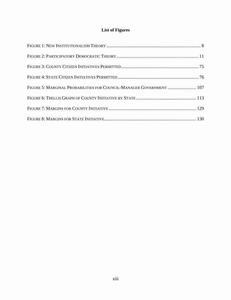
List of Figures .............................................................................................................................. xiii
List of Equations .......................................................................................................................... xiv
List of Abbreviations .................................................................................................................... xv
Chapter 1: Introduction ................................................................................................................... 1
Purpose of Study ......................................................................................................................... 1
Chapter 2: Literature Review .......................................................................................................... 5
Theoretical Frameworks .............................................................................................................. 5
New Institutionalism Theory ................................................................................................... 5
Participatory Democratic Theory ............................................................................................ 9
Direct Democracy ..................................................................................................................... 12
Overview ............................................................................................................................... 12
Benefits of Citizen Initiatives ................................................................................................ 15
County vs. State Citizen Initiatives ....................................................................................... 17
Part I: The Link Between County Governments and Direct Democracy .................................. 18
County Citizen Initiatives ...................................................................................................... 18
County Government Overview .............................................................................................. 19
Commission Governments .................................................................................................... 25
Reformed Governments ......................................................................................................... 30

ix
Home Rule Charter ................................................................................................................ 39
Socioeconomic Variables ...................................................................................................... 41
Control Variables ................................................................................................................... 45
Direct Democracy: From Outcome to Predictor ................................................................... 48
Part II: The Impact of Direct Democracy on Voter Turnout ..................................................... 50
Voter Turnout ........................................................................................................................ 50
County-Level Variables ......................................................................................................... 52
State-Level Variables ............................................................................................................ 55
Control Variables ................................................................................................................... 60
Summary ................................................................................................................................... 64
Chapter 3: Data and Methods ....................................................................................................... 68
Data Operationalization ............................................................................................................. 68
Data Identification ..................................................................................................................... 72
State Breakdown of Citizen Initiatives ...................................................................................... 75
Methods and Models ................................................................................................................. 77
Chapter 4: Empirical Results ........................................................................................................ 84
Part I: Government Structure Model ......................................................................................... 84
Model Diagnostics ................................................................................................................. 84
Descriptive Statistics ............................................................................................................. 90
Logistic Model 1 Interpretations ........................................................................................... 92
Logistic Model 2 and 3 Interpretations ................................................................................. 95
Logistic Model 4 and 5 Interpretations ................................................................................. 97
Logistic Model Results .......................................................................................................... 99

x
Goodness of Fit Test ............................................................................................................ 105
Council-Manager Predictions .............................................................................................. 105
Part II: Voter Turnout Model .................................................................................................. 108
Model Diagnostics ............................................................................................................... 108
Descriptive Statistics ........................................................................................................... 111
Trellis Graph by State .......................................................................................................... 112
Likelihood Ratio Test .......................................................................................................... 114
Multilevel Results ................................................................................................................ 115
Intraclass Correlation ........................................................................................................... 118
AIC and BIC Test ................................................................................................................ 120
Single-Level Model 1 Interpretations .................................................................................. 121
Single-Level Model 2 Interpretations .................................................................................. 125
Single-Level Results ............................................................................................................ 126
Initiative Predictions ............................................................................................................ 128
Summary ................................................................................................................................. 131
Chapter 5: Conclusions ............................................................................................................... 132
Lessons Learned ...................................................................................................................... 132
Limitations .............................................................................................................................. 135
Future Policy ........................................................................................................................... 136
Appendix A: MLM and Single-Level Model Comparison ......................................................... 139
References ................................................................................................................................... 141
Curriculum Vitae ........................................................................................................................ 156

xi
List of Tables
TABLE 1: FORM OF GOVERNMENT AND CITIZEN INITIATIVE EXPECTATIONS ................................. 38
TABLE 2: GOVERNMENT STRUCTURE | DIRECT DEMOCRACY DATA IDENTIFICATION .................... 73
TABLE 3: DIRECT DEMOCRACY | VOTER TURNOUT DATA IDENTIFICATION ................................... 74
TABLE 4: GOVERNMENT STRUCTURE FREQUENCIES ...................................................................... 86
TABLE 5: GOVERNMENT STRUCTURE CHI-SQUARED TESTS ........................................................... 87
TABLE 6: GOVERNMENT STRUCTURE MODEL MULTICOLLINEARITY RESULTS .............................. 89
TABLE 7: GOVERNMENT STRUCTURE CORRELATIONS ................................................................... 90
TABLE 8: GOVERNMENT STRUCTURE DESCRIPTIVE STATISTICS .................................................... 91
TABLE 9: GOVERNMENT STRUCTURE MODEL 1 RESULTS .............................................................. 99
TABLE 10: GOVERNMENT STRUCTURE MODEL 2 RESULTS .......................................................... 100
TABLE 11: GOVERNMENT STRUCTURE MODEL 3 RESULTS .......................................................... 101
TABLE 12: GOVERNMENT STRUCTURE MODEL 4 RESULTS .......................................................... 102
TABLE 13: GOVERNMENT STRUCTURE MODEL 5 RESULTS .......................................................... 103
TABLE 14: GOVERNMENT STRUCTURE COEFFICIENT INTERPRETATIONS ..................................... 104
TABLE 15: COUNCIL-MANAGER PREDICTION .............................................................................. 107
TABLE 16: VOTER TURNOUT MULTICOLLINEARITY RESULTS ...................................................... 109
TABLE 17: VOTER TURNOUT CORRELATIONS .............................................................................. 110
TABLE 18: VOTER TURNOUT DESCRIPTIVE STATISTICS ............................................................... 112
TABLE 19: VOTER TURNOUT MULTILEVEL MODEL RESULTS ...................................................... 117
TABLE 20: INTRACLASS CORRELATION COEFFICIENTS ................................................................ 120
TABLE 21: VOTER TURNOUT AIC AND BIC RESULTS .................................................................. 121
TABLE 22: VOTER TURNOUT SINGLE-LEVEL MODEL RESULTS ................................................... 126

xii
TABLE 23: VOTER TURNOUT SINGLE-LEVEL MODEL 2 RESULTS ................................................ 127
TABLE 24: COUNTY AND STATE PREDICTIVE MARGINS ............................................................... 131
TABLE 25: MLM AND SINGLE-LEVEL MODEL COMPARISON RESULTS ........................................ 140
xiii
List of Figures
FIGURE 1: NEW INSTITUTIONALISM THEORY ................................................................................... 8
FIGURE 2: PARTICIPATORY DEMOCRATIC THEORY ........................................................................ 11
FIGURE 3: COUNTY CITIZEN INITIATIVES PERMITTED .................................................................... 75
FIGURE 4: STATE CITIZEN INITIATIVES PERMITTED ....................................................................... 76
FIGURE 5: MARGINAL PROBABILITIES FOR COUNCIL-MANAGER GOVERNMENT ......................... 107
FIGURE 6: TRELLIS GRAPH OF COUNTY INITIATIVE BY STATE ..................................................... 113
FIGURE 7: MARGINS FOR COUNTY INITIATIVE ............................................................................. 129
FIGURE 8: MARGINS FOR STATE INITIATIVE ................................................................................. 130

xiv
List of Equations
EQUATION 1: GOVERNMENT STRUCTURE MODEL .......................................................................... 80
EQUATION 2: VOTER TURNOUT MODEL ......................................................................................... 83
EQUATION 3: LIKELIHOOD RATIO TEST ....................................................................................... 115
EQUATION 4: INTRACLASS CORRELATION COEFFICIENT .............................................................. 118
EQUATION 5: PROBABILITY OF VOTING ....................................................................................... 123

xv
List of Abbreviations
Initiatives Refers to citizen initiatives (a form of direct democracy in the United States) DD Direct Democracy
ICMA International City/County Management Association
ACS American Community Survey
CDFI Fund Community Development Financial Institutions Fund
VEP Voting Eligible Population
VAP Voting Age Population
OLS Ordinary Least Squares
MLE Maximum Likelihood Estimation
SLM Single-Level Model
MLM Multilevel Model

1
Chapter 1: Introduction
Purpose of Study
The first part of this study examines the direct democracy mechanism scholars refer to as
the citizen initiative. Citizen initiatives allow voters to participate in the lawmaking process,
often bypassing their state legislator with the intent of improving government performance
(Matsusaka, 2005). This study explores the relation between government structure and citizen
initiatives in American counties. The issue at hand is determining whether forms of county
governments make institutional decisions that result in different outcomes for enacting the
citizen initiative.
In the late nineteenth and early twentieth centuries, the United States witnessed the rise of
populist and progressive movements that called for a direct democracy reform (Givel, 2009;
Lawrence, Donovan, & Bowler, 2009). This history led to many changes that currently inform
the modern institutional arrangement between county government and direct democracy. As
Matsusaka (2005) notes, citizen initiatives have been driving policy change on numerous topics
that include affirmative action, municipal debt, and minimum wage laws. Along these lines,
many scholars have argued that citizen initiatives enable citizens to counteract special interest
groups that can be harmful to public policy (Boehmke, 2005; Matsusaka, 2005; Tolbert, McNeal,
& Smith, 2003).
State rules permit counties to decide whether to incorporate citizen initiatives
(Arceneaux, 2002), but it is currently unknown which counties decide to enact these policies at
the county-level. Thus, there is a wide variation of counties that decide to permit citizen
initiatives within the American states. Likewise, little research has delved into the theoretical
nature of examining institutional arrangements at the county-level. As DeSantis & Renner

2
(1996) point out, examining public policy outcomes as a result of county structures has been
mostly anecdotal. As a result, despite the increasing demands of county governments, there is
limited research on their role in permitting citizen initiatives.
The purpose of part one of this dissertation is to bridge the gap in county government
policy research in several ways. First, part one is important because the devolution of power
from the federal to subnational levels of government has caused counties, “the forgotten level of
government,” to become key players in the public process (Pink-Harper, 2016). Second, this
study builds on the work of McCabe & Feiock (2005), which proposes that nested institutional
levels have an impact on public policy outcomes. Third, it extends the work of Park et al. (2010)
by analyzing the role of the county form of government in the policy formation process. Fourth,
the public opinion research by Dyck & Baldassare (2009) motivate this dissertation, which
shows solid evidence that voters care about citizen initiatives. In fact, many of the studies that
focus on the citizen initiative only use a select number of states (i.e., 10-15 see Coan & Holman,
2008) to estimate the impact on the policymaking process. Therefore, I capitalize on my fifth
point by conducting a national analysis on 46 states that permit the county initiative, and 23
states that permit the state initiative.
The second part of this dissertation analyzes voter turnout. In light of recent scholarly
research, the debate about predictors of voter turnout continues. A meta-analysis produced by
Stockemer (2017b) covering 130 articles between 2004 and 2013 on voter turnout asserts that the
evidence is inconclusive. Therefore, Stockemer suggests that determinants of turnout might be
more complex than the current theory and is more context dependent. This dependency can have
significant ramifications when considering the differences between county and state citizen
initiatives.
3
Part two focuses on extending the body of work on citizen initiatives at both the county
and state-levels as a predictor of voter turnout. This study is important because as Matsusaka
(2005) points out, citizen initiatives often reflect the desires of constituents most closely at the
county-level (A. D. Green, 2014). The literature has produced various research works focusing
on the impact of initiatives on state-level voter turnout (Childers & Binder, 2012; Damore et al.,
2012; Tolbert, Grummel, & Smith, 2001). The literature has found that states with initiatives on
the ballot have higher voter turnout over time (Tolbert, Grummel, & Smith, 2009). At the
county-level, Lubell, Feiock, & Ramirez (2005) analyzed how initiatives play a role in public
policy outcomes.
Nonetheless, there are several unanswered questions regarding how citizen initiatives
affect voter turnout at the county-level. Little research has investigated how initiatives impact
voter turnout at the county-level while accounting for state-level factors. It is unclear how special
interest contributions toward citizen initiatives on the ballot can influence county voter turnout.
Furthermore, within this context, it is unknown how factors impact county voter turnout such as
income inequality, poverty, and unemployment. Thus, this study is one of the first research
designs to address these unknowns by using a single-level and multilevel model to examine the
impact of county and state level initiatives on county-level voter turnout.
The purpose of part two is to address the overarching research question of whether citizen
initiatives increase voter turnout by using county-level and state-level variables of interest. This
study contributes to the body of knowledge on voter turnout in several ways. First, this study
uses voter turnout at the county-level to capture the local effect of citizen initiatives. Second, this
study uses the funding that went to support and oppose each citizen initiative at the state level,
whereas Tolbert et al. only use the expenditures that supported citizen initiatives. As a result, a

4
“magnitude” effect of citizen initiative funding captures the financial motivations of citizen
initiatives in the 2016 presidential election. Third, I capture the effect of unchartered
socioeconomic factors such as the percent of the population on food stamps, income inequality,
and educational attainment. Fifth, I use a less utilized multilevel but highly recommended (see
Primo, Jacobsmeier, & Milyo, 2007) design to study the impact of county and state level
variables (e.g., presidential campaign strategies) on voter turnout. Finally, this study applies the
overall research design to the most recent and highly contentious 2016 presidential election
while controlling for several well-researched variables e.g., past voter turnout and competitive
voter turnout.
The dissertation proceeds as follows. Chapter two discusses the historical significance of
the citizen initiative, the connection between county government and citizen initiatives in part
one, and the impact of citizen initiatives on voter turnout in part two. In chapter three, I describe
the data operationalization, data identification, state breakdown of citizen initiatives at both the
county and state levels, methods, and provide a formal description of the two models to carry out
the analyses. In chapter four, I consider findings that contribute to the public administration and
political science literatures regarding citizen initiatives. In chapter five, I discuss the implications
of this study and future research.

5
Chapter 2: Literature Review
Academic research on county governments and direct democracy has been scarce.
Rather, most of the literature has focused on county governments as service providers (Benton,
2002; Benton, 2005; DeSantis & Renner, 1996). This dissertation focuses on filling the scholarly
research gap between municipal and state governments by examining the use and application of
citizen initiatives. The following section on new institutionalism theory provides a framework to
analyze the relation between county form of government and citizen initiatives. Specifically, this
section explores the institutional dynamics that may reveal the theoretical foundations of why the
availability of citizen initiatives are more prevalent in a certain form of county government.
After explaining the current nature of citizen initiatives available at the county-level, I turn my
attention to focusing on why citizen initiatives are relevant for voter turnout. As such, I describe
the application of participatory democratic theory to voter turnout.
Theoretical Frameworks
New Institutionalism Theory
New institutionalism theory guides the first topic of this dissertation by showing how
politics and institutions impact government decision-making to enact citizen initiatives. More
precisely, the county charter derived from the home rule of the state affords certain authority to
county governments. These institutional rules often play a significant role in whether a county
government will incorporate as a commission government, or as seen in recent decades convert
to a reformed government.
County government forms have been linked to differences in policy orientations and
incentive structures that sought to empower and strengthen county government so it could play a
more active role than municipal governments (Choi, Bae, Kwon, & Feiock, 2010). More exactly,

6
the executive and legislative responsibilities are structured differently between the county
governments. This matters since Lubell et al. (2005) show that county legislative and executive
institutions act as mediators in local policy change. Furthermore, political actors at the national
level may have limited control over policies of the state and county governments (Choi et al.,
2010).
New institutionalism is a theoretical framework that focuses on how institutions effect
public policy outcomes, and in turn, society (Searing, 1991). As McCabe & Feiock (2005)
explain, new institutionalism in political science has returned scholarly attention to rules that
shape public policy outcomes. To put simply, McCabe et al. show that institutions matter, both at
the state and city levels. This study applies this same line of logic to address the issue of whether
county charters dictate the type of direct democracy mechanism available within each county,
and whether home rule at the state level has any effect on the outcome. In this regard, state home
rule allows political actors to establish their choice of governance structure at the county level.
The two main distinctions of government are the commission government and reformed
government structure. In this case, the reformed governments include the council-elected,
council-manager, and council-administrator structures. If a specific form of government
produces a higher probability of having a direct democracy mechanism, then the analysis would
provide evidence that there is an effect of county government structures and state home rules.
Moreover, the result would support the claim by Sonenshein & Hogen-Esch (2006), who point
out that government structure must reflect both public and private interest. If a specific form of
government has a high degree of association with the availability of the initiative, then that
government is more closely fulfilling Sonenshein’s proposition.

7
In politics, elected officials face high-powered incentives to please their constituency or
face defeat at the polls (McCabe & Feiock, 2005). Therefore, elected officials are more likely to
enact policies that resemble the median voter preferences except those representing reformed
governments (Farnham, 1987), and home rule only increases this likelihood (Turnbull & Geon,
2006). As such, due to high-powered incentives for elected officials (McCabe & Feiock, 2005),
the commission form of government may be more prompted to incorporate citizen initiatives.
Moreover, the nested level of institutional arrangements between state and county governments
provides an opportunity to study the incorporation of direct democracy mechanisms in the
presence of home rule and socioeconomic factors.
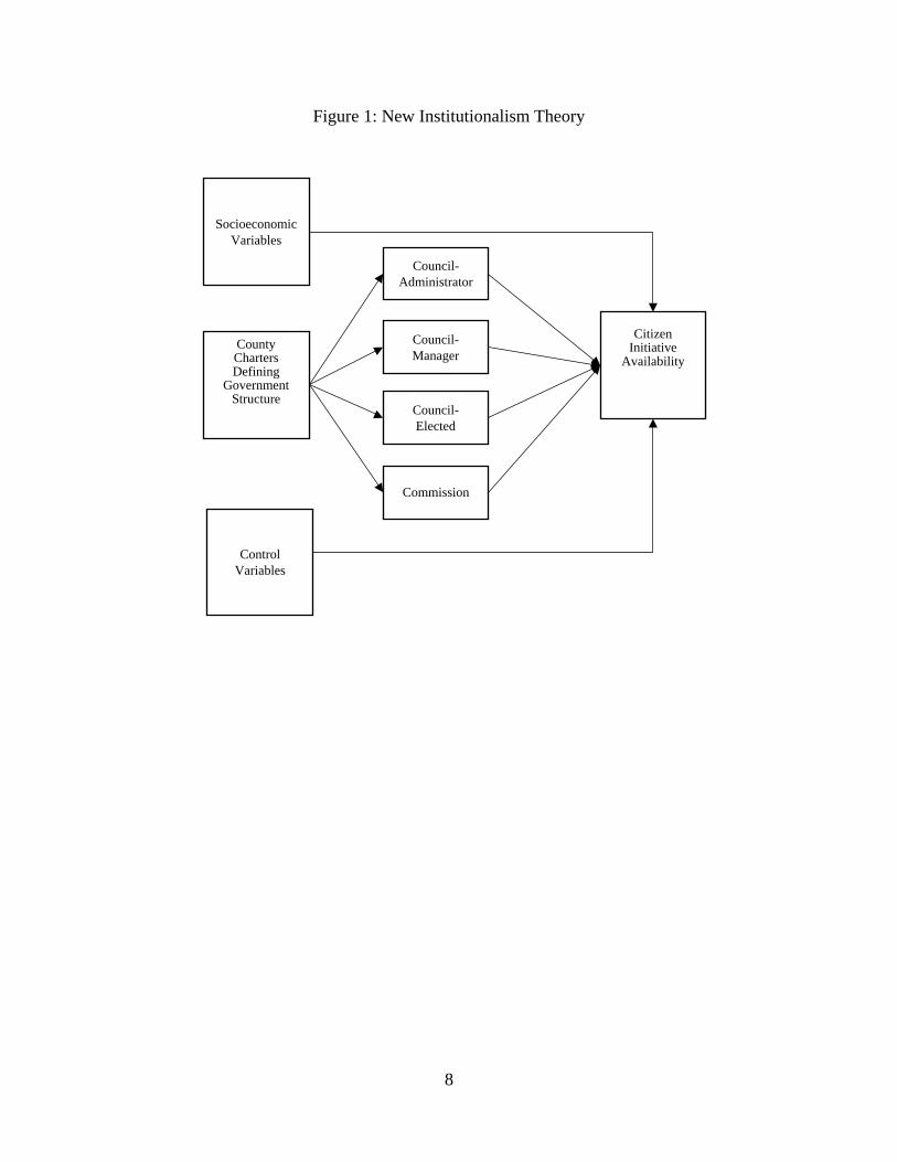
Below is a diagram of county government structure, socioeconomic variables, control
variables, and public policy outputs in the form of citizen initiatives adapted from (DeSantis &
Renner, 1996). Similar to DeSantis et al., this dissertation seeks to address the missing link in
addressing how different forms of county governments respond to citizen demands. This
dissertation addresses this research question by investigating the availability of citizen initiatives
in American counties. Specifically, this study uses new institutionalism to examine the
characteristics of the primary independent variable, the county forms of government. Additional
independent variables that are of interest include socioeconomic and control variables.
8
Figure 1: New Institutionalism Theory
County Charters Defining
Government Structure
Citizen Initiative
Availability
Socioeconomic Variables
Control Variables
Commission
Council- Manager
Council-Elected
Council-Administrator

9
Participatory Democratic Theory
Participatory democratic theorists claim that citizens would benefit if they participate
more directly in decision-making (Morrell, 1999). Participatory democratic theory (PDT) has
supported most of the past research regarding the effects of direct legislation such as the ballot
initiative and referendums (Dyck & Seabrook, 2010). Participatory democratic theory states that
the mode of participation derives among citizens in the workplace, household, community
setting, and the like (Hilmer, 2010). As a result, citizens that participate in direct democracy
receive an “educative” benefit since they absorb information through media exposure that can
increase political participation, especially those that are less educated (Tolbert et al., 2009).
Hilmer notes that the combination of these efforts creates the “general will” of the community.
However, Cebulam (2008) and Matsusaka, (2005) put forth an alternative reality
explaining that there can be null effects of the initiative on voter participation. Paralleling the
rational voter model, the probability of voting is an increasing function of the expected gross
benefits (EGB) associated with voting, and a decreasing function of expected gross costs (EGC)
associated with voting (Cebulam, 2008). The framework above requires that the benefits to
voting always be greater than the cost to motivate voter turnout. But, as Cebulam points out,
there are situations when this is not the case. Specifically, information costs put a burden on
voters in the form of investing time and effort to study and understand each initiative adequately.
Therefore, this study sets out to sort out this claim as well as investigate the effects of the
initiative at the county and state level.
The direct participation of citizens in local communities and workplace settings provide a
pipeline for increasing democracy integrated into political parties, rather than allowing elites to
set the agenda. Political scientists have had a keen interest in participatory democratic theory
10
dating back to the civil rights movement, with a special interest in the Voting Rights Act of
1965. After a brief drop in interest, the role of PDT has once again captured the attention of
scholars due to the prevalence of direct democracy in modern day politics.
The state's responsibility is not to necessarily mandate voting as a requirement for
participating in democracy. Rather, as Stein (2004) notes, coercion is not the sole province of the
state, instead, the state must make it possible for individuals to realize their own common good
through unobtrusive regulations. Therefore, it is left to the individual to reap the benefits of
participating in democracy through voting on policy, legislators, and identity. Smith (2002)
shows that building on participatory democratic theory, citizens that heavily use initiatives show
an increased capacity over the long term to correctly answer factual questions about politics. In
essence, participation is the basis for a truly free and equal society, and in return provides
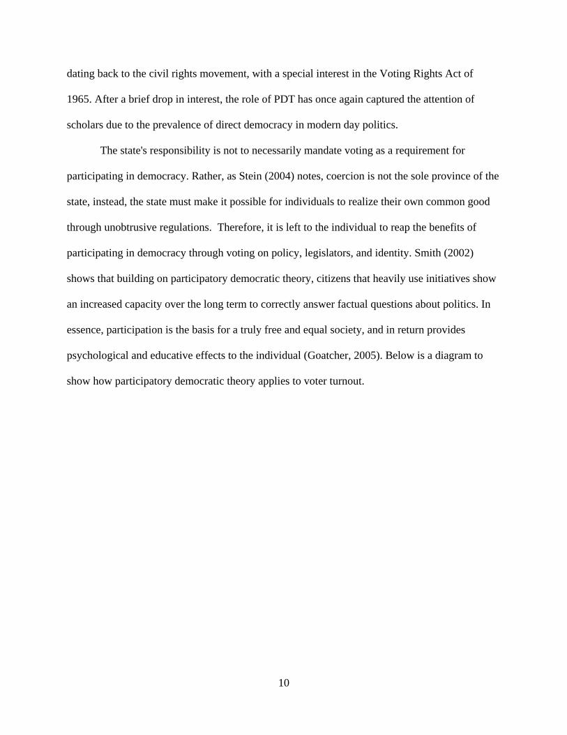
psychological and educative effects to the individual (Goatcher, 2005). Below is a diagram to
show how participatory democratic theory applies to voter turnout.

11
Figure 2: Participatory Democratic Theory
County Level Control
Variables
County-Level Voter Turnout
County-Level Citizen
Initiative Availability
County-Level Socioeconomic
VariablesLevel 1
Citizen Participation
State-Level VariablesLevel 2

12
Direct Democracy
Overview
This section will provide an overview and development of the citizen initiative in the
United States. The citizen initiative or “initiative” is a primary form of direct democracy, which
is a common reference due to its ability to initiate direct legislation by the voters. Goebel (2002)
defines the initiative as giving citizens the power to place a proposition on the ballot, with
enough signatures, and subject to popular vote.
During the early 1900s, the growth of the statewide initiative in the American west is
mostly explained by weaker political parties and stronger anti-monopoly sentiments (Goebel,
2002). According to one estimate, 726 constitutional and statutory initiatives were placed on the
ballots in the states with direct democracy between 1900 and 1939. During this time, the
progressive movement had a large focus on providing more political power to citizens. The
concerns about interest groups served as the underpinnings for many of the reforms during the
progressive era, to include moves toward direct democracy to rebalance the power in favor of
citizens (Grossmann, 2012). This era marked the creation of the citizen initiative or simply
“initiative,” which is a form of a direct democracy mechanism. President Woodrow Wilson
regarded the initiative as a mechanism to provide civic education to the electorate in the states
(Goebel, 2002). In this context, only a united people using instruments of direct democracy could
gain popular control of governments (Zimmerman, 2015). Advocates of the initiative further
point out that elected officials are little more than delegates to legislative assemblies with
detailed instructions on how to vote on bills (Zimmerman, 2015). Consequently, armed with the
initiative, the electorate does not need restrictive constitutional and charter provisions to protect
the public’s interest (Zimmerman, 2015).

13
One of the most active direct democracy states in the union is California. In fact, early
California politics revolved around anti-monopoly sentiments to protect railroad unions and the
like, which dates back to the early 1870s (Goebel, 2002). In 1912, the initiative became available
in Oregon. During the following years, observers pointed out that this direct democracy
mechanism liberated the state from the dominance of corporations, led to the passage of a series
of progressive laws, most notably the direct primary, and uplifted public morality in the state
(Goebel, 2002). Since then, there has been a steady increase in direct legislation after World War
II, with a noticeable uptick after the 1970s (Goebel, 2002).
The initiative performs an important civic educational function since a long-term
initiative campaign can have an educational effect on the legislative process (Zimmerman, 2015).
The initiative is based on the collection of a sufficient number of signatures on petitions directed
at state or county legislative bodies (Goebel, 2002). During tumultuous times in American
politics, the initiative can provide an avenue for citizens to bypass gridlock legislatures or inept
legislators. For example, in California, during economic swings in the 1990s, there were at least
50 percent more citizen initiatives on the ballot during this decade than any previous decade
since its introduction in 1911. The initiative allows voters to place proposed constitutional
amendments/statutes on the state ballot and propose charters, charter amendments, and ordinance
on the county ballot (Zimmerman, 2015).
The citizen initiative (initiative) may be direct, indirect, or advisory. Bowler, Nicholson,
& Segura (2006) concluded that political party organizations are rarely central players in citizen
initiative campaigns (Zimmerman, 2015). The direct initiative is when the entire initiative is
placed on the ballot if the requisite number and distribution of all signatures are collected and
certified; the indirect initiative appears on the ballot if the legislator fails to approve it first; and
14
an advisory initiative allows voters to circulate nonbinding questions on the ballot as a
mechanism to employ pressure on legislators (Zimmerman, 2015). For example, voters in 1983
approved proposition 9, a direct initiative, directing the mayor and the board of supervisors of
the city and county of San Francisco to provide ballots, voter pamphlets, and other materials on
voting in Chinese, Spanish, and English (Zimmerman, 2015). As of 2015, the initiative is
authorized by state constitutional and/or statutory provisions bearing in terms of authorized types
of initiatives, restrictions on use, petition signature requirements, ballot title preparation, a
system of verifying signatures, voter information pamphlets, and approval requirements
(Zimmerman, 2015).
In the American states, voters have decided on more than 600 statewide ballot
propositions in the 21st century (Matsusaka, 2014). No two states have the same requirements
for qualifying initiatives to be placed on the ballot (NCSL, 2012). Between 2000 and 2012, the
subject matter of popular initiatives in the United States consisted of health insurance (16.8
percent), education (9.8 percent), drug and alcohol matters (7 percent), electoral rules (5.7
percent), and civil constitution matters (5 percent) (Todd, 2014).
Citizens that choose to initiate ballots pursue this avenue for two basic reasons: 1) citizen
initiatives allow voters to directly constrain the actions of elected officials by enacting policies
they prefer, and 2) voters can propose initiatives in response to unpopular legislation (Phillips,
2008). Political science theorists contend that if democratic institutions offer people greater
opportunities to participate in decisions, those institutions may have an “educative” effect on
them (Smith & Tolbert, 204). As Milita (2015) points out, states have passed numerous laws
during the 2000s that make it more difficult for citizen initiatives to get on the ballot, e.g.,
increasing the number of signatures. Subsequently, more difficult requirements to qualify citizen
15
initiatives can be detrimental to public policy since citizens will have fewer opportunities to
bypass the inept legislator.
Benefits of Citizen Initiatives
In the early 1900s, governments often sought to spur economic development by granting
public powers to private individuals, such as giving away stretches of public land, granting the
right of eminent domain, or granting corporate charters (Goebel, 2002). For example, special
interest acquired political power and induced the state to grant them special charters, which then
allowed them to exploit and tax the public (Goebel, 2002). Subsequently, at the turn-of-the-
century, citizen initiatives gave populist new avenues to initiate legislation to check corporate
monopolies. Civic reform groups looked toward citizen initiatives to fight against corporate
trusts and monopolies oppressing farmers. The initiative formed as a direct democracy
mechanism by many different political fractions dissatisfied with American politics (Goebel,
2002). This simple mechanism holds the potential to affect both society and the economy
positively.
Bowler, Nicholson, & Segura (2006) demonstrate that the subject matter of a proposition
may be a national issue, a regional issue, a state issue, or a county issue. For example, a 1994
proposition sponsored by the Phillip Morris company wanted to remove control of smoking by
county governments (Zimmerman, 2015). In other words, the Phillip Morris company wanted to
maintain a free-wielding smoking policy that a county government wanted to regulate. In 1990,
the Southern Pacific Railroad initiated a rail bond measure, which included construction that
would aid the company in its development efforts. In both cases, the voters rejected the initiative
propositions (Zimmerman, 2015). These examples imply that even when special interest groups
or corporations sponsor initiatives, voters recognize the underlying motivations that may — in
these cases — go against the interest of the citizenry at-large.

16
A specific case of the initiative has been employed in 21 states to limit the number of
terms a member of Congress from each of the states may serve (Zimmerman, 2015). The idea is
that citizens can ensure a representative democracy of citizen legislators as opposed to
professional legislators representing only special interest groups. Many citizens view the
initiative as an antitax weapon, yet California proposition 10 of 1998 raised the state excise tax
on a package of cigarettes by fifty cents to eighty-seven cents (Zimmerman, 2015). But even in
this case, one can argue that this is simply an economic argument where the state wants to tax
bad behavior, and, preferably encourage good behavior (Thaler, 2015).
There is an abundance of academic literature showing that citizens become more
educated in the policymaking process when exposed to initiative campaigns (Tolbert et al.,
2009). High and frequent exposure to ballot measures has been shown to increase the awareness,
efficacy, political participation, and even the general level of happiness among citizens (Dyck,
2009). In 1979, U.S. Senator Mark Hatfield of Oregon was convinced that “the initiative is an
actualization of the citizen’s First Amendment right to the government redress of grievances”
(Zimmerman, 2015). Subsequently, the initiative can be a substantial check on the concentration
of political power.
17
County vs. State Citizen Initiatives
The citizen initiative operates differently between the county and state levels. The first
part of the dissertation focuses on the link between county governments and direct democracy at
the county-level. The second part of the dissertation focuses on the use of the citizen initiative at
both the state and county levels. First, I will describe the setting for which states permit citizen
initiatives at the county-level. The initiative at the county-level is regarded as localized
lawmaking, not centralized: each county asserts its right to self-government-granted by the
powers of home rule (Goebel, 2002).
State constitutions are the legal authority in granting home rule. (Benton, 2002). Park et
al. (2010) note that Dillon’s rule holds that county governments are “creatures of the state” and
can only undertake activities that the state specifically authorizes. However, nearly all states
have made provisions for municipal home rule allowing counties to enact charters that establish
rules of governance. Therefore, county charters provide options for county government, but the
selection of governance institutions is primarily a local choice (Park et al., 2010). Provisions for
a citizen initiative is an example of a local constitutional rule (Park et al., 2010). Consequently,
all states except for Wyoming and Indiana allow some form of the initiative at the county level,
i.e., 48 states (Graves, 2012; Todd, 2014).
The second part of this dissertation builds on the storyline of the first part by examining
the state-wide citizen initiative and the county-wide initiative in the 2016 presidential election.
Specifically, the second part analyzes the use of the statewide initiative in combination with the
availability of the countywide citizen initiative. At the state-level, direct democracy has
overwhelmingly been a phenomenon of the American West given that most of the states west of
the Mississippi river have adopted the mechanism (Goebel, 2002).

18
Consequently, 24 states allow the citizen initiative at the state-level (Tolbert et al., 2009).
These states allow citizens to place both a constitutional amendment and a state statute on the
ballot subject to a popular vote (Goebel, 2002). To summarize, after accounting for available
data, the first part examines county citizen initiatives available in 46 out of 48 states, while the
second part examines the citizen initiative in 23 out of 24 states. This research design reduces
endogeneity issues that may arise by isolating the models to states that permit either the county
or state level citizen initiatives while including appropriate control variables for each model
(Tolbert et al., 2009). Namely, in this dissertation, part one addresses the government structure
model, whereas part two addresses the voter turnout model.
Part I: The Link Between County Governments and Direct Democracy
County Citizen Initiatives
The dependent variable for part I is examining what factors contribute to the existence of
citizen initiatives at the county-level. The following section describes the application of the
citizen initiative at the county-level. For example, in 1986, Napa County, California voters
endorsed an initiative proposition that sought to preserve agricultural land and allow
amendments only by the voters (Zimmerman, 2015). Opponents of the proposition stated that it
frustrates the purpose of state planning law since accounting legislative body is powerless to
amend or repeal the initiative. Nonetheless, the California Supreme Court rejected this argument
and upheld the use of the initiative because it is the constitutional right of the voters to employ
the initiative (Zimmerman, 2015).
In 1998, voters in county governments approved close to 200 propositions regarding
growth control ordinances (Zimmerman, 2015). For example, in Ventura County, California,
voters approved a proposition removing the board of supervisors the authority to approve new

19
subdivisions and making each proposed subdivision subject to a referendum (Zimmerman,
2015). New York City voters in 1993 approved (60 percent to 40 percent) an initiative
proposition limiting city elected officers to two terms or a total of 8 years (Zimmerman, 2015).
In another case, a conservative group in Houston, Texas gathered 20,000 petition signatures to
place a proposition on a November 4, 1997 ballot stipulating that the city shall not discriminate
or provide preferential treatment of an individual based on race, sex, color, ethnicity, or national
origin (Zimmerman, 2015).
In each of these examples, the citizen initiative at the county-level allowed the local
citizenry to protect the environment, enact economic development measures, and ensure a
representative government, to name a few. Due to the evidence in the literature, the county
citizen initiative is just as valuable as the state level citizen initiative. The next section describes
various county governance structures that can influence the institution of citizen initiatives.
County Government Overview
As former U.S. House Speaker Tip O’Neil liked to say, “All politics is local” (Klinger,
2007). There is a common misconception about the development and structural dynamics of
county governments in the United States. This section will clarify any misconceptions and
review the major forms of county government to include their structure, constitutional
authorities, and leadership differences.
Moreover, this section sorts out the following research questions regarding government
structure in part one, which are the primary independent variables of interest. Are traditional
commission governments for politically sensitive to citizen issues relative to reform
governments? Are citizen initiatives more widely available in commission governments relative
to reformed governments? Are there structural differences between only reformed governments

20
that suggest a different response to enacting citizen initiatives? In the following section, I address
each of these questions in terms of examining the availability of citizen initiatives as the
dependent variable.
First, it will be helpful to review the development of county governments in the U.S.,
which have undergone tremendous change during the last century (DeSantis, 2007). After World
War I, three trends transformed the role of county government in the United States: (1)
population growth, (2) suburbanization, and (3) the reform movement to modernize government
structures (R. Campbell, 2007). Since the 1960s, counties have taken on more urban
responsibilities in order to respond to population growth such as providing political reforms,
public housing, and social programs (R. Campbell, 2007). As of this writing, there are 3,042
county governments in the United States; 48 states include areas of functional county
governments (Alaska has boroughs and Louisiana has parishes); (Salant, 2007). Three-fourths of
counties in the United States have populations of at least 50,000. The number of counties per
state ranges from 3 in Delaware to 254 in Texas; 8 states have fewer than 20 counties, and 7 have
100 or more, with an average of 64 for the U.S (Salant, 2007). Los Angeles County, California,
has more than 8 million residents, which is larger than the individual populations of 42 states
(Klinger, 2007).
County populations range from as low as 161 loving County, Texas, to 8 million in Los
Angeles County; the average is between 10,000 to 25,000 residents (Salant, 2007). County
government jurisdictions extend to more than 318 million residents in the United States (Pink-
Harper, 2016). This population growth has created new demands from citizens to improve
political processes.

21
Benton (2002) points out some scholars have argued that reformed governments produce
better public services, lower tax rates and expenditures, and more professional administration
while others argue the opposite. Regardless of reformed or traditional governments, counties
provide important services that promote economic development, enhance human capital, and
serve social safety net functions (Lobao & Kraybill, 2005). Counties also implement a growing
number of federally or state-mandated functions including health, welfare, law enforcement, and
education services (Menzel & Thomas, 1996). In addition to the increased demands on county
governments to provide services to residents in unincorporated areas, counties still need to
provide routine systems-maintenance functions such as voter registration, tax collection, and a
depository for vital statistics (DeSantis & Renner, 1996).
To review, a central research question in this study examines the impact of government
structure on the likelihood of providing the citizen initiative. For elected executives, the political
incentives of enhancing their chances for reelection are what drive them to find creative ways to
respond to median voter preferences. For appointed officials, professional incentives intertwined
with the desire to improve their careers are what drive them to become strategic planners and be
innovative in addressing county deficiencies (Farmer, 2017). Since citizens find the initiative a
useful direct democracy mechanism, it will be more likely to exist with the county governments
that incorporate the greatest stipulation for elected officials. This study argues that the citizen
initiative will be most prevalent in counties that have the commission/council-elected
governments relative to the council-manager/administrator governments. The following sections
will delve into this rationale more comprehensively.
Empirical research has largely focused on the effects of the progressive era on reforming
county governments. The reform efforts aimed at U.S. counties focus on professionalizing

22
operations and providing expansions and services, and an alternative form to the traditional
commission form of government (Deslatte, 2017; Pink-Harper, 2016). These reformed
government structures stipulate that a county executive serves alongside the traditional
commission government to handle responsibilities that range from fiscal to political duties. The
reformed governments include the council-elected, council-manager, and council-administrator
governments. Conversely, the classical, commission form of government allows a board of
commissioners to hold executive and legislative authority by which a board of commissioners
divides administrative functions and duties between commissioners (Deslatte, 2017).
Academic research has largely focused on federal, state, and municipal governments with
little attention focusing on county governments (Salant, 2007). Discussion of American counties
typically generates diverse views on the usefulness and role of county government that ranges
from praise to judgments of obsolescence in the 21st century (Salant, 2007). The two primary
functions of counties are to (1) govern, and (2) deliver services (R. Campbell, 2007). Since a
county is a product of the state, the academic literature refers to it as a local government, like a
city. Nonetheless, as Benton (1996) notes, the academic literature has given little consideration
that findings for cities and counties might differ when analyzing local governments.
The form of government is an important variable to consider when investigating public
policy outcomes at the local-level. Most counties must cope with providing rapidly escalating
demands for urban-type services, the continued evolution of federal domestic policy
responsibilities, and the growing interdependencies of city, county, regional, and national
economies (Streib, 1996). Conflict and cooperation in and among American counties are
important but neglected subjects of scholarly study (Klase, Jin, & Gerald, 1996). Klase et al.
explains that conflict can arise between or among individuals based on social and political

23
structure rather than marginal differences in styles, personalities, or methods of work (Coser,
1956).
In this context, social and political structures are inherent in the different forms of county
governments. Specifically, county officials are the primary actors who define agenda setting,
policy formulation, and program implementation (Klase et al., 1996). Consequently, the conflict
among county officials can be drawn out due to regulations across different intergovernmental
bodies (Daniels, Walker, & Emborg, 2014). Namely, the modernization movement that has
transformed many counties from narrowly focused arms of the state to entities resembling full-
service municipalities has been accompanied by stress, strain, and conflict (Klase & Song, 2000).
The governing boards of U.S. counties approve government programs and activities that
surpass billions of dollars annually (MacManus, 1996). Such governing boards range in size and
scope depending on the form of government. Board representativeness includes factors that
pertain to partisanship, gender, race, and age composition, whereas board openness concerns
vacant seats, the incumbency return rate, and trends in the electoral competition (MacManus,
1996). Moreover, as MacManus notes, many counties experienced a change in electoral systems,
which can be prompted by the initiative.
The size of governing boards typically ranges between three and seven members, with a
few exceptions due to some Voting Rights Act cases, i.e., Michigan counties can have up to a
staggering 35-member board. In these instances, the federal courts ordered jurisdictions to
increase the size of their governing bodies to be more representative of majority – minority
districts (MacManus, 1996). Board members typically have a two-term limit with each term
lasting between two and four years; however, there is no evidence of a relationship between the
length of term and form of government (MacManus, 1996). Moreover, most county governments

24
hold elections in even years, typically the same year’s elections are held for the president
(MacManus, 1996). Electoral system changes at the county-level have been the direct result of
citizen initiatives and legislative referendums (MacManus, 1996). Many of these changes focus
on board size, term limits, partisan ballots, filing fees, and petition signature requirements.
Tekniepe & Stream (2010) note 1) county governments provide citizens their best
opportunity to obtain a response from government, 2) counties provide a means of citizen access
to the policymaking process at the level with which they have the easiest access, and 3) counties
are perceived to be the most responsible for service delivery. A contemporary view recognizes
that counties are a major provider of local services as well as an arm of the state, where they
must meet citizen demands both within and outside of municipal boundaries (Salant, 2007). For
example, in Pennsylvania, the county became the primary unit of local government because of
the states widely dispersed population, and county governing bodies, called boards of
commissioners were elected at-large (Salant, 2007). Therefore, the county took on dual
responsibilities by acting as the administrative arm of the state and as a local government (Salant,
2007). However, rather than simply acting as the administrative arm of the state, the county has a
whole host of responsibilities to provide to its citizens that have increased in the recent decades.
The administrative arm of the state means that the county must provide indigent services
under state mandates, which can include medical and institutional facilities for individuals who
do not qualify for federal, state, or community programs. Additional responsibilities can include
tasks carried out by officers such as an assessor and treasurer in unincorporated areas, and
providing services to the county hospital, the county superior court, and road construction and
maintenance (Salant, 2007). Subsequently, county officials must grapple with affordable

25
housing, clean air, water quality, AIDS prevention and care, refugee settlement, criminal justice,
transportation, and managing natural disasters (Salant, 2007).
Commission Governments
The traditional commission government has been in operation for most of the 330-year
history of counties in the United states, whereas the reform movement started to take place after
World War I (H. Duncombe, 2007). By 1975, 40 states permitted at least one alternative to the
commission government, which includes the reformed governments that attempt to separate the
powers of the executive and the commission (H. Duncombe, 2007; Pink-Harper, 2016). This
section will focus on the development of the commission government, whereas the next section
will review the reformed governments.
This study argues that commission governments are the most democratic form of
government, and therefore, reflect the views and attitudes of the citizenry the greatest. Thus, as
public opinion polls show, the citizen initiative is mostly seen as a useful direct democracy
mechanism that helps citizens become active in the lawmaking process (Dalton, Bürklin, &
Drummond, 2001). If these arguments provide insight into the availability of the citizen initiative
at the county-level, then it will be prevalent in commission governments.
In the American West, during the early 1900s county governments began to experiment
with commission governments while implementing direct democracy mechanisms (Goebel,
2002). Since then, traditionalist cultures have been reluctant to abandon the commission form of
government (DeSantis & Renner, 1996). Thereafter, these developments led to a wide variation
of county governments that permit the citizen initiative. In the commission structure, voters
separately elect a legislative body – usually called the board of county commissioners – that have
limited policymaking power and many executive department heads (DeSantis & Renner, 1996).

26
Furthermore, voters separately elect a legislative body that has limited policymaking power, and
a large number of executive department had such as the county clerk, tax assessor, tax collector,
sheriff, and supervisor of elections, to name a few (DeSantis & Renner, 1996).
Some scholars have gone as far as to refer to the commission government as a conflict
model (R. Campbell, 2007). President Woodrow Wilson, in an essay entitled “democracy and
efficiency,” claim that democracies are intrinsically inefficient, suggesting that the least
democratic is more efficient (R. Campbell, 2007). However, the trade-off for efficiency is more
democratic systems that respond to citizenry values and interests aptly.
Menzel & Thomas (1996) point out that most county officials are elected and want to
retain or seek higher public office, they may have little choice but to respond to the service
demands of residents. Menzel et al. continue, it may well be that a counties response to citizens
is stimulated by electoral competition, which has validity at the state government-level.
Consequently, this same validity is certainly possible at the county-level when factoring in the
partisan elections that concern county commission governments.
As Benton (2007) points out, little is known about citizen participation in county politics
compared to participation in elections for national or state-level offices. Therefore, it is up to
policymakers and citizens to approve county charters at the local-level to decide whether to
allow a citizen initiative on a case-by-case basis. Unlike cities, counties include incorporated and
unincorporated jurisdictions (Pammer, 1996). Nonetheless, counties are responsible for
providing services to both jurisdictions.
In the commission form of government, county administration is frequently divided
among competing branches, fractions, or personalities and therefore is not centrally controlled
(MacManus, 1996). The more highly politicized the government structure, as in traditional,

27
unreformed locales, the more likely it is the conflict arise (Klase et al., 1996). In reformed
governments, interactions among officials and counties are less politicized and characterized by
cooperation due to the presence of essential authority figures such as the council-manager or
council-elected representative (Klase et al., 1996). However, in the case of enacting the citizen
initiative at the county level, the role of partisanship is indispensable.
White & Ypi (2011) summarizes favorable commission government arguments with the
following: 1) the role of partisanship is probed and affirmed since it invites debate, 2) the
constituency that offers such political justifications, 3) the circumstances in which the
development of the political justifications occur, 4) the ways in which they are made inclusive,
and 5) the ways in which they are made persuasive. Thus, debate and conflict, more prevalent in
the commission form of government would suggest a higher likelihood for direct democracy to
exist. These advantages of the commission government are in sharp contrast to the reformed
governments except for the council-elected government, which has a central figure with fewer
political constituents to serve.
A common criticism of the commission government is that the absence of a chief
executive provides no effective supervision or coordination of department heads and
policymaking (H. Duncombe, 2007). However, as Farnham (1987) points out, based on the
median voter theorem, elected officials in the commission government respond to citizen
demands more than reformed governments. In fact, the more politicized nature of commission
governments prompts county commissioners to spend in response to political demands (Choi et
al., 2010). Rather, under the commission form, elected officials are expected to act in accordance
to the desires of their constituents by remaining responsive to their citizens and acting to protect
themselves from future electoral threats (Pink-Harper, 2016; Tekniepe & Stream, 2010).

28
Typically, the commission government consists of three to five members elected from at large or
single-member districts (Pink-Harper, 2016). Subsequently, this governing body possesses both
legislative and executive authority (Pink-Harper, 2016).
Smaller counties are more likely to maintain the commission form of government since
they are less likely to be granted home rule status by the states (MacManus, 1996). The lack of
home rule status for a commission government may inhibit smaller counties to enact the citizen
initiative. However, the research design for this study accounts for this issue by incorporating
home rule as an independent variable.
The commission form of government accounts for 77 percent of all counties but governs
only about 49 percent of people in the United States (H. Duncombe, 2007). The commission
government requires that each elected commissioner serves as the director of one or more
functional departments in addition to making policy; under the council-manager form, “an
elected board sets policy, adopts legislation, and the budget”; and finally, the council-elected
government requires that commissioners make policy whereas the executive elected prepares the
budget (MacManus, 1996). The county clerk in commission governments often serves as
secretary to the county board, which may include recording the actions of the board, registering
voters, and publishing election notices (H. Duncombe, 2007). The most contentious elections for
county commissioners involve the partisan ballot, which most large counties have retained since
the 1990s (MacManus, 1996). In this case, the county commissioner running for office is listed
on the ballot with an indication of their political party.
An elected county commission has both legislative and executive responsibilities. The
legislative authority includes enacting ordinances, levying certain taxes, and adopting budgets;
whereas the executive authority includes administering local, state, and federal policies,
29
appointing county employees, and supervising transportation projects (Salant, 2007). The
commissioners are usually elected by district within the county (DeSantis, 2007). Administrative
responsibilities are also vested constitutional offices, such as a county sheriff, treasurer, coroner,
clerk, auditor, assessor, and prosecutor (Salant, 2007). A study completed in 1975 reported that a
civil rights group was more successful in having their demands met in commission cities rather
than reformed cities (Menzel, 2007). Feiock (2004) shows that county government policy is
driven primarily by political incentives of local actors as preferences of the median voter.
Consequently, county commissioners that make up unreformed governments respond to political
demands, particularly from organized advocates in the community (Choi et al., 2010).
There are advantages of the commission government. The traditional commission
government has longevity since it is the traditional structure of county governments in the United
States (H. Duncombe, 2007). The commission plan brings government administration close to
the people through the independent election of government department heads; therefore, it is the
most democratic form of government (H. Duncombe, 2007). This form of government mimics
the legislative bodies at the state and national levels, which has its roots in the U.S. Constitution.
The commission government has a broadened system of checks that is provided by the
individual elections of each official, which lessens the chance of a corrupt government (H.
Duncombe, 2007). The commission government has a unified process to make policy since the
board administers both legislative and executive functions. However, this last point is debatable
since it depends on whether the county officials are of the same party and follow agreements
worked out with party leaders (H. Duncombe, 2007).
Duncombe (2007) notes several variations of the commission government that offers
some clarification on misconceptions that may exist in the literature. In some counties, the chair
30
of the board may have greater seniority, greater ability, more experience, and make most of the
administrative decisions leaving the other commissioners to share in the legislative and policy
making actions (H. Duncombe, 2007). In other counties, there is an appointed county clerk who
aids the county commissioners in preparing the budget, developing agendas or board meetings,
following up on board decisions, and advising the commissioners on emergencies that would
wear their attention (H. Duncombe, 2007). These variations on the commission form suggest the
added efficiency of the reformed governments, but, yet maintains the democratic norms of a
commission government that most closely reflects the attitudes of the citizenry.
As described above, Duncombe (2007) points out that many counties have a chair of the
board that helps unify administration by assuming a strong leadership role. Granted, this would
lend support for the case that the county should transform to a reformed government, but until it
does so, it will carry the classification as a commission government. The arguments in this
section support the notion that the citizen initiative will be more likely to exist with the
commission form of government. Similar to the commission government, the council-elected
government is a type of reformed government where the executive is elected by an election at-
large. Subsequently, the chief argument in the government structure model is that the citizen
initiative will be more likely to exist for both the commission and council elected governments. I
discuss this in greater detail in the next section.
Reformed Governments
The premise of the reformed models is that administrative services should be handled
separately by the executive (Benton, 2003; Pink-Harper, 2016). As such, executive leadership
matters for reformed government structures. As noted by Carpenter, Geletkancz, & Sanders
(2004), organizations are typically a reflection of top management. The reformed government

31
structure includes an executive with special powers that can make policymaking decisions with
long-term implications. Additionally, the executive is responsible for agenda setting, preparing
budgets, and making department head appointments (Tekniepe & Stream, 2010). However,
there are trade-offs for the advantages of the reformed model.
According to Bridges, reformed governments create barriers to political voting and
participation, and insulate politicians and government from the demands of lower-income and
ethnic groups (Wood, 2002). Although reformed governments promised efficient administration,
sustained economic growth, low property taxes, honest government, and adequate public
services, often lower-income neighborhoods and groups were excluded from these benefits
(Bridges 1997a; Wood, 2002).
County reformers have made substantial efforts to change government structure by
urging shifts from the traditional county commission to a central executive authority (i.e., either
appointed or elected) (DeSantis & Renner, 1996). Therefore, reformers advocate switching to a
version of the county executive form. But has there been any limitations on direct democracy
mechanisms for counties that have decided to switch to reformed governments? Specifically, is
the citizen initiative less available in reformed governments? This section will sort out these
questions, and argue that of the reformed governments, the council-elected government is most
conducive to providing the citizen initiative.
There are three basic types of reformed county governments: 1) council-elected, 2)
council-manager, and 3) council-administrator. As of a 2007 study, there were roughly 786
counties that have the council-manager or council-administrator government, and 383 counties
that have the council elected form of government (Salant, 2007). The reformed governments also
have a governing board that consists of independently elected officials; however, these
32
governments tend to have fewer governing board members with diminished powers (H.
Duncombe, 2007). Reformed governments are often indicative of lower political responsiveness
and lower taxing and spending, perhaps because decision makers are more insulated from
potential conflicts and professional managers have more power in reformed governments
(Menzel & Thomas, 1996). This study extends this argument with one caveat; the council-
elected has an elected executive who can respond to political considerations that best reflect the
attitudes and interest of the citizenry.
In terms of leadership, the county executive must be a strong coalition advocate. (Svara,
1996). There are several examples of a strong county executive implementing policy. In 1982,
Parris Glendening, elected as a county executive in Maryland engineered a renaissance of the
county by improving the fiscal condition, business limit, environmental programs, and the
educational system (Svara, 1996). In 1986, Edward McNamara, elected as county executive in
Wayne County, Michigan reorganized county government, made management changes,
improved control for health and childcare cost for indigents, and fostered economic development
initiatives (Svara, 1996). In fact, Lewis (1993) found a high correlation between productive
county managers and environments where the public is more accepting of government action.
Moreover, county managers can act as a neutral third-party to mitigate partisan electorates where
commissioners must battle during election time. Pammer (2000) notes that county managers
must manage partisan issues to foster cooperation in a fragmented government. Therefore,
reformed governments are considered to be proactive given the executive manager that has sway
over policymaking initiatives (Menzel, 1996).
Critics of the commission form of government note that three or five person boards
generally suffer from fragmentation of authority and the lack of a politically accountable chief
33
executive (Streib, 1996). Streib & Waugh (1991) found that council-elected governments have
higher spending levels than other reformed governments. These higher spending levels are
mainly attributable to supporting capital improvement projects based on citizen demands.
Therefore, this section argues that in addition to the commission government, the council-elected
government is conducive to making the initiative available to county citizens.
Council-Elected Government
The council-elected executive form features and independently elected executive who is
considered the formal head of the county (Pink-Harper, 2016). The council-elected executive is
independently elected by the people to perform specific executive functions for the executive
branch of government (Salant, 2007). The county board remains the legislative body, but the
county executive may veto ordinances enacted by the commission (Salant, 2007). Conversely,
the commission board usually has the power to override the county executive with a two-thirds
or greater majority (H. Duncombe, 2007).
The elected executive plan is in place in counties ranging in population from 77,000
(Putnum County, New York) to 1.3 million (Nassau County, New York) (Menzel, 2007). This
plan is popular in New York because each county has the considerable legal flexibility to tailor
the plan to fit local needs and conditions (Menzel, 2007). Moreover, the elected executive
occupies a highly visible political role in New York, one which is has been a stepladder for
several officials into higher office. For example, in 1977, Erie County’s elected executive,
Edward Regan was later elected to state comptroller; and in 1982, Alfred DelBellow who served
as an elected executive in Westchester County was later elected to lieutenant governor (Menzel,
2007). Additionally, in many states, elected executives run on partisan ballots. Such a stepladder

34
process can be beneficial for citizens to identify candidate expectations due to political party
affiliations (Mangum, 2013).
Schneider & Park (1989) note, “the data show that county governments with reformed
structures (especially elected county executives) spend more and provide more services than
counties with the traditional commission form of government” (Ybarra & Krebs, 2016). Thus, a
positive relationship exists between highly politicized forms of government, even if reform and
structure, and the level of spending and service provisions.
More populous counties tend to use the council-administrator or council-elected forms of
government (H. Duncombe, 2007). As Menzel (2007) notes, some citizens have asserted that
elected county executives must bring both strong political and administrative leadership. In 1977,
there were 142 counties with over 43 million residents, which employed the council-elected form
of government (H. Duncombe, 2007). The council-elected form is most similar to the strong
mayor system at the municipal level, where the commissioners are responsible for both
legislative and executive duties. Thus, it is not far-fetched to say that a county elected executive
is comparable to a governor, or even to the President of the United States, given the executive
functions that he or she carries out as an elected official (H. Duncombe, 2007).
Subsequently, this individual is the top elected party official at the county level (H.
Duncombe, 2007). The executive elected at-large implements county board policies and often
has veto power (Istrate & Mills, 2018). The movement toward independently elected executive
has made the title of county-executives much more prevalent (DeSantis, 2007). About 69 percent
of counties select the elected executive based on recommendations from commissioners, while
22 percent of counties opt to elect the executive based on citizen votes (DeSantis, 2007). In
either circumstance, the executive derives his or her position based on an election process.
35
Berman (1993) examines the policy decisions made by four county commissions in
Illinois and California. Berman finds that county commissioners in Illinois spent about 80
percent of the total meeting time on administrative matters as opposed to policy decisions. The
findings for the California counties are similar, where commissioners spent about 65 percent of
the total meeting time on administrative matters (Berman, 1993).
This section provides a rationale that county commissioners are modestly involved in
policymaking to fulfill the responsibilities of the governing board. In this case, these findings
suggest that executives play a larger role in the policymaking process. Consequently, it is the
county executive that appears to have some part in spearheading legislation to meet citizen
demands.
The elected executive provides the needed strong political leadership for relating to
diverse segments of the community and is less likely to resign during a crisis of change (H.
Duncombe, 2007). Moreover, the elected-executive must answer to both government officials
and the county electorate in the next election, and therefore state legislators, governors,
congressional members, and the president can focus on one elected executive that represents the
county (H. Duncombe, 2007). Therefore, along with the commission government, this section
argues that the council-elected government is also conducive to providing the initiative to
citizens.
Council-Manager Government
The council-manager form of government has a legislative body, which appoints a county
manager who performs executive functions, such as appointing department heads, hiring county
staff, administering county programs, drafting budgets, and proposing ordinances (Salant, 2007).
Under the council-manager form, the appointed administrator possesses power equal to those in
36
the city manager by setting the legislative agenda, controlling the budget, appointing department
heads, and overseeing general county operations (Benton, 2002). The council-manager has the
most extensive powers of the three types of reform governments. Council-manager governments
vary in size from Dade County (Florida) with a population of more than 1.2 million, to petroleum
County (Montana), with a population of less than one thousand.
Political partisanship and the form of government have been central issues in the debate
about county leadership. As Nalbandian (1990) points out, the council-manager government was
borne out of the reform movement at the turn-of-the-century with an explicit goal of reducing
corruption and improving efficiency. The chair of council-manager governments has a set of
responsibilities that separates it from other forms of government. Namely, Svara (1996) explains
that the county commission chairs that have a manager accomplish objectives by setting goals,
identifying problems, coalescing the council, educating the council, and developing a policy
agenda.
As noted, most county commissions are plural executive bodies (Svara, 1996). As such,
commissioners exercise executive functions not assigned to other elected official boards, or the
delegate functions to an appointed administrator (Svara, 1996). Most notably, the formal role of
the commission of the governing board for the county is its low involvement in legislative
activity (Svara, 1996). Ammons & Newell (1988) argues that county managers are similar to city
managers, and in practice, city managers are less insulated from politics and more active in
policy processes than the 19th century reformers had ever imagined. Thus, the county manager is
not necessarily concerned with the attitudes and interest that are of primary concern to the
electorate.

37
Council-Administrator Government
The council administrator government is similar to the council-manager form in that it
has a chief executive to supervise county departments. However, in this case, the chief executive
is also appointed, but with more limited capacities relative to the council-manager. Under the
council-administrator government, the commission does not appoint department heads to prepare
a budget, draw ordinances, and oversee program implementation (Salant, 2007). Rather, the
council-administrator plan separates policymaking and administration, thus removing the
administration from political influence.
The chief administrator government is most widely used in California and is the form
used in the nation’s most populous county, Los Angeles (H. Duncombe, 2007). Large urban
counties such as Montgomery County (Ohio) and Alameda County (California) are among the
many large urban counties was small county boards, which have delegated much of the
administration to the appointed administrators (H. Duncombe, 2007). Conversely, Michigan
counties can have between 5 and 35 commissioners on a board (H. Duncombe, 2007).
Duncombe (2007) notes that according to an ICMA survey of 202 counties, council-
administrators do not want to exercise political leadership. The lack of political leadership is
primarily because these administrators cannot become the political representative of the county
without destroying the employee – employer relationship and without destroying the basis for
electing the governing board (H. Duncombe, 2007). However, as previously discussed, political
considerations hold our representatives accountable. If a chief executive in power has no vested
interest in direct democracy, then he or she will do little to help provide this utility to the
citizenry.
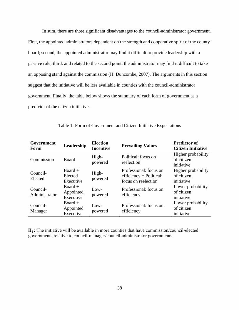
38
In sum, there are three significant disadvantages to the council-administrator government.
First, the appointed administrators dependent on the strength and cooperative spirit of the county
board; second, the appointed administrator may find it difficult to provide leadership with a
passive role; third, and related to the second point, the administrator may find it difficult to take
an opposing stand against the commission (H. Duncombe, 2007). The arguments in this section
suggest that the initiative will be less available in counties with the council-administrator
government. Finally, the table below shows the summary of each form of government as a
predictor of the citizen initiative.
Table 1: Form of Government and Citizen Initiative Expectations
Government Form Leadership Election
Incentive Prevailing Values Predictor of Citizen Initiative
Commission Board High-powered
Political: focus on reelection
Higher probability of citizen initiative
Council-Elected
Board + Elected Executive
High-powered
Professional: focus on efficiency + Political: focus on reelection
Higher probability of citizen initiative
Council-Administrator
Board + Appointed Executive
Low-powered
Professional: focus on efficiency
Lower probability of citizen initiative
Council-Manager
Board + Appointed Executive
Low-powered
Professional: focus on efficiency
Lower probability of citizen initiative
𝐇𝐇𝟏𝟏: The initiative will be available in more counties that have commission/council-elected governments relative to council-manager/council-administrator governments

39
Home Rule Charter
Since counties are a derivative of their state, I now turn to the importance of home rule.
Home rule refers to a state constitutional provision or legislative action that provides county
governments with greater measures of self-government (Bunch, 2014). As Klase et al. (1996)
notes, home rule can have a significant impact on the structural determinants of modernized
governments, and how each government meets citizen demands. In this section, I intend to
examine this question in the context of citizen initiatives.
Menzel & Thomas (1996) pose the following question: do counties with home rule status
act with greater authority relative to counties that are not? The primary argument behind home
rule is that the county government has a better understanding of local needs and tradition and is
better suited to handle the request of autonomy (DeSantis, 2007). Based on home rule, if county
circumstances warrant it, the state may allow the county to play an important role in establishing
the initiative (Thomas, 2007).
City charters structure the incentives of political actors and determine the kinds of
decisions that will be rewarded at the county level (Park et al., 2010). County charters function
similarly to influence policy decisions that will (or will not) be rewarded. These rewards,
afforded through the home rule charter, exist in wide variations throughout the United States
(Bunch, 2014). As Menzel et al. notes, county officials who are hit hardest by increased
population growth are more likely to be in the forefront of the effort for home rule and an
expanded role of counties. For any institutional arrangement, testing for the home rule effect can
isolate the effect of the government structure (Becker & Antic, 2016). Therefore, different formal
government structures are expected to lead to different policy outcomes (Park et al., 2010).
40
The difference in policy outcomes due to government structures will be an important
proposition to test since there is a wide variation in American counties that have decided to pass
the citizen initiative at the county-level. Given that counties can be essential in the allocation of
regional goods, such as land use, development, and public transit, one must consider the
importance and implications of their institutional settings on policy choices (Farmer, 2017).
Dillon’s rule holds that county governments are “creatures of the state” and can only undertake
activities the state specifically authorizes (Park et al., 2010). Conversely, home rule delegates
structural (the power to choose form a government) and functional (power to exercise local self-
government in a broad or limited manner) authority to county governments (Benton, 2003).
Menzel & Thomas (1996) notes, the more recent the state constitution, the more discretion given
to county governments in the form of home rule.
I will now describe the application of home rule as it relates to county government
autonomy. Save Palisade Fruitlands, a citizens group brought a section 1983 action against the
County Clerk of Messe County, Colorado, and alleged that the clerk’s denial of the group’s
request to place an initiative land-use proposal on the ballot violated the equal protections rights
of voters in statutory counties (Zimmerman, 2015). Save Palisade argued that the provision
allowing only home rule counties to employ the initiative is subject to strict scrutiny under the
equal protection clause of the U.S. constitution (Zimmerman, 2015). Thereafter, the U.S. District
of Colorado concluded that there was no denial of equal protection, to which the group appealed
to the U.S. Court of Appeals in the tenth circuit (Zimmerman, 2015). The US Court of Appeals
agreed with the lower court but added that the appellants could lobby the state legislator to grant
the initiative power to statutory counties (Zimmerman, 2015). Thus, home rule stands as an

41
important state law that permits counties to permit the initiative; however, it is still the county
government charged with enacting the initiative as a local direct democracy mechanism.
Moreover, home rule gives counties the authority to have a position of appointed
manager or elected executive, and alter the method of electing commissioners and the size of the
board (DeSantis, 2007). Additionally, home rule allows counties to control their finances and
remote budgetary stability with regard to rules governing county debt and revenue (DeSantis,
2007). Choi et al. (2010) point out that the home rule option allows counties to provide better
services for citizen demands that include judicial services, welfare, and transportation.
Jurisdictions lacking powers of home rule are precluded by Dillon’s Rule from providing
services that go beyond the scope of those authorized by their states (Farmer, 2017). Such
jurisdictions lacking the home rule charter may have less to spend on expenditures for promoting
public policies (Choi et al., 2010; Farmer, 2017). Therefore, these increased services are likely
to fall in line with meeting citizen demands that can include providing the citizenry with the
initiative.
𝐇𝐇𝟐𝟐: The initiative will be available in more counties where states permit the home rule charter
Socioeconomic Variables
This section will describe socioeconomic factors as predictors of political processes for
instituting the initiative. The socioeconomic factors of interest are per capita income, persistent
poverty, and educational attainment. Each factor may have its contribution to the presence of an
initiative. The dissertation outlines the relevant literature below.
42
Per Capita Income
First, this study reviews income potential as a predictor of county government outcomes.
A fundamental concern for American democracy is that citizens’ political preferences are
weighed equally by their elected officials, and disadvantaged groups such as the poor are not
locked out from policy representation (Griffin & Flavin, 2011). Pacek & Radcliff (2008) explain
that investigating the impact of income inequality on policy outcomes is an ongoing debate in the
public administration literature. The initiative has a strong economic component since it allows
citizens to initiate legislation that removes powerful special interest groups, oppressive
monopolies, and corporations (Goebel, 2002). Klase et al. (1996) note that economic variables
such as per capita income can impact county outcomes.
In principle, per capita income reflects the wealth and revenue base of the general
environment and thus indicates the level of resources potentially available for facilitating outputs
(Klase et al., 1996). Pammer (1996) points out that both per capita income and poverty levels
substantially affected the services provided by the city of Dayton. Thus, wealthy citizens have a
greater opportunity to address these gaps in public policy than poorer citizens (Skocpol &
Jacobs, 2012). Moreover, Radcliff & Shufeldt (2016) find evidence that the citizen initiative has
the highest benefit for citizens with the lowest income. While Radcliff et al. show the initiative
helps the lowest income bracket, there is no evidence in the study regarding the influence of per
capita income on the availability of the initiative. Meanwhile, Bollen & Jackman (1985) found
no evidence of income inequality having an impact on political democracy, i.e., the number of
political parties available.
Flavin (2012) investigates the pivotal question of “Who does the government respond to
when formulating public policies?”. Flavin’s study reveals that citizens with low incomes receive

43
little substantive political representation compared to more affluent citizens in the policy
decisions made by the state government. This study is pivotal because it shows that an “unequal
democracy” exists, at least to some extent, in the United States (Flavin, 2012). Therefore, the
income potential for a county can very well contribute to public policy outcomes. Griffin &
Flavin (2011) show that citizens with higher incomes place a higher priority on policy
representation and less on constituency service then do those with lower incomes. This study
proposes that higher per capita income will provide greater resources for voters to enact citizen
initiatives.
𝐇𝐇𝟑𝟑: Counties with higher incomes per capita are more likely to have the initiative
Poverty is typically the result of low income. Thus, there is a high correlation between
both per capita income and poverty. However, this study uses a unique 30-year persistent poverty
measure to capture the long-run effects of a community in economic turmoil. Accordingly,
several examples show the effects of persistent poverty on public policy outcomes. As Lobao &
Kraybill (2005) note, nonmetropolitan counties are typically characterized by lower incomes and
higher poverty. Moreover, Lobao et al. point out that any reduction in county services impacts
higher poverty counties more severely.
Delabbio & Zeemering (2013) show that counties with high levels of poverty are more
proactive in reaching out to other local governments to construct interlocal agreements. Such
interlocal agreements means that county leaders play an active role in attempting to find new
political institutions to bolster economic development. Farmer (2017) finds that counties with
higher poverty rates, spend less on service spending. Therefore, it is conceivable that a county
with a high poverty rate would have fewer resources to support political change. In sum, the
44
literature suggests that higher poverty would lead to less spending by county governments and
fewer resources to support instituting the initiative.
𝐇𝐇𝟒𝟒: Counties with higher persistent poverty rates are less likely to have the initiative
The educational attainment of a county population can play a key role in establishing the
initiative since the commission board and executive often come from the county citizenry.
Moreover, the impetus for policy change at the county level is often the result of political
participation. This section outlines the literature relevant to examining the influences of an
educated population on instituting the initiative at the county-level.
Collingwood (2012) found that voters with a college degree are more likely to be
supportive of citizen initiatives. Bowler & Donovan (2002) find evidence of a positive
association between education and an individual’s political participation in citizen initiatives.
Burnett & Parry (2014) find insignificant evidence that education has a bearing on voting for
legislative referendums (a form of direct democracy) on a state ballot regarding the support of a
health initiative, and two bond measures regarding bond support for higher education (in 2006)
and roads (in 2011). As a result, the literature mostly suggests that counties with a highly
educated population (e.g., those that have a bachelor’s degree or higher), would be more likely to
engage in political participation. Therefore, this study tests the availability of the initiative given
highly educated county populations.
𝐇𝐇𝟓𝟓: Counties with higher educated populations are more likely to have the initiative

45
Control Variables
The research design for part I incorporates control factors to isolate the effects of
government structure and socioeconomic factors and reduce the chance of alternative
explanations (Becker & Antic, 2016). For analyzing predictors of the citizen initiative, part I
controls for county revenues and expenditures, population, region, and metropolitan status.
(Nelson & Svara, 2012). These variables have been employed to study government structure and
citizen initiatives by Dyck & Seabrook (2010); Farmer (2017); Pacek & Radcliff (2008);
Radcliff & Shufeldt (2016).
County Revenue
To isolate the effects of the government structure in this study, this research design
controls for both taxes collected per capita and expenditures per capita for each county. First, I
will discuss taxes collected per capita. County tax revenue is an important source of revenue for
counties all across the United States (A. D. Green, 2014). The director of administrative services
and revenue typically assume the responsibility for estimating the taxes collected and
expenditures allocated for each state. (Zimmerman, 2015). Increasing property taxes is one
potential revenue source elected officials consider when facing serious financial challenges
(Coombs, Sarafoglou, & Crosby, 2012). Despite tax revolts and tax limitations restricting
property taxation, county governments remain heavily dependent on property tax revenue
because of its accessibility and stability (Carroll & Goodman, 2011).
As discussed by Klase et al. (1996), if revenues are plentiful within the capacity of the
county to respond to community demands, a greater variety of such demands will remain.
Furthermore, revenue limits on county government are firmly embedded in the state constitution
(Hughs & Lee, 2007). For example, in Mississippi, the sponsor must “identify the amount and
46
source of revenue to implement the initiative,” and the chief legislative budget officer prepares a
summary fiscal analysis of each initiative and each legislative alternative for inclusion on the
ballot (Zimmerman, 2015). In Ohio, after receiving a proposed constitutional amendment or
state statute dealing with taxation, the Secretary of State must request the state tax commissioner
to prepare an estimate of any annual expenditures of public funds and the annual yield of any
proposed taxes (Zimmerman, 2015). Counties that receive greater taxes per capita can reasonably
provide greater administrative services to its citizens. Thus, this study controls for taxes collected
per capita as a means to proxy the amount of revenue a county government has at its disposal to
respond to citizen demands. This analysis uses taxes per capita to account for counties generation
of revenue.
County Expenditures
Based on a study by Matsusaka (1995), local spending is higher in initiative states.
Matsuska’s study, in addition to county government research, suggests that it is necessary to
control for county expenditures. Bunch (2014) finds that there are differences in county
expenditures depending on the institutional arrangement in Florida, especially when considering
a home rule charter. Faulk & Grassmueck (2012) note the Leviathan hypothesis, which states
that when a government’s power to tax is not constrained through some mechanism, total tax
revenue and total government expenditures will rise. As discussed in the previous section, this
study tests for the home rule charter to examine the mechanism noted by Faulk et al., and uses
the expenditures per capita to address any policy differences that might arise due to a county’s
expenditure policy. Based on the literature, this study uses expenditures per capita to control for
policy preferences that might be attributable to a county simply spending more.
47
Population
Choi et al. (2010) show that population size can create extraordinary demands on the
facilities that compel counties to meet citizen demands and policy initiatives. Analyzing the
population dynamics of county communities is an important task when evaluating policy
outcomes. In the case of population, the use of the logarithms is applied based on the argument
that each additional individual will have a diminishing marginal effect on overall county effects
(DeSantis & Renner, 1996). I control for this characteristic by using the logarithm of the
population for each county. The logarithm corrects for non-normal distributions, which are
common for logit analyses that concern populations. Therefore, this study controls for the
research suggesting that higher populated counties would inherently create a higher demand for
citizen services.
County Region
Counties also differ based on geographical region. Geographic attributes of counties are
key factors because they often affect the homogeneity of the county population, the location of a
county within the nation, and intergovernmental conflict (Klase et al., 1996). In the south, in the
early 1900s, the predominant Democratic Party suppressed policy initiatives, protected the ruling
elite, and devalued electoral participation for those of low socioeconomic status (Goebel, 2002).
Holcombe & Williams (2008) point out that the cost of urban sprawl puts a strain on public
services to include general government, education, and income. Over the past century, American
population centers have shifted from farm to city to suburb (Fosler, 2007). Therefore, the model
for part one uses a set of dummy variables to capture the variation in activities across U.S.
geographic regions (Farmer, 2017).

48
Metropolitan Status
I include metropolitan status since Hammond & Tosun (2011) and Pink-Harper (2016)
find differences in policy outcomes for metropolitan and nonmetropolitan counties. The concept
of a metropolitan area incorporates central business districts (CBD), interspersed with a
generally high-density housing with populations greater than 50,000 (Fosler, 2007). Conversely,
micropolitan areas are labor market areas in urban clusters that have populations between 10,000
and 50,000 (Orszag, 2009). The northeast stretching from Maine to Virginia has a series of
converging metropolitan areas that constitute an urban region different in important respects
from either Southern California or the Twin Cities (Fosler, 2007). The metropolitan variables
will address different aspects of the population variable based on the categorization of economic
activity between metropolitan and nonmetropolitan counties. Therefore, this study incorporates a
set of dummy variables to account for the variations in economic activity between metropolitan
and nonmetropolitan counties.
Direct Democracy: From Outcome to Predictor
Now that I have presented arguments that explore the rationale of why and how the
initiative exists at the county-level, this study builds on this knowledge in part two. In this case,
part two examines the application of the initiative at both the county and state levels through a
multilevel design. Specifically, this part examines the existence of the initiative at the county-
level, and its use at the state-level on voter turnout in the 2016 presidential election. Even though
the use of county ballots on a national level is not available, over 800 county-level initiatives
were used just in the state of California for the 2016 election (Graves, 2012). Therefore,
assessing the initiative at the county-level will provide new insights into the existence and
application of the initiative with regard to voter turnout.

49
The mere existence of the initiative can change public policy outcomes. Public policy
scholars refer to this as the “indirect effect” of direct democracy, as opposed to the “direct”
effect when the initiative shows up on the ballot. With respect to the indirect effect, Park et al.
(2010) and Gerber (1998) note that states with referendum provisions (a form of direct
democracy) adopted policies that were more in line with median voter preferences than states
without direct democracy available. Accordingly, the presence of the direct democracy
mechanism – and not its use – was sufficient to alter policy outcomes. Randolph (2010) provides
statistical evidence that the “indirect effect” of the voter-initiated process increases legislatures
activity. The study shows that legislators in initiative states enact more legislation as the
difficulty in qualifying a voter initiative for the ballot decreases, which suggest that policy
differences in initiative states are the result of the indirect effect. In other words, democratic
accountability allows the public to behave like a thermostat; when the actual policy
“temperature” differs from the preferred policy temperature, the public would send a signal to
adjust policy outputs accordingly (Wlezien, 1995).
To summarize, Matsusaka (2005) explains that direct democracy can influence policy in
two important ways: 1) initiatives can override the decisions of unfaithful elected officials (direct
effect), and 2) the threat of a ballot proposition can cause elected officials to choose different
policies than they would have if direct democracy were unavailable (indirect effect) or prevent
political malpractice. For example, Arceneaux (2002) finds that states with initiatives are more
responsive to public opinion on abortion policy than otherwise. This literature presents a very
strong argument to examine the existence of the citizen initiative at the county-level, in
combination with its use at the state-level. Subsequently, the direct and indirect effects of the
initiative can have an impact on voter turnout.

50
Part II: The Impact of Direct Democracy on Voter Turnout
Voter Turnout
The dependent variable of interest in part two is voter turnout. As such, I will outline the
importance of voter turnout to both democratic society and direct democracy. Voter turnout is
critical for candidate campaigns in presidential elections. Voting in the American political
system is one of the most powerful mechanisms that allow citizens to hold politicians
accountable, influence public policy, and convey confidence in government. In its ideal form, a
democratic system aspires to involve every citizen in the electoral process and is not content to
simply represent just the majority of the population that participates (Miles, 2015). Moreover,
electoral participation allows individuals to choose a representative, which can impact policies,
foster legitimacy, and check political malfeasance (Stockemer, 2017a). Pomante & Schraufnagel
(2015) note that the essential democratic institution is in the ballot box, and therein lies
democratic accountability.
Spending on media campaigns has also been a focus of voter turnout in recent years.
Shaping public opinion through television and media has become one of the foremost strategic
and expensive propositions for passing initiatives at the ballot (Goebel, 2002). Media campaigns
can be quite expensive since special interest groups often oversee publicity appearances,
educational research, speeches, radio advertising, personal calls, and questionnaires.
One of the most important spillover effects of direct democracy is voting. Direct
democracy mechanisms can play an even greater public policy role since they show up on ballots
during presidential elections. Over a 25 year period, Tolbert & Smith (2005) show that each
initiative used can boost a state turnout by almost 1 percent in presidential elections. Therefore,
51
in close candidate elections, multiple initiatives can potentially impact the outcome of a close
candidate election by increasing voter turnout (Tolbert et al., 2009).
However, with few exceptions, voter turnout has experienced cycles, with some notable
declines in past decades (Tolbert et al., 2001). Those exceptions include Grummel's (2008) study
on the 2004 and 2006 general elections. In this case, Grummel found that that moral policy ballot
measures generate higher turnout in midterm elections but not in presidential elections. Coan &
Holman (2008) show that county-level initiative variables across 13 states are similar for each
state, and therefore robust to ecological problems and essential to making theoretical claims. In
other words, Coan et al. show that aggregate results for a national dataset on voter turnout are
robust to ecological problems since it accounts for diverse geographical regions. Moreover,
research on U.S. voting data indicates that aggregate level voting data are often quite similar to
individual voting data (Coan & Holman, 2008; Fischel, 1979).
Aside from mandating voting in elections, scholars continue to examine the subtleties of
direct democracy mechanisms that contribute to increasing voter turnout. This study contributes
in at least three fundamental ways to the literature. First, it examines the existence of the
initiative at the county-level – which by all accounts – has been little studied. Second, this study
examines the impact of independent variables on voter turnout at the county-level that are less
understood. Third, this study examines both the use of the initiative and spending on the
initiative with regard to voter turnout at the county level. The last point examines the effect of
state-level variables in a relatively unchartered unit of analysis given that the dependent variable
is county-level voter turnout.
Thus, the literature suggests that examining county-level voter turnout is a worthwhile
cause, especially while considering related state-level variables. The study examines county-
52
level voter turnout as the unit of analysis. The research design uses a multilevel design to
determine whether the citizen initiative at both the county and state-level can affect the overall
voter turnout effect. Specifically, the analysis uses a national sample of county governments that
either permit or do not permit the initiative combined with state-level effects of ballot initiatives
and campaign spending. This study design allows a closer examination of how county and state
level variables impact county-level voter turnout.
County-Level Variables
County Citizen Initiatives
This section reviews the literature relevant to level 1 (county-level) factors for part II.
First, the study reviews empirical research regarding the establishment and use of the county
citizen initiative as it pertains to voter turnout. Goebel (2002) explains that after World War II,
the use of political consultants and public relations experts have boomed in response to the
demand for passing citizen initiatives. As Garrett & Mccubbins (2008) points out, scholars have
largely focused on statewide citizen initiatives with little attention paid to county citizen
initiatives. In Garrett’s (2008) study, the authors show that there is evidence that voters will
“race to the polls” if a local initiative proposes a tax for multiple jurisdictions to include a city,
county, school district, or other special district such as the water district.
Gabrini (2010) studies the impact of the initiative on a large sample of U.S. cities. The
findings show that, in some cases, citizen initiatives are associated with higher spending levels.
While the primary dependent variable was government expenditures, the take away from this
study shows that citizens were driven to the polls to approve an increase in expenditures. Park et
al., (2010) find a similar effect, in that counties that have the initiative spend more to meet

53
citizen demands. Filla & DeLong (2014) finds that local initiatives are more common and more
successful in cities with higher levels of white racial prevalence.
Bali (2008) shows that local citizen initiatives played a substantial role in examining
three separate propositions related to education reform, with an emphasis on bond funding. The
focus in this study was examining voters’ demographic makeup, but, notably, the findings show
a relationship between voters 65 years and older and their support for a local education funding
proposition. Dvořák, Zouhar, & Novák (2017) find that local citizen initiatives increase turnout
in upcoming local and national elections in the Czech Republic. The literature covering the
effect of local citizen initiatives on voter turnout is sparse; however, this study argues that access
to the initiative will provide opportunities for increasing electoral participation.
𝐇𝐇𝟔𝟔: The existence of the county-level citizen initiative will increase voter turnout
Socioeconomic Conditions
Scholars have noted economic conditions that influence voter turnout. Kasara &
Suryanarayan (2015) point out the conventional wisdom stating that the poor are less likely to
vote in the rich and advanced countries. As Rosenstone (1982) notes, economic problems both
increase the opportunity cost of political participation and reduce a person’s capacity to attend to
politics. Rosenstone explains that unemployment, poverty, and financial well-being decreased
voter turnout since the individual focuses on holding body and soul together, rather than political
concerns.
Stevens (2007) shows that there is a strong positive association between high voter
turnout and good economic times. Specifically, higher unemployment and higher poverty are
believed to adversely affect voter turnout (Southwell, 1991; Stevens, 2007). While the impact of
poverty has been studied at the state-level (e.g., Rosenstone 1982), little research has looked at

54
the impact of unemployment on county-level voter turnout within the context of citizen
initiatives.
In a study about voting behavior and widowhood, Hobbs et al. (2014) show that a lower
voting turnout correlates with zip codes that have a per capita income below $35,000. Following
Coan & Holman (2008), this study uses per capita income in each county from the U.S. census to
determine whether the aggregate economic state of the county has a relationship with voter
turnout. However, the study by Hobbs only focuses on a small sample in the state of
Massachusetts. Therefore, along with the income literature, this dissertation extends the
generalizability of Hobbs’s study to examine the impact of income inequality on county voter
turnout. Based on the literature, higher income inequality, higher unemployment, and more
citizens on food stamps will decrease voter turnout.
𝐇𝐇𝟕𝟕: Higher income inequality will decrease voter turnout
𝐇𝐇𝟖𝟖: Higher unemployment will decrease voter turnout
𝐇𝐇𝟗𝟗: More citizens on food stamps will decrease voter turnout
Educational Attainment
This section reviews the relation between educational attainment and voter turnout. As
Green (2014a) points out, growth and urbanization create unique challenges for counties because
as population density increases, the number of potential policy problems a county faces increase
as well. Therefore, counties face unique challenges that can impact predictor variables differently
based on population dynamics. In this context, most scholars focus on municipal or state levels
of educational attainment as the unit of analysis. In part, the contribution of this study is to
examine the impact of educational attainment on voter turnout, with both variables at the county-
level.

55
Sondheimer & Green (2010) find that high school graduation rates positively impact
voter turnout rates; however, the authors acknowledge this conclusion is a reversal from their
previous work (see Green, 2005). Sondheimer et al. point out that educational attainment allows
individuals to navigate the complexity of electoral politics, and, subsequently become more
engaged in voting. Persson (2013) argues that while education is positively correlated with voter
turnout at the individual level, the increased educational levels in most Western countries have
not caused increased voter turnout at the aggregate level. In fact, Persson indicates that education
is only a proxy for socioeconomic status and has no direct causal effect.
Bernisky & Lenza (2011) find evidence that attending some college increases the
probability of an individual voting by 19 percent but remain skeptical in that education may still
be a proxy for family and personality characteristics. Therefore, the need to examine the effect of
educational attainment persist, especially when considering county-level voter turnout. In sum,
this study tests the proposition that education will increase the likelihood of voting after
controlling for factors at the county-level.
𝐇𝐇𝟏𝟏𝟏𝟏: higher educational attainment will increase voter turnout
State-Level Variables
This section will discuss level 2 variables of interest at the state-level. There are two
primary state-level variables that this study examines: 1) the number of state-level citizen
initiatives on the ballot, and 2) the magnitude of spending on a per capita basis for each state.
The following discussion will review empirical research that motivates the examination of these
variables on county-level voter turnout during the 2016 presidential election.

56
State-level Citizen Initiatives
Progressive Era reformers argued that allowing citizens to serve as election day
lawmakers could generate civic engagement, participation, and confidence in government
(Tolbert et al., 2009). Twenty-four (24) American states permit state-level citizen initiatives,
which enable private groups to propose constitutional or statutory changes to state policy by
empowering citizens to vote proposals up or down on election day (Milita, 2015). States that
permit citizen initiatives allow individuals to place certain measures on the ballot, and in some
cases propose constitutional amendments. Notably, there is no national constitutional amendment
for mandating a citizen initiative. According to one estimate by Goebel (2002), American voters
have approved initiatives submitted by state legislators at a much greater rate than constitutional
amendments. Furthermore, there was a much higher voter turnout for statutory initiatives than
constitutional amendments.
In 1978, proposition 13 became one of the most widely followed initiatives to take place
in California history. The essence of the initiative was a property tax revolt due to the rapid rise
of real estate values in California. The result was of grave concern for many middle-class
families living on fixed incomes who found it increasingly difficult to meet their financial
obligations (Goebel, 2002). Nearly two-thirds of the electorate passed the initiative, which was
later declared constitutional by the United States Supreme Court in 1992. Consequently, in this
case, the initiative shaped fiscal policy and protected citizens from rising property taxes that
threatened their financial stability.
By the 1980s and 1990s, the most visible and controversial campaigns in American
politics revolved around same-sex marriage, taxation, immigration, affirmative-action, and
bilingual education (Goebel, 2002). By 1996, there were a record number 106 propositions that

57
appeared on state ballots (Goebel, 2002). In 1998, voters in California approved an initiative that
put restrictions on bilingual education in the state (Goebel, 2002).
Peters (2016) explains that initiatives increase voter turnout; whereas recall elections may
cause voter fatigue and, therefore lower turnout. Bowler, Donovan, & Tolbert (1998) note that
state and local political elites use the initiative to help pass proposition 187 in California. In this
case, the initiative was to establish a state-run citizenship screening system and prohibit illegal
aliens from using non-emergency health care and education services in California. The voters
passed the ballot measure, albeit the law was later found unconstitutional by a federal district
court (Bowler et al., 1998).
In general, a study by (Nicholson 2005) shows that initiatives produce policies from tax
cuts to term limits that have fundamentally changed the tenor of American politics. The
Congressional research service (CRS) of the library of congress conducted a study of initiative
for state ballots in the period from 1976 to 1992 and reported that 216 of 495 citizen initiative
propositions were approved (Zimmerman, 2015). In 2012, Massachusetts voters approved an
indirect initiative proposition authorizing the medical use of marijuana, thereby becoming the
eighteenth state to approve its use along with the District of Columbia (Zimmerman, 2015). State
laws, such as proposition 13 in California and proposition 24 in Alaska, which limit the amount
of taxes that local governments can impose upon the citizens, are both examples of state-level
initiatives (Duvall, 2007).
David Everson conducted a longitudinal study of initiative and non-initiative states and
reported in 1981 that there was a modest increase in voter turnout for initiative states during
presidential election years (Zimmerman, 2015). Schlozman & Yohai (2008) show that citizen
initiatives at the state-level increase voter turnout for midterm elections, but not presidential

58
elections. Nonetheless, based on past research, this study argues that more state-level initiatives
on the ballot will increase voter turnout at the county-level.
𝐇𝐇𝟏𝟏𝟏𝟏: More state-level citizen initiative ballot measures will increase voter turnout
State-Level Initiative Spending
This section will review the economic costs that have an association with getting citizen
initiatives on the ballot during election day. Organizers of citizen initiatives can be either citizens
or private interest groups. Over the last century, getting a state-level citizen initiative on the
ballot has become an expensive proposition, due to the number of signatures required and media
campaigns. This section will outline the relevant literature that motivates examining the
magnitude of spending by constituents for and against state-level citizen initiatives. This study
totals the spending for and against citizen initiatives as an absolute positive number. As a result,
this number can be used as a proxy for the “intensity” of the election based on spending amounts.
I detail the spending amounts more comprehensively in the methods section.
Since at least 1922, the rising campaign cost of the citizen initiative has been a prominent
issue. David D. Schmidt, director of the initiative resource center in San Francisco, commented
that in the political arena where big-monied interest spends millions on media campaigns, the
initiative campaigns are still one sector of politics were ordinary citizens can make a difference
(Zimmerman, 2015). According to Goebel (2002), this has been mainly due to private interest
groups attempting to influence public opinion. In 2012, a California initiative requiring the
labeling of foods made with genetically modified ingredients had the support of two thirds of the
voters polled one month before the referendum date (Zimmerman, 2015). However, the initiative
was defeated by a massive ad campaign directed by executives at Monsanto, who reportedly
spent millions of dollars on the media campaign to defeat the proposition.

59
Some of the most expensive initiative campaigns have taken place in California.
According to Skelton (2012), over the past century, 120 of 354 California ballot propositions
have passed, and a total of $372 million has been spent to support or attack 11 initiated
propositions on the 2012 state ballot alone. In 1988, spending for and against the proposition for
allowing Pacific Palisades oil drilling in Los Angeles totaled $8.2 million (Zimmerman, 2015).
In 1998, proposition 5 of California would legalize casino gambling on Indian reservations.
Roughly $71 million was spent in an effort by Nevada casino operators to defeat the proposal;
however, it passed despite these efforts (Zimmerman, 2015). Notably, with regard to proposition
32 on California’s 2012 ballot, Charles Monger Jr. spent $32 million to weaken labor unions and
to defeat Governor Jerry Brown’s tax increase proposition (Zimmerman, 2015).
On November 3, 1998 proposition 5 was on the California ballot mandating that the state
must enter into a compact allowing the use of slot machines on any reservation operated by an
Indian tribe (Zimmerman, 2015). The proposition was opposed by the California Labor
Federation, United Farm Workers, church groups, and Nevada casinos fearful that competition
would decrease revenues (Zimmerman, 2015). In all, Zimmerman notes that the proposition was
approved (63 percent to 37 percent) and campaign expenditures for and against the initiative
approximated $95 million, 64 percent higher than any previous record.
In 2006, initiative propositions restricting the use of eminent domain powers to public
uses were approved by voters in eight states, i.e., preventing corporations from misusing eminent
domain for private interests (Zimmerman, 2015). One prominent example includes a private
utility company attempting to get tax breaks for its operating facility (Goebel, 2002). A
commission investigating direct democracy in California indicated that 127 million was spent on
initiative campaigns in 1988: and by 1996 the figure climbed 141 million (Goebel, 2002).

60
Tolbert (2009) points out, in the 2004 presidential elections, Oregon topped the list with $8.98 on
ballot initiative expenditures per capita, followed by Nevada ($6.65) and California ($5.95).
The number of signatures required to get an initiative on the ballot is substantial in some
states. For example, in California, one needs more than 400,000 signatures for a state statute, and
700,000 for constitutional initiatives (Goebel, 2002). Subsequently, organizations will need to
spend large sums of money to organize labor to be successful in meeting signature requirements
to place an initiative on the ballot. Based on past research, this study argues that more spending
on state-level citizen initiatives will increase voter turnout.
𝐇𝐇𝟏𝟏𝟐𝟐: More spending on state-level citizen initiatives will increase voter turnout
Control Variables
This section addresses control variables to address any alternative explanations that may
contribute to voter turnout. Namely, the research design controls for past average voter turnout,
competitive turnout, population total, population diversity, population density, gender, age, and
region. These variables will control for demographic factors across counties and regions in the
United States. I scale population total and population density to ease interpretation in chapter
four, i.e., given the dependent variable is county voter turnout as a percentage. Finally, I use the
county geographic region to control for urbanization and county service provisions (Benton,
2002; Farmer, 2017).
Past Voter Turnout
It is important to determine whether variations in voter turnout is a result of the citizen
initiative, at either the county or state level, or rather that existing differences within regions
led to the adoption of the citizen initiative in the first place (Linimon & Joslyn, 2002). To
address the causality of citizen initiatives, this study uses the voter turnout average of 2004,

61
2008, and 2012 as a control variable. Winneg, Hardy, & Hall Jamieson (2013) use this same
approach to control for past voter turnout to isolate the effects of targeted media efforts on the
2008 Obama campaign while using cross-sectional data. Moreover, Arbour & Hayes (2005)
follow a similar procedure by tracking prior voter turnout for individuals to isolate the effects
of voter behavior during the 2003 California recall election.
Therefore, this study controls for past voter turnout for three primary reasons. First, this
approach allows the model to control for any county-level characteristics unaccounted by other
control variables (Linimon & Joslyn, 2002). Second, as a probabilistic matter, high levels of
county voter turnout are unlikely to be followed by even higher turnout levels (Linimon &
Joslyn, 2002). As stated by Campbell & Kenney (1999) including a pre-2016 county voter
turnout in the model controls for regression toward the mean (Linimon & Joslyn, 2002). Third,
and importantly, incorporating prior county turnout levels allows for a more proficient
determination of causality since the coefficients of the other independent variables will indicate
their impact on the change in county turnout between past elections and the 2016 election
(Finkel, 1995; Linimon & Joslyn, 2002). Therefore, turnout for 2004, 2008, and 2012
presidential elections are averaged for each county to serve as a measure of prior turnout.
Competitive Turnout
To isolate the effects of citizen initiatives on county-level voter turnout, this study
controls for voter turnout competition. As Pérez-Liñán (2001) show, more competitive
presidential races may spur higher turnout because parties are more likely to mobilize voters
when their candidate is in a tight race (Dettrey & Schwindt-Bayer, 2009). A common method to
control for competitiveness in a presidential election is using the margin of victory for the
winning candidate. In this case, the smaller the margin of victory implies a more competitive
62
race, and therefore, higher expected turnout (Dettrey & Schwindt-Bayer, 2009). I further detail
this control variable in the methods section by using the absolute percentage difference between
the voters supporting the Democratic and Republican presidential candidates for each county in
the 2016 election.
Population Dynamics
Choi et al. (2010) show that policy outcomes at the local-level can be shaped by a variety
of demographic features to include population size, population density, population age, and the
gender ratio of the population. Rodriguez, Targa, & Aytur (2006) suggest from their findings on
U.S. metro areas that state legislation has a measurable positive association with population
density, and subsequently policy outcomes. Hooghe & Botterman (2012) using social network
formation, find that population density does not affect participation in voluntary associations.
Huckfeldt (2009) summarizes the relation between networks and population density with the
following – politics involves communication, mobilization, disagreement, and cooperation –
none of which occur in the actions of independent individuals. Thus, with few exceptions, past
research would suggest that higher populated areas would create greater networks for political
debates, townhalls, and community bonding.
Another reason to control for population dynamics is due to the signature requirements
for each county and state. Organizations typically seek counties with larger populations to get the
greatest return on investment for acquiring signatures. Statutory initiative signature requirements
range from 3 percent of the vote cast for governor in the preceding general election in
Massachusetts, with no more than 25 percent of the signatures from one county to 15 percent of
the electorate participating in the last general election and residing in at least two thirds of
counties in Wyoming (Zimmerman, 2015). Seven states have constitutional provisions
63
concerning the distribution of signatures on petitions for constitutional men ranging from 1.5
percent of the votes cast for governor in Ohio to 10 percent of the registered voters in each of the
40 percent of the legislative districts in Montana (Zimmerman, 2015). A 1997 Idaho law makes
it unlawful for any person to solicit initiative signatures by contracting a hired person to obtain
signatures without a ballot disclosure (Zimmerman, 2015). The 1985 Nebraska state legislator
enacted a statute stipulating that only a Nebraska voter could circulate petitions to collect
signatures (Zimmerman, 2015). In 1997, the Meyer decision had a similar effect in Mississippi,
whereby it became unlawful for a person that pays or compensates another person for circulating
a petition or for obtaining signatures on a petition to base the compensation on a number
signatures obtained (Zimmerman, 2015).
Moore & Ravishankar (2012) study California voter turnout on 65 citizen initiative
propositions between 1978 and 2004. In the study, the authors find that minority voters are more
likely to be on the losing side by 2-5 percentage points relative to White voters on ballot
proposition elections. Bowler, Nicholson, & Segura (2006) find evidence that racially charged
citizen initiative ballot propositions sponsored by the Republican Party during the 1990s in
California reverse the trend among Latinos and Anglos identifying as Republican. Tolbert &
Hero (1996) show that political consensus tends to build as racial homogeneity in a state tends
upward. The secretary of state is charged with the responsibility of certifying signatures on state
initiative petitions, and county government clerks or board of registrars of voters often hold a
similar responsibility in county governments (Zimmerman, 2015). Therefore, this study also
controls for population diversity to account for any alternative explanations when predicting
voter turnout.
64
Geographic Region
The political fractions that exist between regions of the United States have had a
substantial impact on the development of direct democracy. Specifically, this study includes a
region variable to account for differences in voter turnout due to historical and cultural reasons,
i.e., states vary in their treatment of voting rights of convicted felons through incarceration,
probation, parole, and beyond (Burmila, 2017; Tolbert et al., 2009). Political parties in the
Western United States were relatively weak, lack organizational characteristics of parties in the
East and South, could not control political agenda, and were forced to ratify a set of reforms
aimed at further crippling their power (Goebel, 2002).
As Goebel notes, in the South, the conundrum of race relations was a white effort to
disenfranchise the black population. During the early 1900s, all southern states introduce literacy
test, grandfather clauses, poll taxes, and other devices to deny blacks and poor whites the ability
to engage in the political process (Goebel, 2002). As a result, despite the willingness of many
reformers to compromise with Southern Democrats at the turn-of-the-century, direct democracy
did not resonate in the Jim Crow South (Goebel, 2002). Moreover, the South lacked the presence
of strong labor unions, which presented obstacles for getting direct democracy enacted. This past
research would suggest that it is necessary to control for the regional development of direct
democracy as well.
Summary
To summarize, this dissertation answers two basic research questions. First, how does
government structure impact the availability of citizen initiatives? Second, how do citizen
initiatives impact voter turnout? I will detail the contributions for each part in the following
section.

65
Part I
Recall, the dependent variable of interest is the availability of the citizen initiative. The
primary independent variables of interest are county government structures to include the
following forms: 1) commission, 2) council-elected, 3) council-manager, 4) council-
administrator. The commission form of government handles executive and legislative
responsibilities; whereas, the reformed governments have an executive administrator to handle
the executive responsibility. The main difference between the commission and reform
governments is the executive that influences policy. This dissertation examines whether these
governments influence policy that either permits or does not permit citizen initiatives at the
county level. However, in all forms of county government, this study argues that elected officials
make policy that most positively affects the availability of the citizen initiative, i.e., commission
and council-elected governments. I anticipate the findings of this study will contribute to county
government policy literature in several ways. While controlling for institutional and demographic
characteristics, I outline the expected results below based on the data describing policy choices
in American counties.
First, elected officials represent the most prevalent characteristic of governments that
have decided to enact the citizen initiative. Specifically, while the council-manager and council-
administrator governments have elected commissions, they are smaller and hold less power than
the commission and council-elected governments. In this dissertation, I argue that direct
democracy in the form of a citizen initiative is a benefit to citizens. Even when there are misuses
of the citizen initiative by corporate interests, I cite numerous examples of where citizens
recognize the underlying interests of ballot questions. In short, elected government officials serve
at the pleasure of the voters’ interest and attitudes rather than corporate interests. This result

66
would indicate that elected officials on the commission and council-elected governments are
more inclined to meet median voter demands, at least with respect to the citizen initiative.
Second, the county government reform movement is underway. Increasingly, commission
governments, where permitted by state constitutions, are being reformed to modernized
governments with an executive charged with coordinating policy. If citizens view reformed
governments as a boon to serving the community aptly, then the argument should be in favor of
converting to the council–elected forms of government. As discussed, these modernized
government structures bring the coordination and innovation of a central administrator, but, one
who is elected rather than appointed. Therefore, the elected-executive handles the executive
branch of county government while sensitive to the interests and attitudes of the citizenry. And,
by default, smaller communities (e.g., less than 25,000 population) may not be able to afford a
full-time executive (Menzel, 2007). In this case, these counties will be relegated to commission
governments until fiscal capacities allow for a reformed government.
Third, I expect that home rule will have a positive impact on the existence of the citizen
initiative. This finding would reveal that county governments are more likely to use home rule
powers to afford citizens the benefits of direct democracy. Fourth, I expect that metropolitan
counties will have a higher likelihood of the citizen initiative. Such an association would suggest
that community networks have an impact on the use of the citizen initiative. Fourth, I expect that
a higher per capita income will be signed positive and significant. An association between higher
per capita income and county initiatives would provide evidence that a wealthier citizenry has
more resources to enact the initiative as a tool for direct democracy.
In sum, this study will provide public policymakers with key insights regarding the
relation between the form of government and citizen initiatives at the county-level. This

67
relationship is an increasingly important policy tool to study since scholars argue direct
democracy is central to improving individuals’ quality of life (Matsusaka, 2005). Subsequently,
part one argues that the citizen initiative will be more prevalent in counties that have elected
officials either represented by the commission form of government or the council-elected
government.
Part II
To summarize part two of this research study, I will highlight the anticipated findings that
will contribute to the direct democracy literature. Part one of this study establishes a theoretical
rationale for the existence of the citizen initiative at the county level; in part two, I build on this
rationale by examining the citizen initiative at both the county and state levels with a multilevel
design. While controlling for demographic characteristics, I outline the expected findings below
based on the data describing policy choices in American counties and states.
First, I anticipate finding evidence that the existence of the initiative at the county-level
will increase voter turnout. The data does not exist for the use of the county-level initiatives on a
national basis. However, I address this by pointing out that 800 county initiatives were used in
California alone during the 2016 presidential election. Therefore, this variable is picking up the
existence, and in many cases, the usage in localities.
Second, I expect to find evidence that income inequality and unemployment will have a
negative impact on county-level voter turnout during the 2016 election. These variables will
provide evidence that socioeconomic factors have an impact on county level units of analyses.
Third, I anticipate that more state-level citizen initiatives on the ballot and more spending will
increase voter turnout at the county level. To my knowledge, this study will be the first to use a
multilevel design in this capacity to examine the impact of voter turnout at the county level.

68
Chapter 3: Data and Methods
Data Operationalization
Part I
In this section, I will describe the data operationalization for parts one and two. First, I
will outline part one. This research study uses the 2014 County Form of Government survey
produced by the International City/County Management Association (ICMA). The ICMA survey
was mailed to county clerks in 3,031 counties in the United States. A follow-up survey was sent
to those county officials who had not responded to the first mailing. An online survey was
available as well, with the URL included in the paper survey. The response rate was 25 percent
with 750 counties responding.
This study contributes to the literature greater than that of multiple state case studies
since it is a national study where all 3,031 counties were surveyed. Based on the data available
from the survey, and the state constitutional rules, 46 states are assessed in part one of this study.
Therefore, the results of this study are more generalizable for county government research
pertaining to policymaking than Dewees, Lobao, & Swanson (2003) and Pink-Harper (2016).
Following Duncombe et al. (1992), the parishes of Louisiana and the boroughs of Alaska are
included as county governments where possible.
The dependent variable is the citizen initiative collected from the ICMA survey, which is
coded as one for counties where it is permitted, and zero otherwise. The government structure
independent variables include the following forms: 1) commission, 2) council elected 3) council
manager, and 4) council-administrator. Based on theoretical considerations, I run different
versions of the government structure model in chapter four where I adjust the reference group.
However, in each version, I code the presence of a government as one and zero otherwise. The

69
author also surveyed individual county government websites to account for any changes in
government structure taking place between 2011 and 2015.
The socioeconomic and institutional variables include per capita income, educational
attainment, persistent poverty, and home rule. Per capita income is based on the 2012 – 2006
Census American Community Survey (ACS) from the U.S. Census Bureau. As discussed by
Choi et al. (2010), there are wide variations in per capita income that can affect policy outcomes
at the county-level. Per capita income is the income per county divided by its population in
thousands of dollars. Educational attainment is the percent of the population for each county that
has a bachelor’s degree or higher, also from the ACS. Persistent poverty is a long-term measure
from the Community Development Financial Institution Fund (CDFI), which defines persistent
poverty county as any county that has 20 percent or more of the population living in poverty for
the past 30 years as measured by the U.S. Census Bureau. The author examines home rule at the
state-level, which provides greater autonomy for counties located within the state. The author
codes the home rule variable by analyzing the national Association of Counties (NACO) state-
by-state report, where states that allow the home-rule are coded as one, and zero otherwise.
Finally, this research design uses a logged population to address non-normal distributions
commonly found in populations (Pink-Harper, 2016). I control for service demand and service
capacity for all counties by including the revenues and expenditures on a per capita basis. These
variables are collected with available data from the 2012 U.S. Census Bureau. I control for
metropolitan status by using three ICMA designations 1) metropolitan, 2) micropolitan, and 3)
undesignated. In this case, the undesignated counties are the reference group. For region
variables, I use northeast, northcentral, west, and south, where south is the reference group

70
(Schneider & Park, 1989). The metropolitan and regional variables are dummy coded, where one
designates its presence, and zero otherwise.
Part II
For part two, this study examines voter turnout for the 2016 presidential election as the
dependent variable. The author collects this variable from the United States election project at
the county-level. This data source uses a voter turnout rate that takes into account the voting
eligible population (VEP), and not just the voting age population (VAP). Specifically, this
turnout rate is calculated by dividing the number of votes for the highest office in the election
(president) by the voting age population minus noncitizens and those in prison, on probation, or
on parole, for states where such people are ineligible to vote (McDonald, 2018). Subsequently,
the VEP produces a more accurate percentage for each county turnout.
This study examines the availability of the citizen initiative, in addition to a set of
socioeconomic and control variables at the county-level, and state-level variables. The author
collects the citizen initiative county-level variable from the ICMA survey, which is coded as one
for counties where it is permitted, and zero otherwise. The GINI coefficient is collected from the
decennial census of the American Community Survey (ACS) for 2012 to 2016. The Gini
coefficient is a proxy for income inequality, where a value of zero represents total equality, and
conversely, a value of one represents total inequality. The author collects the percentage of the
county population on food stamps from the Census’ Small Area Income and the unemployment
rate from the Poverty Estimates Data for 2013. Educational attainment is the percent of the
population for each county that has a bachelor’s degree or higher, also from the ACS.
I describe the state-level variables for level II in this section. There are two state-level
variables that the author examines in the multilevel design. I use data from Ballotpedia to collect
the total number of state-level initiatives for each state. I follow a similar procedure for the

71
magnitude of spending for each state level initiative. However, the author calculates the total
amount by adding the supporting contributions and the absolute value of the opposing
contributions. Subsequently, this will make interpreting the intensity of the initiative campaign
more straightforward. Therefore, I divide the total dollars spent in a state by the state population
to get a per capita metric.
The following will describe the county-level control variables. The research design for
part two controls for past average voter turnout, competitive voter turnout, population total,
population diversity, population density, gender, age, and region. The author collects the past
average voter turnout for the 2004, 2008, and 2012 presidential elections from the United States
election project at the county-level, which uses the VEP to be consistent with the dependent
variable. Likewise, the author uses the absolute difference in percentage terms of the Democratic
and Republican county voter turnout using the VEP. I collect the population density variable for
years between 2012 and 2016. The population density is determined by taking account of people
and dividing it by the square mileage of the area for each county. I calculate a scaled population
for each county in the sample by dividing the total population by 10 million to get a decimal and
perform the same procedure for population density by dividing each county population density
by 3,000. These scaled variables ease the interpretations of the coefficients in chapter four.
This analysis uses the population diversity for each county calculated as the diversity
index from the U.S. Census. The diversity index reflects the probability that any to people
chosen at random from a given study are of different races or ethnicities. An index value of zero
indicates complete homogeneity (i.e., an area’s entire population belonging to one racial or
ethnic group), while a value of one represents complete heterogeneity (i.e., each racial or ethnic
group constituting an equal proportion of an area’s population).

72
For gender, the author collects the estimated ratio of men to women between 2012 and
2016. The author collects the median age of the population from the American Community
Survey for counties between 2012 and 2016. In this case, the ratio is the number of males
divided by the number of females. For region variables, I use northeast, northcentral, west, and
south, where south is the reference group (Schneider & Park, 1989). The regional variables are
dummy coded, where one designates the county region, and zero otherwise.
Data Identification
In this section, I provide tables for both the government structure model and the voter
turnout model. In each table, I identify the variable type, variable description, and the source of
the data. Subsequently, the following table describes the dependent, independent, and control
variables.

73
Table 2: Government Structure | Direct Democracy Data Identification
Variable Type Variable Description Source Dependent Variable
County Initiative The initiative allows citizens to place charter, ordinance, or home rule changes on the ballot by collecting a required number of signatures on a petition. Yes = 1; No = 0
2014 ICMA
Institutional Arrangement Variables
Commission Each elected commissioner or board member may serve as director of one or more functional departments. Yes = 1; No = 0; reference group.
2014 ICMA
Council-Elected The executive, elected at-large, implements county board policies, prepares the budget, and acts as county spokesperson. Yes = 1; No = 0
2014 ICMA
Council-Manager
The commission appoints a manager, hire and fire most department directors, hire and fire county staff, prepare the budget, and recommend policy to the board. Yes = 1; No = 0
2014 ICMA
Council-Administrator The commission appoints an administrator, to prepare the budget, to oversee department heads, and to recommend policy to the board. Yes = 1; No = 0
2014 ICMA
State Home Rule Binary variable indicating the presence of state laws permitting county charters. Yes = 1; No = 0
County Authority: A State by State Report 2010
Socioeconomic Variables
Per Capita Income Estimated per capita income in the past twelve months, as reported between 2012-2016
U.S. Census Bureau, 2013
Persistent Poverty
A continuous measure between 0 and 1 for each county that has had 20 percent or more of its population living in poverty over the past 30 years as measured by the U.S. Census Bureau.
CDFI Fund, 2010
Education Percentage of the population with bachelor’s degrees or higher for each county
US Department of Education, 2012-2016
Control Variables
Taxes Collected Per Capita Total annual taxes collected by a county per capita. U.S. Census Bureau, 2013
Expenditures Per Capita Total expenditures by a county per capita. U.S. Census Bureau, 2013
Population County population scaled, i.e., divided by ten million. U.S. Census Bureau, 2013
Northeast Region Binary variable indicating the presence of Northeast Region; yes = 1, no = 0 2014 ICMA
Northcentral Region Binary variable indicating the presence of Northcentral Region; yes = 1, no = 0 2014 ICMA
West Region Binary variable indicating the presence of West Region; yes = 1, no = 0 2014 ICMA
South Region Binary variable indicating the presence of South Region; yes = 1, no = 0; reference group. 2014 ICMA
Metropolitan Status Binary variable indicating the presence of Metropolitan Status; yes = 1, no = 0 2014 ICMA
Micropolitan Status Binary variable indicating the presence of Micropolitan Status; yes = 1, no = 0 2014 ICMA
Undesignated Status Binary variable indicating the presence of Undesignated Status; yes = 1, no = 0; reference group. 2014 ICMA
Note. N = 630 counties across 47 states. ICMA = International City/County Management Association

74
Table 3: Direct Democracy | Voter Turnout Data Identification
The following table describes the dependent, independent, and control variables.
Variable Type Variable Description Source Level 1 - County Variables Dependent variable
Voter Turnout Turnout rate among voting eligible population. Calculated by dividing the number of votes for the highest office in the election (often president) by the voting age population minus non-citizens.
U.S. Election Atlas
Political Institution Variables
County Citizen Initiative Initiative allows citizens to place charter, ordinance, or home rule changes on the ballot. Yes = 1; No = 0 2014 ICMA
Socioeconomic Variables
Gini Coefficient Estimated inequality of household income according to the Gini Index between 2012-2016.
U.S. Census Bureau, 2011-2016
Food Stamp Population The number of food stamp recipients in 2013 divided by the 2013 census population estimate.
SAIPE & Census Pop Estimates, 2013
Unemployment Rate Annual average unemployment rate in 2013. Bureau of Labor Statistics, 2013
Educational Attainment Estimated percent of population 25 years and older with a bachelor's degree between 2012-2013
U.S. Census Bureau, 2013
Control Variables
Past Average Voter Turnout The percentage average of 2012, 2008, and 2004 voter turnout. U.S. Election Atlas
Competitive Voter Turnout The absolute percentage difference between democratic and republican voter turnout.
U.S. Election Atlas
Population Total The natural log of the total county population U.S. Census Bureau, 2013
Population Diversity
The diversity index is an index ranging from 0 to 87.5 that represents the probability that two individuals, chosen at random in the given geography, would be of different races or ethnicities between 2012-2016.
2011-2015 Census: Decennial Census and ACS
Population Density Counts of the population per square mile based on their basic characteristics
2011-2015 Census: Decennial Census and ACS
Gender Estimated ratio of male population to female population between 2012-2016.
U.S. Census Bureau, 2013
Median Age Estimated median age of the population between 2012-2016. U.S. Census Bureau, 2013
Northeast Region Binary variable indicating the presence of Northeast Region; yes = 1, no = 0 2014 ICMA
Northcentral Region Binary variable indicating the presence of Northcentral Region ; yes = 1, no = 0 2014 ICMA
West Region Binary variable indicating the presence of West Region; yes = 1, no = 0 2014 ICMA
South Region Binary variable indicating the presence of South Region; yes = 1, no = 0 2014 ICMA
Level 2 - State Variables Ballot Measure Variables State Citizen Initiatives Total number of citizen initiatives on the 2016 ballot 2016 Ballotpedia
State Citizen Spending All spending summed for and against as a positive measure for each state-level citizen initiative on the ballot in 2016, on a per capita state basis
2016 Ballotpedia
Notes. ICMA = International City/County Management Association
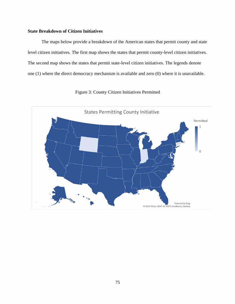
75
State Breakdown of Citizen Initiatives
The maps below provide a breakdown of the American states that permit county and state
level citizen initiatives. The first map shows the states that permit county-level citizen initiatives.
The second map shows the states that permit state-level citizen initiatives. The legends denote
one (1) where the direct democracy mechanism is available and zero (0) where it is unavailable.
Figure 3: County Citizen Initiatives Permitted
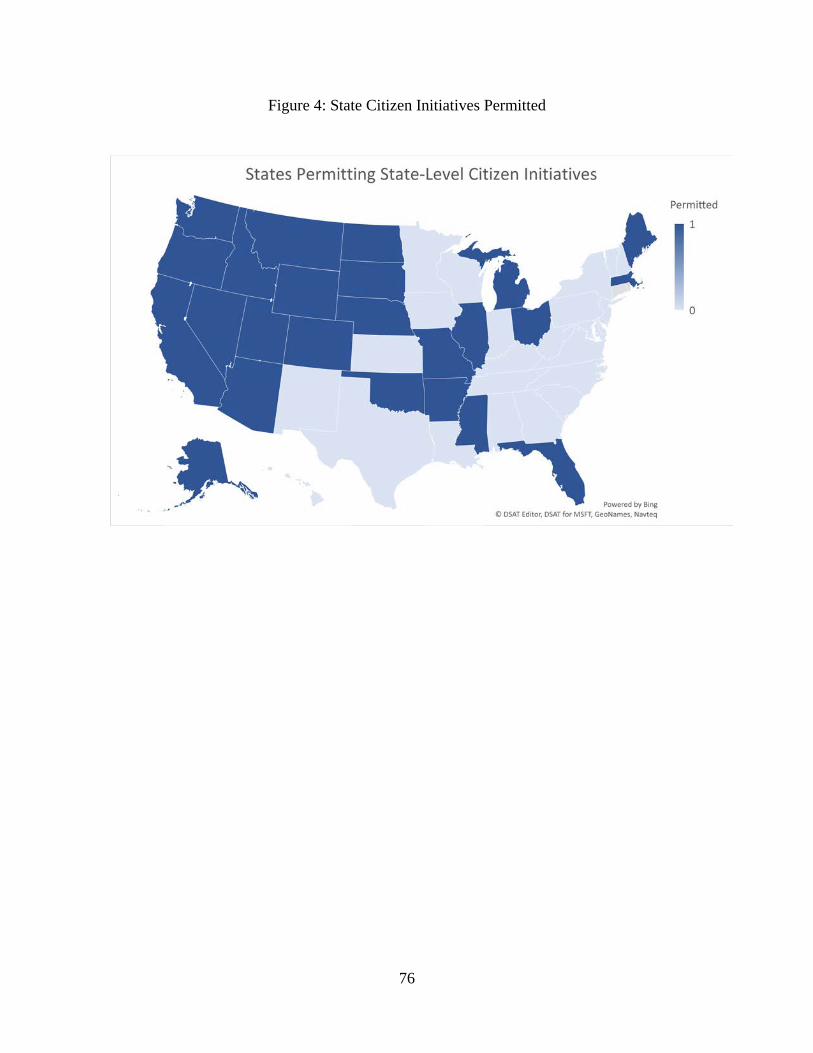
76
Figure 4: State Citizen Initiatives Permitted

77
Methods and Models
This study uses a cross-sectional analysis to examine part I and part II models for each
county in the survey sample. I estimate the models in this study using Stata 14 and SPSS 24. This
section will focus on laying out the methods to estimate both parts I and part II of this
dissertation, i.e., the government structure model and voter turnout model, respectively.
Part I
A prerequisite of ordinary least squares (OLS) regression is that the dependent variable is
continuous. Examining the availability of the initiative requires predicting values that are binary,
i.e., zero or one. Using OLS would violate the assumptions of homoscedasticity, linearity, and
normality (Mehmetoglu, 2016). In this case, using a logistic regression model will give the
probability of the dependent variable having the value of one or zero, given the values of the
independent and control variables (Mehmetoglu, 2016). Subsequently, the logistic model uses
maximum likelihood estimation (MLE) rather than ordinary least squares to estimate the
parameters that would make the data most likely (Mehmetoglu, 2016). I report the odds ratios in
the coefficient tables for chapter four, which is the exponential of the logit.
As Svara (1996) notes, there is very little research on topics that concern the traditional
commission or elected-executive forms of government. Therefore, this research study addresses
both aspects by analyzing the traditional commission form of government in addition to all three
reformed governments, i.e., council-manager, council administrator, and council-elected. For this
study, I use a cross-sectional analysis to study the impact of county government structure on
citizen initiative availability. This procedure has been widely implemented in the public
administration literature (see chapter five on the structure of county government, DeSantis &
Renner, 1996).

78
A major advantage of this research design is that it uses a national sample of 630
American counties as opposed to a small sample of large American counties (e.g., typically less
than 50, see Tekniepe & Stream, 2010). Furthermore, Pammer (1996) advocates for cross-
sectional designs in analyzing county government policymaking decisions. Pammer points out
the significance of three factors that this study meets. First, this study uses a comprehensive
national dataset of county policy measures to ensure representation and generalizability. Second,
this study uses taxes collected per capita and county expenditure per capita as a control measure
to capture a counties’ fiscal health. Third, and finally, this study analyzes the enactment of
citizen initiatives as a long-term policy tool. Citizen initiatives meet the strategic analysis
component put forth by Pammer since its enactment can meet citizen demands for many decades
post-hoc.
This procedure considers state constitutional rules to isolate the effects of government
structure on the availability of the citizen initiative. The effects of government structure,
socioeconomic, and control variables are estimated using maximum likelihood with robust
standard errors to correct for heteroscedasticity (Hill, Griffiths, & Lim, 2008). The robust
standard errors associated with each coefficient corrects for heteroscedasticity by using a
variance matrix more robust than that of ordinary least squares (Farmer, 2017). I conduct the
Cook-Weisberg analysis to test for heteroscedasticity in chapter four, which verifies the
applicability of this procedure.
To examine the government structure model effects, the cross-sectional procedure
involves using the logistic command in Stata 14 to report the odds ratios for predicting the
influence on the availability of the initiative. The dependent variable is the availability of the
citizen initiative at time 𝑡𝑡, and the independent variables include socioeconomic and control
79
variables at 𝑡𝑡 and 𝑡𝑡 − 1 that are anticipated to influence the dependent variable (Choi et al.,
2010). To ensure a proper estimation of the coefficients, the population was logged before
estimating the regression because it is not normally distributed (Choi et al., 2010).
Similar to Moore & Ravishankar (2012), I apply a listwise deletion for counties that did
not respond to key variables. Each model will be checked for outliers by assessing Cook’s D and
leverage based on the recommendations from Adkins & Hill (2011). I also check for
multicollinearity by assessing variance inflation factor values greater than 10 to address any data
transformations that may be necessary (Adkins & Hill, 2011). Finally, I detail the government
structure model below.
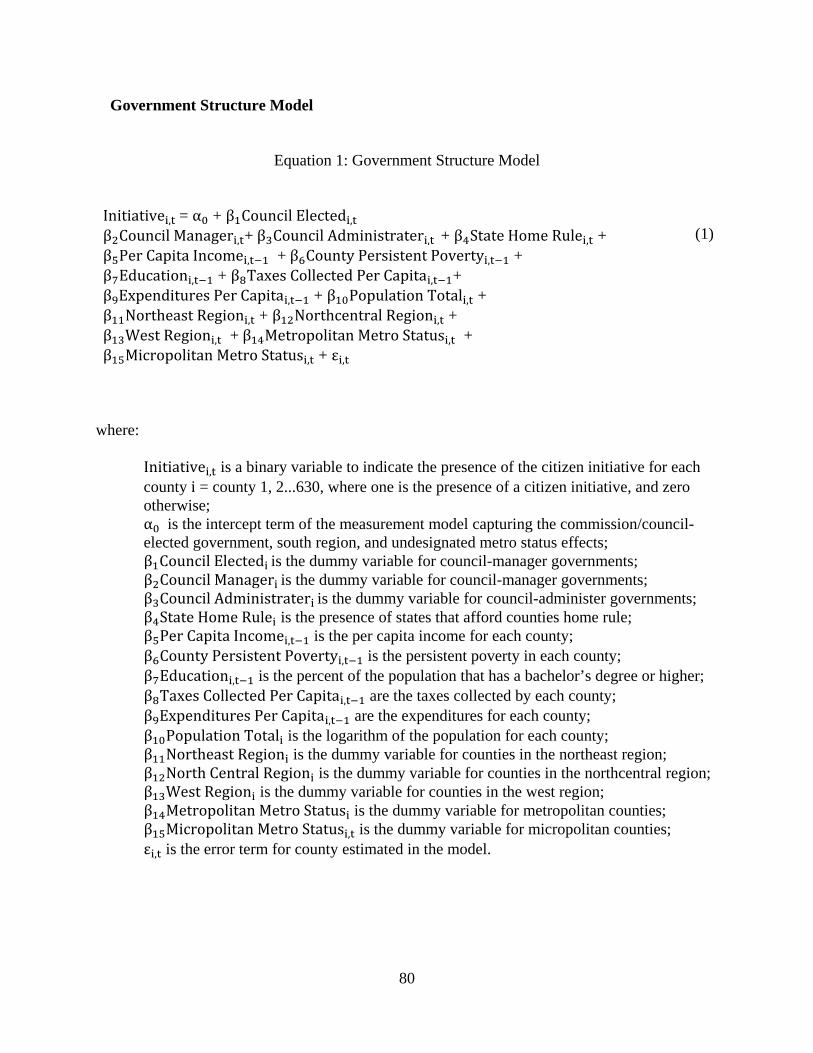
80
Government Structure Model
Equation 1: Government Structure Model
Initiativei,t = α0 + β1Council Electedi,t β2Council Manageri,t+ β3Council Administrateri,t + β4State Home Rulei,t + β5Per Capita Incomei,t−1 + β6County Persistent Povertyi,t−1 + β7Educationi,t−1 + β8Taxes Collected Per Capitai,t−1+ β9Expenditures Per Capitai,t−1 + β10Population Totali,t + β11Northeast Regioni,t + β12Northcentral Regioni,t + β13West Regioni,t + β14Metropolitan Metro Statusi,t + β15Micropolitan Metro Statusi,t + εi,t
(1)
where:
Initiativei,t is a binary variable to indicate the presence of the citizen initiative for each county i = county 1, 2...630, where one is the presence of a citizen initiative, and zero otherwise; α0 is the intercept term of the measurement model capturing the commission/council-elected government, south region, and undesignated metro status effects; β1Council Electedi is the dummy variable for council-manager governments; β2Council Manageri is the dummy variable for council-manager governments; β3Council Administrateri is the dummy variable for council-administer governments; β4State Home Rulei is the presence of states that afford counties home rule; β5Per Capita Incomei,t−1 is the per capita income for each county; β6County Persistent Povertyi,t−1 is the persistent poverty in each county; β7Educationi,t−1 is the percent of the population that has a bachelor’s degree or higher; β8Taxes Collected Per Capitai,t−1 are the taxes collected by each county; β9Expenditures Per Capitai,t−1 are the expenditures for each county; β10Population Totali is the logarithm of the population for each county; β11Northeast Regioni is the dummy variable for counties in the northeast region; β12North Central Regioni is the dummy variable for counties in the northcentral region; β13West Regioni is the dummy variable for counties in the west region; β14Metropolitan Metro Statusi is the dummy variable for metropolitan counties; β15Micropolitan Metro Statusi,t is the dummy variable for micropolitan counties; εi,t is the error term for county estimated in the model.

81
Part II
The voter turnout research design investigates voter turnout by using a combination of
county and state variables. I analyze the county and state level effects by using the 2016
presidential election data. Because individuals of the same counties can react to the same
contextual factors, they may not be independent (Knotts & Haspel, 2006). Based on this
rationale, using a standard ordinary least squares regression would violate the assumption of
uncorrelated errors, leading to a biased hypothesis test (Knotts & Haspel, 2006; Rabe-Hesketh,
2012). Therefore, this study uses a multilevel (MLM) continuous regression model with counties
(level 1) that reside within states (level 2). Thus, similar to Singh (2011), I estimate a multilevel
model in which I fit a unique intercept for each state equation, also referred to as the random
intercept. Specifically, the author uses the mixed command in Stata 14. The author also reports
Huber-White Sandwich robust standard errors to account for the possibility of correlation and
heteroscedasticity within clusters (Knotts & Haspel, 2006). Similar to part I, I conduct the Cook-
Weisberg analysis to test for heteroscedasticity in chapter four to verify the applicability of
robust standard errors.
County-level characteristics such as socioeconomic, demographic, and control variables
compose level 1, whereas measures of state explanations compose level 2. The primary county-
level variable of interest includes the citizen initiative enacted by each county government. Using
the same multilevel model, I include state variables of interest to include the number of citizen
initiatives on the election ballot and interest group monetary contributions to support or oppose
citizen campaigns. The estimation strategy of multilevel modeling borrow strength from other
level 2 factors and improves the ability of the model to draw an inference about state-level
effects by allowing the intercept term to vary by state (C. Tolbert et al., 2009). As Tolbert et al.
82
mentions, multilevel models can account for more of the variance between states than do
traditional regression models, potentially improving the coefficient estimate of the level 1 and
level 2 variables.
Similar studies that use survey data to test voting behavior do not account for the fact that
respondents are often clusters within states by using multilevel modeling (MLM) strategies to
adjust standard errors (e.g., see Lacey, 2005; C. J. Tolbert, McNeal, & Smith, 2003). Using
multilevel models corrects for problems of clustering in the standard errors and accounts for
possible non-constant variances across state contexts (C. Tolbert et al., 2009). Thus, scholars
often ignore the heterogeneity for each state in which voters reside, and therefore rarely take
advantage of multilevel data and the fact that individuals reside in measurable political
environments (Primo et al., 2007). Finally, I detail the voter turnout model below.
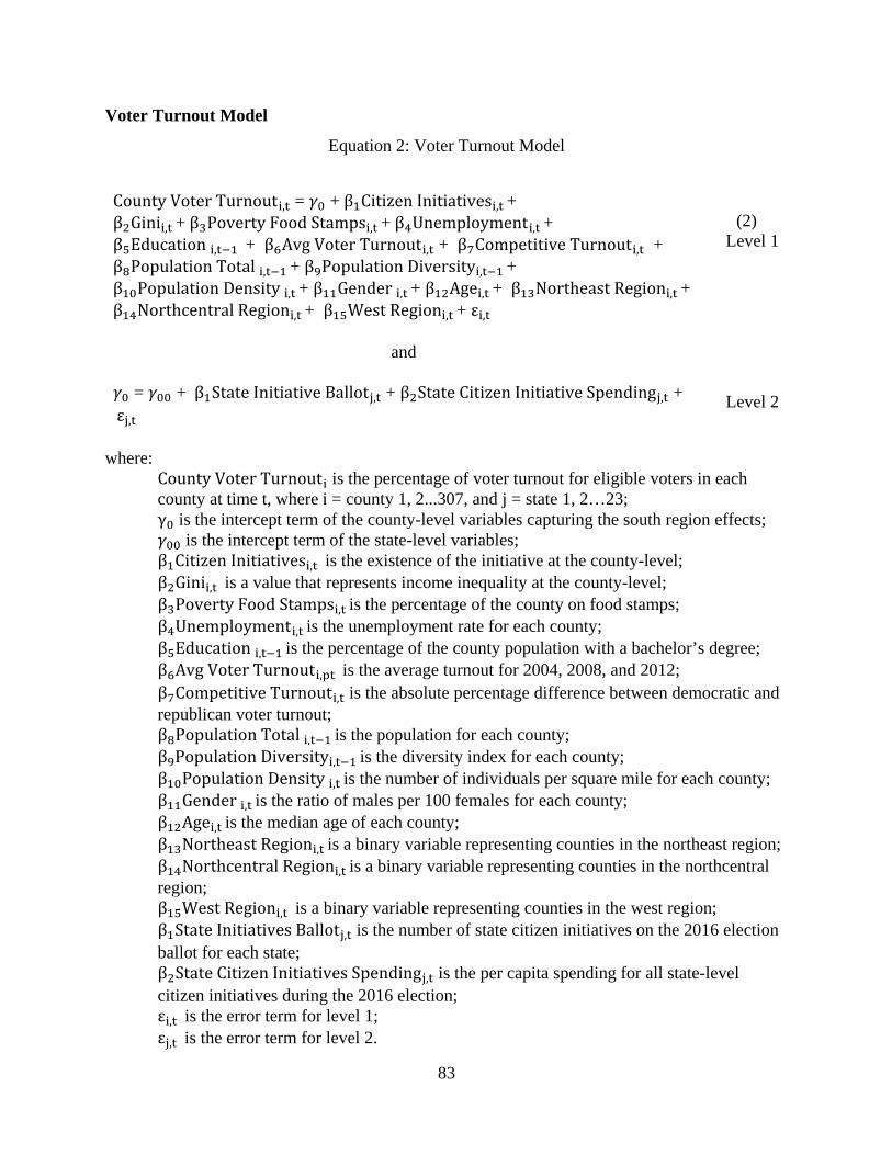
83
Voter Turnout Model
Equation 2: Voter Turnout Model
County Voter Turnouti,t = 𝛾𝛾0 + β1Citizen Initiativesi,t + β2Ginii,t + β3Poverty Food Stampsi,t + β4Unemploymenti,t + β5Education i,t−1 + β6Avg Voter Turnouti,t + β7Competitive Turnouti,t + β8Population Total i,t−1 + β9Population Diversityi,t−1 + β10Population Density i,t + β11Gender i,t + β12Agei,t + β13Northeast Regioni,t + β14Northcentral Regioni,t + β15West Regioni,t + εi,t
and 𝛾𝛾0 = 𝛾𝛾00 + β1State Initiative Ballotj,t + β2State Citizen Initiative Spendingj,t + εj,t
(2)
Level 1 Level 2
where: County Voter Turnouti is the percentage of voter turnout for eligible voters in each county at time t, where i = county 1, 2...307, and j = state 1, 2…23; γ0 is the intercept term of the county-level variables capturing the south region effects; 𝛾𝛾00 is the intercept term of the state-level variables; β1Citizen Initiativesi,t is the existence of the initiative at the county-level; β2Ginii,t is a value that represents income inequality at the county-level; β3Poverty Food Stampsi,t is the percentage of the county on food stamps; β4Unemploymenti,t is the unemployment rate for each county; β5Education i,t−1 is the percentage of the county population with a bachelor’s degree; β6Avg Voter Turnouti,pt is the average turnout for 2004, 2008, and 2012; β7Competitive Turnouti,t is the absolute percentage difference between democratic and republican voter turnout; β8Population Total i,t−1 is the population for each county; β9Population Diversityi,t−1 is the diversity index for each county; β10Population Density i,t is the number of individuals per square mile for each county; β11Gender i,t is the ratio of males per 100 females for each county; β12Agei,t is the median age of each county; β13Northeast Regioni,t is a binary variable representing counties in the northeast region; β14Northcentral Regioni,t is a binary variable representing counties in the northcentral region; β15West Regioni,t is a binary variable representing counties in the west region; β1State Initiatives Ballotj,t is the number of state citizen initiatives on the 2016 election ballot for each state; β2State Citizen Initiatives Spendingj,t is the per capita spending for all state-level citizen initiatives during the 2016 election; εi,t is the error term for level 1; εj,t is the error term for level 2.
84
Chapter 4: Empirical Results
In this chapter, I will review model diagnostics to examine the methods outlined in
chapter three. Then, I will describe the regression results for parts I and part II separately, and to
what degree the evidence supports the hypotheses. I will conclude with model specific post-
estimation procedures and graphical depictions of the models to aid the interpretations.
Part I: Government Structure Model
Model Diagnostics
Test for Omitted Variables
Testing for omitted variables is a crucial step in model specification. Therefore, I conduct
Ramsey's (1969) widely used regression specification error test for omitted variables. A
nonsignificant test means that the researcher can retain the null indicating that there are no
omitted variables. Subsequently, retaining the null hypothesis suggests that the model is
acceptable according to the test (Mehmetoglu, 2016). After running the regression for the
government structure model, I report the following results, F(3,611) = .74, p > .05. This result
suggests that the relevant predictors are included in the model. In other words, the F critical
value result reduces the chance of an endogenous problem where a relevant predictor omitted
may actually explain the outcome variable, i.e., the citizen initiative (Acock, 2013). I fail to
reject the null and infer that the model has adequate specifications. Therefore, I proceed with the
analysis.

85
Cook-Weisberg Test for Heteroskedasticity
Homoscedasticity is the assumption that the error term has constant variance
(Mehmetoglu, 2016). Homoscedasticity is an important assumption since it allows the model to
predict 𝑋𝑋1..𝑛𝑛 values equally well for low values as well as high values on Y , i.e., the county
initiative (Mehmetoglu, 2016). Therefore, I apply the Cook and Weisberg (1983) test for
heteroscedasticity. It is a chi-square test of the null hypothesis that the model has homoscedastic
residuals, so if the p value is less than .05, it means that heteroscedasticity is present. After
running the test, I report the following results.
𝜒𝜒2 (1,𝑁𝑁 = 630) = 5.62,𝑝𝑝 = .0178
The test shows that heteroscedasticity is present. In this case, to correct for
heteroscedasticity, I use the robust standard errors procedure to avoid any biases in the
coefficients (Mehmetoglu, 2016).
Chi-Square Tests
In this section, I will discuss the insight that chi-square tests can provide for part one.
Chi-square tests are useful for examining frequency relationships between two categorical
variables (Field, 2013). Therefore, I employ this test to examine the significance of the
frequencies between the primary dependent (initiative) and independent variables (forms of
government) of interest since these variables are all binary.
First, I provide the frequency distributions of the government form variables. The
frequency output shows that all the governments have fair representation in counties across the
U.S, which is important for model specification as Mehmetoglu (2016) points out. Notably, 25
percent of counties have the council-manager government, 23 percent of counties have the

86
commission government, 10 percent of counties have the council-elected government, and 34
percent of counties have the council-administrator government (see table 4).
Table 4: Government Structure Frequencies
Council-Manager Freq. Percent Valid Cum. 0 486 66.85 72.21 72.21 1 187 25.72 27.79 100
Total 673 92.57 100 Missing 54 7.43
Total 727 100
Commission Freq. Percent Valid Cum. 0 506 69.6 75.19 75.19 1 167 22.97 24.81 100
Total 673 92.57 100 Missing 54 7.43
Total 727 100
Council-Elected Freq. Percent Valid Cum. 0 604 83.08 89.75 89.75 1 69 9.49 10.25 100
Total 673 92.57 100 Missing 54 7.43
Total 727 100
Council-Administrator Freq. Percent Valid Cum. 0 423 58.18 62.85 62.85 1 250 34.39 37.15 100
Total 673 92.57 100 Missing 54 7.43
Total 727 100

87
Now, I consider the chi-squared tables (see table 5). Looking at the output, the
relationship between the initiative and council-elected government is not significant; neither is
the relationship between the initiative and the council-administrator government. However, the
relationship between the initiative and commission government is significant; and the
relationship between the initiative and council-manager government is significant as well. In the
case of the initiative and council-manager government, the results show: 𝜒𝜒2(1,𝑁𝑁 = 631) =
9.33,𝑝𝑝 < .05. More specifically, about 28 percent of council-manager governments have the
county initiative available. In the case of the initiative and commission government, the results
show: 𝜒𝜒2(1,𝑁𝑁 = 631) = 4.53,𝑝𝑝 < .05. Here, about 44 percent of commission governments
have the county initiative available. In the next section, I discuss the multicollinearity results.
Table 5: Government Structure Chi-squared Tests
Council-Administrator Initiative Not Present Present Total
Not Present 254 148 402 63.98 63.25 63.71
Present 143 86 229 36.02 36.75 36.29
Total 397 234 631 100 100 100
Pearson chi-square (1) = .0341, p = .853
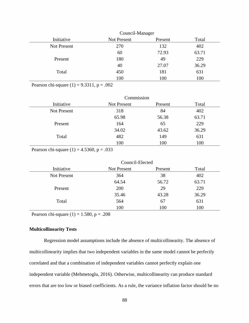
88
Council-Manager Initiative Not Present Present Total
Not Present 270 132 402 60 72.93 63.71
Present 180 49 229 40 27.07 36.29
Total 450 181 631 100 100 100
Pearson chi-square (1) = 9.3311, p = .002 Commission
Initiative Not Present Present Total Not Present 318 84 402
65.98 56.38 63.71 Present 164 65 229
34.02 43.62 36.29 Total 482 149 631
100 100 100 Pearson chi-square (1) = 4.5360, p = .033
Council-Elected
Initiative Not Present Present Total Not Present 364 38 402
64.54 56.72 63.71 Present 200 29 229
35.46 43.28 36.29 Total 564 67 631
100 100 100 Pearson chi-square (1) = 1.580, p = .208
Multicollinearity Tests
Regression model assumptions include the absence of multicollinearity. The absence of
multicollinearity implies that two independent variables in the same model cannot be perfectly
correlated and that a combination of independent variables cannot perfectly explain one
independent variable (Mehmetoglu, 2016). Otherwise, multicollinearity can produce standard
errors that are too low or biased coefficients. As a rule, the variance inflation factor should be no

89
greater than 10 for any independent variable (Field, 2013). Similarly, the tolerance is the
reciprocal of the variance inflation factor (tolerance = 1/VIF) and should be greater than .10
(Field, 2013). The highest and lowest VIF is per capita income at 4.10, and state home rule at
1.89, respectively. For the government structure model, the mean VIF is 1.89 and mean
tolerance is .61. The results from table 6 indicate that there are no serious multicollinearity issues
present in the government structure model.
Table 6: Government Structure Model Multicollinearity Results
Variable VIF Tolerance Per Capita Income 4.010 0.249 Education 3.860 0.259 Expenditures Per Capita 2.310 0.432 Taxes Collected Per Capita 2.190 0.457 Council-Manager 1.980 0.504 Council-Administrator 1.800 0.556 Metropolitan Status 1.600 0.624 Population 1.530 0.654 Northeast Region 1.440 0.695 West Region 1.370 0.732 Council-Elected 1.340 0.747 Micropolitan Status 1.340 0.748 County Initiative 1.240 0.805 Northeast Region 1.150 0.868 State Home Rule 1.140 0.879 Mean 1.890 0.614 Notes. Based on 630 observations. Variables with VIF < 1.00 excluded.

90
Pairwise Correlations
In this section, I review pairwise correlations for the main hypotheses regarding the
government structure model (see table 7). The following pairwise correlation coefficient matrix
indicates both the strength and significant of each relationship. This matrix can be useful to
describe how variables covary with each other (Field, 2013). I only print the relationships that
were significant at p < 0.5. Accordingly, of the variables analyzed for the main hypotheses, there
are 16 significant relationships. The strongest positive relationship exists between income and
education at .832, whereas the strongest negative relationship exists between the council-
manager and council-administrator forms of government at -.477.
Table 7: Government Structure Correlations
Variables IN Com. CE CM CA HR Inc. Pov. County Initiative (IN) 1.000 Commission (COM) 0.085 1.000 Council-Elected (CE) -0.194 1.000 Council-Manager (CM) -0.122 -0.356 -0.210 1.000 Council-Admin (CA) -0.442 -0.260 -0.477 1.000 Home Rule (HR) 0.159 1.000 Income (Inc.) -0.148 0.141 1.000 Poverty (Pov.) -0.362 1.000 Education (Educ) -0.143 0.185 0.832 -0.207 Notes. Pairwise correlations with coefficients p < .05 only reported. Control variables excluded.
Descriptive Statistics
The 2014 ICMA survey collected responses from 750 counties across the United States.
After accounting for missing data and the adjustment for two states restricting county-level
initiatives, the final sample uses 672 county initiative observations for the dependent variable
(see table 8). The average per capita income in the samples $24,578, with a minimum of $9,688
and a maximum of $51,851. The persistent poverty variable is a measure between zero and one

91
for each county that has had 20 percent or more of its population living in poverty over the past
30 years. Accordingly, the persistent poverty mean is .10, indicating that relatively few counties
in the sample have experienced severe long-run poverty. On average, about 13 percent of the
counties in the sample have a population with a bachelor’s degree or higher. Finally, the means
for taxes collected per capita and expenditures per capita are relatively equal, at 1.38 and 1.41,
respectively. The differences most likely due to intergovernmental funding (Farmer, 2017).
Table 8: Government Structure Descriptive Statistics
Variable Obs. Mean Std. Dev. Min Max County Initiative 672 - - 0.00 1.00 Commission 673 - - 0.00 1.00 Council-Elected 673 - - 0.00 1.00 Council-Manager 673 - - 0.00 1.00 Council-Administrator 673 - - 0.00 1.00 State Home Rule 727 - - 0.00 1.00 Per Capita Income 727 24,578.94 6,071.74 9,688.00 51,851.00 Persistent Poverty 727 0.10 0.30 0.00 1.00 Education 727 13.25 5.92 3.90 40.41 Taxes Collected Per Capita 726 1.38 1.87 0.03 20.69 Expenditures Per Capita 726 1.41 1.38 0.03 18.48 Log Population 727 10.44 1.46 5.61 16.12 Northeast Region 727 - - 0.00 1.00 Northcentral Region 727 - - 0.00 1.00 West Region 727 - - 0.00 1.00 South Region 727 - - 0.00 1.00 Metropolitan Status 727 - - 0.00 1.00 Micropolitan Status 727 - - 0.00 1.00 Undesignated Status 727 - - 0.00 1.00 Notes. Obs. = total observations. Std. Dev. = Standard Deviation
92
Logistic Model 1 Interpretations
As discussed in chapter three, I report the odds ratios for the coefficients in the
government structure model. The odds ratios report the exponential logit, which indicates a
change in odds (county initiative = 1) for a move one step up on the independent variable
(depending if it is categorical or continuous) (Mehmetoglu, 2016). In other words, an odds ratio
of greater than one indicates that it is more likely to happen, whereas a value less than one
indicates that it is less likely to happen. Therefore, in this scenario, an odds ratio of 1 means that
there is no change (i.e., no effect of the independent variable on the dependent variable)
(Mehmetoglu, 2016). The value 1 is the equivalent to the coefficient of 0 in ordinary least
squares (OLS). Therefore an odds ratio greater than 1 means that the effect is positive, while an
odds ratio less than 1 means that the effect is negative (Mehmetoglu, 2016).
Model 1 reports a pseudo R-square value of .105, which indicates about 10.5 percent of
the variance in the initiative is explained by the independent and control variables (see table 9).
For this model, I refer to the z-statistic for the significance of variables, also known as the Wald
statistic following a (χ2) chi-square distribution. Hypothesis 1 is largely supported with some
caveats detailed below. Hypothesis 1 test the probability of association between government
structure and the availability of the initiative. Using the commission government as a reference
group, the odds ratios for the reformed governments are council-elected (1.079), council-
manager (.518), and council-administrator (.740). The council-manager coefficient is significant,
whereas the council-elected and council-administrator coefficients are not. Given the .518 odds
ratio of the council-manager government, the odds for a county with the initiative decreases by
48 percent for each county that has a council manager government as opposed to not having this
government in place (i.e., 1 as opposed to 0). Although not significant, the council-elected odds

93
ratio of 1.079 indicates that the odds for counties with the initiative increase by 7.9 percent for a
county with the council-elected form of government. I also explore hypothesis one in model two
and three further, which will be discussed below. In sum, there is evidence showing that the
initiative is more likely to exist with counties that emphasize elected representatives as opposed
to appointed representatives, i.e., at least relative to the commission and council-manager
governments.
Hypothesis 2 is supported by solid evidence showing that counties would state home rule
are more inclined to have the initiative available. The odds ratio coefficient for state home rule is
1.807, with a p-value < .01. In this case, the odds for counties with the initiative increases by
almost 81 percent for each county that has the state home rule available. Hypothesis 2 provides
insight into the ability of counties to use institutional arrangements for the benefit of serving
citizens with more ways to initiate legislation. Hypothesis 3 test the association between per
capita income and the availability of the initiative. As such, hypothesis 3 is significant, however,
the effect is minimal since the odds ratio was 1.0006 (total coefficient abbreviated in the table).
Subsequently, higher per capita income is only slightly associated with counties that have the
initiative available.
Hypothesis 4 testing persistent poverty is not significant. Interestingly, however, it is in
the opposite expected direction. The odds ratio for persistent poverty is 1.201, indicating that the
odds for counties with the initiative increase by 21 percent for each unit of persistent poverty
increase. In other words, the odds for counties with the initiative increases by .21% for each .1
unit increase in persistent poverty on a scale from 0 to 1. This result could be due to community
activism since the initiative can be used for a wide range of policymaking. Specifically, the
initiative can include not just economic issues that concern the elite, but rather social issues that
94
concern poverty-stricken areas or educational issues (Carswell, 2005). For example,
policymakers may have decided that giving citizens in low-income areas the ability to initiate
rent control would better serve the population (Bowler et al., 1998).
Hypothesis 5 testing the association between education and the initiative is significant as
well. However, the odds ratio coefficient for education is .937, indicating that the odds for
counties with the initiative decrease by 6.3 percent for each 1 percent increase in the county’s
population of individuals that have a bachelor’s degree or higher. While this is in the opposite
direction, it may be explained by individuals that have the knowledge and wherewithal of the
initiative but would rather deprive citizens of the ability to initiate legislation on their own
behalf. Such a power grab may occur since some policymakers often want to hold sway over
policymaking rather than bestow it to the citizens. Subsequently, policymakers that are more
knowledgeable about the power of the initiative would want to maintain its benefits (Dubois &
Feeney, 1998).
Control Variables
The control variables serve a purpose to avoid spurious results and increase the ability to
provide causal inference (Mehmetoglu, 2016). In this case, the control variables included in this
model have been widely cited in past literature concerning government structure (i.e., see chapter
two). Interestingly, taxes collected and expenditures for each county on a per capita basis have
no significant associations with the availability of the initiative. The rest of the control variables
are also not significant with the exception of the northcentral and west regions. I will the discuss
implications of the region coefficients more below.
On the other hand, the region results meet expectations. As noted, chapter two discusses a
wide range of examples of where the progressive west was more inclined to use the initiative

95
with a particular emphasis on the state of California. Such progressivism shows up in the model
with the west region odds ratio coefficient of 6.38, meaning that the odds for counties with the
initiative are almost 5.5 times more likely in the west region when compared to the south region
(reference group). Likewise, the south region has been plagued with misaligned policies that
deprive underrepresented citizens the power to initiate legislation. I discuss these examples in
chapter two, but a brief list would include Jim Crow laws and policies that were in direct conflict
with the civil rights movement during the 1960s.
The northcentral region is also significant within odds ratio coefficient of 1.71, meaning
that the odds of counties with the initiative increase by 71 percent for counties in this region.
States such as Michigan are more unionized; and therefore, unions may be partially responsible
for the efforts to put policymakers in charge that enact the citizen initiative for counties in this
area. For example, in 1996, labor unions placed initiatives on California’s ballot that would raise
the minimum wage and regulate campaign contributions (Bowler et al., 1998).
Logistic Model 2 and 3 Interpretations
Mehmetoglu (2016) points out the importance of conducting a sensitivity analysis by
making relevant changes to model specifications. The rationale is to assess if the results are
robust to different sources of uncertainty (Mehmetoglu, 2016). Therefore, I run different versions
of the government model with one modification for each estimation. Mehmetoglu (2016) also
points out that the second option to test for the main effects of governments on the initiative is to
examine a linear combination of coefficients. The author performed this procedure as well.
However, to ease interpretation, I present the logistic models as opposed to producing a different
table of linear combinations since the tests produce the same results.
96
The only difference between model 1 and model 2 is the omission of the council-elected
form of government while keeping all other variables the same (see table 10). I conduct this test
for two primary reasons: 1) examine any significant changes in coefficients or p values, and 2)
allow the commission and council-elected government to serve as one group (reference group) in
the second model based on the theoretical considerations discussed in chapter two. Subsequently,
the comparison now examines the probability of the council-manager and council-administrator
governments relative to the commission and council-elected governments. In this case, for model
2, the results show that the council-manager form of government is less likely to be present with
an odds ratio of .504 and p-value < .05. Similarly, the council-administrator government is also
less likely to be present with an odds ratio .722; however, the p value is > .05.
In model 3, I make one modification by allowing the council-elected form of government
to serve as a reference group (see table 11). This modification is more for interpreting hypothesis
one as opposed to a sensitivity analysis. Nonetheless, I provide this table as a measure to increase
the evidence in support of hypothesis one. In model one, I allow the commission government to
serve as the reference group measuring the mean differences between the other three
governments, i.e., elected, manager, and administrator governments. Therefore, in model 3, I can
compare the mean differences between the other three governments in the regression model, i.e.,
commission, manager, and administrator governments. This model also shows the council
manager is less likely to be associated with the initiative when compared to the council-elected
form of government given an odds ratio of .480 and a p-value < .05. In sum, model 2 and 3 offer
another line of support for hypothesis 1 showing that there is a strong association between
elected bodies of government and the initiative.

97
Logistic Model 4 and 5 Interpretations
In model four, I further investigate the notion of high-powered versus low powered
election incentives. Recall from chapter two that both the commission and council-elected
forms of county government emphasize elected representatives as principal components of
each respective government. This is in stark contrast to the council-administrator and council-
manager governments that have low powered election incentives due to their professional
focus and little emphasis on elections for county board members (Svara, 1996). Therefore,
using this logic with the theoretical nature of new institutionalism, the researcher creates two
new variables. A variable that combines the commission and council-elected governments and
a variable that combines the council-administrator and council manager governments. Letting
the commission and council-elected government serve as the reference group, the researcher
conducts another analysis on the government structure model. The results are largely
consistent with the previous models supporting hypothesis one. As such, the council-manager
and council-administrator combined variable show an odds ratio coefficient of .639 at p < .05.
Therefore, the citizen initiative has a higher association with high-powered elected
governments relative to low powered elected governments.
Finally, as noted in chapter two, the state of California has one of the most active
electorates for citizen initiatives (Goebel, 2002). From Ventura county to Napa Valley,
California voters have voiced their opinion on a range of issues that span from tax issues to
land amendments (Zimmerman, 2015). Given this hotbed of citizen initiatives, the researcher
runs the government structure analysis for model five while removing California from the
analysis. The model now includes 45 states and 611 counties. The researcher retains the newly
created variables combining high-powered and low powered elected governments. In this case,

98
the results continue to be consistent. The council-manager and council-administrator combined
variable shows an odds ratio coefficient of .606 at p < .05. Therefore, the citizen initiative has
a higher association with high-powered elected governments relative to low powered elected
governments.
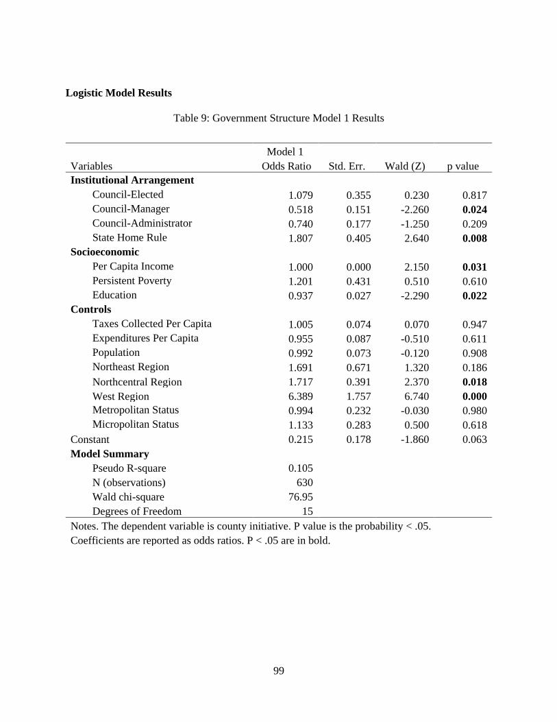
99
Logistic Model Results
Table 9: Government Structure Model 1 Results
Model 1 Variables Odds Ratio Std. Err. Wald (Z) p value Institutional Arrangement
Council-Elected 1.079 0.355 0.230 0.817 Council-Manager 0.518 0.151 -2.260 0.024 Council-Administrator 0.740 0.177 -1.250 0.209 State Home Rule 1.807 0.405 2.640 0.008
Socioeconomic Per Capita Income 1.000 0.000 2.150 0.031 Persistent Poverty 1.201 0.431 0.510 0.610 Education 0.937 0.027 -2.290 0.022
Controls Taxes Collected Per Capita 1.005 0.074 0.070 0.947 Expenditures Per Capita 0.955 0.087 -0.510 0.611 Population 0.992 0.073 -0.120 0.908 Northeast Region 1.691 0.671 1.320 0.186 Northcentral Region 1.717 0.391 2.370 0.018 West Region 6.389 1.757 6.740 0.000 Metropolitan Status 0.994 0.232 -0.030 0.980 Micropolitan Status 1.133 0.283 0.500 0.618
Constant 0.215 0.178 -1.860 0.063 Model Summary
Pseudo R-square 0.105 N (observations) 630 Wald chi-square 76.95 Degrees of Freedom 15
Notes. The dependent variable is county initiative. P value is the probability < .05. Coefficients are reported as odds ratios. P < .05 are in bold.

100
Table 10: Government Structure Model 2 Results
Model 2 Variables Odds Ratio Std. Err. Wald (Z) p value Institutional Arrangement
Council-Elected Council-Manager 0.504 0.134 -2.570 0.010 Council-Administrator 0.722 0.155 -1.520 0.129 State Home Rule 1.807 0.406 2.640 0.008
Socioeconomic Per Capita Income 1.000 0.000 2.180 0.029 Persistent Poverty 1.200 0.431 0.510 0.612 Education 0.937 0.026 -2.300 0.021
Controls Taxes Collected Per Capita 1.005 0.074 0.070 0.943 Expenditures Per Capita 0.955 0.087 -0.510 0.612 Population 0.992 0.073 -0.120 0.908 Northeast Region 1.684 0.668 1.310 0.189 Northcentral Region 1.708 0.388 2.350 0.019 West Region 6.360 1.742 6.750 0.000 Metropolitan Status 0.999 0.232 -0.010 0.995 Micropolitan Status 1.138 0.284 0.520 0.604
Constant 0.219 0.179 -1.860 0.063 Model Summary
Pseudo R-square 0.10 N (observations) 630 Wald chi-square 76.96 Degrees of Freedom 14
Notes. The dependent variable is county initiative. P value is the probability < .05. Coefficients are reported as odds ratios. P < .05 are in bold.

101
Table 11: Government Structure Model 3 Results
Model 3 Variables Odds Ratio Std. Err. Wald (Z) p value Institutional Arrangement
Commission 0.927 0.305 -0.230 0.817 Council-Manager 0.480 0.163 -2.160 0.031 Council-Administrator 0.686 0.212 -1.220 0.223 State Home Rule 1.807 0.405 2.640 0.008
Socioeconomic Per Capita Income 1.000 0.000 2.150 0.031 Persistent Poverty 1.201 0.431 0.510 0.610 Education 0.937 0.027 -2.290 0.022
Controls Taxes Collected Per Capita 1.005 0.074 0.070 0.947 Expenditures Per Capita 0.955 0.087 -0.510 0.611 Population 0.992 0.073 -0.120 0.908 Northeast Region 1.691 0.671 1.320 0.186 Northcentral Region 1.717 0.391 2.370 0.018 West Region 6.389 1.757 6.740 0.000 Metropolitan Status 0.994 0.232 -0.030 0.980 Micropolitan Status 1.133 0.283 0.500 0.618
Constant 0.232 0.198 -1.710 0.087 Model Summary
Pseudo R-square 0.105 N (observations) 630.000 Wald chi-square 76.950 Degrees of Freedom 15.000
Notes. The dependent variable is county initiative. P value is the probability < .05. Coefficients are reported as odds ratios. P < .05 are in bold.

102
Table 12: Government Structure Model 4 Results
Model 4 Variables Odds Ratio Std. Err. Wald (Z) p value Institutional Arrangement
Council-Manager/Admin 0.639 0.129 -2.220 0.026 State Home Rule 1.834 0.415 2.680 0.007
Socioeconomic Per Capita Income 1.000 0.000 2.200 0.028 Persistent Poverty 1.211 0.434 0.530 0.593 Education 0.935 0.026 -2.430 0.015
Controls Taxes Collected Per Capita 1.005 0.070 0.070 0.947 Expenditures Per Capita 0.941 0.084 -0.670 0.501 Population 0.990 0.073 -0.140 0.892 Northeast Region 1.844 0.712 1.580 0.113 Northcentral Region 1.825 0.397 2.760 0.006 West Region 6.479 1.776 6.820 0.000 Metropolitan Status 0.986 0.228 -0.060 0.953 Micropolitan Status 1.131 0.282 0.490 0.622
Constant 0.221 0.181 -1.850 0.064 Model Summary
Pseudo R-square 0.102 N (observations) 630 Wald chi-square 73.760 Degrees of Freedom 13.000
Notes. The dependent variable is county initiative. P value is the probability < .05. Coefficients are reported as odds ratios. P < .05 are in bold.

103
Table 13: Government Structure Model 5 Results
Model 5 Variables Odds Ratio Std. Err. Wald (Z) p value Institutional Arrangement
Council-Manager/Admin 0.606 0.121 -2.510 0.012 State Home Rule 2.194 0.507 3.400 0.001
Socioeconomic Per Capita Income 1.000 0.000 1.880 0.060 Persistent Poverty 1.244 0.439 0.620 0.537 Education 0.945 0.027 -1.960 0.051
Controls Taxes Collected Per Capita 1.014 0.069 0.210 0.836 Expenditures Per Capita 0.915 0.084 -0.970 0.334 Population 0.921 0.073 -1.040 0.298 Northeast Region 1.962 0.763 1.730 0.083 Northcentral Region 1.799 0.398 2.660 0.008 West Region 4.459 1.333 5.000 0.000 Metropolitan Status 0.962 0.227 -0.160 0.869 Micropolitan Status 1.193 0.296 0.710 0.476
Constant 0.488 0.424 -0.830 0.409 Model Summary
Pseudo R-square 0.095 N (observations) 611.000 Wald chi-square 67.720 Degrees of Freedom 13.000
Notes. The dependent variable is county initiative. P value is the probability < .05. Coefficients are reported as odds ratios. P < .05 are in bold.

104
As discussed, the odds ratio indicates by how many percent the odds for the dependent
variable (county initiative) increase for one unit increase in the independent variable. For
example, in model 1, with regard to the council manager and initiative, the odds ratio is eb=
e−.66 = .52. As described above, this indicates that the effect of the council manager form of
government is negative on the probability of the county initiative availability. Although I use
odds ratio to discuss the government structure model interpretations, I provide table 14 as an
additional reference for each independent and control variable.
Table 14: Government Structure Coefficient Interpretations
Variable B z P > z eb eb∗Sd(x) Sd(x) Council-Elected 0.08 0.23 0.82 1.08 1.02 0.31 Council-Manager -0.66 -2.26 0.02 0.52 0.74 0.45 Council-Administrator -0.30 -1.26 0.21 0.74 0.86 0.48 State Home Rule 0.59 2.64 0.01 1.81 1.28 0.42 Per Capita Income 0.00 2.15 0.03 1.00 1.45 6242.26 Consistent Persistent Poverty 0.18 0.51 0.61 1.20 1.06 0.30 Education -0.06 -2.29 0.02 0.94 0.68 6.06 Taxes Collected Per Capita 0.00 0.07 0.95 1.00 1.01 1.94 Expenditures Per Capita -0.05 -0.51 0.61 0.95 0.94 1.45 Population -0.01 -0.12 0.91 0.99 0.99 1.49 Northeast Region 0.53 1.32 0.19 1.69 1.14 0.24 Northcentral Region 0.54 2.37 0.02 1.72 1.30 0.48 West Region 1.85 6.74 0.00 6.39 2.04 0.38 Metropolitan Status -0.01 -0.03 0.98 0.99 1.00 0.48 Micropolitan Status 0.12 0.50 0.62 1.13 1.05 0.42 Notes. Based on model 1, N = 630 observations; b = raw coefficient; z = z-score for test of b=0; p > z = p-value for z-test; eb= exp(b) = factor change in odds for unit increase in X; eb∗Sd(x) = change in odds for SD increase in X; Sd(x)= standard deviation of x.
105
Goodness of Fit Test
After carrying out the analysis, I performed the Hosmer-Lemeshow goodness of fit test to
examine the explanatory power of the variables predicting the initiative. This test examines
whether the observed 0 or 1 values on the dependent variable match the expected zero or one
values based on the number of covariate patterns in the data (Mehmetoglu, 2016). In particular,
the test is appropriate if the number of covariate patterns is close to the number of observations
(Hosmer, Lemeshow, & Sturdivant, 2013). A significant value means that the researcher should
reject the model, while p > .05 indicates that the model fits reasonably well (Mehmetoglu, 2016).
Based on the analysis of model one, the test shows 630 observations and 627 covariate patterns,
with a Pearson 𝜒𝜒2 (𝑁𝑁 = 611) = 622.98,𝑝𝑝 = .3596. Subsequently, the test shows that the model
fits the data well. In the next section, I discuss the marginal probabilities for hypothesis 1 based
on the government structure model.
Council-Manager Predictions
In figure 5 below, I produce a plot showing the marginal probabilities for the council-
manager government, keeping all other variables at their minimum, mean, and maximum values
(Mehmetoglu, 2016). I focus on the council manager form of government since it was
statistically significant in all three models. The purpose is to predict the probability of the
initiative for given values of the council-manager variable. In the plot below, the redline
represents the probability of the initiative for having the council manager government (value of
one) and not having the council manager government (value of zero). As expected, the council
manager government slope is indeed negative given the odds ratio of .518.
Test one shows that a county has a 39 percent chance of having the initiative when the
county does not have the council-manager form of government. Test two shows that a county has

106
a 34.8 percent chance of having the initiative when the council-manager variable is at its mean,
i.e., the middle part of the redline. Test three shows that a county has a 25 percent chance of
having the initiative when the county has the council-manager form of government. The tests in
table 15 reflect the calculated probabilities for the middle redline only. Finally, the green line
represents all covariate values at their maximum, whereas the blue line represents all covariate
values at their minimum (refer to descriptive statistics as a reference).

107
Figure 5: Marginal Probabilities for Council-Manager Government
Table 15: Council-Manager Prediction
Council Manager Probability Margin Std. Err. Z P > Z Lower 95% Upper 95% Test 1 (min) 0.390 0.028 14.020 0.000 0.337 0.446 Test 2 (mean) 0.348 0.020 17.100 0.000 0.308 0.388 Test 3 (max) 0.250 0.042 5.910 0.000 0.167 0.333 Notes. Number of observations = 630
.2.4
.6.8
Prob
abilit
y of
Initi
ativ
e
0.00 0.20 0.40 0.60 0.80 1.00Council-Manager Government
Other variables at minimum Other variables at meanOther variables at maximun

108
Part II: Voter Turnout Model
In part two, I apply many of the same diagnostic tests for the voter turnout model as in
part one. Therefore, I omit many of the full definitions for the sake of brevity. However, I report
all relevant descriptive and test statistics. The reader can refer back to part I as a reference for
full definitions.
Model Diagnostics
Test for Omitted Variables
Similar to part one, I conduct Ramsey's (1969) widely used regression specification error
test for omitted variables. A nonsignificant test means that the researcher can retain the null of no
omitted variables, indicating that the model is acceptable according to the test (Mehmetoglu,
2016). After running the regression for the voter turnout model, the test produces the following
results, F(3,286) = .34, p > .05. I fail to reject the null and infer that the model has adequate
specifications. Therefore, I proceed with the analysis.
Cook-Weisberg Test for Heteroskedasticity
Similar to part one, I apply the Cook and Weisberg (1983) test for heteroscedasticity. It is
a chi-square test of the null hypothesis that the model has homoscedastic residuals, so if the p
value is less than .05, it means that heteroscedasticity is present. After running the test, I report
the following test statistic below.
𝜒𝜒2 (1,𝑁𝑁 = 307) = 15.74,𝑝𝑝 < .001
In this case, to correct for heteroscedasticity, I use the robust standard errors procedure to avoid
any bias in the coefficients (Mehmetoglu, 2016).

109
Multicollinearity Tests
Regression model assumptions include the absence of multicollinearity. The absence of
multicollinearity implies that two independent variables in the same model cannot be perfectly
correlated and that a combination of independent variables cannot perfectly explain one
independent variable (Mehmetoglu, 2016). Otherwise, multicollinearity can produce standard
errors that are too low or biased coefficients. The results from table 16 indicate that there are no
serious multicollinearity issues present in the model given the highest VIF of 3.82 and lowest
VIF of 1.22, for state citizen spending and gender, respectively. For the voter turnout model, the
mean VIF is 2.22 and mean tolerance is .50.
Table 16: Voter Turnout Multicollinearity Results
Variable VIF Tolerance State Citizen Spending 3.820 0.262 State Citizen Initiatives 3.420 0.292 Food Stamp Population 3.350 0.298 Food Stamp Population 3.060 0.327 Educational Attainment 3.030 0.330 Population Diversity 2.210 0.452 Past Average Voter Turnout 2.180 0.459 Northcentral Region 2.150 0.465 Unemployment Rate 1.990 0.503 Median Age 1.860 0.537 Population Density 1.820 0.550 Population Total 1.720 0.582 Northeast Region 1.680 0.595 Competitive Voter Turnout 1.580 0.631 Gini Coefficient 1.540 0.648 Citizen Initiative 1.230 0.815 Gender 1.220 0.818 Means 2.227 0.504
Notes. Based on 307 observations.
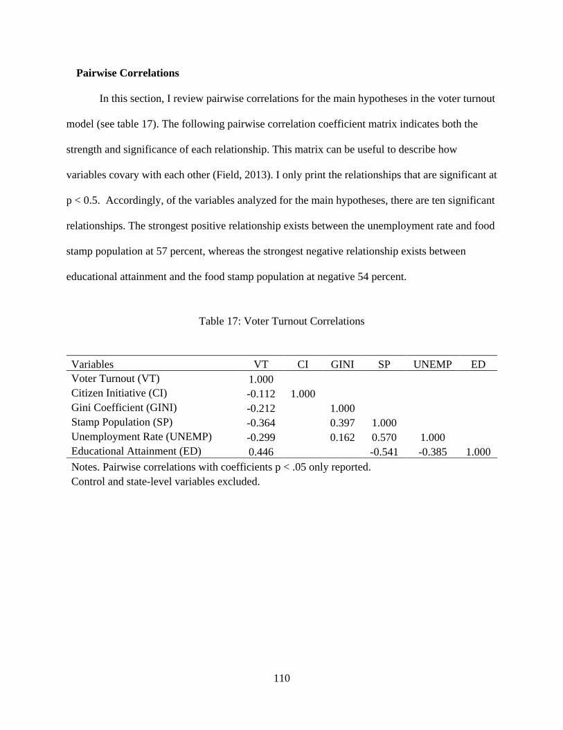
110
Pairwise Correlations
In this section, I review pairwise correlations for the main hypotheses in the voter turnout
model (see table 17). The following pairwise correlation coefficient matrix indicates both the
strength and significance of each relationship. This matrix can be useful to describe how
variables covary with each other (Field, 2013). I only print the relationships that are significant at
p < 0.5. Accordingly, of the variables analyzed for the main hypotheses, there are ten significant
relationships. The strongest positive relationship exists between the unemployment rate and food
stamp population at 57 percent, whereas the strongest negative relationship exists between
educational attainment and the food stamp population at negative 54 percent.
Table 17: Voter Turnout Correlations
Variables VT CI GINI SP UNEMP ED Voter Turnout (VT) 1.000 Citizen Initiative (CI) -0.112 1.000 Gini Coefficient (GINI) -0.212 1.000 Stamp Population (SP) -0.364 0.397 1.000 Unemployment Rate (UNEMP) -0.299 0.162 0.570 1.000 Educational Attainment (ED) 0.446 -0.541 -0.385 1.000 Notes. Pairwise correlations with coefficients p < .05 only reported. Control and state-level variables excluded.

111
Descriptive Statistics
Based on the literature discussed in chapter two (Bowler et al., 1998; Cebulam, 2008; C.
Tolbert et al., 2009) the voter turnout model is estimated for 23 states (24 states except for
Alaska since county voter turnout data was not available). Therefore, the voter turnout model
uses 331 observations for the primary dependent variable of voter turnout (see table 18). The
mean voter turnout for counties in the sample is 57.5 percent, with a minimum of 31 percent and
a maximum of 85 percent. The unemployment rate for the sample is roughly 8 percent. A little
more than 13 percent of the population for each county has a bachelor’s degree or higher. The
mean for the past average voter turnout is 57.7 percent for the 2004, 2008, and 2012 presidential
elections, which is about .2 percent higher than the 57.5 percent turnout for the 2016 presidential
election. The median age is a little more than 41. The mean for the average number of state
citizen initiatives on the ballot in the 2016 election is 2.88, whereas about $4.70 on a per capita
basis was spent on campaigns either supporting or opposing state citizen initiatives.

112
Table 18: Voter Turnout Descriptive Statistics
Variable Obs. Mean Std. Dev. Min Max Voter Turnout 331 0.575 0.096 0.310 0.850 Citizen Initiative 318 - - 0.000 1.000 Gini Coefficient 343 0.443 0.034 0.330 0.530 Food Stamp Population 343 14.695 7.237 1.120 45.140 Unemployment Rate 343 8.055 3.023 2.000 26.000 Educational Attainment 343 13.285 5.899 4.030 40.410 Past Average Voter Turnout 343 0.577 0.100 0.300 0.850 Competitive Voter Turnout 343 0.372 0.205 0.001 0.864 Population Total 343 0.012 0.057 0.000 1.006 Population Diversity 343 16.170 15.534 0.000 78.920 Population Density 343 0.039 0.100 0.000 1.134 Gender 343 100.749 13.442 83.000 258.000 Median Age 343 41.233 5.654 27.000 60.000 Northeast Region 343 - - 0.000 1.000 Northcentral Region 343 - - 0.000 1.000 West Region 343 - - 0.000 1.000 South Region 343 - - 0.000 1.000 State Citizen Initiatives 343 2.880 3.689 0.000 14.000 State Citizen Spending 343 4.702 5.828 0.000 17.310 Notes. (-) denotes dummy variables. Obs. indicates the number of observations.
Trellis Graph by State
In figure 6, I produce a trellis graph containing the plots for all 23 states used in the voter
turnout model analysis. I examine the graphs due to the multilevel model considerations
discussed in chapter 3. The trellis graph is useful since you can see the fitted line for each state
based on the county-level citizen initiative predictor (Rabe-Hesketh, 2012). Based on the results,
many of the fitted lines have negative slopes for the county initiative. I investigate these results
further in the following sections.

113
Figure 6: Trellis Graph of County Initiative by State
.2.4
.6.8
.2.4
.6.8
.2.4
.6.8
.2.4
.6.8
.2.4
.6.8
0 .5 1 0 .5 1
AR AZ CA CO FL
ID IL ME MI MO
MS MT ND NE NV
OH OK OR SD UT
WA WY
Cou
nty
Vote
r Tur
nout
County Initiative Availability
114
Likelihood Ratio Test
As discussed in Chapter three, there are several reasons to consider a multilevel model
when fitting nested variables, i.e., counties within states. However, the first point of order is
carrying out a test to determine the viability of using the multilevel model. To address this task, I
use the log-likelihood ratio test to isolate the impact of the state effects (Rabe-Hesketh, 2012).
Therefore, I examine the maximum likelihood estimation on the county voter turnout model with
and without the state effects (i.e., random intercept).
Rabe-Hesketh (2012) recommends comparing the full models between each other with
and without the state effects using a log likelihood ratio test. Based on the size of the log
likelihood, the likelihood ratio test can be used to determine if a model is a significant
improvement on another model (Mehmetoglu, 2016). First, I fit the model using the full county
voter turnout model with the state effects (intercept). Second, I fit the same model without state
effects (intercept). The Stata lrtest command for the likelihood procedure recognizes the second
model (without state effects) as the nested model within the first model (with state effects). The
null (H0) hypothesis states that the model without the state effects is a better fit. Therefore,
rejecting the null with the alternative hypothesis (Ha) would provide evidence that the state
effects is an improvement on the model without the state effects, i.e., the state intercept adds
value when fitting the full model. The following formula calculates the log-likelihood ratio test:
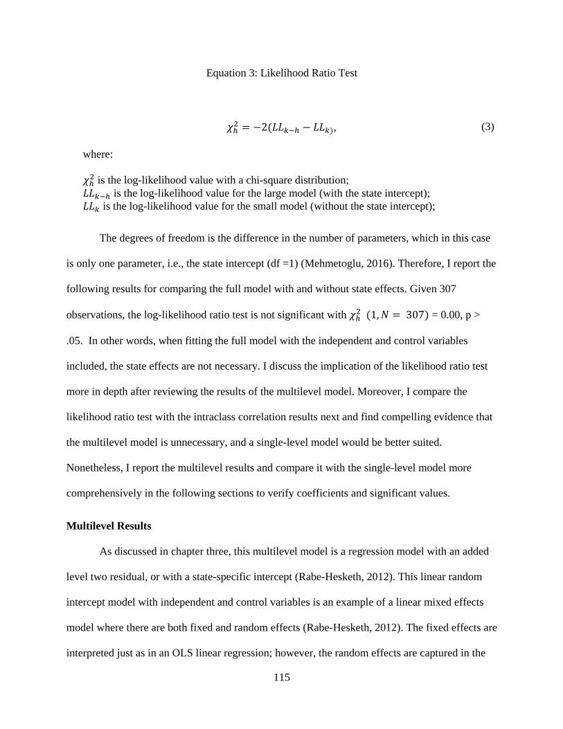
115
Equation 3: Likelihood Ratio Test
𝜒𝜒ℎ2 = −2(𝐿𝐿𝐿𝐿𝑘𝑘−ℎ − 𝐿𝐿𝐿𝐿𝑘𝑘),
(3)
where: 𝜒𝜒ℎ2 is the log-likelihood value with a chi-square distribution; 𝐿𝐿𝐿𝐿𝑘𝑘−ℎ is the log-likelihood value for the large model (with the state intercept); 𝐿𝐿𝐿𝐿𝑘𝑘 is the log-likelihood value for the small model (without the state intercept);
The degrees of freedom is the difference in the number of parameters, which in this case
is only one parameter, i.e., the state intercept (df =1) (Mehmetoglu, 2016). Therefore, I report the
following results for comparing the full model with and without state effects. Given 307
observations, the log-likelihood ratio test is not significant with 𝜒𝜒ℎ2 (1,𝑁𝑁 = 307) = 0.00, p >
.05. In other words, when fitting the full model with the independent and control variables
included, the state effects are not necessary. I discuss the implication of the likelihood ratio test
more in depth after reviewing the results of the multilevel model. Moreover, I compare the
likelihood ratio test with the intraclass correlation results next and find compelling evidence that
the multilevel model is unnecessary, and a single-level model would be better suited.
Nonetheless, I report the multilevel results and compare it with the single-level model more
comprehensively in the following sections to verify coefficients and significant values.
Multilevel Results
As discussed in chapter three, this multilevel model is a regression model with an added
level two residual, or with a state-specific intercept (Rabe-Hesketh, 2012). This linear random
intercept model with independent and control variables is an example of a linear mixed effects
model where there are both fixed and random effects (Rabe-Hesketh, 2012). The fixed effects are
interpreted just as in an OLS linear regression; however, the random effects are captured in the
116
state effects random intercept. Subsequently, the level 1 variance component represents the
variance within each state, whereas the level 2 variance component represents the variance
between each state (Mehmetoglu, 2016).
The voter turnout multilevel model is estimated with 23 states since county-level voter
turnout was not available for Alaska, albeit the initiative is permitted at the state-level. There are
307 observations included in estimating this model. Of the 307 observations, there are 23 states
with an average of 13.3 observations per state, with a minimum of 1 and maximum of 30
observations across all states. The mean county voter turnout (constant) measurement is .345 or
34.5 percent. The author tested for interaction effects between the county level initiative and
state voter registration rate, also called cross-level interaction effects since the terms are from
level 1 and level 2 of the model (Rabe-Hesketh, 2012). However, the interaction term of the
county initiative by state voter registration rate failed to produce any significant results. The
estimated level I (remaining estimated residual variance) not due to additive effects of states is
.003, and the level II (residual variance) between states is .000.
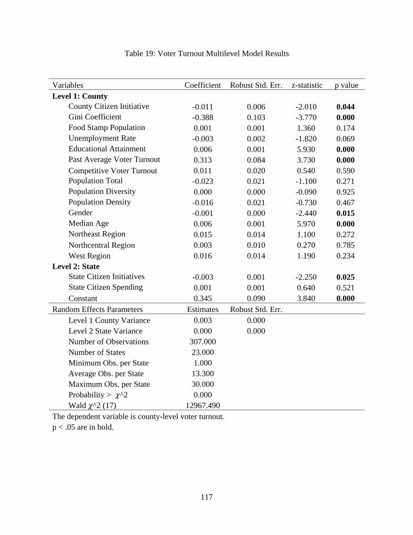
117
Table 19: Voter Turnout Multilevel Model Results
Variables Coefficient Robust Std. Err. z-statistic p value Level 1: County
County Citizen Initiative -0.011 0.006 -2.010 0.044 Gini Coefficient -0.388 0.103 -3.770 0.000 Food Stamp Population 0.001 0.001 1.360 0.174 Unemployment Rate -0.003 0.002 -1.820 0.069 Educational Attainment 0.006 0.001 5.930 0.000 Past Average Voter Turnout 0.313 0.084 3.730 0.000 Competitive Voter Turnout 0.011 0.020 0.540 0.590 Population Total -0.023 0.021 -1.100 0.271 Population Diversity 0.000 0.000 -0.090 0.925 Population Density -0.016 0.021 -0.730 0.467 Gender -0.001 0.000 -2.440 0.015 Median Age 0.006 0.001 5.970 0.000 Northeast Region 0.015 0.014 1.100 0.272 Northcentral Region 0.003 0.010 0.270 0.785 West Region 0.016 0.014 1.190 0.234
Level 2: State State Citizen Initiatives -0.003 0.001 -2.250 0.025 State Citizen Spending 0.001 0.001 0.640 0.521 Constant 0.345 0.090 3.840 0.000
Random Effects Parameters Estimates Robust Std. Err. Level 1 County Variance 0.003 0.000 Level 2 State Variance 0.000 0.000 Number of Observations 307.000 Number of States 23.000 Minimum Obs. per State 1.000 Average Obs. per State 13.300 Maximum Obs. per State 30.000 Probability > 𝜒𝜒^2 0.000 Wald 𝜒𝜒^2 (17) 12967.490
The dependent variable is county-level voter turnout. p < .05 are in bold.

118
Intraclass Correlation
On closer inspection, the level 1 and level 2 variance components are negligible. To
investigate these results, I calculate the amount of level 2 variance explained in the MLM by
calculating the intraclass correlation coefficient, i.e., also known as the variance partition
coefficient (Mehmetoglu, 2016). The intraclass correlation coefficient represents the proportion
of total variability in the outcome that is attributable to the second level, which can be derived by
using the equation below.
Equation 4: Intraclass Correlation Coefficient
var (εj,t)
var (εi,t) + (εj,t)
(4)
where:
εi,t is the level 1 variance component (within group variance) and εj,t is the level 2 variance
component (between group variance).
In multilevel regression, the standard errors of the state variables are estimated based on
the N at the state-level (Mehmetoglu, 2016). If the state-level intraclass correlation coefficient
(ICC) is so low that it is equal to zero, no group differences exist for the variables of interest
(Kreft & Leeuw, 1998; Winneg et al., 2013). I provide the ICC model results in table 20 as a
reference to contrast the differences between the null model (no predictors) and the full model.
As described by Mehmetoglu (2016), the results for the null model with no predictors included
indicates in ICC of 13.2 percent that is explained by the level 2 random state intercept. Robson &
David (2015) advocate for a somewhat flexible guideline around 10 percent as being indicative
of a nontrivial ICC. Moreover, the intraclass correlation is negligible after fitting the full model
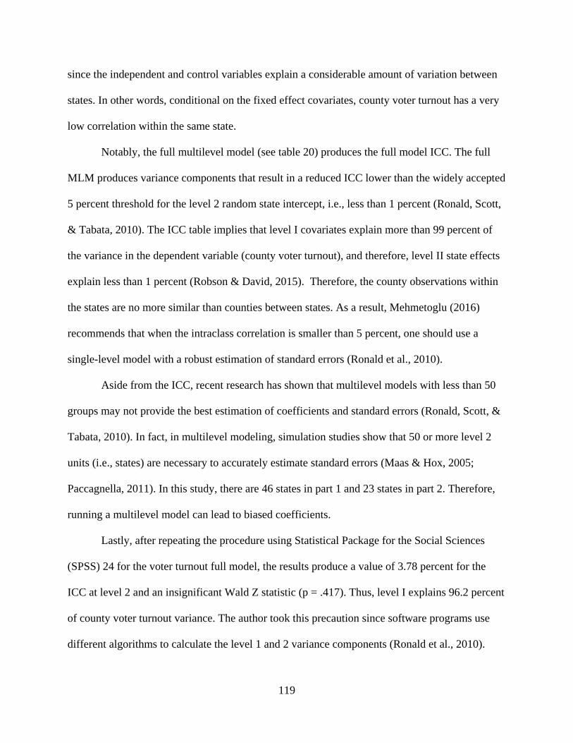
119
since the independent and control variables explain a considerable amount of variation between
states. In other words, conditional on the fixed effect covariates, county voter turnout has a very
low correlation within the same state.
Notably, the full multilevel model (see table 20) produces the full model ICC. The full
MLM produces variance components that result in a reduced ICC lower than the widely accepted
5 percent threshold for the level 2 random state intercept, i.e., less than 1 percent (Ronald, Scott,
& Tabata, 2010). The ICC table implies that level I covariates explain more than 99 percent of
the variance in the dependent variable (county voter turnout), and therefore, level II state effects
explain less than 1 percent (Robson & David, 2015). Therefore, the county observations within
the states are no more similar than counties between states. As a result, Mehmetoglu (2016)
recommends that when the intraclass correlation is smaller than 5 percent, one should use a
single-level model with a robust estimation of standard errors (Ronald et al., 2010).
Aside from the ICC, recent research has shown that multilevel models with less than 50
groups may not provide the best estimation of coefficients and standard errors (Ronald, Scott, &
Tabata, 2010). In fact, in multilevel modeling, simulation studies show that 50 or more level 2
units (i.e., states) are necessary to accurately estimate standard errors (Maas & Hox, 2005;
Paccagnella, 2011). In this study, there are 46 states in part 1 and 23 states in part 2. Therefore,
running a multilevel model can lead to biased coefficients.
Lastly, after repeating the procedure using Statistical Package for the Social Sciences
(SPSS) 24 for the voter turnout full model, the results produce a value of 3.78 percent for the
ICC at level 2 and an insignificant Wald Z statistic (p = .417). Thus, level I explains 96.2 percent
of county voter turnout variance. The author took this precaution since software programs use
different algorithms to calculate the level 1 and 2 variance components (Ronald et al., 2010).

120
Since the likelihood ratio test and intraclass correlation coefficient show that the level 2
random state intercept explains very little of the variance in county-level voter turnout, using the
single-level model will avoid an ecological fallacy i.e., this would be the case if the level 2 ICC
for the full MLM was higher than 5 percent as well. An ecological fallacy is failing to
acknowledge the potential variability present among individuals within groups, which can bias
estimates (Ronald, Scott, & Tabata, 2010). Consequently, the log-likelihood ratio test agrees
with the intraclass correlation results supporting the notion that a single-level model is better
suited to predict county voter turnout in this context. In turn, after fitting the full models, the
likelihood ratio test and intraclass correlation coefficients show that there is hardly any shared
context of dependency among observations between each state once accounting for independent
and control variables (Mehmetoglu, 2016). This exercise also reinforces the proper notion of
model specification to estimate the overall voter turnout model effects.
Table 20: Intraclass Correlation Coefficients
Model Variance Component ICC Std. 95% lower 95% upper Null Model Level 2 0.132 0.055 0.056 0.280 Full Model Level 2 0.001 0.000 0.001 0.001 Notes. ICC = Intraclass Correlation Coefficient
AIC and BIC Test
I perform one final test to compare model fit between the multilevel and single-level
models by using the Akaike’s information criterion (AIC) and Bayesian information criterion
(BIC) tests (see table 21). The AIC and BIC are tested to compare two information criteria
between models. Unlike the likelihood – ratio tests, and similar testing procedures, the models do
not need to be nested to compare the information criteria (Rabe-Hesketh, 2012; Stata, 2015). In
general, “smaller is better’, given two models, the one with the smaller AIC and BIC indicates a

121
better fitting model (Stata, 2015). As noted in the voter turnout AIC/BIC table, both the AIC and
BIC are smaller for the single level model when compared to the multilevel model.
In fact, regardless of the AIC and BIC negative values for both tests, the single-level
model has a smaller AIC by 4 units, and a smaller BIC by 11.45 units. Both the AIC and BIC
produce results that agree with each other, which is not always the case. Thus, this is one
additional test that indicates the single-level model is better suited to fit the data as opposed to
the multilevel model.
Table 21: Voter Turnout AIC and BIC Results
Model Obs. ll(null) ll(model) df AIC BIC Multilevel Model 307.00 473.65 19.00 -909.30 -838.49 Single-level Model 307.00 285.14 473.65 17.00 -913.30 -849.94 Notes. Results compare Akaike's information criterion (AIC) Bayesian information criterion (BIC); ll = log likelihood
Given the results of the likelihood ratio test, the ICC, and AIC/BIC test, I rerun the voter
turnout model using the rreg command in Stata. This procedure is useful because it performs a
robust estimation of standard errors while first performing an initial screening based on Cook’s
distance > 1 to eliminate gross outliers before calculating coefficients (Adkins & Hill, 2011). I
provide the single-level model results and interpretations in the next section.
Single-Level Model 1 Interpretations
The single-level robust regression in model one produces an F-statistic of 103.36,
reflecting that the overall model of the independent variables is useful in predicting the mean
county-level voter turnout. The mean voter turnout is 24 percent, as reflected by the constant
(intercept) term in the model output. The rreg procedure does not report an R-square value;
however, a standard regression using the same model reports an R-square value of .707. In turn,
122
the independent and control variables in this model explain about 70 percent of the variance in
county level voter turnout. According to Mehmetoglu (2016), the relatively high value of the R-
square value confirms that the model fits the data well.
I now turn to the interpretation of the slope coefficients for each hypothesis (see table
20). Hypothesis 6 testing the relationship between the county initiative and voter turnout is
significant; however, the coefficient is in the negative direction as opposed to the positive
direction as originally expected. Accordingly, the coefficient is -.0103 at p < .05, reflecting that
counties with the initiative available were associated with 1.03 percent less voter turnout than
counties without the initiative. I discuss the implication of hypothesis 6 more in-depth with
hypothesis 11 below as both measure the citizen initiative effects at the county and state levels.
Hypothesis 7 is significant in the expected direction for the Gini coefficient. Since the
Gini coefficient is measured on a scale from 0 to 1, a .1 change in the Gini coefficient causes -
.22% less county voter turnout. In other words, more income inequality causes lower voter
turnout. Hypothesis 8 regarding the poverty measure for food stamp population and hypothesis 9
regarding the unemployment rate both failed to show any significant associations with county
level voter turnout. Hypothesis 10 measuring the association between education and county level
voter turnout is significant, with a coefficient of .004 and p-value < .05. Hypothesis 10 is
modeled as the percent of the population 25 years and older with a bachelor’s degree. Therefore,
a 1 percent increase in an educated population relates to a .4% increase in expected county voter
turnout.
Hypothesis 11 measuring the association between the number of state citizen initiatives
on the ballot and county-level voter turnout is significant with a coefficient of -.003 and a p value
of < .05. In this case, for each additional citizen initiative on the ballot at the state level, voter
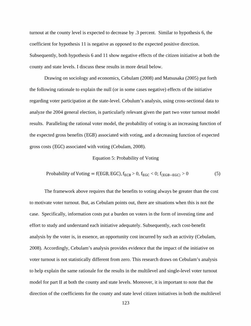
123
turnout at the county level is expected to decrease by .3 percent. Similar to hypothesis 6, the
coefficient for hypothesis 11 is negative as opposed to the expected positive direction.
Subsequently, both hypothesis 6 and 11 show negative effects of the citizen initiative at both the
county and state levels. I discuss these results in more detail below.
Drawing on sociology and economics, Cebulam (2008) and Matsusaka (2005) put forth
the following rationale to explain the null (or in some cases negative) effects of the initiative
regarding voter participation at the state-level. Cebulum’s analysis, using cross-sectional data to
analyze the 2004 general election, is particularly relevant given the part two voter turnout model
results. Paralleling the rational voter model, the probability of voting is an increasing function of
the expected gross benefits (EGB) associated with voting, and a decreasing function of expected
gross costs (EGC) associated with voting (Cebulam, 2008).
Equation 5: Probability of Voting
Probability of Voting = f(EGB, EGC), fECB > 0, fEGC < 0; f(EGB−EGC) > 0
(5)
The framework above requires that the benefits to voting always be greater than the cost
to motivate voter turnout. But, as Cebulam points out, there are situations when this is not the
case. Specifically, information costs put a burden on voters in the form of investing time and
effort to study and understand each initiative adequately. Subsequently, each cost-benefit
analysis by the voter is, in essence, an opportunity cost incurred by such an activity (Cebulam,
2008). Accordingly, Cebulam’s analysis provides evidence that the impact of the initiative on
voter turnout is not statistically different from zero. This research draws on Cebulam’s analysis
to help explain the same rationale for the results in the multilevel and single-level voter turnout
model for part II at both the county and state levels. Moreover, it is important to note that the
direction of the coefficients for the county and state level citizen initiatives in both the multilevel
124
and single-level models were both signed negative. Along these lines, Fountaine (1988) notes
that the “educative effect” for increasing political participation is limited since voters can be
bombarded with political advertising designed to manipulate opinions by appealing to voters’
emotions rather than provide useful information on issues (Zimmerman, 2015). Similarly, Jacobs
(1997) reported that only 5 percent of interviewees in California understood initiative
propositions (Zimmerman, 2015). Finally, hypothesis 12 measuring the per capita effects of
spending (for and against) on state-level citizen initiative campaigns show, on average, no
significant effect on county-level voter turnout.
Control Variables Interpretations
The control variables show some expected but noteworthy predictive power on county
level voter turnout. One of the most important control variables, average voter turnout is
significant with a coefficient of .575 and a p value < .05. Since the average voter turnout is a
percentage, the coefficient shows that for each 1 percent increase in past average voter turnout,
the 2016 turnout can expect an increase by .575 percent. As discussed in chapter two, this control
variable has theoretical value to isolate the effect of the main hypotheses, and in effect provide
more accurate estimations. The theoretical nature of controlling for competitive elections shows
no significant impact on explaining voter turnout at the county level.
The control variable measuring total populations is scaled by 10 million. While not
significant, for each increase in 1 million people by county, it is expected that county voter
turnout would increase by .1 percent. Recall that population diversity is the probability that two
individuals chosen at random would be of different races between 2012 and 2016. Therefore, an
increase in one probability unit equates to a small (-.1 percent) but significant decrease in voter
turnout.

125
Changes in population density showed no significant association with predicting voter
turnout. Gender is an estimated ratio of males to females; therefore, a significant coefficient of -
.1 percent reflects that women are more inclined to vote than males. As expected, people are
more inclined to vote as they get older given the significant positive coefficient of .3 percent.
The regions are all insignificant except for the northcentral region, which has a -1.2 percent
coefficient. Therefore, voters residing in this region are expected to turnout less as opposed to
voters in the south region (reference group) of the United States.
Single-Level Model 2 Interpretations
The researcher repeats the voter turnout analysis in model two but removes California to
examine any potential outlier influence attributable from the state’s exceptionally active citizen
initiative usage. The rationale is the same as discussed in part one. Essentially, the state of
California has one of the most active electorates for citizen initiatives (Goebel, 2002). Therefore,
by removing California, the researcher examines the results for outliers that may have caused
directional changes in the coefficients. Notably, the researcher expects that removing California
will substantially reduce the sample power in picking up significant results (Rabe-Hesketh,
2012). Subsequently, in this case, model two contains 22 states and 289 counties. Nonetheless,
the results for model two reveal important considerations. Notably, the direction of county
citizen initiative is negative at -.008 and the state citizen initiative is negative at -.002. While
both coefficients are insignificant, the signs are both in the negative direction. Therefore, these
results also largely support hypotheses 6 and 11 showing that citizen initiatives do not always
increase voter turnout.

126
Single-Level Results
Table 22: Voter Turnout Single-Level Model Results
Model 1 Variables Coefficient Robust Std. Err. t-statistic p value Political Institution
Citizen Initiative -0.010 0.005 -2.220 0.027 Socioeconomic
Gini Coefficient -0.218 0.079 -2.770 0.006 Food Stamp Population 0.001 0.001 1.580 0.115 Unemployment Rate -0.001 0.001 -1.210 0.228 Educational Attainment 0.004 0.001 6.970 0.000
Controls Past Average Voter Turnout 0.575 0.031 18.300 0.000 Competitive Voter Turnout -0.003 0.013 -0.210 0.837 Population Total 0.011 0.046 0.240 0.814 Population Diversity -0.001 0.000 -3.740 0.000 Population Density 0.003 0.027 0.120 0.901 Gender -0.001 0.000 -4.750 0.000 Median Age 0.003 0.001 6.830 0.000 Northeast Region -0.009 0.015 -0.600 0.551 Northcentral Region -0.012 0.006 -2.010 0.045 West Region 0.000 0.008 -0.030 0.976
State Variables State Citizen Measures -0.003 0.001 -2.510 0.013 State Citizen Spending 0.001 0.001 1.640 0.102
Constant 0.240 0.045 5.300 0.000 F (17, 289) 103.360 Prob > F 0.000 Number of Observations 307.000 Notes. The dependent variable is county-level voter turnout. p < .05 are in bold.

127
Table 23: Voter Turnout Single-Level Model 2 Results
Model 2 Variables Coefficient Robust Std. Err. t-statistic p value Political Institution
Citizen Initiative -0.008 0.005 -1.740 0.082 Socioeconomic
Gini Coefficient -0.207 0.082 -2.540 0.012 Food Stamp Population 0.001 0.001 1.400 0.164 Unemployment Rate -0.002 0.001 -1.610 0.109 Educational Attainment 0.004 0.001 6.050 0.000
Controls Past Average Voter Turnout 0.591 0.033 18.030 0.000 Competitive Voter Turnout 0.009 0.014 0.680 0.495 Population Total 1.456 0.333 4.380 0.000 Population Diversity -0.001 0.000 -3.230 0.001 Population Density -0.131 0.046 -2.850 0.005 Gender -0.001 0.000 -3.800 0.000 Median Age 0.004 0.001 7.310 0.000 Northeast Region -0.004 0.016 -0.270 0.786 Northcentral Region -0.010 0.006 -1.640 0.103 West Region -0.001 0.008 -0.090 0.925
State Variables State Citizen Measures -0.002 0.002 -0.870 0.384 State Citizen Spending 0.001 0.001 0.650 0.518
Constant 0.193 0.047 4.130 0.000 F (17, 271) 92.260 Prob > F 0.000 Number of Observations 289.000 Notes. The dependent variable is county-level voter turnout. p < .05 are in bold.

128
Initiative Predictions
A useful procedure after estimating the regression model is to use the coefficients to
calculate the expected change in the outcome variable at different values of an independent
variable. In this case, the primary independent variables of interest are the availability of the
county-level initiative and the number of state level initiatives in the 2016 election. While
holding all independent variables constant (at their mean values), I use the margins and margins
plot commands to first estimate changes in mean county voter turnout for given values of the
county initiative, at either zero or one.
After the county-level citizen initiative estimation, I repeat the procedure for county level
voter turnout for given values of the number of state level citizen initiatives, at values between 0
and 14. Notably, I use the 0 thru 14 range of state level citizen initiatives since these are the “in-
sample” values recorded in the 2016 election. I plot these changes based on the final single-level
regression equation estimated in table 11.
The margins command is very useful since it calculates the 95 percent confidence intervals
around the predicted values (Mehmetoglu, 2016). The results for the county initiative show that a
county without the citizen initiative has a predicted voter turnout of 57.5 percent, whereas a
county with the citizen initiative has a predicted voter turnout of 56.5 percent. The 1 percent
negative difference for counties that have the initiative is noticeable given the negative slope in
figure 7.
The results for the state initiative show that a county with one state initiative on the ballot
has an expected voter turnout of 57 percent, whereas a county with 14 state initiatives on the
ballot has an expected voter turnout of 54 percent. Similar to the county initiative, the 3 percent
negative difference for voter turnout is noticeable given the negative slope in figure 8. Finally, I
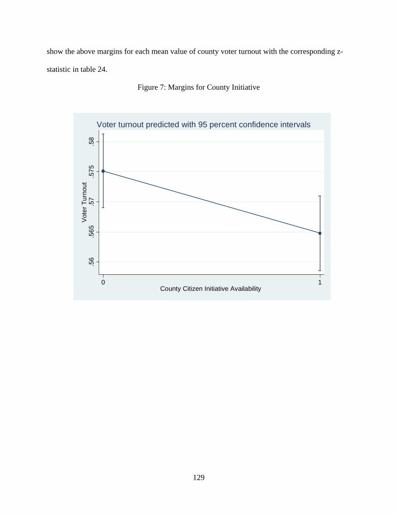
129
show the above margins for each mean value of county voter turnout with the corresponding z-
statistic in table 24.
Figure 7: Margins for County Initiative
.56
.565
.57
.575
.58
Vote
r Tur
nout
0 1County Citizen Initiative Availability
Voter turnout predicted with 95 percent confidence intervals
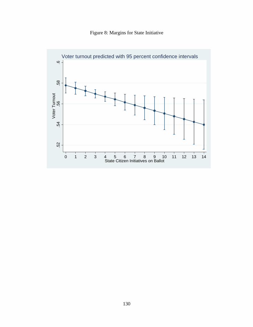
130
Figure 8: Margins for State Initiative
.52
.54
.56
.58
.6Vo
ter T
urno
ut
0 1 2 3 4 5 6 7 8 9 10 11 12 13 14State Citizen Initiatives on Ballot
Voter turnout predicted with 95 percent confidence intervals

131
Table 24: County and State Predictive Margins
County Initiative Margins Std. Error Z P > z Lower 95% Upper 95% 0 0.575 0.003 184.080 0.000 0.569 0.581 1 0.565 0.003 178.830 0.000 0.559 0.571
Notes. Margins based on 307 observations.
State Initiative Margins Std. Error Z P > z Lower 95% Upper 95% 0 0.578 0.004 151.950 0.000 0.570 0.585 1 0.575 0.003 194.220 0.000 0.569 0.581 2 0.573 0.002 245.710 0.000 0.568 0.577 3 0.570 0.002 270.500 0.000 0.566 0.574 4 0.567 0.002 235.530 0.000 0.562 0.572 5 0.564 0.003 183.030 0.000 0.558 0.570 6 0.562 0.004 142.330 0.000 0.554 0.569 7 0.559 0.005 114.120 0.000 0.549 0.569 8 0.556 0.006 94.350 0.000 0.545 0.568 9 0.553 0.007 80.000 0.000 0.540 0.567 10 0.551 0.008 69.200 0.000 0.535 0.566 11 0.548 0.009 60.830 0.000 0.530 0.566 12 0.545 0.010 54.170 0.000 0.526 0.565 13 0.543 0.011 48.760 0.000 0.521 0.564 14 0.540 0.012 44.270 0.000 0.516 0.564
Notes. Margins based on 307 observations.
Summary
In summary, chapter four has presented model diagnostics with several different tests for
model specification, the results with interpretations, and finally graphs to show predictive
margins and articulate findings. The logistic analysis presented various perspectives to answer
the government structure hypotheses for part one, whereas the multilevel and single-level models
were both used to address the voter turnout hypotheses for part two. In chapter five, the author
concludes this dissertation by reviewing lessons learned and implications for future policy.

132
Chapter 5: Conclusions
Lessons Learned
Part I
The government structure model examines the probability of the county-level initiative
for several common forms of county government in the United States. The model finds a strong
association between the commission and council-elected governments and the availability of the
initiative relative to the council-manager and council-administrator governments. The
commission and council elected governments emphasize elected representatives more so than the
council-manager and council-administrator governments (Menzel, 1996). These findings have
three implications.
First, the findings support the notion that elected representatives represent the attitudes
and interest of citizens at the county-level. As discussed in chapter two, public opinion polls
have shown that citizens prefer to have the initiative available, and both the commission and
council-elected governments emphasize elected representatives (Childers & Binder, 2012a;
Dalton et al., 2001). This rationale is also given consideration since county government officials
act much like a governor by carrying out executive functions as an elected official (H.
Duncombe, 2007). Commissioners, council-elected representatives, and governors all share the
responsibility of representing the attitudes and interest of citizens as elected officials.

133
Second, county governments take on legislative functions such as establishing policy,
enacting ordinances, adopting revenue measures, appropriating money, and making political
appointments (Frederickson, 2003). Given these legislative responsibilities, Dubois & Feeney
(1998) point out that the initiative regulates excessive campaign spending, gerrymandering,
unfair committee assignments, logrolling, pork-barrel legislation, and inept representatives.
Dubois & Feeney (1998) also note that drafters craft initiatives with more care than legislative
bills since they cannot be changed, initiatives do not create a tyranny of the majority since they
are subject to judicial review, and voters do not always selfishly vote for their pocketbooks.
Given these arguments, it is evident that the initiative works as a safeguard mechanism for bad
behavior by legislators (Matsusaka, 2005). Therefore, responsible commissioners may enact the
initiative to work as a check on future administrations to prevent political malfeasance.
Third, a tangential argument that leads to the same outcome is that county commissioners
may favor the initiative since it removes responsibility away from their own policymaking
process by engaging public opinion. Many tax limitation rules adopted through direct democracy
continue to shape fiscal policy in states like California and Oregon (Bowler et al., 1998).
However, voters are not necessarily against funding programs (Bowler et al., 1998). For instance,
proposition 98 was passed by voters in California to guarantee a minimum level of funding for
public schools and community colleges that keeps pace with the personal income of Californians
(Bowler et al., 1998). Extending Bowler’s argument, it is conceivable that certain constituents
could attack a county commissioner for raising taxes for the same funding proposition. But, by
allowing the public to weigh in on the matter, the county commissioner can shirk the
responsibility by allowing citizens to initiate legislation and vote on the issue. Subsequently, the
funding for a social good is successful, and the county commissioner does not have to deal with
134
the political backlash from constituents that may not have supported the tax increase in the first
place.
The government structure model also reveals important implications showing that
counties afforded the home rule authority are more likely associated with having the initiative.
As Menzel (1996) shows, home rule authority allows counties the powers to govern themselves
more effectively. In this case, the evidence shows that counties with such authority have used it
to meet the demands of the citizenry by enacting the initiative. Aside from this, higher per capita
income is more likely associated with the initiative, whereas higher education is less likely
associated with the initiative. In this case, the effects of higher per capita income were very mild.
However, as discussed in chapter four, higher educational attainment has a more significant
effect on the availability of the initiative. In this regard, highly educated policymakers elected
from the citizenry understand the value of the initiative and may want to prevent handing over
power to citizens (Dubois & Feeney, 1998). As Bowler (1998) and Dubois & Feeney (1998)
discuss at length, one of the main points of the initiative is to give citizens the power to initiate
legislation when legislators fail to act in the citizens’ best interest.
Part II
The voter turnout model uses a multilevel design implemented by Knotts & Haspel
(2006) to compare signs and coefficients with the single-level design used by Arbour & Hayes
(2005). Following Linimon & Joslyn (2002), the voter turnout model capitalizes on the
theoretical value of using past average turnout data in three presidential elections as a control
variable. Aside from the past average voter turnout, the models control for numerous other
factors at the county-level. After carrying out numerous model specification analyses that test for
135
heteroscedasticity, multicollinearity, omitted variable bias, and goodness of fit, I draw the
following conclusions.
The multilevel and single level regression analyses both indicate that the initiative at the
county and state levels contribute to a negative and significant contribution to county voter
turnout. Mehmetoglu (2016) recommends using different versions of the regression to address
the robustness of the findings. From this perspective, both the multilevel and single-level model
results agree with each other in that the county and state initiatives negatively contribute to voter
turnout. At the very least, these analyses fall in line with Cebulam's (2008) study, which
concluded that the information cost required of citizens could outweigh the benefits of voting.
Therefore, the result of the information cost can ultimately hinder voter participation.
Additionally, this study contributes to the literature by examining the effects of the
county initiative on a national scale since prominent studies have focused on state initiatives,
e.g., see Tolbert et al. (2009). This study also contributes to the literature by showing that higher
income inequality has a negative impact on voter turnout at the county-level. Finally, a highly
educated citizenry proves to be a positive and significant factor for increasing political
participation within counties.
Limitations
All research designs have limitations. Granted, the author acknowledges an aspect of the
county-level initiative that was of particular interest in part two of the voter turnout model.
Specifically, as discussed in chapter two, the use of the county level initiative on the 2016 ballot
was not available. However, even though the use of the county ballots on the national level was
unavailable, over 800 county level initiatives were used in California alone (Graves, 2012).
Therefore, assessing the availability of the county initiative likely picked up a great deal of the

136
use of the county initiative on the ballot. Then, I produce additional analyses for both part one
and part two while excluding California. The latter results provide consistent evidence in favor
of the citizen initiative conclusions. Nonetheless, future research may want to conduct a single-
state case study on the use of the county initiative in California alone, similar to Arbour & Hayes
(2005) but using the voter turnout model in this study as a basis for investigation. Additional
research can examine voter turnout within the context of hot button public policy issues as well.
For example, extending the research of Burnett & Mccubbins (2014) to focus on whether the
legalization of marijuana or same-sex marriage has an impact on county-level voter turnout can
provide useful results for this research area.
Lastly, the researcher acknowledges that political participation is typically higher during
presidential election years (Winneg, Hardy, & Hall Jamieson, 2013). Therefore, it will be
worthwhile in the future to investigate the impact of county initiatives during midterm elections
as well as presidential elections. In fact, similar to Tolbert, Grummel, & Smith (2009), but
emphasizing county initiatives on midterm elections. More importantly, it will be important to
examine whether county initiatives have a positive or negative impact on political participation
during midterm elections.
Future Policy
As discussed by Salant (2007), the governance of American counties are moving away
from the commission structure and toward reformed governments that include the council-
elected, council manager, and council-administrator governments. Therefore, based on the
evidence, the government structure model offers two primary implications for future policy.
First, commission governments represent the most democratic form of county government given
that all commissioners serve on the basis of competitive democratic elections. This study shows
137
that the commission governments have a high association with the citizen initiative. Moving
away from the commission government may result in less favorable odds of having the citizen
initiative available.
Second, and equally important, the author realizes that momentum has been building
toward reformed governments that take advantage of an executive that unifies the administration
of county services, e.g., executives that handle budgeting, adopting ordinances, and hiring/firing
department heads (Choi et al., 2010; DeSantis, 2007; Menzel & Thomas, 1996). Accordingly, the
evidence in the government structure model shows that there is a modest association between the
elected government and the initiative. Considering this evidence, policymakers and citizens alike
can consider the council-elected structure as a government that combines competitively elected
executives with a governing board that can respond more effectively to citizen demands. As
discussed in chapter two, if the elected executive in the council government performs poorly or
does not respond adequately to community challenges, then that representative will be voted out
of office. The distinction between the council-elected and other reformed governments is that it
is the citizens that can determine voting the executive out of office, whereas the other reformed
governments, swayed by special interests, may keep the executive in place.
In part two, the voter turnout model revealed important evidence regarding the effect of
the initiative on voter turnout at the county and state levels. There is a large body of evidence to
show the benefits of the initiative that broadly concerns the citizenry. A brief list includes
limiting property taxes, increasing the minimum wage, legalizing marijuana and gambling,
addressing gun control, and funding stem cell research (Matsusaka, 2005). These hot button
issues typically drive policy debates with political fervor. Nonetheless, as Cebulam (2008) points
out, each of these issues requires voters to take the time to understand and vote on the issues. The

138
impact is an information cost that may outweigh the benefit of voting. When subjected to the
rigor of numerous model specification tests (e.g., lack of specification tests in Tolbert et al.,
2009), well-grounded control variables, and sensitivity analyses, the voter turnout model
suggests that citizen initiatives do not always increase voter turnout. The strain on political
participation can have ripple effects that impact policymakers, special-interest organizations, and
candidates for office. More specifically, policymakers should consider the impact of enacting the
initiative at the county and/or state level, special-interest groups may experience diminishing
returns after a certain level of messaging during initiative campaigns, and candidates may either
experience an advantage or disadvantage when running for office during initiative campaigns.
Future research should further investigate the causality between the initiative and voter turnout,
especially with granular units of analysis such as the individual or county, as opposed to the vast
majority of the direct democracy research produced at the state-level.

139
Appendix A: MLM and Single-Level Model Comparison
Given the model specifications, there is little difference between the multilevel and
single-level model coefficients and significant values for primary independent variables of
interest. Nonetheless, as discussed in chapter four, there is solid evidence that a single-level
model is better suited to fit the data for the voter turnout model specifications. I provide the
following interpretation for table 25 as a reference.
Based on the results, the multilevel model has seven variables that are significant,
whereas the single-level model has nine variables that are significant. The primary hypotheses of
the county and state-level citizen initiatives are both signed significantly negative in both the
multilevel model and single level model results. The northcentral region is significant in the
single-level model, as opposed to the insignificant value in the multilevel model. The single
level model shows a significant value for the population diversity at -.001 (p < .05), whereas it is
insignificant in the multilevel model. In other words, in the single level model, more diversity is
associated with lower county-level voter turnout.

140
Table 25: MLM and Single-Level Model Comparison Results
Model MLM SLM Variables Coefficient p value Coefficient p value
Citizen Initiative -0.011 0.044 -0.010 0.027 Gini Coefficient -0.388 0.000 -0.218 0.006 Food Stamp Population 0.001 0.174 0.001 0.115 Unemployment Rate -0.003 0.069 -0.001 0.228 Educational Attainment 0.006 0.000 0.004 0.000 Past Average Turnout 0.313 0.000 0.575 0.000 Competitive Turnout 0.011 0.590 -0.003 0.837 Population Total -0.023 0.271 0.011 0.814 Population Diversity 0.000 0.925 -0.001 0.000 Population Density -0.016 0.467 0.003 0.901 Gender -0.001 0.015 -0.001 0.000 Median Age 0.006 0.000 0.003 0.000 Northeast Region 0.015 0.272 -0.009 0.551 Northcentral Region 0.003 0.785 -0.012 0.045 West Region 0.016 0.234 0.000 0.976 State Citizen Measures -0.003 0.025 -0.003 0.013 State Citizen Spending 0.001 0.521 0.001 0.102
Constant 0.345 0.000 0.240 0.000 Notes. The dependent variable is county-level voter turnout; p < .05 are in bold. MLM = multilevel model; SLM = single-level model.

141
References
Acock, A. (2013). Discovering Structural Equation Modeling Using Stata. Stata Press.
Adkins, L., & Hill, C. (2011). Using Stata for Principles of Econometrics. Hoboken: Wiley.
Ammons, D. N., & Newell, C. (1988). “City managers don’t make policy:” A lie; let’s face it.
National Civic Review, 77(2), 124–132.
Arbour, B. K., & Hayes, D. (2005). Voter turnout in the California recall: Where did the increase
come from? American Politics Research, 33(2), 187–215.
Arceneaux, K. (2002). Direct Democracy and the Link between Public Opinion and State
Abortion Policy. State Politics and Policy Quarterly, 2(4), 372–387.
Bali, V. A. (2008). The Passage of Education Citizen Initiatives. Educational Policy, 22(3), 422–
456.
Becker, R., & Antic, G. (2016). Statistical control in correlational studies: 10 essential
recommendations for organizational researchers. Journal of Organizational Behavior,
17(2), 1–20.
Benton, E. (2002). County Service Delivery: Does Government Structure Matter? Public
Administration Review, 62(4), 471–479.
Benton, E. (2005). An Assessment of Research on American Counties. Public Administration
Review, 65(4), 462–474.
Benton, J. E. (2003). The Impact of Structural Reform on County Government Service Provision.
Social Science Quarterly, 84(4), 858–874.
Berman, D. (1993). County Governments in an Era of Change. Greenwood Press.
Bernisky, A., & Lenza, G. (2011). Education and Political Participation: Exploring the Causal.
Political Behavior, 18(2), 197–206.

142
Boehmke, F. J. (2005). Sources of Variation in the Frequency of Statewide Initiatives: The Role
of Interest Group Populations. Political Research Quarterly, 58(1989), 565–575.
Bollen, K. A., & Jackman, R. W. (1985). Political Democracy and the Size Distribution of
Income. Ciological Review, 1985, 50(4), 438–457.
Bowler, S., & Donovan, T. (2002). Democracy, Institutions and Attitudes about Citizen
Influence on Government. Cambridge University Press, 32(2), 371–390.
Bowler, S., Donovan, T., & Tolbert, C. (1998). Citizens as Legislators: Direct Democracy in the
Unites States. Ohio State University Press.
Bowler, S., Nicholson, S. P., & Segura, G. M. (2006). Earthquakes and aftershocks; race, direct
democracy, and partisan change. American Journal of Political Science, 50(1), 146–159.
Bunch, J. (2014). Does Local Autonomy Enhance Representation? The Influence of Home Rule
on County Expenditures. State and Local Government Review, 46(2), 106–117.
Burmila, E. M. (2017). Voter Turnout, Felon Disenfranchisement and Partisan Outcomes in
Presidential Elections, 1988–2012. Social Justice Research, 30(1), 72–88.
Burnett, C. M., & Mccubbins, M. D. (2014). Sex and the ballot box: Perception of ballot
measures regarding same-sex marriage and abortion in California. Journal of Public Policy,
34(1), 3–33. http://doi.org/10.1017/S0143814X13000226
Burnett, C. M., & Parry, J. A. (2014). Gubernatorial endorsements and ballot measure approval.
State Politics and Policy Quarterly, 14(2), 178–195.
Campbell, D., & Kenney, D. (1999). Primer on Regression Artifacts. New York: St. Martin’s
Press.
Campbell, R. (2007). City-County Consolidation: Learning from Failure. In Form of Local
Government. McFarland.

143
Carpenter, M. A., Geletkancz, M. A., & Sanders, W. G. (2004). Upper echelons research
revisited: Antecedents, elements, and consequences of top management team composition.
Journal of Management, 30(6), 749–778.
Carroll, D. A., & Goodman, C. B. (2011). The Effects of Assessment Quality on Revenue
Volatility. Public Budgeting and Finance, 31(1), 76–94.
Carswell, D. (2005). Direct Democracy: An Agenda for a New Model Party. Direct Democracy.
Cebulam, R. (2008). Does Direct Democracy Increase Voter Turnout? American Journal of
Economics and Sociology.
Childers, M., & Binder, M. (2012a). Engaged by the initiative? How the use of citizen initiatives
increases voter turnout. Political Research Quarterly, 65(1), 93–103.
Childers, M., & Binder, M. (2012b). Engaged by the Initiative? How the Use of Citizen
Initiatives Increases Voter Turnout. Political Research Quarterly, 65(1), 93–103.
Choi, S. O., Bae, S.-S., Kwon, S.-W., & Feiock, R. (2010). County Limits. The American Review
of Public, 29–45.
Coan, T. G., & Holman, M. R. (2008). Voting green. Social Science Quarterly, 89(5), 1121–
1135.
Collingwood, L. (2012). Levels of Education and Support for Direct Democracy. American
Politics Research, 40(4), 571–602.
Coombs, C. K., Sarafoglou, N., & Crosby, W. (2012). Property Taxation, Capitalization, and the
Economic Implications of Raising Property Taxes. International Advances in Economic
Research, 18(2), 151–161.
Coser, L. (1956). The Function of Social Conflict. New York: Free Press.
Dalton, R. J., Bürklin, B., & Drummond, A. (2001). Public Opinion and Direct Democracy.

144
Journal of Democracy, 12(4), 141–153.
Damore, D. F., Bowler, S., & Nicholson, S. P. (2012). Agenda setting by direct democracy:
Comparing the initiative and the referendum. State Politics and Policy Quarterly, 12(4),
367–393.
Delabbio, D. J., & Zeemering, E. S. (2013). Public Entrepreneurship and Interlocal Cooperation
in County Government. State and Local Government Review, 45(4), 255–267. Retrieved
from 272
DeSantis, V. (2007). County Government: A Century of Change. In Forms of Local Government.
McFarland.
DeSantis, V., & Renner, T. (1996). Structure and Policy Expenditures in American Counties. In
The American County (pp. 80–95). University Alabama Press.
Deslatte, A. (2017). Boundaries and Speed Bumps: The Role of Modernized Counties Managing
Growth in the Fragmented Metropolis. Urban Affairs Review (Vol. 53).
Dettrey, B. J., & Schwindt-Bayer, L. A. (2009). Voter Turnout in Presidential Democracies.
Comparative Political Studies, 1317–1338.
Dewees, S., Lobao, L., & Swanson, L. E. (2003). Local Economic Development in an Age of
Devolution: The Question of Rural Localities*. Rural Sociology, 68(2), 182–206.
Dubois, P., & Feeney, F. (1998). Lawmaking By Initiative. Agathon Press.
Duncombe, H. (2007). Organization of County Government. In Form of Local Government.
McFarland.
Duncombe, S., Duncombe, W., & Kinney, R. (1992). Factors Influencing the Politics and
Process of County Government. State and Local Government, 24(1), 19–27.
Duvall, J. (2007). City-County Consolidation. In Form of Local Government. McFarland.

145
Dvořák, T., Zouhar, J., & Novák, J. (2017). The effect of direct democracy on turnout: Voter
mobilization or participatory momentum? Political Research Quarterly, 70(2), 433–448.
Dyck, J. J. (2009). Initiated Distrust. American Politics Research, 37(4), 241–254.
Dyck, J. J., & Seabrook, N. R. (2010). Mobilized by Direct Democracy: Short- Term Versus
Long-Term Effects and the Geography of Turnout in Ballot. Social Science Quarterly,
91(1), 188–208.
Farmer, J. L. (2017). Connecting Theory With Practice: The Institutional Evolvement of U.S.
Counties Functioning as Regional Service Providers. The American Review of Public
Administration, 027507401773039.
Farnham, P. G. (1987). Form of Government and The Median Voter. Social Science Quarterly.
Faulk, D., & Grassmueck, G. (2012). City-county Consolidation and Local Government
Expenditures. State and Local Government Review, 44(3), 196–205.
Feiock, R. C. (2004). Politics, institution and local land-use regulation. Urban Studies, 41(2),
363–375.
Field, A. (2013). Discovering Statistics using SPSS.
Filla, J. a., & DeLong, D. F. (2014). Race and the Use of Local Initiatives in American Cities.
State and Local Government Review, 46(1), 3–12.
Finkel, S. (1995). Causal Analysis with Panel Data. SAGE Publications.
Fischel, W. A. (1979). Determinants of voting on environmental quality: A study of a New
Hampshire pulp mill referendum. Journal of Environmental Economics and Management,
6(2), 107–118.
Flavin, P. (2012). Income inequality and policy representation in the American States. American
Politics Research, 40(1), 29–59.

146
Fosler, S. (2007). The Surburban County. In Form of Local Government. McFarland.
Fountaine, C. L. (1988). Lousy Lawmaking: Questioning the Desirability and Constitutionality
of Legislating by Initiative. Southern California Law Review, 1.
Frederickson, G. (2003). The Adapted City: Institutional Dynamics and Structural Change.
Routledge.
Gabrini, C. J. (2010). Do Institutions Matter?: The Influence of Institutions of Direct Democracy
on Local Government Spending. State and Local Government Review, 42(3), 210–225.
Garrett, E., & Mccubbins, M. D. (2008). When Voters Make Laws, (October 2006).
Gerber, E. R. (1998). Legislative Response to the Threat of Popular Initiative. American Journal
of Political Science, 40(1), 99–128.
Givel, M. (2009). Derailing corporate tobacco interests: State initiative policymaking from 1988
to 2006. Social Theory and Health, 7(4), 339–353.
Goatcher, J. (2005). Carole Pateman and the nature of a participatory society. Contemporary
Politics, 11(4), 217–234.
Goebel, T. (2002). A Government by the People: Direct Democracy in America, 1890-1940. The
University of North Carolina Press.
Graves, L. (2012). Local Ballot Initiatives. Madison.
Green, A. D. (2014). County governments and democratic decision making: Explaining why
counties seek approval of local option sales taxes. State Politics and Policy Quarterly,
14(1), 50–71.
Green, D. (2005). On Evidence-Based Political Science. The MIT Press on Behalf of American
Academy of Arts & Sciences, 104(3), 35–52.
Griffin, J. D., & Flavin, P. (2011). How citizens and their legislators prioritize spheres of

147
representation. Political Research Quarterly, 64(3), 520–533.
Grossmann, M. (2012). The Not So Special Interests. Stanford University Press.
Grummel, J. (2008). Morality Politics, Direct Democracy, and Turnout. State Politics and Policy
Quarterly, 8(3), 282–292.
Hammond, G. W., & Tosun, M. S. (2011). The impact of local decentralization on economic
growth: Evidence from U.S. counties. Journal of Regional Science, 51(1), 47–64.
Hill, C., Griffiths, W., & Lim, G. (2008). Principles of Econometrics. Hoboken: Wiley
Publishing.
Hilmer, J. D. (2010). The state of participatory democratic theory. New Political Science, 32(1),
43–63.
Hobbs, W. R., Christakis, N. A., Fowler, J. H., Hobbs, W. R., & Diego, S. (2014). Widowhood
Effects in Voter Participation. American Journal of Political Science, 58(1), 1–16.
Holcombe, R., & Williams, D. (2008). The Impact of Population Density and Racial
Composition on Municipal Government Expenditures. Public Finance Review, 1–15.
Hooghe, M., & Botterman, S. (2012). Urbanization, community size, and population density: Is
there a rural-urban divide in participation in voluntary organizations or social network
formation? Nonprofit and Voluntary Sector Quarterly, 41(1), 120–144.
Hosmer, D., Lemeshow, S., & Sturdivant, R. (2013). Applied Logistic Regression. Hoboken, NJ:
Wiley Publishing.
Huckfeldt, R. (2009). Interdependence, Density Dependence, and Networks in Politics. American
Politics Research, 37(5), 921–950.
Hughs, H., & Lee, C. (2007). The Evolutionary: Consolidation Model. In Forms of Local
Government. McFarland.
148
Istrate, E., & Mills, C. (2018). NACO. Retrieved from http://www.naco.org/resources/overview-
county-administration-appointed-county-administrators
J. Ramsey. (1969). Tests for Specification Errors in Classical Linear Least-Squares Regression
Analysis. Journal of the Royal Statistical Society, 31(2), 176–180.
Jacobs, J. (1997). How Special Interests Captured the Initiative Process. Sacramento Bee.
Kasara, K., & Suryanarayan, P. (2015). When Do the Rich Vote Less Than the Poor and Why ?
Explaining Turnout Inequality across the World. American Journal of Political Science,
59(3), 613–627.
Klase, K., Jin, M., & Gerald, P. (1996). County Conflict and Cooperation. In The American
County. Alabama Free Press.
Klinger, A. (2007). County Leadership Models. In Forms of Local Government. McFarland.
Knotts, H. G., & Haspel, M. (2006). The impact of gentrification on voter turnout. Social Science
Quarterly, 87(1), 110–121.
Kreft, I., & Leeuw, J. (1998). Introduction to Multilevel Modeling. SAGE Publications.
Lacey, R. J. (2005). The Effect of Initiative Salience on Voting , 1990 – 96. State Politics and
Policy Quarterly, 5(2), 168–181.
Lawrence, E. D., Donovan, T., & Bowler, S. (2009). Adopting Direct Democracy. American
Politics Research, 37(6), 1024–1047.
Lewis, E. B. (1993). Precursors of Productivity Improvement Efforts by Appointed County
Administrators. Public Productivity & Management Review, 16(3), 227–239.
Linimon, A., & Joslyn, M. R. (2002). Trickle Up Political Socialization: The Impact of Kids
Voting USA on Voter Turnout in Kansas. State Politics and Policy Quarterly, 2(1), 24–36.
Lobao, L., & Kraybill, D. S. (2005). The emerging roles of county governments in metropolitan

149
and nonmetropolitan areas: Findings from national survey. Economic Development
Quarterly, 19(3), 245–259.
Lubell, M., Feiock, R. C., & Ramirez, E. (2005). Political institutions and conservation by local
governments. Urban Affairs Review, 40(6), 706–729.
Maas, C. J., & Hox, J. (2005). Sufficient Sample Sizes for Multilevel Modeling. Journal of
Research Methods for the Behavioral and Social Sciences, 1, 86–92.
MacManus, S. (1996). County Boards, Partisanship, and Elections. In The American County (pp.
53–80). Tuscaloosa: University Alabama Press.
Mangum, M. (2013). The racial underpinnings of party identification and political ideology.
Social Science Quarterly, 94(5), 1222–1244.
Matsusaka, J. G. (1995). Fiscal Effects of the Voter Initiative: Evidence from the Last 30 Years.
Journal of Political Economy, 103(3), 587–623.
Matsusaka, J. G. (2005). Direct Democracy Works. Journal of Economic Perspectives, 19(2),
185–206.
Matsusaka, J. G. (2014). Disentangling the direct and indirect effects of the initiative process.
Public Choice, 160(3–4), 345–366.
McCabe, B. C., & Feiock, R. C. (2005). Nested levels of institutions: State rules and city
property taxes. Urban Affairs Review, 40(5), 634–654.
McDonald, M. (2018). United States Elections Project. Retrieved from
http://www.electproject.org/home/voter-turnout/faq
Mehmetoglu, M. (2016). Applied Statistics Using Stata. SAGE Publications.
Menzel, D. (1996). The American County. In The American County. Alabama Free Press.
Menzel, D. (2007). A Report to the Charter Review Board. In Form of Local Government.

150
McFarland.
Menzel, D., & Thomas, J. (1996). The American County. University Alabama Press.
Miles, M. R. (2015). Turnout as Consent: How Fair Governance Encourages Voter Participation.
Political Research Quarterly, 68(2), 363–376.
Milita, K. (2015). Election Laws and Agenda Setting: How Election Law Restrictiveness Shapes
the Complexity of State Ballot. State Politics & Policy Quarterly, 15(2), 119–146.
Moore, R. T., & Ravishankar, N. (2012). Who loses in direct democracy? Social Science
Research, 41(3), 646–656.
Nalbandian, J. (1990). Tenets of Contemporary Professionalism in Local Government. Public
Administration Review, 50(6), 654–662.
NCSL. (2012). National Conference of State Legislatures. Retrieved from
http://www.ncsl.org/research/elections-and-campaigns/initiative-referendum-and-recall-
overview.aspx
Nelson, K. L., & Svara, J. H. (2012). Form of Government Still Matters: Fostering Innovation in
U.S. Municipal Governments. American Review of Public Administration, 42(3), 257–281.
Orszag, P. (2009). OMB Bulletin.
Paccagnella, O. (2011). Sample Size and Accuracy of Estimates in Multilevel Models New
Simulation Results. Methodology, 7(3), 111–120.
Pacek, A., & Radcliff, B. (2008). Assessing the welfare state: The politics of happiness.
Perspectives on Politics, 6(2), 267–277.
Pammer, W. (1996). Economic Development Strategies among Counties. In The American
County. Alabama Free Press.
Pammer, W. (2000). Conflict Management and Resolution: Building Collaborative Relationships

151
at the County-Level: A Symposium. Public Administration Quarterly, 24(3), 279–285.
Park, J., Coyle McCabe, B., & Feiock, R. C. (2010). Direct Democracy Provisions and Local
Government Fiscal Choices. The American Review of Public Administration, 40(4), 400–
410.
Pérez-Liñán, A. (2001). Neoinstitutional accounts of voter turnout: Moving beyond industrial
democracies. Electoral Studies, 20(2), 281–297.
Persson, M. (2013). Is the Effect of Education on Voter Turnout Absolute or Relative? A Multi-
level Analysis of 37 Countries. Journal of Elections, Public Opinion and Parties, 23(2),
111–133.
Peters, Y. (2016). Zero-Sum Democracy? The Effects of Direct Democracy on Representative
Participation. Political Studies, 64(3), 593–613. http://doi.org/10.1177/0032321715607510
Pink-Harper, S. A. (2016). Does County Form of Government Impact Economic Growth and
Development Trends? The Case of Four States. The American Review of Public
Administration, 0275074016682314.
Pomante, M. J., & Schraufnagel, S. (2015). Candidate Age and Youth Voter Turnout. American
Politics Research, 43(3), 479–503.
Primo, D. M., Jacobsmeier, M. L., & Milyo, J. (2007). Estimating the impact of state policies
and institutions with mixed-level data. State Politics & Policy Quarterly, 7(4), 446–459.
Rabe-Hesketh, S. (2012). Volume I: Continuous Responses. Stata Press.
Radcliff, B., & Shufeldt, G. (2016). Direct Democracy and Subjective Well-Being: The Initiative
and Life Satisfaction in the American States. Social Indicators Research, 128(3), 1405–
1423.
Randolph, G. M. (2010). Measuring the indirect effect: Voter initiatives and legislative

152
production in the american states. Public Finance Review, 38(6), 762–786.
Robson, K., & David, P. (2015). Multilevel Modeling in Plain Language. SAGE Publications.
Rodriguez, D. A., Targa, F., & Aytur, S. A. (2006). Urban Studies Transport Implications of
Urban Containment US Metropolitan Areas, 43(10), 1879–1897.
Ronald, H., Scott, T., & Tabata, L. (2010). Multilevel and Longitudinal Modeling with IBM
SPSS. Routledge.
Rosenstone, S. J. (1982). Economic Adversity and Voter Turnout. American Journal of Political
Science, 26(1), 25–46.
Salant, T. (2007). Overview of County Governments. In Forms of Local Government.
McFarland.
Schlozman, D., & Yohai, I. (2008). How initiatives don’t always make citizens: Ballot initiatives
in the american states, 1978-2004. Political Behavior, 30(4), 469–489.
Schneider, M., & Park, K. O. (1989). Metropolitan Counties as Service Delivery Agents: The
Still Forgotten Governments. Public Administration Review, 49(4), 345–352.
Searing, D. D. (1991). Roles, Rules, and Rationality in the New Institutionalism. The American
Political Science Review, 85(4), 1239.
Singh, S. (2011). Contradictory calculi: Differences in individuals’ turnout decisions across
electoral systems. Political Research Quarterly, 64(3), 646–655.
Skelton, G. (2012). It’s time to reform our initiative system. Retrieved April 29, 2018, from
http://articles.latimes.com/2012/nov/15/local/la-me-cap-initiatives-20121115
Skocpol, T., & Jacobs, L. R. (2012). Accomplished and Embattled : Understanding Obama ʼ s
Presidency. Political Science Quarterly, 127(1), 1–24.
Smith, M. (2002). Ballot Initiatives and the Democratic Citizen. The Journal of Politics, 17(2),
153
146–170.
Sondheimer, R., & Green, D. (2010). Using Experiments to Estimate the Effects of Education on
Voter Turnout. American Journal of Political Science, 54(1), 446–464.
Sonenshein, R. J., & Hogen-Esch, T. (2006). Bringing the state (government) back in: Home rule
and the politics of secession in Los Angeles and New York City. Urban Affairs Review,
41(4), 467–491. http://doi.org/10.1177/1078087405283793
Southwell, P. L. (1991). Open versus Closed Primaries: The Effect on Strategic Voting and
Candidate Fortunes. Social Science Quarterly.
Stata. (2015). Stata 14 Manual. College Station: Stata Press.
Stein, L. (2004). Understanding Speech Rights: Defensive and Empowering Approaches to the
First Amendment. Media, Culture & Society, 26(1), 102–120.
Stevens, D. (2007). Mobilization, demobilization and the economy in American elections. British
Journal of Political Science, 37(1), 165–186.
Stockemer, D. (2017a). Electoral Participation: How to Measure Voter Turnout? Social
Indicators Research, 133(3), 943–962.
Stockemer, D. (2017b). What Affects Voter Turnout? A Review Article/Meta-Analysis of
Aggregate Research. Government and Opposition, 52(4), 698–722.
Streib, G. (1996). Strengthening County Management. In The American County. Alabama Free
Press.
Streib, G., & Waugh, W. L. (1991). The Changing Responsibilities of County Governments:
Data from a National Survey of County Leaders. The American Review of Public
Administration, 21(2), 139–156.
Svara, J. H. (1996). Leadership and Professionalism in County Government. In The American

154
County. Alabama Free Press.
Tekniepe, R. J., & Stream, C. (2010). Predicting Turnover of Appointed County Managers in
Large American Counties. The American Review of Public Administration, 40(4), 411–427.
Thaler, R. (2015). Misbehaving: The Making of Behavioral Economics. Norton and Company.
Todd, D. (2014). Direct Democracy: Lessons from the United States. Political Insight,
(December), 26–29.
Tolbert, C., Grummel, J., & Smith, D. (2001). The Effects of Ballot Initiatives on Voter Turnout
in the American States. American Politics Research, (2), 625–648.
Tolbert, C., Grummel, J., & Smith, D. (2009). Initiative Campaigns. American Politics Research,
37(1), 155–192.
Tolbert, C. J., & Hero, R. (1996). A Racial / Ethnic Diversity Interpretation of Politics and
Policy in the States of the U.S. American Journal of Political Science, 40(3), 851–871.
Tolbert, C. J., McNeal, R. S., & Smith, D. a. (2003). Enhancing Civic Engagement: The Effect of
Direct Democracy on Political Participation and Knowledge. State Politics & Policy
Quarterly, 3(1), 23–41.
Tolbert, C., & Smith, D. (2005). The educative effects of ballot initiatives on voter turnout.
American Politics Research, 33(2), 283–309.
Turnbull, G. K., & Geon, G. (2006). Local government internal structure, external constraints
and the median voter. Public Choice, 129(3–4), 487–506.
Winneg, K. M., Hardy, B. W., & Hall Jamieson, K. (2013). The Impact of 2008 Presidential
Campaign Media on Latinos: A Study of Nevada and Arizona Latino Voters. American
Politics Research, 41(2), 244–260.
Wlezien, C. (1995). The Public as Thermostat: Dynamics of Preferences for Spending. American

155
Journal of Political Science, 39(4), 981–1000.
Ybarra, V. D., & Krebs, T. B. (2016). Policy Responsiveness in Local Government. State and
Local Government Review, 48(1), 6–20. Retrieved from 472
Zimmerman, J. (2015). Citizen Lawmakers. Albany: SUNY Press.

156
Curriculum Vitae
Michael Joseph Biesiada
PERSONAL DATA
University of Nevada, Las Vegas School of Public Policy and Leadership 4505 South Maryland Parkway Las Vegas, NV 89154 Business Phone: 702.895.4440 Email: [email protected] Skype: [email protected]
EDUCATION Ph.D., Public Affairs
University of Nevada, Las Vegas (expected graduation: fall 2018) Dissertation Title: Factors that Impact Direct Democracy and Voter Turnout: Evidence from a National Study on American Counties
M.Ed., Higher Education University of Nevada, Las Vegas (2013)
B.S., Business Administration – Management Information Systems University of Nevada, Las Vegas (2009)
B.S., Business Administration – Marketing University of Nevada, Las Vegas, Millennium Scholar (2008)
PROFESSIONAL EXPERIENCE
Research Analyst, 2018-present California State University, Fullerton | Office of Institutional Effectiveness
Graduate Research and Teaching Assistant, 2015-2018 University of Nevada, Las Vegas | School of Public Policy and Leadership
Academic Advisor, 2012-2015
University of Nevada, Las Vegas | Lee Business School RESEARCH INTERESTS
Areas: Public Policy, Legislatures, Public Budgeting, Elections, Lobbying Public Opinion, Polling Methods: Quantitative and Computational, Experimental Design, Qualitative