faculty of e lty of engineering, science and the nd the built …€¦ · · 2015-10-08lty of...

Faculty of E

VIBRA

Proje

lty of Engineering, Science and the

Environment

IBRATION OF A CANTILEVER BEAM

By

MD MARUFUR RAHMAN

2824013

Project for the Degree of BEng (Honours)

Mechanical Engineering

Supervisor: Dr Geoff Goss

London

11 May 2012

ii

nd the Built

BEAM

ours)

This report is being sub

towards a Bachelor

Engineering in the De

University.

Author’s signature.........

Date...............................

STATEMENT 1

This report is the resul

where otherwise stated.

accepted in essence for

for any degree.

Author’s signature.........

Date...............................

DECLARATION

g submitted in partial fulfilment of the requiremen

elor of Engineering Degree in Beng (Hono

he Department of Engineering and Design, Lon

e...................................................

.....................................................

e result of my own work and experimental inve

tated. It is hereby declared this dissertation has no

ce for any degree and is not being concurrently sub

e.....................................................

.....................................................

iii

irements for assessment

(Honours) Mechanical

, London South Bank

l investigations, except

has not previously been

tly submitted in authors

Student: Md. Marufur R

Supervisor: Dr Geoff Go

I acknowledge that the

meetings and actively e

provided regular timely

guidance.

Supervisor’s signature.

Date...............................

SUPERVISOR DECLARATION

ufur Rahman

off Goss

at the above named student has regularly atten

ively engaged in the dissertation supervision pro

timely experimental results of the dissertation an

ature..............................................

.....................................................

iv

attended the planned

n process. They have

and followed given

Purpose – The purpose

steel beam by comparin

develop mathematical

engineers can use to g

Subsequently, the math

engineering application

cantilever steel beam sy

the project is to locate

external force into a sys

Approach – A series

cantilever beam’ at wo

experimental results w

compare with theory.

modelling equations fro

Findings – Although a

‘vibration of a cantileve

results gives acceleratio

system. Experimentally

force coincides with n

resonance frequency

dangerously.

Practical Insinuation

a cantilever beam is ass

collapse of the enginee

buildings and bridges

system. On the other ha

model equation must be

ABSTRACT

urpose of this paper is to investigate the vibratio

mparing to the theory and experimental results. A

atical modelling equations from experimental

to get a quick insight into the overall behaviou

e mathematical model equation is also refined

ications and/or components details so that the

system can be observed more closely. Another

locate resonance frequency of a cantilever steel

a system.

eries of experiments were conducted on the topi

at workshop E123 of London South Bank Univ

ults were analysed and plotted by Matlab R20

A curve fitting technique was also used to f

from experimental results.

ugh a small chain of investigations were conduc

ntilever beam’, it is transparent that the solution of

elerations, velocities and displacements of divers

ntally it was also established if the driving frequen

with natural frequency of a cantilever steel b

is occurred and the system amplitude

tion – The experimental results suggest that the fo

is associated with the incidence of resonance frequ

ngineering application structure such as wind tur

have been collapsed because of the resonance

ther hand, free vibration of a cantilever steel beam

ust be construes the possible engineering applicatio

v

ibration of a cantilever

A further aim is to

ental results whether

haviour of the system.

fined by adding more

he behaviour of a

nother important aim of

steel beam by driving

e topic ‘vibration of a

University. Then the

b R2008a software to

d to find mathematical

conducted on the topic

of the experimental

diverse masses of the

equency of the external

teel beam system, the

litude increases very

the forced vibration of

frequency. In fact, the

nd turbines, lamp post,

nance frequency in the

beam’s mathematical

lications.

Title

Cover page

Title page

Declaration

Supervisor Declaration

Abstract

Table of Contents

Derived SI Units

List of Tables

List of figures

CHAPTER 1: INTROD

1.1 Introduction .........

1.2 Aims ....................

CHAPTER 2: THEORY

2.1 History of vibratio

2.2 History of a Beam

2.3 Theory .................

2.3.1 Lateral Vib

2.3.2 Forced Vib

2.4 Application ..........

CHAPTER 3: APPAR

3.1 Description of Ap

Table of Contents

ation

RODUCTION ........................................................

................................................................................

..................................................................................

EORY ......................................................................

ibration Theory .......................................................

Beam Theory ..........................................................

..................................................................................

ral Vibration of beam Theory ................................

ed Vibration Spring Mass System Theory ...............

.................................................................................

PARATUS AND PROCEDURE ............................

of Apparatus ...........................................................

vi

Page

i

ii

iii

iv

v

vi – viii

ix

x

x-xi

.................................... 1

.................................... 2

.................................... 3

................................ 4

.................................... 5

.................................... 6

.................................... 7

.................................... 8

.................................. 12

.................................. 15

.................................. 17

.................................. 18

3.1.1 Accelerom

3.1.2 TeamPro S

3.1.3 Shake Tabl

3.2 Experimental Setu

CHAPTER 4: EXPERIM

4.1 Experiment 1 .......

4.1.1 Experimen

4.1.2 Experimen

4.1.3 Compare E

4.2 Experiment 2 .......

4.2.1 Theoretica

4.2.2 Experimen

4.2.2.1 Forced V

4.2.2.2 Forced V

4.2.2.3 Forced V

4.2.2.4 Forced V

CHAPTER 5: DISCUSS

5.1 Discussion ...........

CHAPTER 6: RECOMM

6.1 Conclusion ..........

6.2 Recommendation

CHAPTER 7: REFERE

List of Appendices ........

Appendix: A ..................

A.1 Matlab Code .......

lerometer ................................................................

Pro Software ..........................................................

e Table II Control Software ....................................

al Setup and Procedure ............................................

PERIMENT .............................................................

..............................................................................

rimental Data Analysis ...........................................

rimental Curve Fitting .............................................

pare Experimental Results with Theory ..................

..............................................................................

retical Data Analysis ...............................................

rimental Data Analysis ...........................................

rced Vibration Resonance without Mass on Top .....

rced Vibration Resonance 15 g Mass on Top ..........



CUSSION ...............................................................

..................................................................................

COMMENDATIONS AND CONCLUSION .........

.................................................................................

dations for Future Work ...........................................

FERENCES .............................................................

...............................................................................

..................................................................................

..............................................................................

vii

.................................. 20

.................................. 22

............................ 26

.................................. 27

.................................. 29

.................................. 30

.................................. 30

.................................. 31

.................................. 35

.................................. 38

.................................. 38

.................................. 41

............................. 42

.................................. 43

.................................. 44

.................................. 45

.................................. 46

.................................. 47

................................. 48

.................................. 49

.................................. 51

.................................. 52

.................................. 56

.................................. 57

.................................. 58

A.1.1 Figure 1

matlab code. ......

A.1.2 Figure 2

acceleration resu

A.1.3 Figure 2

cantilever steel b

A.1.4 Figure 2

displacement. ....

A.1.5 Figure 2

mass on the top o

A.1.6 Figure 2

mass) on the top

A.1.7 Figure 2

mass on the top o

A.1.8 Figure 2

mass on the top o

A.1.9 Figure 2

mass on the top o

A.1.10 Inte

Project Planning ............

B.1 Project Plannin

igure 18: Free vibration of a cantilever steel beam e

.............................................................................

igure 20: Compare vibration of a cantilever steel be

n results with theory matlab code. ..........................

igure 21: Compare acceleration, velocity and displa

steel beam experiment-1 results. .............................

igure 22: Free vibration of a cantilever steel beam e

...........................................................................

igure 24: Compare experimental natural frequency

e top of a cantilever beam. ......................................

igure 25: Forced vibration experiment-2 resonance

he top of a steel beam. .............................................


e top of a steel beam. ..............................................





Integration with respect to time. ..........................

..................................................................................

lanning Schedule .....................................................

viii

eam experiment-1 data

.................................. 58

teel beam experiment-1

.................................. 59

displacement of a

.................................. 60

eam experiment 1

.................................. 61

ency with changes

.............................. 62

nance frequency (no

.................................. 63

nance frequency 15 g

.................................. 64


.................................. 65


.................................. 66

.................................. 67

.................................. 68

.................................. 69

Quantity

Mass

Length

Area

Density

Force

Time

Period

Displacement/deflection

Velocity

Acceleration

Young’s modulus

Shear force

Spring constant

Second moment of area

Frequency

Phase angle

Amplitude

Natural frequency

Driving frequency

Banding moment

Log decrement

Derived SI Units

Symbol Unit

m kilogram(gram)

l meter

A meter2 � kilogram/ meter

3 �� newton

t second

T second

lection x/w meter �� meter/second �� meter/ second2

E newton/ meter2

V newton

k newton/meter

area I meter4

f hertz � radian

A/R meter

� radian/second (hertz)

� radian/second (hertz)

M Newton-meter

ix

SI Symbol

kg (g)

m

m2

kg/ m3

N (kg m/ s2)

s

s

m

m/s

m/ s2

N/ m2

N

N/m

m4

Hz

rads

m

rads/sec (Hz)

rads/sec (Hz)

Nm

Table No.

Table 1 : Theoretical na

Figure 1: Galileo Galilei

Figure 2 : Stephen Timo

Figure 3 : A cantilever b

Figure 4 : Free-Body Di

.......................................

Figure 5 : Solid edge m

Figure 6 : Free-Body Di

Figure 7 : Wind turbine



Figure 10 : Experiment




steel beam. .....................

Figure No.

LIST OF TABLES

Table Name

cal natural frequency in different masses of a steel

LIST OF FIGURES

Galilei Vibration Theory. [11] ................................

Timoshenko Beam Theory. [5] ..............................

lever beam fixed at end and free vibration of the be

dy Diagram of an element of the cantilever beam s

..............................................................................

dge model for forced vibration of a cantilever beam

dy Diagram of the mass spring system. ..................

rbine 3d structure. [9] .............................................

rbine tower collapsed (resonance frequency) in .....

rbine tower failure (resonance frequency) in Wasc

iment 1 setup for the free vibration of a cantilever s

iment 1 setup with computer experimental accelera

iment 2 setup for the forced vibration of a cantileve

iment 2 setup for a close view of the forced vibratio

..................................................................................

Figure Name

x

Page

steel beam ............... 40

.................................... 5

.................................... 6

the beam. [6] .............. 8

eam shown in figure 3.

.................................... 9

r beam. ..................... 12

.................................. 13

.................................. 15

............................. 16

Wasco. [12] ............. 16

lever steel beam. ....... 18

celeration results. ..... 19

tilever steel beam. ... 19

ibration of a cantilever

.................................. 20

Page

Figure 14 : A close view

Figure 15 : Data acquisi

experiment. ....................

Figure 16 : TeamPro sof

Figure 17 : Shake table

Figure 18 : Free vibratio

18 Matlab code is avail


.......................................

Figure 20 : Compare vib

results with theory. [Als

Figure 21 : Compare acc

beam experiment-1 resu

.......................................



Figure 24 : Compare exp

a cantilever beam. [ Also

Figure 25 : Forced vibra

of a steel beam. [Also gr







e view of an accelerometer. .....................................

cquisition system for vibration of a cantilever steel

..................................................................................

ro software processing steps.................................

table II control software. .........................................

ibration of a cantilever steel beam experiment-1 da

s available in appendix A.1.1]. ................................

ibration of a cantilever steel beam experiment-1 da

..............................................................................

are vibration of a cantilever steel beam experiment

y. [Also graph Matlab code is available in appendix

are acceleration, velocity and displacement of a can

1 results. [ Also graph Matlab code is available in a

..............................................................................

ibration of a cantilever steel beam experiment 1 dis

iment-2 theoretical natural frequency analysis. .......

are experimental natural frequency with changes m

. [ Also graph Matlab code is available in appendix

vibration experiment-2 resonance frequency (no m

lso graph Matlab code is available in appendix A.1

vibration experiment-2 resonance frequency 15 g


ibration experiment-2 resonance frequency 25 g


vibration experiment-2 resonance frequency 35 g


xi

............................. 21

r steel beam

.................................. 21

.................................. 25

................................. 26

1 data. [ Also figure

.................................. 31

1 data curve fitting.

.................................. 32

iment-1 acceleration

pendix A.1.2]. ........... 35

f a cantilever steel

ble in appendix A.1.3].

.................................. 36

t 1 displacement....... 37

............................... 39

ges mass on the top of

endix A.1.5]. ........... 41

(no mass) on the top

dix A.1.6].................. 42

15 g mass on the top

dix A.1.7].................. 43


dix A.1.8].................. 44


dix A.1.9].................. 45

CHAPTE

APTER 1: INTRODUCT

1

UCTION

Chapter 1: Introduction

2

1.1 Introduction

This project is associated with the examination of the vibration of a cantilever beam

by comparing with the theory and experimental results. Vibration of a cantilever beam

involves continuous systems which have their mass and stiffness spread out

continuously across the whole system and vibrates at one or more of its natural

frequency. In engineering, the vibrations of structural systems, such as a cantilever

beam, can sometimes be modelled very effectively in this way. The model takes the

form of a Partial Differential Equation (PDE). On the other hand, these systems have

an infinite number of degrees of freedom and infinite number of natural frequency.

In fact, if a system vibrates on its own, or no external force acts on the system after

initial disturbance, the ensuing vibration is called free vibration. In contrary, if the

external force is driven in any system, the resulting vibration is known as forced

vibration. If the frequency of external forces vibration matches with natural

frequencies of the system then resonance frequency occurs. Therefore the system

amplitude rises dangerously and can be collapsed engineering structure such as

turbines, bridges, and buildings. [1]

In practice, vibration of a cantilever beam system has always some damping (e.g.

viscous damping, aerodynamical, internal molecular friction). The system damping

causes the gradual energy dissipation of vibration energy and it results continuing

decay of amplitude of the vibration of a cantilever beam. Although damping has some

effect on natural frequency of a system but also it helps in limiting the amplitude of

oscillation at resonance. [6]

Therefore, study of the ‘vibration of a cantilever beam', both theoretically and

experimentally, would help in understanding and explaining the possible implication,

failure of engineering application components and the vibration structure of a

cantilever beam structure very closely.

Chapter 1: Introduction

3

This project report contains information on free and forced vibrations of a cantilever

steel beam and their relation with simple harmonic motion and resonance frequency in

forced vibration, Euler beam theory, spring mass system theory, application,

experimental procedure, experimental apparatus and experimental results.

1.2 Aims

• To investigate free vibration of a cantilever steel beam after an initial

displacement.

• To develop mathematical modelling equations from experimental results.

• To locate resonance frequency of a cantilever steel beam system.

• To analyse natural frequency of vibration of a cantilever steel beam system.

CHA

CHAPTER 2: THEORY

4

ORY

Chapter 2: Theory

5

2.1 History of vibration Theory

“Galileo Galilei (1554-1642), was an Italian philosopher, astronomer, philosopher and

mathematician. In 1609, he became the first man to point a telescope to the sky. He

wrote the first treatise on modern dynamics in 1590. In fact, his works on a simple

pendulum and the vibration of strings are of fundamental significance in the theory of

vibration”.[1]

Figure 1: Galileo Galilei Vibration Theory. [11]

Chapter 2: Theory

6

2.2 History of a Beam Theory

Stephen Timoshenko (1878-1972), was a Russian-born engineer, and known authors

of the books in the field of elasticity, strength of materials, and vibrations. He first

improved the vibration of beam theory in 1921, which has known as Timoshenko

beam theory. [1]

Figure 2 : Stephen Timoshenko Beam Theory. [5]

Chapter 2: Theory

7

E = the modulus of elasticity [ N/m2].

I = the second moment of area [ m4 ].

M = bending moment [ Nm].

V = shear force [ N ].

� = density of beam [ kg/m3].

A = per unit area of beam [ m2 ].

w = displacement [ m ].

x = arc length [ m ].

L = beam length [ m ].

f = the external force of the beam [ N ]

t = time [ sec].

� = natural frequency [rads/sec]. � = the driving frequency [ Hz ].

� = stiffness of a beam [N/m].

mw = mass of a beam [kg].

ma = acceleromer mass [kg].

�� = acceleration [ m/s2].

b = breadth of a beam [m].

d = width of a beam [m].

2.3 Theory

Theoretical Variables and SI Unit

Chapter 2: Theory

8

x = 0

x = L

x

f

E, I, A, �

Element of the

beam

Move to begins

2.3.1 Lateral Vibration of beam Theory

Vibration of a cantilever beam system is considered as continuous system which has

their mass and stiffness spread out continuously across the whole system. The beam’s

one end is fixed and another end is free showing in figure 3. The boundary conditions

are as follows:

Figure 3 : A cantilever beam fixed at end and free vibration of the beam. [6]

Boundary Conditions

L

Deflection = w (0) = 0,

Slope = � �� (0) = 0,

Bending moment = �� (L) = 0,

Shear force = �� (L) = 0

Chapter 2: Theory

9

w(x, t) f(x, t)

M(x, t) M(x, t) +dM(x, t)

V(x, t) dx V(x, t) + dV(x, t)

Figure 4 : Free-Body Diagram of an element of the cantilever beam shown in figure 3.

Now consider the FBD of an element of the beam in figure 3 and applying Euler –

Bernoulli beam theory, the relation between bending moment deflection can be

written as [1]

∑ � (�, �) = EI(x) �� (x, t) (1)

Where:

E = the modulus of elasticity [ N/m2].

I = the second moment of area [ m4 ].

M = bending moment [ Nm].

w = displacement [ m ].

x = arc length [ m ].

t = time [ sec].

The equation of motion can be written for a uniform beam:

EI(x) �� ( x, t) + �� (x, t) = f(x, t) (2)

x

Chapter 2: Theory

10

Where:

� = density of the beam [ kg/m3].

A = per unit area of the beam [ m2 ].

f = the external force of the beam [ N ].

The Equation (2) for free vibration of beam f(x, t) = 0, so the equation of motion

becomes:

�� ( x, t) + �� (x, t) = 0 (3)

and c = �� ! (4)

Now, the Partial Differential Equation (PDE) will be considered in equation number

(3). However, the solution w(x, t) to the PDE is written as the product of a function

depending on x ( W(x) ), and a function depending on t only ( T(t) ):

w (x, t) = W(x)T(t) (5)

Now replace with the PDE (apply the product rule for the differentiation):

"�#(�) $�#(�)$�� = &'(�) $�'(�)$�� = constant = −�� (6)

Here �� is a natural frequency [ rads/sec]. Since in the first equality, LHS depends on x only, and RHS on t only; they must equal to a constant (−�� ). Therefore, express the Partial Differential Equation (PDE) as two separate Ordinary Differential

Equations (ODEs):

Chapter 2: Theory

11

$�#(�)$�� + 012(�) = 0 (7)

$�'(�)$�� + ��3(�) = 0 (8)

Here,

01= 45�"� =

!45�� (9)

The solution of free vibration of a cantilever beam is equation number (8); it can be

written as

T(t) = A cos(��) + 6sin (��) (10)

Where A and B are constants and equation number (10) can be solved by initial

conditions.

The equation number (7) solution can be expressed as

W (x) = C1cos 0� + C2sin 0� + C3cosh 0� + C4sinh 0� (11)

Where, C1, C2, C3, and C4 are constants. The constants can be found by applying

boundary conditions of the beam. The function W (x) is known as normal mode or

characteristics function, cos 0� and sin 0� are trigonometric functions, cosh 0� and sinh 0� are hyperbolic functions of the beam.

Chapter 2: Theory

12

2.3.2 Forced Vibration Spring Mass System Theory

When external forces act on a system during vibratory motion, it is known as forced

vibration. However, under the conditions of forced vibration, the system will tend to

vibrate at its own natural frequency superimpose upon the frequency of the excitation

force. [1]

8(9) = 8: ;<=>9

In the case of forced vibration, the harmonic excitation of the mass is not directly

applied force, but it is equivalent to the direct application of a harmonic force.

Assume mass mw displaced a distance x from the equilibrium position and the beam

thickness k in figure 5. Hence, the system has no damping so that it is undamped

forced vibration. [3]

Figure 5 : Solid edge model for forced vibration of a cantilever beam.

mw

ma

base excitation

E, I, ?, A, k

x

Chapter 2: Theory

13

kx mw ��sin��

Figure 6 : Free-Body Diagram of the mass spring system.

By applying Newton’s second law of motion in figure 6, the free- body diagram can

be written as

��sin�� − �� = @ �� (12)

Where:

� = thickness of a beam [ N/m ].

� = the driving frequency [ Hz ].

mw = displaced mass.

t = time [ sec ].

x = displacement [ m].

�� = acceleration [ m/s2].

��= the external force of the beam [ N ]

Dividing by mw LHS and RHS into equation (12)

�� + ABC � = DEBC sin�� (13)

x

Chapter 2: Theory

14

Since the natural frequency is known, � = � ABC and substitute � into equation (14)

�� + �� = DEBC sin�� (14)

In steady state, the object must have frequency; so, the solution of the equation (14)

will be

� = � sin�� (15)

If the first and second derivatives are done with respect to time, the LHS and RHS

will be written as

�� = � �cos�� (16)

Where:

�� = velocity [ m/s ].

A = amplitude [ m ].

�� = −� ��sin�� (17)

Now, the solution of the equation number (14) will be

[−� ��sin�� ] +[�� sin��] = DEBC sin�� (18)

By cancelling sin�� from the both side of the equation (18), the equation becomes

� [�� − ��] = DEBC (19)

Chapter 2: Theory

15

� = HEIC[45� J4�] (20)

If � ≪ � , we have amplitude, A = DEA ; if we get � ≫ �where � → ∞, then A→ 0.

But when we get � = � , the amplitude, A→ ∞ and that is called resonance

frequency of the system.

2.4 Application

The wind turbine is the application for forced vibration of a cantilever beam. The

tower of wind turbine system is approximated as a cantilever beam; nacelle and blades

are associated as one mass. However, the dynamic response of a wind turbine

structure keeps forced loads effects on the structural tower; in practice, most of the

wind turbine structural tower failures are occurred by resonance frequency of the

system.

Nacelle

Blades

Tower

Figure 7 : Wind turbine 3d structure. [9]

Chapter 2: Theory

16

Figure 8 : Wind turbine tower collapsed (resonance frequency) in

Northern Ireland. [13]

Figure 9 : Wind turbine tower failure (resonance frequency) in Wasco. [12]

CHAPTE

APTER 3: APPARATUS

PROCEDURE

17

TUS AND

Chapter 3: Apparatus and Procedure

18

3.1 Description of Apparatus

The experimental apparatus consists of a cantilever steel beam, two accelerometers, a

data acquisition channel, mass, nuts and bolts, fastener, two magnetic clamps, two

aerial clamps, beam initial displacement measurement ruler with holding rod, a

computer with signal display and processing software.

Figure 10 : Experiment 1 setup for the free vibration of a cantilever steel beam.

Steel

beam

Beam

holding

clamp

am

Magnetic

clamp

Accelerometer

Aerial

clamp

Initial

Measurement

ruler with rod

Initial disturbance

( -30 mm)


19

Figure 11 : Experiment 1 setup with computer experimental acceleration results.

Figure 12 : Experiment 2 setup for the forced vibration of a cantilever steel beam.

Free vibration of a

cantilever beam

experimental

acceleration

Computer for shake

table II software processing

Computer for

TeamPro software processing

Mass

Accelerometer

Nuts and

bolts

Data acquisition

channel

Shake table

Steel

beam

Power

amplifier


20

Figure 13 : Experiment 2 setup for a close view of the forced vibration of a cantilever

steel beam.

3.1.1 Accelerometer

Accelerometer is a sensing element to measure the vibration response by passing

vibration signal through a data acquisition channel. In fact, an accelerometer is a time

dependent vibration measuring device, which converts the acceleration of vibration

into equivalent voltage signal. Accelerometer model number is 4507 B006, and

reference sensibility at (frequency 159.2 Hz, RMS 20 m/s2, current 4 mA, temperature

22.9 0C and weight 4.6 gram). Accelerometer experimental calibration factor 51.30

mV/@OJ�.


21

Figure 14 : A close view of an accelerometer.

Figure 15 : Data acquisition system for vibration of a cantilever steel beam

experiment.


22

3.1.2 TeamPro Software

TeamPro is the vibration measurement software which can be analysed as time history

(displacement – time, velocity – time and acceleration- time) and frequency domain.

These are some steps to do vibration of a cantilever steel beam experiments.

Step 1: click the icon to run TeamPro software.

Step 2: click here to specify the experimental formulae.


23

Step 3: Click start button to record experimental data and press abort button to

stop recording. TEAM490 has different utility to configure the recording of a

specific experiment.


24

Experimental recorded data graph showing view 2 screen

Step 4: To find experimental natural frequency, select two pick points from

graph, then click calculator button, finally it shows natural frequency at the left

hand bottom side.

Pick Point

Pick Point calculator


25

Figure 16 : TeamPro software processing steps.

Step 5: To save or export experimental raw data into computer, first click source

button to trace channel. Then click ‘Setup Export’ button to show computer

directory. Finally, click ‘Export’ button to save data into computer directory.


26

3.1.3 Shake Table II Control Software

The Shake Table II control software assists various signals to the shake table. It can

communicate four types of commanding signal such as Sine wave, Chirp, Northridge

and Kobe.

Figure 17 : Shake table II control software.

Stops the

controller from

running

Controller

run button

sine wave

amplitude

changing button

sine wave

frequency

changing

button in HZ


27

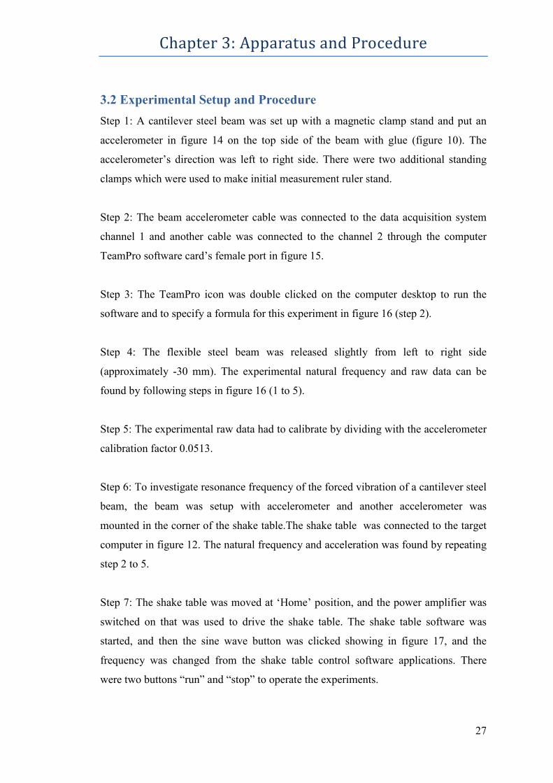
3.2 Experimental Setup and Procedure

Step 1: A cantilever steel beam was set up with a magnetic clamp stand and put an

accelerometer in figure 14 on the top side of the beam with glue (figure 10). The

accelerometer’s direction was left to right side. There were two additional standing

clamps which were used to make initial measurement ruler stand.

Step 2: The beam accelerometer cable was connected to the data acquisition system

channel 1 and another cable was connected to the channel 2 through the computer

TeamPro software card’s female port in figure 15.

Step 3: The TeamPro icon was double clicked on the computer desktop to run the

software and to specify a formula for this experiment in figure 16 (step 2).

Step 4: The flexible steel beam was released slightly from left to right side

(approximately -30 mm). The experimental natural frequency and raw data can be

found by following steps in figure 16 (1 to 5).

Step 5: The experimental raw data had to calibrate by dividing with the accelerometer

calibration factor 0.0513.

Step 6: To investigate resonance frequency of the forced vibration of a cantilever steel

beam, the beam was setup with accelerometer and another accelerometer was

mounted in the corner of the shake table.The shake table was connected to the target

computer in figure 12. The natural frequency and acceleration was found by repeating

step 2 to 5.

Step 7: The shake table was moved at ‘Home’ position, and the power amplifier was

switched on that was used to drive the shake table. The shake table software was

started, and then the sine wave button was clicked showing in figure 17, and the

frequency was changed from the shake table control software applications. There

were two buttons “run” and “stop” to operate the experiments.


28

Step 8: The experiment was started at 2 Hz frequency (without masses on top), and

“run” button was clicked. The shake table was started excited and then TeamPro

software was clicked to record experimental data. Step 4 was repeated to observe the

resonance frequency of a cantilever beam system. Different driving frequency was

increased until the beam had vibrated madly and located resonance frequency.

Step 9: Different masses were hanged ( 10 g, 20 g and 30 g ) on the top of a beam

right down side, next to the accelerometer in figure 13. The hanger (nuts and bolts)

weight was 5 g, and resonance frequency was found by repeating step 8 of a

cantilever steel beam.

Step 10: The experimental graphs were plotted and analysed by Matlab software.

CHAPT

HAPTER 4: EXPERIMEN

29

IMENT

Chapter 4: Experiment

30

4.1 Experiment 1

This experiment involves an analysis of free vibration of a cantilever steel beam

system and its mathematical modelling.

4.1.1 Experimental Data Analysis

The experimental data graph (figure 18) illustrates a simple harmonic motion graph,

and which oscillates with exponential amplitude. Assume the experimental data graph

is governed by well-known a sine function oscillations with exponential amplitude

equation. [7]

�� (t) = RPJQ�sin (�� + �) (21)

= logT ��E��5 (22)

Where:

R= is the amplitude [m/s2].

� = phase angle [radian].

�= natural frequency [rads/sec]. �� = acceleration [m/s2].

t = time [sec].

= log decrement of time displacement graph.


31

Figure 18 : Free vibration of a cantilever steel beam experiment-1 data. [ Also figure

18 Matlab code is available in appendix A.1.1].

4.1.2 Experimental Curve Fitting

The experimental data is plotted in Matlab software and it oscillates with exponential

amplitude. Two amplitudes, ��&(�&) = 6.929 m/s� and ��(��) = 6.282 m/s� where time, �&= 0.63 sec and �� = 0.99 sec and period, T = 0.4 sec are found in figure 19. Now the solutions are considered from the equation (21) and (22), i.e

Comments:

• Maximum acceleration about (+ 7.8 m/s2 and – 10.2 m/s

2).

• The oscillation amplitudes of (figure 18) decay with time because of

decaying exponential.


32

��&(�&) = RPJQ�&sin (��& + �) (23)

��(��)= RPJQ��sin (�� + �) (24)

= logT ��E��5 (25)

�= �\]^_`a$ (26)

Figure 19 : Free vibration of a cantilever steel beam experiment-1 data curve fitting.

The natural frequency can be calculated from equation (26), �= �\�.1 = 15.71 rads/sec

and log decrement from the graph (figure 19) = logT b.c�cb.�d� = 0.1 ; hence two simultaneous equations are placed; i.e


33

6.929 = RPJ(�.&∗�.bf)sin (15.71 ∗ 0.63 + �)

7.38= R sin ( 9.90 + �) (27)

6.282 = RPJ(�.&∗�.cc)sin (15.71 ∗ 0.99 + �)

6.94= R sin ( 15.55 + �) (28)

The equation (27) and (28) can be reduced the expression to simple sines and cosines

by using trigonometric identity

sin (A+B) = sin A cos B + cos A sin B (29)

Since the equation (27) and (28) by substituting trigonometry identity

7.38 = R [sin (9.90) cos� + cos (9.90)sin�]

7.38 = R [-0.46 cos� − 0.89 sin�] (30)

6.94 = R [sin (15.55) cos� + cos (15.55)sin�]

6.94 = R [0.16 cos� − 0.99 sin�] (31)

To find two unknown variables R and � , the equation (30) is divided by equation

(31) and the solution becomes

l.fdb.c1= J�.1b mnopJ�.dc oqrp�.&b mnopJ�.cc oqrp

-3.1924 cos� − 6.1766 sin� = 1.808 cos� − 7.3062 sin�

7.3062 sin� − 6.1766 sin� = 1.808 cos� + 3.1924 cos� 1.1296 sin� = 5.0004 cos� oqrpmnop= 4.43


34

tan� =4.43

� = tanJ& (4.43) = 1.35 rads

To find amplitude R, substitute � = 1.35 rads into equation (27); the solution can be

expressed as

R = l.fdoqr (c.c�t&.fu) = -7.62 m/s

2

So the theoretical acceleration solution for a cantilever steel beam will be

�� (t) = -7.62∗ PJ�.&∗�sin (15.71 ∗ � + 1.35 ) (32)

But if the equation (32) is integrated with respect to time, the theoretical velocity

solution for the beam will be found (�� (t)), and again integrate velocity with respect to time, the displacement will be placed ( �(�)) for vibration of a cantilever steel beam.

[The Matlab code to do integration with respect to t is in appendices A.1.10 ].

�� (t) = -7.62∗ PJ�.&∗�sin (15.71 ∗ � + 1.35)

�� (t) = 0.49∗ PJ�.&∗�cos (15.71 ∗ � + 1.35) + 0.0031∗ PJ�.&∗�sin (15.71 ∗ � + 1.35)

x (t) = -0.00039∗ PJ�.&∗�cos (15.71 ∗ � + 1.35)+ 0.03∗ PJ�.&∗�sin (15.71 ∗ � + 1.35)


35

4.1.3 Compare Experimental Results with Theory

Figure 20 : Compare vibration of a cantilever steel beam experiment-1 acceleration

results with theory. [Also graph Matlab code is available in appendix A.1.2].

Comments:

• Experimental maximum acceleration about (+ 7.8 m/s2 and – 10.2 m/s

2),

apparently theoretical maximum acceleration (+ 7.62 m/s2 and – 7.62 m/s

2)

in figure 20.

• Experimental oscillation amplitudes of (figure 20) more decay with time

than theoretical amplitudes.

• In actual practice the experimental system has always some damping (e.g.

the aero dynamical damping, the internal molecular friction and viscous

damping etc.) which makes decay of amplitude.


36

�� (t) = -7.62∗ PJ�.&∗�sin (15.71 ∗ � + 1.35) is a mathematical model for free

vibration of a cantilever steel beam. Velocity and displacement model equations can

be found by integrating acceleration with respect to time. The acceleration, velocity

and displacement graphs are established in figure 21 to compare experimental results.

Figure 21 : Compare acceleration, velocity and displacement of a cantilever steel

beam experiment-1 results. [ Also graph Matlab code is available in appendix A.1.3].

Comments:

• Maximum acceleration (+ 7.62 m/s2 and – 7.62 m/s

2), apparently maximum

velocity (+ 0.60 m/s and – 0.60 m/s) and maximum displacement (+ 0.03 m

and – 0.03 m) in figure 21.


37

Figure 22 : Free vibration of a cantilever steel beam experiment 1 displacement.

[Also graph Matlab code is available in appendix A.1.4].

Comments:

• Maximum displacement about (+ 0.03 m and – 0.03 m) in figure 22.

• The oscillation amplitudes of (figure 22) decay with time because of the

exponential function, x (t) = PJ�.&∗�. • The figure 22 does not undergo simple harmonic motion because the

acceleration is not proportional to the displacement.


38

4.2 Experiment 2

This experiment involves an analysis of a forced vibration of a cantilever stainless

steel beam and its resonance frequency. In fact, different masses (15 g, 25 g and 35 g)

were put on top of a cantilever steel beam. The beam was driven by force frequency

through the base excitation shake table.

4.2.1 Theoretical Data Analysis

From the theory of a vibration structure system, the transverse deflection of a

cantilever stainless steel beam is equivalent to a single degree spring mass system.

Hence the equation can be written: [1]

� = f��v� (33)

Where:

� = thickness of a steel beam[N/m].

w = the Young’s modulus [N/m2] .

x = the second moment of area [ m4].

y = length of a steel beam [m].

However, the second moment of area of the beam can be written as equation (34),

where b and d are the breadth and width of the experimental beam.

x = z$�&� (34)


39

The natural frequency of the stainless steel beam in transverse direction is given by

� = � A{|}|~� (35)

Where ��a�� is the total mass of the steel beam, so the equation can be written as

(36)

��a�� = @z^�B + @�""�^_aB^�^_ + @ ^`�� (36)

mass=15g, 25g, 35g

l =285 mm d=0.51 mm

b=31.59 mm

accelerometer

Figure 23 : Experiment-2 theoretical natural frequency analysis.


40

Table 1 : Theoretical natural frequency in different masses of a steel beam

Mass @z^�B

kg

Mass @�""�

kg

Mass @ ^`��

kg

Total

Mass ��a��

kg

Beam

Length

L

m

Moment

Inertia

x = ��f12

m4

Young’s

Modulus

Stainless

Steel

E

N/m2

Beam

Stiffness

� = 3wx�f

N/m

Natural

Frequency �= � ��a��

rads/sec

0.03 0.0046 0

0.0345 0.285 3.49× 10J&f 1.8× 10&& 8.146 15.37

0.03 0.0046 0.015

0.0496 0.285 3.49× 10J&f 1.8× 10&& 8.146 12.82

0.03 0.0046 0.020

0.0546 0.285 3.49× 10J&f 1.8× 10&& 8.146 12.22

0.03 0.0046 0.035

0.0696 0.285 3.49× 10J&f 1.8× 10&& 8.146 10.82

Comments:

The natural frequency� is decreasing by increasing the mass on the top of a

cantilever beam (Table 1). In fact the theoretical �=15.37 rads/sec is almost same

as the free vibration of a cantilever steel beam natural frequency�=15.71 rads/sec in figure 19.


41

4.2.2 Experimental Data Analysis

Figure 24 : Compare experimental natural frequency with changes mass on the top of

a cantilever beam. [ Also graph Matlab code is available in appendix A.1.5].

The experimental graph illustrates (figure 25, 26, 27 and 28) a simple harmonic

motion, and which has a solution of the form �� (t) = A sin (�� + �), where A is a

amplitude, � natural frequency of oscillation of the function articulated as radians per unit time, and � is a phase angle unit radian. The related frequency is cycles per

unit time is represented by f ; and consider � = 2�� where frequency unit is Hz. [7]

Comments:

• The natural frequency varies to change the mass on top of a cantilever

beam.

• The oscillation amplitudes of (figure 24) decay with time because of

decaying exponential.


42

4.2.2.1 Forced Vibration Resonance without Mass on Top

Figure 25 : Forced vibration experiment-2 resonance frequency (no mass) on the top

of a steel beam. [Also graph Matlab code is available in appendix A.1.6].

Comments:

• (In figure 25a) Maximum acceleration about (+ 17.58 m/s2 and – 17.58

m/s2), and driving frequency, � = 2.6 Hz which is less than natural

frequency, � = 2.897 Hz. • (In figure 25b) Maximum acceleration about (+ 37.22 m/s

2 and – 37.22

m/s2), and driving frequency, � = 2.7 Hz which is less than natural

frequency, � = 2.897 Hz. There is some resonance frequency in the

system.

• (In figure 25c) Maximum acceleration about (+ 50.66 m/s2 and – 50.66

m/s2), and driving frequency, � = 2.8 Hz which is almost same to natural

frequency, � = 2.897 Hz. • (In figure 25d) Maximum acceleration about (+ 62.35 m/s

2 and – 62.35

m/s2), and driving frequency, � = 2.9 Hz which is almost same to natural

frequency, � = 2.897 Hz.


43

4.2.2.2 Forced Vibration Resonance 15 g Mass on Top

Figure 26 : Forced vibration experiment-2 resonance frequency 15 g mass on the top


Comments:

• (In figure 26a) Maximum acceleration about (+ 4.74 m/s2 and – 4.74 m/s

2),

and driving frequency, � = 1.5 Hz which is less than natural frequency, � = 1.842 Hz.

• (In figure 26b) Maximum acceleration about (+ 14.01 m/s2 and – 14.01

m/s2) and driving frequency, � = 1.7 Hz which is less than natural


system.


m/s2) and driving frequency, � = 1.8 Hz which is equal to natural

frequency, � = 1.842 Hz. • (In figure 26d) Maximum acceleration about (+ 19.26 m/s

2 and – 19.26

m/s2) and driving frequency, � = 1.9 Hz which is almost equal to natural



44




Comments:


2),


• (In figure 27b) Maximum acceleration about (+ 6.02 m/s2 and – 6.02 m/s

2)





system.

• (In figure 27d) Maximum acceleration about (+ 19.94 m/s2 and – 19.94

m/s2) and driving frequency, � = 1.5 Hz which is almost equal to natural



45




Comments:


2),

and driving frequency, � = 0.90 Hz which is less than natural frequency,

� = 1.208 Hz. • (In figure 28b) Maximum acceleration about (+ 2.48 m/s

2 and – 2.48 m/s

2)


• (In figure 28c) Maximum acceleration about (+ 6.70 m/s2 and – 6.70 m/s

2)


• (In figure 28d) Maximum acceleration about (+ 17.28 m/s2 and – 17.28



system.

CHAP

HAPTER 5: DISCUSSIO

46

SSION

Chapter 5: Discussion

47

5.1 Discussion

The project argues that theoretically calculated natural frequency of the vibration of a

cantilever steel beam is different from experimental results in experiment 1 and

experiment 2. However, better results can be found for natural frequency to correct

the mass of an accelerometer. The cantilever steel beam was fixed at one side; in

actual engineering practice flexibility in support may affect the natural frequency.

The theoretical maximum acceleration was approximately ±7.62 m/s2.Consequently,

it was also found that the experimental maximum positive acceleration was about

+7.8 m/s2 and negative acceleration was about -10.2 m/s

2. In fact, the experimental

amplitude had been changed due to damping in the system (e.g. the aero dynamical

damping, the internal molecular friction and viscous damping etc.) in figure 20. In

practice, the oscillation amplitudes of the mathematical model equation decay with

time because of the exponential function, �� (t) = PJ�.&∗�. A displacement represented

in figure 22 does not endure simple harmonic motion because the acceleration is not

proportional to the displacement.

The maximum initial displacement of the vibration of a cantilever steel beam was

found around ± 0.03 m, and which was same as we had an experimental initial

disturbance in figure 10.

The resonance frequency of the forced vibration of a cantilever steel beam was

slightly different to the theory due to wrong estimated natural frequency in

experiment 2. The graph is shown in figure 26; increasing the mass on top of the

beam is decreasing the natural frequency of the vibration of a cantilever steel beam.

In experiment 2, it was observed that experimentally resonance frequency was only

occurred when the natural frequency was equal to the driving frequency ( � = �),

and then the maximum acceleration amplitude increased madly in figure (27-30).

CHAPTER 6:

AND

APTER 6: RECOMMENDATIO

AND CONCLUSION

48

ENDATIONS

Chapter 6: Recommendations and Conclusion

49

6.1 Conclusion

This project investigates the vibration of a cantilever steel beam by comparing the

theory with the experimental results. In particular, this project examines, both

theoretically and experimentally, that the free vibration of a cantilever beam involves

continuous systems and the forced vibration is subjected to transverse harmonic

excitation. Moreover, this project observes the effects of resonance frequency in

forced vibration on mass top or without mass of a cantilever steel beam, and the drive

force frequency by base excitation shake table. The project is associated with two

theories (a) ‘Lateral Vibration of Beam’ (b) ‘Forced Vibration Spring-Mass System’.

In practice, this project observes that the lateral vibration of beam is considered as

continuous systems which have their mass and stiffness spread out continuously

across the whole system and vibrates at one or more of its natural frequency.

The vibration of a cantilever steel beam theory has two solutions: one is Ordinary

Differential Equation (ODE), and another one is Partial Differential Equation (PDE).

In fact, ODE has only one independent variable but in case of PDE, it has two or more

independent variables. The vibration of a cantilever steel beam theory involves two

variables which are time (t) and beam arc length (x) so that the solution of the beam

will be PDE. The time displacement response is solved by simple harmonic motion

equation and arc length can be solved by trigonometric hyperbolic functions.

However, the vibration of a cantilever steel beam solutions can be solved by two

initial conditions and four boundary conditions. In this project, the curve fitting

method was used to make a mathematical modeling equation of the free vibration of a

cantilever steel beam.

This project only examines the vibration of a cantilever beam’s time displacement not

mode shape ( W ). In fact, the vibration of a cantilever steel beam has an infinite

number of normal modes with one natural frequency associated with each normal

mode.


50

Experimentally it was also observed that the simple harmonic motion with

exponential amplitude equation is valid for free vibration of a cantilever steel beam

system. In fact, a mathematical model [�� (t) = -7.62∗ PJ�.&∗�sin (15.71 ∗ � + 1.35 )] has been established from the experimental results of the free vibration of a cantilever

steel beam. Subsequently, this project shows that the theoretically calculated natural

frequency is slightly different from the experimental natural frequency. However,

better results can be found for natural frequency to correct the mass of accelerometer.

The forced vibration of a cantilever steel beam has single degrees of freedom. In

engineering, when an external force is driven in any system, the resulting vibration is

known as forced vibration. If the frequency of external forces vibration matches with

natural frequencies of the system then resonance frequency occurs. Experimentally

this project shows that if the natural frequency (�) of the beam matches with

external driving frequency ( �), the maximum amplitude is conducted.

This project theoretically investigates that a cantilever steel beam is fixed at end can

be idealized as spring mass system in figure 23. The beam top mass can be considered

as point mass and the beam structure can be approximated as a spring to get single

degrees of freedom. In fact, the spring thickness ( k ) is merely the ratio of force

deflection, and it can be expressed from the geometric and materials properties of the

beam columns. The mass of a cantilever will be same as that of the floor if assume the

mass of the beam column to be negligible. [1]


51

6.2 Recommendations for Future Work

In this project, ‘vibration of a cantilever beam’ was investigated subject to lateral

vibration of a cantilever steel beam which is fixed at end and the forced vibration

resonance frequency by driving external force into a system. The free vibration of a

cantilever steel beam mathematical modeling equation can be used to implement

engineering applications failure.

This project was investigated only the vibration of a cantilever beam which is fixed at

end. However, in future the investigation will be conducted on different types of beam

fixed-fixed, fixed-pinned, pinned-free and so on. It will be interesting to see the

vibration of a cantilever beam mode shapes and degrees of freedom under different

end conditions of beam.

The resonance frequency is one of the main causes of wind turbines tower failure. In

future, it will be great opportunity to work on wind turbines and other application

which is related to resonance frequency of dynamics systems.

CHAPT

HAPTER 7: REFERENCE

52

ENCES

Chapter 7: References

53

1. Rao, S.S. (2003) Mechanical vibration: free vibration of single degree of

freedom system, continuous systems. 4th edition. New Jersey: Pearson

Education Ltd.

2. Timoshenko, P.S. & Gere, J.M. (1961) Theory of elastic stability. 2nd Edition.

USA: The Maple Press Company, York, PA.

3. Meriam, J.L. and Kraige, L.G. (2007) Engineering mechanics dynamics:

vibration and time response. 6th edition. USA: John Wiley & Sons.

4. Struik, D.J. (1948) A concise history of mathematics. 2nd edition. New York:

Dover Publications Inc.

5. Saint-Petersburg State Polytechnic University (2012), Structural mechanics

and theory of elasticity department [Online] Available from:

(http://smitu.cef.spbstu.ru/timoshenko_en.htm) [Accessed on 10th Feb, 2012]

6. Meirovitch, L. (1967) Analytical methods in vibration, London: Ccollier-

Macmillan.

7. Palm III, W. J. (2007) Mechanical vibration: descriptions of vibration

motions. USA: John Wiley & Sons.

8. Hitomi, K. (1996) Manufacturing systems engineering. 2nd edition. London:

Taylor & Francis.


54

9. Turbo Squid (2012), 3d model wind turbine[Online] Available

from:(http://www.turbosquid.com/3d-models/3d-model-windturbine/581029

[Accessed on 1st April, 2012]

10. Goss, D.G. (2011) Dynamics and system modeling 3. Lecture Notes. London:

London South Bank University.

11. Cutcaster Photo (2012), Galileo-Galilei picture [Online] Available from:

( http://cutcaster.com/photo/100511943-Galileo-Galilei/) [Accessed on 28th

April, 2012]

12. Shetland Times (2012), Wind turbines tower collapse picture [Online]

Available from:(http://www.shetlandtimes.co.uk/2012/01/19/deal-likely-

within-weeks-to-help-owners-of-faulty-wind-turbines) [Accessed on 29th

April, 2012]

13. Pugwash windfarm (2012) Wind turbines tower failure picture[Online]

Available from:( http://pugwashwindfarm.blogspot.co.uk/2007/08/man-killed-

after-wind-tower-collapses.html) [Accessed on 29th April, 2012]

14. Thomson, W.T. & Dalhleh, M.D. (1998) Theory of vibration with

applications: free vibration, harmonically excited vibration, vibration of

continuous systems. 5th edition. USA: Prentice Hall, Inc.


55

15. More, H. (2009) Matlab for engineers: plotting, symbolic mathematics. 2nd

edition. New Jersey: Pearson, Prentice Hall.

16. Hopekins, R.B. (1970) Design analysis of shafts and beams: cantilever

beams.USA: McGraw-Hill, Inc

17. Wahab, M.A. (2008) Dynamics and vibration. UK: Wiley & Sons Ltd.

18. Dixit, U.S. (2009) Finite element methods for engineers. Delhi: Cengage

Learning India Pvt, Ltd.

List

List of Appendices

56

Appendix: A

57

Appendix: A

58

% MATLAB CODE FOR EXPERIMENT-1 GRAPH ( experimental data) A= xlsread( 'test1.xls' ) B= xlsread( 'test2.xls' ) % Create xlabel xlabel( 'Time (sec)' ); % Create ylabel ylabel( 'Acceleration (ms^-2)' ); % Create title title( 'Graph: Compare vibration of a cantilever steel be am experiment-1 acceleration results with theory' ); hold on; plot(A,B, 'r' )

A.1 Matlab Code

A.1.1 Figure 18: Free vibration of a cantilever steel beam experiment-1

data matlab code.

Appendix: A

59

% MATLAB CODE FOR EXPERIMENT-1 GRAPH (compare exper imental data with theory) t=0:0.002:8.191; %time % Initial values for experiment. R=-7.62; % m/s^2 lamda=0.1; % fy=1.35; % rads wn=15.71; % rad/sec k=(R.*exp(-lamda.*t).*sin(wn.*t+fy)) plot(t,k) box( 'on' ); hold( 'all' ); % Create xlabel xlabel( 'Time (sec)' ); % Create ylabel ylabel( 'Distance (m)' ); % Create title title( 'graph: distance vs time' ); hold on; A= xlsread( 'test1.xls' ) B= xlsread( 'test2.xls' ) % Create xlabel xlabel( 'Time (sec)' ); % Create ylabel ylabel( 'Acceleration (ms^-2)' ); % Create title title( 'Graph: Compare vibration of a cantilever steel be am experiment-1 acceleration results with theory' ); hold on; plot(A,B, 'r' )

A.1.2 Figure 20: Compare vibration of a cantilever steel beam experiment-

1 acceleration results with theory matlab code.

Appendix: A

60

%MATLAB CODE TO COMPARE EXPERIMENT 1 ACCELERATION, VELOCITY AND %DISPLACEMENT t=0:0.002:8.191; %time % Initial values for experiment. % Create xlabel xlabel( 'Time (sec)' ); % Create ylabel ylabel( 'Amplitude' ); % Create title title( 'Graph: Compare acceleration, velocity and displace ment of a cantilever steel beam experment-1 results' ); k=(-7.62.*exp(-0.1.*t).*sin(15.71.*t+1.35)) % ACCELERATION plot(t,k, 'r' ) hold on; m=(0.49.*exp(-0.1.*t).*cos(15.71.*t+1.35)+0.0031.*e xp(-0.1.*t).*sin(15.71.*t+1.35)) % VELOCITY plot(t,m, 'b' ) hold on; p=(-0.00039.*exp(-0.1.*t).*cos(15.71.*t+1.35)+0.03. *exp(-0.1.*t).*sin(15.71.*t+1.35)) % DISPLACEMENT plot(t,p, 'g' ) box( 'on' );

A.1.3 Figure 21: Compare acceleration, velocity and displacement of a

cantilever steel beam experiment-1 results.

Appendix: A

61

% MATLOB CODE FOR EXPERIMENT 1 GRAPH(experiment 1 d isplacement) t=0:0.002:8.191; %time % Initial values for experiment. % Create xlabel xlabel( 'Time (sec)' ); % Create ylabel ylabel( 'Displacement (m)' ); % Create title title( 'Graph: Free vibration of a cantilever steel beam e xperment-1 displacement' ); p=(-0.00039.*exp(-0.1.*t).*cos(15.71.*t+1.35)+0.03. *exp(-0.1.*t).*sin(15.71.*t+1.35)) plot(t,p, 'b' ) box( 'on' );

A.1.4 Figure 22: Free vibration of a cantilever steel beam experiment 1

displacement.

Appendix: A

62

% MATLAB CODE FOR Experiment 2 (Compare natural fr equency) A= xlsread( 'resonance_time.xls' ); B= xlsread( 'n.xls' ); % Create xlabel xlabel( 'Time (sec)' ); % Create ylabel ylabel( 'Amplitude' ); % Create title title( 'Graph : Compare experimental natural frequency wit h changes mass on the top of a cantilever steel beam' ); plot(A,B, 'r' ) hold on; C= xlsread( 'resonance_time.xls' ); D= xlsread( 'n15gram.xls' ); plot(C,D, 'b' ) hold on; E= xlsread( 'resonance_time.xls' ); F= xlsread( 'n25gram.xls' ); plot(E,F, 'g' ) hold on; G= xlsread( 'resonance_time.xls' ); H= xlsread( 'n35gram.xls' ); plot(G,H, 'm' ) hold on;

A.1.5 Figure 24: Compare experimental natural frequency with changes

mass on the top of a cantilever beam.

Appendix: A

63

% MATLAB CODE FOR EXPERIMENT-2 GRAPH (0g mass on th e top of a beam) A= xlsread( 'resonance_time.xls' ) B= xlsread( 'resonance_0gram_2p6.xls' ) % Create xlabel xlabel( 'Time (sec)' ); % Create ylabel ylabel( 'Acceleration (ms^-2)' ); % Create title title( 'Figure- 15a : Experiment 2 driving frequency (w = 2.6 Hz )' ); subplot(2,2,1) plot(A,B, 'r' ) C= xlsread( 'resonance_time.xls' ) D= xlsread( 'resonance_0gram_2p7.xls' ) % Create xlabel xlabel( 'Time (sec)' ); % Create ylabel ylabel( 'Acceleration (ms^-2)' ); % Create title title( 'Figure- 15b : Experiment 2 driving frequency (w = 2.7 Hz )' ); subplot(2,2,2) plot(C,D, 'b' ) E= xlsread( 'resonance_time.xls' ) F= xlsread( 'resonance_0gram_2p8.xls' ) % Create xlabel xlabel( 'Time (sec)' ); % Create ylabel ylabel( 'Acceleration (ms^-2)' ); % Create title title( 'Figure- 15c : Experiment 2 driving frequency (w = 2.8 Hz )' ); subplot(2,2,3) plot(E,F, 'g' ) G= xlsread( 'resonance_time.xls' ) H= xlsread( 'resonance_0gram_2p9.xls' ) % Create xlabel xlabel( 'Time (sec)' ); % Create ylabel ylabel( 'Acceleration (ms^-2)' ); % Create title title( 'Figure- 15d : Experiment 2 driving frequency (w = 2.9 Hz )' ); subplot(2,2,4) plot(G,H, 'm' )

A.1.6 Figure 25: Forced vibration experiment-2 resonance frequency (no

mass) on the top of a steel beam.

Appendix: A

64

% MATLAB CODE FOR EXPERIMENT-2 GRAPH(15g mass on th e top of a beam) A= xlsread( 'resonance_time.xls' ) B= xlsread( 'resonance_15gram_1p5.xls' ) % Create xlabel xlabel( 'Time (sec)' ); % Create ylabel ylabel( 'Acceleration (ms^-2)' ); % Create title title( 'Figure- 16a : Experiment 2 driving frequency (w = 1.5 Hz )' ); subplot(2,2,1) plot(A,B, 'r' ) C= xlsread( 'resonance_time.xls' ) D= xlsread( 'resonance_15gram_1p7.xls' ) % Create xlabel xlabel( 'Time (sec)' ); % Create ylabel ylabel( 'Acceleration (ms^-2)' ); % Create title title( 'Figure- 16b : Experiment 2 driving frequency (w = 1.7 Hz )' ); subplot(2,2,2) plot(C,D, 'b' ) E= xlsread( 'resonance_time.xls' ) F= xlsread( 'resonance_15gram_1p8.xls' ) % Create xlabel xlabel( 'Time (sec)' ); % Create ylabel ylabel( 'Acceleration (ms^-2)' ); % Create title title( 'Figure- 16c : Experiment 2 driving frequency (w = 1.8 Hz )' ); subplot(2,2,3) plot(E,F, 'g' ) G= xlsread( 'resonance_time.xls' ) H= xlsread( 'resonance_15gram_1p9.xls' ) % Create xlabel xlabel( 'Time (sec)' ); % Create ylabel ylabel( 'Acceleration (ms^-2)' ); % Create title title( 'Figure- 16d : Experiment 2 driving frequency (w = 1.8 Hz )' ); subplot(2,2,4) plot(G,H, 'm' )

A.1.7 Figure 26: Forced vibration experiment-2 resonance frequency 15 g

mass on the top of a steel beam.

Appendix: A

65

% MATLAB CODE FOR EXPERIMENT-2 GRAPH(25g mass on th e top of a beam) A= xlsread( 'resonance_time.xls' ) B= xlsread( 'resonance_25gram_1p2.xls' ) % Create xlabel xlabel( 'Time (sec)' ); % Create ylabel ylabel( 'Acceleration (ms^-2)' ); % Create title title( 'Figure- 17a : Experiment 2 driving frequency (w = 1.2 Hz )' ); subplot(2,2,1) plot(A,B, 'r' ) C= xlsread( 'resonance_time.xls' ) D= xlsread( 'resonance_25gram_1p3.xls' ) % Create xlabel xlabel( 'Time (sec)' ); % Create ylabel ylabel( 'Acceleration (ms^-2)' ); % Create title title( 'Figure- 17b : Experiment 2 driving frequency (w = 1.3 Hz )' ); subplot(2,2,2) plot(C,D, 'b' ) E= xlsread( 'resonance_time.xls' ) F= xlsread( 'resonance_25gram_1p4.xls' ) % Create xlabel xlabel( 'Time (sec)' ); % Create ylabel ylabel( 'Acceleration (ms^-2)' ); % Create title title( 'Figure- 17c : Experiment 2 driving frequency (w = 1.4 Hz )' ); subplot(2,2,3) plot(E,F, 'g' ) G= xlsread( 'resonance_time.xls' ) H= xlsread( 'resonance_25gram_1p5.xls' ) % Create xlabel xlabel( 'Time (sec)' ); % Create ylabel ylabel( 'Acceleration (ms^-2)' ); % Create title title( 'Figure- 17d : Experiment 2 driving frequency (w = 1.5 Hz )' ); subplot(2,2,4) plot(G,H, 'm' )



Appendix: A

66

% MATLAB CODE FOR EXPERIMENT-2 GRAPH(35g mass on th e top of a beam) A= xlsread( 'resonance_time.xls' ) B= xlsread( 'resonance_35gram_0p90.xls' ) % Create xlabel xlabel( 'Time (sec)' ); % Create ylabel ylabel( 'Acceleration (ms^-2)' ); % Create title title( 'Figure- 18a : Experiment 2 driving frequency (w = 0.90 Hz )' ); subplot(2,2,1) plot(A,B, 'r' ) C= xlsread( 'resonance_time.xls' ) D= xlsread( 'resonance_35gram_1p0.xls' ) % Create xlabel xlabel( 'Time (sec)' ); % Create ylabel ylabel( 'Acceleration (ms^-2)' ); % Create title title( 'Figure- 18b : Experiment 2 driving frequency (w = 1.0 Hz )' ); subplot(2,2,2) plot(C,D, 'b' ) E= xlsread( 'resonance_time.xls' ) F= xlsread( 'resonance_35gram_1p1.xls' ) % Create xlabel xlabel( 'Time (sec)' ); % Create ylabel ylabel( 'Acceleration (ms^-2)' ); % Create title title( 'Figure- 18c : Experiment 2 driving frequency (w = 1.1 Hz )' ); subplot(2,2,3) plot(E,F, 'g' ) G= xlsread( 'resonance_time.xls' ) H= xlsread( 'resonance_35gram_1p2.xls' ) % Create xlabel xlabel( 'Time (sec)' ); % Create ylabel ylabel( 'Acceleration (ms^-2)' ); % Create title title( 'Figure- 18c : Experiment 2 driving frequency (w = 1.2 Hz )' ); subplot(2,2,4) plot(G,H, 'm' )



Appendix: A

67

%MATLAB CODE FOR EXPERIMENT 1 TO DO INTEGRATION WITH RESPECT TIME

% integration to find velocity velocity=sym( '(-7.62*exp(-0.1*t)*sin(15.71*t+1.35))' ) int(velocity, 't' ) % integration to find displacement disp=sym( '(0.49*exp(-0.1*t)*cos(15.71*t+1.35)+0.0031*exp(-0.1*t)*sin(15.71*t+1.35))' ) int(disp, 't' )

A.1.10 Integration with respect to time.

Project Planning

68

Project Planning

69

B.1 Project Planning Schedule

The project has started from 7th of Oct, 2011. The approximate action plan of

activities for my project is shown below on the Gantt chart.

October 2011 to May 2012

Months Oct

2011

Nov

2011 Dec

2011 Jan

2012 Feb

2012 Mar

2012 Apr

2012 May

2012

Weeks 1 2 3 4 1 2 3 4 1 2 3 4 1 2 3 4 1 2 3 4 1 2 3 4 1 2 3 4 1 2 3 4

Task

Task 1

Task 2

Task 3

Task 4

Task 5

Task 6

Task 7

Task 8

Task 9

Task 10

Task 11

Task 1 = Project arrangement form.

Task 2 = Project theory study.

Task 3 = Project brief.

Task 4 = Project specification, work schedule and costing.

Task 5 = Experimental work.

Task 6 = Experimental results analysis.

Task 7 = Project review and target setting.

Task 8 = Interim report.

Task 9 = Final project e-report through TURNITION for

plagiarism checking.

Task 10 = Project report writing.

Task 11 = Project Background study.

faculty of e lty of engineering, science and the nd the built …€¦ · · 2015-10-08lty of...

Documents