faculty of sciences bayesian methods in arti...
TRANSCRIPT

Faculty of Sciences
Bayesian Methods in Artificial Neural Networks
Ben Meuleman
Master dissertation submitted toobtain the degree of
Master of Statistical Data Analysis
Promoter: Prof. Dr. Rene BoelCo-promoter: Prof. Dr. Stefan Van Aelst
Tutor: Dr. Wim De Mulder
Department of Applied Mathematics
Academic year 2011–2012

The author and the promoter give permission to consult this master dissertation and tocopy it or parts of it for personal use. Each other use falls under the restrictions of thecopyright, in particular concerning the obligation to mention explicitly the source when
using results of this master dissertation.

Foreword
This thesis would not be complete without an acknowledgment to all those that directly orindirectly contributed to this work. First of all, I would like to thank Rene Boel and WimDe Mulder for supervising this project over the course of three long years. I have tested theirendurance on this project for much longer than should have been necessary, and thereforethank them for their patience. Wim De Mulder in particular I thank for mathematicaltutoring. Second, I thank Stefan Van Aelst for offering advice and practical suggestions, andfor agreeing to co-supervise this thesis at the last minute. Third, I thank Ian Nabney for hishelpful correspondence on modeling issues, and whose NETLAB software was inspirationalfor my own R script.
I also thank my MASTAT peers, Johan Steen, Joke Durnez and Sanne Roels, whomI have known since studying psychology and whose presence and mutual support made theMASTAT program a very enjoyable experience.
On a more general note, I would like to thank the teachers of the MASTAT program,Stijn Vansteelandt, Els Goetghebeur, Olivier Thas, and Tom Loeys, for their clear and enthu-siastic way of teaching statistics, and for their accessibility in offering advice and helping outwith problems. Finally, I would like to thank Yves Rosseel, whose courses in data analysis atthe Faculty of Psychology inspired me to take up statistics in the first place.

Contents
1 Introduction 1
2 Artificial neural networks 22.1 Basics . . . . . . . . . . . . . . . . . . . . . . . . . . . . . . . . . . . . . . . . 22.2 Network structure . . . . . . . . . . . . . . . . . . . . . . . . . . . . . . . . . 32.3 Optimization . . . . . . . . . . . . . . . . . . . . . . . . . . . . . . . . . . . . 6
2.3.1 Principles . . . . . . . . . . . . . . . . . . . . . . . . . . . . . . . . . . 62.3.2 Gradient descent . . . . . . . . . . . . . . . . . . . . . . . . . . . . . . 62.3.3 Newton’s method . . . . . . . . . . . . . . . . . . . . . . . . . . . . . . 72.3.4 The BFGS algorithm . . . . . . . . . . . . . . . . . . . . . . . . . . . . 72.3.5 Optimization in practice . . . . . . . . . . . . . . . . . . . . . . . . . . 8
2.4 Example . . . . . . . . . . . . . . . . . . . . . . . . . . . . . . . . . . . . . . . 9
3 Bayesian neural networks 123.1 Motivation . . . . . . . . . . . . . . . . . . . . . . . . . . . . . . . . . . . . . 123.2 Principles . . . . . . . . . . . . . . . . . . . . . . . . . . . . . . . . . . . . . . 12
3.2.1 Likelihood . . . . . . . . . . . . . . . . . . . . . . . . . . . . . . . . . . 133.2.2 Prior . . . . . . . . . . . . . . . . . . . . . . . . . . . . . . . . . . . . . 133.2.3 Posterior distribution . . . . . . . . . . . . . . . . . . . . . . . . . . . 14
3.3 Gaussian approximation . . . . . . . . . . . . . . . . . . . . . . . . . . . . . . 163.3.1 Posterior distribution of the weights . . . . . . . . . . . . . . . . . . . 163.3.2 Estimation of hyperparameters . . . . . . . . . . . . . . . . . . . . . . 173.3.3 Comparing the evidence for different networks . . . . . . . . . . . . . 183.3.4 Automatic Relevance Determination . . . . . . . . . . . . . . . . . . . 19
3.4 Computational addenda to the Bayesian method . . . . . . . . . . . . . . . . 203.4.1 Initial network settings . . . . . . . . . . . . . . . . . . . . . . . . . . 203.4.2 Reestimation of hyperparameters . . . . . . . . . . . . . . . . . . . . . 203.4.3 Model evidence . . . . . . . . . . . . . . . . . . . . . . . . . . . . . . . 21
3.5 Numerical implementation of the Bayesian method . . . . . . . . . . . . . . . 223.6 Example . . . . . . . . . . . . . . . . . . . . . . . . . . . . . . . . . . . . . . . 22
3.6.1 Evidence ranking . . . . . . . . . . . . . . . . . . . . . . . . . . . . . . 233.6.2 Model inspection . . . . . . . . . . . . . . . . . . . . . . . . . . . . . . 24
4 Present study 254.1 Objectives . . . . . . . . . . . . . . . . . . . . . . . . . . . . . . . . . . . . . . 254.2 Problems of model selection . . . . . . . . . . . . . . . . . . . . . . . . . . . . 26
4.2.1 Number of reestimation cycles . . . . . . . . . . . . . . . . . . . . . . 264.2.2 Evidence as a model selection criterion . . . . . . . . . . . . . . . . . . 274.2.3 ARD pruning . . . . . . . . . . . . . . . . . . . . . . . . . . . . . . . . 27
5 Method 285.1 Calibration phase . . . . . . . . . . . . . . . . . . . . . . . . . . . . . . . . . . 28
5.1.1 Convergence of network evidence . . . . . . . . . . . . . . . . . . . . . 285.1.2 Evidence as a model selection criterion . . . . . . . . . . . . . . . . . . 295.1.3 Automatic Relevance Determination . . . . . . . . . . . . . . . . . . . 29

5.2 Application phase . . . . . . . . . . . . . . . . . . . . . . . . . . . . . . . . . 305.2.1 Forest Fires data . . . . . . . . . . . . . . . . . . . . . . . . . . . . . . 315.2.2 Concrete Compressive Strength data . . . . . . . . . . . . . . . . . . . 325.2.3 California Housing data . . . . . . . . . . . . . . . . . . . . . . . . . . 33
5.3 Software . . . . . . . . . . . . . . . . . . . . . . . . . . . . . . . . . . . . . . . 34
6 Results 356.1 Calibration phase . . . . . . . . . . . . . . . . . . . . . . . . . . . . . . . . . . 35
6.1.1 Convergence of network evidence . . . . . . . . . . . . . . . . . . . . . 356.1.2 Evidence as a model selection criterion . . . . . . . . . . . . . . . . . . 366.1.3 Automatic Relevance Determination . . . . . . . . . . . . . . . . . . . 426.1.4 Conclusions of calibration phase . . . . . . . . . . . . . . . . . . . . . 47
6.2 Application phase . . . . . . . . . . . . . . . . . . . . . . . . . . . . . . . . . 486.2.1 Forest Fires data . . . . . . . . . . . . . . . . . . . . . . . . . . . . . . 486.2.2 Concrete Compressive Strength data . . . . . . . . . . . . . . . . . . . 506.2.3 California Housing data . . . . . . . . . . . . . . . . . . . . . . . . . . 52
7 Discussion 557.1 Model selection strategy . . . . . . . . . . . . . . . . . . . . . . . . . . . . . . 567.2 Applying Bayesian neural networks in practice . . . . . . . . . . . . . . . . . 577.3 Conclusion . . . . . . . . . . . . . . . . . . . . . . . . . . . . . . . . . . . . . 58
8 References 58
Appendix - BFNN documentation 61

1 Introduction
Bayesian methods extend traditional feedforward neural networks by formalizing certain as-
pects of model building such as the choice of architecture, the estimation of control parameters
and selection of input variables. Increasingly, such models have been successfully applied to
complex problems of machine learning and pattern recognition [1, 2]. One of the most widely
used approaches to Bayesian neural networks is the evidence framework developed by MacKay
[3]. The evidence framework utilizes a Gaussian approximation to calculate the posterior dis-
tribution of the network weights and to find plausible values for hyperparameters. In addition,
the method allows to rank different networks by their plausibility according to the so-called
evidence information criterion, and to automatically determine the predictive relevancy of
input variables without the need for cross-validation. Applying the evidence framework in
practice requires several choices to be made, including the number of reestimation cycles
for optimizing the network (hyper)parameters, and which model to use for deriving variable
relevancies. At present, these choices are addressed in an ad-hoc manner by researchers.
For this thesis, I reexamined the usefulness of the evidence framework as an approach
to model selection and interpretation. In a first phase, I used an artificial dataset to derive a
suitable modeling strategy, investigating (a) the utility of model evidence to choose an optimal
network architecture, (b) how the number of reestimation cycles influences the evidence of
a model, and (c) how an appropriate model for relevance determination should be chosen.
To accomplish this, I systematically varied the number of reestimation cycles for parameter
optimization, the size of the network, the available training data, and the number of irrelevant
predictors in the dataset. In the second phase, I applied the derived strategy to three real
univariate regression problems: the Forest Fires data, the Concrete Compressive Strength
data, and the California Housing data. I compared performance of the Bayesian neural
network to the standard neural network in terms of predictive accuracy (test error) as well as
the total computation time required to apply each method. Computations were carried out
using a custom program written in the R statistical software.
This text is organized as follows. In the second chapter, the basics of the classical
feedforward neural network are described and illustrated by example. In the third chapter,
the Bayesian approach to neural networks is explained in detail and illustrated by example.
The remainder of the thesis is dedicated to the application of Bayesian neural networks in the
manner described above. The appendix, finally, contains details about the R software that
was written for this thesis.
1

2 Artificial neural networks
2.1 Basics
Artificial neural networks are a class of statistical models that were developed independently
in several fields throughout the 20th Century, including statistics, artificial intelligence, and
neuroscience. In their earliest form, such models were used to simulate neuronal processes
inside the human brain [4], hence their name. A neural network typically consists of compu-
tational units connected by layers of weights, processing information in a parallel distributed
fashion. Many types of such networks have been proposed, each with varying degrees of
architectural complexity. Throughout this thesis, I will consider the most common type of
neural network architecture, which is the two-layer feedforward neural network (Figure 1).
As will be made clear shortly, such a network is basically a model for nonlinear regression.
In regression, we typically wish to predict a quantitative target variable (also called outcome
variable) based on one or more input variables (also called predictor variables). The two-layer
feedforward network serves the same purpose. Based upon empirical data, the network will
attempt to capture the relation between input and target in a certain parameterized form.
Empirical data usually consists of observations on the input variables and the target
variable. The vector of input variables is denoted X, with components Xl, l = 1, . . . , L. The
quantitative target variable is denoted T . The problem of modeling the outcome variable
T as a function of X is referred to as a univariate regression problem, as opposed to a
multivariate regression problem where we model several outcomes simultaneously. For this
thesis, I restricted my scope to the univariate case, hence there is no subscript needed to
denote the components of T . A full set of input data, X, consists of N measurements on L
variables. With xn, we denote the n-th row of observations on the L input variables of X,
and with xl, we denote the l-th column of input variables on the N observations of X. Thus,
the n-th measurement for the l-th variable is denoted xnl. The column vector of observed
outcomes or target values is denoted t, with the n-th observation tn.
The goal of regression is to find a good approximation Y of the target variable T , given
the input variables Xl. For simple linear regression, such a model may take the following
form:
Y = ω0 +
L∑l=1
ωlXl (1)
The simple linear regression model assumes that the target variable T can be approximated
by a weighted, linear combination of the input variables Xl. In (1), the weights are the
parameters of the model. They are denoted ωl, l = 1, . . . , L, with a special weight, ω0, which
is a constant commonly referred to as the intercept. In neural network terminology, the
intercept is often called the bias weight, because it biases the output to a certain value even
2

in the absence of input. It is possible to rewrite the model defined in (1) as:
Y =
L∑l=0
ωlXl (2)
where X0 is a variable that has its value permanently fixed at 1. In neural network terminol-
ogy, such variables are often referred to as bias units. In formal terms, the addition of a bias
unit adds a column of 1’s to the data matrix X, which now has dimension L+ 1. The model
defined in (1) is said to be a linear model because Y is a linear function of the weights, ωl.
As shall be shown in the next section, a standard feedforward neural network is a nonlinear
model because Y is a nonlinear function of its weights.
●
●
● ●
●
●
Xl
X2
X1
X0
Zm
Z1
Z0
Y
Figure 1: Structure of a feedforward neural network. Square nodes indicate input variables, roundnodes indicate hidden units, diamond node indicates the output variable. Bias units are indicated inlight grey and bias weights are indicated in red.
2.2 Network structure
The general structure of the two-layer feedforward network is depicted in Figure 1. Three
types of objects appear in this network. The square nodes on the left side represent the input
variables, Xl (l = 0, . . . , L), the round nodes in the centre represent the so-called hidden units,
Zm (m = 0, . . . ,M), and the diamond node on the right side represents the output unit, Y ,
whose values approximate the known target variable T . The arrows that feed into the hidden
and output units are called weights and comprise the parameters of the model. These weights
3

fall into two groups:
• First-layer weights feeding into the hidden units, which are denoted with lower case
upsilon, υlm, l = 0, . . . , L,m = 1, . . . ,M , where υ0m,m = 1, . . . ,M , are the bias weights
associated with each input variable, Xm.
• Second-layer weights feeding into the output unit, Y , which are denoted with lower case
omega, ωm,m = 0, . . . ,M , where ω0 is the bias weight associated with the hidden units.
Together, these two sets of weights form the total weight vector w(υ;ω), with wi, i = 1, . . . ,W ,
denoting individual weight values. In Figure 1, the bias weights are the red lines connected
to the light grey nodes. As in the ordinary regression model (1), these nodes have their value
permanently fixed to 1.
The hidden units are denoted Z, with components Zm, m = 0, . . . ,M , where Z0 is the
bias unit among the hidden units. The full set of hidden unit data, Z, consists of N data
points on M + 1 hidden units. With zn, we denote the n-th row of data for the M + 1 hidden
units of Z, and with zm, we denote the m-th column of the hidden units on the N data points
of Z. The column vector of network output values, finally, is denoted y, with yn denoting the
n-th output value.
As can be seen from Figure 1, each hidden unit receives input from all input variables
and the output receives input from all hidden units. In both instances, the input to a unit is
given by a weighted sum of the preceding units. More formally, we can define the input to a
hidden unit Zm (m 6= 0) as:
Am = υ0m +
L∑l=1
υlmXl (3)
Zm = f(Am) (4)
where Am is the raw input to a hidden unit Zm, and f(·) is a transformation function defined
by the user. A typical choice for this transformation function is the sigmoid or hyperbolic
tangens function (tanh), which bound values of the hidden units to [0, 1] or [−1, 1], respec-
tively. For this thesis, I will consider networks using the tanh transformation for the hidden
units, which is defined as:
f(Am) =eAm − e−Am
eAm + e−Am
Empirically, it is often found that the use of the tanh function leads to faster convergence
of the network training algorithm (see Section 2.3). For small values of raw input, Am, the
tanh function is nearly linear. For higher or lower values of raw input, the function gradually
flattens, as depicted in Figure 2.
4

−4 −2 0 2 4
−1.
0−
0.5
0.0
0.5
1.0
Am
tanh
(A
m)
Figure 2: The hyperbolic tangens function
Once the raw input, Am, has been transformed the hidden units send activation to the output
unit:
Y = ω0 +M∑m=1
ωmZm (5)
where the output Y is merely the raw weighted sum of hidden unit activations, just as
in ordinary regression (1). From equations (4) and (5), two things become clear. Firstly,
activity in the network is always passed forward, never backwards. In other words there
are no feedback loops in the network. Input values are transformed by passing through the
first weight layer, the υ’s, and then passing through the second weight layer, the ω’s. This
explains the origin of the name feedforward. Secondly, since the hidden units apply a nonlinear
transformation to their raw input Am, it follows that the output Y is a nonlinear function
of the first-layer weights υlm, and hence that the feedforward neural network is a nonlinear
regression model.
A key issue regarding the hidden units is that we do not know in advance what their
values should be, in contrast to the output, Y , which attempts to approximate the known
target values tn. The hidden units represent latent variables whose values need to be estimated
from the data, hence the name hidden. Estimating these values is often likened to a type of
feature extraction, with each hidden unit in the network deriving a different feature from the
input variables. This ability of the network is what gives feedforward neural networks their
strength to model nonlinear relations.
In general, the more hidden units we introduce into a network the more nonlinearity
we will be able to model in the data. Moreover, it has been shown that a simple, two-layer
network such as the one outlined above has the properties of a universal approximator: it
5

can approximate almost any function to arbitrary accuracy provided that there are enough
hidden units [5, 6].
2.3 Optimization
2.3.1 Principles
Given the network structure outlined in Section 2.2 and some data (X; t), we are now tasked
with the problem of finding estimates for the weights w. In other words, we wish to find a
nonlinear transformation of the input variables, such that the resulting output values yn ap-
proximate the target values tn with minimal error. This requires the choice of an appropriate
error function for optimization. For regression problems, we typically use squared error loss:
ED =1
2
N∑n=1
(yn − tn)2 (6)
where ED is called the data error and yn is the network output for the n-th observation.
Minimizing this function with respect to the weights is equivalent to the method of maximum
likelihood. The error function in (6) is obtained by assuming that the target values tn are
normally distributed around the output values yn, conditional on the input X and the network
parameters w. It is common to add a regularization term to this expression that penalizes
the size of the weights in the model:
EW =1
2
W∑i=1
w2i (7)
where EW is called the weight error. This gives rise to the total error function E:
E = ED + αEW (8)
=1
2
N∑n=1
(yn − tn)2 +α
2
W∑i=1
w2i (9)
where the constant α controls the amount of regularization to be applied to the network
weights and is commonly referred to as weight decay. Large values of α impose much regular-
ization on the weights and ensure a smooth network function. Small values of α impose little
regularization and give rise to an irregular, jagged network function. The use of the weight
decay term may prevent overfitting when the number of hidden units is large.
2.3.2 Gradient descent
Since Y is a nonlinear function of the weights w, minimizing this error function with respect
to the weights is a nonlinear optimization problem. No analytical solution exists for finding
6

the minimum of this function so instead we resort to numerical search methods. This means
we must choose some initial starting values for the weights and then iteratively reduce the
total error E by moving the weight values closer to the minimum of our error function. With
respect to feedforward neural networks, one of the earliest proposed algorithms to perform
this error reduction was the so-called backpropagation algorithm, a method of steepest descent
whereby we iteratively reduce the total error E by moving the weight solution in the direction
of the gradient at the current weight configuration. For the update of the total weight vector
w at iteration s, we can write:
w(s) = w(s−1) − ηg (10)
with g = ∂E∂w , the gradient vector of the error function with respect to the weights w, and η
is a fixed step size or learning rate. Equation (10) shows that if the gradient is negative, we
increase our current weight estimate, and if the gradient is positive, we decrease our current
weight estimate. The size with which we do this is determined by the learning rate.
2.3.3 Newton’s method
In general, the use of gradient descent with a fixed learning rate will lead to slow convergence
toward the true minimum. More powerful optimization algorithms make use of second order
information, such as Newton’s method, which we can write as:
w(s) = w(s−1) −H−1g (11)
with H = ∂2E∂w∂w , the Hessian matrix of second derivatives with respect to the weights w. From
(11), we see that the gradient descent formula is a special case of Newton’s method, where
we assume a fixed second order derivative for all weights. The term −H−1g is known as the
Newton step and automatically determines the size and the direction of the step towards the
error minimum. Unfortunately, despite its fast convergence properties, Newton’s method for
optimization is computationally expensive due to the requirement of calculating and inverting
the Hessian at each iteration [7]. More recently developed algorithms bypass this issue by
approximating the inverse of the Hessian iteratively using only first-order information of
the error function. One such algorithm is the BFGS algorithm (due to Broyden, Fletcher,
Goldfarb and Shanno; see [8]), which we will discuss in more detail in the following section.
2.3.4 The BFGS algorithm
The BFGS algorithm belongs to a class of algorithms known as quasi-Newton algorithms,
in that it approximates (11) but instead of calculating and inverting the Hessian directly,
the inverse is approximated iteratively using only information from the error function’s first
7

derivatives. The formula for the approximate inverse G(s) at step s is given by:
G(s) = G(s−1) +ppT
pTv−(G(s−1)v
)vTG(s−1)
vTG(s−1)v+(vTG(s−1)v
)uuT (12)
where we define:
p = w(s) −w(s−1)
v = g(s) − g(s−1)
u =p
pTv− G(s−1)v
vTG(s−1)v
At step 1, we simply use the identity matrix as our initial guess for G. Using, G, we could
update the Newton step to −Gg but instead we use:
w(s) = w(s−1) − ε(s)G(s)g(s) (13)
where ε is found by performing a line search. This modification is necessary because Newton’s
formula relies upon a quadratic approximation of the error surface, and the Newton step may
take the search for the minimum outside the area where this approximation is valid. The
addition of the line search algorithm ensures that we move towards the minimum of the
error surface along that search direction. The BFGS algorithm is considerably more powerful
than the standard gradient descent (or backpropagation) algorithm, typically converging in
less than 1000 iterations. In addition, it is computationally more efficient than the Newton
algorithm from which it is derived. Throughout this thesis, I will make use of the BFGS
algorithm to optimize the weights of neural networks.
2.3.5 Optimization in practice
Given data, a certain choice of network architecture (e.g., 3 hidden units), and an error func-
tion, we are still left with several practical choices regarding the network and the optimization
algorithm, particularly:
1. The amount of weight decay, α, to be applied
2. Starting values for the weights, wini
3. The total number of iterations, S, of the learning algorithm
4. The criterion for convergence of the learning algorithm
As we shall see in the following chapter, the Bayesian approach is particularly suited to solving
the first and second issues. For now, it suffices to remark that, for standardized data1, α is
usually chosen to be relatively small (e.g., < 0.001) or omitted entirely (0). Starting values
1Mean zero and unit variance
8

for the weights are typically drawn at random from a uniform distribution over a small range
(e.g., [−0.5, 0.5] [1]).
Issues three and four are related in the sense that both criteria can maintain the learning
process until either has been satisfied. We could choose to have the algorithm cycle through
a fixed number of steps, S, or we could choose to keep reducing the error function until the
reduction from step s− 1 to s falls below a certain threshold (e.g., lower than 1× 10⁻⁸). In
practice, we usually set a fixed number of iterations but terminate the algorithm once the
convergence criterion has been reached.
The error surface presented by (8) is nonconvex and possesses many local minima. This
means that the final solution of optimal weights is sensitive to the values we choose at the
start of the algorithm. Different initial values may lead to different solutions. In order to
circumvent this problem, training of the network is usually repeated several times. The final
network is then chosen from among the different solutions according to a validation criterion
(e.g., the network that minimizes the error on independent test data). Alternatively, we can
average across predictions by forming a committee of the trained networks.
2.4 Example
In order to illustrate the theory described in the preceding sections, we now turn to an exam-
ple that demonstrates the application of feedforward neural networks to a simple regression
problem. Artificial target data were generated from the function used by Bishop [7]:
h(x) = 0.5 + 0.4 sin(2πx)
with additive Gaussian noise having a mean of 0 and a standard deviation of σ = 0.05.
The input data, x, were generated by sampling a Gaussian mixture distribution with two
components, N (µ1 = 0.25, σ1 = 0.05) andN (µ2 = 0.75, σ2 = 0.05). For both target and input
100 data points were generated. Figure 3 depicts these data along with the true underlying
function in blue. As can be seen from this picture, the function is clearly nonlinear. A neural
network would therefore be unable to model this relation without hidden units.
Neural networks were fitted to the Bishop data using the nnet library in R. The weights of
each network were optimized using the BFGS algorithm outlined in the previous section, with
initial weights drawn from a uniform distribution over the range [−0.5, 0.5]. Four different
network sizes were considered: no hidden units (equivalent to ordinary linear regression), 1, 5
or 15 hidden units.2 In addition, two different weight decay values were applied (0 or 0.0001).
Results for these models are summarized in Figure 4. The red lines represent the ‘optimal’
network function as determined by the optimization process, and can be compared with the
blue line in Figure 3.
2The bias unit among the hidden units is not counted, by convention
9

●
●● ● ●
●
●●
●●
●
●
●●
●
●●
●
●
●●
● ●●
●
●
●
●● ●
●
●●
●●
●●●
●
●
●
●●
●
●
●
●●
●●●●
●●●
●
●
● ●●
●
●
●
●●
●
●●
●
●
●●
●● ●
●
●●
●●
●
●
●
●●●
● ●●● ●●
●●
●
●
●●
● ●
●●
●
●
●
●
●
●
●
●●
●●●
●●
●
●● ●
●●
●●●
●●
● ●●●● ●●
●● ●●
●●
●
●
●
●●
●
●
●●
●● ●●●●
●
●●
● ●
●
●●
●
●
●●●
●●
●
● ●
●
●
●
●
●
●●
●
●
●
●
●●●
●
●
●●
●●
●●
● ●
●● ●
0.0 0.2 0.4 0.6 0.8
0.0
0.2
0.4
0.6
0.8
1.0
Input
Targ
et /
outp
ut
Figure 3: Bishop data with true underlying function h(x) in blue.
As expected, the linear network completely fails to capture the curvature in the data. At
least 1 hidden unit (other than the bias unit) is necessary to model this nonlinearity, if only
at a rudimentary level. With 5 hidden units we approximate the true function h(x) quite
well. For higher numbers of hidden units, however, the learning algorithm produces more
angular, irregular network functions, suggesting that the network has started fitting to noise.
The latter problem can be solved by the introduction of weight decay, as demonstrated on the
right panel of Figure 4. With only a modest amount of decay (0.0001) the difference between
the functions produced by the 5 or 15 hidden unit network virtually disappear. Note that
adding too much decay would achieve the opposite effect, producing almost linear functions.
For these data, a limited number of hidden units combined with a moderate amount of decay
seems to produce the best results. Evidently, the choice of both architecture and weight decay
represents a classic bias-variance trade-off.
10

●●
● ● ●●
● ●●
●●
●
●●
●
●●
●●
●●
● ●●
●
●
●
●● ●
●
●●
●●
●●●
●
●
●
●●
●
●
●
●●
●●●●
●●●
●
●
● ●●
●
●
●
●●
●
●●
●
●
●●
●● ●
●
●●●
●
●●
●
●●●
● ●●● ●●●●
●
●
●●
● ●
● ●
●
●
●
●●
●●
●●
●● ●
●●
●
●● ●
●●
●●●
●●
● ●●●● ●● ●● ●●
●●
●●
●
●●
●
●●
● ●● ●●●●
●
●●
● ●
●
●●●
●
●●●
●●●
● ●
●
●
●
●
●
●●
●
●
●
●
● ●●●
●●●
●●
●●
● ●
●● ●
0.0 0.2 0.4 0.6 0.8
0.0
0.4
0.8
H = 0, α = 0
Input
Targ
et /
outp
ut
●●
● ● ●●
● ●●
●●
●
●●
●
●●
●●
●●
● ●●
●
●
●
●● ●
●
●●
●●
●●●
●
●
●
●●
●
●
●
●●
●●●●
●●●
●
●
● ●●
●
●
●
●●
●
●●
●
●
●●
●● ●
●
●●●
●
●●
●
●●●
● ●●● ●●●●
●
●
●●
● ●
● ●
●
●
●
●●
●●
●●
●● ●
●●
●
●● ●
●●
●●●
●●
● ●●●● ●● ●● ●●
●●
●●
●
●●
●
●●
● ●● ●●●●
●
●●
● ●
●
●●●
●
●●●
●●●
● ●
●
●
●
●
●
●●
●
●
●
●
● ●●●
●●●
●●
●●
● ●
●● ●
0.0 0.2 0.4 0.6 0.8
0.0
0.4
0.8
H = 0, α = 1e−04
Input
Targ
et /
outp
ut
●●
● ● ●●
● ●●
●●
●
●●
●
●●
●●
●●
● ●●
●
●
●
●● ●
●
●●
●●
●●●
●
●
●
●●
●
●
●
●●
●●●●
●●●
●
●
● ●●
●
●
●
●●
●
●●
●
●
●●
●● ●
●
●●●
●
●●
●
●●●
● ●●● ●●●●
●
●
●●
● ●
● ●
●
●
●
●●
●●
●●
●● ●
●●
●
●● ●
●●
●●●
●●
● ●●●● ●● ●● ●●
●●
●●
●
●●
●
●●
● ●● ●●●●
●
●●
● ●
●
●●●
●
●●●
●●●
● ●
●
●
●
●
●
●●
●
●
●
●
● ●●●
●●●
●●
●●
● ●
●● ●
0.0 0.2 0.4 0.6 0.8
0.0
0.4
0.8
H = 1, α = 0
Input
Targ
et /
outp
ut
●●
● ● ●●
● ●●
●●
●
●●
●
●●
●●
●●
● ●●
●
●
●
●● ●
●
●●
●●
●●●
●
●
●
●●
●
●
●
●●
●●●●
●●●
●
●
● ●●
●
●
●
●●
●
●●
●
●
●●
●● ●
●
●●●
●
●●
●
●●●
● ●●● ●●●●
●
●
●●
● ●
● ●
●
●
●
●●
●●
●●
●● ●
●●
●
●● ●
●●
●●●
●●
● ●●●● ●● ●● ●●
●●
●●
●
●●
●
●●
● ●● ●●●●
●
●●
● ●
●
●●●
●
●●●
●●●
● ●
●
●
●
●
●
●●
●
●
●
●
● ●●●
●●●
●●
●●
● ●
●● ●
0.0 0.2 0.4 0.6 0.8
0.0
0.4
0.8
H = 1, α = 1e−04
Input
Targ
et /
outp
ut
●●
● ● ●●
● ●●
●●
●
●●
●
●●
●●
●●
● ●●
●
●
●
●● ●
●
●●
●●
●●●
●
●
●
●●
●
●
●
●●
●●●●
●●●
●
●
● ●●
●
●
●
●●
●
●●
●
●
●●
●● ●
●
●●●
●
●●
●
●●●
● ●●● ●●●●
●
●
●●
● ●
● ●
●
●
●
●●
●●
●●
●● ●
●●
●
●● ●
●●
●●●
●●
● ●●●● ●● ●● ●●
●●
●●
●
●●
●
●●
● ●● ●●●●
●
●●
● ●
●
●●●
●
●●●
●●●
● ●
●
●
●
●
●
●●
●
●
●
●
● ●●●
●●●
●●
●●
● ●
●● ●
0.0 0.2 0.4 0.6 0.8
0.0
0.4
0.8
H = 5, α = 0
Input
Targ
et /
outp
ut
●●
● ● ●●
● ●●
●●
●
●●
●
●●
●●
●●
● ●●
●
●
●
●● ●
●
●●
●●
●●●
●
●
●
●●
●
●
●
●●
●●●●
●●●
●
●
● ●●
●
●
●
●●
●
●●
●
●
●●
●● ●
●
●●●
●
●●
●
●●●
● ●●● ●●●●
●
●
●●
● ●
● ●
●
●
●
●●
●●
●●
●● ●
●●
●
●● ●
●●
●●●
●●
● ●●●● ●● ●● ●●
●●
●●
●
●●
●
●●
● ●● ●●●●
●
●●
● ●
●
●●●
●
●●●
●●●
● ●
●
●
●
●
●
●●
●
●
●
●
● ●●●
●●●
●●
●●
● ●
●● ●
0.0 0.2 0.4 0.6 0.8
0.0
0.4
0.8
H = 5, α = 1e−04
Input
Targ
et /
outp
ut
●●
● ● ●●
● ●●
●●
●
●●
●
●●
●●
●●
● ●●
●
●
●
●● ●
●
●●
●●
●●●
●
●
●
●●
●
●
●
●●
●●●●
●●●
●
●
● ●●
●
●
●
●●
●
●●
●
●
●●
●● ●
●
●●●
●
●●
●
●●●
● ●●● ●●●●
●
●
●●
● ●
● ●
●
●
●
●●
●●
●●
●● ●
●●
●
●● ●
●●
●●●
●●
● ●●●● ●● ●● ●●
●●
●●
●
●●
●
●●
● ●● ●●●●
●
●●
● ●
●
●●●
●
●●●
●●●
● ●
●
●
●
●
●
●●
●
●
●
●
● ●●●
●●●
●●
●●
● ●
●● ●
0.0 0.2 0.4 0.6 0.8
0.0
0.4
0.8
H = 15, α = 0
Input
Targ
et /
outp
ut
●●
● ● ●●
● ●●
●●
●
●●
●
●●
●●
●●
● ●●
●
●
●
●● ●
●
●●
●●
●●●
●
●
●
●●
●
●
●
●●
●●●●
●●●
●
●
● ●●
●
●
●
●●
●
●●
●
●
●●
●● ●
●
●●●
●
●●
●
●●●
● ●●● ●●●●
●
●
●●
● ●
● ●
●
●
●
●●
●●
●●
●● ●
●●
●
●● ●
●●
●●●
●●
● ●●●● ●● ●● ●●
●●
●●
●
●●
●
●●
● ●● ●●●●
●
●●
● ●
●
●●●
●
●●●
●●●
● ●
●
●
●
●
●
●●
●
●
●
●
● ●●●
●●●
●●
●●
● ●
●● ●
0.0 0.2 0.4 0.6 0.8
0.0
0.4
0.8
H = 15, α = 1e−04
Input
Targ
et /
outp
ut
Figure 4: Standard feedforward neural network as fitted to the Bishop data. Red lines indicate theoutputted predictions by the network function.
11

3 Bayesian neural networks
3.1 Motivation
The standard feedforward neural network performs quite well for a wide variety of prediction
problems. A number of shortcomings make the model less attractive in practical applications,
however. In particular, we can identify three major challenges faced by the standard approach:
1. How to set appropriate values for control parameters such as weight decay (α)?
2. How to select between different network architectures (i.e., the number of hidden units)?
3. How to determine which input variables are relevant for predicting the target variable?
In the standard approach, the first and second problems are typically solved through cross-
validation. The data are split into a training set and a test set, with the former being used
for estimating the weight parameters, and the latter being used for estimating the optimal
number of hidden units and/or weight decay values. In order to obtain reliable estimates of
the test error, however, one may need a large test set or repeat the cross-validation method
several times (e.g., K-fold cross-validation). Such an approach becomes computationally
expensive—if not prohibitive—if the number of data points is large, especially if we have
several control parameters whose values must be optimized simultaneously.
With regard to the third problem, no objective criteria currently exist within the stan-
dard framework to determine relevance of inputs, yet this issue can be of prime importance
when the potential number of predictors is large and the total number of observations small.
As will be made clear shortly, the Bayesian framework allows us to deal with each of
these three issues in an efficient, fully automated manner, affording:
1. Online estimation of control parameters to their optimal value
2. An objective information criterium for selecting between different network architectures
3. Automatic relevance determination of inputs using multiple weight decay parameters
Each of these features can be achieved without the need for external cross-validation [3]. In
addition, it can be demonstrated that the standard approach to network optimization arises
as a special case of the Bayesian approach.
3.2 Principles
The Bayesian approach to neural networks was developed by MacKay [3] and is summarized
in [7]. In the previous chapter, we attempted to solve the minimization problem posed by
the feedforward neural network through maximum likelihood, that is to say we optimized an
error function to find a single best configuration for the weights. In the Bayesian approach,
on the other hand, we wish to find a distribution of possible weight configurations. This
12

distribution is typically referred to as the posterior distribution of the weights, meaning the
distribution of weights after data, D ≡ t, has been observed.3 Using Bayes’ theorem, the
posterior distribution can be defined as follows:
p(w|D) =p(D|w)p(w)
p(D)(14)
That is,
Posterior =Likelihood× Prior
Evidence
In order to make valid inferences about w, we may choose to ignore the evidence term, p(D),
in (14). The term is crucial for the evaluation of the network fit, however, as will be shown
in Section 3.3.3. For now, I focus on the likelihood and prior terms.
3.2.1 Likelihood
The likelihood of the data, p(D|w), refers to the distribution of the target values t given the
data X and the parameters w. Assuming a Gaussian model for this distribution, we can write
the likelihood of the data as follows:
p(D|w) =1
ZD(β)exp(−βED) (15)
where ZD(β) is a normalization factor and ED is the data error we have previously defined
in (6). This gives:
p(D|w) =1
ZD(β)exp
(−β
2
N∑n=1
(yn(w)− tn)2
)(16)
In other words, we assume that the target values tn are normally distributed around the mean
function values yn, with zero-mean additive noise having variance 1/β. Unlike the expression
in (6), the data error is multiplied by a control parameter this time, β, which is commonly
referred to as the noise parameter, and which contains information about the presumed
variance of the target values tn. For practical purposes, such as weight optimization, the
normalization factor in (16) is usually omitted, since it does not depend upon w [7].
3.2.2 Prior
The prior distribution of the weights, p(w), refers to the unconditional distribution of the
weights. Put differently, this distribution reflects our prior belief what values the weights
should take, in the absence of any data. As with the likelihood of the data, we may consider
3Technically, D should include the input data X but these are assumed constant and therefore omitted.
13

a Gaussian model of the form:
p(w) =1
ZW (α)exp(−αEW ) (17)
where ZW (α) is again a normalization factor, α corresponds to the weight decay parameter
in (8), and EW is the weight error previously defined in (7). This leads to:
p(w) =1
ZW (α)exp(−α
2
W∑w=1
w2i ) (18)
In other words, we assume that the prior distribution of the weights is a Gaussian centered
around 0 with variance 1/α. A single prior therefore controls the distribution of all the weights
in the network. In practice, however, there may be some benefit in assigning different priors
to different groups of weights, leading to a general prior of the form:
p(w) =1
ZW (α)exp
(−
K∑k=1
Wk∑i=1
αkw2ik
2
)(19)
where α is a vector of decay parameters of length K, αk is the variance parameter associated
with weight group k, and Wk is the total number of weights in weight group k. If we use
a separate prior for each group of weights associated with each input variable, we arrive at
a special case of the Bayesian neural network known as the Automatic Relevance Determi-
nation model (ARD). This model, due to Neal [9], allows the user to determine the relative
importance of each input in predicting the output, and will be discussed in Section 3.3.4.
Finally, the normalization factor in (19) is independent of w and can be omitted for
practical purposes.
3.2.3 Posterior distribution
Given expressions for the data likelihood (16) and the prior distribution of the weights (18),
we can update (14) to:
p(w|D) =1
ZSexp(−βED − αEW ) (20)
=1
ZSexp(−S(w)) (21)
where S(w) is now the total error function and
1
ZS=
∫exp(−βED − αEW )dw (22)
14

Maximizing (21) with respect to the weights can be performed by minimizing its negative
logarithm. Since the normalization factor ZS is independent of the weights, this is equivalent
to minimizing S(w), which we can now write as:
S(w) =β
2
N∑n=1
(yn(w)− tn)2 +α
2
W∑w=1
w2i (23)
In other words, by assuming a Gaussian distribution for both the target data and the weights,
we arrive at the same error function previously defined in (8). The only difference between
(8) and (23) is the addition of the noise parameter β. Both the noise parameter β and the
weight decay parameter α are parameters controlling the values of other parameters in the
network, namely the weights. In the Bayesian framework, such parameters are referred to as
hyperparameters.
From (23), we see how the Bayesian framework provides an elegant interpretation for
the weight decay parameter α in the ordinary neural network. If α is large, 1/α will be small,
and hence we assume there is little ‘doubt’ or variance in what values we believe the weights
should take. This leads to much regularization being imposed on the network weights or, in
other words, less freedom for the data to influence our prior belief. On the other hand, if α is
small, 1/α will be large, and hence we assume that there is much uncertainty in what values
the weights should take. This leads to little regularization being imposed on the network and
thus more room for the data to influence our prior belief.
Unfortunately, the use of weight decay as implied by (23) exhibits inconsistencies with
the known scaling properties of network mappings [7]. This is why, in practice, a different
regularizer should be assigned to bias weights, first-layer weights, and second-layer weights.
More generally, we can use priors of the form defined in (19), which leads to the more general
error function:
S(w) =β
2
N∑n=1
(yn(w)− tn)2 +K∑k=1
Wk∑i=1
αkw2ik
2(24)
Unless otherwise noted, we will continue to use the error function in (24) rather than the
one defined in (23). The issue of which weights fall into which group k will be addressed in
Section 3.3.4.
Finding the weight values that minimize (24) can be performed by applying the opti-
mization algorithms described in Section 2.3.4. In the Bayesian framework, this is only a first
step toward determining the complete posterior distribution of the weights. By introducing
additional Gaussian assumptions, we can approximate the posterior as a multivariate normal
distribution centered around the mean weight vector, wMP. This Gaussian approximation is
vital to the estimation of the hyperparameters α and β, and to the comparison of different
networks.
15

3.3 Gaussian approximation
Given the equation for the posterior distribution of the weights (21) we are faced with the dif-
ficulty of evaluating the integral in the normalization factor 1/ZS . In general, this evaluation
cannot be performed analytically, so we must choose to either make simplifying approxima-
tions or use Markov Chain Monte Carlo techniques (MCMC) to sample from the posterior
distribution directly. For this thesis, I focus on the first option, using the Gaussian approx-
imation developed by MacKay [3]. Although such an approach necessarily requires simplifi-
cations, results by Walker [10] indicate that, as the number of data points goes to infinity,
the posterior distribution of the weights does indeed tend to a Gaussian distribution. For
Bayesian neural networks, the Gaussian approximation developed by MacKay is also known
as the evidence framework.
3.3.1 Posterior distribution of the weights
A Gaussian approximation to the posterior distribution of the weights is obtained by consider-
ing the second-order Taylor expansion of the total error function, S(w), around its minimum
value, wMP. This gives:
S(w) = S(wMP) +1
2(w −wMP)TA(w −wMP) (25)
where A is the Hessian matrix of the total error function, defined as:
A = ∇∇S(wMP) (26)
= β∇∇EMPD +
K∑k=1
αkIk (27)
The first term in (27) is the Hessian of the unregularized error function, ED, multiplied by
the noise parameter, β. The second term adds a diagonal matrix of decay parameters, αk,
where Ik is an identity matrix whose diagonal values are 1 for the weights in group k and 0
otherwise. Using (25) we obtain a posterior distribution which is a Gaussian function of the
weights:
pg(w|D) =1
ZSexp
(−S(wMP)− 1
2(w −wMP)TA(w −wMP)
)(28)
where ZS is a normalization factor appropriate for the Gaussian approximation, an integral
which can be evaluated [7] to:
ZS = exp (−S(wMP)) (2π)W/2 |A|−1/2 (29)
16

From (28), we now see that the posterior distribution of the weights is assumed multivariate
normal:
N(wMP,A
−1)
(30)
3.3.2 Estimation of hyperparameters
Estimation of the posterior distribution of the weights proceeded from initial estimates for
the hyperparameters (α, β). Once we have obtained this distribution, however, the hyperpa-
rameters can be reestimated to more appropriate values [3]. In the Bayesian framework, this
requires us to consider the posterior distribution of the hyperparameters:
p(α, β|D) =p(D|α, β)p(α, β)
p(D)(31)
where p(D|α, β) is called the evidence for the hyperparameters, and p(α, β) is a prior for the
hyperparameters which is usually taken to be a uniform distribution [7]. Since the term p(D)
in (31) is independent of α and β, finding the maximum posterior values for the hyperpa-
rameters is achieved by maximizing the evidence term. Using the Gaussian approximation to
the posterior distribution of the weights, it can be shown that the evidence has the following
form:
p(D|α, β) =ZS(α, β)
ZD(β)ZW (α)
=exp (−S(wMP)) (2π)W/2 |A|−1/2(
2πβ
)N/2∏Kk=1
(2παk
)Wk/2(32)
where the numerator had previously been defined in (29), and the denominator consists of
normalization factors from the likelihood of the data and the prior distribution of the weights.
In practice, we prefer to work with the logarithm of (32):
log(p(D|α, β)) = −K∑k=1
αkEMPWk− βEMP
D − 1
2log |A|
W
2
K∑k=1
logαk −N
2log β − N
2log(2π) (33)
with EMPWk
the evaluation of (7) for weight group k at wMP, and EMPD the evaluation of (6)
at wMP. The function in (33) is easily minimized with respect to the hyperparameters [7],
17

yielding updating formulae for α and β:
αk =γk
2EMPWk
(34)
β =N − γ2EMP
D
(35)
with γk and γ defined as:
γk = Wk − αkTr(A−1 ◦ Ik
)(36)
γ =K∑k=1
γk (37)
where A−1 ◦ Ik is the pointwise product of the inverse Hessian and the identity matrix previ-
ously defined in (27). In the Bayesian framework, the parameter γ measures the total number
of weights effectively determined by the data, hence the subcomponents γk measure the num-
ber of well-determined parameters in weight group k. The value of γ is at the most equal to
W , in which case all weights in the network are well-determined by the data, and at the least
0, in which case all weights are determined by the prior.
Once new values for the hyperparameters have been set, we reestimate the optimal value
for the weights by once again minimizing (24). This process is typically repeated for a number
of times until stable estimates for all parameters have been obtained.
3.3.3 Comparing the evidence for different networks
In addition to automating the estimation of control parameters such as noise and decay
(β,α), the Bayesian method also allows us to compare different models by their plausibility.
For the two-layer architecture which we consider here, model comparison boils down to how
many hidden units we should include in the architecture. The Bayesian approach offers the
advantage of measuring goodness-of-fit using an an objective criterion that penalizes model
complexity, without the need for crossvalidation.
Given a set of competing models HM with M indexing the number of hidden units, we
can use Bayes’ theorem to express the posterior probability of a given architecture after data
has been observed as:
p(HM |D) =p(D|HM )p(HM )
p(D)(38)
where p(HM ) is the prior probability of model HM , and p(D|HM ) is referred to as the
evidence for model HM . The latter term is equivalent to the denominator of (14) but this
time the dependency on the choice of architecture has been made explicit. If we take the prior
distribution of the models to be uniform over a large interval, we can rank them solely on the
18

basis of their evidence value. Using the Gaussian approximation to the posterior distribution
of the weights, it can be shown [7] that the logarithm of the evidence can be written as:
log p(D|HM ) = −K∑k=1
αkEMPWk− βEMP
D − 1
2log |A|
+W
2
K∑k=1
logαk −N
2log β − log(M !) + 2 logM
+1
2log
(2
γ
)+
1
2log
(2
N − γ
)(39)
The model that is the most probable given the data should have the highest value for (39).
Note that terms appear in this formula related to the size of the network, M . Such a de-
pendency must be included since for a two-layer network with M hidden units, there are
2MM ! equivalent weight vectors related to symmetries in the network. In particular, for a
network with the tanh activation function in the hidden units, we can reverse the signs of
weights feeding in and out of the hidden units and achieve an identical mapping from input to
output. Likewise, if we reordered the hidden units in the network the mapping would remain
unaltered. Therefore, in practice, the evidence formula should account for these symmetries.
3.3.4 Automatic Relevance Determination
Starting from Section 3.2.2, we have assumed a general prior for the weights in our network
of the form (19), whereby weights are segmented into k groups such that each group has
its own decay parameter, αk. A special case of such a model is the Automatic Relevance
Determination model, due to Neal [9]. In this model, the weight groups correspond to input
variables, with a separate decay parameter for:
1. Weights feeding from the bias unit X0 into all hidden units, υ0m,m = 1, . . . ,M
2. Weights feeding from each input unit Xl into all hidden units, υlm,m = 1, . . . ,M
3. Weights feeding from all hidden units into the output unit, ωm,m = 1, . . . ,M
Thus, in a network with L+ 1 input variables, M hidden units (not counting the bias hidden
unit), and 1 output unit, we have L + 2 weight groups, with M weights per input variable
group, and M + 1 weights for the hidden unit group.
The principle underlying the ARD approach derives from the online estimation process
of hyperparameters described in Section 3.3.2. Specifically, when an input variable in the
model is irrelevant in predicting the outcome, its corresponding weights should be ‘shut off’
from contributing to the network mapping. This is precisely what occurs during the online
reestimation process of the decay parameters. Thus, irrelevant inputs will have large decay
values associated with them, whereas relevant inputs will have small decay values associated
with them. Such inputs can subsequently be dropped or pruned from the network.
19

When comparing the decay values of many variables simultaneously, it is often more
convenient to interpret the logarithm of the decay values rather than the raw decay values,
with negative values indicating little or no regularization (i.e., αk ≤ 1), and positive values
indicating much regularization (i.e., αk ≥ 1).
3.4 Computational addenda to the Bayesian method
The methods presented in Section 3.3 represent an idealized implementation of the evidence
framework for Bayesian neural networks. For practical purposes, however, it has been found
that certain constraints need to be imposed on these methods in order to obtain stable results.
3.4.1 Initial network settings
To initialize the optimization algorithm, we need starting values for the weights w and the
hyperparameters (α, β) of the network. A correct Bayesian implementation requires these
values to be drawn from appropriate prior distributions. For the weights, these prior distri-
butions correspond to the priors defined in Section 3.2.2, and for the hyperparameters, these
correspond to appropriately chosen hyperpriors. Evidently, the initial values for the hyper-
parameters influence the initial values of the weights. If we choose decay values to be large
(corresponding to much prior certainty), the initial weight values will be small; if we choose
decay values to be small (corresponding to much prior uncertainty), initial weight values will
be large. Since we usually have little idea what the initial values for the decay parameters
should be, these values are often chosen to be small, and hence the initial weight values are
drawn from a very broad range.
In practice, large initial weights increase the risk of the optimization algorithm ending up
in local minima, and hence producing poor solutions [11]. Nabney [11] recommends drawing
initial weight values from a uniform distribution rather than using the actual prior distri-
bution. The range of this uniform distribution is typically chosen to be small, for example
[−0.5, 0.5] [1]. Similarly, although initial values for the hyperparameters could be drawn from
a hyperpior, in practice MacKay [12] recommends starting with small values for the decay
parameters α (e.g. 1 × 10⁻⁵) and a relatively large value for the noise parameter β (e.g.,
1). That way the network starts by overfitting and has the flexibility to adapt α and β with
reestimation. For this thesis, I adopted this strategy when setting the initial network values.
3.4.2 Reestimation of hyperparameters
In order to reestimate values of the hyperparameters using (34) and (35), we need to calculate
the Hessian of the unregularized error function and its inverse at the current best weight
estimate wMP. However, this estimate for wMP corresponds to the minimum of the total
regularized error function, and so it is not guaranteed that the Hessian of the unregularized
20

error function at this point is positive definite [7]. In practice its eigenvalues may be negative
or even complex. Negative eigenvalues in the unregularized Hessian may cause estimates of γ
to take on negative values and hence cause negative α values, destabilizing the reestimation
process [12].
Before reestimating the hyperparameters, Nabney recommends reconstructing the un-
regularized Hessian (at the current weight estimate wMP) using the positive eigenvalues only
[11]. For this thesis, I adopted this strategy along with two additional safety measures.
Firstly, rather than taking the ordinary inverse of the reconstructed Hessian, the Moore-
Penrose pseudoinverse is taken instead. This safety measure is a consequence of the finding
that, empirically, the Hessian may turn out to be near-singular or ill-conditioned even after
reconstruction. In this case, computing the pseudoinverse will prevent the reestimation algo-
rithm from being terminated. Secondly, any γ values that drop below 0 are automatically set
back to 0 instead. This safety measure is to prevent that negative gamma estimates lead to
negative α values, and hence a breakdown of the reestimation algorithm. With these three
safety measures in place (reconstruction, pseudoinverse, and γ truncation), test runs showed
that the reestimation algorithm remains largely stable.
3.4.3 Model evidence
In principle, we should be able to fit multiple networks of varying complexity and compare
their evidences using (39). The model with the highest evidence should be expected to
yield the lowest generalization error4. Two difficulties arise in this framework, however.
Firstly, the evidence formula requires calculation of the determinant of the (regularized)
Hessian. In practice, this proves to be problematic because the determinant is sensitive to
small eigenvalues. Thodberg [13] has recommended that all eigenvalues below a cutoff be
replaced by the cutoff value when computing the determinant (see also [7]). In this thesis, I
adopted this strategy using a cutoff of 1, meaning that all eigenvalues below 1 are eliminated
from the calculation of the determinant.5
Secondly, the utility of ranking models by evidence may depend on the appropriateness of
certain model assumptions such as the number of hidden units and the chosen regularization
scheme. Although we would expect a strong negative correlation between model evidence
and generalization error, several studies report only moderate to low correlations between
these two measures [3, 14, 13]. MacKay suggests that such a low correlation should be
taken as an indication that the chosen regularization scheme is inappropriate. In particular,
he discourages models using only a single regularizer for all weights in the network, unless
4As measured on external validation data5At present, there are no clear guidelines in the literature as to how this cutoff should be chosen. The present
cutoff therefore reflects a completely arbitrary choice. Test runs have shown, however, that the differencebetween the ordinary evidence and the adjusted evidence is often negligible. The adjusted evidence is mainlyuseful in those cases where the ordinary evidence would yield infinite or undefined values.
21

there are less than 3 hidden units in the model [12]. Penny and Roberts [14] found that
the correlation between evidence and generalization error depended on both sample size and
network size, with larger samples and small network sizes generally exhibiting the expected
negative correlation trend. In addition, they found that the correlation between training
error and generalization error was largely comparable to the correlation between evidence
and generalization error. Thodberg [13], finally, suggests looking at the correlation between
evidence and and generalization error to determine whether the Gaussian assumptions of
the evidence framework are plausible for the data, and hence whether evidence ranking is
appropriate.
3.5 Numerical implementation of the Bayesian method
The methods presented in Sections 2 and Section 3 lead to the following general implemen-
tation strategy when fitting a Bayesian neural network to data:
1. Initialisation
1.1 Choose a relatively large starting value for the noise parameter, β, and relatively
small starting values for the decay parameters, αk
1.2 Draw initial weight values, wini, for each weight group k from a uniform distribution
U (−0.5, 0.5)
2. Optimisation
2.1 Optimise the total error function (24) using the BFGS algorithm to obtain an
estimate wMP for the weights
2.2 Reconstruct the unregularized Hessian using its positive eigenvalues only
2.3 Calculate (36) and (37) and reestimate noise and decay values using (35) and (34),
respectively
2.4 Repeat steps 2.1 to 2.4 for a fixed number of cycles
3. Evaluation of network properties
3.1 Calculate the posterior distribution of the weights using (30)
3.2 Calculate the log evidence for the network using (39)
In addition, the above process is usually repeated for different network architectures and for
different initial weight values, the former as a means to rank networks by their evidence, the
latter as a safeguard against the possibility of multiple minima.
3.6 Example
By way of example, I return to the artificial data first presented in Section 2.4 and which is
depicted in Figure 3. This time, Bayesian neural networks were fitted to the data using the
22

Gaussian approximation to the posterior distribution of the weights. For the prior distribution
of the weights, I used the same setup as Bishop, with a separate prior for each weight layer.
Initial values for the two decay parameters (α1, α2) and noise β were set at 1 × 10⁻⁵ and
1, respectively. The analysis proceeded in two stages, (a) evidence ranking and (b) model
inspection. All models were fitted according to the algorithm outlined in Section 3.5, with
the number of reestimation cycles set at 5.
3.6.1 Evidence ranking
First, networks of different sizes (i.e., different numbers of hidden units) were fitted and ranked
according to their evidence (39). For each network size, 30 models were fitted, with the final
evidence for a network size computed as the median evidence across the 30 models. Since the
analysis in Section 2.4 strongly suggested that models with as many as 15 hidden units were
overfitting the data, I restricted my search to networks ranging from 1 to 10 hidden units.
●●●●●●●●●●●●●●●●●●●●●●●●●●●●●●
●●●●●●●
●
●
●
●
●
●
●●●
●
●
●●●
●
●●
●
●●●●●
●●
●
●●
●
●●
●●
●
●
●●●
●
●●
●
●
●
●
●
●●
●●
●●●
●
●
●●
●
●●
●●●●●●●●
●
●
●
●
●●●●●●
●
●
●
●
●●●●●●●●●●●●●●●●●●●●●●●●●●●●●●●
●●
●●
●
●
●●●●●●●●●●●●●
●
●
●
●●●●●●
●
●●●●
●
●●●●●●●
●
●●●●
●
●●●●●
●●●●●●●●
●●
●
●
●●●
●
●
●●
●
●
●●
●
●●●●●
●
●●
●●●●
●●●
●
●
●
●
●●●
●
●●●●●
●●
●
●
●●
●●
●●●●●
●
●
●
●
●●
●
●
●
●
●
●
●
●●●●
●
●●
●●
●
●●
●
●●●●
●
●●
390
400
410
420
430
440
450
Network size
Log(
evid
ence
)
1 2 3 4 5 6 7 8 9 10
●
●
● ●●
●●
●● ●
●
●
●
●●
●
●
●
●
●
●
●
●
●
●
●
1 2 3 4 5 6 7 8 9 10
390
400
410
420
430
440
450
Network size
Log(
evid
ence
)
Figure 5: Model evidence as a function of network size for Bayesian neural networks.
Figure 5 presents an overview of the results for these models, depicting the evidence for
all fitted models, the median evidence as a function of network size (solid blue line), and the
distribution of evidence for each network size (boxplots). As can be seen from this figure, the
2-hidden unit model maximized the median evidence, although higher individual evidences
were observed for the 3-hidden unit model. The 1-hidden unit model is clearly the worst for
these data, having the lowest median evidence.
23

3.6.2 Model inspection
Next, I refitted the 3-hidden unit model which had the highest individual evidence and in-
spected its properties. This time the number of reestimation cycles was increased to 15.
Figure 6 shows the evolution of the hyperparameters across the reestimation algorithm, in-
cluding the decay value of the first layer of weights α1 (left panel), the estimated noise on the
target values β (center panel), and the estimated total number of well-determined weights in
the network γ (right panel). We see that both the noise (lower left panel) and gamma value
stabilize rapidly during the algorithm, whereas the decay value exhibits some fluctuations
before stabilizing slowly.
●
●●
●●
● ● ● ● ● ● ● ● ● ●
2 4 6 8 10 12 14
0.01
00.
015
0.02
00.
025
0.03
0
Estimation cycle
Dec
ay v
alue
●
● ● ● ● ● ● ● ● ● ● ● ● ● ●
2 4 6 8 10 12 14
280
300
320
340
360
380
Estimation cycle
Noi
se v
alue
●
●
●
●● ● ● ● ● ● ● ● ● ● ●
2 4 6 8 10 12 147.
07.
58.
08.
59.
0
Estimation cycle
Tota
l gam
ma
valu
e
Figure 6: Hyperparameter values as a function of reestimation cycle for the 3-hidden unit model. Leftpanel: decay value of the first weight layer. Center panel: noise value. Right panel: total number ofwell-determined weights in the network.
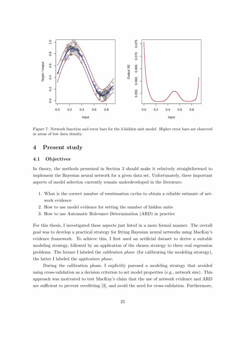
A plot of the network function is depicted in Figure 7, showing that the 3-hidden unit
model approximates the true data generating function well. Note that the Bayesian framework
also makes it possible to calculate ±1.96×SE bars on the network’s predictions. In Figure 7,
these error bars are represented by the red lines. In areas of high data density (corresponding
to the sections of curvature), the network error will typically be smaller. For this thesis,
however, I chose not to focus on issues related to the certainty of the network predictions.6
6Note that the R software written for this thesis does support the calculation of standard errors on networkpredictions
24
●
●
●● ●
●
●●
●●
●
●
●●
●
●●
●
●
●●
●●
●
●
●
●
●● ●
●
●●
●
●
●
●●
●
●
●
●
●
●
●
●
●
●
●●●●
●
●●
●
●
●●
●
●
●
●
●●
●
●●
●
●
●●
●
●●
●
●●
●
●
●
●
●
●●●
● ●●● ●●
●●
●
●
●●
●●
●●
●
●
●
●
●
●
●
●●
●●
●
●
●●
●
●●
●
●
●
●●
●
●
●●●●
● ●●
●
● ●
●
●●
●
●
●
●
●
●
●
●
●●● ●●●
●
●
●
●
● ●
●
●
●
●
●
●●
●●●
●
●●
●
●
●
●
●
●
●
●
●
●
●
●●●
●
●
●
●
●●
●
●
● ●
●
● ●
0.0 0.2 0.4 0.6 0.8
0.0
0.2
0.4
0.6
0.8
1.0
Input
Targ
et /
outp
ut
0.0 0.2 0.4 0.6 0.8
0.05
50.
060
0.06
50.
070
0.07
5
Input
Out
put S
EFigure 7: Network function and error bars for the 3-hidden unit model. Higher error bars are observedin areas of low data density.
4 Present study
4.1 Objectives
In theory, the methods presented in Section 3 should make it relatively straightforward to
implement the Bayesian neural network for a given data set. Unfortunately, three important
aspects of model selection currently remain underdeveloped in the literature:
1. What is the correct number of reestimation cycles to obtain a reliable estimate of net-
work evidence
2. How to use model evidence for setting the number of hidden units
3. How to use Automatic Relevance Determination (ARD) in practice
For this thesis, I investigated these aspects just listed in a more formal manner. The overall
goal was to develop a practical strategy for fitting Bayesian neural networks using MacKay’s
evidence framework. To achieve this, I first used an artificial dataset to derive a suitable
modeling strategy, followed by an application of the chosen strategy to three real regression
problems. The former I labeled the calibration phase (for calibrating the modeling strategy),
the latter I labeled the application phase.
During the calibration phase, I explicitly pursued a modeling strategy that avoided
using cross-validation as a decision criterion to set model properties (e.g., network size). This
approach was motivated to test MacKay’s claim that the use of network evidence and ARD
are sufficient to prevent overfitting [3], and avoid the need for cross-validation. Furthermore,
25

in many practical applications it will be of interest to avoid cross-validation, for instance when
the available training data are sparse.
In the application phase, performance of the Bayesian modeling strategies was compared
to a non-Bayesian strategy using ordinary neural networks and standard cross-validation.
Performance was measured by (a) generalization error (as measured on independent test
data) and (b) total computation time required for fitting models. Before further outlining
the method of this study, I specify the three problems listed above in more detail.
4.2 Problems of model selection
4.2.1 Number of reestimation cycles
An important open problem in the evidence framework concerns the number of reestimation
cycles required to obtain a stable estimate for the evidence. At present, there are no clear
guidelines as to how this number must be set, nor is it clear how the number of reestimation
cycles influences the final solution. Studies that apply Bayesian neural networks using the
evidence framework use arbitrary rules to decide the number of reestimation cycles, with
some using only 3 cycles [11, 15], 10 cycles [14], or until some ‘convergence’ criterion has
been satisfied [16]. Setting a fixed number of cycles seems the most practical solution from
a computational point of view. The drawback of this method is that we assume that any
network, regardless of the number of data points, input variables, or hidden units can be fitted
with the same number of reestimation cycles. If larger networks require more reestimation
cycles, setting the number of cycles too low may lead to a form of early stopping and produce
solutions that are not representative for that particular network size.
Reestimating parameters until a point of convergence has been reached seems more
correct from a mathematical point of view. Unfortunately, it is not clear whether a point
of convergence actually exists. Given the approximations of the evidence framework, data
that are poorly suited to the Gaussian assumptions may not converge to a stable solution at
all [11]. Furthermore, whether stable estimates for parameters can be obtained may depend
on the particular regularization scheme that is used (single versus multiple priors). For this
thesis, I looked more closely at how the number of reestimation cycles influences the final
evidence solution. In particular, I addressed the following questions:
• Does the evidence converge across the number of reestimation cycles?
• How does the number of reestimation cycles influence the relation between evidence and
test error?
• Is there an ideal number of reestimation cycles?
• Does the ideal number of reestimation cycles depend upon the dimensions of the net-
work?
26

4.2.2 Evidence as a model selection criterion
One of the advertised applications of model evidence is its strength to determine model perfor-
mance without the need for external validation data [7]. The literature cited in Section 3.4.3
casts doubt on this assertion, suggesting that evidence can be poorly related to generalization
error. For this thesis, I reexamined the utility of model evidence as a criterion for model
selection and/or network size selection. I inspected (a) whether network evidence is capable
of identifying an optimal network size and (b) how the correlation between model evidence
and test error (as measured on independent data) varies as a function of the number of rees-
timation cycles, the network size, the number of training data available, and the number of
irrelevant variables (probes) in the input data.
4.2.3 ARD pruning
The ARD prior described in Section 3.3.4 is motivated by the desire to determine variable
importance without resorting to cross-validation. In theory, the ARD model should auto-
matically shut off irrelevant variables during the reestimation process, therefore requiring
no variables to be dropped explicitly from the model. This strategy is called soft pruning.
Empirically, however, it has been found that dropping irrelevant variables from the predictor
set improves performance of the network [14]. Dropping variables based on the ARD results
is a strategy called hard pruning. Hard pruning requires additional decisions to be made,
such as the decay threshold for dropping a variable, and also which model to use for prun-
ing. Unfortunately, well-defined strategies for pruning variables using ARD have not been
formulated.
Intuitively, a model that has high evidence should also accurately reflect variable im-
portance, suggesting the following strategy for hard ARD pruning:
• Fit multiple networks of varying complexity
• Select the individual model with the highest evidence
• Inspect decay values for this model and drop variables with a decay value exceeding a
certain threshold
• Repeat the regular fitting process for the reduced data
An alternative strategy would be to prune variables based on multiple networks simultane-
ously, i.e. a so-called committee-based approach:
• Fit multiple networks of varying complexity
• Retain all networks of the optimal network size (as determined by evidence)
• Compute the median decay for each variable across the retained networks7
• Drop variables with a median decay value exceeding a certain threshold
7The median is preferred for robustness against outlying networks
27

• Repeat the regular fitting process for the reduced data
If we wish to avoid cross-validation then the pruning model should be chosen by its evidence.
For this thesis, I compared soft pruning with the two hard pruning strategies outlined above.
As a cut-off threshold for hard pruning, I chose log(α) > 1, which is slightly more liberal than
choosing log(α) > 0 (equal to α > 1, see Section 3.3.4)
5 Method
5.1 Calibration phase
In the calibration phase, I derived a general model fitting strategy for Bayesian neural net-
works using an artificial dataset. Data were generated from a linearly increasing sine wave
with added Gaussian noise:
Y = 100 sin(0.02X) + 0.5X + ε (40)
with ε drawn from N (0, 25), and X representing points 1 through 2000. The curvature in this
function should require at least some hidden units for correct modeling. From this function, I
sampled 2000 data points as a response variable. In addition, 9 randomly generated variables
were added to the input data which had no relation to the response variable, and functioned as
so-called probes. Each of these probes was generated from a uniform distribution, U (−1, 1).
For modeling, the following network settings were varied:
• Size of the training data set, Ntrain: 50, 250, or 1000 (remaining data are used as test
data)
• Size of the probe set, P : 0, 4, or 9
• Network size, H: 1 through 10 hidden units
• Number of reestimation cycles: 1 through 100 cycles
• Number of networks per setting: 20
Thus, 1800 different networks were fitted in total, each reestimated for 100 cycles. The 20
networks for each setting were initialized with different starting values for the weights. All
networks used the ARD prior to regularize the weights.
5.1.1 Convergence of network evidence
With regard to convergence, we are faced with three possibilities: (a) the network evidence
converges to a single value, (b) the network evidence fluctuates stably between different
values, (c) the network evidence fluctuates randomly between different values. Scenario (c)
would imply that the network parameters show no convergence at all. Scenario (a) is ideal
28

but may not be realistic in practice. Empirically, it has been found that network evidence
does not always converge to one value but stably fluctuates between several values. This is
likely a consequence of the Gaussian approximations in the evidence framework on one hand,
and the presence of multiple minima in the error function on the other hand.
Therefore, it may be misleading to use the raw sequence of evidences values to test con-
vergence. Instead, we can inspect the cumulative mean of the values across cycles rather than
the values themselves. For networks showing stable fluctuations between different evidence
values, the cumulative mean will show convergence whereas the raw values will not. As a
tolerance criterion, I chose a rather moderate threshold of 1 × 10⁻². In other words, if the
reduction in the cumulative mean of the evidence fell below a 1×10⁻² from the previous to the
next reestimation cycle, then convergence was satisfied. For networks showing no convergence
or convergence to infinite values, the convergence point was automatically set to infinity.
In order to inspect the relation between convergence point and model properties, I
regressed the reestimation cycle of convergence on network size (1 through 10), size of the
training set (50, 250, or 1000), and size of the probe set (0, 4, or 9). For this purpose, I used
a saturated model including all possible interactions and using only those networks which
showed convergence.
5.1.2 Evidence as a model selection criterion
To investigate the usefulness of model evidence as a selection criterion, I first inspected
boxplots of the evidence distribution for the fitted networks as a function of network size,
training set, and probe set (e.g., Figure 5). These plots should indicate whether, on average,
the evidence is capable of identifying the optimal network size. For this purpose, the optimal
network size was first determined by identifying the network size with the lowest test error
for the Ntrain = 1000, and P = 0 setup.8 Test error was calculated as the mean squared
prediction error on independent validation data drawn from the function defined in (40).
In addition, I inspected how the distribution of the evidence changed as a function of
the number of reestimation cycles. Because it was not possible to inspect boxplots for all
reestimation cycles, I focused only on the evidence distribution for 3, 10, 25, and 100 cycles.
These figures conformed to numbers of reestimation cycles used in earlier studies.
Secondly, I inspected how the (Pearson) correlation between model evidence and test
error varied as a function of the number of reestimation cycles, the network size, the number
of training data available, and the number of irrelevant variables (probes) in the input data.
5.1.3 Automatic Relevance Determination
To investigate the usefulness of Automatic Relevance Determination for the artificial data, I
first inspected whether the ARD prior was successful at identifying the irrelevant probes in
8The setup with the most training data available and no irrelevant noise variables.
29

the P = 9 setup (i.e., a soft pruning approach). Normally, irrelevant probes should acquire
large decay values (αk) during the reestimation process, while the relevant input variable
should acquire a small decay value. In particular, I compared three different approaches for
assessing variable importance:
• Inspecting decay values for the network with the highest evidence
• Inspecting decay values for the network with the lowest test error
• Inspecting median decay values for the optimal network size
The last approach is equivalent to a committee-based approach for assessing variable impor-
tance. The committee-based approach should tell whether, on average, the optimal network
size correctly estimates variable relevancies. In this case, the optimal network size was that
determined by (median) network evidence, as identified in the second part of the calibration
phase. Again, I preferred network evidence over test error in order to avoid cross-validation
whenever possible.
To identify irrelevant variables by their decay value, I utilized log decay plots, which
plot the logarithm of the decay values for each variable rather than the raw values themselves.
This ensured that variables with a decay value below 1 (little regularization) would have a log
decay value below 0, whereas variables with a decay value above 1 (increasing regularization),
would have a log decay value above 0, facilitating interpretation. Furthermore, it is often found
that decay values of irrelevant variables tend to grow extremely large. A log transformation
facilitates visual inspection of these values.
For the hard pruning strategy—which explicitly drops irrelevant variables from the
model—I simply contrasted the test errors obtained for the different probe sets, 9 versus
4 versus 0 probes. In addition, I inspected how these differences changed as a function of
training set.
All networks used during ARD inspection were derived from an optimal reestimation
cycle identified in the first part of the calibration phase. This approach was motivated by the
desire to keep computation time to a minimum when fitting Bayesian neural networks.
5.2 Application phase
All Bayesian neural networks in the application phase utilized the ARD prior to regularize
the weights (Section 3.3.4). For each dataset, I applied the modeling strategy derived during
the calibration phase, avoiding cross-validation to set model properties.
For ordinary neural networks, I used an internal K-fold cross-validation on the training
data to set the number of hidden units and the weight decay parameter. Values of K =
3, 5, and 10 were chosen for the Forest Fires data, Concrete Compressive Strength data,
and California Housing data, respectively.9 Network sizes 1 through 10 hidden units were
9Depending on the scarcity of the available training data
30

considered, and decay values (0, 0.0001, 0.001, 0.01, 0.1, 1, 10).10 Once the optimal network
settings were identified, this model was reestimated three times with different starting values
for the weights and applied to the independent test data. This I did to prevent the possibility
of accidentally obtaining a local minimum solution as the final network.
Performance for Bayesian and non-Bayesian networks was compared by (a) predictive
accuracy on the test data, as measured by mean squared prediction error (MSPE), and (b)
total computation time required in minutes.
5.2.1 Forest Fires data
The Forest Fires dataset [17] contains data about the size of forest fires in the Montesinho nat-
ural park in Portugal, and is available from the UCI Machine Learning repository.11 Cortez
and Morais [17] used linear regression, decision trees, neural networks, support vector ma-
chines, and random forests to predict the area of burned surface based on meteorological and
geographical predictors (see Table 1). Because the distribution of the response variable is
extremely right skewed, Cortez and Morais chose to model log(area+ 1) rather than the raw
area of burned surface.
Variable Type Description
X Continuous x-axis coordinate (from 1 to 9)Y Continuous y-axis coordinate (from 1 to 9)month Categorical Month of the year (January to December)day Categorical Day of the week (Monday to Sunday)
FFMC Continuous Fine fuel moisture codeDMC Continuous Duff moisture codeDC Continuous Drought codeISI Continuous Initial spread index
temp Continuous Outside temperature (in ◦C)RH Continuous Outside relative humidity (in %)wind Continuous Outside wind speed (in km/h)rain Continuous Outside rain (in mm/m2)
area Continuous Total burned area (in ha)
Table 1: List of variables in the Forest Fires dataset (Ntotal = 513).
For this thesis, I modeled the log-transformed area of burned surface as a function of the
12 predictor variables. Note that both month and day are categorical variables, necessitating
the construction of indicator variables to code for individual factor levels. This expanded the
original input data to 24 predictors in total. Prior to modeling, all cases for the months of
january, may, and november were dropped from the data due to the low sampling frequency
10Corresponding to log(α) values (NA,−9.210,−6.908,−4.605,−2.303, 0, 2.303)11http://archive.ics.uci.edu/ml/datasets/Forest+Fires
31

(5 cases). Continuous predictor variables were scaled and the data were then randomly split
into a training set (Ntrain = 256) and a test set (Ntest = 257).
log( Area of Burned Surface + 1 )
Den
sity
0 1 2 3 4 5 6 7
0.0
0.2
0.4
0.6
0.8
1.0
Figure 8: Density of log transformed area of burned surface.
5.2.2 Concrete Compressive Strength data
The Concrete Compressive Strength data [18] contains info on the characteristics of concrete,
and is available from the UCI Machine Learning repository.12 The compressive strength of
concrete (measured in megapascals) is known to be a highly nonlinear function of age and
ingredients (see Table 2).
Variable Type Unit of measurement
cement Continuous kg in a m3 mixtureblast furnace slag Continuous kg in a m3 mixturefly ash Continuous kg in a m3 mixturewater Continuous kg in a m3 mixturesuperplasticizer Continuous kg in a m3 mixturecoarse aggregate Continuous kg in a m3 mixturefine aggregate Continuous kg in a m3 mixtureage Continuous Day (1–356)
compressive strength Continuous MPa
Table 2: List of variables in the Concrete Compressive Strength dataset (Ntotal = 1030).
For this thesis, I modeled concrete compressive strength as a function of the 8 predictor
variables. Prior to modeling, all variables were scaled and the data were randomly split into
a training set (Ntrain = 515) and a test set (Ntest = 515).
12http://archive.ics.uci.edu/ml/datasets/Concrete+Compressive+Strength
32

Concrete Compressive Strength
Den
sity
−2 −1 0 1 2 3
0.0
0.1
0.2
0.3
0.4
Figure 9: Density of concrete compressive strength.
5.2.3 California Housing data
The California Housing data [19] contains aggregated information on median house value in
20,460 neighborhoods in California (1990 census data), and is available from the Carnegie-
Mellon StatLib repository.13 The goal of these data is to model the median house value as a
function of neighborhood demographics and house characteristics, such as housing density or
average number of rooms (Table 3). Hastie and colleagues [1] used gradient boosted regression
trees on these data and identified interaction effects between the number of households and
median house age, as well as between longitude and latitude, to predict median house value.
Variable Type Description
median income Continuous Median income in neighborhoodmedian house age Continuous Median house age in years in neighborhoodtotal rooms Continuous Total number of rooms in neighborhoodtotal bedrooms Continuous Total number of bedrooms in neighborhoodpopulation Continuous Number of residents in neighborhoodhouseholds Continuous Number of households in neighborhoodlatitude Continuous Latitude of neighborhoodlongitude Continuous Longitude of neighborhood
median house value Continuous Median house value in units of $100,000 in neighborhood
Table 3: List of variables in the California Housing dataset (Ntotal = 20, 460). Note that individualobservations denote neighborhoods in this dataset.
For this thesis, I modeled median house value as a function of the 8 predictor variables.
Prior to modeling, all variables were scaled and the data were randomly split into a training
13http://lib.stat.cmu.edu/datasets/
33

set (Ntrain = 5000) and a test set (Ntest = 15, 460).
Median House Value
Den
sity
0e+00 1e+05 2e+05 3e+05 4e+05 5e+05
0e+
001e
−06
2e−
063e
−06
4e−
06
Figure 10: Density of median house value.
5.3 Software
At present, no packages implementing Bayesian neural networks are available in R. Therefore,
a custom library was written (R version 2.12.2, 64-bit) to implement Bayesian neural networks
for regression. This library consists of a main neural network function, called bfnn, and several
auxiliary functions to plot network results. The appendix contains a detailed list of required
packages to run bfnn, and a description of control arguments.
Once the network settings have been initialized by bfnn, the algorithm proceeds in
the manner described in Section 3.5, including the computational addenda described in Sec-
tion 3.4.
To contrast performance of the Bayesian neural network to the standard feedforward
neural network in this thesis, a custom R function called bfnn.FNN was written to implement
the standard network. Here, I chose not to use the nnet function from the base expansion due
to the fact that nnet relies on optim for optimization, whereas bfnn uses the more efficient
ucminf function. The custom function makes bfnn.FNN as similar to bfnn as possible.
Tracking of the computation time required to carry out calculations for the three regres-
sion problems was achieved through R’s base system.time function.
34

6 Results
6.1 Calibration phase
6.1.1 Convergence of network evidence
The left panel of Figure 11 shows the median point of convergence of the network evidence
for a given network size, training set, and probe set. The right panel of Figure 11 shows
the fraction of networks that did not converge (i.e., convergence set to infinity) for a given
network size, training set, and probe set. From these plots, it is apparent that for many
combinations of settings, few or even none of the networks showed convergence. The total
fraction of networks that did show convergence was 22.3%. The right panel of Figure 11
suggests that network size is the most important determinant for convergence, with larger
networks less likely to converge. As pointed out before, this is likely a consequence of the
Gaussian approximations in the evidence framework on one hand, and the presence of multiple
minima on the other hand.14
●
●
●
●
●
●
●
●
2040
6080
Network size
Med
ian
rees
timat
ion
cycl
e of
con
verg
ence
●
●
●
●
●
●
●
●
1 2 3 4 5 6 7 8 9 10
● ● ●N50 P0N250 P0N1000 P0
N50 P4N250 P4N1000 P4
N50 P9N250 P9N1000 P9
●
●
●
●
●
● ●
● ●
●
0.0
0.2
0.4
0.6
0.8
1.0
Network size
Fra
ctio
n of
non
−co
nver
ged
netw
orks
●
●
● ●
●
●
●
●
● ●●
●
●
●
●
● ● ● ● ●
1 2 3 4 5 6 7 8 9 10
● ● ●N50 P0N250 P0N1000 P0
N50 P4N250 P4N1000 P4
N50 P9N250 P9N1000 P9
Figure 11: Left panel: Median reestimation cycle of convergence for network evidence. Right panel:fraction of networks that did not converge. N = size of training set, P = size of probe set.
A linear regression was carried out for the converged networks regressing reestimation
cycle of convergence on network size (1 through 10), size of the training set (50, 250, or 1000),
and size of the probe set (0, 4, or 9). Results of this regression are summarized in Table 4.
As expected, network size has the largest influence on the convergence point, followed by the
number of probes. In general, having more hidden units and more input variables necessitates
more reestimation cycles, although there is an interference interaction between these two
predictors that dampens this number when both network size and input size increase. The
14Note also that the current software makes computational adjustments that may alter the course of thereestimation process.
35

size of the training set seems to have little effect on the number of reestimation cycles, even in
interactions. Caution is warranted with interpreting these trends, however, due to the overall
low number of converging networks.
Coefficient Estimate 95% CI t-value p-value
(Intercept) 11.648 [4.57,18.72] 3.24 0.001Network size 6.908 [5.25,8.75] 8.18 < 0.001Training set -0.000 [-0.01,0.01] -0.05 0.960Probe set 8.490 [6.41,10.57] 8.04 < 0.001
Network size × Training set 0.002 [-0.01,0.01] 0.79 0.432Network size × Probe set -1.747 [-2.09,-1.40] -10.00 < 0.001Training set × Probe set -0.005 [-0.02,-0.01] -2.87 0.004
Network size × Training set × Probe set 0.001 [0.00,0.00] 1.86 0.064
Table 4: Relation between the mean point of convergence and network properties.
The model in Table 4 allows us to estimate a minimum required number of reestimation
cycles for the lowest network settings. For a network with only 1 input variable (0 probes),
1 hidden unit, and 50 available training cases, at least 25 reestimation cycles are necessary
for convergence. Even for this simple dataset, 25 reestimation cycles is considerably higher
than the numbers employed in studies by Nguyen (3 reestimation cycles, [15]) and Penny and
Roberts (10 reestimation cycles, [14]). Furthermore, it is clear that this number should be
adapted based on the network properties, rather than be kept fixed. The model estimated
in Table 4 may have limited utility to set the number of reestimation cycles, however, as for
certain combinations of network settings it may predict a very low or even negative number of
reestimation cycles. In general, the best strategy is probably to use a small linear increase in
reestimation cycles as the network becomes more complex (more hidden units and/or input
variables).
Finally, it was found during calibration that, for networks where the number of pa-
rameters exceeded the number of data points (e.g., size = 5, P = 9, for Ntrain = 50), the
evidence automatically dropped to minus infinity after two or three reestimation cycles. In
other words, in the current implementation, network evidence cannot be reliably used when
the number of parameters exceeds the number of data points, severely limiting its usefulness
in that area.
6.1.2 Evidence as a model selection criterion
The optimal network size for these data was first determined by identifying the network size
with the lowest median test error for the Ntrain = 1000, and P = 0 setup. Figure 12 plots the
distribution of the mean squared prediction error on the test data as a function of network
size (at reestimation cycle 100). From this plot, it is clear that the 3-hidden unit architecture
36

is the optimal network size for these data, although the difference with the 4-hidden unit
structure is negligible.
●
● ●● ●
1 2 3 4 5 6 7 8 9 10
0.00
0.05
0.10
0.15
0.20
0.25
0.30
N=1000, P=0
Network size
Mea
n sq
uare
d pr
edic
tion
erro
r
Figure 12: Distribution of network evidence as a function of network size at reestimation cycle 100.
Figures 13 through 16 show how the distribution of network evidence evolves between 3,
10, 25 and 100 reestimation cycles for varying levels of network size, training set, and probe
set. Before looking more closely at this evolution, however, it is instructive to inspect the
distribution of evidence for the case Ntrain = 1000, P = 0, at the 100th cycle (Figure 16,
top right panel). When training data are abundant and no additional noise is added by
random probes, the highest median evidence is achieved for the 3-hidden unit network, again
suggesting that this is the optimal network architecture for these data. As with the test error,
the 3-hidden unit network is in close competition with the 4-hidden unit network, however,
often producing median evidence that is comparable or higher than the 3-hidden unit network.
This is particularly the case when the number of irrelevant probes increases (Figure 16, center
right and bottom right panel).
From Figure 16, we also see that the distribution of the evidence tends to become wider
for increasing network sizes. For the 1- and 2-hidden unit networks, there is almost no
variation in the evidence, whereas for the 10-hidden unit network there is much variation.
This wide distribution likely reflects the increasing number of local minima for this network
size.
If we inspect the evolution of the evidence across reestimation cycles, two general con-
clusions can be drawn. Firstly, larger networks take more reestimation cycles to achieve stable
evidence estimates. At the 3rd reestimation cycle, the median evidence for many of the larger
networks is still below zero, and far below that of the smaller networks. At the 25th rees-
37

●●●
●
●
●●●
●
●●●●
●
●
●
●
1 2 3 4 5 6 7 8 9 10
−10
00−
800
−60
0−
400
−20
00
N=50, P=0
●●
●
●
●
●
●
●
●
1 2 3 4 5 6 7 8 9 10
−60
0−
400
−20
00
N=250, P=0
●
●
●●
●
●
●
1 2 3 4 5 6 7 8 9 10
300
400
500
600
700
800 N=1000, P=0
●
●
●
●
●●
●
●
●
●
●
●
●●
1 2 3 4 5 6 7 8
−15
00−
1000
−50
00
N=50, P=4
1 2 3 4 5 6 7 8 9 10
●●
●●
●●
●
●
●
●
●
1 2 3 4 5 6 7 8 9 10
−50
00−
3000
−10
000
N=250, P=4
●
●
●
●
●●●
● ●
●
●
●
●
●
●
●
1 2 3 4 5 6 7 8 9 10
−20
00−
1000
050
015
00
N=1000, P=4
●●●●
●●
●
●
●
●
●
1 2 3 4 5
−60
00−
4000
−20
000
N=50, P=9
1 2 3 4 5 6 7 8 9 10
●●
●●
●
●
●
●
●
●
●
●
1 2 3 4 5 6 7 8 9 10
−10
000
−50
000
N=250, P=9
●
●
●●
1 2 3 4 5 6 7 8 9 10
−40
00−
2000
020
00
N=1000, P=9
Figure 13: Distribution of network evidence (y-axis) as a function of network size (x-axis), trainingset (N), and probe set (P ), at reestimation cycle 3.
38

●
●
●●
1 2 3 4 5 6 7 8 9 10
−10
00−
800
−60
0−
400
−20
00
N=50, P=0
●● ●
●
●
●
●
1 2 3 4 5 6 7 8 9 10
−80
0−
600
−40
0−
200
0
N=250, P=0
●
●●●
1 2 3 4 5 6 7 8 9 10
−20
00
200
400
600
800
N=1000, P=0
●
●●●
●
●
●
●
1 2 3 4 5 6 7 8
−25
00−
1500
−50
00
500
N=50, P=4
1 2 3 4 5 6 7 8 9 10
●●●●●●
●
●
●
●
●
●
●
1 2 3 4 5 6 7 8 9 10
−50
00−
3000
−10
000
1000
N=250, P=4
●
●
●
1 2 3 4 5 6 7 8 9 10
−20
00−
1000
010
00
N=1000, P=4
●
●
●
●
●
●
●
●
●
●
●
1 2 3 4
−10
000
500
1000
2000
N=50, P=9
1 2 3 4 5 6 7 8 9 10
●
●●
●
●
●
●
1 2 3 4 5 6 7 8 9 10
−10
000
−50
000
N=250, P=9
●●
●●
●
1 2 3 4 5 6 7 8 9 10
−80
00−
4000
020
00
N=1000, P=9
Figure 14: Distribution of network evidence (y-axis) as a function of network size (x-axis), trainingset (N), and probe set (P ), at reestimation cycle 10.
39

●●●
●
●
●
●
●
1 2 3 4 5 6 7 8 9 10
−10
00−
800
−60
0−
400
−20
00
N=50, P=0
●●
●
●
●●
●
●●
●
●
●●●
●
1 2 3 4 5 6 7 8 9 10
−60
0−
400
−20
00
N=250, P=0
●
●
●
●
1 2 3 4 5 6 7 8 9 10
−20
00
200
400
600
800
N=1000, P=0
●
●
●●
●
●
1 2 3 4 5 6 7 8
−15
00−
1000
−50
00
500
N=50, P=4
1 2 3 4 5 6 7 8 9 10
●●
●
1 2 3 4 5 6 7 8 9 10
−30
00−
2000
−10
000
1000
N=250, P=4
●
●●
1 2 3 4 5 6 7 8 9 10
−30
00−
2000
−10
000
1000
N=1000, P=4
●
●
●
●
1 2 3 4
−10
000
1000
2000
N=50, P=9
1 2 3 4 5 6 7 8 9 10
●
●
●
●
●
●
●
1 2 3 4 5 6 7 8 9 10
−10
000
−60
00−
2000
020
00
N=250, P=9
●●●
●
1 2 3 4 5 6 7 8 9 10
−10
000
−60
00−
2000
020
00
N=1000, P=9
Figure 15: Distribution of network evidence (y-axis) as a function of network size (x-axis), trainingset (N), and probe set (P ), at reestimation cycle 25.
40

●
●●
●
●
●
●
●
●
1 2 3 4 5 6 7 8 9 10
−80
0−
600
−40
0−
200
0
N=50, P=0
●●
●
●
●
●
●●
●●
●
●
●
●
●
●
●
●
1 2 3 4 5 6 7 8 9 10
−60
0−
400
−20
00
N=250, P=0
●
●
●
●
●●
●
●
●
●
●
1 2 3 4 5 6 7 8 9 10
−20
00
200
400
600
800
N=1000, P=0
●●●
●
●
●
●●●
●
●
●
1 2 3 4 5 6 7
−20
00−
1500
−10
00−
500
050
0
N=50, P=4
1 2 3 4 5 6 7 8 9 10
●
●
●
1 2 3 4 5 6 7 8 9 10
−30
00−
2000
−10
000
1000
N=250, P=4
●
●
●●●
●
●●
1 2 3 4 5 6 7 8 9 10
−30
00−
2000
−10
000
1000
N=1000, P=4
●
●
1 2 3 4
−20
00−
1000
010
0020
00
N=50, P=9
1 2 3 4 5 6 7 8 9 10
●
●
● ●
●
●
●
1 2 3 4 5 6 7 8 9 10
−10
000
−60
00−
2000
020
00
N=250, P=9
●
●
●
1 2 3 4 5 6 7 8 9 10
−10
000
−60
00−
2000
020
00
N=1000, P=9
Figure 16: Distribution of network evidence (y-axis) as a function of network size (x-axis), trainingset (N), and probe set (P ), at reestimation cycle 100.
41

timation cycle, the difference with the 100th reestimation cycle is not that large anymore.
Secondly, the number of probes influences how quickly the correct model can be identified by
network evidence. For 9 probes, the 1- and 2-hidden unit networks are still identified as the
best networks at the 3rd reestimation cycle (Figure 13, bottom panels). It is not until after
the 10th reestimation cycle that the 3- and 4-hidden unit networks are identified as the best
models.
Next, I examined the correlation between network evidence and test error. Figure 17
plots the cumulative mean of these correlations across the 100 reestimation cycles for each
a given network size, training set, and probe set. The curves of interest on these plots are
those of the 3-hidden unit network (dark blue) and the 4-hidden unit network (light blue).
Overall, it appears that, for these networks, the correlation between network evidence and
test error is consistently the lowest. After 100 reestimation cycles, the average correlation
between network evidence and test error is far below 0, as expected. For all networks, this
correlation generally tends to remain below zero, but for the less likely networks (in terms of
their evidence), the average correlation tends to fluctuate near zero. In most cases, the average
correlation stabilizes around the 25th or 30th reestimation cycle. This finding reconfirms the
result that 25 reestimation cycles are a minimum to obtain stable network evidence.
Overall, it appears that the evidence is successful at identifying an optimal network size.
Furthermore, the (negative) correlation between evidence and test error also tends to be the
strongest for networks of the optimal size. This result is extremely useful for applications
using ARD, as shall be shown in the next paragraph.
6.1.3 Automatic Relevance Determination
Figure 18 compares the different strategies for determining variable relevance with the ARD
prior when Ntrain = 1000. This time, I obtained values from networks at the 30th reestimation
cycle, which my previous results have shown to be a reasonable minimum. The top left panel
of Figure 18 clearly shows that the model with the highest evidence correctly estimated high
decay values for the 9 irrelevant probe variables, and low decay values for the relevant input
variable (X) and the hidden units. Although the logarithm of the X variable’s decay value
is slightly above zero, it is still below my nominal cutoff of 1. Nearly identical results were
obtained for the network showing the lowest test error, which was a 3-hidden unit network
in this case. As expected, the model with the lowest evidence (Figure 18, bottom left panel)
also failed to identify the irrelevant probes in the input set, with all variables in this model
having a log transformed decay value below zero.
Next, I looked at the distribution of the (log transformed) decay values for the optimal
network architecture as identified by the network evidence (committee-based assessment).
For the setting Ntrain = 1000, P = 0, this was the 4-hidden unit model. The bottom right
panel of Figure 18 shows that the median log decay value for the bias unit, the X variable
42

1
111111111111111111111111111111111111111111111111111111111111111111111111111111111111111111111111111
0 20 40 60 80 100
−1.
0−
0.5
0.0
0.5
1.0
N=50, P=0
Reestimation cycle
cor(
evid
ence
,test
err
or)
2222222222222222222222222222222222222222222222222222222222222222222222222222222222222222222222222222
333333333
333333333333333333
3333333333333333333333333333333333333333333333333333333333333333333333333
4
4444444
44444444444444444444444444444444444444444444444444444444444444444444444444444444444444444444
5
5555555555555555555555555555555555555555555555555555555555555555555555555555555555555555555555555556
66666
6666666666666666666666666666666666666666666666666666666666666666666666666666666666666666666666
7
77777
7777777777777777777777777777777777777777777777777777777777777777777777777777777777777777777777
8
8888888
88888888888888888888888888888888888888888888888888888888888888888888888888888888888888888888
9
99999999999
999999999999999999999999999999999999999999999999999999999999999999999999999999999999999911
11111111111111111111111111111111111111111111111111111111111111111111111111111111111111111111111111
1
111111111111111111111111111111111111111111111111111111111111111111111111111111111111111111111111111
0 20 40 60 80 100
−1.
0−
0.5
0.0
0.5
1.0
N=250, P=0
Reestimation cycle
cor(
evid
ence
,test
err
or)
2222222222222222222222222222222222222222222222222222222222222222222222222222222222222222222222222222
3333333333333333333333333333333333333333333333333333333333333333333333333333333333333333333333333333
4444
444444444444444444444444444444444444444444444444444444444444444444444444444444444444444444444444
5
55555
555555555555555555555555555555555555555555555555
55555555555555555555555555555555555555555555556666666666666666666666666666666666666666666666666666666666666666666666666666666666666666666666666666
7
777777777777777777777777777777
777777777777777777777777777777777777777777777777777777777777777777777
8888888888888888888888888888888888888888888888888888888888888888888888888888888888888888888888888888
9
9999
9999999999999999999999999999999999999999999999999999999999999999999999999999999999999999999999911
11111
111111111111111111111111111111111111111111111111111111111111111111111111111111111111111111111
1111111111111111111111111111111111111111111111111111111111111111111111111111111111111111111111111111
0 20 40 60 80 100
−1.
0−
0.5
0.0
0.5
1.0
N=1000, P=0
Reestimation cycle
cor(
evid
ence
,test
err
or)
22222222222222222222222222222222222222222222222222222222222222222222222222222222222222222222222222223333333333333333333333333333333333333333333333333333333333333333333333333333333333333333333333333333
4
444444
44444444444444
4444444444444444444444444444444444444444444444444444444444444444444444444444444
5555555555555555555555555555555555555555555555555555555555555555555555555555555555555555555555555555
66666666
66666666666666666666666666666666666666666666666666666666666666666666666666666666666666666666
7
77
77777777
777777777777777777777
77777777777777777777777777777777777777777777777777777777777777777777
8
8
8
88888888888888
88888888888888888888888888888888888888888888888888888888888888888888888888888888888
999
99999999
9999999
9999999999999999999999999999999999999999999999999999999999999999999999999999999999
1
11
111111111111
1111111111111111111111111111111111111111111111111111111111111111111111111111111111111
1
1
111111111
1111111
1111111111111111111
111111111111111111111
111111111111111111111111111111111111111111
0 20 40 60 80 100
−1.
0−
0.5
0.0
0.5
1.0
N=50, P=4
Reestimation cycle
cor(
evid
ence
,test
err
or)
2
2222222222222
2222222222222222222
22222222222222222222222222222222222222222222222222222222222222222223
333333
33333333333333333333333333333333333333333333333333333333333
3333333333333333333333333333333333444444444444
4444444444444444444444444444444444444444444444444444444444444444444444444444444444444444
55555555555555555555555555555555555555555555555555555555555555555555555555555555555555555555555555556
6
666666666666666666
66666666666666666666666666666666666666666666666666666666666666666666666666666666
7
777777777777777777777777
777777777777777777777777777777777777777777777777777777777777777777777777777
888
8888
88888888888888888888888888888888888888888888888888888888888888888888888888888888888888888888
9
1 11
11
1
1111111111111
1111111111111111111111111111111111111111111111111111111111111111111111111111111111
0 20 40 60 80 100
−1.
0−
0.5
0.0
0.5
1.0
N=250, P=4
Reestimation cycle
cor(
evid
ence
,test
err
or)
22222222
22222222222
222222222222222222222222222222222222222222222222222222222222222222222222222222222
33333333333333333
33333333333333333333333333333333333333333333333333333333333333333333333333333333333
4444444444444444444444444444444444444444444444444444444444444444444444444444444444444444444444444444
5555555555555555555555555555555555555555555555555555555555555555555555555555555555555555555555555555
6
6666666
66666666666666666666666666666666666666666666666666666666666666666666666666666666666666666666
7777777777777777777777777777777777777777777777777777777777777777777777777777777777777777777777777777
8888888888888888888888888888888888888888888888888888888888888888888888888888888888888888888888888888
9999999999999999999999999999999999999999999999999999999999999999999999999999999999999999999999999999
111111111111111111
11111111111111111111111111111
11111111111111111111111111111111111111111111111111111
11
1111
11111
11111111111
1111111111
11111111111111111111111
111111111111111111111111111111111111111111111
0 20 40 60 80 100
−1.
0−
0.5
0.0
0.5
1.0
N=1000, P=4
Reestimation cycle
cor(
evid
ence
,test
err
or)
2222222222222222
22222222
22222222222222222
2222222222222222222222222222222222222222222
2222222222222222
33333333333333333333333333
33333333333333333333333333333333333333333333333333333333333333333333333333
4444444444444444444444444444444444444444444444444444444444444444444444444444444444444444444444444444
5555555555555555555555555555555555555555555555555555555555555555555555555555555555555555555555555555
6
6666666666666666666666666666666666666666666666666666666666666666666666666666666666666666666666666667
777777777777777777777777777777777777777777777777777777777777777777777777777777777777777777777777777
8888888888888888888888888888888888888888888888888888888888888888888888888888888888888888888888888888
9
9
9999
99999999
99999999999999999999999999999999999999999999999999999999999999999999999999999999999999111111111
1111111111111111111111111111111111111111111111111111111111111111111111111111111111111111111
1111
1111111111111
11111
1111111111111111
11111111111111111111111111111111111
111111111111111111111111111
0 20 40 60 80 100
−1.
0−
0.5
0.0
0.5
1.0
N=50, P=9
Reestimation cycle
cor(
evid
ence
,test
err
or)
22222222
2222222222
2222222222222222222222222222222222222222222222222222222222222222222222222222222222
3
3
33333333333333333333333333333333333333333333333333333333
333333333333333333333333333333333333333333
444444444444444444444444
4444444444444444444444444444444444444444444444444444444444444444444444444444
5
55
6
7
8
9
1
1111
1
11111111111111111111111111111111111111111111111111111111111111111111111111111111111111111111111
0 20 40 60 80 100
−1.
0−
0.5
0.0
0.5
1.0
N=250, P=9
Reestimation cycle
cor(
evid
ence
,test
err
or)
2222222222222
222222222
22222222222
222222222222222222222222222222222222222222
2222222222222222222222222
3
3
33333333333333333333333333333333333333333333333333333333333333333333333333333333333333333333333333
4444444444444444444444444444444444444444444444444444444444444444444444444444444444444444444444444444
55
55555555555555555555555555555555555555555555555555555555555555555555555555555555555555555555555555
6666666666666666666666666666666666666666666666666666666666666666666666666666666666666666666666666666
7
777777777777777777777777777777777777777777777777777777777777777777777777777777777777777777777777777
8888888888888888888888888888888888888888888888888888888888888888888888888888888888888888888888888888
9999999999999999999999999999999999999999999999999999999999999999999999999999999999999999999999999999
1
111111111111111111111111111111111111111111111111111111111111111111111111111111111111111111111111111
11
1111
111111
111111111
111111111111111111111111
1111111111111111111111111111111111111111111111111111111
0 20 40 60 80 100
−1.
0−
0.5
0.0
0.5
1.0
N=1000, P=9
Reestimation cycle
cor(
evid
ence
,test
err
or)
222222222222222
2222222222222222222222222
222222222222222222222222222222222222222222222222222222222222
333333333333333333
3333333333333333333333333333333333333333333333333333333333333333333333333333333333
4
4444444444444444444444444444444444444444444
44444444444444444444444444444444444444444444444444444444
5555555555555555555555555555555555555555555555555555555555555555555555555555555555555555555555555555
6
666666666666666666666666666666666666666666666666666666666666666666666666666666666666666666666666666
7
77777777777777777777777777777777777777777777777777777777777777777777777777
7777777777777777777777777
8888888888888888888888888888888888888888888888888888888888888888888888888888888888888888888888888888
9
9
999999
99999999999999999999
999999999999999999999999999999999999999999999999999999999999999999999999
1
1
11111111111111111111111111111111111111111111111111111111111111111111111111111111111111111111111111
Figure 17: Cumulative mean of the correlation between network evidence and test error as a functionof reestimation cycle, training set (N), and probe set (P ). Colored numbers correspond to networksize (1 through 10), with the optimal 3- and 4-hidden unit networks in dark blue and light blue,respectively.
43

and the hidden units remains below the cutoff of 1 (red line). Furthermore, the distribution
of these decay values tends to be very narrow. For the irrelevant probes, all but one probe
have a median decay value far above the cutoff of 1. Probe 9 stays below the cutoff value
but has a wide distribution of decay values, as indeed most of the probes have. This result
suggests that irrelevant variables tend to exhibit more fluctuations in decay values.
Figure 19 compares the different strategies for determining variable relevance with the
ARD prior when Ntrain = 250. This time the highest evidence network had more difficulties
in identifying the irrelevant variables. In fact, the decay values of probes 3, 4, and 9 are even
lower than that of the X variable. The same is true for the network with the lowest test
error, which incorrectly identified probes 6 and 8 as relevant predictors. For the setup with
Ntrain = 250, more useful information is gained from the committee-based approach. The
distribution plot shows that the median log decay value for the bias, the X variable, and the
hidden units remains below the nominal cutoff value of 1. For the probes, all median log
decay values are well above this cutoff. Again, we see that the distribution of the log decay
values is much wider for the probes than for the relevant variables.
Based on these results, it would seem that a committee-based approach yields the most
useful information on variable relevance. Unfortunately, for the setup with Ntrain = 1000,
the committee-based approach failed to identify probe 9 as irrelevant. In this case, it may be
informative to also take into account measures of spread, such as the variance of the decay
values or the interquartile distance. For irrelevant variables, these values should be much
higher for relevant variables.
Finally, I inspected the usefulness of a hard pruning strategy by comparing the average
test error of networks with different probe sets. Table 5 gives the median test error as a
function of network size, training set, and probe set. The lowest test error for a given training
set size is always achieved for input data with 0 probes (grey cells). In other words, pruning
irrelevant variables from the input data always improves performance. Nevertheless, the gains
in test error appear to be minimal. As is clear from Table 5, a more important determinant
of the test error is the choice of network size, rather than the number of irrelevant variables.
Hard pruning also has important consequences for how network evidence should be
employed to determine the optimal network size. Recall from Figure 16 that, for the setup
with Ntrain = 1000, P = 9, network evidence mistakenly identified the 4-hidden unit network
as the optimal architecture. For the setup with Ntrain = 1000, P = 0, by contrast, network
evidence correctly identified the 3-hidden unit network as the optimal architecture. This
result suggests that, after hard pruning, all networks should be refitted to re-evaluate the
optimal network architecture.
44

bias X
Pro
be.1
Pro
be.2
Pro
be.3
Pro
be.4
Pro
be.5
Pro
be.6
Pro
be.7
Pro
be.8
Pro
be.9
Hid
den
Log(
deca
y)
−5
05
1015
2025
Maximum evidence, N=1000, H=4
bias X
Pro
be.1
Pro
be.2
Pro
be.3
Pro
be.4
Pro
be.5
Pro
be.6
Pro
be.7
Pro
be.8
Pro
be.9
Hid
den
Log(
deca
y)
−5
05
1015
2025
Minimum test error, N=1000, H=3
bias X
Pro
be.1
Pro
be.2
Pro
be.3
Pro
be.4
Pro
be.5
Pro
be.6
Pro
be.7
Pro
be.8
Pro
be.9
Hid
den
Log(
deca
y)
−20
−15
−10
−5
0
Minimum evidence, N=1000, H=10
●
●
●
●
●
●
●
●
●
●
●
●
●
●
●
●
●
●
●
●
●●
●
●−10
010
20
Decay distribution for N=1000, H=4
Log(
deca
y)
bias X
Pro
be.1
Pro
be.2
Pro
be.3
Pro
be.4
Pro
be.5
Pro
be.6
Pro
be.7
Pro
be.8
Pro
be.9
Hid
den
Figure 18: Automatic Relevance Determination. Top left: decay values for the model with the highestevidence. Top right: decay values for the model with the minimum test error. Bottom left: decayvalues for the model with the lowest evidence. Bottom right: distribution of decay values for theoptimal network structure of 4 hidden units. All models were derived from the 30th reestimationcycle, with Ntrain = 1000.
45

bias X
Pro
be.1
Pro
be.2
Pro
be.3
Pro
be.4
Pro
be.5
Pro
be.6
Pro
be.7
Pro
be.8
Pro
be.9
Hid
den
Log(
deca
y)
−10
−5
05
1015
2025
Maximum evidence, N=250, H=4
bias X
Pro
be.1
Pro
be.2
Pro
be.3
Pro
be.4
Pro
be.5
Pro
be.6
Pro
be.7
Pro
be.8
Pro
be.9
Hid
den
Log(
deca
y)
−5
05
1015
2025
Minimum test error, N=250, H=3bi
as X
Pro
be.1
Pro
be.2
Pro
be.3
Pro
be.4
Pro
be.5
Pro
be.6
Pro
be.7
Pro
be.8
Pro
be.9
Hid
den
Log(
deca
y)
−20
−15
−10
−5
0
Minimum evidence, N=250, H=9
●
●
●
●
●●
●●
●●
●●
●
−20
−10
010
20
Decay distribution for N=250, H=4
Log(
deca
y)
bias X
Pro
be.1
Pro
be.2
Pro
be.3
Pro
be.4
Pro
be.5
Pro
be.6
Pro
be.7
Pro
be.8
Pro
be.9
Hid
den
Figure 19: Automatic Relevance Determination. Top left: decay values for the model with the highestevidence. Top right: decay values for the model with the minimum test error. Bottom left: decayvalues for the model with the lowest evidence. Bottom right: distribution of decay values for theoptimal network structure of 4 hidden units. All models were derived from the 30th reestimationcycle,with Ntrain = 250.
46

Network size (H)Training set (N) Probe set (P ) 1 2 3 4 5 6 7 8 9 10
50 0 0.228 0.148 0.075 0.074 0.074 0.074 0.083 0.075 0.075 0.0884 0.230 0.155 0.098 0.133 0.183 0.439 0.821 0.886 0.650 0.5459 0.245 0.163 0.560 1.089 1.103 0.559 0.580 0.546 0.516 0.540
250 0 0.225 0.154 0.068 0.070 0.070 0.072 0.072 0.072 0.072 0.0724 0.221 0.150 0.074 0.076 0.080 0.084 0.097 0.097 0.109 0.1179 0.221 0.153 0.077 0.082 0.095 0.098 0.134 0.150 0.172 0.218
1000 0 0.221 0.144 0.067 0.067 0.068 0.068 0.069 0.069 0.069 0.0704 0.224 0.148 0.070 0.070 0.071 0.072 0.073 0.074 0.075 0.0779 0.224 0.148 0.071 0.071 0.074 0.076 0.078 0.081 0.085 0.086
Table 5: Median test error as a function of network size, training set, and probe set. Grey cells indicatethe minimum achieved test error for that training set size.
6.1.4 Conclusions of calibration phase
Results of the calibration phase suggest the following strategy for using network evidence to
set an optimal network architecture:
1. For each network size (e.g., 1 through 10 hidden units), fit a reasonable amount of
networks with different starting values for the weights.
2. Adapt the number of reestimation cycles as a function of the network size and the
number of input variables, with a minimum number of at least 25 cycles.
3. Calculate the evidence of all fitted networks and plot their distribution as a function of
network size (e.g., Figure 5
4. The network size with the highest median evidence should be chosen as the optimal
architecture
Tests using the artificial data show that, in principle, the optimal network size selected by
the evidence should also show the highest correlation between evidence and test error. For
Automatic Relevance Determination, the following strategy is suggested for pruning variables:
5. Calculate the median log decay value of all input variables for all networks of the optimal
architecture
6. Drop all variables with a median log decay value larger than 1
7. Repeat steps 1–4
In this sense, steps 1–4 can be seen as a soft pruning run (all variables still included), and
steps 5–7 as a hard pruning run (some variables dropped). Once the hard pruning run is
finished, the final selected model should be the one with the highest evidence for the optimal
network size. In the next section, I present an application of these strategies to the three
chosen regression problems.
47

6.2 Application phase
6.2.1 Forest Fires data
The initial soft pruning run for the Forest Fires data was aborted early because all evidences
for the networks with 6 and 7 hidden units dropped to minus infinity. Therefore, it was decided
not to attempt higher numbers of hidden units. Not surprisingly, the network architecture
with the highest median evidence was the 1-hidden unit structure (Figure 20, left panel),
suggesting that there is little or no nonlinearity in the data. This result is also confirmed by
the distribution of the test error (Figure 20, right panel).
The left panel of Figure 21 shows the committee based assessment of variable relevance,
suggesting that only two variables, monthfeb and monthoct, are irrelevant for predicting the
area of burned surface. While this result would make sense, given that there are few forest
fires in these cold months, the high median decay values for these months are at odds with
the low median decay value observed for the month of December. Overall, it appears that
the ARD prior was not successful at estimating variable relevancies in an appropriate way.
The right panel of Figure 21 shows variable relevancies for the highest evidence network,
which was a 1-hidden unit network. This network suggests that, in fact, all predictors are
irrelevant for predicting the area of burned surface. This result corresponds to the findings
of Cortez and Morais [17], who found that the naive mean classifier was the best model in
terms of RMSE. In other words, not only do we not need to model nonlinearity in the Forest
Fires data, we do not even need predictor variables. For this reason, a hard pruning run was
not attempted for these data. The final selected model corresponded to the highest evidence
model among the 1-hidden unit networks.
Method Size Decay Type MSPE Time
Bayesian 2 ARD Soft-pruning 3.083 1024.62 min
Non-Bayesian 1 10 Net1 1.83847.58 min1 10 Net2 1.838
1 10 Net3 1.838
Table 6: Comparison between Bayesian and non-Bayesian neural networks for the Forest Fires data,as measured by mean squared prediction error MSPE on validation data and total computation timerequired (in minutes). Best model in terms of MSPE is highlighted in grey.
For ordinary neural networks, 3-fold cross-validation on the training data showed that
the 1-hidden unit network with an overall decay parameter of 10 was the optimal setting.
This finding corresponded to the Bayesian model selection, which also chose the 1-hidden unit
architecture, combined with strong regularization of all predictor variables (Figure 21, top
right panel). Table 6 compares the performance of the final selected Bayesian neural network
48

●
●
●
1 2 3 4 5 6 7
−15
000
−10
000
−50
000
5000
Network size
Evi
denc
e
●●●●
●
●
●●
●
●
●
●
1 2 3 4 5 6 7
020
040
060
080
010
0012
00
Network sizeM
ean
squa
red
pred
ictio
n er
ror
Figure 20: Distribution of network evidence (left panel) and test error (right panel) for the ForestFires data during the initial soft pruning run. Network sizes larger than 7 were not attempted due toevidence dropping to minus infinity.
●
●
●
●
●
●
●●
●
●
●
●
●
●
●●
●
●
●
●
●
●
●
●
●
●
●
●
●
●
●
●
●
●
●
●
●
●
●
●
●
●
●
●
●
●
●
●
●
●
●
●
●
●
●
●
●
●
●
●
●
●
●
●
●
●●
●
●
●
●
●
●
●●
●
●
●
●
●
●
●
●
●
●
●
●
−20
−10
010
2030
H=1
Log(
deca
y)
bias X Y
mon
thau
gm
onth
dec
mon
thfe
bm
onth
jul
mon
thju
nm
onth
mar
mon
thoc
tm
onth
sep
daym
onda
ysat
days
unda
ythu
dayt
ueda
ywed
FF
MC
DM
CD
C ISI
tem
pR
Hw
ind
rain
Hid
den
bias X Y
mon
thau
gm
onth
dec
mon
thfe
bm
onth
jul
mon
thju
nm
onth
mar
mon
thoc
tm
onth
sep
daym
onda
ysat
days
unda
ythu
dayt
ueda
ywed
FF
MC
DM
CD
C ISI
tem
pR
Hw
ind
rain
Hid
den
Log(
deca
y)
−10
010
20
H=1
Figure 21: Automatic Relevance Determination for the Forest Fires data. Left panel shows committee-based assessment by the 1-hidden unit architecture. Right panel shows variable relevancies estimatedby the highest evidence network.
49

(the maximal-evidence network from the soft-pruning run) with the final three ordinary neural
networks. Ordinary neural networks achieved a lower test error on the validation data than
the Bayesian network, with a mean squared prediction error (MSPE ) of 1.838 versus 3.083.
In terms of total computation time, ordinary neural networks outperformed Bayesian
neural networks by a large margin, with the full Bayesian run taking approximately 17 hours,
while the ordinary cross-validation run was completed in under 50 minutes.
6.2.2 Concrete Compressive Strength data
No errors occurred during the initial soft pruning run, with none of the evidences for the
200 networks dropping to minus infinity. The left panel of Figure 22 shows that, on average,
the 2-hidden unit networks achieve the highest evidence, and therefore should be chosen as
the optimal architecture. Unfortunately, this finding is contradicted by the network selection
using test error, which suggests that better performance can be achieved for larger sized
networks, in particular the 7-hidden unit structure. Because I wished to avoid cross-validation
for setting model properties, however, I proceeded with the 2-hidden unit architecture from
here on.
Next, I inspected the relevance of the input variables using ARD. This time, the committee-
based approach and the maximal-evidence approach largely agreed on variable relevancy.
Both approaches identified all predictors except age as irrelevant for predicting compressive
strength. The least revelant predictors are cement, blast furnace slag, water, coarse
aggregate, and fine aggregate, in the sense that the 2-hidden unit networks always regu-
larized these variables (Figure 23, left panel). For the hard pruning run, I proceeded with a
reduced dataset containing only age as a predictor.
With only age as a predictor, the optimal architecture according to network evidence
was the 1-hidden unit network, although the difference with the 2-hidden unit architecture
was negligible (Figure 24, left panel). However, if we compare the test errors of these models
(Figure 24, right panel) with the test errors obtained during the soft pruning run (Figure 22,
right panel) it is clear that predictive accuracy lowers considerably when only age is used as
an input variable. This indicates that hard pruning may not always be the best strategy for
modeling.
For ordinary neural networks, 5-fold cross-validation on the training data showed that
the 2-hidden unit network with an overall decay parameter of 1 was the optimal setting. Given
the findings of the Bayesian model selection (particularly Figure 22, right panel), one would
have expected a more complex model from ordinary cross-validation, yet the final selected
settings were strikingly similar to those of the Bayesian model selection: 2 hidden units and
moderately strong regularization of all variables. Table 7 compares the performance of this
model with the maximal-evidence Bayesian neural networks from the soft- and hard pruning
runs. In terms of mean squared prediction error (MSPE ) on the validation data, the maximal
50

● ●●●●
●
●
●
●
●●
● ●
●
●
●
●
1 2 3 4 5 6 7 8 9 10
−60
00−
4000
−20
000
Network size
Evi
denc
e
●●●
●
●
●
●
1 2 3 4 5 6 7 8 9 10
0.10
0.15
0.20
0.25
0.30
Network sizeM
ean
squa
red
pred
ictio
n er
ror
Figure 22: Distribution of network evidence (left panel) and test error (right panel) for the ConcreteCompressive Strength data during the initial soft pruning run.
●
●
●
●● ●●
●
●
●
●●
●
●
●
●
●●●
●
●
−20
−15
−10
−5
05
10
H=2
Log(
deca
y)
bias
Cem
ent
Bla
st.F
urna
ce.S
lag
Fly
.Ash
Wat
er
Sup
erpl
astic
izer
Coa
rse.
Agg
rega
te
Fin
e.A
ggre
gate
Age
Hid
den
bias
Cem
ent
Bla
st.F
urna
ce.S
lag
Fly
.Ash
Wat
er
Sup
erpl
astic
izer
Coa
rse.
Agg
rega
te
Fin
e.A
ggre
gate
Age
Hid
den
Log(
deca
y)
−5
05
10
H=2
Figure 23: Automatic Relevance Determination for the Concrete Compressive Strength data. Leftpanel shows committee-based assessment by the 1-hidden unit architecture. Right panel shows variablerelevancies estimated by the maximal-evidence network.
51

●●●
●
1 2 3 4 5 6 7 8 9 10
−12
00−
1000
−80
0−
600
−40
0−
200
Network size
Evi
denc
e
●●●●●●
● ●
●
●
●●
●
● ● ●
1 2 3 4 5 6 7 8 9 10
Network size
Mea
n sq
uare
d pr
edic
tion
erro
r
0.75
11.
251.
5
Figure 24: Distribution of network evidence (left panel) and test error (right panel) for the ConcreteCompressive Strength data after the hard pruning run. For this model selection, only age was retainedas a predictor.
evidence Bayesian model from the soft pruning run had the best performance, although the
difference with the three ordinary neural networks was practically negligible. The worst model
was clearly the hard-pruned Bayesian network.
Method Size Decay Type MSPE Time
Bayesian 2 ARD Soft-pruning 0.172831.04 min
1 ARD Hard-pruning 0.657
Non-Bayesian 2 1 Net1 0.17310.39 min2 1 Net2 0.173
2 1 Net3 0.173
Table 7: Comparison between Bayesian and non-Bayesian neural networks for the Concrete Compres-sive Strength data, as measured by mean squared prediction error MSPE on validation data and totalcomputation time required (in minutes). Best model in terms of MSPE is highlighted in grey.
In terms of total computation time, ordinary neural networks again outperformed Bayesian
neural networks by a wide margin. The full Bayesian run took approximately 14 hours to
complete, while the ordinary cross-validation run was completed in just over 10 minutes.
6.2.3 California Housing data
No errors occurred during the initial soft pruning run, with none of the evidences for the 200
networks dropping to minus infinity. The left panel of Figure 22 shows that, on average, the
2-hidden unit networks achieved the highest evidence, and therefore should be chosen as the
52

optimal architecture. As with the Concrete Compressive Strength data, this finding is con-
tradicted by the network selection using test error, which suggested that better performance
can be achieved for larger sized networks, in particular the 9-hidden unit structure (Figure 22,
right panel). Because I wished to avoid cross-validation for setting model properties, however,
I proceeded with the 2-hidden unit architecture from here on.
Figure 23 shows the results of ARD for the California Housing data, with the committee-
based assessment on the left panel and the maximal-evidence assessment on the right panel.
Both approaches largely agreed on variable relevancy. The most important predictors of
median house value in a neighborhood are population, households, and geographical loca-
tion (latitude and longitude). The least important predictor is the number of bedrooms
(total bedrooms). The remaining three variables are more ambiguous to interpret, showing
some regularization (on average) but not much. For instance, the median log decay value of
median income is only just above the cutoff of log(α) = 1. These results differ somewhat
from the variable relevancies determined by Hastie and colleagues [1]. Using gradient boosted
regression trees, they also found households and geographical location as important predic-
tor variables, but even more important was median income. Furthermore, population was
found to be the least important predictor according to their analysis, whereas ARD selected
this as a relevant predictor.
For the hard pruning run, I proceeded with a reduced dataset where median house age,
total rooms, and total bedrooms were omitted. The left panel of Figure 27 shows that,
this time, the 3-hidden unit architecture was chosen as the optimal setting. Again, however,
lower test errors were observed for increasing network sizes (Figure 27, right panel).
Method Size Decay Type MSPE Time
Bayesian 2 ARD Soft-pruning 0.2826363.123 min
1 ARD Hard-pruning 0.289
Non-Bayesian 10 1 Net1 0.24154.45 min10 1 Net2 0.242
10 1 Net3 0.243
Table 8: Comparison between Bayesian and non-Bayesian neural networks for the California Housingdata, as measured by mean squared prediction error MSPE on validation data and total computationtime required (in minutes). Best model in terms of MSPE is highlighted in grey.
For ordinary neural networks, 10-fold cross-validation on the training data showed that
the 10-hidden unit network with an overall decay parameter of 1 was the optimal setting. This
result was completely contrary to the Bayesian model selection, which identified either the 2-
or 3-hidden unit architecture as the optimal setting. Table 8 compares the performance of this
model with the maximal-evidence Bayesian neural networks from the soft- and hard pruning
53

●
●●
●
●
1 2 3 4 5 6 7 8 9 10
−40
00−
3000
−20
00−
1000
0
Network size
Evi
denc
e
●
●
● ●
●●
●
●
1 2 3 4 5 6 7 8 9 10
0.24
0.26
0.28
0.30
Network sizeM
ean
squa
red
pred
ictio
n er
ror
Figure 25: Distribution of network evidence (left panel) and test error (right panel) for the CaliforniaHousing data during the initial soft pruning run.
●
●
●
●●
●●
●
●
●
●●
●●
●
●●
●●●●
−20
−10
010
H=2
Log(
deca
y)
bias
med
.inco
me
med
.hou
se.a
ge
tota
l.roo
ms
tota
l.bed
room
s
popu
latio
n
hous
ehol
ds
latit
ude
long
itude
Hid
den
bias
med
.inco
me
med
.hou
se.a
ge
tota
l.roo
ms
tota
l.bed
room
s
popu
latio
n
hous
ehol
ds
latit
ude
long
itude
Hid
den
Log(
deca
y)
−5
05
1015
H=2
Figure 26: Automatic Relevance Determination for the California Housing data. Left panel showscommittee-based assessment by the 2-hidden unit architecture. Right panel shows variable relevanciesestimated by the maximal-evidence network.
54

●
●
●●
●
1 2 3 4 5 6 7 8 9 10
−20
00−
1500
−10
00−
500
0
Network size
Evi
denc
e
●●
●
●
●
●
1 2 3 4 5 6 7 8 9 10
0.24
0.26
0.28
0.30
0.32
0.34
0.36
Network size
Mea
n sq
uare
d pr
edic
tion
erro
r
Figure 27: Distribution of network evidence (left panel) and test error (right panel) for the CaliforniaHousing data after the hard pruning run. For this model selection, median house age, total rooms,and total bedrooms were omitted from the input data.
runs. The three ordinary neural networks clearly achieved the lowest MSPE. The maximal-
evidence Bayesian network from the soft pruning run was the next best model. The difference
in MSPE with the ordinary neural networks is not huge but it is clear that more hidden units
would have achieved a better performance (cfr. Figure 25). The maximal-evidence Bayesian
network from the hard pruning run was only slightly worse than that of the soft-pruning run.
For the California Housing data, the difference in computation time between standard
and Bayesian methods was dramatic. The full Bayesian run (soft and hard pruning) took
approximately 4.5 days to finish, whereas the standard method finished in just under 1 hour.
Another striking result (not depicted in Table 8) was that computation time was nearly halved
after the variables median house age, total rooms, and total bedrooms were dropped
from the input data.
7 Discussion
Bayesian methods extend the traditional feedforward neural network by formalizing and au-
tomating aspects of model estimation and selection. For many classification and regression
problems, Bayesian neural networks compete with the best methods of machine learning, such
as gradient boosting and random forests [1, 2]. For this thesis, I reexamined the utility of
MacKay’s evidence framework for model selection. I focused on deriving a formal strategy
for three underdeveloped aspects of this method: (a) setting the number of reestimation
cycles for the hyperparameters, (b) how to use network evidence as a model selection crite-
rion, and (c) how to determine variable relevance using Automatic Relevance Determination
(ARD). An optimal strategy was derived from an artificial dataset where I systematically
55

varied network size, training set, predictor set, and the number of reestimation cycles (cali-
bration phase). The derived strategy was then applied to three real regression problems and
compared to traditional neural networks in terms of predictive accuracy and computation
time (application phase).
7.1 Model selection strategy
The results of the calibration phase suggest that, even for small networks (few training data,
few inputs, etc.), 25 or 30 reestimation cycles should be a minimum for optimizing the hyper-
parameters and the evidence of the network. Furthermore, the number of reestimation cycles
should be adapted as a function of the network settings. In previous literature, authors have
either set this number too low (3 or 10 cycles) or until convergence was met. Results of this
thesis contradict the notion of a convergence point, however. The multitude of computational
corrections coupled with the possibility of local minima may cause the reestimation process
to exhibit random fluctuations without stabilization. A minimum number of reestimation
cycles seems to be required to make a reliable estimate of network evidence, but setting this
number higher adds little value.
Results of the calibration phase also indicate that, in general, network evidence is a
useful criterion for model selection, with high-evidence models typically showing low test
error on validation data. Nevertheless, evidence selection was also found to be susceptible
to overfitting when the number of irrelevant predictors is large, and underfitting when the
number of available training data are scarce. When the number of network parameters exceeds
the number of training data, network evidence even drops to minus infinity and completely
loses its utility. These findings suggest that the evidence framework is only reliable for large
N , which is at odds with the advertisement that Bayesian neural networks can be applied
when data are scarce. The drawback of large N , on the other hand, is that the computation
time for a complete model selection run quickly becomes prohibitive (e.g., the California
Housing data), an obstacle that is exacerbated by the requirement that large networks need
more reestimation cycles.
Results of the calibration phase also suggest that ARD is typically more reliable in a
committee-based assessment, although maximal-evidence networks also tended to regularize
irrelevant variables correctly. For this thesis, I chose a committee-based assessment using
only networks from the optimal architecture. An alternative strategy could have been to
use the top-10 evidence networks, regardless of their architecture. Penny and Roberts [14]
used this approach for predicting the response rather than assessing variable importance, and
found superior predictive performance as compared to single networks. Unfortunately, a full
exploration of committee-based methods was outside the scope of this thesis.
56

7.2 Applying Bayesian neural networks in practice
The results of the application phase point to several problems with the evidence framework,
both regarding model selection and ARD. The most problematic dataset was the Forest Fires
data, which contained numerous oddities such as scarce training data (Ntrain = 256), a large
number of input variables (24), the presence of binary indicator variables, a large number
of irrelevant variables (possibly all), and a right-skewed target variable. It is not clear how
each of these factors influenced the estimation of the Bayesian neural networks, but the two
most striking results were that network evidence frequently dropped to minus infinity, and
that ARD was unable to assess variable relevancy in an appropriate manner. The maximal
evidence model correctly identified all predictors as irrelevant, whereas the committee-based
approach produced the reverse result.
ARD was more successful on the Concrete Compressive Strength data and California
Housing Data, where both the committee-based assessment and maximal-evidence assessment
agreed on variable relevance. How ARD should be combined with hard-pruning strategies
remains an important open question, however. Results of the calibration phase strongly sug-
gested that Bayesian model selection was hampered by the presence of irrelevant variables. By
contrast, neither the Concrete Compressive Strength nor the California Housing data showed
improvements in predictive performance after hard pruning. For the Concrete Compressive
Strength data, performance was markedly worse when only age was retained as a predictor.
The key question is what threshold to set for hard pruning. For this thesis, I chose log(α) ≥ 1,
but this remains an arbitrary choice. We may well choose log(α) ≥ 5, for instance.
The application phase also pointed to problems in model selection using network ev-
idence. For the California Housing data, network evidence failed to identify the correct
architecture (2 instead of 10 hidden units). The distribution of the network evidence for
these data (Figures 25 and 27) pointed to an interesting dilemma: while there is usually an
optimal architecture in terms of median evidence (e.g., the 3-hidden unit architecture), often
higher individual evidences may be observed for larger sized networks. If one were to wish
to avoid explicit choices on architecture, again a committee-based approach to prediction
could be preferred, for instance by selecting the top-10 evidence networks, regardless of their
architecture.
For the Forest Fires data and Concrete Compressive Strength data, the Bayesian and
non-Bayesian strategies largely agreed on the optimal architecture, which was a 1- and 2-
hidden unit network, respectively, with much regularization. This result is perhaps less sur-
prising due to the large number of irrelevant variables in both datasets. Therefore, a network
that uses only a single regularizer (non-Bayesian approach) would be expected to perform
about as well as a network using individual regularizers for each input variable (Bayesian
approach).
The greatest challenge facing Bayesian neural networks still remains the computational
57

cost. A full model selection run requires hundreds of networks to be fitted, which itself involves
a lengthy process of optimizing weight parameters and hyperparameters. For the California
Housing data, the R script took approximately 4.5 days to finish, which is prohibitive not
only when compared to ordinary neural networks, but to almost every other current method
of machine learning (e.g., gradient boosting, random forests). Furthermore, for the three
regression problems considered in this thesis, the long computation time was not offset by an
appropriate model selection or superior predictive performance.
7.3 Conclusion
The basic assumption underlying MacKay’s evidence framework is that the posterior distri-
bution of the network parameters converges to a Gaussian distribution as the number of data
points goes to infinity. A failure of the evidence framework to perform an appropriate model
selection may therefore indicate a failure to satisfy this normality assumption. Significantly,
for this thesis, the best results were obtained with the artificial calibration data, which were
explicitly generated to contain Gaussian noise. The Forest Fires data exhibited a strongly
right-skewed distribution of target values, by contrast, which may have contributed to inade-
quate ARD selection. The density of the target values for the Concrete Compressive Strength
data and California Housing data tended closer to normality, yet problems of model selection
were still apparent.
As Bishop [7] has pointed out, the optimization approach in MacKay’s evidence frame-
work is equivalent to type II maximum likelihood and not, strictly speaking, a fully Bayesian
approach. Rather than integrating out hyperparameters, the evidence framework requires
certain approximations in order to obtain computationally tractable formulae. These prob-
lems can be alleviated using Markov chain Monte Carlo methods (MCMC), which have been
applied to Bayesian neural networks by Neal [9]. Neal showed that, using MCMC, valid es-
timates of network evidence and hyperparameter values can be obtained without the need
for approximation or restrictions on network complexity. MCMC-based approaches may be
useful when the Gaussian assumptions of the evidence framework are suspected to be violated.
Neither the evidence framework nor MCMC-based approaches are capable of resolving
the computational burden of Bayesian neural networks, however, which remains the most
important obstacle for widespread application of these models.
8 References
[1] T. Hastie, R. Tibshirani, and J. Friedman, The Elements of Statistical Learning: Data
Mining, Inference, and Prediction. Springer, 2nd ed., 2009.
[2] I. Guyon, S. Gunn, M. Nikravesh, and L. Zadeh, Feature Extraction: Foundations and
Applications. Springer, 2006.
58

[3] D. Mackay, Bayesian Methods for Adaptive Models. PhD thesis, California Institute of
Technology, 1991.
[4] W. McCulloch and W. Pitts, “A logical calculus of the ideas immanent in nervous activ-
ity,” Bulletin of Mathematical Biophysics, no. 7, pp. 115–133, 1943.
[5] G. Cybenko, “Approximation by superpositions of a sigmoidal function,” Mathematics
of Control, Signals and Systems, no. 2, pp. 304–314, 1989.
[6] L. Jones, “Constructive approximations for neural networks by sigmoidal functions,”
Proceedings of the IEEE, vol. 78, no. 10, pp. 1586–1589, 1990.
[7] C. Bishop, Neural Networks for Pattern Recognition. Clarendon Press, 1995.
[8] J. Bonnans, J. Gilbert, C. Lemarechal, and C. Sagastizbal, Numerical Optimization:
Theoretical and Practical Aspects. Springer, 2nd ed., 2006.
[9] R. Neal, Bayesian Learning for Neural Networks. PhD thesis, University of Toronto,
1995.
[10] A. Walker, “On the asymptotic behaviour of posterior distributions,” Journal of the
Royal Statistical Society, B, vol. 31, no. 1, pp. 80–88, 1969.
[11] I. Nabney, NETLAB: Algorithms for Pattern Recognition. Springer, 2004.
[12] D. MacKay, “Probable networks and plausible predictions: A review of practical bayesian
methods for supervised neural networks,” Network: Computation in Neural Systems,
vol. 6, pp. 469–505, 1995.
[13] H. Thodberg, “A review of bayesian neural networks with an application to near infrared
spectroscopy,” IEEE Transactions on Neural Networks, vol. 7, no. 1, pp. 56–72, 1996.
[14] W. Penny and S. Roberts, “Bayesian neural networks for classification: how useful is the
evidence framework?,” Neural Networks, no. 12, pp. 877–892, 1999.
[15] S. Nguyen, H. Nguyen, and P. Taylor, “Bayesian neural network classifications of head
movement direction using various advanced optimisation training algorithms,” Con-
ference Proceedings of the IEEE Engineering in Medicine and Biology Society, no. 1,
pp. 5679–5682, 2006.
[16] P. Lauret, E. Fock, R. Randrianarivony, and J. Manicom-Ramsamy, “Bayesian neural
network approach to short time load forecasting,” Energy Conversion and Management,
no. 49, pp. 1156–1166, 2008.
59

[17] P. Cortez and A. Morais, “A data mining approach to predict forest fires using metereo-
logical data,” in New Trends in Artificial Intelligence: Proceedings of the 13th EPIA 2007
- Portugese Conference on Artificial Intelligence (J. Neves, F. Santos, and J. Machado,
eds.), pp. 512–523, Guimares, 2007.
[18] I. Yeh, “Modeling of strength of high performance concrete using artificial neural net-
works,” Cement and Concrete Research, vol. 28, no. 12, pp. 1797–1808, 1998.
[19] R. Pace and R. Barry, “Sparse spatial autoregressions,” Statistics and Probability Letters,
no. 33, pp. 291–297, 1998.
60

Appendix – BFNN documentation
The full code of bfnn is hosted at http://studwww.ugent.be/~bmeulemn/BFNN_full.r. The
bfnn library was written in R version 2.12.2, (64-bit), and consists of the functions bfnn and
plot.ard. Running bfnn requires the R packages Matrix, corpcor, numDeriv, and ucminf.
Matrix and corpcor are used to perform certain matrix calculations, while numDeriv and
ucminf control the weight optimization process. The main function of the bfnn library is also
named bfnn and has the following arguments:
bfnn(x, y, W.ini=NULL, size=2, hf="tanh", decay=NULL,
noise=1, prior="ARD", cycles=10, newx=NULL)
Arguments
x A model matrix of input data. bfnn currently accepts only numerical predictorvariables.
y A column vector of target data. bfnn currently accepts only numerical re-sponse variables (no classification).
W.ini An optional vector of initial weight values. If unspecified, initial weights aredrawn at random from the uniform distribution [−0.5, 0.5].
size The number of hidden units in the network, not counting the bias unit of thehidden units. Must be an integer value larger or equal than 1. Size 0 (nohidden units) is currently not implemented. Default value is 2.
hf The activation function of the hidden units. Must be specified as either "tanh"or "sigmoid" for the hyperbolic tangens function or sigmoid function, respec-tively. Default value is "tanh".
decay An optional vector of initial decay values, which correspond to the hyperpa-rameters controlling the prior distribution of the weights. This vector must beof length equal to the number of decay groups in the network. If decay valuesare unspecified and the number of reestimation cycles is set to 0, bfnn defaultsto the non-Bayesian neural network and decay is set to 0. For reestimationcycles larger than 0, decay values are set to 1× 10⁻⁵.
noise The prior noise estimate on the data, which corresponds to the hyperparametercontrolling the distribution of the data. Default value is 1.
prior The type of prior to use. Must be specified as either "single", "layers",or "ARD". Option "single" uses a single decay value for all weights, option"layers" uses one decay value for each layer of weights, and option "ARD"
uses a separate decay value for each groups of weights associated with an inputvariable. Default value is "ARD". For non-Bayesian networks, this argumentis ignored and decay defaults to "single".
cycles The number of reestimation cycles for updating the hyperparameters. Mustbe an integer value larger or equal than 0. When set to 0, bfnn defaults to thenon-Bayesian neural network. Default value is 10, but should be set higherfor larger networks.
newx An optional matrix of test/validation data. If supplied, bfnn will calculatepredictions and error bars on the test data rather than the original trainingdata. Note that the variables in newx must be in the same order as the originalinput data, otherwise bfnn will give nonsense predictions.
61

Value
The bfnn function will return an object with the following values:
settings A list of network settings, including network size, hidden unit activation func-tion, and type of prior.
hyppar A list of matrices and vectors tracking the history of hyperparameter valuesacross the reestimation cycles.
W.start,W.mean,W.cov
The initial weight values of the network, the final estimate of the weight values,and the covariance matrix of the weights.
A The inverse of the covariance matrix of the weights.y.mean Predicted output values for the test data (if supplied) or the original training
data.y.var,y.se
The variance and standard error on the output predictions.
evidence A list of values for the network evidence, including the log likelihood, the logdeterminant of the inverse Hessian, and the Occam factor of the hyperparam-eters.
Warnings
For large networks containing either many training data, input variables, and/or hidden
units, the computation time may be extensive. In these cases it is advised to keep track of
the computation time using the system.time function.
Although bfnn contains numerous safety measures to prevent an ill-conditioned Hessian
matrix, the final solution may still be singular or near-singular. This is almost always the case
for networks with many hidden units. If singular, bfnn will print a warning and replace the
final Hessian with the nearest positive definite equivalent (using nearPD from the corpcor
library).
Occasionally the reestimation algorithm of bfnn will break down due to a known error in
the Lapack routine ‘dgesdd’ (error 1 in La.svd). The likelihood of this breakdown occurring
typically increases for networks with many hidden units. At present, this cannot be prevented
but in practice it should suffice to rerun bfnn with different starting values for the weights to
obtain an error-free solution.
Some network settings are currently unimplemented. This includes categorical response
variables (classification), networks without hidden units, and networks without input vari-
ables. bfnn requires continuous response variables, at least 1 hidden unit, and at least 1
input variable.
62

An additional function called plot.ard helps visualize a fitted bfnn network:
plot.ard(bfnn, which="ARD", ...)
Arguments
x A network fitted with bfnn.which Which type of graph to plot. Must be specified as either "ARD", "conv", or
"output". Option "ARD" produces a log plot of decay values for the differentweight groups, with values above 0 indicating more regularization and valuesbelow 0 less regularization. Option "conv" plots the history of the hyperpa-rameters across reestimation cycles to inspect convergence. Option "output"
plots output values with 95% error bars. Default value is "ARD".
Value
The function will simply produce the desired plot in the graphics device.
63