Fair Benchmarking for Cloud Computing Systems

Authors: Lee Gillam Bin Li John O’Loughlin Anuz Pranap Singh Tomar

March 2012

Contents 1 Introduction .............................................................................................................................................................. 3

2 Background .............................................................................................................................................................. 4

3 Previous work ........................................................................................................................................................... 5

3.1 Literature ........................................................................................................................................................... 5

3.2 Related Resources ............................................................................................................................................. 6

4 Preparation ............................................................................................................................................................... 9

4.1 Cloud Providers................................................................................................................................................. 9

4.2 Cloud APIs ...................................................................................................................................................... 10

4.3 Benchmark selection ....................................................................................................................................... 11

4.4 The Cloud instance sequence .......................................................................................................................... 13

5 Cloud Benchmark results – a sample ..................................................................................................................... 14

5.1 Memory Bandwidth Benchmarking with STREAM ....................................................................................... 15

5.2 Disk I/O Performance Benchmarking with bonnie++ and IOZone. ............................................................... 17

5.3 CPU Performance Benchmarking ................................................................................................................... 18

5.4 Network Benchmarking .................................................................................................................................. 19

5.5 Network performance for HPC (in AWS) ...................................................................................................... 21

6 Discussion .............................................................................................................................................................. 22

6.1 Costs ................................................................................................................................................................ 23

7 A Web Portal for Comparing Providers and Benchmarks ..................................................................................... 26

8 Conclusions and Future Work ................................................................................................................................ 27

8.1 Use of Amazon CloudWatch .......................................................................................................................... 28

8.2 Automating SLA management ........................................................................................................................ 28

9 References .............................................................................................................................................................. 28

9.1 Relevant Websites – accessed 3 February 2012 ............................................................................................. 29

APPENDIX. A EC2 STREAM Testing With Different Number of Instances ............................................................... 30

1 Introduction

The Fair Benchmarking project, funded by the EPSRC (EP/I034408/1), was conducted at the University of Surrey between 1st April 2011 and 31st January 2012. This report is provided from that project as an overview of work undertaken and findings, and is geared towards a reasonably broad audience as might be interested in comparing the capabilities and performance of Cloud Computing systems.

The potential adoption of Cloud systems brings with it various concerns. Certainly for industry, security has often been cited as key amongst these concerns1. There is, however, a growing sense that the large-scale providers of such systems – who obtain ISO 27001, SAS 70 Type II, and other successful security audits – are likely to be much more aware of the need to openly address such concerns since their continued business survival in that space depends in reasonably large part upon it. But if existing internal data security practices are already weak within organisations, the providers will not be able to resolve this problem – the problem itself will simply be moved. An oft-raised question for those concerned about security in the Cloud is how confident those with the concerns actually are in their own internal (and probably unaudited and untested) network-attached systems, and why they would have confidence. Those concerned with data security, in the Cloud or not, should be considering at a minimum the security of data in transit and at rest, security of credentials, data anonymization/separation, and other ways to design for privacy. However, the flexibility offered by Cloud systems can entail the focus on data security shifting significantly from organisational level considerations to a concern that must be addressed comprehensively by each individual user – where data security risks being seen an inhibitor, as it can slow progress, rather than an enabler. This shift towards the individual, and here we consider the individual (academic) researcher, means there will be a need for careful judgement to be exercised in a potentially wide range of IT questions such as data security, in which the researcher may not be sufficiently versed.

Whilst there are various technical offerings and possibilities for Cloud security, and plenty to digest, the question of value-for-money is also often raised but has little in relation to it by way of ready technical offering or provider assurance. And yet this is a question the above-mentioned researcher needs to have in mind. With Cloud resources provided at fixed prices on an hourly/monthly/yearly basis – and here we focus especially on Infrastructure as a Service (IaaS) – the Cloud user supposedly obtains access to a virtual machine with a given specification. Such machines are broadly identified by amount of memory, speed of CPU, allocated disk storage, machine architecture, and I/O performance. So, for example, a “Small Instance” (m1.small) from Amazon Web Services is offered with 1.7 GB memory, 1 EC2 Compute Unit (described elsewhere on the Amazon Web Services website2), 160GB instance storage, running as a 32-bit machine, and with “Moderate” I/O performance. If we want an initial understanding of value-for-money, we might now look at what an alternative provider charges for a similar product. At the Rackspace website3 we would have to select either a 1GB or 2GB memory machine, and we need to be able to map from “Moderate” to an average for Incoming and separately for Outgoing bandwidth – difficult to do if we don’t have an available definition of Moderate with respect to I/O, and also if we’re unclear about our likely data requirements in either direction. As we add more Cloud providers into the mix, so it becomes more difficult to offer any sensible attempt at such an external comparability. But what we need to understand goes much deeper than this.

To address this vexed question of value-for-money, this project aimed at the practical characterisation of IaaS resources through means of assessing performance of three public Cloud providers and one private Cloud system, in relation to a set of established, reasonably informative, and relatively straightforward to run, benchmarks. Our intention was not to create a single league table in respect to “best” performance on an individual benchmark,4 although we do envisage that such data could be constructed into something like a Cloud Price-Performance Index (CPPI) which offers at least one route to future work. We are more interested in whether Cloud resource provision is consistent and reliable, or presents variability – both initially and over time - that would be expected to have downstream impacts on any application running on such resources. This becomes a matter of Quality of Service (QoS), and leads further to questions regarding the granularity of the Service Level Agreement (SLA). Arguably,

1 See, for example, the Cloud Circle report: http://www.itsallaboutcloud.com/sites/default/files/digitalassets/CloudCircle2ITRFull.pdf 2 The Cloud Harmony website has a discussion of the ECU, and benchmarking that suggests it to be a useful approximation in some ways: http://blog.cloudharmony.com/2010/05/what-is-ecu-cpu-benchmarking-in-cloud.html 3 See the price calculator at: http://www.rackspace.co.uk/cloud-hosting/learn-more/cloud-servers-cost-calculator/ 4 Such as, for example, the Top500 supercomputers list using LINPACK: http://www.top500.org/project/linpack

variable performance should be matched by variable price - you get what you pay, instead of paying for what you get – but there would be little gain for providers already operating at low prices in such a market. Given an appropriate set of benchmark measurements, and here we deliberately make no attempt to optimize performance against such benchmarks, as a means to undertake a technical assessment, we consider it should become possible for a Cloud Broker to obtain a rapid assessment of provisioned resources, and either discard those not meeting the QoS required, or retain them for the payment period in case they become suitable for lesser requirements.

Whilst it may be possible to make matches amongst similar “labels” on virtual machines (advertised memory of a certain number of GB, advertised storage of GB/TB, and so on), such matching can rapidly become meaningless with many appearing above or below some given value or within some given price range. The experiments we have undertaken are geared towards obtaining more valuable insights about differences in performance across providers, but also indicate several areas for further investigation. These insights could also be of interest to those setting up private Clouds - in particular built using OpenStack - in terms of considering how to size such a system, to researchers to obtain an understanding of relative performance of different systems, and to institutions and funding councils seeking to de-risk commitments to Cloud infrastructures.

2 Background

Compute resource benchmarks are an established part of the high performance computing (HPC) research landscape, and are also in general evidence in non-HPC settings. A reasonable number of such benchmarks are geared towards understanding performance of certain simulations or applications in the presence of low-latency (e.g. Infiniband, Myrinet) interconnects5. Because Clouds tend to be built with a wide range of possible applications in mind, many of which are more geared towards the hosting of business applications, most Cloud providers do not offer such interconnects. Whilst it can be informative to see, say, latency of 10 Gigabit Ethernet and what kinds of improvements are apparent in network connectivity such that rather lower latency might just be a few years away, we should not need to run tens or hundreds of benchmarks which will largely give us worse performance for fundamentally the same reason to prove the point.

As Cloud Computing technology becomes more widely adopted, there will be an increasing need for well-understood benchmarks that offer fair evaluation of such generic systems, not least to determine the baseline from which it might be possible to optimize for specific purposes – so pre-optimized performance is initially of interest. The variety of options and configurations of Cloud systems, and efforts needed to get to the point at which traditional benchmarks can be run, has various effects on the fairness of the comparison – and, indeed, on the question of value-for-money. Cloud Computing benchmarks need to offer up comparability for all parts of the IaaS, and should also be informative about all parts of the lifecycle of cloud system use. Individually, most existing benchmarks do not offer such comparability. At minimum, we need to understand what a “Moderate” I/O performance means in terms of actual bandwidth and ideally the variation in that bandwidth such that we know how long it might take to migrate data to/from a Cloud, and also across Cloud providers or within a provider. Subsequently, we might want to know how well data is treated amongst disk, CPU, and memory since bottlenecks in such virtualized resources will likely lead to bottlenecks in applications, and will end up being factored in to yet other benchmarks similarly.

Our own interests in this kind of benchmarking come about because of our research considerations for Cloud Brokerage [9] [10] [11]. Prices of Cloud resources tend to be set, but Cloud Brokers might be able to offer an advantage not in price pressure, as many might suggest in an open market, but in being able to assure performance at a given price. Such Cloud Brokers would need to satisfy more robust service level agreements (SLAs) by offering a breakdown into values at which Quality of Service (QoS) was assured and below which there was some penalty paid to the user. Indeed, such Cloud Brokers might even be able to offer apparently equivalent but lower performance resources cheaper than they buy them from the Cloud providers, if subsidised by higher-paying users who are receiving assured levels of quality of service. Clearly, at large-scale, the Brokers would then be looking to offset the risk of failing to provide the assured level, and somehow insuring themselves against risks of breaching the SLA; this could offer a derivative market with costs having a relationship with performance rather than being fixed. Pricing for such derivatives could take inspiration from financial derivatives that also factor in consideration of failure (or “default”) of an underlying instrument. Credit derivatives offer us one such possibility [2] [7] [13]. This project offered the opportunity to explore such variation, which we had seen indications of in the past, so that it might be possible to incorporate it into such an approach. 5 In the November 2011 Top500 list, there are only two entries in the top 100 with Gigabit Ethernet – and the first of those at position 42 is Amazon.

3 Previous work

3.1 Literature There are a number and variety of benchmark results reported for Cloud CPU, Disk IO, Memory, network, and so on, usually involving AWS [33]-[39]. Often such results reveal performance with respect to the benchmark code for AWS and possibly contrast it with a second system – though not always. It becomes the task of the interested researcher, then, to try to assemble disparate distributed tests, potentially with numerous different parameter settings – some revealed, some not – into a readily understandable form of comparison. Many may balk at the need for such efforts simply in order to obtain a sense of what might be reasonably suitable for their purposes – in much the same way as they might simply see that a physical server has a decent CPU and is affordable to them. Gray [5] identified four criteria for a successful benchmark: (i) relevance to an application domain; (ii) portability to allow benchmarking of different systems; (iii) scalability to support benchmarking large systems; and (iv) simplicity so the results are understandable. There are, however, benchmarks that could be considered domain independent – or rather the results would be of interest in several domains depending on the nature of the problems to be solved – as well as those that are domain specific. Benchmarks measuring general characteristics of (virtualized) physical resources are likely feature here. Portability is an ideal characteristic, and there may be limitations to portability which will affect the ability to run on certain systems or with certain type of Cloud resources. In terms of scalability, we can break these into two types – horizontal scaling, involving the use of a number of machines running in parallel, and vertical

scaling, involving different sizes of individual machines, and vertical scaling, in terms of the performance of each Cloud instance, is more of interest here. Understandable results depends, in part, on who needs to understand them. However, the simpler the results are to characterize, present, and repeat, the more likely it is that we can deal with this. Consider, then, how we can use Gray to characterise prior benchmark reports. The Yahoo! Cloud Serving Benchmark project [14] is setup to deliver a database benchmark framework and extensions for evaluating the performance of various “key-value” and Cloud serving stores. An overview of Cloud data serving performance, and the YCSB benchmark framework are reported [1], covering Yahoo!’s PNUTS, Cassandra, HBase and a shared implementation of MySQL (as well as BigTable, Azure, CouchDB and SimpleDB). The application domain is web serving, in contrast to a scientific domain or subject field as researchers may think; source code is available and, being in Java, relatively portable (depending, of course, on the availability and performance of Java on the target system), and appears to offer support for both horizontal and vertical scaling in different ways. As to ease of understanding, the authors identify a need for a trade-off on different elements of performance, so it is up to the researcher to know what they need first. In addition, it is unclear whether benchmarks were run across the range of available servers to account for any variance in performance of the underlying hardware, and here storage speeds themselves would be of interest not least to be able to factor these out. A series of reports on Cloud Performance Benchmarks [12] covers networking and CPU speed for AWS and Rackspace, as well as Simple Queue Service (SQS) and Elastic Load Balancing (ELB) in AWS. Their assessment, for example, of network performance within AWS6 is interesting, since it takes a simple approach to comparison, considers variability over time to some extent, and also shows some very high network speeds (in the hundreds of Mbps). In this particular example, the domain is generic in nature, and portability of Iperf is quite reasonable – modulo the need for appropriate use of firewall rules. Scaling is geared towards horizontal, since only one type of machine is used – m1.small – which has “I/O Performance: Moderate” readily suggesting higher figures should be available. In terms of ease of understanding, results are readily understandable but the authors did not provide details about the parameters used nor whether these are for a single machine over time, averages across several, or best or worst values. Jackson et al. [8] analysed HPC capabilities in AWS using NERSC – which needs MPI - to find that “the more communication, the worse the performance becomes”. However, Walker had already shown that latency was higher for EC2 previously – cited in passing by the authors – so this would be expected. Application/subject domains reported are various, but there is a question of portability given that three different compilers and at least 2 different MPI libraries were used across 4 machine types. Furthermore, the reason for selection of a generic EC2 m1.large, as opposed say to a c1.xlarge (“well suited for compute-intensive applications”) is unclear as the other 3 types all boasted

6 http://www.cs.sunysb.edu/~sion/research/sion2011cloud-net1.pdf [accessed 3 February 2012]

2+Ghz quad-core, whilst an m1.large offers 4 ECUs – 4 lots of 1-1.2 Ghz, and which cpuinfo reports as a dual core. Hence vertical scaling did not get considered here. Napper et al. [6], using High Performance Linpack (HPL), have also concluded that EC2 does not have interconnects suitable (for MPI) for HPC, and many others will doubtless find the same. Until the technology changes, there seems to be little value in asking the same question yet again. There is always a danger, in our own work, of leaving ourselves open to a similar critique – however, such a critique will be valuable for future efforts, and we hope that others will pick up on any lapses or omissions. We intend to select benchmarks that are largely domain independent such that results should be of interest to a wide audience. We are largely concerned with vertical scaling, so are interested in comparison amongst instances of different machine types, although some consideration in relation to vertical scaling will be made. Codes must be portable and easily compiled and run amongst the systems we select, and we will rely wherever possible on “out of the box” libraries. Parameters used will, where relevant, be those offered by default or should be stated such that similar runs can be undertaken. Finally, we intend to offer a visualisation of results that gives contrast to a “best” performer for that benchmark. In short, we are trying to keep it simple – and so we have no intention of getting involved with system-specific performance optimizations.

3.2 Related Resources There are many other websites, including commercial web services, that offering reports of comparisons of Cloud systems, including the Cloud providers themselves. Indeed, there are also Cloud providers who will be happy to report on how their systems are faster/cheaper/better than those of a competitor. Of note amongst those who at least appear to be agnostic, there are three websites, two of which offer specific visualisations of Cloud performance – CloudHarmony and CloudSleuth – and a third that features benchmark results. These sites provide certain kinds of overviews, and may or may not be aesthetically pleasing, but they do not really offer the kinds of characterisation we have in mind. We discuss these below.

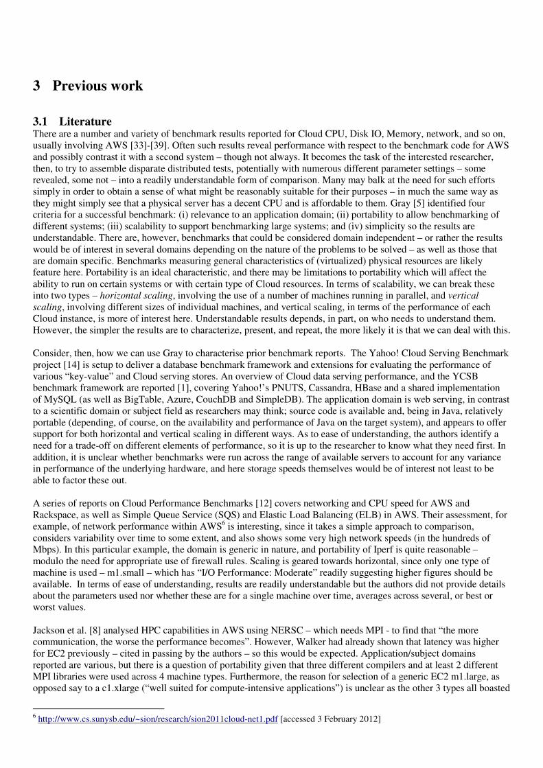
3.2.1 CloudHarmony CloudHarmony [30] has been monitoring the availability of Cloud services (38 in total) since late 2009. Providers monitored range from those offering IaaS such as GoGrid, Rackspace and Amazon Web Services, and PaaS services such as Microsoft Azure and Google App Engine. After consuming an initial offering of 5 tokens in exploring benchmarks, use of the site relies on the purchase of additional tokens priced in various multiples (50, 150, 350 and 850 credits for $30, $85, $180 and $395 respectively). With the right amount of tokens, benchmark reports can be generated for, one benchmark at a time, the regions of the various Cloud providers. The user must decide upon one benchmark to look at, and wait a short time whilst the system populates the set of available Cloud providers (broken into regions – see Figure 1). Results for that benchmark can then be tabulated or displayed on a graph.

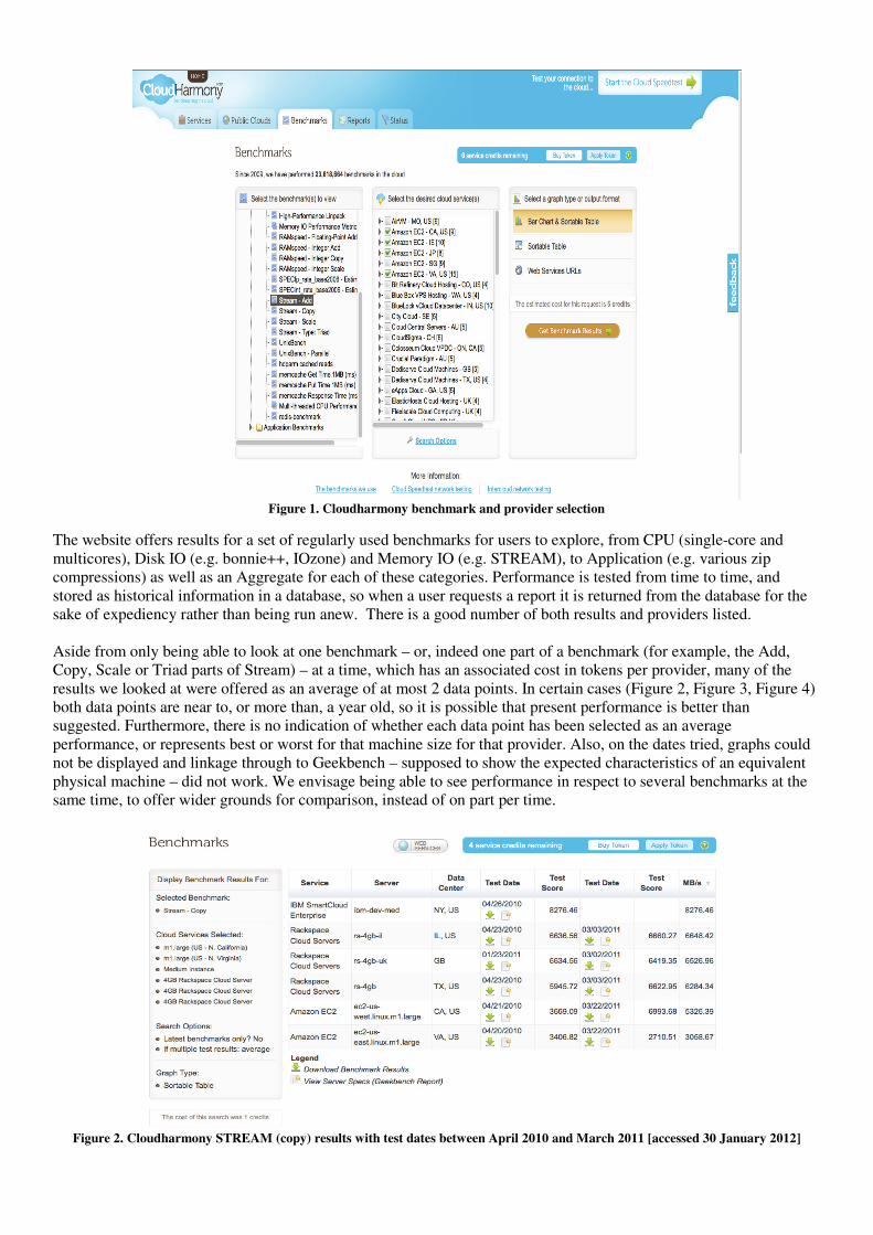
Figure 1. Cloudharmony benchmark and provider selection

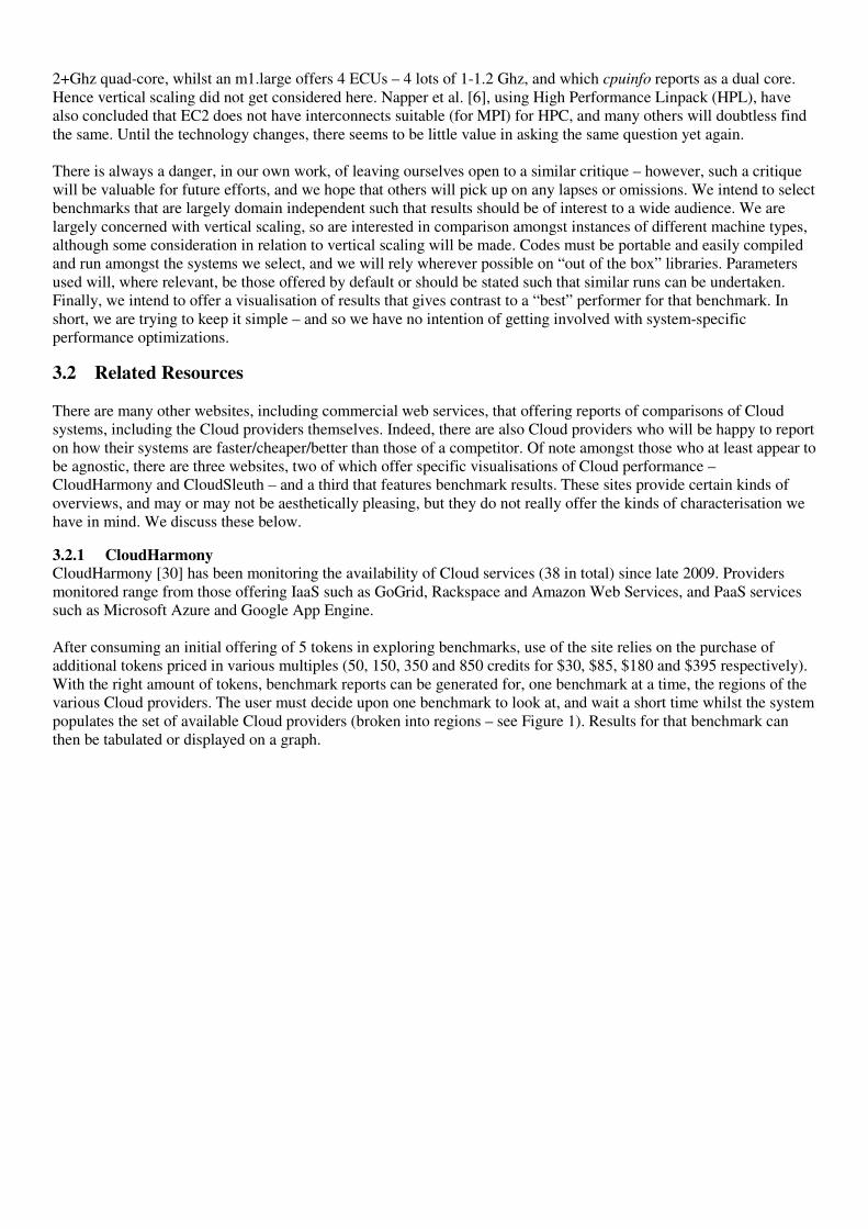
The website offers results for a set of regularly used benchmarks for users to explore, from CPU (single-core and multicores), Disk IO (e.g. bonnie++, IOzone) and Memory IO (e.g. STREAM), to Application (e.g. various zip compressions) as well as an Aggregate for each of these categories. Performance is tested from time to time, and stored as historical information in a database, so when a user requests a report it is returned from the database for the sake of expediency rather than being run anew. There is a good number of both results and providers listed. Aside from only being able to look at one benchmark – or, indeed one part of a benchmark (for example, the Add, Copy, Scale or Triad parts of Stream) – at a time, which has an associated cost in tokens per provider, many of the results we looked at were offered as an average of at most 2 data points. In certain cases (Figure 2, Figure 3, Figure 4) both data points are near to, or more than, a year old, so it is possible that present performance is better than suggested. Furthermore, there is no indication of whether each data point has been selected as an average performance, or represents best or worst for that machine size for that provider. Also, on the dates tried, graphs could not be displayed and linkage through to Geekbench – supposed to show the expected characteristics of an equivalent physical machine – did not work. We envisage being able to see performance in respect to several benchmarks at the same time, to offer wider grounds for comparison, instead of on part per time.

Figure 2. Cloudharmony STREAM (copy) results with test dates between April 2010 and March 2011 [accessed 30 January 2012]

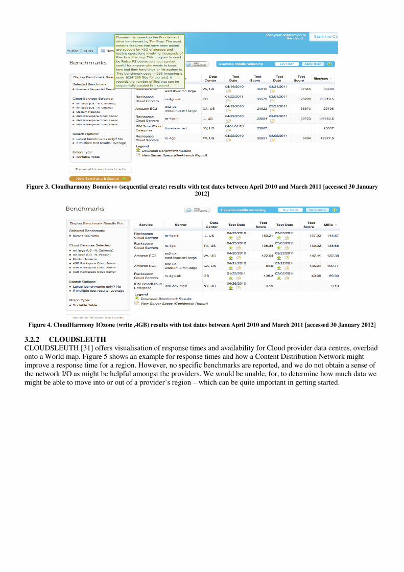
Figure 3. Cloudharmony Bonnie++ (sequential create) results with test dates between April 2010 and March 2011 [accessed 30 January

2012]

Figure 4. CloudHarmony IOzone (write ,4GB) results with test dates between April 2010 and March 2011 [accessed 30 January 2012]

3.2.2 CLOUDSLEUTH CLOUDSLEUTH [31] offers visualisation of response times and availability for Cloud provider data centres, overlaid onto a World map. Figure 5 shows an example for response times and how a Content Distribution Network might improve a response time for a region. However, no specific benchmarks are reported, and we do not obtain a sense of the network I/O as might be helpful amongst the providers. We would be unable, for, to determine how much data we might be able to move into or out of a provider’s region – which can be quite important in getting started.

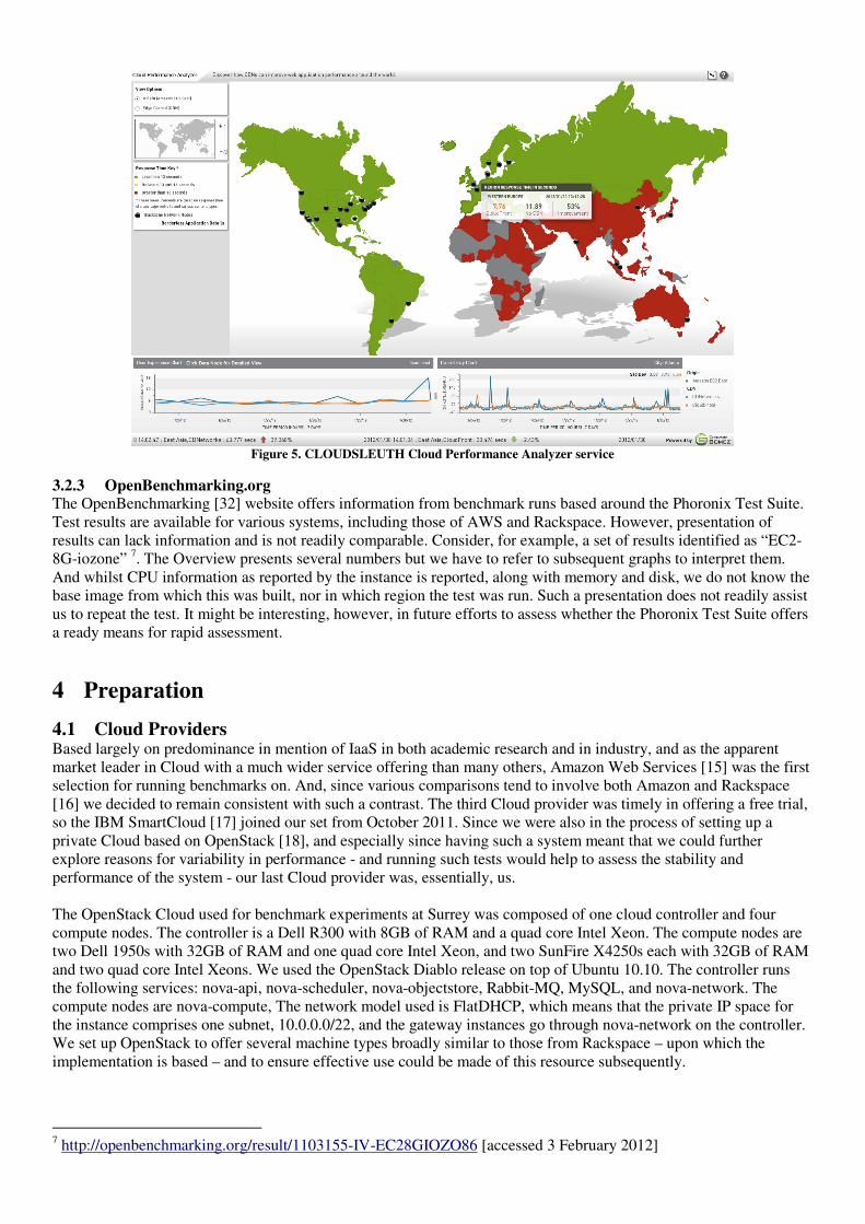
Figure 5. CLOUDSLEUTH Cloud Performance Analyzer service

3.2.3 OpenBenchmarking.org The OpenBenchmarking [32] website offers information from benchmark runs based around the Phoronix Test Suite. Test results are available for various systems, including those of AWS and Rackspace. However, presentation of results can lack information and is not readily comparable. Consider, for example, a set of results identified as “EC2-8G-iozone” 7. The Overview presents several numbers but we have to refer to subsequent graphs to interpret them. And whilst CPU information as reported by the instance is reported, along with memory and disk, we do not know the base image from which this was built, nor in which region the test was run. Such a presentation does not readily assist us to repeat the test. It might be interesting, however, in future efforts to assess whether the Phoronix Test Suite offers a ready means for rapid assessment.

4 Preparation

4.1 Cloud Providers Based largely on predominance in mention of IaaS in both academic research and in industry, and as the apparent market leader in Cloud with a much wider service offering than many others, Amazon Web Services [15] was the first selection for running benchmarks on. And, since various comparisons tend to involve both Amazon and Rackspace [16] we decided to remain consistent with such a contrast. The third Cloud provider was timely in offering a free trial, so the IBM SmartCloud [17] joined our set from October 2011. Since we were also in the process of setting up a private Cloud based on OpenStack [18], and especially since having such a system meant that we could further explore reasons for variability in performance - and running such tests would help to assess the stability and performance of the system - our last Cloud provider was, essentially, us. The OpenStack Cloud used for benchmark experiments at Surrey was composed of one cloud controller and four compute nodes. The controller is a Dell R300 with 8GB of RAM and a quad core Intel Xeon. The compute nodes are two Dell 1950s with 32GB of RAM and one quad core Intel Xeon, and two SunFire X4250s each with 32GB of RAM and two quad core Intel Xeons. We used the OpenStack Diablo release on top of Ubuntu 10.10. The controller runs the following services: nova-api, nova-scheduler, nova-objectstore, Rabbit-MQ, MySQL, and nova-network. The compute nodes are nova-compute, The network model used is FlatDHCP, which means that the private IP space for the instance comprises one subnet, 10.0.0.0/22, and the gateway instances go through nova-network on the controller. We set up OpenStack to offer several machine types broadly similar to those from Rackspace – upon which the implementation is based – and to ensure effective use could be made of this resource subsequently.

7 http://openbenchmarking.org/result/1103155-IV-EC28GIOZO86 [accessed 3 February 2012]

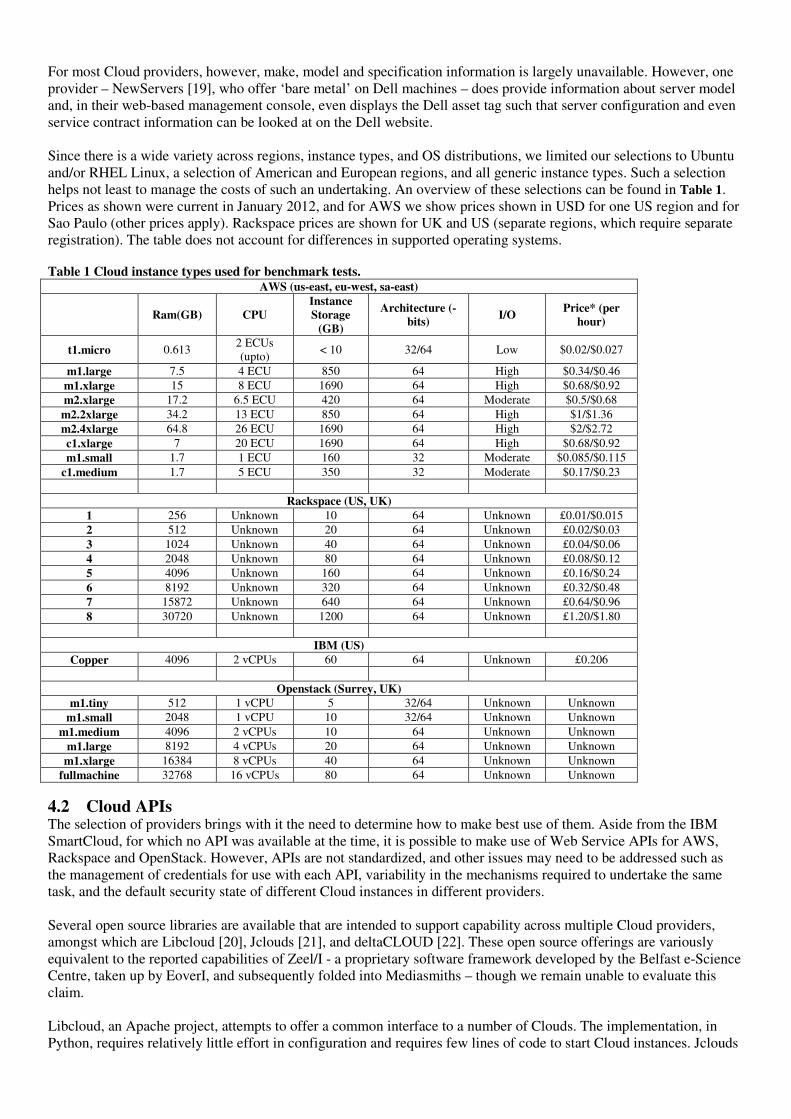
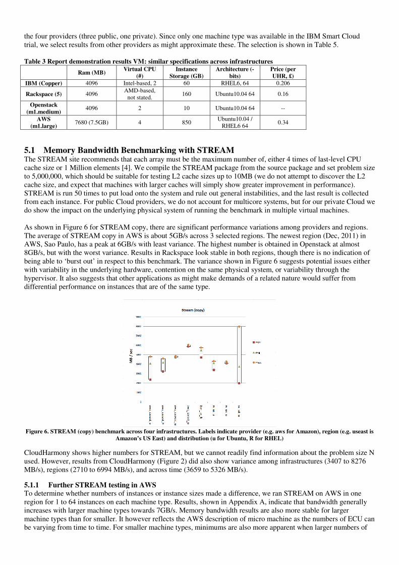
For most Cloud providers, however, make, model and specification information is largely unavailable. However, one provider – NewServers [19], who offer ‘bare metal’ on Dell machines – does provide information about server model and, in their web-based management console, even displays the Dell asset tag such that server configuration and even service contract information can be looked at on the Dell website. Since there is a wide variety across regions, instance types, and OS distributions, we limited our selections to Ubuntu and/or RHEL Linux, a selection of American and European regions, and all generic instance types. Such a selection helps not least to manage the costs of such an undertaking. An overview of these selections can be found in Table 1. Prices as shown were current in January 2012, and for AWS we show prices shown in USD for one US region and for Sao Paulo (other prices apply). Rackspace prices are shown for UK and US (separate regions, which require separate registration). The table does not account for differences in supported operating systems.

Table 1 Cloud instance types used for benchmark tests. AWS (us-east, eu-west, sa-east)

Ram(GB) CPU

Instance

Storage

(GB)

Architecture (-

bits) I/O

Price* (per

hour)

t1.micro 0.613 2 ECUs (upto)

< 10 32/64 Low $0.02/$0.027

m1.large 7.5 4 ECU 850 64 High $0.34/$0.46

m1.xlarge 15 8 ECU 1690 64 High $0.68/$0.92

m2.xlarge 17.2 6.5 ECU 420 64 Moderate $0.5/$0.68

m2.2xlarge 34.2 13 ECU 850 64 High $1/$1.36

m2.4xlarge 64.8 26 ECU 1690 64 High $2/$2.72

c1.xlarge 7 20 ECU 1690 64 High $0.68/$0.92

m1.small 1.7 1 ECU 160 32 Moderate $0.085/$0.115

c1.medium 1.7 5 ECU 350 32 Moderate $0.17/$0.23

Rackspace (US, UK)

1 256 Unknown 10 64 Unknown £0.01/$0.015

2 512 Unknown 20 64 Unknown £0.02/$0.03

3 1024 Unknown 40 64 Unknown £0.04/$0.06

4 2048 Unknown 80 64 Unknown £0.08/$0.12

5 4096 Unknown 160 64 Unknown £0.16/$0.24

6 8192 Unknown 320 64 Unknown £0.32/$0.48

7 15872 Unknown 640 64 Unknown £0.64/$0.96

8 30720 Unknown 1200 64 Unknown £1.20/$1.80

IBM (US)

Copper 4096 2 vCPUs 60 64 Unknown £0.206

Openstack (Surrey, UK)

m1.tiny 512 1 vCPU 5 32/64 Unknown Unknown

m1.small 2048 1 vCPU 10 32/64 Unknown Unknown

m1.medium 4096 2 vCPUs 10 64 Unknown Unknown

m1.large 8192 4 vCPUs 20 64 Unknown Unknown

m1.xlarge 16384 8 vCPUs 40 64 Unknown Unknown

fullmachine 32768 16 vCPUs 80 64 Unknown Unknown

4.2 Cloud APIs The selection of providers brings with it the need to determine how to make best use of them. Aside from the IBM SmartCloud, for which no API was available at the time, it is possible to make use of Web Service APIs for AWS, Rackspace and OpenStack. However, APIs are not standardized, and other issues may need to be addressed such as the management of credentials for use with each API, variability in the mechanisms required to undertake the same task, and the default security state of different Cloud instances in different providers. Several open source libraries are available that are intended to support capability across multiple Cloud providers, amongst which are Libcloud [20], Jclouds [21], and deltaCLOUD [22]. These open source offerings are variously equivalent to the reported capabilities of Zeel/I - a proprietary software framework developed by the Belfast e-Science Centre, taken up by EoverI, and subsequently folded into Mediasmiths – though we remain unable to evaluate this claim. Libcloud, an Apache project, attempts to offer a common interface to a number of Clouds. The implementation, in Python, requires relatively little effort in configuration and requires few lines of code to start Cloud instances. Jclouds

claims to support some 30 Cloud infrastructures’ APIs for Java and Clojure developers but requires substantially more effort to setup and run than libcloud. deltaCLOUD, developed by RedHat and now an Apache project, offers a common RESTful API to a number of Cloud providers, but does not seem to be quite as popular as either of the previous two. Although such libraries claim to support major providers, all had various shortcomings – probably due to the relative immaturity of the libraries which meant that beyond relatively stock tasks – some of which, such as starting up instances – became more awkward to manage, we were largely adapting to Cloud provider-specific differences; it became increasingly difficult to retain compatibility with these libraries. In addition, changes to provider APIs meant we ended up working more and more closely to the provider APIs themselves. In short, working with each API directly became an easier proposition.

4.3 Benchmark selection Cloud Computing benchmarks need to be able to account for various parts of the Cloud “machine” – typically, in IaaS, an instance of a virtual machine – since different applications will depend differently on throughput into and out of the machine (network), and in their reliance on factors of processor speed, memory throughput and storage (disk) both for raw data and as use for swap. Large memory systems with fast storage are likely to be preferred where, for example, large databases are relevant, and there will be a cost to putting such data onto such a system in the first place. Elsewhere, data volumes may be substantially less and CPU performance may be of much greater interest, but can be limited by factors other than its clock speed. Traditional benchmarking involves the benchmark application being ready to run, and information captured about the system only from the benchmark itself. Results of many such benchmarks are offered in isolation – e.g. LINPACK alone for Top500 supercomputers. Whilst this may answer a question in relation to performance of applications with similar requirements to LINPACK, determination for an arbitrary application with different demands on network/CPU/memory/disk requires rather more effort. For our purposes, we want to understand performance in terms of what you can get in a Cloud instance and require a set of benchmarks that tests different aspects of such an instance. Further, we also want to understand an underlying cost (in time and/or money) as necessary to achieve that performance. Put another way, if two Cloud instances achieved equal performance in a benchmark, but one took equally as long to be provisioned as it did to run the benchmark, what might we say about the value-for-money question? Raw performance is just one part of this. Additionally, if performance is variable for Cloud instances of the same type from the same provider, would we want to report only “best” performance? We can also enquire as to whether performance varies over time – either for new instances of the same type, or in relation to continuous use of the same instances over a period. There may be other dimensions to this that would offer valuable future work. The selected benchmarks are intended to treat (i) Memory IO; (ii) CPU; (iii) Disk IO; (iv) Application; (v) Network. This offers a relationship both to existing literature and reports on Cloud performance, and also keys in to the major categories presented by CloudHarmony. There are numerous alternatives available, and reasons for and against selection of just about any individual benchmark. We are largely interested in broad characterisation – and, ideally, in the ready-repeatability of the application of such benchmarks to other Cloud systems.

4.3.1 Memory IO The rate at which the processor can interact with memory offers one potential system bottleneck. Server specifications often cite a maximum potential bandwidth, for example the cited maximum for one of our OpenStack Sun Fire x4250s is 21GB/s, (with a 6MB L2 cache). Cloud providers do not cite figures for memory bandwidth, even though the ability to make effective use of the CPU for certain types of workload is going to be governed to some extent by whether the virtualisation system (hypervisor), base operating system or hardware itself can sufficiently separate operations to deal with any contention for the underlying physical resources.

4.3.1.1 STREAM

STREAM [23] is regarded as a standard synthetic benchmark for the measurement of memory bandwidth. From the perspective of applications, the benchmark attempts to determine a sustainable “realistic” memory bandwidth, which is unlikely to be the same as the theoretical peak, using four vector-based operations: COPY a=b, SCALE a=q*b, SUM a=b+c and TRIAD a=b+q*c.

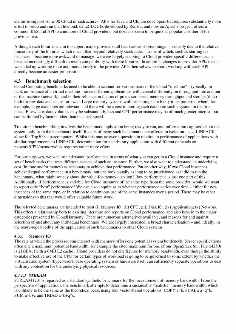
4.3.2 CPU There are various measures to determine CPU capabilities. We might get a sense of the speed (GHz) of the processor from the provider – which for Amazon is stated as a multiple of the “CPU capacity of a 1.0-1.2 GHz 2007 Opteron or 2007 Xeon processor” although this gives us no additional related information regarding the hardware. On the other hand, we might find such information entirely elusive, and only be able to find out, for example for Rackspace, that “Comparing Cloud Servers to standard EC2 instances our vCPU assignments are comparable” or that the number of vCPUs increases with larger memory sizes, or see a number of vCPUs as offered to Windows-based systems. Rackspace also suggest an advantage in being able to ‘burst’ into spare CPU capacity on a physical machine – but since we cannot readily discover information about the underlying system we will not know whether we might be so fortunate at any given time.

Source: http://www.rackspace.com/cloud/blog/2010/07/22/cloud-servers-for-windows-beta-update/ When we start a Cloud instance, we might enquire in the instance as regards reported processor information (for example in /proc/cpuinfo). However there is a possibility that such information has been modified.

4.3.2.1 LINPACK

LINPACK [26] measures the floating point operations per second (flop/s) for a set of linear equations. It is the benchmark of choice for the Top500 supercomputers list, where it is used to identify a maximal performance for a maximal problem size. It would be expected that systems would be optimized specifically to such a benchmark, however we will be interested in the unoptimized performance of Cloud instances since this is what the typical user would get.

4.3.3 Disk I/O Any significantly data-intensive application is going to be heavily dependent on various factors of the underlying data storage system. A Cloud provider will offer a certain amount of storage with a Cloud instance by default, and often it is possible to add further storage volumes. Typically, we might address three different kinds of Cloud storage: 1. instance storage, most likely the disk physically installed in the underlying server; 2. attached storage, potentially mounted from a storage array of some kind, for example using ATA over Ethernet (AoE) or iSCSI; 3. “object” storage. Instance storage might or might not be offered with some kind of redundancy to allow for recovery in the event of disk failure, but all contents are likely to be wiped once the resource is no longer in use. Attached storage may be detachable, and offers at least three other opportunities (i) to retain images whilst not in use just as stored data, rather than keeping them live on systems – which can be less expensive; (ii) faster startup times of instances based on images stored in this way; (iii) faster snapshots than for instance storage. Attached storage may also operate to automatically retain a redundant copy. Object storage (for example S3 from Amazon, and Cloud Files from Rackspace) tends to be geared towards direct internet accessibility of files that are intended to have high levels of redundancy and which may be effectively coupled with Content Distribution Networks. Consequently, Object storage is unlikely to be suited to heavy I/O needs and so our disk I/O considerations will be limited to instance storage and attached storage. However, while the Cloud providers will say how much storage, they do not typically state how fast. We selected 2 benchmarks for storage to ascertain whether more or fewer metrics would be more readily understandable.

4.3.3.1 Bonnie++

Bonnie++ [24] is a further development of Bonnie, a well-known Disk IO performance benchmark suite that uses a series of simple tests to derive performance relating to:

i. Data read and write speeds; ii. Maximum number of seeks per second;

iii. Maximum number of file metadata operations per second (includes file creation, deletion or gathering of file information)

4.3.3.2 IOzone

IOzone [25] offers 13 performance metrics and reports values for read, write, re-read, rewrite, random read, random write, backward read, record re-write, stride read, Fread, Fwrite, Fre-read, and Fre-write.

4.3.4 Application (Compression) A particular application may create demand on various different parts of the system. The time taken to compress a given (large) file is going to depend on the read and write operations and throughput to CPU. With sufficient information obtained from other benchmarks, it may become possible to estimate the effects on an application of a given variability – for example, a 5% variation in disk speed, or substantial variation in available memory bandwidth

4.3.4.1 Bzip2

bzip2 [29] is an application for compressing files based on the Burrows-Wheeler Algorithm. It is a CPU bound task with a small amount of I/O and as such is also useful for benchmarking CPUs. A slightly modified version is included in SPEC CPU2006 benchmark suite [29] and the standard version, as found on any Linux system, is used as part of the phoronix test suite. There is also a multi threaded version, pbzip2, which can be used to benchmark multi-core systems.

4.3.5 Network CloudHarmony does not offer us information regarding network speeds. CloudSleuth offers response times, but not from where we might want to migrate data to and from, and also does not indicate bandwidth. If we were thinking to do “Big Data” in the Cloud, such data is very useful to us. Our interest in upload and download speeds will depend on how much needs to move where. So, for example, if we were undertaking analysis of a Wikipedia dump, we’d likely want a fast download to the provider and download of results from the provider to us may be rather less important (costs of an instance will be accrued during the data transfer, as well as the costs of any network I/O if charged by the provider). It is worth noting that some providers offer a service by which physical disks can be shipped to them for copying. Amazon offers just such a service, and also hosts a number of data volumes (EBS) that can be instanced and attached to instances8. Depending on the nature of work being done, there is potential interest also in at least three other aspects to network performance: (i) general connectivity within the provider (typically within a region); (ii) specific connectivity in relation to any co-located instances as might be relevant to HPC-type activities; (iii) connectivity amongst providers and regions such that data might be migrated to benefit from cost differences. The latter also offers a good indication general network bandwidth (and proximity) for these providers.

4.3.5.1 Iperf

Iperf [27] was developed by NLANR (National Laboratory for Applied Network Research)/DAST (Distributed Applications Support Team) to measure and test network bandwidth, latency, and transmission loss. It is often used as a means to determine overall quality of a network link. Use of Iperf should be suited to tests between Cloud providers and to/from host institutions. However it will not offer measurements for connections to data hosted elsewhere.

4.3.5.2 MPPTEST

MPPTEST [28], from Argonne National Labs (ANL), measures performance of network connections used for message passing (MPI). With general network connectivity assessed using Iperf, MPPTEST would offer suitability in respect to HPC-type activities where Cloud providers are specifically targeting such kinds of workloads.

4.3.5.3 Simple speed tests

For general download operations, such as that of a Wikipedia dump, applications such as scp, curl, and wget can be used to obtain a simple indication of speed in relation to elapsed time. Such a download, in different Cloud provider regions, can also indicate whether such data might be being offered via a CDN.

4.4 The Cloud instance sequence A Cloud resource generally, and a Cloud machine instance in particular has several stages, all of which can take time and so can attract cost. We will set aside the uncosted element of the user determining what they want to use, for obvious reasons of comparability. If we now take AWS as an example provider, the user will first issue a request to run an instance of a specific type. When the provider receives the request, this will start the boot process for a virtual machine, and charging typically begins at receipt of the request. After the virtual machine has booted, the user will

8 See: http://aws.amazon.com/datasets/ for a list of such datasets [accessed 3 February 2012].

need to setup the system to the point they require, including installing security updates, application dependencies, and the application (e.g. benchmark) itself. Finally, the application can be run. At the end, the resource is released. The sequence from receipt of request to final release, which includes the time for shutdown of the instance, incurs costs. It is interesting to note that we have seen variation in boot times for AWS depending on where the request is made from. If issued outside AWS, the acknowledgement is returned within about 3 seconds. Otherwise, it can take 90 seconds or so. This has an impact to total run time and potentially also to cost depending on how instances are priced. We will take external times for all runs. Costs are applicable for most providers once a request has been issued, which means that boot time has to be paid for even though the instance is not ready to use – this might be thought of as akin to paying for a telephone call from the moment the last digit is pressed; indeed, we can extend this analogy further as you may also end up paying even if the call fails for any reason and, indeed, may pay the minimum unit cost for this (more about this later in this report). Subsequently, applying patches will be a factor of the number to be applied and the speed of connection to relevant repositories, and so will also have an associated cost.

5 Cloud Benchmark results – a sample Our selected benchmarks are, typically, run using Linux distributions in all 4 infrastructures - if it is possible to do so and it makes sense to do so – with the obvious exception of network benchmarks. We use Cloud provider images of Ubuntu 10.04 where available, but since the trial of IBM Smart Cloud offered only RHEL6 we also use a RHEL6 image in EC2 to be able to offer comparisons. The AWS instances are all EBS backed, which offers faster boot times than instance backed. Use of different operating systems leads to variation in how updates are made, but since we consider this “out of the box” the Ubuntu updates occur through apt-get whilst for RHEL we used yum. In addition, we have to account for variation in access mechanisms to the instances: Amazon EC2 and Openstack API provide SSH key based authentication by default, but the SSH service needs to be reconfigured for IBM and Rackspace. After this small modification to our setup phase, we snapshot running instances which gives us a slightly modified start point but otherwise retains the sequence described above. Table 2 Cloud image ids used for benchmark tests. aws-us-east aws-us-west

oregon

aws-sa-east Rackspace UK Rackspace US IBM

Ubuntu_64(10.10) ami-2ec83147 ami-c4fe73f4 ami-ec3ae5f1 15099429 10318018 n/a

Ubuntu_32(10.10) ami-2cc83145 ami-defe73ee ami-6235ea7f n/a n/a n/a

RHEL_64(6.1) ami-31d41658 n/a n/a n/a n/a available RHEL 6.1

RHEL_32(6.1) ami-3ddb1954 n/a n/a n/a n/a n/a

A benchmark can be set up and run immediately after a new (modified) instance is provisioned. We account for the booting time of an instance, and the remaining time taken to setup – applying available patches – the instance appropriately for each benchmark to be run. Also as part of setup, each benchmark is downloaded, along with any dependencies and, if necessary, compiled – again, costs will be associated to connection speed to the benchmark source, and time taken for the compiler – and run. Once the benchmark is complete, results are sent to a server and the instance can be released. The cost of running a benchmark is, then, some factor of the cost of the benchmark itself and the startup and shutdown costs relating to enabling it to run. This will be the case for any application unless snapshots of runnable systems are used – and these will have an associated cost for storage, so there will be a trade-off between costs of setup and costs of storage for such instances, with the number of instances needed being a multiplier. So, performance of a particular benchmark for a provider could be considered with respect specifically to performance information from the benchmark, or could alternatively be considered with respect to the overall time and cost related to achieving that performance – better benchmark performance may cost more and take longer to achieve, so we might think to distinguish between “system” and “instance” and spread performance across cost and time. All but one of the benchmarks was run across all selected Cloud providers within selected regions on all available machine types. 10 instances of each type were run to obtain information about variability. Due to the sheer number of results obtained, in this section we limit our focus primarily to one set of (relatively) comparable machine types across

the four providers (three public, one private). Since only one machine type was available in the IBM Smart Cloud trial, we select results from other providers as might approximate these. The selection is shown in Table 5. Table 3 Report demonstration results VM: similar specifications across infrastructures

Ram (MB) Virtual CPU

(#)

Instance

Storage (GB)

Architecture (-

bits)

Price (per

UHR, £)

IBM (Copper) 4096 Intel-based, 2 60 RHEL6, 64 0.206

Rackspace (5) 4096 AMD-based,

not stated. 160 Ubuntu10.04 64 0.16

Openstack

(m1.medium) 4096 2 10 Ubuntu10.04 64 --

AWS

(m1.large) 7680 (7.5GB) 4 850

Ubuntu10.04 / RHEL6 64

0.34

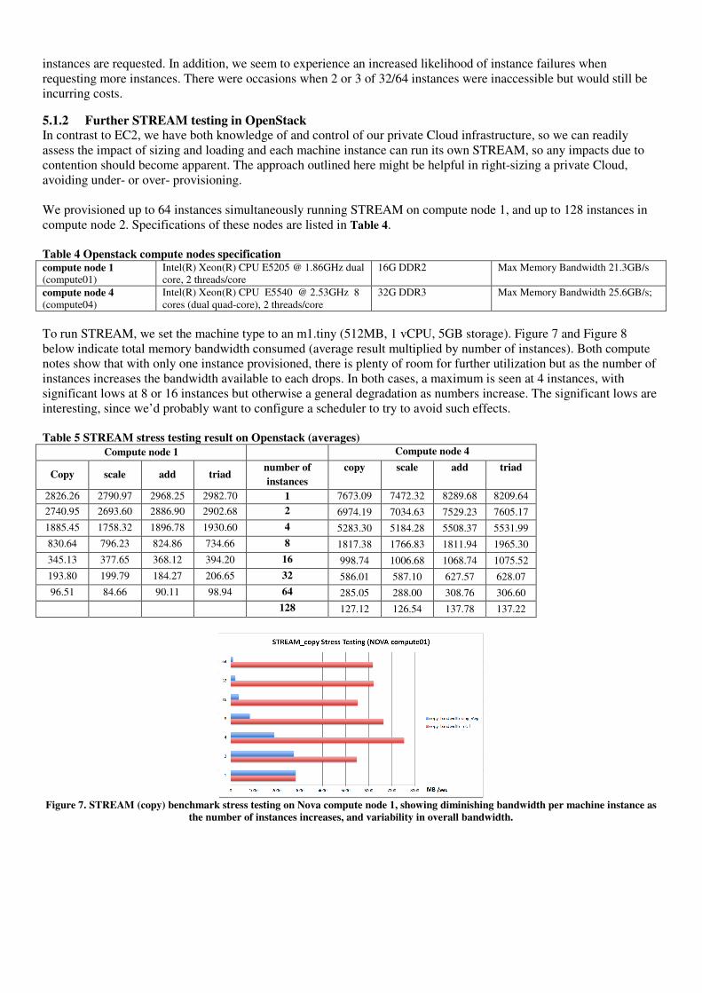
5.1 Memory Bandwidth Benchmarking with STREAM The STREAM site recommends that each array must be the maximum number of, either 4 times of last-level CPU cache size or 1 Million elements [4]. We compile the STREAM package from the source package and set problem size to 5,000,000, which should be suitable for testing L2 cache sizes up to 10MB (we do not attempt to discover the L2 cache size, and expect that machines with larger caches will simply show greater improvement in performance). STREAM is run 50 times to put load onto the system and rule out general instabilities, and the last result is collected from each instance. For public Cloud providers, we do not account for multicore systems, but for our private Cloud we do show the impact on the underlying physical system of running the benchmark in multiple virtual machines. As shown in Figure 6 for STREAM copy, there are significant performance variations among providers and regions. The average of STREAM copy in AWS is about 5GB/s across 3 selected regions. The newest region (Dec, 2011) in AWS, Sao Paulo, has a peak at 6GB/s with least variance. The highest number is obtained in Openstack at almost 8GB/s, but with the worst variance. Results in Rackspace look stable in both regions, though there is no indication of being able to ‘burst out’ in respect to this benchmark. The variance shown in Figure 6 suggests potential issues either with variability in the underlying hardware, contention on the same physical system, or variability through the hypervisor. It also suggests that other applications as might make demands of a related nature would suffer from differential performance on instances that are of the same type.

Figure 6. STREAM (copy) benchmark across four infrastructures. Labels indicate provider (e.g. aws for Amazon), region (e.g. useast is

Amazon’s US East) and distribution (u for Ubuntu, R for RHEL)

CloudHarmony shows higher numbers for STREAM, but we cannot readily find information about the problem size N used. However, results from CloudHarmony (Figure 2) did also show variance among infrastructures (3407 to 8276 MB/s), regions (2710 to 6994 MB/s), and across time (3659 to 5326 MB/s).

5.1.1 Further STREAM testing in AWS To determine whether numbers of instances or instance sizes made a difference, we ran STREAM on AWS in one region for 1 to 64 instances on each machine type. Results, shown in Appendix A, indicate that bandwidth generally increases with larger machine types towards 7GB/s. Memory bandwidth results are also more stable for larger machine types than for smaller. It however reflects the AWS description of micro machine as the numbers of ECU can be varying from time to time. For smaller machine types, minimums are also more apparent when larger numbers of

instances are requested. In addition, we seem to experience an increased likelihood of instance failures when requesting more instances. There were occasions when 2 or 3 of 32/64 instances were inaccessible but would still be incurring costs.

5.1.2 Further STREAM testing in OpenStack In contrast to EC2, we have both knowledge of and control of our private Cloud infrastructure, so we can readily assess the impact of sizing and loading and each machine instance can run its own STREAM, so any impacts due to contention should become apparent. The approach outlined here might be helpful in right-sizing a private Cloud, avoiding under- or over- provisioning. We provisioned up to 64 instances simultaneously running STREAM on compute node 1, and up to 128 instances in compute node 2. Specifications of these nodes are listed in Table 4. Table 4 Openstack compute nodes specification compute node 1 (compute01)

Intel(R) Xeon(R) CPU E5205 @ 1.86GHz dual core, 2 threads/core

16G DDR2 Max Memory Bandwidth 21.3GB/s

compute node 4 (compute04)

Intel(R) Xeon(R) CPU E5540 @ 2.53GHz 8 cores (dual quad-core), 2 threads/core

32G DDR3 Max Memory Bandwidth 25.6GB/s;

To run STREAM, we set the machine type to an m1.tiny (512MB, 1 vCPU, 5GB storage). Figure 7 and Figure 8 below indicate total memory bandwidth consumed (average result multiplied by number of instances). Both compute notes show that with only one instance provisioned, there is plenty of room for further utilization but as the number of instances increases the bandwidth available to each drops. In both cases, a maximum is seen at 4 instances, with significant lows at 8 or 16 instances but otherwise a general degradation as numbers increase. The significant lows are interesting, since we’d probably want to configure a scheduler to try to avoid such effects. Table 5 STREAM stress testing result on Openstack (averages)

Compute node 1 Compute node 4

Copy scale add triad number of

instances

copy scale add triad

2826.26 2790.97 2968.25 2982.70 1 7673.09 7472.32 8289.68 8209.64

2740.95 2693.60 2886.90 2902.68 2 6974.19 7034.63 7529.23 7605.17

1885.45 1758.32 1896.78 1930.60 4 5283.30 5184.28 5508.37 5531.99

830.64 796.23 824.86 734.66 8 1817.38 1766.83 1811.94 1965.30

345.13 377.65 368.12 394.20 16 998.74 1006.68 1068.74 1075.52

193.80 199.79 184.27 206.65 32 586.01 587.10 627.57 628.07

96.51 84.66 90.11 98.94 64 285.05 288.00 308.76 306.60

128 127.12 126.54 137.78 137.22

Figure 7. STREAM (copy) benchmark stress testing on Nova compute node 1, showing diminishing bandwidth per machine instance as

the number of instances increases, and variability in overall bandwidth.

Figure 8. STREAM (copy) benchmark stress testing on Nova compute04, showing diminishing bandwidth per machine instance as the

number of instances increases, and variability in overall bandwidth

5.2 Disk I/O Performance Benchmarking with bonnie++ and IOZone.

5.2.1 Bonnie++ We use the standard package library of Bonnie++ from the Ubuntu multiverse repository with no special tuning. However, disk space for testing should be twice the size of RAM. All the machine types used could offer this, so /tmp was readily usable for tests.

Figure 9. Bonnie++ (sequential create) benchmark across four infrastructures

Figure 9 shows results for Bonnie++ for sequential creation of files per second (we could not get results for this from Rackspace UK for some reason). Our Openstack instances again show high performance (peak is almost 30k files/second) but with high variance. The distance of best-performed boxes among EC2 regions is about 10000 apart, but the averages are much closer. Results shown on the CloudHarmony website are much higher, but this could be because they are using a file size of 4GB, whereas our test is using the default setting (double size of the memory) in EC2 for the more accurate results as suggest by Bonnie++ literature.

5.2.2 IOzone IOzone is also available from the Ubuntu multiverse repository. We use automatic mode, file size of 2GB, 1024 records, and output for Excel. The results shown Figure 10 show wide variance but better performance for Rackspace (and worst for our Openstack Cloud with average less than 60 MB/Sec).

Figure 10. IOzone (write, file size: 2G, records size: 1024) benchmark across four infrastructures

5.3 CPU Performance Benchmarking

5.3.1 LINPACK We obtained LINPACK from the Intel website, and since it is available pre-compiled, we can run it using the defaults given, which test the problem size and leading dimensions from 1000 to 45000. Rackspace is based on AMD, and although it is possible to configure LINPACK for AMD, we decided the efforts would be best put elsewhere. Results for Rackspace are therefore absent from Figure 11, and we dropped the use of LINPACK for the AWS US East region because we assumed by this stage that figures would be largely comparable to the other two regions.

Figure 11. LINPACK (25000 tests) benchmark across tested infrastructures

AWS instances produce largely similar results, without significant variance. Our OpenStack Cloud again suffers in performance – perhaps a reflection on the age of the servers.

5.3.2 Application (Compression) Performance with Bzip2 Since variance was clearly an issue, we would already anticipate similar variance to occur in applications. We therefore changed strategy to see whether performance variation was significant over longer time periods. We launched three AWS m1.small instances from ami-6936fb00 in the US East region. For this test, we created a tarball out of the root file system and used bzip2 to compress this file. After 3 minutes, the compressed file was deleted and the compression operation repeated. We ran these instances for close to 2 weeks, collecting timing information about the duration of the compression operation, and collected 1500 data points from each instance (Figure 9).

Figure 12 Bzip2 compression test in EC2

Across all three instances, the fastest time recorded was 382s whilst the slowest was 896s. Results are summaries in Table 6 below. Table 6 Bzip2 compression test results

A B C

min 438.25 502.51 381.58

avg 623.467 570.5648667 538.5978133

max 895.83 762.01 673.86

SD 55.74547111 51.78058942 47.86779689

Despite all three instances being of the same type, machineA is consistently slower than both machineB and machineC. We also see that machineA has greater variation in performance over the first 50 data points and the standard deviation here is 82.96. Interestingly, performance for all three improves by over 100 seconds over time – however, there would be a cost associated with waiting for performance improvement!

5.4 Network Benchmarking

5.4.1 Iperf With Iperf, we were interested in identifying preferred options for dealing with large volumes of data. Previous benchmarks can account for various characteristics of the machine instances running at Cloud providers, but with Iperf we are determining the potential for pushing data to or pulling it from the Cloud providers. As our IBM SmartCloud trial had ended, we decided that we might try to offer further perspective on the data question by adding the National Grid Services (NGS) to our considerations. Furthermore, since a researcher inside an institution might have a choice between using a desktop system and a private Cloud (or other server), we wanted to assess the capabilities of both. For our public Cloud providers, we used two regions of AWS (us-east-1 and eu-west-1) and two of Rackspace (US and UK). Specifications of machines used are show in Table 9. Table 7 Iperf benchmark test environment comparison

Openstack

(m1.small, Ubuntu

10.04)

Surrey local workstation

(Ubuntu 10.04)

AWS EC2 (m1.small,

Ubuntu 10.04)

Rackspace (2048M,

Ubuntu 10.04)

NGS (ngs.rl.ac.uk,

RHEL 4)

2GB memory 64-bit OS

Intel Core 2 Duo 3.16GHz 2GB memory

64-bit OS

1.7 GB memory 1 virtual core with 1 EC2

Compute Unit 32-bit OS

2GB memory 64-bit OS

AMD Dual-Core Opteron 880s (8 cores), 2.4GHz

3GB memory 64-bit OS

The benchmark is tested in TCP mode across infrastructures in a simple client-server manner, with transmit size of 50MB (“-n”), single directional test and default TCP window size. Firewall configurations at Surrey and NGS necessitated adjustments to how the experiments might have been performed. At Surrey, iperf could only act as a client. NGS could readily act as client, but could only act as server in the GLOBUS_TCP_PORT_RANGE. Restrictions are illustrated in Figure 13.

Figure 13. iperf benchmark testing work flow

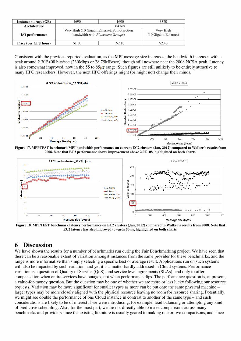
Tests were conducted first with 10 clients contacting 1 server, then with 1 client contacting 10 servers. Turns are evaluated at different times of the day to account for variable network loads in different regions. Figure 14 shows the bandwidth performance between the 2 regions of each of the 2 public Cloud providers, with interesting peak results when AWS is on the client side in the same region, with peaks of some 250MB/s but a clear lack of reciprocity. Figure 15 shows connections between NGS and the public Clouds, with a single peak around 100MB/s with Rackspace UK – again with Rackspace acting on the server side. This (isolated) set of tests does suggest that migrating data across Clouds would be quicker than migrating to and from Clouds from NGS. Figure 16 shows yet more relatively disappointing results from Surrey’s OpenStack. Performance problems were also experienced with desktop workstations and other servers on which we tried iperf also. However, general download speed from the web is reasonable (for example an average 2.98MB/s from Ubuntu.com). Further understanding of the local network configuration is likely necessary to uncover the reasons for this.

Figure 14. Bandwidth results between AWS and Rackspace of US and EU region using iperf benchmark

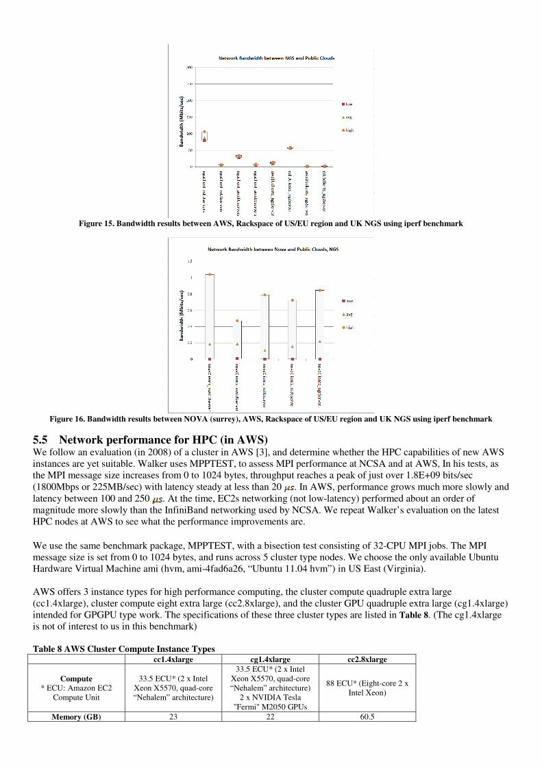
Figure 15. Bandwidth results between AWS, Rackspace of US/EU region and UK NGS using iperf benchmark

Figure 16. Bandwidth results between NOVA (surrey), AWS, Rackspace of US/EU region and UK NGS using iperf benchmark

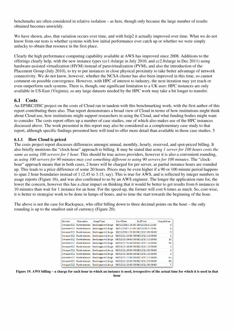
5.5 Network performance for HPC (in AWS) We follow an evaluation (in 2008) of a cluster in AWS [3], and determine whether the HPC capabilities of new AWS instances are yet suitable. Walker uses MPPTEST, to assess MPI performance at NCSA and at AWS, In his tests, as the MPI message size increases from 0 to 1024 bytes, throughput reaches a peak of just over 1.8E+09 bits/sec (1800Mbps or 225MB/sec) with latency steady at less than 20 . In AWS, performance grows much more slowly and latency between 100 and 250 . At the time, EC2s networking (not low-latency) performed about an order of magnitude more slowly than the InfiniBand networking used by NCSA. We repeat Walker’s evaluation on the latest HPC nodes at AWS to see what the performance improvements are.

We use the same benchmark package, MPPTEST, with a bisection test consisting of 32-CPU MPI jobs. The MPI message size is set from 0 to 1024 bytes, and runs across 5 cluster type nodes. We choose the only available Ubuntu Hardware Virtual Machine ami (hvm, ami-4fad6a26, “Ubuntu 11.04 hvm”) in US East (Virginia). AWS offers 3 instance types for high performance computing, the cluster compute quadruple extra large (cc1.4xlarge), cluster compute eight extra large (cc2.8xlarge), and the cluster GPU quadruple extra large (cg1.4xlarge) intended for GPGPU type work. The specifications of these three cluster types are listed in Table 8. (The cg1.4xlarge is not of interest to us in this benchmark) Table 8 AWS Cluster Compute Instance Types

cc1.4xlarge cg1.4xlarge cc2.8xlarge

Compute * ECU: Amazon EC2

Compute Unit

33.5 ECU* (2 x Intel Xeon X5570, quad-core “Nehalem” architecture)

33.5 ECU* (2 x Intel Xeon X5570, quad-core “Nehalem” architecture)

2 x NVIDIA Tesla "Fermi" M2050 GPUs

88 ECU* (Eight-core 2 x Intel Xeon)

Memory (GB) 23 22 60.5

Instance storage (GB) 1690 1690 3370

Architecture 64 bits

I/O performance

Very High (10 Gigabit Ethernet. Full-bisection bandwidth with Placement Groups)

Very High (10 Gigabit Ethernet)

Price (per CPU hour) $1.30 $2.10 $2.40

Consistent with the previous reported evaluation, as the MPI message size increases, the bandwidth increases with a peak around 2.30E+08 bits/sec (230Mbps or 28.75MB/sec), though still nowhere near the 2008 NCSA peak. Latency is also somewhat improved, now in the 55 to 85 range. Such figures are still unlikely to be entirely attractive to many HPC researchers. However, the next HPC offerings might (or might not) change their minds.

Figure 17. MPPTEST benchmark MPI bandwidth performance on current EC2 clusters (Jan, 2012) compared to Walker’s results from

2008. Note that EC2 performance shows improvement above 2.0E+08, highlighted on both charts.

Figure 18. MPPTEST benchmark latency performance on EC2 clusters (Jan, 2012) compared to Walker’s results from 2008. Note that

EC2 latency has also improved towards 50 µs, highlighted on both charts.

6 Discussion We have shown the results for a number of benchmarks run during the Fair Benchmarking project. We have seen that there can be a reasonable extent of variation amongst instances from the same provider for these benchmarks, and the range is more informative than simply selecting a specific best or average result. Applications run on such systems will also be impacted by such variation, and yet it is a matter hardly addressed in Cloud systems. Performance variation is a question of Quality of Service (QoS), and service level agreements (SLAs) tend only to offer compensation when entire services have outages, not when performance dips. The performance question is, at present, a value-for-money question. But the question may be one of whether we are more or less lucky following our resource requests. Variation may be more significant for smaller types as more can be put onto the same physical machine –larger types may be more closely aligned with the physical resource leaving no room for resource sharing. Potentially, we might see double the performance of one Cloud instance in contrast to another of the same type – and such considerations are likely to be of interest if we were introducing, for example, load balancing or attempting any kind of predictive scheduling. Also, for the most part, we are not directly able to make comparisons across many benchmarks and providers since the existing literature is usually geared to making one or two comparisons, and since

benchmarks are often considered in relative isolation – as here, though only because the large number of results obtained becomes unwieldy. We have shown, also, that variation occurs over time, and with bzip2 it actually improved over time. What we do not know from our tests is whether systems with low initial performance ever catch up or whether we were simply unlucky to obtain that resource in the first place. Clearly the high performance computing capability available at AWS has improved since 2008. Additions to the offerings clearly help, with the new instance types (cc1.4xlarge in July 2010, and cc2.8xlarge in Dec 2011) using hardware-assisted virtualization (HVM) instead of paravirtualization (PVM), and also the introduction of the Placement Group (July 2010), to try to put instances in close physical proximity to take better advantage of network connectivity. We do not know, however, whether the NCSA cluster has also been improved in this time, so cannot comment on possible convergence. However, with HPC of interest to industry, the next iteration may yet reach or even outperform such systems. There is, though, one significant limitation to a UK user: HPC instances are only available in US-East (Virginia), so any large datasets needed by the HPC work may take a bit longer to transfer.

6.1 Costs An EPSRC/JISC project on the costs of Cloud ran in tandem with this benchmarking work, with the first author of this report contributing there also. That report demonstrates a broad view of Cloud in terms of how institutions might think about Cloud use, how institutions might support researchers in using the Cloud, and what funding bodies might want to consider. The costs report offers up a number of case studies, one of which also makes use of the HPC instances discussed above. The work presented in this report may also be considered as a complementary case study to that report, although specific findings presented here will tend to offer more detail than available in those case studies. 5

6.1.1 How Cloud is priced The costs project report discusses differences amongst annual, monthly, hourly, reserved, and spot-priced billing. It also briefly mentions the “clock-hour” approach to billing. It may be stated that using 1 server for 100 hours costs the

same as using 100 servers for 1 hour. This should be true across providers, however it is also a convenient rounding, as using 100 servers for 90 minutes may cost something different to using 90 servers for 100 minutes. The “clock-hour” approach means that in both cases, 2 hours will be charged for per server, as partial instance hours are rounded up. This leads to a price difference of some 20 hours. Prices may be even higher if a 90 or 100 minute period happens to span 2 hour boundaries instead of 1 (2.45 to 3.15, say). This is true for AWS, and is reflected by integer numbers in usage reports (Figure 16), and was also confirmed to us by an AWS engineer. The longer the application runs for, the lower the concern, however this has a clear impact on thinking that it would be better to get results from 6 instances in 10 minutes than wait for 1 instance for an hour. For the speed-up, the former will cost 6 times as much. So, cost-wise, it is better to strategise work to be done in lumps of hours, and to time the start towards the beginning of the hour. The above is not the case for Rackspace, who offer billing down to three decimal points on the hour – the only rounding is up to the smallest unit of currency (Figure 20).

Figure 19. AWS billing – a charge for each hour in which an instance is used, irrespective of the actual time for which it is used in that

hour

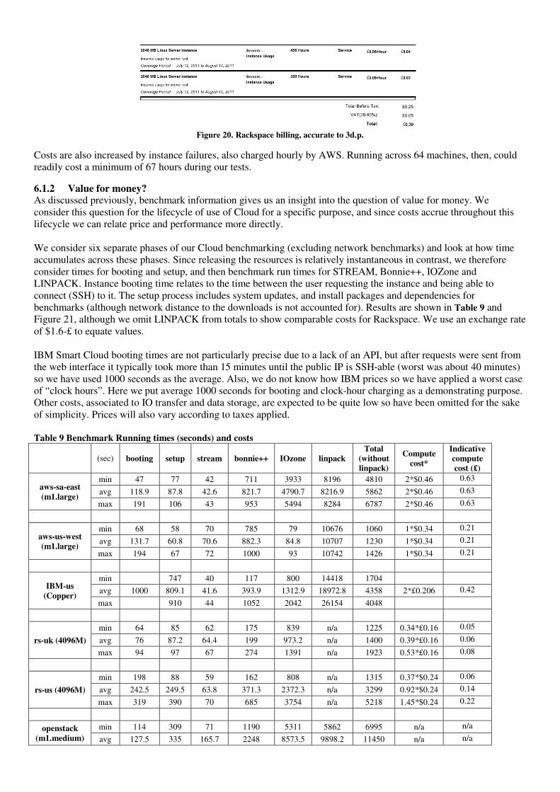
Figure 20. Rackspace billing, accurate to 3d.p.

Costs are also increased by instance failures, also charged hourly by AWS. Running across 64 machines, then, could readily cost a minimum of 67 hours during our tests.

6.1.2 Value for money? As discussed previously, benchmark information gives us an insight into the question of value for money. We consider this question for the lifecycle of use of Cloud for a specific purpose, and since costs accrue throughout this lifecycle we can relate price and performance more directly. We consider six separate phases of our Cloud benchmarking (excluding network benchmarks) and look at how time accumulates across these phases. Since releasing the resources is relatively instantaneous in contrast, we therefore consider times for booting and setup, and then benchmark run times for STREAM, Bonnie++, IOZone and LINPACK. Instance booting time relates to the time between the user requesting the instance and being able to connect (SSH) to it. The setup process includes system updates, and install packages and dependencies for benchmarks (although network distance to the downloads is not accounted for). Results are shown in Table 9 and Figure 21, although we omit LINPACK from totals to show comparable costs for Rackspace. We use an exchange rate of $1.6-£ to equate values. IBM Smart Cloud booting times are not particularly precise due to a lack of an API, but after requests were sent from the web interface it typically took more than 15 minutes until the public IP is SSH-able (worst was about 40 minutes) so we have used 1000 seconds as the average. Also, we do not know how IBM prices so we have applied a worst case of “clock hours”. Here we put average 1000 seconds for booting and clock-hour charging as a demonstrating purpose. Other costs, associated to IO transfer and data storage, are expected to be quite low so have been omitted for the sake of simplicity. Prices will also vary according to taxes applied. Table 9 Benchmark Running times (seconds) and costs

(sec) booting setup stream bonnie++ IOzone linpack

Total

(without

linpack)

Compute

cost*

Indicative

compute

cost (£)

aws-sa-east

(m1.large)

min 47 77 42 711 3933 8196 4810 2*$0.46 0.63

avg 118.9 87.8 42.6 821.7 4790.7 8216.9 5862 2*$0.46 0.63

max 191 106 43 953 5494 8284 6787 2*$0.46 0.63

aws-us-west

(m1.large)

min 68 58 70 785 79 10676 1060 1*$0.34 0.21

avg 131.7 60.8 70.6 882.3 84.8 10707 1230 1*$0.34 0.21

max 194 67 72 1000 93 10742 1426 1*$0.34 0.21

IBM-us

(Copper)

min

747 40 117 800 14418 1704

avg 1000 809.1 41.6 393.9 1312.9 18972.8 4358 2*£0.206 0.42

max

910 44 1052 2042 26154 4048

rs-uk (4096M)

min 64 85 62 175 839 n/a 1225 0.34*£0.16 0.05

avg 76 87.2 64.4 199 973.2 n/a 1400 0.39*£0.16 0.06

max 94 97 67 274 1391 n/a 1923 0.53*£0.16 0.08

rs-us (4096M)

min 198 88 59 162 808 n/a 1315 0.37*$0.24 0.06

avg 242.5 249.5 63.8 371.3 2372.3 n/a 3299 0.92*$0.24 0.14

max 319 390 70 685 3754 n/a 5218 1.45*$0.24 0.22

openstack

(m1.medium)

min 114 309 71 1190 5311 5862 6995 n/a n/a

avg 127.5 335 165.7 2248 8573.5 9898.2 11450 n/a n/a

max 141 366 237 3951 12104 14911 16799 n/a n/a

*Prices as at Jan 2012

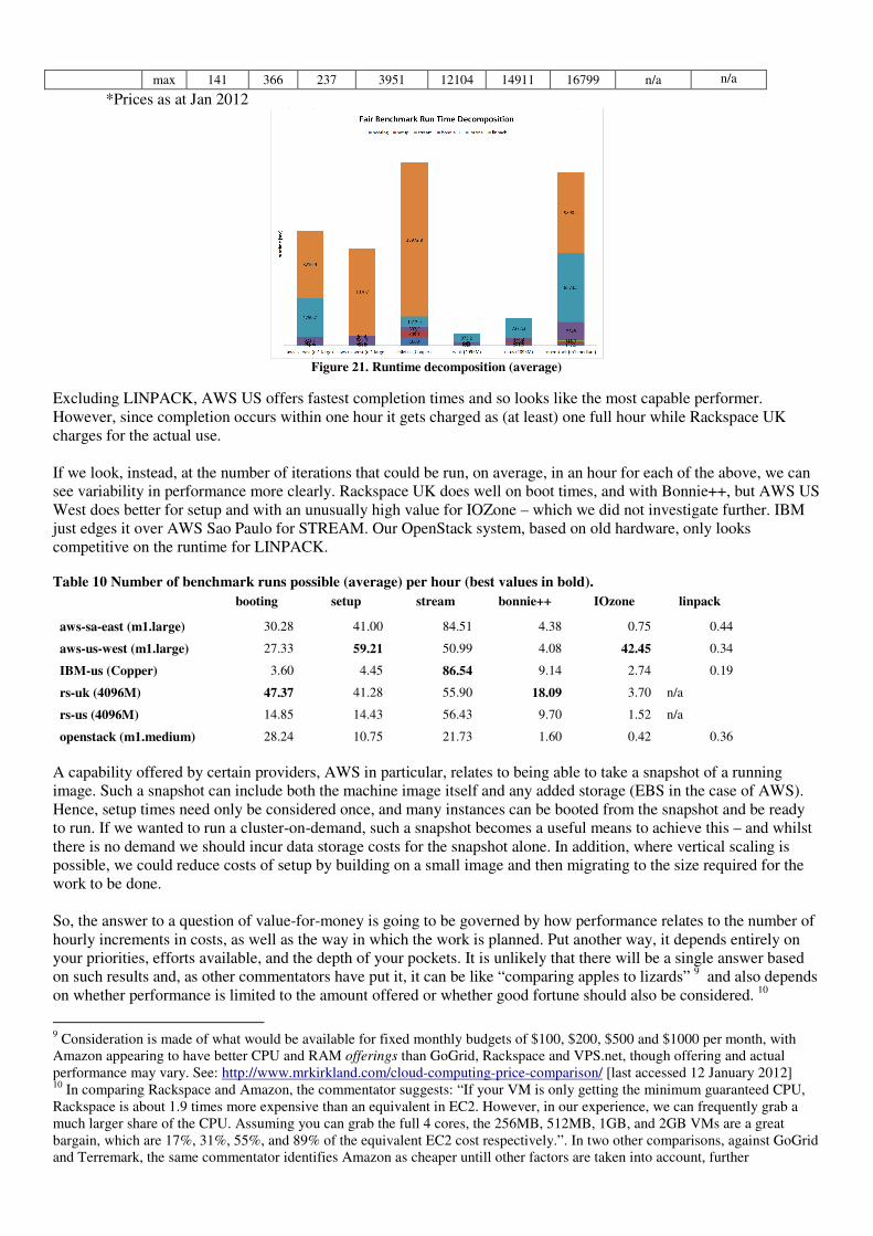
Figure 21. Runtime decomposition (average)

Excluding LINPACK, AWS US offers fastest completion times and so looks like the most capable performer. However, since completion occurs within one hour it gets charged as (at least) one full hour while Rackspace UK charges for the actual use. If we look, instead, at the number of iterations that could be run, on average, in an hour for each of the above, we can see variability in performance more clearly. Rackspace UK does well on boot times, and with Bonnie++, but AWS US West does better for setup and with an unusually high value for IOZone – which we did not investigate further. IBM just edges it over AWS Sao Paulo for STREAM. Our OpenStack system, based on old hardware, only looks competitive on the runtime for LINPACK.

Table 10 Number of benchmark runs possible (average) per hour (best values in bold).

booting setup stream bonnie++ IOzone linpack

aws-sa-east (m1.large) 30.28 41.00 84.51 4.38 0.75 0.44

aws-us-west (m1.large) 27.33 59.21 50.99 4.08 42.45 0.34

IBM-us (Copper) 3.60 4.45 86.54 9.14 2.74 0.19

rs-uk (4096M) 47.37 41.28 55.90 18.09 3.70 n/a

rs-us (4096M) 14.85 14.43 56.43 9.70 1.52 n/a

openstack (m1.medium) 28.24 10.75 21.73 1.60 0.42 0.36

A capability offered by certain providers, AWS in particular, relates to being able to take a snapshot of a running image. Such a snapshot can include both the machine image itself and any added storage (EBS in the case of AWS). Hence, setup times need only be considered once, and many instances can be booted from the snapshot and be ready to run. If we wanted to run a cluster-on-demand, such a snapshot becomes a useful means to achieve this – and whilst there is no demand we should incur data storage costs for the snapshot alone. In addition, where vertical scaling is possible, we could reduce costs of setup by building on a small image and then migrating to the size required for the work to be done. So, the answer to a question of value-for-money is going to be governed by how performance relates to the number of hourly increments in costs, as well as the way in which the work is planned. Put another way, it depends entirely on your priorities, efforts available, and the depth of your pockets. It is unlikely that there will be a single answer based on such results and, as other commentators have put it, it can be like “comparing apples to lizards” 9 and also depends on whether performance is limited to the amount offered or whether good fortune should also be considered. 10

9 Consideration is made of what would be available for fixed monthly budgets of $100, $200, $500 and $1000 per month, with Amazon appearing to have better CPU and RAM offerings than GoGrid, Rackspace and VPS.net, though offering and actual performance may vary. See: http://www.mrkirkland.com/cloud-computing-price-comparison/ [last accessed 12 January 2012] 10 In comparing Rackspace and Amazon, the commentator suggests: “If your VM is only getting the minimum guaranteed CPU, Rackspace is about 1.9 times more expensive than an equivalent in EC2. However, in our experience, we can frequently grab a much larger share of the CPU. Assuming you can grab the full 4 cores, the 256MB, 512MB, 1GB, and 2GB VMs are a great bargain, which are 17%, 31%, 55%, and 89% of the equivalent EC2 cost respectively.”. In two other comparisons, against GoGrid and Terremark, the same commentator identifies Amazon as cheaper untill other factors are taken into account, further

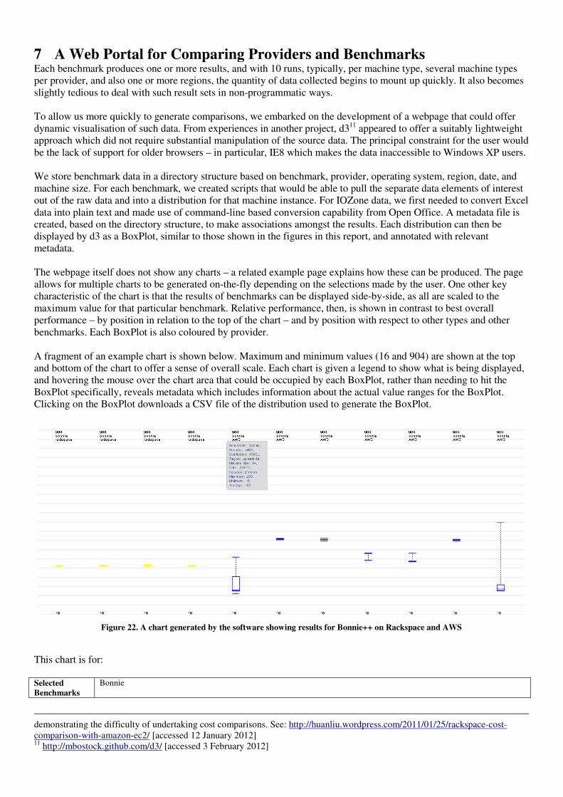
7 A Web Portal for Comparing Providers and Benchmarks Each benchmark produces one or more results, and with 10 runs, typically, per machine type, several machine types per provider, and also one or more regions, the quantity of data collected begins to mount up quickly. It also becomes slightly tedious to deal with such result sets in non-programmatic ways. To allow us more quickly to generate comparisons, we embarked on the development of a webpage that could offer dynamic visualisation of such data. From experiences in another project, d311 appeared to offer a suitably lightweight approach which did not require substantial manipulation of the source data. The principal constraint for the user would be the lack of support for older browsers – in particular, IE8 which makes the data inaccessible to Windows XP users. We store benchmark data in a directory structure based on benchmark, provider, operating system, region, date, and machine size. For each benchmark, we created scripts that would be able to pull the separate data elements of interest out of the raw data and into a distribution for that machine instance. For IOZone data, we first needed to convert Excel data into plain text and made use of command-line based conversion capability from Open Office. A metadata file is created, based on the directory structure, to make associations amongst the results. Each distribution can then be displayed by d3 as a BoxPlot, similar to those shown in the figures in this report, and annotated with relevant metadata. The webpage itself does not show any charts – a related example page explains how these can be produced. The page allows for multiple charts to be generated on-the-fly depending on the selections made by the user. One other key characteristic of the chart is that the results of benchmarks can be displayed side-by-side, as all are scaled to the maximum value for that particular benchmark. Relative performance, then, is shown in contrast to best overall performance – by position in relation to the top of the chart – and by position with respect to other types and other benchmarks. Each BoxPlot is also coloured by provider. A fragment of an example chart is shown below. Maximum and minimum values (16 and 904) are shown at the top and bottom of the chart to offer a sense of overall scale. Each chart is given a legend to show what is being displayed, and hovering the mouse over the chart area that could be occupied by each BoxPlot, rather than needing to hit the BoxPlot specifically, reveals metadata which includes information about the actual value ranges for the BoxPlot. Clicking on the BoxPlot downloads a CSV file of the distribution used to generate the BoxPlot.

Figure 22. A chart generated by the software showing results for Bonnie++ on Rackspace and AWS

This chart is for: Selected

Benchmarks

Bonnie

demonstrating the difficulty of undertaking cost comparisons. See: http://huanliu.wordpress.com/2011/01/25/rackspace-cost-comparison-with-amazon-ec2/ [accessed 12 January 2012] 11 http://mbostock.github.com/d3/ [accessed 3 February 2012]

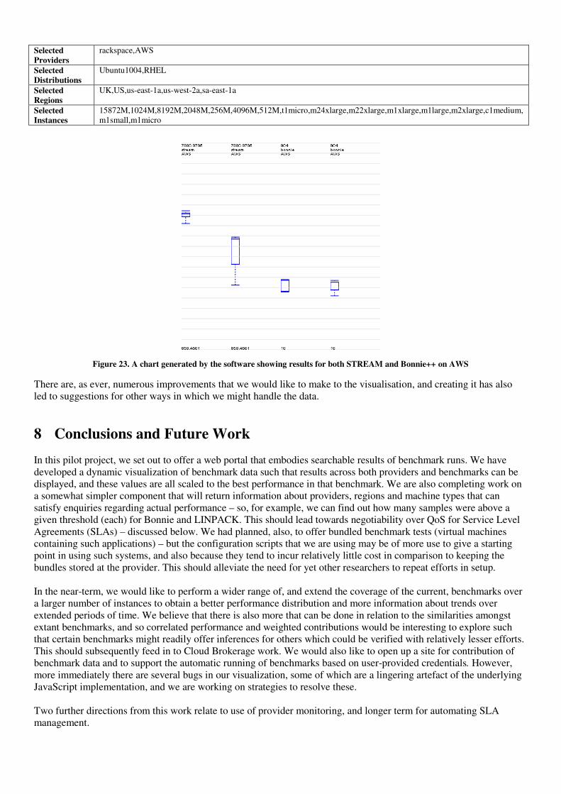
Selected

Providers

rackspace,AWS

Selected

Distributions

Ubuntu1004,RHEL

Selected

Regions

UK,US,us-east-1a,us-west-2a,sa-east-1a

Selected

Instances

15872M,1024M,8192M,2048M,256M,4096M,512M,t1micro,m24xlarge,m22xlarge,m1xlarge,m1large,m2xlarge,c1medium,m1small,m1micro

Figure 23. A chart generated by the software showing results for both STREAM and Bonnie++ on AWS

There are, as ever, numerous improvements that we would like to make to the visualisation, and creating it has also led to suggestions for other ways in which we might handle the data.

8 Conclusions and Future Work In this pilot project, we set out to offer a web portal that embodies searchable results of benchmark runs. We have developed a dynamic visualization of benchmark data such that results across both providers and benchmarks can be displayed, and these values are all scaled to the best performance in that benchmark. We are also completing work on a somewhat simpler component that will return information about providers, regions and machine types that can satisfy enquiries regarding actual performance – so, for example, we can find out how many samples were above a given threshold (each) for Bonnie and LINPACK. This should lead towards negotiability over QoS for Service Level Agreements (SLAs) – discussed below. We had planned, also, to offer bundled benchmark tests (virtual machines containing such applications) – but the configuration scripts that we are using may be of more use to give a starting point in using such systems, and also because they tend to incur relatively little cost in comparison to keeping the bundles stored at the provider. This should alleviate the need for yet other researchers to repeat efforts in setup. In the near-term, we would like to perform a wider range of, and extend the coverage of the current, benchmarks over a larger number of instances to obtain a better performance distribution and more information about trends over extended periods of time. We believe that there is also more that can be done in relation to the similarities amongst extant benchmarks, and so correlated performance and weighted contributions would be interesting to explore such that certain benchmarks might readily offer inferences for others which could be verified with relatively lesser efforts. This should subsequently feed in to Cloud Brokerage work. We would also like to open up a site for contribution of benchmark data and to support the automatic running of benchmarks based on user-provided credentials. However, more immediately there are several bugs in our visualization, some of which are a lingering artefact of the underlying JavaScript implementation, and we are working on strategies to resolve these. Two further directions from this work relate to use of provider monitoring, and longer term for automating SLA management.

8.1 Use of Amazon CloudWatch CloudWatch enables AWS users to set alarms for various metrics such as CPUUtilization (as a percentage), DiskReadBytes, DiskWriteBytes, NetworkIn, and NetworkOut, amongst others. The benchmarks we have explored are highly related to this set of metrics, and so it is immediately possible to consider how this would inform the setting of such alarms – although there would still be some effort needed on obtaining likely performance values per machine instance to begin with. An alarm can be set when one of these metrics is above or below a given value for longer than a specified period of time (in minutes). At present, unless an AutoScaling policy has been created, alarms will be sent by email.

8.2 Automating SLA management We have investigated the use of WS-Agreement in the automation of management of SLAs in this project and in prior work referred to earlier in this report. The latest WS-Agreement specification (1.0.0) helpfully separates out the static resource properties – such as amount of memory, numbers of CPUs, and so forth – from the dynamic resource properties – typically, limited to response times. The dynamic properties are those that can vary (continuously) over the agreement lifetime. WS-Agreement follows related contractual principles, allowing for the specification of the entities involved in the agreement, the work to be undertaken, and the conditions that relate to the performance of the contract. Initially, WS-Agreement consists of two sections: the Context, which defines properties of the agreement (i.e. name, date, parties of agreement); and the Terms, which are divided into Service Description Terms (SDTs) and Guarantee Terms (GTs). SDTs are used to identify the work to be done, describing, for example, the platform upon which the work is to be done, the software involved, and the set of expected arguments and input/output resources. GTs provide assurance between provider and requester on QoS, and should include the price of the service and, ideally, the probability of, and penalty for, failure. Introducing a Cloud Broker adds an element of complexity, although this may be beneficial. If users demand detailed SLAs but Cloud providers do not offer them, there is a clear advantage to the Broker if they can interpret/interrogate the resources in order to produce and manage such SLAs. ServiceQoS offers suggestions for how to add QoS parameters into SLAs12. The principal example is through a Key Performance Indicator (KPI) Target (wsag:KPITarget) as a Service Level Objective (wsag:ServiceLevelObjective), and relates to Response Time (wsag:KPIName). Examples elsewhere use Availability, and a threshold (e.g. gte 98.5, to indicate greater than or equal to 98.5%). Cloud providers and frameworks supporting this on a practical level are as yet not apparent, leaving the direct use of QoS parameters in SLAs for negotiation via Cloud Brokers very much on our future trajectory.

9 References [1] Cooper, B.F., Silberstein, A., Tam, E., Ramakrishnan, R., Sears, R. (2010), “Benchmarking cloud serving systems

with YCSB”, Proceedings of the 1st ACM symposium on Cloud computing, June 10-11, 2010, Indianapolis, Indiana, USA [doi>10.1145/1807128.1807152]

[2] Deacon, J. (2004). Global securitisation and CDOs (The Wiley Finance Series). Hoboken, NJ: John Wiley & Sons.

[3] Walker, E. (2008), “Benchmarking Amazon EC2 for high-performance scientific computing”, USENIX Login, vol. 33, no. 5, pp. 18–23, 2008.

[4] J D. McCalpin, "STREAM: Sustainable Memory Bandwidth in High Performance Computers", a continually updated technical report (1991-2007), available at: "http://www.cs.virginia.edu/stream/".

[5] Gray, J. (ed.) (1993), “The Benchmark Handbook For Database and Transaction Processing Systems”. Morgan Kaufmann.

[6] Napper, J. and Bientinesi, P. (2009), “Can cloud computing reach the top500?”. Proc. of the combined workshops on UnConventional high performance computing workshop plus memory access workshop pp17-20, ACM.

[7] Jorion, P., & GARP (Global Association of Risk Professionals). (2007). Financial Risk Manager Handbook (Wiley Finance) (4th Ed.). Hoboken, NJ: John Wiley & Sons.

12 ServiceQoS: http://serviceqos.wikispaces.com/WSAgExample [accessed 3 February 2012]

[8] Jackson, K.R., Ramakrishnan, L., Muriki, K., Canon, S., Cholia, S., Shalf, J., Wasserman, H.J., Wright, N.J. (2010), "Performance Analysis of High Performance Computing Applications on the Amazon Web Services Cloud", Proc. CloudCom 2010, pp159 – 168.

[9] Li, B., Gillam, L., and O'Loughlin, J. (2010) Towards Application-Specific Service Level Agreements: Experiments in Clouds and Grids, In Antonopoulos and Gillam (Eds.), Cloud Computing: Principles, Systems and Applications. Springer-Verlag.

[10] Li, B., and Gillam, L. (2009), Towards Job-specific Service Level Agreements in the Cloud, Cloud-based Services and Applications, in 5th IEEE e-Science International Conference, Oxford, UK.

[11] Li, B., and Gillam, L. (2009), Grid Service Level Agreements using Financial Risk Analysis Techniques, In Antonopoulos, Exarchakos, Li and Liotta (Eds.), Handbook of Research on P2P and Grid Systems for Service-Oriented Computing: Models, Methodologies and Applications. IGI Global.

[12] Sion, R. and colleagues, Cloud Performance Benchmark Series, available at http://www.cs.sunysb.edu/~sion/research/ (Jan2012)

[13] Tavakoli, M. J. (2003). Collateralized Debt Obligations & Structured Finance: New Developments in Cash and Synthetic Securitization (2nd Ed.). Hoboken, NJ: John Wiley & Sons.

9.1 Relevant Websites – accessed 3 February 2012 [14] Yahoo! Cloud Serving Benchmark project, http://research.yahoo.com/Web_Information_Management/YCSB [15] Amazon Web Services, EC2, S3, http://aws.amazon.com/ [16] Rackspace, http://www.rackspace.com/ [17] IBM SmartCloud, http://www.ibm.com/cloud-computing/us/en/ ; https://www-

147.ibm.com/cloud/enterprise/dashboard [18] Openstack, http://www.openstack.org/ [19] NewServers: Bare Metal Cloud, http://www.newservers.com/language/en/ [20] Apache libcloud. http://libcloud.apache.org/ [21] Jclouds, http://www.jclouds.org/ [22] DeltaCloud, http://www.jclouds.org/ [23] STREAM, http://www.cs.virginia.edu/stream/ [24] Bonnie++, http://www.coker.com.au/bonnie++/ [25] Iozone, http://www.iozone.org/ [26] Linpack, http://software.intel.com/en-us/articles/intel-linpack-benchmark-download-license-agreement/ [27] Iperf, http://iperf.sourceforge.net/ [28] MPPTEST, http://www.mcs.anl.gov/research/projects/mpi/mpptest/ [29] Bzip2, http://bzip.org/; http://www.spec.org/cpu2006/Docs/401.bzip2.html ; http://www.phoronix-test-

suite.com/ [30] Cloudharmony, http://cloudharmony.com/ [31] CLOUDSLEUTH, https://cloudsleuth.net/ [32] Openbenchmarking, http://openbenchmarking.org/ [33] Shopping the Cloud: Performance Benchmarks http://gevaperry.typepad.com/main/2010/08/shopping-the-

cloud-performance-benchmarks.html [34] Amazon EC2 Cloud Benchmarks,

http://www.phoronix.com/scan.php?page=article&item=amazon_ec2_round1&num=1 [35] Amazon EC2 Micro: Barely Faster Than A Nokia N900?

http://www.phoronix.com/scan.php?page=article&item=amazon_ec2_micro&num=1 [36] Disk IO and throughput benchmarks on Amazon’s EC2, http://stu.mp/2009/12/disk-io-and-throughput-

benchmarks-on-amazons-ec2.html [37] Comparing a traditional cluster with Amazon’s EC2 on the NAS benchmarks and Linpack,

http://insidehpc.com/2009/08/03/comparing-hpc-cluster-amazons-ec2-nas-benchmarks-linpack/ [38] EC2 CPU benchmark: Fastest instance type (serial performance)

http://opinionatedprogrammer.com/2011/07/ec2-cpu-benchmark-fastest-instance-type-for-build-servers/ [39] IOzone benchmark vs EC2, http://blog.dbadojo.com/2007/10/iozone-benchmark-vs-ec2.html

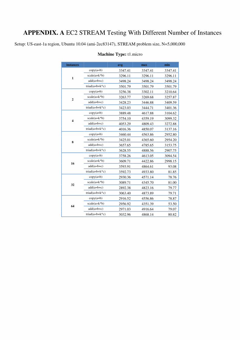
APPENDIX. A EC2 STREAM Testing With Different Number of Instances Setup: US-east-1a region, Ubuntu 10.04 (ami-2ec83147), STREAM problem size, N=5,000,000

Machine Type: t1.micro

instances avg max min

1

copy(a=b) 3347.41 3347.41 3347.41

scale(a=k*b) 3296.11 3296.11 3296.11

add(a=b+c) 3498.24 3498.24 3498.24

triad(a=b+k*c) 3501.79 3501.79 3501.79

2

copy(a=b) 3256.38 3302.11 3210.64

scale(a=k*b) 3263.77 3269.68 3257.87

add(a=b+c) 3428.23 3446.88 3409.59

triad(a=b+k*c) 3423.03 3444.71 3401.36

4

copy(a=b) 3889.48 4617.88 3104.62

scale(a=k*b) 3754.10 4359.19 3099.32

add(a=b+c) 4053.29 4809.43 3272.88

triad(a=b+k*c) 4016.36 4850.07 3137.16

8

copy(a=b) 3460.44 4563.86 2952.80

scale(a=k*b) 3425.01 4365.60 2954.20

add(a=b+c) 3657.65 4785.65 3153.75

triad(a=b+k*c) 3628.55 4888.56 2907.75

16

copy(a=b) 3758.26 4613.05 3094.54

scale(a=k*b) 3609.71 4422.86 2998.15

add(a=b+c) 3593.91 4864.61 93.08

triad(a=b+k*c) 3592.73 4933.80 81.85

32

copy(a=b) 2930.36 4571.14 78.76

scale(a=k*b) 3089.71 4345.70 81.00

add(a=b+c) 2892.38 4823.16 79.77

triad(a=b+k*c) 3063.40 4873.89 79.71

64

copy(a=b) 2916.52 4556.86 78.87

scale(a=k*b) 2956.92 4351.39 53.50

add(a=b+c) 2971.03 4916.64 79.07

triad(a=b+k*c) 3032.96 4868.14 80.82

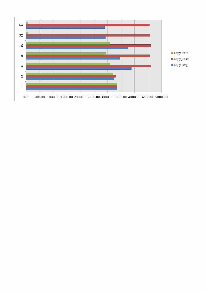
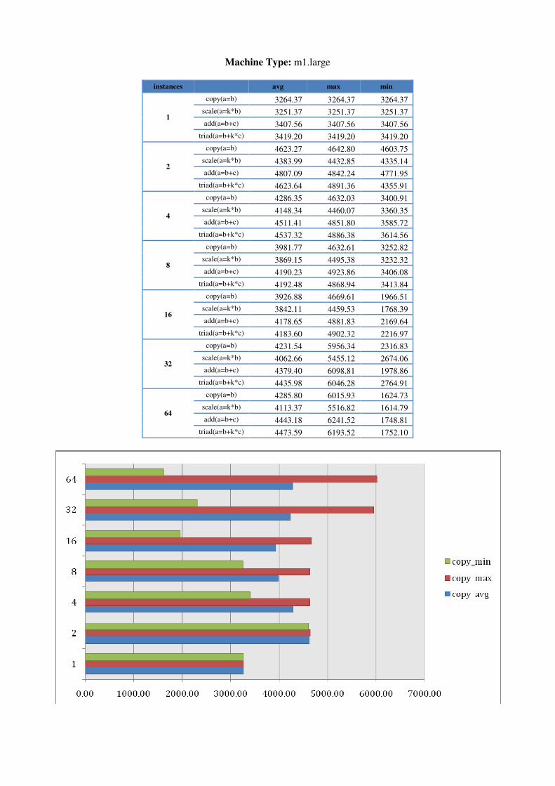
Machine Type: m1.large

instances avg max min

1

copy(a=b) 3264.37 3264.37 3264.37

scale(a=k*b) 3251.37 3251.37 3251.37

add(a=b+c) 3407.56 3407.56 3407.56

triad(a=b+k*c) 3419.20 3419.20 3419.20

2

copy(a=b) 4623.27 4642.80 4603.75

scale(a=k*b) 4383.99 4432.85 4335.14

add(a=b+c) 4807.09 4842.24 4771.95

triad(a=b+k*c) 4623.64 4891.36 4355.91

4

copy(a=b) 4286.35 4632.03 3400.91

scale(a=k*b) 4148.34 4460.07 3360.35

add(a=b+c) 4511.41 4851.80 3585.72

triad(a=b+k*c) 4537.32 4886.38 3614.56

8

copy(a=b) 3981.77 4632.61 3252.82

scale(a=k*b) 3869.15 4495.38 3232.32

add(a=b+c) 4190.23 4923.86 3406.08

triad(a=b+k*c) 4192.48 4868.94 3413.84

16

copy(a=b) 3926.88 4669.61 1966.51

scale(a=k*b) 3842.11 4459.53 1768.39

add(a=b+c) 4178.65 4881.83 2169.64

triad(a=b+k*c) 4183.60 4902.32 2216.97

32

copy(a=b) 4231.54 5956.34 2316.83

scale(a=k*b) 4062.66 5455.12 2674.06

add(a=b+c) 4379.40 6098.81 1978.86

triad(a=b+k*c) 4435.98 6046.28 2764.91

64

copy(a=b) 4285.80 6015.93 1624.73

scale(a=k*b) 4113.37 5516.82 1614.79

add(a=b+c) 4443.18 6241.52 1748.81

triad(a=b+k*c) 4473.59 6193.52 1752.10

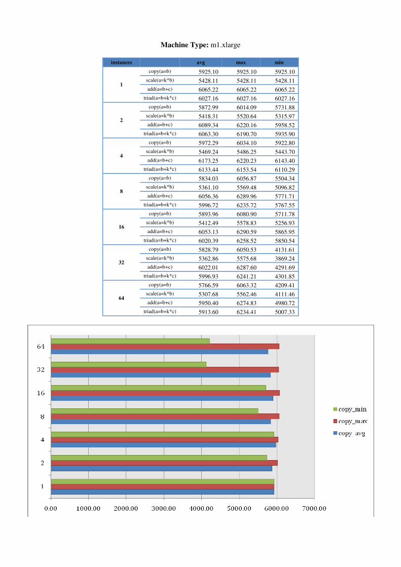
Machine Type: m1.xlarge

instances avg max min

1

copy(a=b) 5925.10 5925.10 5925.10

scale(a=k*b) 5428.11 5428.11 5428.11

add(a=b+c) 6065.22 6065.22 6065.22

triad(a=b+k*c) 6027.16 6027.16 6027.16

2

copy(a=b) 5872.99 6014.09 5731.88

scale(a=k*b) 5418.31 5520.64 5315.97

add(a=b+c) 6089.34 6220.16 5958.52

triad(a=b+k*c) 6063.30 6190.70 5935.90

4

copy(a=b) 5972.29 6034.10 5922.80

scale(a=k*b) 5469.24 5486.25 5443.70

add(a=b+c) 6173.25 6220.23 6143.40

triad(a=b+k*c) 6133.44 6153.54 6110.29

8

copy(a=b) 5834.03 6056.87 5504.34

scale(a=k*b) 5361.10 5569.48 5096.82

add(a=b+c) 6056.36 6289.96 5771.71

triad(a=b+k*c) 5996.72 6235.72 5767.55

16

copy(a=b) 5893.96 6080.90 5711.78

scale(a=k*b) 5412.49 5578.83 5256.93

add(a=b+c) 6053.13 6290.59 5865.95

triad(a=b+k*c) 6020.39 6258.52 5850.54

32

copy(a=b) 5828.79 6050.53 4131.61

scale(a=k*b) 5362.86 5575.68 3869.24

add(a=b+c) 6022.01 6287.60 4291.69

triad(a=b+k*c) 5996.93 6241.21 4301.85

64

copy(a=b) 5766.59 6063.32 4209.41

scale(a=k*b) 5307.68 5562.46 4111.46

add(a=b+c) 5950.40 6274.83 4980.72

triad(a=b+k*c) 5913.60 6234.41 5007.33

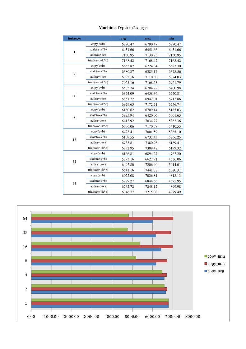
Machine Type: m2.xlarge

instances avg max min

1

copy(a=b) 6790.47 6790.47 6790.47

scale(a=k*b) 6451.66 6451.66 6451.66

add(a=b+c) 7130.95 7130.95 7130.95

triad(a=b+k*c) 7168.42 7168.42 7168.42

2

copy(a=b) 6653.82 6724.34 6583.30

scale(a=k*b) 6380.87 6383.17 6378.56

add(a=b+c) 6992.16 7110.30 6874.03

triad(a=b+k*c) 7065.16 7168.53 6961.79

4

copy(a=b) 6585.74 6704.72 6460.98

scale(a=k*b) 6324.09 6458.36 6220.81

add(a=b+c) 6851.72 6942.01 6712.86

triad(a=b+k*c) 6979.63 7172.71 6756.74

8

copy(a=b) 6180.62 6709.14 5185.03

scale(a=k*b) 5995.94 6420.06 5001.63

add(a=b+c) 6413.92 7034.77 5362.36

triad(a=b+k*c) 6556.06 7170.57 5410.55

16

copy(a=b) 6423.41 7001.59 5365.10

scale(a=k*b) 6109.55 6737.43 5266.25

add(a=b+c) 6733.81 7380.98 6189.41

triad(a=b+k*c) 6732.95 7309.48 6199.32

32

copy(a=b) 6166.81 6894.27 4762.20

scale(a=k*b) 5893.16 6627.91 4636.06

add(a=b+c) 6492.80 7206.40 5014.01

triad(a=b+k*c) 6541.16 7441.88 5020.31

64

copy(a=b) 6022.08 7026.81 4818.13

scale(a=k*b) 5729.27 6844.63 4695.95

add(a=b+c) 6262.72 7248.12 4899.98

triad(a=b+k*c) 6346.77 7215.08 4979.49

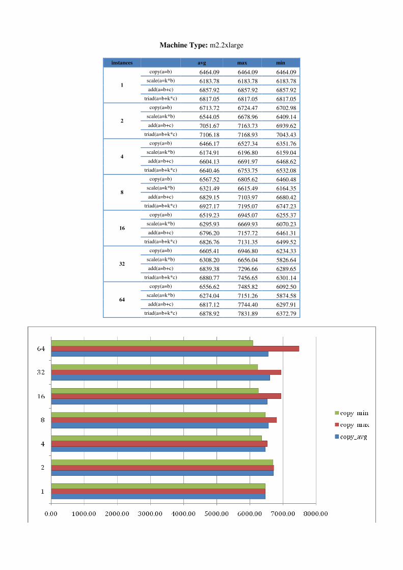
Machine Type: m2.2xlarge

instances avg max min

1

copy(a=b) 6464.09 6464.09 6464.09

scale(a=k*b) 6183.78 6183.78 6183.78

add(a=b+c) 6857.92 6857.92 6857.92

triad(a=b+k*c) 6817.05 6817.05 6817.05

2

copy(a=b) 6713.72 6724.47 6702.98

scale(a=k*b) 6544.05 6678.96 6409.14

add(a=b+c) 7051.67 7163.73 6939.62

triad(a=b+k*c) 7106.18 7168.93 7043.43

4

copy(a=b) 6466.17 6527.34 6351.76

scale(a=k*b) 6174.91 6196.80 6159.04

add(a=b+c) 6604.13 6691.97 6468.62

triad(a=b+k*c) 6640.46 6753.75 6532.08

8

copy(a=b) 6567.52 6805.62 6460.48

scale(a=k*b) 6321.49 6615.49 6164.35

add(a=b+c) 6829.15 7103.97 6680.42

triad(a=b+k*c) 6927.17 7195.07 6747.23

16

copy(a=b) 6519.23 6945.07 6255.37

scale(a=k*b) 6295.93 6669.93 6070.23

add(a=b+c) 6796.20 7157.72 6461.31

triad(a=b+k*c) 6826.76 7131.35 6499.52

32

copy(a=b) 6605.41 6946.80 6234.33

scale(a=k*b) 6308.20 6656.04 5826.64

add(a=b+c) 6839.38 7296.66 6289.65

triad(a=b+k*c) 6880.77 7456.65 6301.14

64

copy(a=b) 6556.62 7485.82 6092.50

scale(a=k*b) 6274.04 7151.26 5874.58

add(a=b+c) 6817.12 7744.40 6297.91

triad(a=b+k*c) 6878.92 7831.89 6372.79

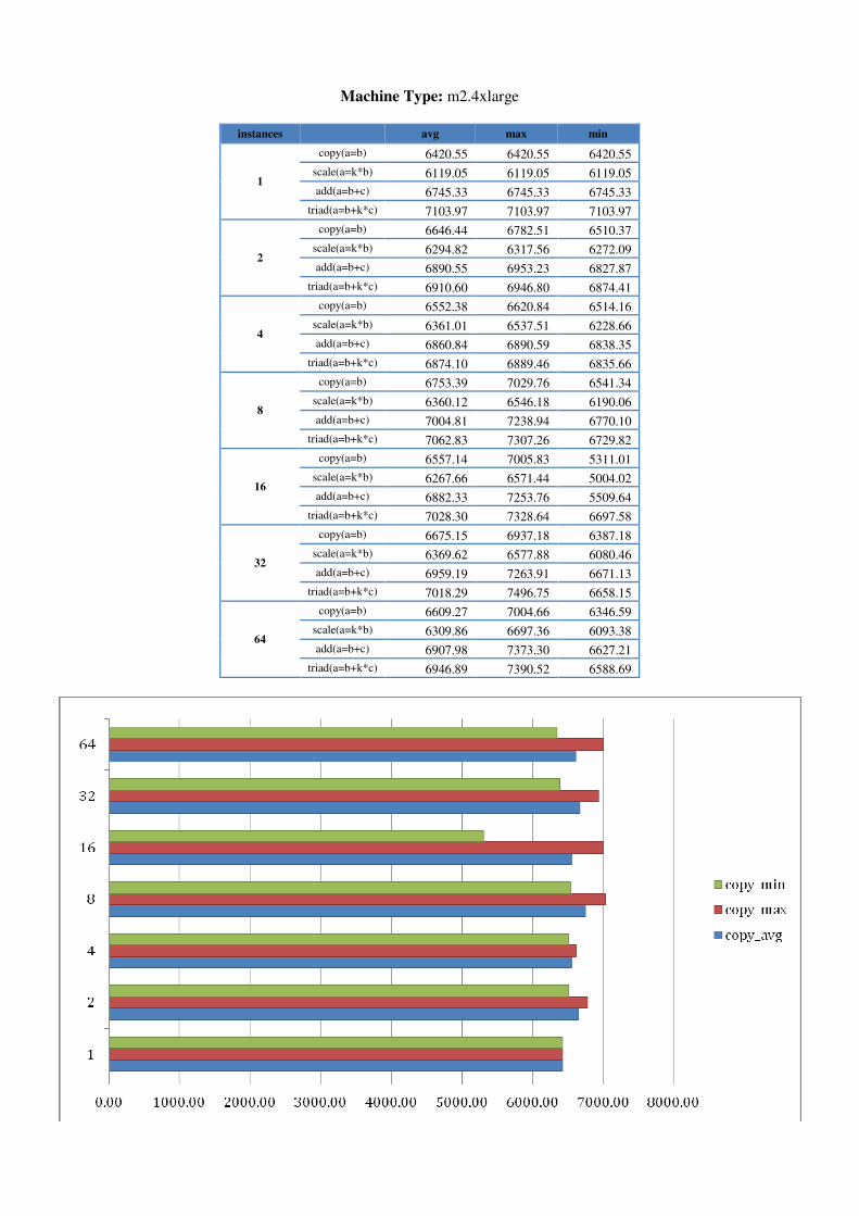
Machine Type: m2.4xlarge

instances avg max min

1

copy(a=b) 6420.55 6420.55 6420.55

scale(a=k*b) 6119.05 6119.05 6119.05

add(a=b+c) 6745.33 6745.33 6745.33

triad(a=b+k*c) 7103.97 7103.97 7103.97

2

copy(a=b) 6646.44 6782.51 6510.37

scale(a=k*b) 6294.82 6317.56 6272.09

add(a=b+c) 6890.55 6953.23 6827.87

triad(a=b+k*c) 6910.60 6946.80 6874.41

4

copy(a=b) 6552.38 6620.84 6514.16

scale(a=k*b) 6361.01 6537.51 6228.66

add(a=b+c) 6860.84 6890.59 6838.35

triad(a=b+k*c) 6874.10 6889.46 6835.66

8

copy(a=b) 6753.39 7029.76 6541.34

scale(a=k*b) 6360.12 6546.18 6190.06

add(a=b+c) 7004.81 7238.94 6770.10

triad(a=b+k*c) 7062.83 7307.26 6729.82

16

copy(a=b) 6557.14 7005.83 5311.01

scale(a=k*b) 6267.66 6571.44 5004.02

add(a=b+c) 6882.33 7253.76 5509.64

triad(a=b+k*c) 7028.30 7328.64 6697.58

32

copy(a=b) 6675.15 6937.18 6387.18

scale(a=k*b) 6369.62 6577.88 6080.46

add(a=b+c) 6959.19 7263.91 6671.13

triad(a=b+k*c) 7018.29 7496.75 6658.15

64

copy(a=b) 6609.27 7004.66 6346.59

scale(a=k*b) 6309.86 6697.36 6093.38

add(a=b+c) 6907.98 7373.30 6627.21

triad(a=b+k*c) 6946.89 7390.52 6588.69