fan surging

©2004 ASHRAE. 347

ABSTRACT

This paper describes the development and testing of thecharacteristic curve fan model—a gray-box model. This modelproduces fan efficiency as a function of airflow and fan staticpressure. It is accurate, relatively easy to calibrate, and couldbe easily incorporated into commercial simulation programs.Also presented is an application of an existing model to predictfan speed from airflow and fan static pressure. These modelswere developed as a part of a larger research project to developdesign guidelines for built-up variable air volume fan systems.The models have been successfully employed in comparativeanalysis of fan types, wheel diameters, fan staging, and anal-ysis of supply pressure reset.

INTRODUCTION

The authors were part of a publicly funded energy effi-ciency research team developing design guidelines for built-up fan systems in commercial buildings. According to previ-ous research, fan energy in new construction for commercialbuildings in California accounts for 1 terawatt-hour of electricenergy usage per year, representing approximately half of allHVAC energy usage (CALMAC 2003). The authors’ researchdemonstrates that up to half of that fan energy is avoidablethrough cost-effective design practices, including fan selec-tion (size and type), fan sizing, fan staging, and static pressurecontrol (Hydeman and Stein 2003). Five monitoring sitesprovided field data on which to test the alternative fan systemdesigns and design techniques. These sites were selected torepresent a range of climates, occupancies, and fan systemconfigurations (Kolderup et al. 2002). As part of this work, asimulation model of a fan system was sought that had all of thefollowing characteristics:

• Accurate at predicting fan system energy over the fullrange of actual or anticipated operating conditions.

• Applicable for the full range of fan types and sizes.• Easy to calibrate from manufacturer’s or field-moni-

tored data.• Ability to identify operation in the “surge” region.• Relatively simple to integrate into existing simulation

tools.• Ability to independently model the performance of the

fan system components, including the motor, themechanical drive components, the unloading mecha-nism (e.g., VSD), and the fan.

The purpose of this model is to evaluate design alterna-tives for fan selection and control through simulation. Opti-mally, simulation tools would directly utilize themanufacturers’ fan curves to evaluate fan system operation ateach discrete step of evaluation. Since this is not currentlyavailable, the authors sought models that simulation toolscould easily incorporate that replicated fan performance.

MAIN BODY

Literature on component models for fans was reviewed,including the models used in the DOE-2 simulation program(DOE 1980) and in the ASHRAE Secondary Toolkit (Bran-demuehl et al. 1993; Clark, 1985). We also looked briefly atthe models embedded in commercial simulation software,such as Trace and HAP, but found these suffered from the sameproblems as the model in DOE-2.

DOE-2 uses a black-box regression model that producesthe fan system power draw as a function of percent designairflow using a second-order equation as follows:

Development and Testing of theCharacteristic Curve Fan Model

Jeff Stein, P.E. Mark M. Hydeman, P.E.Member ASHRAE Member ASHRAE

Jeff Stein is a senior engineer and Mark Hydeman is a principal at Taylor Engineering, LLC, Alameda, Calif.

AN-04-3-1

348 ASHRAE Transactions: Symposia

(1)

This model is implicitly built on several assumptions:

1. Each fan operates on a single system curve that uniquelymaps airflow to static pressure.

2. Fan system efficiency is directly a function of airflow.

3. A second-order equation sufficiently models both of theseeffects.

The DOE fan model implicitly combines the operatingsystem curve with the models for each of the fan systemcomponents. Power is directly produced as a function ofairflow only, and there is no opportunity to have differentconditions of fan static pressure at a given airflow. Real VAVsystems do not remain on a fixed system curve. System pres-sure as a function of airflow behaves differently depending onthe location of the boxes that are modulating, the location ofthe static pressure sensor(s), and the static pressure controlalgorithm.

Although this model is simple to use, it does not allow theuser to independently model and evaluate each of the fan-system components. Thus, if designers wanted to evaluate theimpact of motor oversizing, they would have to independentlyassemble fan and motor models to develop the DOE-2 perfor-mance curve that represented the combination of the twotogether. This model also does not directly account for thevariation in fan system component efficiencies as the fanunloads, nor does it allow for evaluation of a multiple fansystem, where fan staging will change both the operating effi-ciency and potentially the individual fan static as they arestaged on and off.

The model in the ASHRAE Secondary Toolkit is a gray-box fan component model that uses the perfect fan lawsthrough application of dimensionless flow (φ) and pressure(ψ) coefficients. This model uses a fourth-order equation topredict fan efficiency from the dimensionless flow parameter.

(2)

(3)

(4)

where

CFM = airflow

N = fan speed

D = fan diameter

ρ = average air density

∆P = fan static pressure and

C1 and C2 = constants that make the coefficients dimensionless

This model allows the user to calibrate an entire family offan curves with data from a single model. Unfortunately, thismodel does not permit the direct calculation of fan efficiencyfrom airflow and pressure; rather, it correlates efficiency to thedimensionless flow term (φ), which requires both airflow andfan speed as inputs. As elaborated below, a designer (and mostsimulation tools) will use airflow and fan pressure as inputs tothe fan system model in order to calculate fan speed and effi-ciency. A second problem is that this model assumes a fixedpeak efficiency for fans of all sizes. This simplificationreduces the applicability of the fan model for comparativeanalysis of fan options as peak efficiency tends to increasewith fan diameter.

As a result of these shortcomings, the authors set out todevelop a new component model that could directly be drivenby airflow and pressure. Based on the “fan laws” (ASHRAE2000), the core assumption of this new “characteristic curve”fan model is that the efficiency of a fan is constant as the fanrides up and down on a particular characteristic system curve.Extensive testing with manufacturers’ fan selection softwaredemonstrates that the manufacturers also use this simplifyingassumption for developing fan performance data in both thesurge and non-surge regions. ANSI/ASHRAE Standard 51-1999 (ANSI/AMCA Standard 210-99) (ASHRAE 1999)explicitly permits this. For this model, a “characteristic systemcurve” is defined as a second-order equation, equating fanstatic pressure to airflow (cfm) with a zero constant and nofirst-order coefficient. For example, a VAV supply fan with afixed duct static pressure setpoint of 1.5 in. w.c. will ride upand down on a system curve that runs through the design pointand through 1.5 in. at 0 CFM. A “characteristic system curve”is a particular type of system curve in that it must run throughthe origin (0 in. at 0 CFM). A characteristic system curve ischaracterized by a single coefficient, SCC (system curve coef-ficient). The equation for any characteristic system curve is

(5)

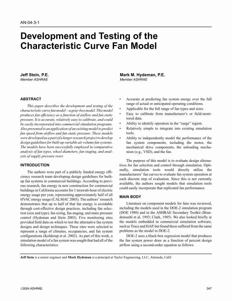
Using this assumption, it is only necessary to find fanperformance at a single point on a characteristic system curveto define its performance along that curve at all speeds. Asdepicted in Figure 1, there are three characteristic systemcurves of particular importance: the curves at the minimumand maximum ends of the tuning data set and the curve thatrepresents the highest efficiency for the fan. As describedbelow and depicted in Figure 3, fans behave very differently oneither side of this peak efficiency. The minimum and maxi-mum curves represent the boundaries of the model tuning data.

The triangles in Figure 1 depict points of data that weresampled from the manufacturer’s fan selection software. Eachpoint represents the fan efficiency for all points on a charac-teristic system curve. The fan efficiency is calculated from thefan brake horsepower (BHP), airflow (CFM), and fan staticpressure (∆P) reported by the software through the followingequation:

P

Pdesign

----------------- a b+CFM

CFMdesign

---------------------------⎝ ⎠⎛ ⎞× c+

CFM

CFMdesign

---------------------------⎝ ⎠⎛ ⎞ 2×=

φ c1

CFM

N D3

×-----------------×=

ψ c2

P∆

ρ N2

× D2

×-----------------------------×=

ηfan a b+ φ× c+ φ2

× d+ φ3

× e+ φ4

×=

SCCP∆

CFM2

--------------- .=

ASHRAE Transactions: Symposia 349

(6)

The model can be used to predict the fan power for anypoint whose system curve is between the two extreme systemcurves. Figure 1 is overlaid on top of an output screen from amanufacturer’s selection program. Notice that the peak effi-ciency line is also the boundary of the manufacturer’s “Do NotSelect” or surge region. This is typical for plenum, backwardinclined, and vane-axial fans. For airfoil, mixed flow, andpropeller fans, the peak efficiency is well to the right (i.e.,outside) of the surge region (see Figure 5).

When a fan enters the surge region, not only does the effi-ciency drop, but also the fan begins to vibrate, which can createaudible noise and damage the fan, bearings, drive, andattached ductwork. The further the fan moves into the surgeregion, the greater the vibration. Catastrophic failure canoccur if the fan moves well into the surge region at high power(high static). Some manufacturers appear to be more conser-vative than others in terms of what amount of vibration isacceptable. Moving into the surge region at low power (lowstatic) is not likely to cause catastrophic failure or unaccept-able vibration, but it will reduce fan life. From our experience,fans with variable-speed drives commonly operate forextended periods of time in the surge region, but it is usuallyat low power.

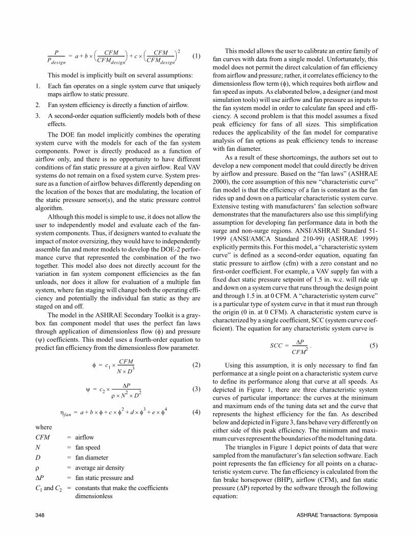
Figure 2 shows fan efficiency plotted against systemcurve coefficient (SCC) for the data from this 66 in. plenumfan. The efficiency data naturally divide into two regions—leftand right of the peak efficiency. It is interesting to note that thesurge region in Figure 2 is to the right of peak efficiency,whereas it is to the left in the manufacturer’s fan curve (Figure1). The representation in Figure 2 is also somewhat hard toread, as it condenses the normal region to a small space.

The efficiency curve is easier to visualize and to fit aregression equation if plotted as a function of the negative ofthe log of the system curve coefficient (see Figure 3). The logcauses the efficiency curves to become nearly linear, and thenegative flips the surge and normal regions so that it matchesmanufacturer’s curves (i.e., surge to the left, normal operationto the right). The base of the log does not seem to make muchdifference. Natural log is used here. Gamma is defined as thenegative of the natural log of the system curve coefficient.

ηfan

CFM P∆×6350 BHP×------------------------------=

Figure 1 Tuning data for 66 in. plenum fan shown on amanufacturer’s fan curve.

Figure 2 Fan efficiency vs. system curve coefficient.


(7)

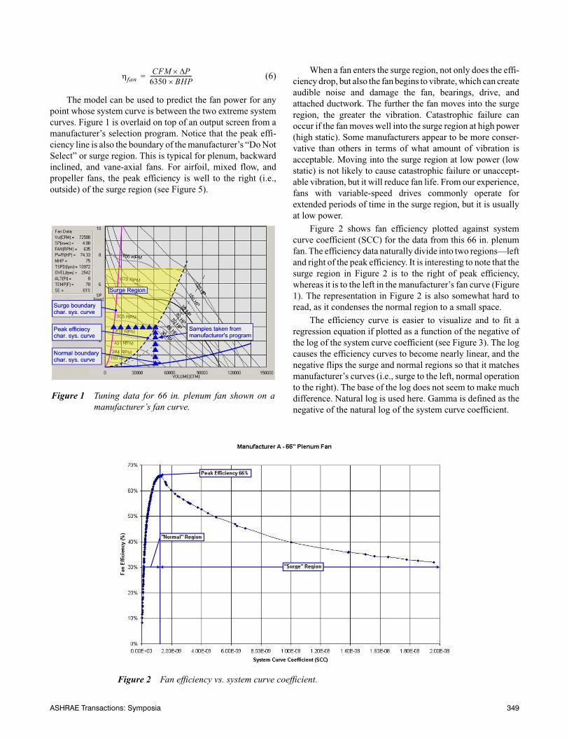
Fan efficiency can be accurately predicted as a function ofgamma. The recommended procedure is to break the functioninto two parts: an equation for gammas in the “surge” regionand another for gammas in the “normal” region. For thisreason, it is important to get an accurate indication of the “crit-ical gamma,” which is the gamma that corresponds to thesystem curve of highest fan efficiency. This can be done withthe manufacturer’s software by iterating on the airflow condi-tions in the vicinity of the critical gamma.

Figure 3 shows the R-square regression statistic for vari-ous orders of polynomials to the example 66 in. plenum fan.As demonstrated in Figure 3, a first-order polynomial (i.e.,straight line) is reasonably accurate. Higher order polynomialsprovide a better fit, but they require more data to calibrate andcan produce undesirable results between calibration datapoints. A third-order regression appears to provide a goodbalance between calibration accuracy to the tuning data setand rational function behavior between calibrating datapoints. These equations are of the form:

(8)

(9)

where S0…S3 and N0…N3 are regression coefficients devel-

oped from tuning data on the left (surge) side and right(normal) side of the peak efficiency point.

Regardless of the equation order, care must be taken toprovide a continuous function through the critical gammapoint.

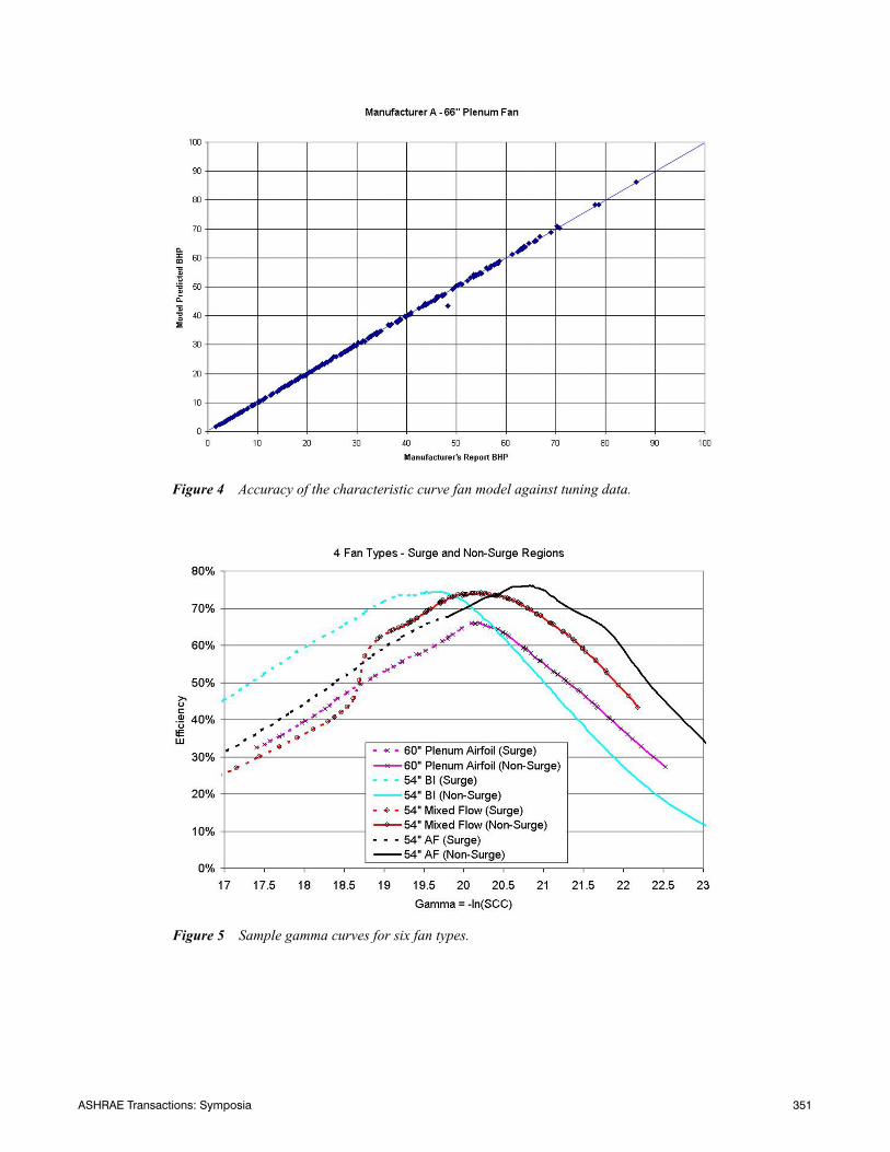
Figure 4 shows the accuracy of the characteristic curvefan model across 224 points, representing a wide range of fanspeeds, pressures, and airflows. This tuning data came from amanufacturer’s selection program, and the results arepresented against this tuning data set. We used third-orderpolynomials to represent efficiency of gamma, with separateequations in the “surge” and “normal” regions (Equations 8and 9).

The characteristic curve model has been found to be accu-rate for at least six types of fans: plenum, backward inclined,airfoil, mixed flow, propeller, and vane-axial with fixedblades. This model does not apply to fans with variable pitchblades or inlet vanes. Figure 5 shows sample gamma curves forfour types of fans. The curves are divided into the surge andnon-surge regions in order to illustrate the relationshipbetween peak efficiency and the surge region.

Table 1 presents the characteristic curve fan model fitresults across a range of manufacturers and fan types (plenumand housed, airfoil, and flat blade) and wheel diameters. Thistable presents the coefficient of variation root mean squareerror (CVRMSE) across the 57 fans in the database. Again,this represents third-order polynomial fits against tuning datafrom manufacturer’s selection programs. Typically a fit of 1%to 3% CVRMSE is excellent; a 5% fit is acceptable. Table 1

γ SCC( )ln–≡

Figure 3 Fan efficiency as a function of gamma.

ηfan_left_of_peak_efficiency S0 S1+ γ× S2+ γ2

× S3+ γ3

×=

ηfan_right_of_peak_efficiency N0 N1+ γ× N2+ γ2

× N3+ γ3

×=


Figure 4 Accuracy of the characteristic curve fan model against tuning data.

Figure 5 Sample gamma curves for six fan types.


shows that the average CVRMSE is well within the excellentregion.

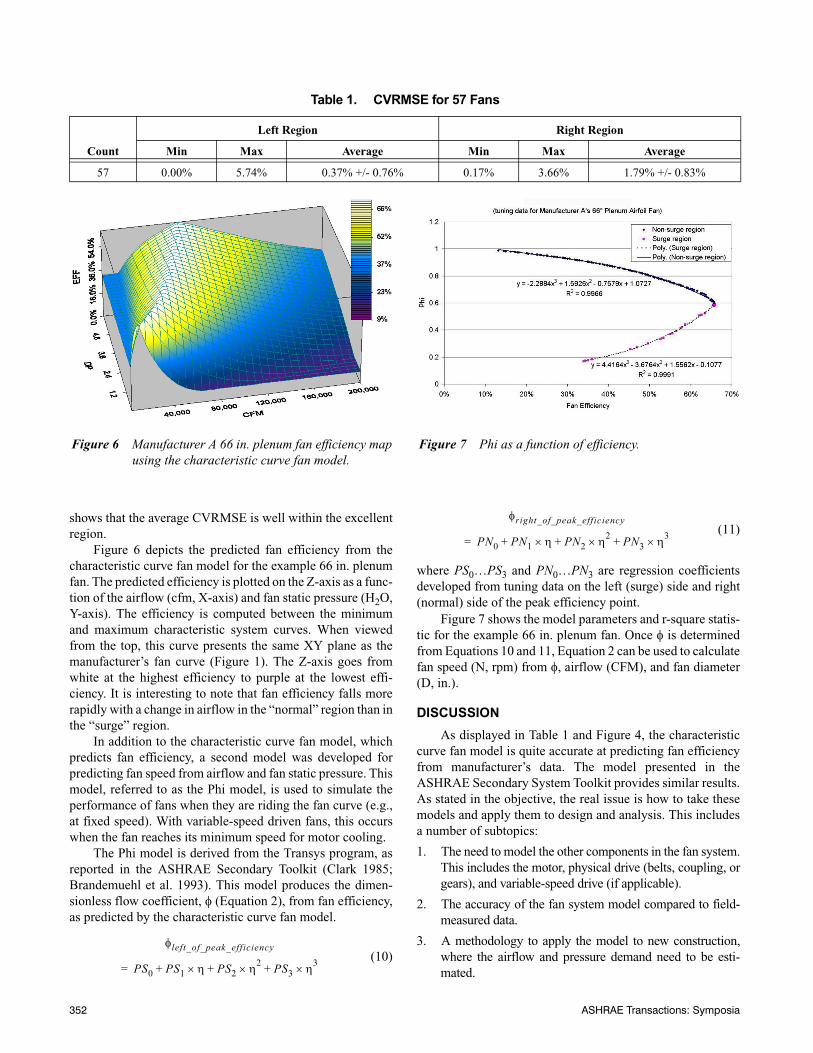
Figure 6 depicts the predicted fan efficiency from thecharacteristic curve fan model for the example 66 in. plenumfan. The predicted efficiency is plotted on the Z-axis as a func-tion of the airflow (cfm, X-axis) and fan static pressure (H2O,Y-axis). The efficiency is computed between the minimumand maximum characteristic system curves. When viewedfrom the top, this curve presents the same XY plane as themanufacturer’s fan curve (Figure 1). The Z-axis goes fromwhite at the highest efficiency to purple at the lowest effi-ciency. It is interesting to note that fan efficiency falls morerapidly with a change in airflow in the “normal” region than inthe “surge” region.

In addition to the characteristic curve fan model, whichpredicts fan efficiency, a second model was developed forpredicting fan speed from airflow and fan static pressure. Thismodel, referred to as the Phi model, is used to simulate theperformance of fans when they are riding the fan curve (e.g.,at fixed speed). With variable-speed driven fans, this occurswhen the fan reaches its minimum speed for motor cooling.

The Phi model is derived from the Transys program, asreported in the ASHRAE Secondary Toolkit (Clark 1985;Brandemuehl et al. 1993). This model produces the dimen-sionless flow coefficient, φ (Equation 2), from fan efficiency,as predicted by the characteristic curve fan model.

(10)

(11)

where PS0…PS3 and PN0…PN3 are regression coefficientsdeveloped from tuning data on the left (surge) side and right(normal) side of the peak efficiency point.

Figure 7 shows the model parameters and r-square statis-tic for the example 66 in. plenum fan. Once φ is determinedfrom Equations 10 and 11, Equation 2 can be used to calculatefan speed (N, rpm) from φ, airflow (CFM), and fan diameter(D, in.).

DISCUSSION

As displayed in Table 1 and Figure 4, the characteristiccurve fan model is quite accurate at predicting fan efficiencyfrom manufacturer’s data. The model presented in theASHRAE Secondary System Toolkit provides similar results.As stated in the objective, the real issue is how to take thesemodels and apply them to design and analysis. This includesa number of subtopics:

1. The need to model the other components in the fan system.This includes the motor, physical drive (belts, coupling, orgears), and variable-speed drive (if applicable).

2. The accuracy of the fan system model compared to field-measured data.

3. A methodology to apply the model to new construction,where the airflow and pressure demand need to be esti-mated.

Table 1. CVRMSE for 57 Fans

Count

Left Region Right Region

Min Max Average Min Max Average

57 0.00% 5.74% 0.37% +/- 0.76% 0.17% 3.66% 1.79% +/- 0.83%

Figure 6 Manufacturer A 66 in. plenum fan efficiency mapusing the characteristic curve fan model.

φleft_of_peak_efficiency

PS0 PS1+ η× PS2+ η2

× PS3+ η3

×=

φright_of_peak_efficiency

PN0 PN1+ η× PN2+ η2

× PN3+ η3

×=

Figure 7 Phi as a function of efficiency.


Both the characteristic curve fan model and the ASHRAESecondary Toolkit fan model produce fan efficiency as a func-tion of operating parameters. However, total fan energy is typi-cally more important for design studies. Fan energy cannot bedetermined without component models for motors, belts, andvariable-speed drives. The researchers have developed thesecomponent models and have assembled them into a fan systemmodel. This is documented in the project reports and will bethe subject of another ASHRAE paper. Resources for existingcomponent models include the following:

1. The research project web site, at <http://www.newbuild-ings.org/pier/index.html>; click on link for Large HVACIntegration.

2. The Department of Energy’s Motor Challenge markettransformation program (<http://www.oit.doe.gov/best-practices/motors/>) and MotorMaster+ Program (<http://mm3.energy.wsu.edu/mmplus/default.stm>) for modelsand performance data of poly phase motors.

3. Data on variable-speed drive efficiencies are reported inGao et al. (2001).

4. AMCA Publication 203-90 (AMCA 1990) for belt drives.

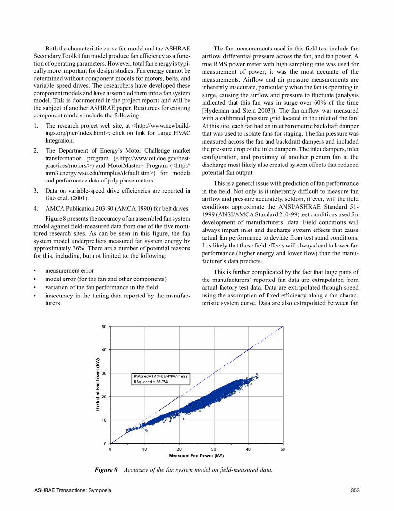
Figure 8 presents the accuracy of an assembled fan systemmodel against field-measured data from one of the five moni-tored research sites. As can be seen in this figure, the fansystem model underpredicts measured fan system energy byapproximately 36%. There are a number of potential reasonsfor this, including, but not limited to, the following:

• measurement error• model error (for the fan and other components)• variation of the fan performance in the field• inaccuracy in the tuning data reported by the manufac-

turers

The fan measurements used in this field test include fanairflow, differential pressure across the fan, and fan power. Atrue RMS power meter with high sampling rate was used formeasurement of power; it was the most accurate of themeasurements. Airflow and air pressure measurements areinherently inaccurate, particularly when the fan is operating insurge, causing the airflow and pressure to fluctuate (analysisindicated that this fan was in surge over 60% of the time[Hydeman and Stein 2003]). The fan airflow was measuredwith a calibrated pressure grid located in the inlet of the fan.At this site, each fan had an inlet barometric backdraft damperthat was used to isolate fans for staging. The fan pressure wasmeasured across the fan and backdraft dampers and includedthe pressure drop of the inlet dampers. The inlet dampers, inletconfiguration, and proximity of another plenum fan at thedischarge most likely also created system effects that reducedpotential fan output.

This is a general issue with prediction of fan performancein the field. Not only is it inherently difficult to measure fanairflow and pressure accurately, seldom, if ever, will the fieldconditions approximate the ANSI/ASHRAE Standard 51-1999 (ANSI/AMCA Standard 210-99) test conditions used fordevelopment of manufacturers’ data. Field conditions willalways impart inlet and discharge system effects that causeactual fan performance to deviate from test stand conditions.It is likely that these field effects will always lead to lower fanperformance (higher energy and lower flow) than the manu-facturer’s data predicts.

This is further complicated by the fact that large parts ofthe manufacturers’ reported fan data are extrapolated fromactual factory test data. Data are extrapolated through speedusing the assumption of fixed efficiency along a fan charac-teristic system curve. Data are also extrapolated between fan

Figure 8 Accuracy of the fan system model on field-measured data.


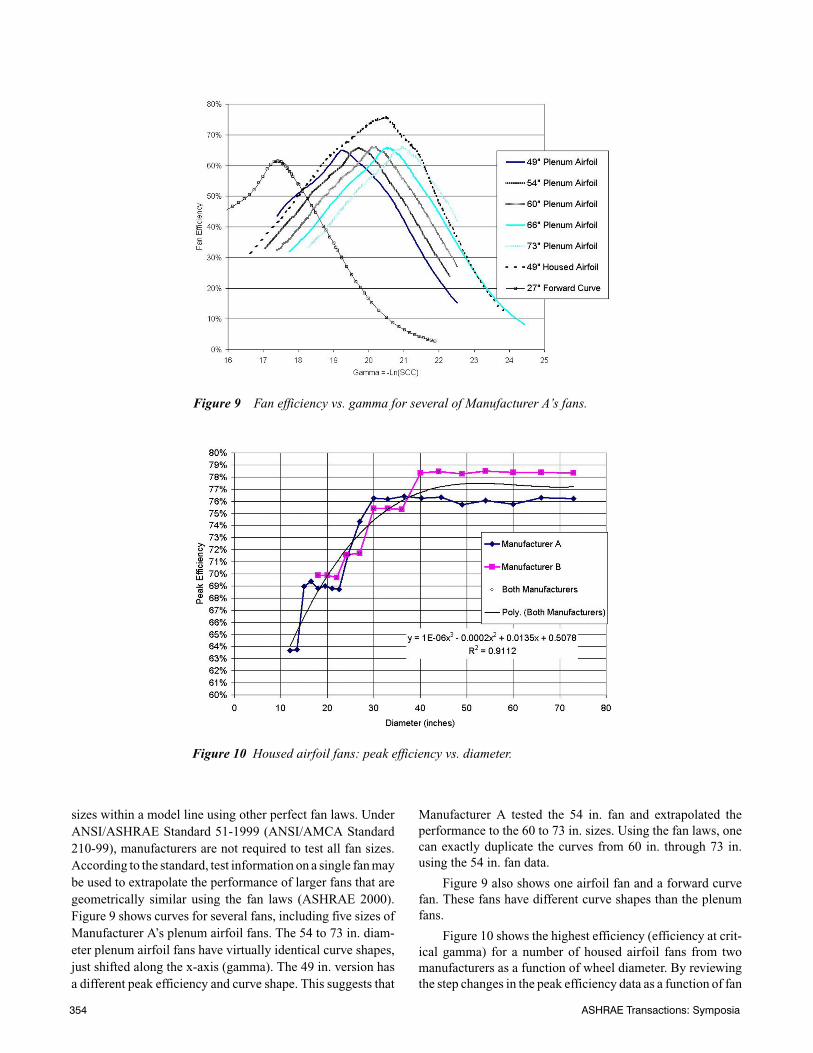
sizes within a model line using other perfect fan laws. UnderANSI/ASHRAE Standard 51-1999 (ANSI/AMCA Standard210-99), manufacturers are not required to test all fan sizes.According to the standard, test information on a single fan maybe used to extrapolate the performance of larger fans that aregeometrically similar using the fan laws (ASHRAE 2000).Figure 9 shows curves for several fans, including five sizes ofManufacturer A’s plenum airfoil fans. The 54 to 73 in. diam-eter plenum airfoil fans have virtually identical curve shapes,just shifted along the x-axis (gamma). The 49 in. version hasa different peak efficiency and curve shape. This suggests that

Manufacturer A tested the 54 in. fan and extrapolated theperformance to the 60 to 73 in. sizes. Using the fan laws, onecan exactly duplicate the curves from 60 in. through 73 in.using the 54 in. fan data.

Figure 9 also shows one airfoil fan and a forward curvefan. These fans have different curve shapes than the plenumfans.

Figure 10 shows the highest efficiency (efficiency at crit-ical gamma) for a number of housed airfoil fans from twomanufacturers as a function of wheel diameter. By reviewingthe step changes in the peak efficiency data as a function of fan

Figure 9 Fan efficiency vs. gamma for several of Manufacturer A’s fans.

Figure 10 Housed airfoil fans: peak efficiency vs. diameter.


diameter, it is clear from this figure which fans the manufac-turers tested and which they extrapolated. For example, bothManufacturer A and Manufacturer B tested their 30 in. fans.Manufacturer A then extrapolated the 30 in. data all the wayup to 73 in. (the variability in the peak efficiency of the Manu-facturer A 30 in. to 73 in. fans is due to rounding and samplingerror). Manufacturer B only extrapolated the 30 in. up to 36 in.,then they tested the 40 in.and extrapolated that all the way to73 in. Manufacturer A’s 30 in. is more efficient than Manufac-turer B’s 30 in. but not more efficient than the ManufacturerB’s 40 in. Had Manufacturer A tested a 40 in. (or larger) fan,they might have found that it had higher efficiency thanequally sized Manufacturer B’s fans.

To use the characteristic curve fan model in a designcontext, we suggest the following process:

1. Develop a simulation model of the facility.

2. Export the hourly demand for fan airflow cfm.

3. Bin the data by hours spent at increments of airflow (10 to20 bins should suffice).

4. Develop a system curve that represents the coincident pres-sure at each fan airflow. Note: this may actually be a familyof curves representing issues such as supply pressure resetcontrol and the fixed pressure overhead for individual fansrun alone or in parallel.

5. Evaluate the performance of alternate fans across the bindata using the system curves to develop a coincident pres-sure.

This, of course, is moot if software developers incorpo-rate the characteristic curve fan model in their programsdirectly for a parametric analysis.

CONCLUSIONS

As shown in this paper, it is possible to accurately predictmanufacturers’ fan performance using the characteristic curvefan model. However, it is a challenge to predict field perfor-mance due primarily to inaccuracies in instrumentation,system effects due to field conditions, and inaccuracies in themanufacturers’ reported performance data (due mostly fromtheir extrapolation of test data). From a design perspective,some of these issues are moot, as biases in instrumentation,measurement, and data reporting will tend to cancel out in acomparative analysis of design alternatives.

To serve as a design tool, a predictive fan model should bedeveloped to predict brake horsepower from airflow and fanstatic pressure. These are the inputs that are typically providedin a simulation tool. The model should also have discretesubmodels for the separate fan system components so thatanalysis can be done on the impact of design alternates foreach of those components.

Overall, the characteristic curve fan model meets all ofthese requirements. It is accurate at predicting manufacturers’data, relatively easy to tune, and could easily be incorporatedinto existing simulation tools. The authors have successfullyemployed it in Visual Basic code. There are limitations; this

model works for systems with fixed-speed fans and fans withvariable-speed drives, but it will not work for fans with inletvanes or variable-pitch blades. Those challenges are left up tofuture researchers.

Also left to future researchers is the development ofgeneralized fan models based on the characteristic curve fanmodel. The techniques described thus far require tuning dataspecific to each fan to be evaluated. However, there are clearpatterns between gamma curves for fans of the same type (seeFigure 9) A single gamma curve could be used to represent allfans of a certain type (housed airfoil, plenum airfoil, plenumflat blade, etc.). This curve could then be translated along thegamma axis using the perfect fan laws and along the efficiencyaxis as a function of diameter. Figure 10 shows such a functionfor housed airfoil fans.

ACKNOWLEDGMENTS

The authors would like to acknowledge the input andwork of other members of our research team, including CathyHiggins of the New Buildings Institute, Steve Taylor of TaylorEngineering, Erik Kolderup and Tianzhen Hong of Eley Asso-ciates, Lynn Qualman from SBW Consulting, Inc., and RogerLippman from New Horizon Technologies. They would alsolike to recognize the contributions of our technical advisoryteam members. Finally, special thanks to the numerous build-ing engineers and property managers at these sites for puttingup with our intrusions at their buildings and for their signifi-cant assistance in our work.

REFERENCES

AMCA. 1990. AMCA Publication 203-90, Field perfor-mance measurement of fan systems, 0203X90A-S.Arlington Heights, Ill.: The Air Movement and ControlAssociation International, Inc.

ASHRAE. 1999. ANSI/ASHRAE Standard 51-1999 (ANSI/AMCA Standard 210-99), Laboratory Methods of Test-ing Fans for Aerodynamic Performance Rating. Atlanta:American Society of Heating, Refrigerating and Air-Conditioning Engineers, Inc.

ASHRAE. 2000. 2000 ASHRAE Handbook—HVAC Systemsand Equipment, Chapter 18, Fans. Atlanta: AmericanSociety of Heating, Refrigerating and Air-ConditioningEngineers, Inc.

Brandemuehl, M.J., S. Gabel, and I. Andresen. 1993. HVAC2 Toolkit: Algorithms and Subroutines for SecondaryHVAC System Energy Calculations. Atlanta: AmericanSociety of Heating, Refrigerating and Air-ConditioningEngineers, Inc.

CALMAC. 2003. Data from the non-residential new-con-struction database available from the California Mea-surement Advisory Council’s web site, <http://www.calmac.org/>.

Clark, D.R. 1985. HVACSIM+ building systems and equip-ment simulation program: Reference Manual. NBSIR


84-2996, U.S. Department of Commerce, WashingtonD.C.

DOE (Department of Energy). 1980. DOE 2 Reference Man-ual, Part 1, Version 2.1. Lawrence Berkeley NationalLaboratories, Berkeley Calif., May.

Gao, X., S.A. McInerny, and S.P. Kavanaugh. 2001. Efficien-cies of an 11.2 kW variable speed motor and drive.ASHRAE Transactions 107(2). Atlanta: American Soci-ety of Heating, Refrigerating and Air-ConditioningEngineers, Inc.

Hydeman, M., J. Stein. 2003. A fresh look at fan selectionand control. HPAC Magazine, May.

Kolderup, E., M. Hydeman, M. Baker, and R.L. Qualmann.2002. Measured performance and design guidelines forlarge commercial HVAC systems. ACEEE Conferenceon Energy Efficiency, August.

DISCUSSION

David Yuill, Principal, Building Solutions Inc., Omaha,Neb.: We have done some similar work in which we devel-oped a model to predict airflow through a fan using the designfan curve, fan head, and fan speed as inputs. We set up an

experiment to test this model, but we found that the manufac-turer’s fan curves were not accurate. Have you found this, andare you aware of any data on fan curve accuracy?

Jeff Stein: As noted in the paper we did not find a good corre-lation between measured fan energy and predicted energy(based on manufacturer's data). There are many possiblereasons including: (1) The pressure and air flow sensors usedin the field tests may be inaccurate. (2) Even if the sensors areaccurate, field tests of fan operating static cannot match theAMCA test conditions of "fan static" in the lab: it is impossi-ble to measure "fan static" (the Y axis on a fan curve) in thefield since the installation conditions are completely different.System effects play havoc with fan performance in the field.(3) Manufacturer's do not test all sizes. The AMCA ratingstandard for fans allows them to test a fan and extrapolate theresults to all larger fans of the same type. (4) Accuracy of themanufacturer's tests. We noticed that performance data forsome fan types got worse and then better as you move to largersizes. This suggests that there may be variability in the manu-facturing or testing processes. We are not aware of any data onfan curve accuracy.

fan surging

Documents