faraday discussions - university of california, berkeley · 488 | faraday discuss., 2013, 167,...

Faraday DiscussionsCite this: Faraday Discuss., 2013, 167, 485

PAPER

Publ

ishe

d on

30

May

201

3. D

ownl

oade

d by

Pri

ncet

on U

nive

rsity

on

01/1

0/20

14 0

3:16

:15.

View Article OnlineView Journal | View Issue

Corresponding states for mesostructure anddynamics of supercooled water

David T. Limmer and David Chandler*

Received 6th May 2013, Accepted 30th May 2013

DOI: 10.1039/c3fd00076a

Water famously expands upon freezing, foreshadowed by a negative coefficient of

expansion of the liquid at temperatures close to its freezing temperature. These

behaviors, and many others, reflect the energetic preference for local tetrahedral

arrangements of water molecules and entropic effects that oppose it. Here, we provide

theoretical analysis of mesoscopic implications of this competition, both equilibrium

and non-equilibrium, including mediation by interfaces. With general scaling

arguments bolstered by simulation results, and with reduced units that elucidate

corresponding states, we derive a phase diagram for bulk and confined water and

water-like materials. For water itself, the corresponding states cover the temperature

range of 150 K to 300 K and the pressure range of 1 bar to 2 kbar. In this regime, there

are two reversible condensed phases – ice and liquid. Out of equilibrium, there is

irreversible polyamorphism, i.e., more than one glass phase, reflecting dynamical arrest

of coarsening ice. Temperature–time plots are derived to characterize time scales of the

different phases and explain contrasting dynamical behaviors of different water-like

systems.

1 Introduction

Supercooled liquids exist in a metastable equilibrium made possible by a sepa-ration of timescales between local liquid equilibration and global crystallization.1

Supercooled water is no different in this regard. However, the magnitude of theseparation of timescales in supercooled water is of particular relevance due tospeculation regarding the behavior of the thermodynamic properties of liquidwater at very low temperatures.2 In this work, we describe a theory for corre-sponding states that relates the low temperature, low pressure phase diagramwith the time–temperature–transformation diagram for supercooled water andwater-like systems. Our derivations use scaling theories with assumptions testedagainst molecular simulation. The relationships elucidate the connectionsbetween behaviors found for different molecular simulation models of water andfor different water-like substances.

Department of Chemistry, University of California, Berkeley, California, 94702, USA. E-mail: chandler@

berkeley.edu

This journal is ª The Royal Society of Chemistry 2013 Faraday Discuss., 2013, 167, 485–498 | 485

http://dx.doi.org/10.1039/c3fd00076a

http://pubs.rsc.org/en/journals/journal/FD

http://pubs.rsc.org/en/journals/journal/FD?issueid=FD013167

Faraday Discussions PaperPu

blis

hed

on 3

0 M

ay 2

013.

Dow

nloa

ded

by P

rinc

eton

Uni

vers

ity o

n 01

/10/

2014

03:

16:1

5.

View Article Online

Fig. 1 shows the portion of the phase diagram for supercooled water relevant tothis paper. Temperature, T, ranges from ambient conditions to deep into thesupercooled regime, and pressure, p, ranges from atmospheric conditionsthrough the range of stability for ordinary hexagonal ice. Experimentally, thisregion corresponds to 150 K < T < 300 K and 0 kbar < p < 2 kbar.14 The locations ofspecic features relative to experiment vary from one molecular model toanother.15 This variability reects a delicate competition between entropy andenergy that is intrinsic to any reasonable model of water or water-like system.

One manifestation of this competition is the existence of the temperature ofmaximumdensity. We use Tmax to denote the value of this temperature at ambient(i.e., low pressure) conditions. For experimental water, Tmax z 277 K. The energy–entropy balance manifested in the density maximum is shied to lower temper-atures as elevated pressures favor denser packing. A measure of this shi isprovided by the slope of the melting line or in terms of a reference pressure po ¼�DH/10 DV, where DH and DV are, respectively, the enthalpy and volume changesupon melting. For experimental water, po z 3.7 kbar. We use Tmax and po tocompare the properties of different water models as well as to enable comparisonwith experiment.3–7,7,14,16 Thus, the phase diagram in Fig. 1 employs the reducedvariables

~p ¼ p/po and ~T ¼ T/Tmax. (1)

In this way, Fig. 1 relates results from various models and experiments for theonset temperature, To, and the homogeneous nucleation temperature, Ts. Theformer, To, marks the crossover to correlated (i.e., hierarchical) dynamics,17 and itplays a central role in formulas for the temperature dependence of liquid relax-ation rates, as discussed below. The latter, Ts, marks the crossover to liquidinstability,18–20 and it plays a central role in the temperature dependence of ice

Fig. 1 The ~p–~T phase diagram for supercooled water. These symbols refer to the pressure, p, and thetemperature T, in units of the reference pressure, po, and the reference temperature, Tmax, for eachspecific material,3–7 see text. The lines refer to theoretically expected trends as functions of pressure forthe dynamical onset temperature, To, for the liquid limit of stability temperature, Ts, and for a glasstransition temperature, Tg. Symbols indicate locations of these temperatures in the reduced units asobtained from experiment and from different molecular simulation models, where the key employsstandard acronyms for each system.8–13 For the glass transition, the line marks the stage where the liquidreorganization time exceeds 1014 so, where the reference time, so, is that reorganization time at theonset to correlated dynamics (so z 1 ps for liquid water).

486 | Faraday Discuss., 2013, 167, 485–498 This journal is ª The Royal Society of Chemistry 2013


Paper Faraday DiscussionsPu

blis

hed

on 3

0 M

ay 2

013.

Dow

nloa

ded

by P

rinc

eton

Uni

vers

ity o

n 01

/10/

2014

03:

16:1

5.

View Article Online

coarsening, also as discussed below. These temperatures are material properties.Fig. 1 also shows a reduced glass transition temperature, ~Tg ¼ Tg/Tmax. Thistemperature is dened as that where the reversible structural relaxation time ofliquid water equals 100 s.

Glass phases of water, where aging occurs on time scales of 100 s or longer, arenot generally accessible by straightforward supercooling because bulk liquidwater spontaneously freezes into crystal ice at temperatures below Ts ¼ Ts(p).Freezing in this regime occurs on milli-second or shorter time scales.21 Anamorphous solid can be reached with a cooling trajectory that is initially fastenough to arrest crystallization, and nally cold enough to produce very slowaging. Alternatively, an amorphous solid can be reached by cooling while per-turbing water with surfaces that inhibit crystallization. A glass transitiontemperature of water is therefore not a material property because its valuedepends upon the protocol by which the material is driven out of equilibrium.Surface mediated approaches to amorphous solids can yield Tg's that are higherthan those produced by rapid temperature quenches. The Tg graphed in Fig. 1 isnecessarily an upper bound to those glass transition temperatures.

Dynamics in the vicinity of Ts(p) exhibits a two-step coarsening of the crystalphase.20,22,23 First, disperse nano-scale domains of local crystal order formthroughout the melt; second, on a much longer time scale, the nano-scaledomains meld into much larger ordered domains. These steps are arrested whenforming glass.24 Congurations appearing at the initial stages of this coarseningare oen observed in computer simulations of water. These congurations aretransient states that are almost as oen confused with the presence of two distinctsupercooled liquid phases.† There is one exceptional case, a water-like modelwhere transient states have not yet been observed. Specically, Giovambattistaand co-workers25 suggest that the SPC/E model does not exhibit this phenom-enon. In that particular case, we shall see, it seems that the transient states havebeen overlooked simply because the relevant part of the phase diagram near Ts(p)has been overlooked.

Two distinct reversible liquids in coexistence would imply the existence of asecond critical point of the sort suggested by Stanley and his co-workers.26 Notsurprisingly, all reports of a low-temperature critical point in water or water-likesystems locate a point on or near Ts(p). In fact, all the simulation points clusteredaround that line in Fig. 1 have been incorrectly identied as low-temperaturecritical points.8–13 Similarly, in experimental work, Mishima locates a putativecritical point27 close to the experimental limit of liquid stability.28 We haveanalyzed and disproved this notion of a liquid–liquid transition for severaldifferent computer simulation models of water and water-like systems.20

We mention the disproved notion only to emphasize that the equilibriumphase diagram by itself gives an incomplete picture of the behavior of super-cooled water. Supercooled water, being a metastable state, behaves reversibly foronly nite observation times. The specic length of that time depends on theseparation of timescales between local equilibration of liquid congurations andglobal crystallization. When the gap between these timescales is no longer large

† The list of representative papers is long. We have provided a summary elsewhere.20



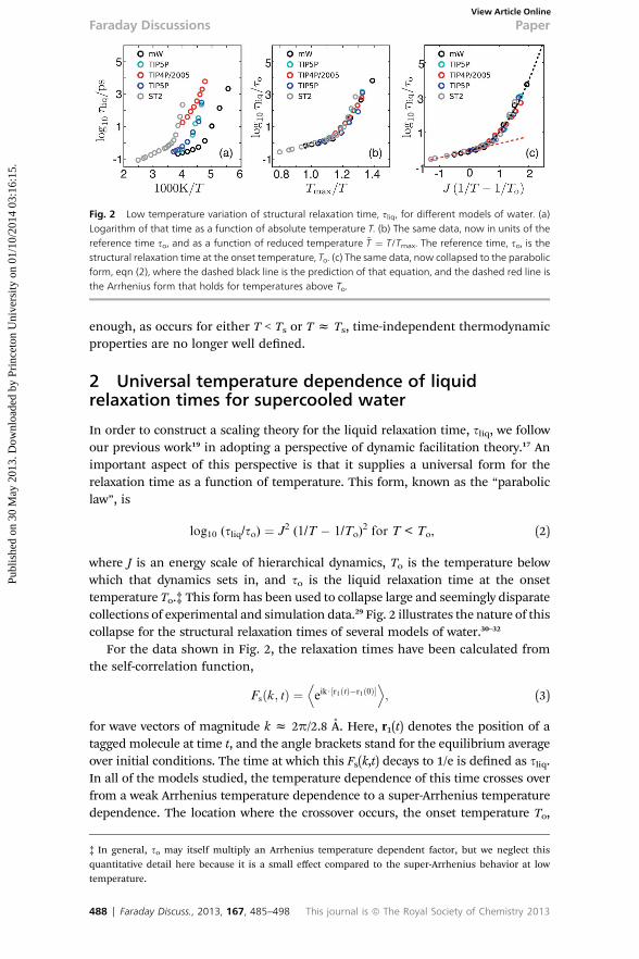
Fig. 2 Low temperature variation of structural relaxation time, sliq, for different models of water. (a)Logarithm of that time as a function of absolute temperature T. (b) The same data, now in units of thereference time so, and as a function of reduced temperature ~T ¼ T/Tmax. The reference time, so, is thestructural relaxation time at the onset temperature, To. (c) The same data, now collapsed to the parabolicform, eqn (2), where the dashed black line is the prediction of that equation, and the dashed red line isthe Arrhenius form that holds for temperatures above To.


blis

hed

on 3

0 M

ay 2

013.

Dow

nloa

ded

by P

rinc

eton

Uni

vers

ity o

n 01

/10/

2014

03:

16:1

5.

View Article Online

enough, as occurs for either T < Ts or T z Ts, time-independent thermodynamicproperties are no longer well dened.

2 Universal temperature dependence of liquidrelaxation times for supercooled water

In order to construct a scaling theory for the liquid relaxation time, sliq, we followour previous work19 in adopting a perspective of dynamic facilitation theory.17 Animportant aspect of this perspective is that it supplies a universal form for therelaxation time as a function of temperature. This form, known as the “paraboliclaw”, is

log10 (sliq/so) ¼ J2 (1/T � 1/To)2 for T < To, (2)

where J is an energy scale of hierarchical dynamics, To is the temperature belowwhich that dynamics sets in, and so is the liquid relaxation time at the onsettemperature To.‡ This form has been used to collapse large and seemingly disparatecollections of experimental and simulation data.29 Fig. 2 illustrates the nature of thiscollapse for the structural relaxation times of several models of water.30–32

For the data shown in Fig. 2, the relaxation times have been calculated fromthe self-correlation function,

Fsðk; tÞ ¼Deik$½r1ðtÞ�r1ð0Þ�

E; (3)

for wave vectors of magnitude k z 2p/2.8 A. Here, r1(t) denotes the position of atagged molecule at time t, and the angle brackets stand for the equilibrium averageover initial conditions. The time at which this Fs(k,t) decays to 1/e is dened as sliq.In all of the models studied, the temperature dependence of this time crosses overfrom a weak Arrhenius temperature dependence to a super-Arrhenius temperaturedependence. The location where the crossover occurs, the onset temperature To,

‡ In general, so may itself multiply an Arrhenius temperature dependent factor, but we neglect thisquantitative detail here because it is a small effect compared to the super-Arrhenius behavior at lowtemperature.




blis

hed

on 3

0 M

ay 2

013.

Dow

nloa

ded

by P

rinc

eton

Uni

vers

ity o

n 01

/10/

2014

03:

16:1

5.

View Article Online

varies from model to model as does the reference timescale so. This variability inpart reects quantitative differences between phase diagrams for each of themodels. Indeed, Fig. 2b shows that the temperature dependence of the relaxationtimes can be collapsed by referencing the data to the temperature of maximumdensity. It is a remarkable result given the wide variation of Tmax, ranging from250 K to 320 K for the different models.5

In addition, Fig. 2c shows that the relaxation time data also collapses whenreferenced to the onset temperature, To, and that the collapsed data obeys theparabolic law for all T < To. This nding establishes that

To z Tmax. (4)

Further, collapsing data to the parabolic law reveals that J/To varies betweenmodels of water by no more that 5% and on average by only 1%. This typical value isJ/To z 7.4. For the models considered here, so varies between 0.3 ps and 8.0 ps, andthis variability largely reects the density differences betweenmodels at low pressure.

The collapse of the relaxation times for the difference models as a function ofTmax implies a universality in the behavior of the glass transition for these modelsand, by proxy, for experiment. As we have done previously,19 we can dene a locusof laboratory glass transitions as the locations in the phase diagram where theliquid relaxation time is equal to 1014 so, which for many of the models impliessliq(Tg) z 100 s, so that with eqn (2) we have,

Tg=Toz� ffiffiffiffiffi

14p

To=J þ 1��1

: (5)

Taking J/To z 7.4 and To z Tmax, we therefore conclude that for water andwater-like models, Tg z 0.62Tmax. This value yields the glass-transition linegraphed in Fig. 1, where the slope of the line is the same as that for To(p).Experimentally, the density maximum for water occurs at Tmax z 277, thereforeour predicted glass transition is Tg z 172 K. This temperature agrees with ourprevious work inferring the glass transition temperature from relaxation data ofconned water.19 It also provides an upper bound to values for Tg obtained withother experimental protocols.33,34

3 Molecular theory for J, so and To

The energy, time and temperature parameters in eqn (2) can be computed frommicroscopic theory following the procedures of Keys et al.35 The procedures arebased upon mapping the dynamics of atomic degrees of freedom to dynamics of akinetically constrained East model.36 The parabolic law, eqn (2), is a consequence ofthat mapping.

To illustrate the procedure for water, we have carried out molecular dynamicssimulations of equilibrated water models to determine the net number ofenduring displacements of length a appearing in N-molecule trajectories that runfor observation times tobs. This number of displacements is

Ca ¼XNi¼1

Xtobs=Dtj¼0

Q�jrið jDtþ DtÞ � rið jDtÞj � a

�(6)



Fig. 3 Excitation concentration for the mW model at ambient pressure for enduring displacementlengthscales, a, between 1.5 and 3.5 A. The dashed line has unit slope illustrating the Boltzmann scaling,eqn (8). The inset shows the logarithmic scaling of Ja with a. The dashed line is a fit to the data for eqn (9)with g ¼ 0.625.


blis

hed

on 3

0 M

ay 2

013.

Dow

nloa

ded

by P

rinc

eton

Uni

vers

ity o

n 01

/10/

2014

03:

16:1

5.

View Article Online

where Q(x) is 1 for x > 0 and zero otherwise, Dt is the mean instanton time forenduring displacements of length a, and �ri(t) is the position of particle iaveraged over the time interval t � dt/2 to t + dt/2. The averaging over dtcoarse-grains out irrelevant vibrational motions. The instanton time, Dt, istaken to be large enough that non-enduring transitions are also removedfrom consideration. The two times, Dt > dt, are determined as prescribed byKeys et al.35

The meanmobility (or excitation concentration) is the net number of enduringtransitions per molecule per unit time, i.e.,

ca ¼ hCai/(Ntobs/Dt). (7)

Its dependence upon temperature and displacement length is illustrated in Fig. 3.According to facilitation theory, ca should have a Boltzmann temperaturedependence, with an energy scale that grows logarithmically with displacementlength. That is,

ca f exp[�Ja(1/T � 1/To)] for T < To, (8)

and

Ja0 ¼ Ja � g Js ln(a0/a), (9)

where s is a reference molecular length and g is a system-dependent constant.§The data graphed in Fig. 3 shows that for the model considered, the mWmodel ofwater, the theoretical expectations are obeyed. We have adopted the referencelength s¼ 2.5 A, which is close to the diameter of the molecule in the mWmodel,and nd g ¼ 0.625, To ¼ 244 K z Tmax ¼ 250 K, and Js/To ¼ 23.

§ Keys et al.35 use the symbol g for what we call g. We use g to refer to the surface tension.




blis

hed

on 3

0 M

ay 2

013.

Dow

nloa

ded

by P

rinc

eton

Uni

vers

ity o

n 01

/10/

2014

03:

16:1

5.

View Article Online

According to facilitation theory,35 eqn (8) and (9) imply

ln(sliq/so) ¼ (J2sg/df)(1/T � 1/To)2 for T < To, (10)

where df is the fractal dimension of dynamic heterogeneity, which for d ¼ 3 isabout 2.6. Eqn (10) therefore yields

J ¼ Jsffiffiffiffiffiffiffiffiffiffiffiffiffiffiffiffiffig=2:3 df

p(11)

where the factor of 2.3 in the square-root accounts for the conversion betweenbase e and base 10 logarithms.{ Applying eqn (11) with the computed parametersyields J/To ¼ 7.4, in good agreement with the empirical value for this ratioreported in the previous section. The empirical value was obtained from ttingdata for various water models. Here, we have succeeded at deriving this valuefrom a molecular calculation.

4 Theory for crystallization time

To estimate the timescale for crystallization, sxtl, we start with the usualexpression,

sxtl ¼ n�1eDF/T (12)

where DF is the free energy cost for growing a nascent crystal and n�1 is thetimescale for adding material to the burgeoning phase. Typical forms for DF canbe motivated by classical nucleation theory, which has been shown previously toyield accurate results for nucleation rate of models of water at moderate super-cooling.37 In general, this free energy can be written as

DF/T ¼ F(g/Dh)(T/Tm � 1)�2, (13)

where g is surface tension for liquid–crystal coexistence, andF(g/Dh) is a functionof the ratio of g to the difference of enthalpy density between those phases. Theratio is approximately temperature independent.1,19 The temperature-dependentfactor, (T/Tm � 1)�2, comes from expanding the chemical potential difference tolowest non-trivial order in T � Tm.

The timescale for adding material to a growing cluster, n�1, is expected to beapproximately athermal for T > To, but to become signicantly temperaturedependent below that onset temperature. In particular, we expect n�1 f D, whereD is the molecular self-diffusion constant, and below the onset temperature,supercooled liquids generically obey a fractional Stokes–Einstein relationship,38

D f s�zliq . (14)

For T > To, z ¼ 1.39 On the other hand, for T < To, z z 3/4.38 This value for theexponent is predicted by the East model.40 Adopting a fractional Stokes–Einsteinrelation with eqn (2) implies a super-Arrhenius form for n�1,

{ Keys et al.35 employ natural logarithms in their use of the parabolic law, and thus the factor of 2.3 doesnot appear in their equations.



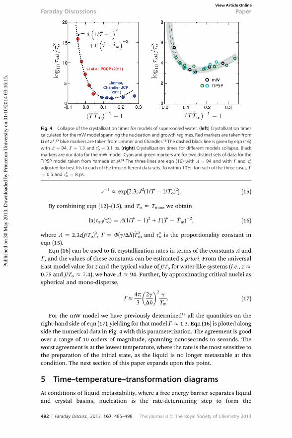
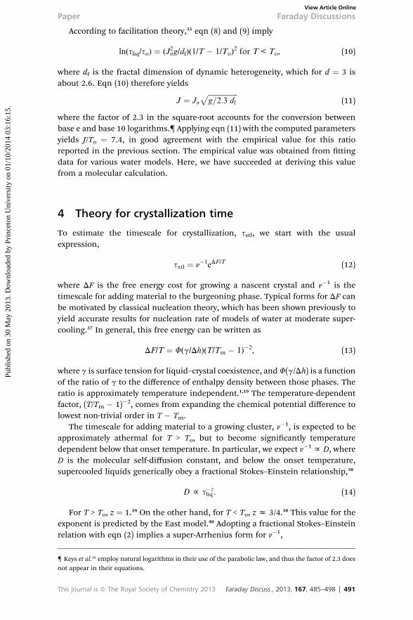
Fig. 4 Collapse of the crystallization times for models of supercooled water. (left) Crystallization timescalculated for the mWmodel spanning the nucleation and growth regimes. Red markers are taken fromLi et al.,37 blue markers are taken from Limmer and Chandler.18 The dashed black line is given by eqn (16)with L ¼ 94, G ¼ 1.3 and sxo ¼ 0.1 ps. (right) Crystallization times for different models collapse. Blackmarkers are our data for the mWmodel. Cyan and green markers are for two distinct sets of data for theTIP5P model taken from Yamada et al.31 The three lines are eqn (16) with L ¼ 94 and with G and sxoadjusted for best fits to each of the three different data sets. To within 10%, for each of the three cases, Gz 0.5 and sxo z 8 ps.


blis

hed

on 3

0 M

ay 2

013.

Dow

nloa

ded

by P

rinc

eton

Uni

vers

ity o

n 01

/10/

2014

03:

16:1

5.

View Article Online

n�1 f exp[2.3zJ2(1/T � 1/To)2]. (15)

By combining eqn (12)–(15), and To z Tmax, we obtain

ln(sxtl/sxo) ¼ L(1/ ~T � 1)2 + G( ~T � ~Tm)

�2, (16)

where L ¼ 2.3z(J/To)2, G ¼ F(g/Dh)~T2

m and sxo is the proportionality constant ineqn (15).

Eqn (16) can be used to t crystallization rates in terms of the constants L andG, and the values of these constants can be estimated a priori. From the universalEast model value for z and the typical value of J/To for water-like systems (i.e., zz0.75 and J/To z 7.4), we have Lz 94. Further, by approximating critical nuclei asspherical and mono-disperse,

Gz4p

3

�2g

Dh

�2g

Tm

: (17)

For the mW model we have previously determined19 all the quantities on theright-hand side of eqn (17), yielding for thatmodelGz 1.3. Eqn (16) is plotted alongside the numerical data in Fig. 4 with this parameterization. The agreement is goodover a range of 10 orders of magnitude, spanning nanoseconds to seconds. Theworst agreement is at the lowest temperature, where the rate is the most sensitive tothe preparation of the initial state, as the liquid is no longer metastable at thiscondition. The next section of this paper expands upon this point.

5 Time–temperature–transformation diagrams

At conditions of liquid metastability, where a free energy barrier separates liquidand crystal basins, nucleation is the rate-determining step to form the




blis

hed

on 3

0 M

ay 2

013.

Dow

nloa

ded

by P

rinc

eton

Uni

vers

ity o

n 01

/10/

2014

03:

16:1

5.

View Article Online

equilibrium phase. Two data sets taken from the literature have used differentrare-event sampling techniques to compute these times for a range of tempera-tures for the mW model. Limmer and Chandler18 computed the nucleation rateconstant following a standard Bennett–Chandler procedure.41 Li et al.37 calculatedthe nucleation rate using forward-ux sampling42 with an order parameter basedon a crystalline cluster sizes. To the extent that the kinetics is nucleation limited,both calculations are expected to have the same temperature dependence.However, because each used different order parameters and basin denitions, theprefactors can be different. In order to compare both data sets, we determine theratio of prefactors by equating the rate at T ¼ 220 K, which was calculated in bothstudies. These data sets are shown in le panel of Fig. 4.

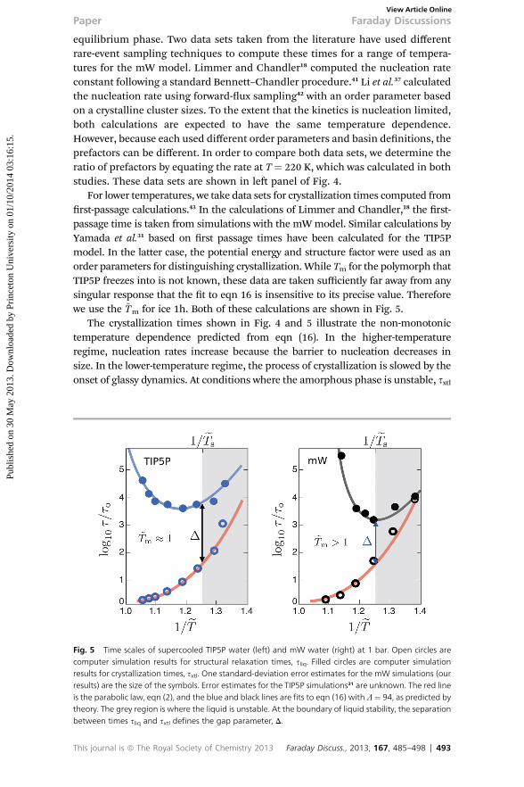
For lower temperatures, we take data sets for crystallization times computed fromrst-passage calculations.43 In the calculations of Limmer and Chandler,18 the rst-passage time is taken from simulations with the mWmodel. Similar calculations byYamada et al.31 based on rst passage times have been calculated for the TIP5Pmodel. In the latter case, the potential energy and structure factor were used as anorder parameters for distinguishing crystallization. While Tm for the polymorph thatTIP5P freezes into is not known, these data are taken sufficiently far away from anysingular response that the t to eqn 16 is insensitive to its precise value. Thereforewe use the ~Tm for ice 1h. Both of these calculations are shown in Fig. 5.

The crystallization times shown in Fig. 4 and 5 illustrate the non-monotonictemperature dependence predicted from eqn (16). In the higher-temperatureregime, nucleation rates increase because the barrier to nucleation decreases insize. In the lower-temperature regime, the process of crystallization is slowed by theonset of glassy dynamics. At conditions where the amorphous phase is unstable, sxtl

Fig. 5 Time scales of supercooled TIP5P water (left) and mW water (right) at 1 bar. Open circles arecomputer simulation results for structural relaxation times, sliq. Filled circles are computer simulationresults for crystallization times, sxtl. One standard-deviation error estimates for the mW simulations (ourresults) are the size of the symbols. Error estimates for the TIP5P simulations31 are unknown. The red lineis the parabolic law, eqn (2), and the blue and black lines are fits to eqn (16) with L¼ 94, as predicted bytheory. The grey region is where the liquid is unstable. At the boundary of liquid stability, the separationbetween times sliq and sxtl defines the gap parameter, D.



Table 1 Summary of properties for water and water models, with standard acronyms identifyingdifferent models.3–7,14,16,19 All properties are measured at ambient pressure, and ice properties refer to ice1h. See text for the meanings of symbols and the methods by which the properties are determined

Model Tmax/K po/kbar ~Tm ~To J/To so/ps sxo/ps G D

Experiment 277 3.7 0.99 0.98 7.4 1.0 0.3 1.2 3.4mW 250 10.0 1.09 0.98 7.0 0.6 0.1 1.3 1.6SW 1350 16.6 1.20 — — — — — —SPC/E 241 2.7 0.89 1.03 7.7 0.4 — — —ST2 320 3.4 0.94 0.95 7.6 3.0 — — 2.4TIP4P 253 3.7 0.92 — — — — — —TIP4P/2005 277 3.4 0.90 0.99 7.5 9.0 — — —TIP5P 285 19.4 0.96 0.98 7.6 0.2 8.0 0.5 2.1


blis

hed

on 3

0 M

ay 2

013.

Dow

nloa

ded

by P

rinc

eton

Uni

vers

ity o

n 01

/10/

2014

03:

16:1

5.

View Article Online

becomes limited by mass diffusion, which from eqn (14) is proportional to sliq. Inthis region of the phase diagram, the liquid state is no longer physically realizable.

In plotting sxtl in Fig. 4, we use a different reduced temperature scale thanprevious plots of sliq. The different scale is chosen to emphasize the crossoverregion, where nucleation and growth compete. This particular scale also allowsfor crystallization times to be collapsed for different models because, to rst orderin L/G, this scale locates the minimum in sxtl. The location is the solution to aquadratic polynomial found by equating the nucleation and growth terms.k Thisscaling holds only for T far below Tm. Away from the singular response at T ¼ Tm,this form is conserved from model to model as it reects the crossover touniversal structural relaxation times away from the nucleation dominated regime.

In Fig. 5 we show both sliq and sxtl to illustrate how the separation of timescalesevolves as a function of temperature for different models of water. By consideringtwo cases, where To z Tm and where To < Tm, we see large variation in the time-scale gap between liquid relaxation fastest crystallization. To quantify this vari-ation between models, we dene

D ¼ log10sxtlsliq

T¼Ts

; (18)

and subtract eqn (2) from 16 to predict how this gap parameter changes with ~Tm.For the mWmodel, the parameters in this equation predict Dz 1.6, in agreementwith simulation. For experimental water, ~Tm¼ 0.99, and G can be computed usingeqn (17) and known values for g and Dh, yielding G z 1.2.** As such, eqn (18)givesD¼ 3.4, consistent with cooling rates required to bypass crystal nucleation.21

The location of the minimum crystallization time for experiment can be similarlypredicted, and this yields ~T ¼ 0.77 or T z 215 K, which is close to, though lowerthan, previous estimates.22 One may also use this analysis to predict the timescales on which models of water will exhibit complex coarsening dynamicsresulting in articial polyamorphism.20

Table 1 summarizes material properties noted in this and preceding sections.Blanks (—) in the table refer to properties that have not yet been determined.Viewing the variability between models for the values for Tmax and po elucidates

k The solution for the minima is ~T ¼ (~Tm + u)/2 + [(u + ~Tm)2 � 4~Tm]

1/2/2, where u ¼ 1 � (L/G)1/2.

** Eisenberg and Kauzmann14 gives Dhz 3.0� 105 kJ m�3, and as we have done previously19 we take g tobe an average of the values presented in Granasy et al.44 or g ¼ 32 mJ m�2.




blis

hed

on 3

0 M

ay 2

013.

Dow

nloa

ded

by P

rinc

eton

Uni

vers

ity o

n 01

/10/

2014

03:

16:1

5.

View Article Online

how apparent different behaviors of different models can simply reect differentcorresponding states.

6 Mesostructured supercooled water

The lengthscale over which the arguments presented in the previous sections areapplicable to supercooled water reects the lengthscale over which orientationalorder is correlated. We have previously studied these correlations using thephenomenological Hamiltonian of the form,

H ½qðrÞ� ¼ðr

�f ½qðrÞ� þm

2jVqðrÞj2

�; (19)

where q(r) is an order parameter that measures the amount of local orientationalorder at a point r, f(q) is a free energy density,

f(q) ¼ a(T � Ts)q2/2 � wq3 + uq4, (20)

and a, w, u and m are positive constants determined by Dh, Tm and g.19 ThisHamiltonian is isomorphic with that of van der Waals for liquid–vapor coexis-tence.45 Consequently, mean proles for q(r) subject to external boundaryconditions yield smooth order-parameter proles like those at a liquid–vaporinterface. Instantaneously, this eld can be represented in a discrete basis andsampled with an interacting lattice gas.46 Such a coarse-grained representation isamenable to large-scale computations, beyond what are tractable with atomisticmodels.

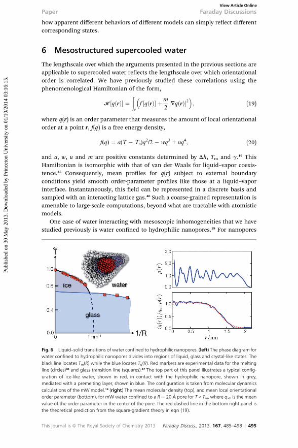
One case of water interacting with mesoscopic inhomogeneities that we havestudied previously is water conned to hydrophilic nanopores.19 For nanopores

Fig. 6 Liquid–solid transitions of water confined to hydrophilic nanopores. (left) The phase diagram forwater confined to hydrophilic nanopores divides into regions of liquid, glass and crystal-like states. Theblack line locates Tm(R) while the blue locates Tg(R). Red markers are experimental data for the meltingline (circles)48 and glass transition line (squares).47 The top part of this panel illustrates a typical config-uration of ice-like water, shown in red, in contact with the hydrophilic nanopore, shown in grey,mediated with a premelting layer, shown in blue. The configuration is taken from molecular dynamicscalculations of the mW model.19 (right) The mean molecular density (top), and mean local orientationalorder parameter (bottom), for mW water confined to a R ¼ 20 A pore for T < Tm, where qxtl is the meanvalue of the order parameter in the center of the pore. The red dashed line in the bottom right panel isthe theoretical prediction from the square-gradient theory in eqn (19).



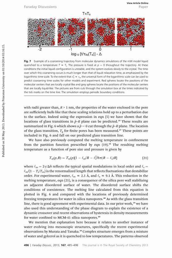
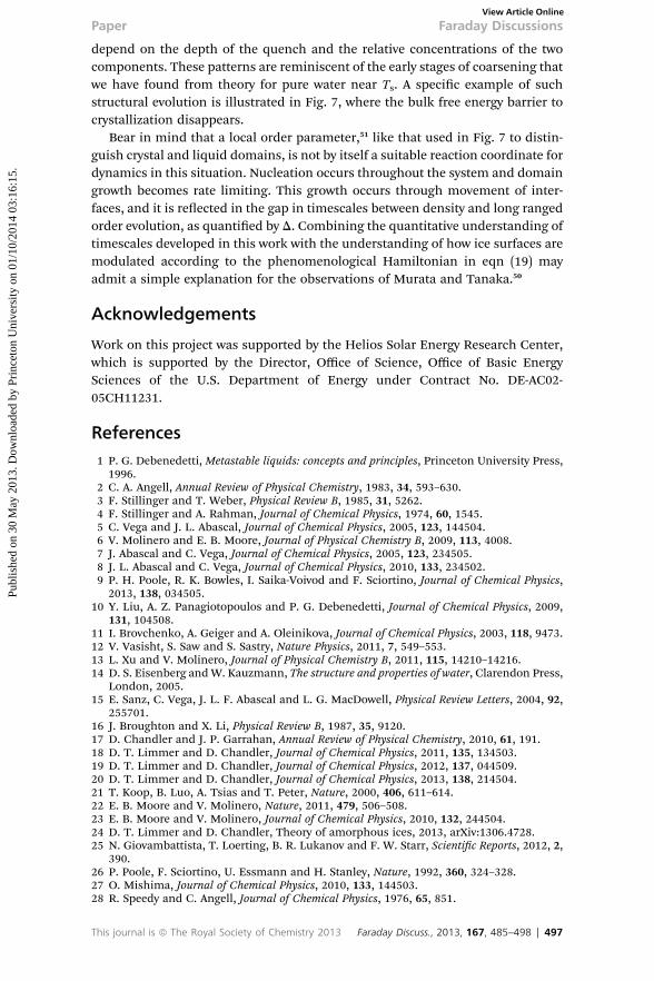
Fig. 7 Example of a coarsening trajectory from molecular dynamics simulations of the mW model liquidquenched to a temperature T z Ts. The pressure is fixed at p ¼ 0 throughout the trajectory. At theseconditions the initial liquid configuration is unstable, and the system evolves slowly to the crystal. The timeover which this coarsening occurs is much longer than that of liquid relaxation time, as emphasized by thelogarithmic time scale. To the extent that sxo z so, the universal form of the logarithmic scale can be used topredict coarsening time scales for other models and experiment. Red spheres locate the positions of themolecular centers that are locally crystal-like and grey spheres locate the positions of the molecular centersthat are locally liquid-like. The pictures are from cuts through the simulation box at the times indicated bythe tick marks on the time line. The simulation employs periodic boundary conditions.


blis

hed

on 3

0 M

ay 2

013.

Dow

nloa

ded

by P

rinc

eton

Uni

vers

ity o

n 01

/10/

2014

03:

16:1

5.

View Article Online

with radii greater than, R > 1 nm, the properties of the water enclosed in the poreare sufficiently bulk-like that these scaling relations hold up to a perturbation dueto the surface. Indeed using the expression in eqn (5) we have shown that thelocations of glass transitions in ~p–R plane can be predicted.19 These results aresummarized in Fig. 6 which shows a ~p¼ 0 cut through the ~p–R plane. The locationof the glass transition, Tg for nite pores has been measured.47 These points areincluded in Fig. 6 and fall on our predicted glass transition line.

We have also previously computed the melting temperature in connementfrom the partition function prescribed by eqn (19).19 The resulting meltingtemperature as a function of pore size and pressure is given by

Tm(p,R) ¼ Tm(p)[1 � ‘m/R � ‘2s/8p(R � ‘s)R] (21)

where ‘m ¼ 2g/Dh reects the typical spatial modulations in local order and ‘s ¼‘m/(1� Ts/Tm) is the renormalized length that reects uctuations that destabilizeorder. For experimental water, ‘m z 2.1 A, and ‘s z 9.1 A. This reduction in themelting temperature, eqn (21), is a consequence of the silica pore wall stabilizingan adjacent disordered surface of water. The disordered surface shis theconditions of coexistence. The melting line calculated from this equation isplotted in Fig. 6 and compared with the locations of previously determinedfreezing temperatures for water in silica nanopores.48 As with the glass transitionline, there is good agreement with experimental data. In our prior work,19 we havealso used this understanding of the phase diagram to explain the existence of adynamic crossover and recent observations of hysteresis in density measurementsfor water conned to MCM-41 silica nanopores.49

We mention that explanation here because it relates to another instance ofwater evolving into mesoscopic structures, specically the recent experimentalobservations by Murata and Tanaka.50 Complex structure emerges from a mixtureof water and gylcerol as it is quenched to low temperatures. The patterns observed




blis

hed

on 3

0 M

ay 2

013.

Dow

nloa

ded

by P

rinc

eton

Uni

vers

ity o

n 01

/10/

2014

03:

16:1

5.

View Article Online

depend on the depth of the quench and the relative concentrations of the twocomponents. These patterns are reminiscent of the early stages of coarsening thatwe have found from theory for pure water near Ts. A specic example of suchstructural evolution is illustrated in Fig. 7, where the bulk free energy barrier tocrystallization disappears.

Bear in mind that a local order parameter,51 like that used in Fig. 7 to distin-guish crystal and liquid domains, is not by itself a suitable reaction coordinate fordynamics in this situation. Nucleation occurs throughout the system and domaingrowth becomes rate limiting. This growth occurs through movement of inter-faces, and it is reected in the gap in timescales between density and long rangedorder evolution, as quantied by D. Combining the quantitative understanding oftimescales developed in this work with the understanding of how ice surfaces aremodulated according to the phenomenological Hamiltonian in eqn (19) mayadmit a simple explanation for the observations of Murata and Tanaka.50

Acknowledgements

Work on this project was supported by the Helios Solar Energy Research Center,which is supported by the Director, Office of Science, Office of Basic EnergySciences of the U.S. Department of Energy under Contract No. DE-AC02-05CH11231.

References1 P. G. Debenedetti, Metastable liquids: concepts and principles, Princeton University Press,1996.

2 C. A. Angell, Annual Review of Physical Chemistry, 1983, 34, 593–630.3 F. Stillinger and T. Weber, Physical Review B, 1985, 31, 5262.4 F. Stillinger and A. Rahman, Journal of Chemical Physics, 1974, 60, 1545.5 C. Vega and J. L. Abascal, Journal of Chemical Physics, 2005, 123, 144504.6 V. Molinero and E. B. Moore, Journal of Physical Chemistry B, 2009, 113, 4008.7 J. Abascal and C. Vega, Journal of Chemical Physics, 2005, 123, 234505.8 J. L. Abascal and C. Vega, Journal of Chemical Physics, 2010, 133, 234502.9 P. H. Poole, R. K. Bowles, I. Saika-Voivod and F. Sciortino, Journal of Chemical Physics,2013, 138, 034505.

10 Y. Liu, A. Z. Panagiotopoulos and P. G. Debenedetti, Journal of Chemical Physics, 2009,131, 104508.

11 I. Brovchenko, A. Geiger and A. Oleinikova, Journal of Chemical Physics, 2003, 118, 9473.12 V. Vasisht, S. Saw and S. Sastry, Nature Physics, 2011, 7, 549–553.13 L. Xu and V. Molinero, Journal of Physical Chemistry B, 2011, 115, 14210–14216.14 D. S. Eisenberg andW. Kauzmann, The structure and properties of water, Clarendon Press,

London, 2005.15 E. Sanz, C. Vega, J. L. F. Abascal and L. G. MacDowell, Physical Review Letters, 2004, 92,

255701.16 J. Broughton and X. Li, Physical Review B, 1987, 35, 9120.17 D. Chandler and J. P. Garrahan, Annual Review of Physical Chemistry, 2010, 61, 191.18 D. T. Limmer and D. Chandler, Journal of Chemical Physics, 2011, 135, 134503.19 D. T. Limmer and D. Chandler, Journal of Chemical Physics, 2012, 137, 044509.20 D. T. Limmer and D. Chandler, Journal of Chemical Physics, 2013, 138, 214504.21 T. Koop, B. Luo, A. Tsias and T. Peter, Nature, 2000, 406, 611–614.22 E. B. Moore and V. Molinero, Nature, 2011, 479, 506–508.23 E. B. Moore and V. Molinero, Journal of Chemical Physics, 2010, 132, 244504.24 D. T. Limmer and D. Chandler, Theory of amorphous ices, 2013, arXiv:1306.4728.25 N. Giovambattista, T. Loerting, B. R. Lukanov and F. W. Starr, Scientic Reports, 2012, 2,

390.26 P. Poole, F. Sciortino, U. Essmann and H. Stanley, Nature, 1992, 360, 324–328.27 O. Mishima, Journal of Chemical Physics, 2010, 133, 144503.28 R. Speedy and C. Angell, Journal of Chemical Physics, 1976, 65, 851.




blis

hed

on 3

0 M

ay 2

013.

Dow

nloa

ded

by P

rinc

eton

Uni

vers

ity o

n 01

/10/

2014

03:

16:1

5.

View Article Online

29 Y. S. Elmatad, D. Chandler and J. P. Garrahan, Journal of Physical Chemistry B, 2010, 114,17113–17119.

30 K. T. Wikfeldt, C. Huang, A. Nilsson and L. G. Pettersson, Journal of Chemical Physics,2011, 134, 214506.

31 M. Yamada, S. Mossa, H. E. Stanley and F. Sciortino, Physical Review Letters, 2002, 88,195701.

32 P. H. Poole, S. R. Becker, F. Sciortino and F.W. Starr, Journal of Physical Chemistry B, 2011,115, 14176–14183.

33 S. Capaccioli and K. L. Ngai, Journal of Chemical Physics, 2011, 135, 104504.34 C. A. Angell, Chemical Reviews, 2002, 102, 2627–2650.35 A. S. Keys, L. O. Hedges, J. P. Garrahan, S. C. Glotzer and D. Chandler, Physical Review X,

2011, 1, 021013.36 J. Jackle and S. Eisinger, Zeitschri fur Physik B Condensed Matter, 1991, 84, 115–124.37 T. Li, D. Donadio, G. Russo and G. Galli, Physical Chemistry Chemical Physics, 2011, 13,

19807–19813.38 M. Ediger, Annual Review of Physical Chemistry, 2000, 51, 99–128.39 J.-P. Hansen and I. R. McDonald, Theory of simple liquids, Academic press, 2006.40 Y. Jung, J. P. Garrahan and D. Chandler, Physical Review E, 2004, 69, 061205.41 D. Frenkel and B. Smit, Understanding molecular simulation: from algorithms to

applications, Academic press, 2001.42 R. J. Allen, C. Valeriani and P. R. ten Wolde, Journal of Physics: Condensed Matter, 2009,

21, 463102.43 N. G. Van Kampen, Stochastic processes in physics and chemistry, North holland, 1992,

vol. 1.44 L. Granasy, T. Pusztai and P. F. James, Journal of Chemical Physics, 2002, 117, 6157.45 J. S. Rowlinson and B. Widom,Molecular theory of capillarity, Courier Dover Publications,

2002, vol. 8.46 N. Goldenfeld, Lectures on phase transitions and the renormalization group, Addison-

Wesley, Advanced Book Program, Reading, 1992.47 M. Oguni, Y. Kanke, A. Nagoe and S. Namba, Journal of Physical Chemistry B, 2011, 115,

14023–14029.48 G. H. Findenegg, S. Jahnert, D. Akcakayiran and A. Schreiber, ChemPhysChem, 2008, 9,

2651–2659.49 C. E. Bertrand, Y. Zhang and S.-H. Chen, Physical Chemistry Chemical Physics, 2013, 15,

721–745.50 K.-I. Murata and H. Tanaka, Nature Materials, 2012, 11, 436–443.51 A. Reinhardt, J. P. K. Doye, E. N. Noya and C. Vega, J. Chem. Phys., 2012, 137, 194504.



faraday discussions - university of california, berkeley · 488 | faraday discuss., 2013, 167,...

Documents