Fashion Supply Chain Management Through Cost and Time Minimization

from a

Network Perspective

Anna Nagurney and Min Yu

Department of Finance and Operations Management

Isenberg School of Management

University of Massachusetts

Amherst, Massachusetts 01003

August 2010; revised September 2010

In: Fashion Supply Chain Management: Industry and Business Analysis ,2011,

T.-M. Choi, Editor, IGI Global, Hershey, PA, pp. 1-20.

Abstract: In this paper, we consider fashion supply chain management through cost and

time minimization, from a network perspective and in the case of multiple fashion products.

We develop a multicriteria decision-making optimization model subject to multimarket de-

mand satisfaction, and provide its equivalent variational inequality formulation. The model

allows for the determination of the optimal multiproduct fashion flows associated with the

supply chain network activities, in the form of: manufacturing, storage, and distribution,

and identifies the minimal total operational cost and total time consumption. The model

allows the decision-maker to weigh the total time minimization objective of the supply chain

network for the time-sensitive fashion products, as appropriate. Furthermore, we discuss

potential applications to fashion supply chain management through a series of numerical

examples.

Key words: fashion supply chain, fast fashion, network economics, multiple products, time-

sensitive products, multicriteria decision-making, total cost minimization, time performance,

optimization

1

1. Introduction

In recent decades, fashion retailers, such as Benetton, H&M, Topshop, and Zara have

revolutionized the fashion industry by following what has become known as the “fast fashion”

strategy, in which retailers respond to shifts in the market within just a few weeks, versus

an industry average of six months (Sull and Turconi (2008)). Specifically, fast fashion is a

concept developed in Europe to serve markets for teenage and young adult women who desire

trendy, short-cycle, and relatively inexpensive clothing, and who are willing to buy from small

retail shops and boutiques (Doeringer and Crean (2006)). Fast fashion chains have grown

quicker than the industry as a whole and have seized market share from traditional rivals

(Sull and Turconi (2008)), since they aim to obtain fabrics, to manufacture samples, and to

start shipping products with far shorter lead times than those of the traditional production

calendar (Doeringer and Crean (2006)).

Nordas, Pinali, and Geloso Grosso (2006) further argued that time is a critical component

in the case of labor-intensive products such as clothing as well as consumer electronics, both

examples of classes of products that are increasingly time-sensitive. They presented two

case studies of the textile and clothing sector in Bulgaria and the Dominican Republic,

respectively, and noted that, despite higher production costs than in China, their closeness

to major markets gave these two countries the advantage of a shorter lead time that allowed

them to specialize in fast fashion products. Interestingly and importantly, the authors also

identified that lengthy, time-consuming administrative procedures for exports and imports

reduce the probability that firms will even enter export markets for time-sensitive products.

Clearly, superior time performance must be weighed against the associated costs. Indeed,

as noted by So (2000), it can be costly to deliver superior time performance, since delivery

time performance generally depends on the available capacity and on the operating efficiency

of the system. It is increasingly evident that, in the case of time-sensitive products, with

fashion being an example par excellence, an appropriate supply chain management framework

for such products must capture both the operational (and other) cost dimension as well as

the time dimension.

For example, in the literature, the total order cycle time, which refers to the time elapsed

in between the receipt of customer order until the delivery of finished goods to the customer,

is considered an important measure as well as a major source of competitive advantage (see

Bower and Hout (1988) and Christopher (1992)), directly influencing the customer satis-

faction level (cf. Gunasekaran, Patel, and Tirtiroglu (2001) and Towill (1997)). Moreover,

according to the survey of Gunasekaran, Patel, and McGaughey (2004), performance met-

2

rics for time issues associated with planning, purchasing, manufacturing, and delivery are

consistently rated as important factors in supply chain management.

Conventionally, there have been several methodological approaches utilized for time-

dependent supply chain management, including multiperiod dynamic programming and

queuing theory (see, e.g., Guide Jr., Muyldermans, and Van Wassenhove (2005), Lederer

and Li (1997), Palaka, Erlebacher, and Kropp (1998), So and Song (1998), So (2000), Ray

and Jewkes (2004), and Liu, Parlar, and Zhu (2007)). However, according to the review by

Goetschalckx, Vidal, and Dogan (2002), the paper by Arntzen et al. (1995) is the only one

that has captured the time issue in the modeling and design of a global logistics system,

with the expression of time consumption explicitly in the objective function.

In particular, Arntzen et al. (1995) applied the Global Supply Chain Model (GSCM) to

the Digital Equipment Corporation so as to evaluate global supply chain alternatives and to

determine the worldwide manufacturing and distribution strategies. In their mixed-integer

linear programming model to minimize the weighted combination of total cost and activity

days, the authors adopted a weighted activity time to measure activity days throughout the

supply chain, which is the sum of processing times for each individual segment multiplied by

the number of units processed or shipped through the link. However, we believe that the au-

thors oversimplified the weighted activity time in assuming that the unit processing activity

days are fixed, regardless of the facility capacities and the product flows. Also, in some other

mathematical models dealing with time-sensitive demand, the lead time is used as the only

indicator to differentiate the demand groups (see Cheong, Bhatnagar, and Graves (2004)).

We note that Ferdows, Lewis, and Machuca (2004) recognized the nonlinear relationship

between capacity and time in the context of the fashion industry and fast response with a

focus on Zara and, hence, an appropriate model for fashion supply chain management must

be able to handle such nonlinearities.

In this paper, we utilize a network economics approach to develop a mathematical model

for fashion supply chain management that allows a firm to determine its cost-minimizing

and time-minimizing multiproduct flows, subject to demand satisfaction at the demand

markets, with the inclusion of an appropriate weight associated with time minimization.

Hence, we utilize a multicriteria decision-making perspective. In addition, we allow the

cost on each network link, be it one corresponding to manufacturing (or procurement), to

transportation/shipment, and/or to storage, or to any other type of product processing,

which may also include administrative processing associated with importing/exporting, to

be an increasing function of the flow in order to capture the aspect of capacity and, in

effect, congestion, as would result in queuing phenomena. Hence, we take some ideas from

3

the transportation and logistics literature (cf. Nagurney (1999) and the references therein).

Similar assumptions we impose on the link time functions since, clearly, the time to process

a volume of fashion product should be dependent on the flow. Given the realities of the

fashion industry in the US (see, e.g., Sen (2008)), it is imperative to have a methodological

framework that can provide decision-makers with both cost and time information associated

with the complex network of fashion supply chain activities. As early as Fisher (1997) it has

been recognized that different products may require distinct supply chains.

Multicriteria decision-making for supply chain management applications has been applied

in both centralized and decentralized decision-making contexts and in the case of general,

multitiered networks (see, e.g., Nagurney (2006) and Nagurney and Qiang (2009) and the

references therein) with the most popular criteria utilized being cost, quality, and on-time

delivery (Ho, Xu and Dey (2010)). Nagurney et al. (2005), in turn, developed a multi-

tiered competitive supply chain network equilibrium model with supply side and demand

side risk (see also Dong et al. (2005) and Nagurney and Matsypura (2005)). Nagurney and

Woolley (2010) studied the decision-making problem associated with supply chain network

integration, in the context of mergers and acquisitions, so as to minimize the cost and the

emissions generated. Nagurney and Nagurney (2010) added environmental concerns into a

supply chain network design model. In this paper, we capture the explicit time consumption

associated with fashion supply chain activities, along with the associated costs, within a

network framework. The model in this paper provides decision-makers with insights associ-

ated with trade-offs between the operational costs and the time involved in a multiproduct

fashion supply chain subject to multimarket demand satisfaction.

This paper is organized as follows. In Section 2, we develop the fashion supply chain

management model and reveal the generality of the associated network framework. We

provide both the multicriteria decision-making optimization model as well as its equivalent

variational inequality formulation. The latter is given, for the sake of generality, since it

provides us with the foundation to also develop models for multiproduct competition in the

fashion industry, with results on supply chain network design under oligopolistic competition

and profit maximization obtained in Nagurney (2010). In addition, the variational inequality

form allows for the efficient and effective computation of the multiproduct supply chain

network flows. We also provide some qualitative properties.

In Section 3 we illustrate the model and its potential applications to fashion supply chain

management through a series of numerical examples. In Section 4, we summarize the results

in this paper and provide suggestions for future research.

4

2. The Fashion Supply Chain Management Model

We assume that the fashion firm is involved in the production, storage, and distribution

of multiple fashion products and is seeking to determine its optimal multiproduct flows to its

demand points (markets) under total cost minimization and total time minimization, with

the latter objective function weighted by the fashion firm.

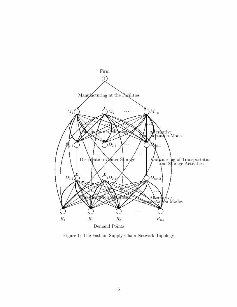
We consider the fashion supply chain network topology depicted in Figure 1 but emphasize

that the modeling framework developed here is not limited to such a network. This network

is only representative, for definiteness. The origin node in the network in Figure 1 consists of

node 1, which represents the beginning of the product processing, and the destination nodes,

R1, . . . , RnR, are the demand points (markets) located at the bottom tier of the network. The

paths joining the origin node to the destination nodes represent sequences of supply chain

network activities corresponding to directed links that ensure that the fashion products are

produced and, ultimately, delivered to the demand points. Hence, different supply chain

network topologies to that depicted in Figure 1 correspond to distinct fashion supply chain

network problems. For example, if the fashion product(s) can be delivered directly to the

demand points from a manufacturing plant, then there would be, as depicted, links joining

the corresponding nodes.

We assume that the fashion producing firm is involved in the production, storage, and

transportation / distribution of J products, with a typical product denoted by j. In particu-

lar, as depicted in Figure 1, we assume that the firm has, at its disposal, nM manufacturing

facilities/plants; nD distribution centers, and must serve the nR demand points. The links

from the top-tiered node are connected to the manufacturing facility nodes of the firm, which

are denoted, respectively, by: M1, . . . ,MnM. The links from the manufacturing facility nodes,

in turn, are connected to the distribution/storage center nodes of the firm, which are de-

noted by D1,1, . . . , DnD,1. Here we allow for the possibility of multiple links joining each such

pair of nodes to reflect possible alternative modes of transportation/shipment between the

manufacturing facilities and the distribution centers, an issue highly relevant to the fashion

industry.

5

mFirm

1�

��

��

��� ?

QQ

QQ

QQ

QQ

QQ

Qs

Manufacturing at the Facilities

M1 M2 MnMm m · · · m

?

@@

@@

@@

@@R

aaaaaaaaaaaaaaaaaaa?

��

��

��

��

QQ

QQ

QQ

QQ

QQ

Qs?

��

��

��

��

��

�+

!!!!!!!!!!!!!!!!!!!

· · · · · ·· · ·· · · · · · · · ·

· · ·· · · · · ·

Transportation/Shipment AlternativeTransportation Modes

· · · · · · · · ·Outsourcing of Transportation

and Storage Activities

D1,1 D2,1 DnD,1m m · · · m

? ? ?D1,2 D2,2 DnD,2

Distribution Center Storage

Transportation/Shipment AlternativeTransportation Modes

m m · · · m���

����������

���

��

��

��

��

AAAAAAAAU

����������������������)

��

��

��

��

��

�+

��

��

��

���

AAAAAAAAU

HHHHHHH

HHHHHHHHj

��

��

��

���

AAAAAAAAU

QQ

QQ

QQ

QQ

QQ

Qs

PPPPPPPPPPPPPPPPPPPPPPq

· · · · · · · · ·· · ·· · ·· · · · · ·

· · ·· · ·· · · · · · · · ·

m m m · · · mR1 R2 R3 RnR

Demand Points

Figure 1: The Fashion Supply Chain Network Topology

6

The links joining nodes D1,1, . . . , DnD,1 with nodes D1,2, . . . , DnD,2 correspond to the

possible storage links for the products. Finally, there are multiple transportation/shipment

links joining the nodes D1,2, . . . , DnD,2 with the demand nodes: R1, . . . , RnR. Distinct such

links also correspond to different modes of transportation/shipment.

The outermost links in Figure 1 can also depict the option of possible outsourcing of the

transportation and storage activities, with appropriate assigned costs and time values, as

will be discussed below. Indeed, our supply chain network framework is sufficiently general

and flexible to also capture alternatives (such as outsourcing of some of the supply chain

network activities) that may be available to the fashion firm.

We assume that in the supply chain network topology there exists one path (or more)

joining node 1 with each destination node. This assumption for the fashion supply chain

network model guarantees that the demand at each demand point will be satisfied. We

denote the supply chain network consisting of the graph G = [N, L], where N denotes the

set of nodes and L the set of directed links.

The demands for the fashion products are assumed as given and are associated with each

product and each demand point. Let djk denote the demand for the product j; j = 1, . . . , J ,

at demand point Rk. A path consists of a sequence of links originating at the top node

and denotes supply chain activities comprising manufacturing, storage, and transporta-

tion/shipment of the products to the demand nodes. Note that, if need be, one can also

add other tiers of nodes and associated links to correspond to import/export administrative

activities. Let xjp denote the nonnegative flow of product j on path p. Let Pk denote the

set of all paths joining the origin node 1 with destination (demand) node Rk. The paths are

assumed to be acyclic.

The following conservation of flow equations must hold for each product j and each

demand point Rk: ∑p∈Pk

xjp = dj

k, j = 1, . . . , J ; k = 1, . . . , nR, (1)

that is, the demand for each product must be satisfied at each demand point.

Links are denoted by a, b, etc. Let f ja denote the flow of product j on link a. We must

have the following conservation of flow equations satisfied:

f ja =

∑p∈P

xjpδap, j = 1, . . . , J ; ∀a ∈ L, (2)

where δap = 1 if link a is contained in path p and δap = 0, otherwise. In other words, the

flow of a product on a link is equal to the sum of flows of the product on paths that contain

7

that link. Here P denotes the set of all the paths in Figure 1. The path flows must be

nonnegative, that is,

xjp ≥ 0, j = 1, . . . , J ; ∀p ∈ P. (3)

We group the path flows into the vector x and the link flows into the vector f , respectively.

Below we present the optimization problems in path flows and in link flows.

There is a unit operational cost associated with each product and each link (cf. Figure

1) of the network. We denote the unit cost on a link a associated with product j by

cja. The unit cost of a link associated with each product, be it a manufacturing link, a

transportation/shipment link, or a storage link, etc., is assumed, for the sake of generality,

to be a function of the flow of all the products on the link. Hence, we have that

cja = cj

a(f1a , . . . , fJ

a ), j = 1, . . . , J ; ∀a ∈ L. (4)

Note that in the case of an outsourcing link for a fashion product the unit cost may be

fixed, as per the negotiated contract.

Let Cjp denote the unit operational cost associated with product j; j = 1, . . . , J , on a

path p, where

Cjp =

∑a∈L

cjaδap, j = 1, . . . , J ; ∀p ∈ P. (5)

Then, the total operational cost for product j; j = 1, . . . , J , on path p; p ∈ P , in view of

(2), (4), and (5), can be expressed as:

Cjp(x) = Cj

p(x)× xjp, j = 1, . . . , J ; ∀p ∈ P. (6)

The total cost minimization problem, hence, is formulated as:

MinimizeJ∑

j=1

∑p∈P

Cjp(x) (7)

subject to constraints (1) and (3).

In addition, the firm also seeks to minimize the time consumption associated with the

demand satisfaction for each product at each demand point. Let tja denote the average unit

time consumption for product j; j = 1, . . . , J , on link a, a ∈ L. We assume that

tja = tja(f1a , . . . , fJ

a ), j = 1, . . . , J, ∀a ∈ L, (8)

that is, the link average unit time consumption is, also, for the sake of generality, a function

of the flow of all the products on that link.

8

Therefore, the average unit time consumption for product j on path p is:

T jp =

∑a∈L

tjaδap, j = 1, . . . , J, ∀p ∈ P, (9)

with the total time consumption for product j on path p, in view of (2), (8), and (9), given

by:

T jp (x) = T j

p (x)× xjp, j = 1, . . . , J ; ∀p ∈ P. (10)

The objective of time minimization problem is to minimize the total time associated

with the supply chain network processing of all the products, which yields the following

optimization problem:

MinimizeJ∑

j=1

∑p∈P

T jp (x), (11)

subject to constraints (1) and (3).

The optimization problems (7) and (11) can be integrated into a single multicriteria

objective function (cf. Dong et al. (2005)) using a weighting factor, ω, representing the

preference of the decision-making authority. Please note that ω here can be interpreted

as the monetary value of a unit of time. Consequently, the multicriteria decision–making

problem, in path flows, can be expressed as:

MinimizeJ∑

j=1

∑p∈P

Cjp(x) + ω

J∑j=1

∑p∈P

T jp (x), (12)

subject to constraints (1) and (3).

The optimization problem (12), with the use of (2), (4), (5), (8), and (9), can be equiva-

lently reformulated in link flows, rather than in path flows, as done above, as:

MinimizeJ∑

j=1

∑a∈L

cja + ω

J∑j=1

∑a∈L

tja, (13)

subject to constraints (1) – (3), where cja ≡ cj

a(f1a , . . . , fJ

a )× f ja and the tja ≡ tja(f

1a , . . . , fJ

a )×f j

a . We assume that the total link cost functions cja and total time functions tja are convex

and continuously differentiable, for all products j and all links a ∈ L.

Let K denote the feasible set such that

K ≡ {x|(1) and (3) are satisfied}. (14)

9

We now state the following result in which we derive the variational inequality formu-

lations of the problem in both path flows and link flows, respectively. Having alternative

formulations allows for the application of distinct algorithms (see, e.g., Nagurney (2006)).

Theorem 1

A path flow vector x∗ ∈ K is an optimal solution to the optimization problem (12), subject

to constraints (1) and (3), if and only if it is a solution to the variational inequality problem

in path flows: determine the vector of optimal path flows, x∗ ∈ K, such that:

J∑j=1

∑p∈P

[∂Cj

p(x∗)

∂xjp

+ w∂T j

p (x∗)

∂xjp

]× (xj

p − xj∗p ) ≥ 0, ∀x ∈ K, (15)

where∂Cj

p(x)

∂xjp

≡∑J

l=1

∑a∈L

∂cla(f1

a ,...,fJa )

∂fja

δap, and∂T j

p (x)

∂xjp

≡∑J

l=1

∑a∈L

∂tla(f1a ,...,fJ

a )

∂fja

δap.

A link flow vector f ∗ ∈ K1 is an optimal solution to the optimization problem (13), subject

to constraints (1) – (3), in turn, if and only if it is a solution to the variational inequality

problem in link flows: determine the vector of optimal link flows, f ∗ ∈ K1, such that:

J∑j=1

J∑l=1

∑a∈L

[∂cl

a(f1∗a , . . . , fJ∗

a )

∂f ja

+ ω∂tla(f

1∗a , . . . , fJ∗

a )

∂f ja

]× (f j

a − f j∗a ) ≥ 0, ∀f ∈ K1, (16)

where K1 ≡ {f |(1)− (3) are satisfied}.

Proof: The result follows from the standard theory of variational inequalities (see the book

by Nagurney (1999) and the references therein) since the functions comprising the objective

functions are convex and continuously differentiable under the imposed assumptions and the

respective feasible sets consisting of the constraints are nonempty, closed, and convex. �

In addition, the following theoretical results in terms of the existence of solutions as

well as the uniqueness of a link flow solution are immediate from the theory of variational

inequalities. Indeed, the existence of solutions to (15) and (16) is guaranteed since the

underlying feasible sets, K and K1, are compact and the corresponding functions of marginal

total costs and marginal total time are continuous, under the above assumptions. If the total

link cost functions and the total time functions are strictly convex, then the solution to (16)

is guaranteed to be unique.

It is worth noting that the above model contains, as a special case, the multiclass system-

optimization transportation network model of Dafermos (1972) if we set ω = 0. The fashion

supply chain management network model developed here is novel since it captures both the

10

reality of multiple products in this application domain as well as the significant relevant

criteria of cost minimization as well as time minimization in the production and delivery of

the fashion products to the demand markets.

Variational inequality (15) can be put into standard form (see Nagurney (1999)): deter-

mine X∗ ∈ K such that:

〈F (X∗)T , X −X∗〉 ≥ 0, ∀X ∈ K, (17)

where 〈·, ·〉 denotes the inner product in n-dimensional Euclidean space. Indeed, if we define

the column vectors: X ≡ x and

F (X) ≡

[∂Cj

p(x)

∂xjp

+ ω∂T j

p (x)

∂xjp

; j = 1, . . . , J ; p ∈ P

], (18)

and K ≡ K then (15) can be re-expressed as (17).

Similarly, if we define the column vectors: X ≡ f and

F (X) ≡[∂cl

a(f1a , . . . , fJ

a )

∂f ja

+ ω∂tla(f

1a , . . . , fJ

a )

∂f ja

; j = 1, . . . , J ; l = 1, . . . , J ; a ∈ L

], (19)

and K ≡ K1 then (16) can be re-expressed as (17).

Note that the above model may be transformed into a single product network model by

making as many copies of the network in Figure 1 as there are products and by construct-

ing appropriate link total cost and time functions, which would be nonseparable, and by

redefining the associated link flows, path flows, and demands accordingly. For details, see

Nagurney and Qiang (2009) and the references therein.

11

R1m mR2

?9

HH

HH

HHj10

?12

��

��

���11

D1,2m mD2,2

?

7?

8

D1,1m mD2,1

?3

HH

HH

HHj4

?6

��

��

���5

M1m mM2

m1Firm

@@

@R1

��

�2

Figure 2: The Supply Chain Network Topology for the Numerical Examples

3. Numerical Examples

We now, for illustration purposes, present fashion supply chain numerical examples, both

single product and multiproduct ones.

3.1 Single Product Fashion Supply Chain Examples

We assume that the fashion firm is involved in the production of a single fashion product

and has, at its disposal, two manufacturing plants and two distribution centers. It must

supply two different demand points. Hence, the topology is as depicted in Figure 2.

The manufacturing plant M1 is located in the U.S., while the manufacturing plant M2 is

located off-shore and has lower operating cost. The average manufacturing time consumption

of one unit of product is identical at these two plants, while the related costs vary mainly

because of the different labor costs. The total cost functions and the total time functions

for all the links are given in Table 1.

The demands for this fashion product at the demand points are:

d1 = 100, d2 = 200,

that is, the market at demand point R1 is half that at demand market R2.

We used the the general equilibration algorithm of Dafermos and Sparrow (1969) (see

also, e.g., Nagurney (1999)) for the solution of the numerical examples.

12

Table 1: Total Link Operational Cost and Total Time Functions

Link a ca(fa) ta(fa)1 10f 2

1 + 10f1 f 21 + 10f1

2 f 22 + 5f2 f 2

2 + 10f2

3 f 23 + 3f3 .5f 2

3 + 5f3

4 f 24 + 4f4 .5f 2

4 + 7f4

5 2f 25 + 30f5 .5f 2

5 + 25f5

6 2f 26 + 20f6 .5f 2

6 + 15f6

7 .5f 27 + 3f7 f 2

7 + 5f7

8 f 28 + 3f8 f 2

8 + 2f8

9 f 29 + 2f9 f 2

9 + 5f9

10 2f 210 + f10 f 2

10 + 3f10

11 f 211 + 5f11 f 2

11 + 2f11

12 f 212 + 4f12 f 2

12 + 4f12

We conducted sensitivity analysis by varying the value of time, ω, for ω = 0, 1, 2, 3, 4, 5.

The computed optimal link flows are reported in Table 2.

We now display the optimal link flows as ω varies for the manufacturing links in Figure

3; for the first set of transportation links in Figure 4; for the set of storage links in Figure 5,

and for the bottom tier of transportation links in Figure 6.

It is interesting to note from Figure 3 that, with the increase of the value of time, part of

the fashion production is shifted from offshore manufacturing plant M2 to onshore facility

M1, due to the onshore facility’s advantage of shorter transportation time to distribution

centers (or demand markets). Consequently, there is an increase in transportation flow from

the onshore facility M1 to the distribution centers, as depicted in Figure 4. Figure 5, in

turn, illustrates that distribution center D2 is getting to be an appealing choice as the time

performance concern increases, although the storage cost there is slightly higher than at D1.

Also, as the value of time increases, a volume of the fashion product flow switches from

transportation link 9 (or link 12) to transportation link 11 (or link 10), to reduce the total

time consumption of the distribution activities (as shown in Figure 6).

13

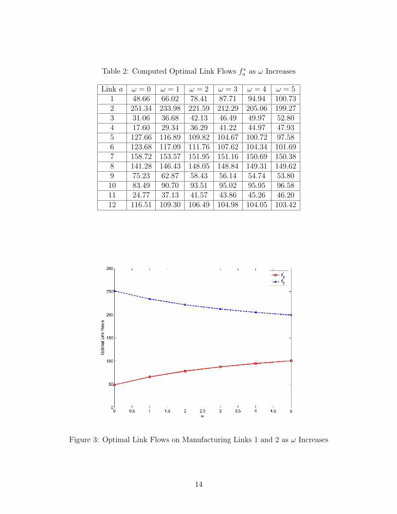
Table 2: Computed Optimal Link Flows f ∗a as ω Increases

Link a ω = 0 ω = 1 ω = 2 ω = 3 ω = 4 ω = 51 48.66 66.02 78.41 87.71 94.94 100.732 251.34 233.98 221.59 212.29 205.06 199.273 31.06 36.68 42.13 46.49 49.97 52.804 17.60 29.34 36.29 41.22 44.97 47.935 127.66 116.89 109.82 104.67 100.72 97.586 123.68 117.09 111.76 107.62 104.34 101.697 158.72 153.57 151.95 151.16 150.69 150.388 141.28 146.43 148.05 148.84 149.31 149.629 75.23 62.87 58.43 56.14 54.74 53.8010 83.49 90.70 93.51 95.02 95.95 96.5811 24.77 37.13 41.57 43.86 45.26 46.2012 116.51 109.30 106.49 104.98 104.05 103.42

Figure 3: Optimal Link Flows on Manufacturing Links 1 and 2 as ω Increases

14

Figure 4: Optimal Link Flows on Transportation Links 3, 4, 5, and 6 as ω Increases

Figure 5: Optimal Link Flows on Storage Links 7 and 8 as ω Increases

15

Figure 6: Optimal Link Flows on Transportation Links 9, 10, 11, and 12 as ω Increases

Table 3: Total Costs and Total Times as ω Increases

ω = 0 ω = 1 ω = 2 ω = 3 ω = 4 ω = 5Total cost 227, 590.89 231, 893.93 239, 656.04 247, 949.30 255, 864.62 263, 121.79Total time 164, 488.11 154, 652.53 149, 329.07 145, 965.20 143, 684.11 142, 061.79

In Table 3, we provide the values of the total costs and the total time at the optimal

solutions for the examples as ω increases.

The values of the minimal total costs and the minimal total time for varying ω are

displayed graphically in Figure 7. As can be seen from Figure 7, as the weight ω increases

the minimal total time decreases, as expected, since a higher value of ω represents an increase

in the decision-maker’s valuation of time as a criterion.

3.2 Multiproduct Fashion Supply Chain Examples

We then considered multiproduct fashion supply chain problems. We assumed that the

fashion firm provides two different fashion products with the same supply chain network

topology as depicted in Figure 2. The total cost functions and the total time functions for

16

Figure 7: Minimal Total Costs and Minimal Total Times as ω Increases

all the links associated with product 1 and product 2 are given in Table 4 and 5, respectively.

The demands for the two fashion products at the demand points are:

d11 = 100, d1

2 = 200, d21 = 300, d2

2 = 400.

To solves these problems, we used the modified projection method of Korpelevich (1977),

embedded with the general equilibration algorithm of Dafermos and Sparrow (1969) (see

also, e.g., Nagurney (1999)).

We also conducted sensitivity analysis, as in Section 3.1, by varying the value of time,

ω, for ω = 0, 1, 2, 3, 4, 5. The computed optimal link flows associated with products 1 and 2

are, respectively, reported in Tables 6 and 7.

We display the optimal link flows of products 1 and 2 as ω varies for the manufacturing

links in Figure 8; for the first set of transportation links in Figure 9; for the set of storage

links in Figure 10, and for the bottom tier of transportation links in Figure 11.

With the increase of the value of time, parts of the production of fashion products 1 and 2

are shifted from offshore manufacturing plant M2 to onshore facility M1 (as depicted in Figure

8), resulting in an increase in transportation flow from M1 to the distribution centers for both

17

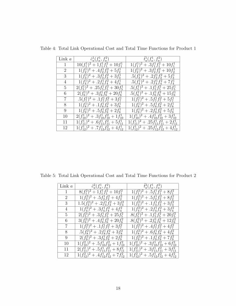
Table 4: Total Link Operational Cost and Total Time Functions for Product 1

Link a c1a(f

1a , f2

a ) t1a(f1a , f2

a )1 10(f 1

1 )2 + 1f 11 f 2

1 + 10f 11 1(f 1

1 )2 + .3f 11 f 2

1 + 10f 11

2 1(f 12 )2 + .4f 1

2 f 22 + 5f 1

2 1(f 12 )2 + .3f 1

2 f 22 + 10f 1

2

3 1(f 13 )2 + .3f 1

3 f 23 + 3f 1

3 .5(f 13 )2 + .2f 1

3 f 23 + 5f 1

3

4 1(f 14 )2 + .2f 1

4 f 24 + 4f 1

4 .5(f 14 )2 + .2f 1

4 f 24 + 7f 1

4

5 2(f 15 )2 + .25f 1

5 f 25 + 30f 1

5 .5(f 15 )2 + .1f 1

5 f 25 + 25f 1

5

6 2(f 16 )2 + .3f 1

6 f 26 + 20f 1

6 .5(f 16 )2 + .1f 1

6 f 26 + 15f 1

6

7 .5(f 17 )2 + .1f 1

7 f 27 + 3f 1

7 1(f 17 )2 + .5f 1

7 f 27 + 5f 1

7

8 1(f 18 )2 + .1f 1

8 f 28 + 3f 1

8 1(f 18 )2 + .5f 1

8 f 28 + 2f 1

8

9 1(f 19 )2 + .5f 1

9 f 29 + 2f 1

9 1(f 19 )2 + .2f 1

9 f 29 + 5f 1

9

10 2(f 110)

2 + .3f 110f

210 + 1f 1

10 1(f 110)

2 + .4f 110f

210 + 3f 1

10

11 1(f 111)

2 + .6f 111f

211 + 5f 1

11 1(f 111)

2 + .25f 111f

211 + 2f 1

11

12 1(f 112)

2 + .7f 112f

212 + 4f 1

12 1(f 112)

2 + .25f 112f

212 + 4f 1

12

Table 5: Total Link Operational Cost and Total Time Functions for Product 2

Link a c2a(f

1a , f2

a ) t2a(f1a , f2

a )1 8(f 2

1 )2 + 1f 11 f 2

1 + 10f 21 1(f 2

1 )2 + .5f 11 f 2

1 + 8f 21

2 1(f 22 )2 + .5f 1

2 f 22 + 4f 2

2 1(f 22 )2 + .5f 1

2 f 22 + 8f 2

2

3 1.5(f 23 )2 + .2f 1

3 f 23 + 3f 2

3 1(f 23 )2 + .1f 1

3 f 23 + 3f 2

3

4 1(f 24 )2 + .3f 1

4 f 24 + 4f 2

4 1(f 24 )2 + .2f 1

4 f 24 + 3f 2

4

5 2(f 25 )2 + .3f 1

5 f 25 + 25f 2

5 .8(f 25 )2 + .1f 1

5 f 25 + 20f 2

5

6 3(f 26 )2 + .4f 1

6 f 26 + 20f 2

6 .8(f 26 )2 + .2f 1

6 f 26 + 12f 2

6

7 1(f 27 )2 + .1f 1

7 f 27 + 3f 2

7 1(f 27 )2 + .4f 1

7 f 27 + 4f 2

7

8 .5(f 28 )2 + .2f 1

8 f 28 + 3f 2

8 1(f 28 )2 + .6f 1

8 f 28 + 4f 2

8

9 2(f 29 )2 + .3f 1

9 f 29 + 2f 2

9 1(f 29 )2 + .1f 1

9 f 29 + 7f 2

9

10 1(f 210)

2 + .5f 110f

210 + 1f 2

10 1(f 210)

2 + .3f 110f

210 + 6f 2

10

11 2(f 211)

2 + .5f 111f

211 + 8f 2

11 1(f 211)

2 + .3f 111f

211 + 3f 2

11

12 1(f 212)

2 + .4f 112f

212 + 7f 2

12 1(f 212)

2 + .5f 112f

212 + 4f 2

12

18

Table 6: Computed Optimal Link Flows f 1∗a as ω Increases for Product 1

Link a ω = 0 ω = 1 ω = 2 ω = 3 ω = 4 ω = 51 53.81 71.31 83.38 92.24 99.02 104.392 246.19 228.69 216.62 207.76 200.98 195.613 41.58 43.44 47.03 50.23 52.90 55.104 12.23 27.87 36.35 42.01 46.13 49.295 125.73 114.20 106.97 101.86 98.02 95.016 120.45 114.49 109.64 105.90 102.96 100.607 167.32 157.64 154.00 152.09 150.91 150.118 132.68 142.36 146.00 147.91 149.09 149.899 73.27 63.60 60.07 58.25 57.14 56.3910 94.05 94.04 93.93 93.84 93.78 93.7311 26.73 36.40 39.93 41.75 42.86 43.6112 105.95 105.96 106.07 106.16 106.22 106.27

Table 7: Computed Optimal Link Flows f 2∗a as ω Increases for Product 2

Link a ω = 0 ω = 1 ω = 2 ω = 3 ω = 4 ω = 51 150.04 192.14 219.13 237.85 251.58 262.072 549.96 507.86 480.87 462.15 448.42 437.933 17.38 63.50 87.28 102.35 112.87 120.654 132.66 128.64 131.85 135.50 138.71 141.425 309.57 278.09 259.11 246.45 237.40 230.616 240.39 229.77 221.75 215.70 211.02 207.327 326.95 341.59 346.39 348.80 350.27 351.268 373.05 358.41 353.61 351.20 349.73 348.749 141.99 145.71 147.19 148.00 148.52 148.8810 184.96 195.88 199.20 200.80 201.75 202.3811 158.01 154.29 152.81 152.00 151.48 151.1212 215.04 204.12 200.80 199.20 198.25 197.62

19

Figure 8: Optimal Link Flows on Manufacturing Links 1 and 2 as ω Increases

Figure 9: Optimal Link Flows on Transportation Links 3, 4, 5, and 6 as ω Increases

20

Figure 10: Optimal Link Flows on Storage Links 7 and 8 as ω Increases

Figure 11: Optimal Link Flows on Transportation Links 9, 10, 11, and 12 as ω Increases

21

Table 8: Total Costs and Total Times as ω Increases

ω = 0 ω = 1 ω = 2 ω = 3 ω = 4 ω = 5Total cost 1, 722, 082.05 1, 745, 201.77 1, 788, 457.21 1, 831, 689.80 1, 870, 523.21 1, 904, 398.75Total time 1, 291, 094.62 1, 222, 959.73 1, 189, 192.37 1, 169, 656.19 1, 157, 297.60 1, 148, 975.34

Figure 12: Minimal Total Costs and Minimal Total Times as ω Increases

fashion products (as shown in Figure 9). However, Figure 10 illustrates that the distribution

center D2 is getting to be appealing for product 1 as the value of time increases, while the

distribution center D1 becomes attractive for product 2, since the distribution center D1 is

more time-efficient for product 2. In Figure 11, as the time performance concern increases, a

volume of fashion product 1 switches from transportation link 9 to link 11; in contrast, the

volume of flow of fashion product 2 on link 9 increases. Also, a volume of fashion product

2 switches from link 12 to link 10, while the flows of fashion product 1 on link 10 and 12

change slightly.

The values of the total costs and the total time at the optimal solutions for the examples

as ω increases are provided in Table 8, and displayed graphically in Figure 12. As expected,

the minimal total time decreases as ω increases.

22

4. Summary and Conclusions and Suggestions for Future Research

In this paper, we developed a fashion supply chain management model, using a network

economics perspective, that allows for multiple fashion products. The model consists of two

objective functions: total cost minimization, associated with supply chain network activities,

in the form of: manufacturing, storage, and distribution, and total time consumption min-

imization. A weighted objective function was then constructed with the weighting factor,

representing the monetary value of a unit of time, decided by the firm.

We also provided the optimization model’s equivalent variational inequality formulation,

with nice features for computational purposes. The solution of the model yields the opti-

mal multiproduct fashion flows of supply chain network activities, with the demands being

satisfied at the minimal total cost and the minimal total time consumption. The model

is illustrated with a spectrum of numerical examples with potential application to fashion

supply chain management.

The fashion supply chain network model allows the cognizant decision-maker to evaluate

the effects of changes in the demand for its products on the total operations costs and time.

It allows for the evaluation of changes in the cost functions and the time functions on total

supply chain network costs and time. In addition, the flexibility of the network framework

allows for the evaluation of the addition of various links (or their removal) on the values of

the objective function(s). Finally, the model, since it is network-based, is visually graphic.

The research in this paper can be extended in several directions. One can construct a fash-

ion supply chain management model with price-sensitive and time-sensitive demands under

oligopolistic competition. One can also incorporate environmental concerns and associated

trade-offs. In addition, one can explore computationally as well as empirically large-scale

fashion supply chain networks within our modeling framework. We leave such research for

the future.

Acknowledgments The authors acknowledge the helpful comments and suggestions of two

anonymous reviewers. The authors also thank Professor Jason Choi for the opportunity to

contribute to his edited volume.

This research was supported, in part, by the John F. Smith Memorial Fund. This support

is gratefully acknowledged.

References

Arntzen, B. C., Brown, G. G., Harrison, T. P., & Trafton L. L. (1995). Global supply chain

23

management at Digital Equipment Corporation. Interfaces, 25(1), 69-93.

Bower, J. L., & Hout, T. M. (1988). Fast cycle capability for competitive power. Harvard

Business Review, 88(6), 110-118,

Cheong, M. L. F., Bhatnagar, R., & Graves, S.C. (2004). Logistics network deign with differ-

entiated delivery lead-time: Benefits and insights. http://web.mit.edu/sgraves/www/papers/

Cheong1119.pdf, accessed on June 8th, 2010.

Christopher, M. (1992). Logistics and Supply Chain Management, London: Pitman Publish-

ing.

Dafermos, S. C. (1972). The traffic assignment problem for multiclass-user transportation

networks. Transportation Science, 6(1), 73-87.

Dafermos, S. C., & Sparrow, F. T. (1969). The traffic assignment problem for a general

network. Journal of Research of the National Bureau of Standards , 73B, 91-118.

Doeringer, P., & Crean, S. (2006). Can fast fashion save the U.S. apparel industry? Socio-

Economic Review, 4(3), 353-377.

Dong, J., Zhang, D., Yan, H., & Nagurney, A. (2005). Multitiered supply chain networks:

multicriteria decision-making under uncertainty, Annals of Operations Research, 135(1), 155-

178.

Ferdows, K., Lewis, M. A., & Machuca, J. A. D.(2004). Rapid-fire fulfillment. Harvard

Business Review , 82(11), 104-110.

Fisher, M. L. (1997). What is the right supply chain for your product? Harvard Business

Review , 75(2), 105-116.

Goetschalckx, M., Vidal, C. J., & Dogan, K. (2002). Modeling and design of global logis-

tics systems: A review of integrated strategic and tactical models and design algorithms.

European Journal of Operational Research, 143(1), 1-18.

Guide Jr., V. D. R., Muyldermans, L., & Van Wassenhove, L. N. (2005). Hewlett-Packard

Company unlocks the value potential from time-sensitive returns. Interfaces, 35(4), 281-293.

Gunasekaran, A., Patel, C., & McGaughey, R. E. (2004). A framework for supply chain

performance measurement. International Journal of Production Economics, 87(3), 333-347.

24

Gunasekaran, A., Patel, C., & Tirtiroglu, E. (2001). Performance measures and metrics in a

supply chain environment. International Journal of Operations and Production Management,

21(1/2), 71-87.

Ho, W., Xu, X., & Dey, P. K. (2010). Multi-criteria decision making approaches for supplier

evaluation and selection: A literature review. European Journal of Operational Research,

202(1), 16-24.

Korpelevich, G. M. (1977). The extragradient method for finding saddle points and other

problems. Matekon, 13, 35-49.

Lederer, P.J., & Li, L. (1997). Pricing, production, scheduling, and delivery-time competi-

tion. Operations Research, 45(3), 407-420.

Liu, L., Parlar, M., & Zhu, S. X. (2007). Pricing and lead time decisions in decentralized

supply chains. Management Science, 53(5), 713-725.

Nagurney, A. (1999). Network Economics: A Variational Inequality Approach, second and

revised edition. Boston, Massachusetts: Kluwer Academic Publishers.

Nagurney, A. (2006). Supply Chain Network Economics: Dynamics of Prices, Flows, and

Profits. Cheltenham, England: Edward Elgar Publishing.

Nagurney, A. (2010). Supply chain network design under profit maximization and oligopolis-

tic competition. Transportation Research E, 46(3), 281-294.

Nagurney, A., Cruz, J., Dong, J., & Zhang, D. (2005). Supply chain networks, electronic

commerce, and supply side and demand side risk. European Journal of Operational Research,

164(1), 120-142.

Nagurney, A., & Matsypura, D. (2005). Global supply chain network dynamics with mul-

ticriteria decision-making under risk and uncertainty. Transportation Research E, 41(6),

585-612.

Nagurney, A., & Nagurney, L. S. (2010). Sustainable supply chain network design: A mul-

ticriteria perspective. International Journal of Sustainable Engineering, 3(3), 189-197.

Nagurney, A., & Qiang, Q. (2009). Fragile Networks: Identifying Vulnerabilities and Syner-

gies in an Uncertain World . Hoboken, New Jersey: John Wiley & Sons.

Nagurney, A., & Woolley, T. (2010). Environmental and cost synergy in supply chain network

25

integration in mergers and acquisitions. In M. Ehrgott, B. Naujoks, T. Stewart, and J.

Wallenius (Eds.), Sustainable Energy and Transportation Systems, Proceedings of the 19th

International Conference on Multiple Criteria Decision Making, Lecture Notes in Economics

and Mathematical Systems (pp. 51-78). Berlin, Germany: Springer.

Nordas, H. K., Pinali, E., & Geloso Grosso, M. (2006). Logistics and time as a trade barrier.

OECD Trade Policy Working Papers, No. 35, OECD Publishing. doi:10.1787/664220308873.

Palaka, K., Erlebacher, S., & Kropp D. H. (1998). Lead-time setting, capacity utilization,

and pricing decisions under lead-time dependent demand. IIE Transactions, 30(2), 151-163.

Ray, S., & Jewkes, E. M. (2004). Customer lead time management when both demand and

price are lead time sensitive. European Journal of Operational Research, 153(3), 769-781.

Sen, A. (2008). The US fashion industry: A supply chain review. International Journal of

Production Economics, 114(2), 571-593.

So, K. C (2000). Price and time competition for service delivery. Manufacturing and Service

Operations Management, 2(4), 392-409.

So, K. C., & Song, J. S. (1998). Price, delivery time guarantees and capacity selection,

European Journal of Operational Research, 111(1), 28-49.

Sull, D., & Turconi, S. (2008). Fast fashion lessons. Business Strategy Review, Summer,

5-11.

Towill, D. R. (1997). The seamless supply chain – the predator’s strategic advantage. In-

ternational Journal of Technology Management, 13(1), 37-56.

26