fast agglomerative clustering for rendering bruce walter, kavita bala, cornell university milind...
Post on 21-Dec-2015
223 views
TRANSCRIPT
Fast Agglomerative Clustering for Rendering
Fast Agglomerative Clustering for Rendering
Bruce Walter, Kavita Bala,
Cornell University
Milind Kulkarni, Keshav Pingali
University of Texas, Austin
2
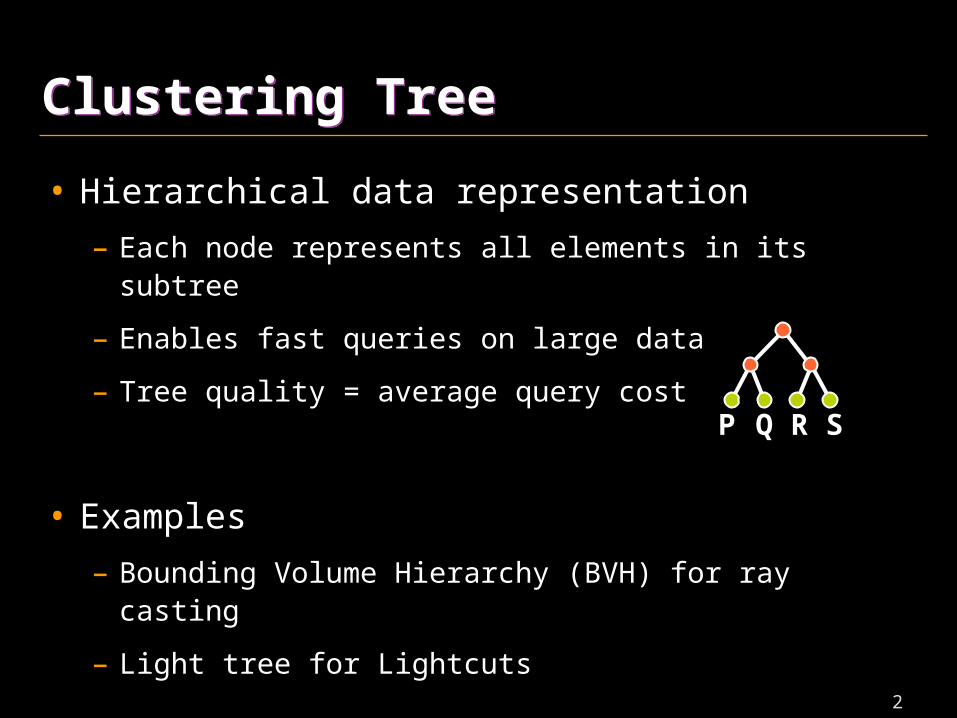
Clustering TreeClustering Tree
• Hierarchical data representation
– Each node represents all elements in its subtree
– Enables fast queries on large data
– Tree quality = average query cost
• Examples
– Bounding Volume Hierarchy (BVH) for ray casting
– Light tree for Lightcuts
P Q R S
3
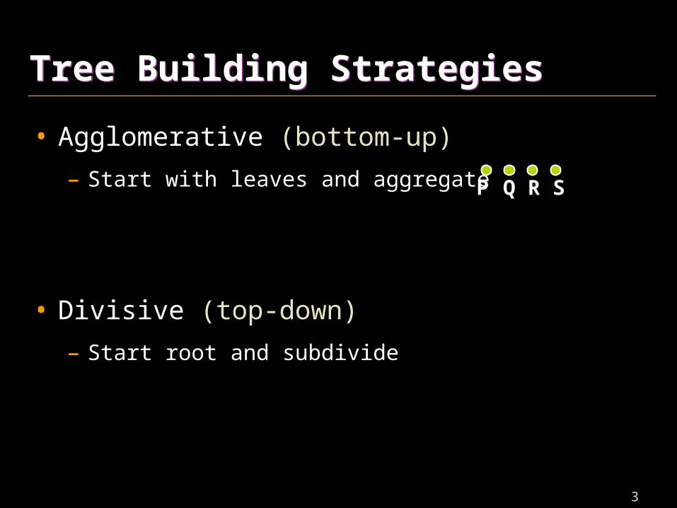
Tree Building StrategiesTree Building Strategies
• Agglomerative (bottom-up)
– Start with leaves and aggregate
• Divisive (top-down)
– Start root and subdivide
P Q R S
4
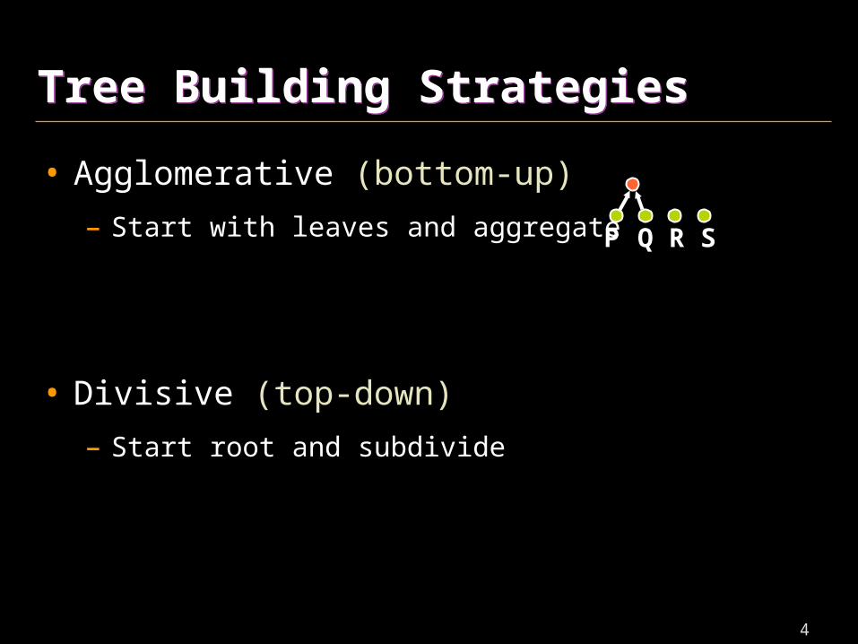
Tree Building StrategiesTree Building Strategies
• Agglomerative (bottom-up)
– Start with leaves and aggregate
• Divisive (top-down)
– Start root and subdivide
P Q R S
5
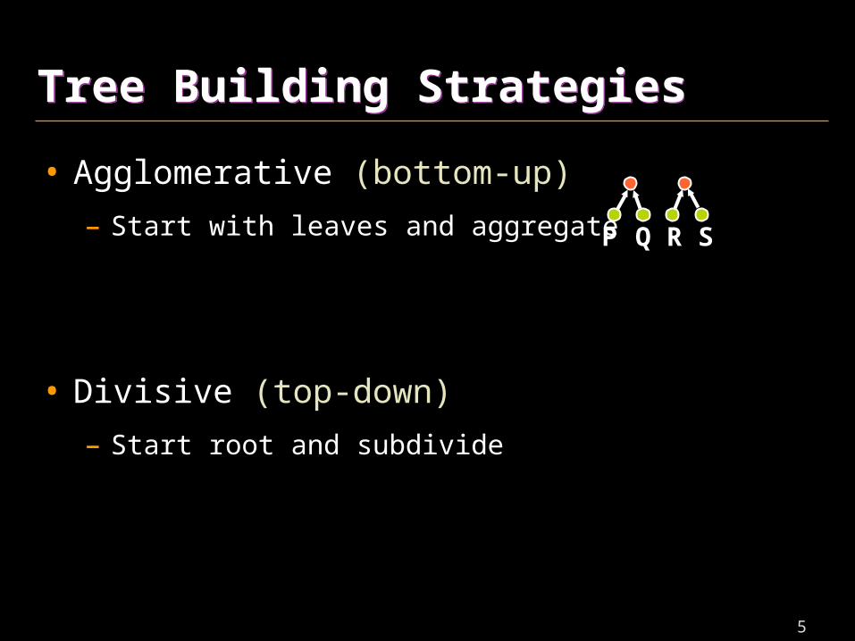
Tree Building StrategiesTree Building Strategies
• Agglomerative (bottom-up)
– Start with leaves and aggregate
• Divisive (top-down)
– Start root and subdivide
P Q R S
6
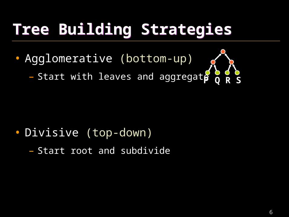
Tree Building StrategiesTree Building Strategies
• Agglomerative (bottom-up)
– Start with leaves and aggregate
• Divisive (top-down)
– Start root and subdivide
P Q R S
7
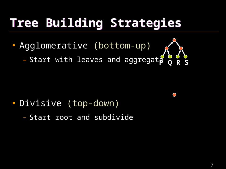
Tree Building StrategiesTree Building Strategies
• Agglomerative (bottom-up)
– Start with leaves and aggregate
• Divisive (top-down)
– Start root and subdivide
P Q R S
8
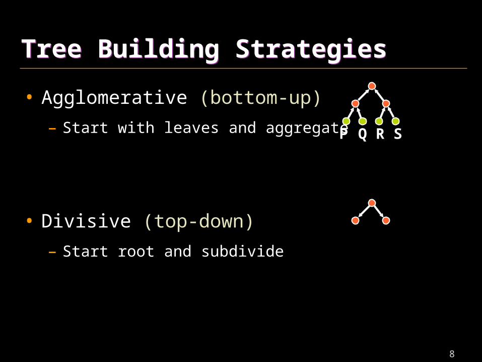
Tree Building StrategiesTree Building Strategies
• Agglomerative (bottom-up)
– Start with leaves and aggregate
• Divisive (top-down)
– Start root and subdivide
P Q R S
9
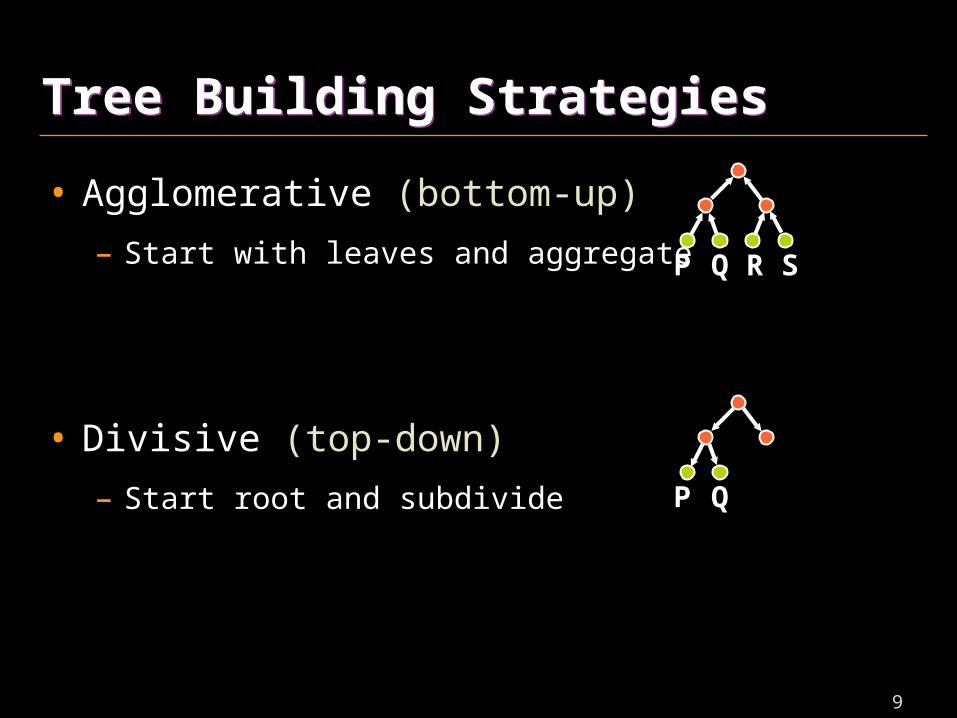
Tree Building StrategiesTree Building Strategies
• Agglomerative (bottom-up)
– Start with leaves and aggregate
• Divisive (top-down)
– Start root and subdivide
P Q R S
P Q
10
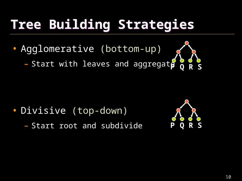
Tree Building StrategiesTree Building Strategies
• Agglomerative (bottom-up)
– Start with leaves and aggregate
• Divisive (top-down)
– Start root and subdivide
P Q R S
P Q R S
11
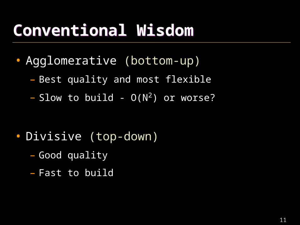
Conventional WisdomConventional Wisdom
• Agglomerative (bottom-up)
– Best quality and most flexible
– Slow to build - O(N2) or worse?
• Divisive (top-down)
– Good quality
– Fast to build
12
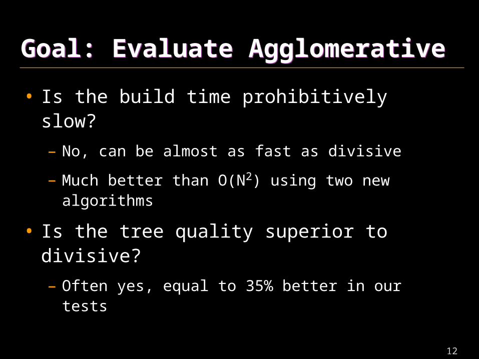
Goal: Evaluate AgglomerativeGoal: Evaluate Agglomerative
• Is the build time prohibitively slow?
– No, can be almost as fast as divisive
– Much better than O(N2) using two new algorithms
• Is the tree quality superior to divisive?
– Often yes, equal to 35% better in our tests
13
Related WorkRelated Work• Agglomerative clustering
– Used in many different fields including data mining, compression, and bioinformatics [eg, Olson 95, Guha et al. 95, Eisen et al. 98, Jain et al. 99, Berkhin 02]
• Bounding Volume Hierarchies (BVH)– [eg, Goldsmith and Salmon 87, Wald et al. 07]
• Lightcuts– [eg, Walter et al. 05, Walter et al. 06, Miksik 07, Akerlund
et al. 07, Herzog et al. 08]
14
OverviewOverview
• How to implement agglomerative clustering
– Naive O(N3) algorithm
– Heap-based algorithm
– Locally-ordered algorithm
• Evaluating agglomerative clustering
– Bounding volume hierarchies
– Lightcuts
• Conclusion
15
Agglomerative BasicsAgglomerative Basics
• Inputs
– N elements
– Dissimilarity function, d(A,B)
• Definitions
– A cluster is a set of elements
– Active cluster is one that is not yet part of a larger cluster
• Greedy Algorithm
– Combine two most similar active clusters and repeat
16
Dissimilarity FunctionDissimilarity Function
• d(A,B): pairs of clusters real number
– Measures “cost” of combining two clusters
– Assumed symmetric but otherwise arbitrary
– Simple examples:
• Maximum distance between elements in A+B
• Volume of convex hull of A+B
• Distance between centroids of A and B
17
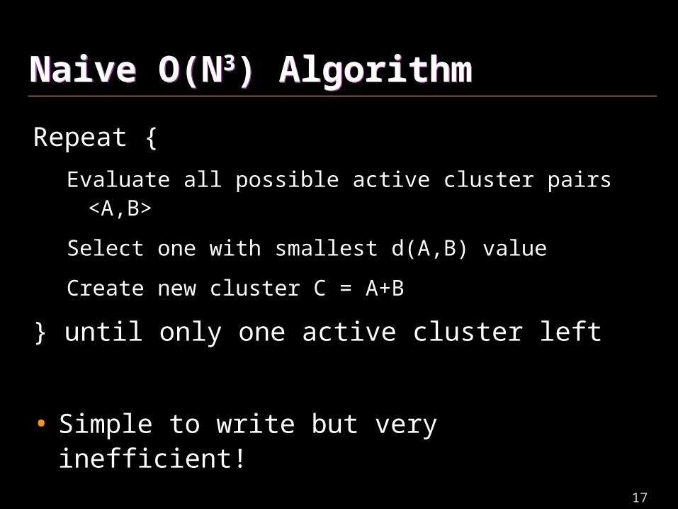
Naive O(N3) AlgorithmNaive O(N3) Algorithm
Repeat {
Evaluate all possible active cluster pairs <A,B>
Select one with smallest d(A,B) value
Create new cluster C = A+B
} until only one active cluster left
• Simple to write but very inefficient!
18
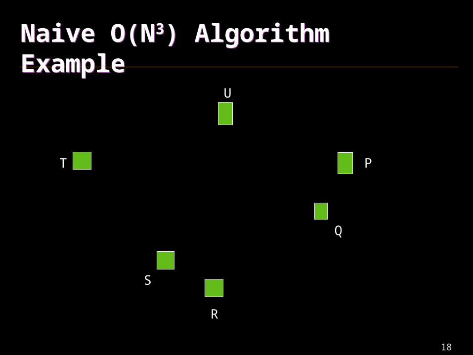
Naive O(N3) Algorithm ExampleNaive O(N3) Algorithm Example
P
U
Q
R
T
S
19
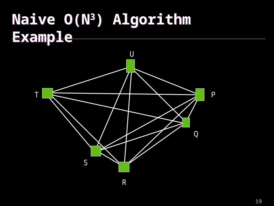
Naive O(N3) Algorithm ExampleNaive O(N3) Algorithm Example
P
U
Q
R
T
S
20
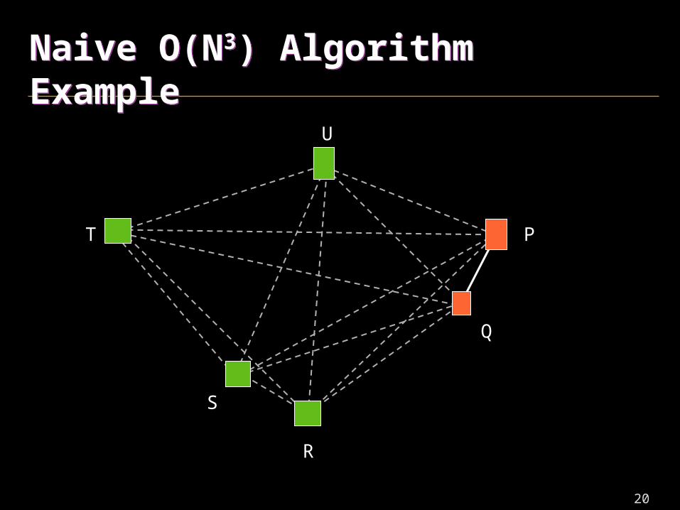
Naive O(N3) Algorithm ExampleNaive O(N3) Algorithm Example
P
U
Q
R
T
S
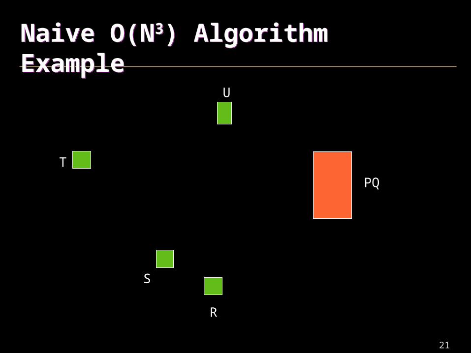
21
Naive O(N3) Algorithm ExampleNaive O(N3) Algorithm Example
PQ
U
R
T
S
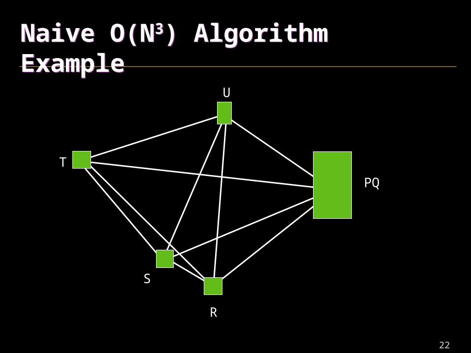
22
Naive O(N3) Algorithm ExampleNaive O(N3) Algorithm Example
PQ
U
R
T
S
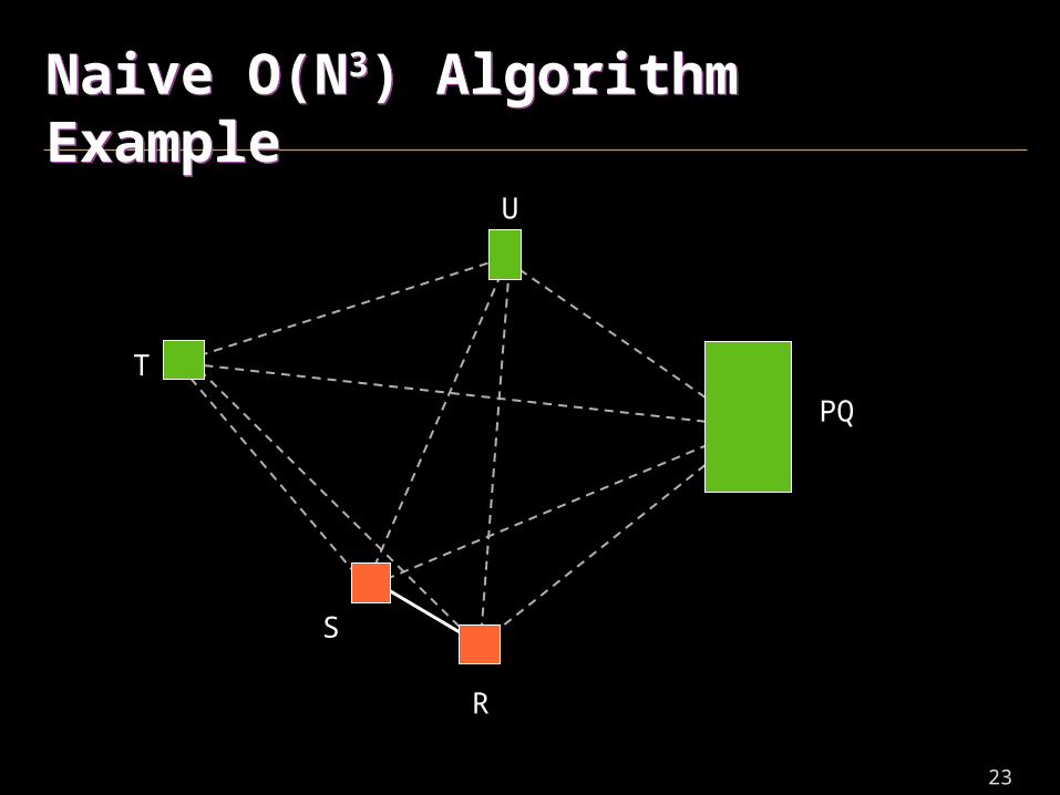
23
Naive O(N3) Algorithm ExampleNaive O(N3) Algorithm Example
PQ
U
R
T
S
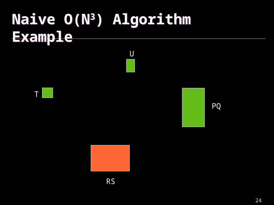
24
Naive O(N3) Algorithm ExampleNaive O(N3) Algorithm Example
PQ
U
RS
T
25
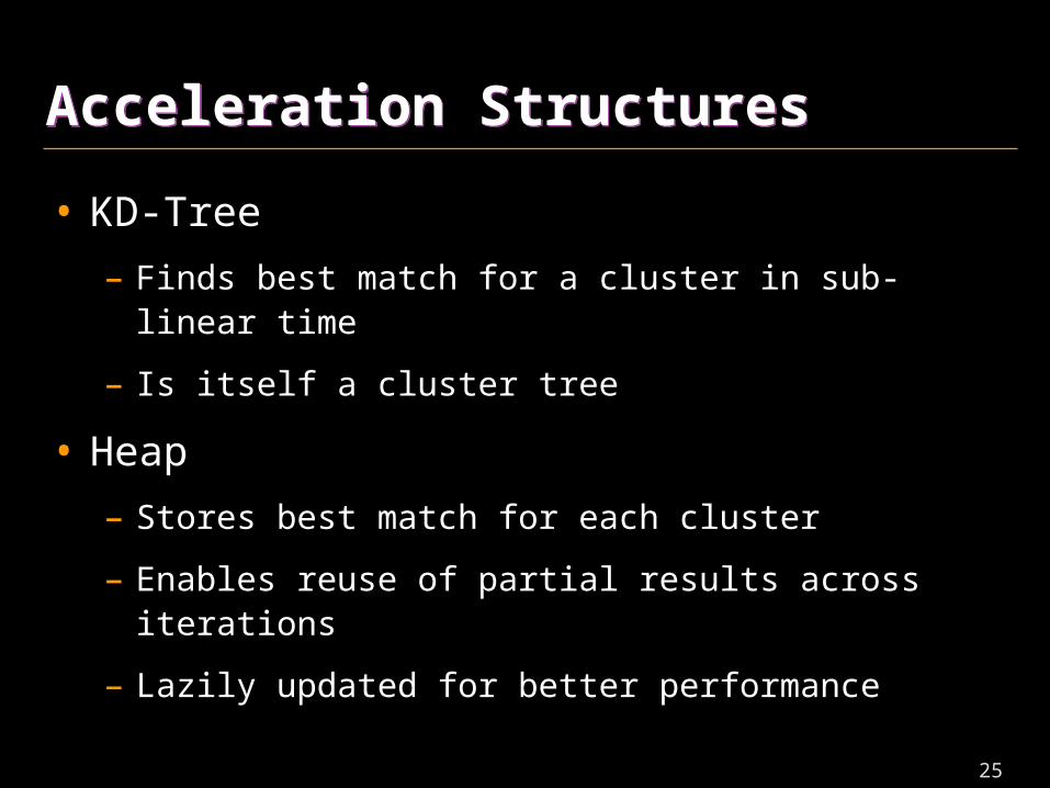
Acceleration StructuresAcceleration Structures
• KD-Tree
– Finds best match for a cluster in sub-linear time
– Is itself a cluster tree
• Heap
– Stores best match for each cluster
– Enables reuse of partial results across iterations
– Lazily updated for better performance
26
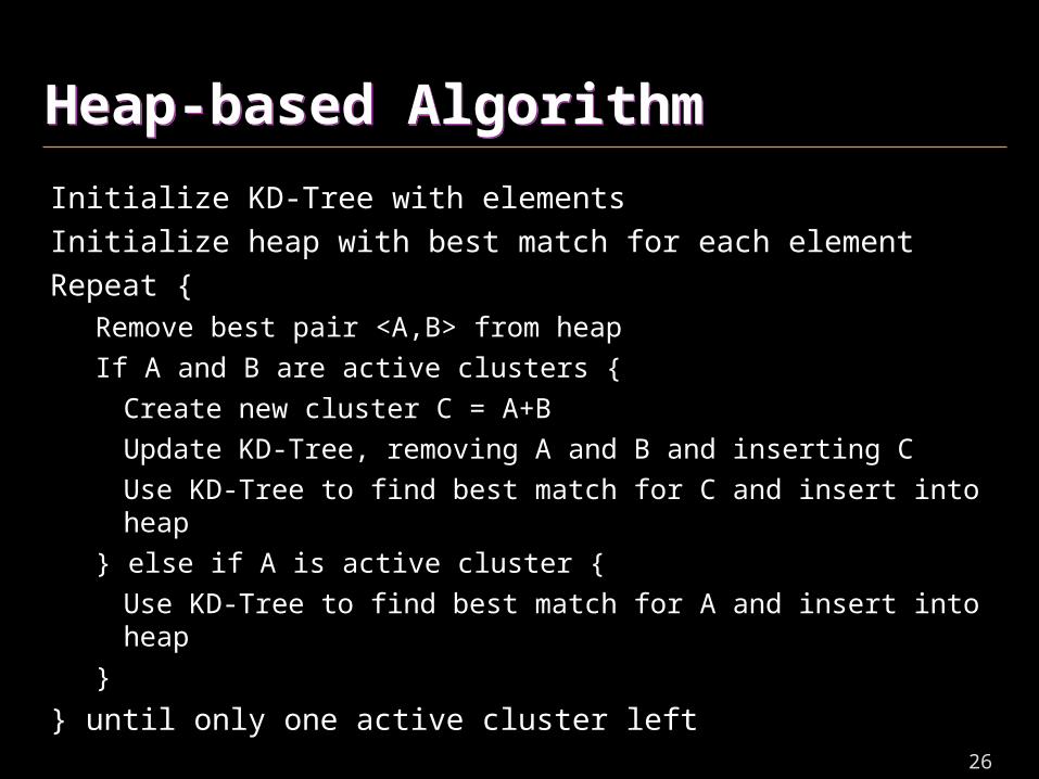
Heap-based AlgorithmHeap-based Algorithm
Initialize KD-Tree with elements
Initialize heap with best match for each element
Repeat {Remove best pair <A,B> from heap
If A and B are active clusters {
Create new cluster C = A+B
Update KD-Tree, removing A and B and inserting C
Use KD-Tree to find best match for C and insert into heap
} else if A is active cluster {
Use KD-Tree to find best match for A and insert into heap
}
} until only one active cluster left
27
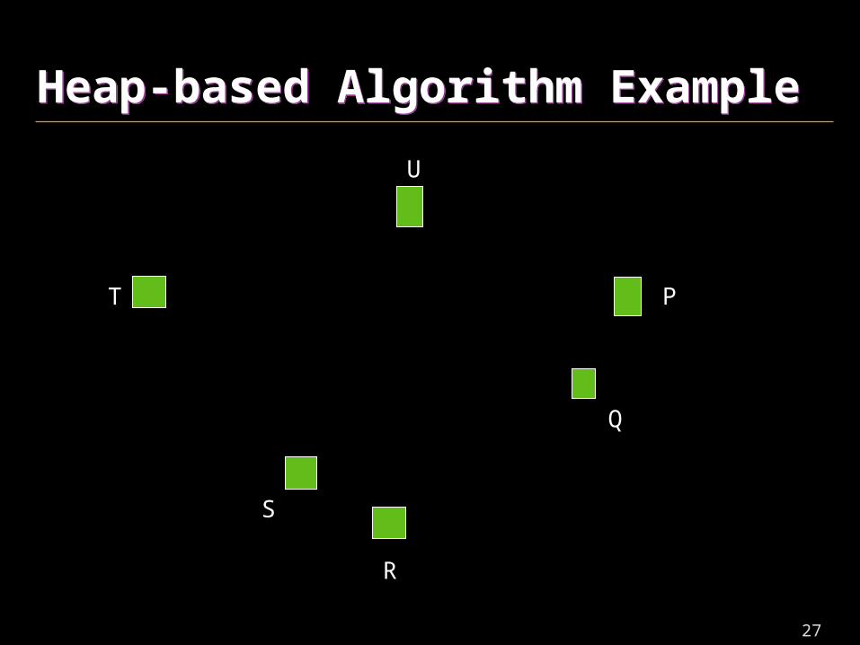
Heap-based Algorithm ExampleHeap-based Algorithm Example
P
U
Q
R
T
S
28
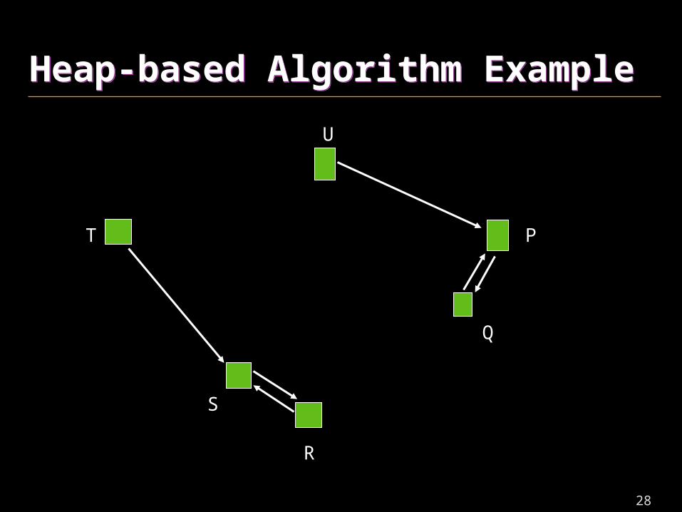
Heap-based Algorithm ExampleHeap-based Algorithm Example
P
U
Q
R
T
S
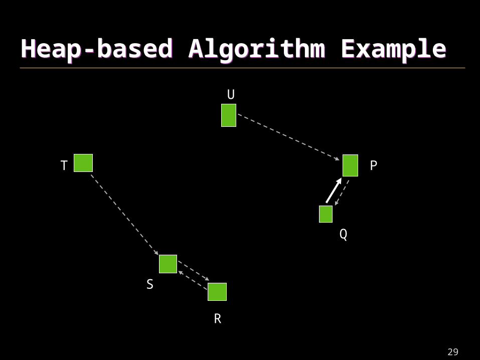
29
Heap-based Algorithm ExampleHeap-based Algorithm Example
P
U
Q
R
T
S

30
Heap-based Algorithm ExampleHeap-based Algorithm Example
U
R
T
S
PQ
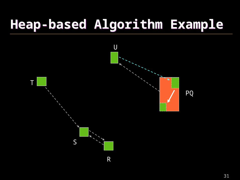
31
Heap-based Algorithm ExampleHeap-based Algorithm Example
PQ
U
R
T
S

32
Heap-based Algorithm ExampleHeap-based Algorithm Example
PQ
U
R
T
S
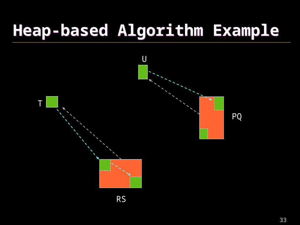
33
Heap-based Algorithm ExampleHeap-based Algorithm Example
PQ
U
RS
T
34
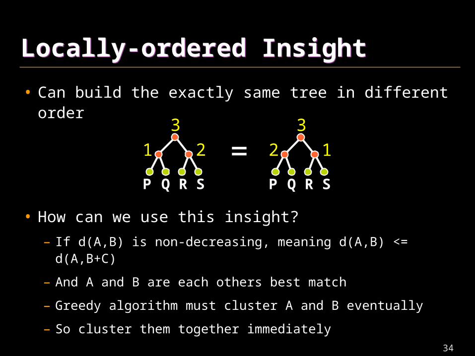
Locally-ordered InsightLocally-ordered Insight
• Can build the exactly same tree in different order
• How can we use this insight?
– If d(A,B) is non-decreasing, meaning d(A,B) <= d(A,B+C)
– And A and B are each others best match
– Greedy algorithm must cluster A and B eventually
– So cluster them together immediately
P Q R S
1 2
3
P Q R S
2 1
3
=
35
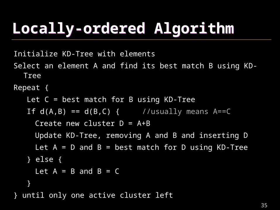
Locally-ordered AlgorithmLocally-ordered Algorithm
Initialize KD-Tree with elements
Select an element A and find its best match B using KD-Tree
Repeat {
Let C = best match for B using KD-Tree
If d(A,B) == d(B,C) { //usually means A==C
Create new cluster D = A+B
Update KD-Tree, removing A and B and inserting D
Let A = D and B = best match for D using KD-Tree
} else {
Let A = B and B = C
}
} until only one active cluster left
36
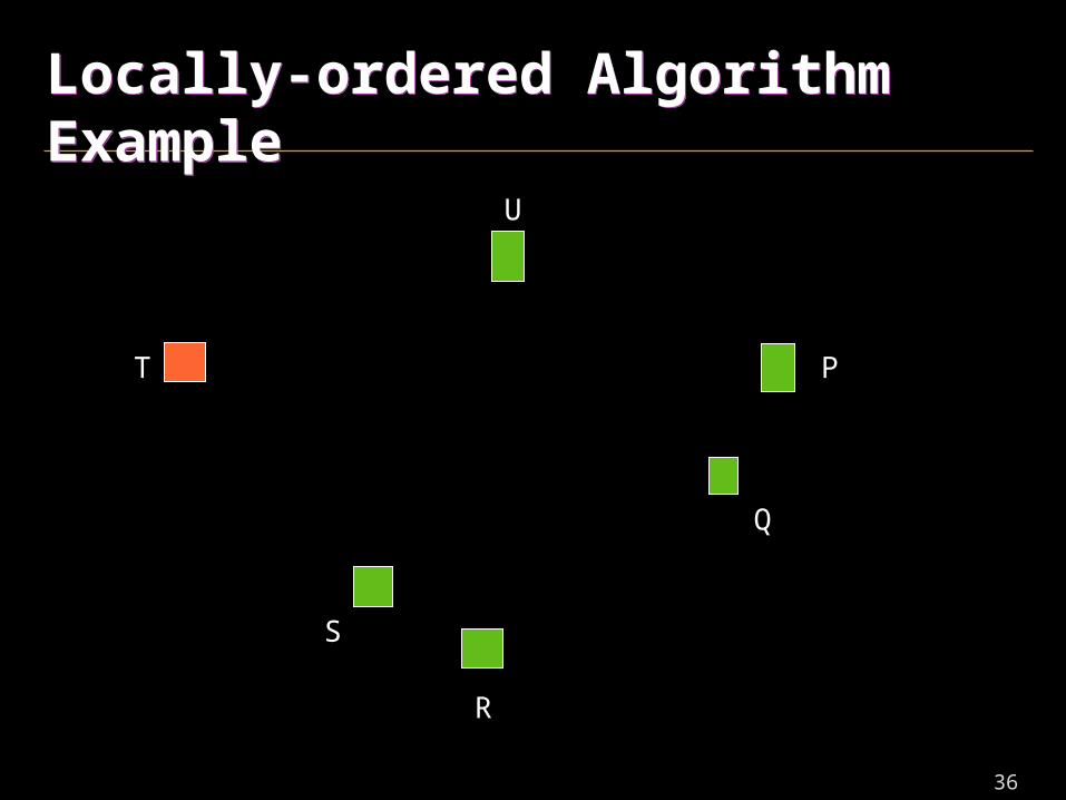
Locally-ordered Algorithm ExampleLocally-ordered Algorithm Example
P
U
Q
R
T
S
37
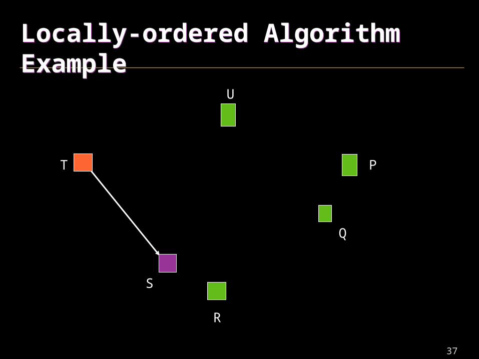
Locally-ordered Algorithm ExampleLocally-ordered Algorithm Example
P
U
Q
R
T
S
38
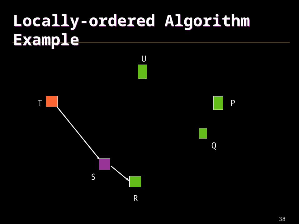
Locally-ordered Algorithm ExampleLocally-ordered Algorithm Example
P
U
Q
R
T
S
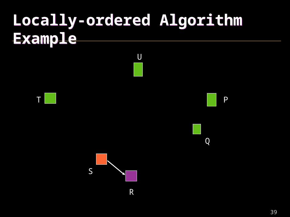
39
Locally-ordered Algorithm ExampleLocally-ordered Algorithm Example
P
U
Q
R
T
S

40
Locally-ordered Algorithm ExampleLocally-ordered Algorithm Example
P
U
Q
R
T
S
41
Locally-ordered Algorithm ExampleLocally-ordered Algorithm Example
P
U
Q
RS
T

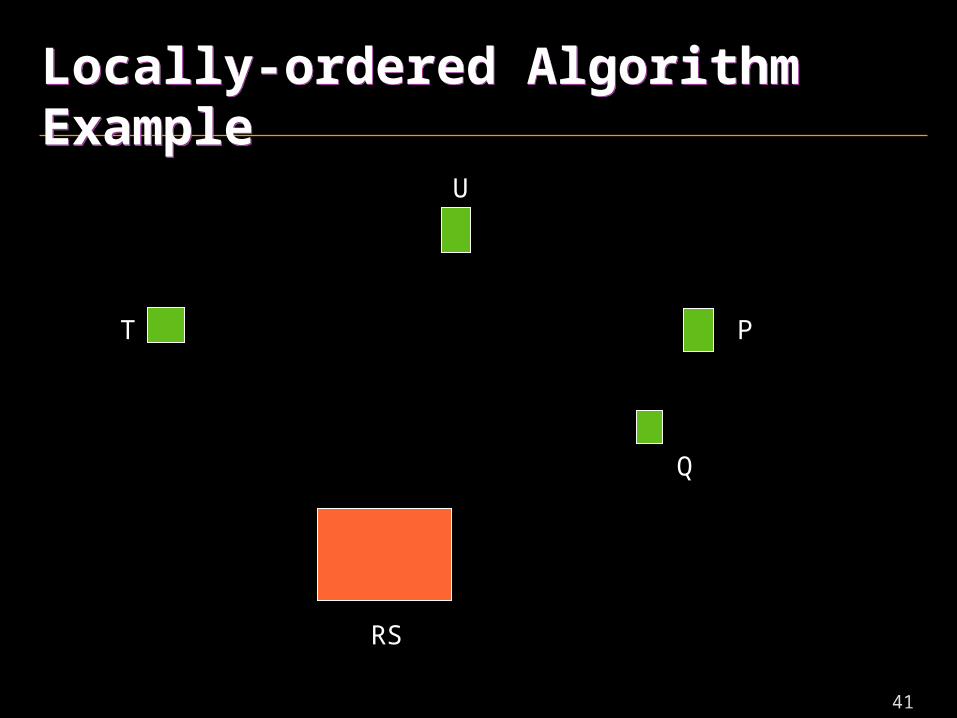
42
Locally-ordered Algorithm ExampleLocally-ordered Algorithm Example
P
U
Q
RS
T
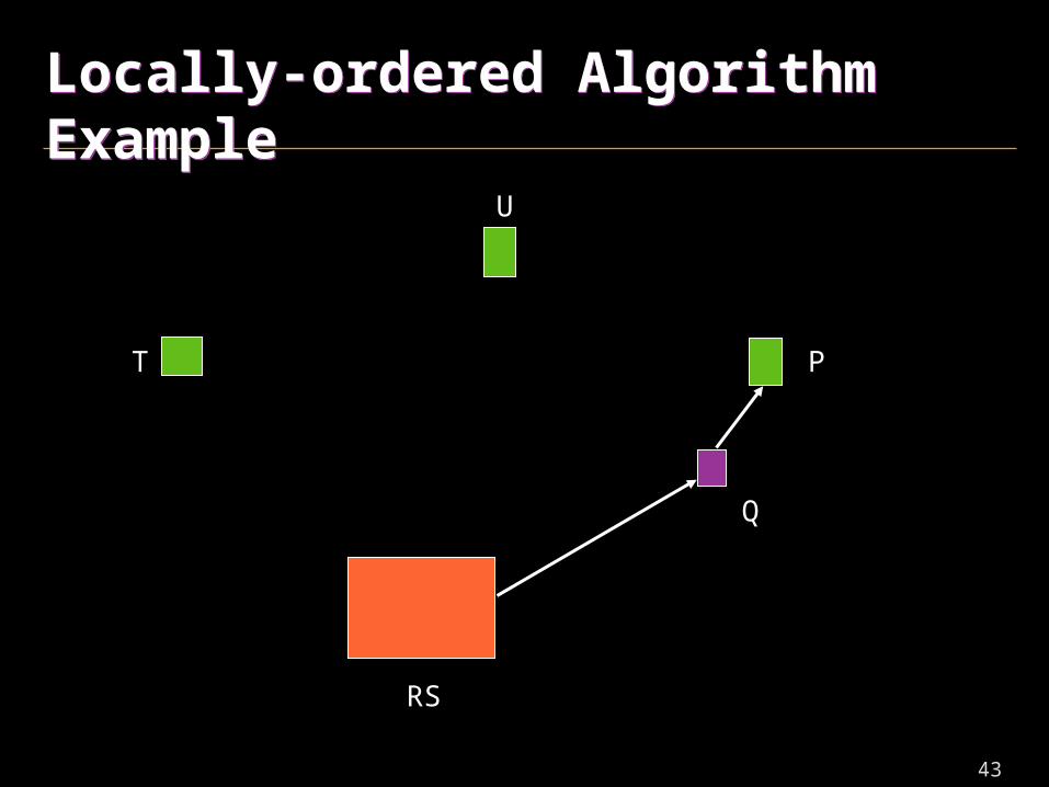
43
Locally-ordered Algorithm ExampleLocally-ordered Algorithm Example
P
U
Q
RS
T

44
Locally-ordered Algorithm ExampleLocally-ordered Algorithm Example
P
U
Q
RS
T
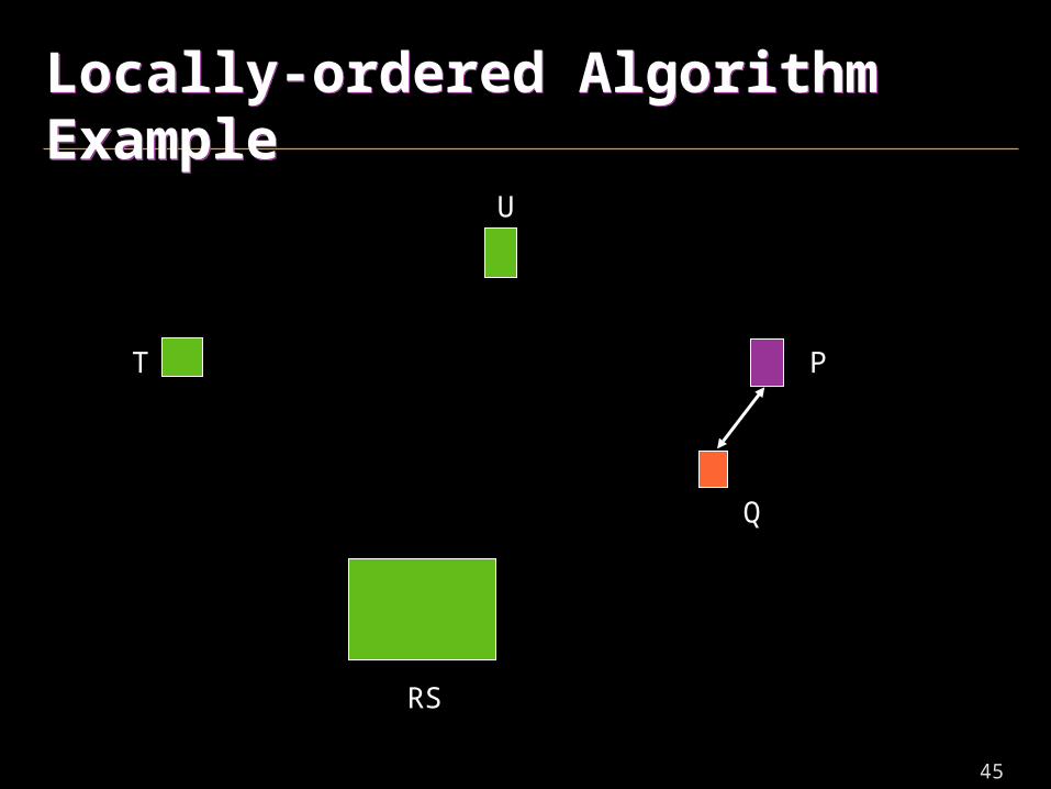
45
Locally-ordered Algorithm ExampleLocally-ordered Algorithm Example
P
U
Q
RS
T
46
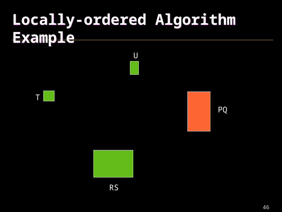
Locally-ordered Algorithm ExampleLocally-ordered Algorithm Example
PQ
U
RS
T
47
Locally-ordered AlgorithmLocally-ordered Algorithm
• Roughly 2x faster than heap-based algorithm
– Eliminates heap
– Better memory locality
– Easier to parallelize
– But d(A,B) must be non-decreasing
48
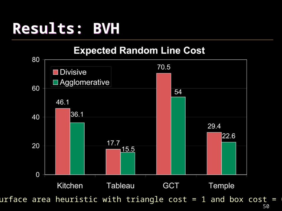
Results: BVHResults: BVH
• BVH – Binary tree of axis-aligned bounding boxes
• Divisive [from Wald 07]
– Evaluate 16 candidate splits along longest axis per step
– Surface area heuristic used to select best one
• Agglomerative
– d(A,B) = surface area of bounding box of A+B
• Used Java 1.6JVM on 3GHz Core2 with 4 cores
– No SIMD optimizations, packets tracing, etc.
49
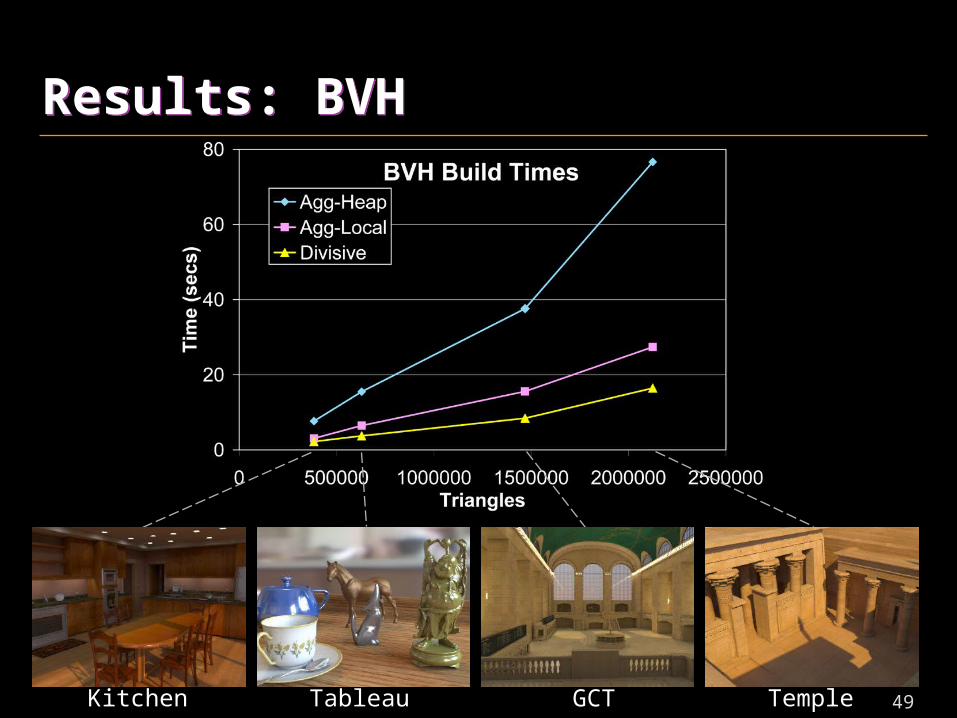
Results: BVHResults: BVH
Kitchen Tableau GCT Temple
50
Results: BVHResults: BVH
Surface area heuristic with triangle cost = 1 and box cost = 0.5
51
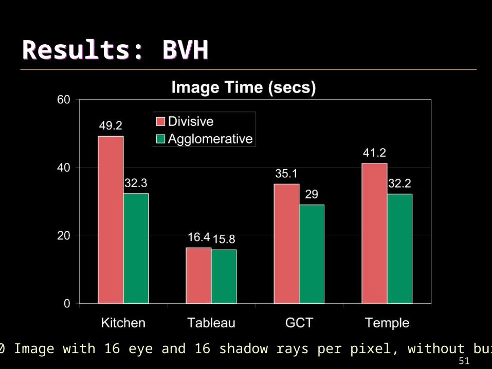
Results: BVHResults: BVH
1280x960 Image with 16 eye and 16 shadow rays per pixel, without build time
52
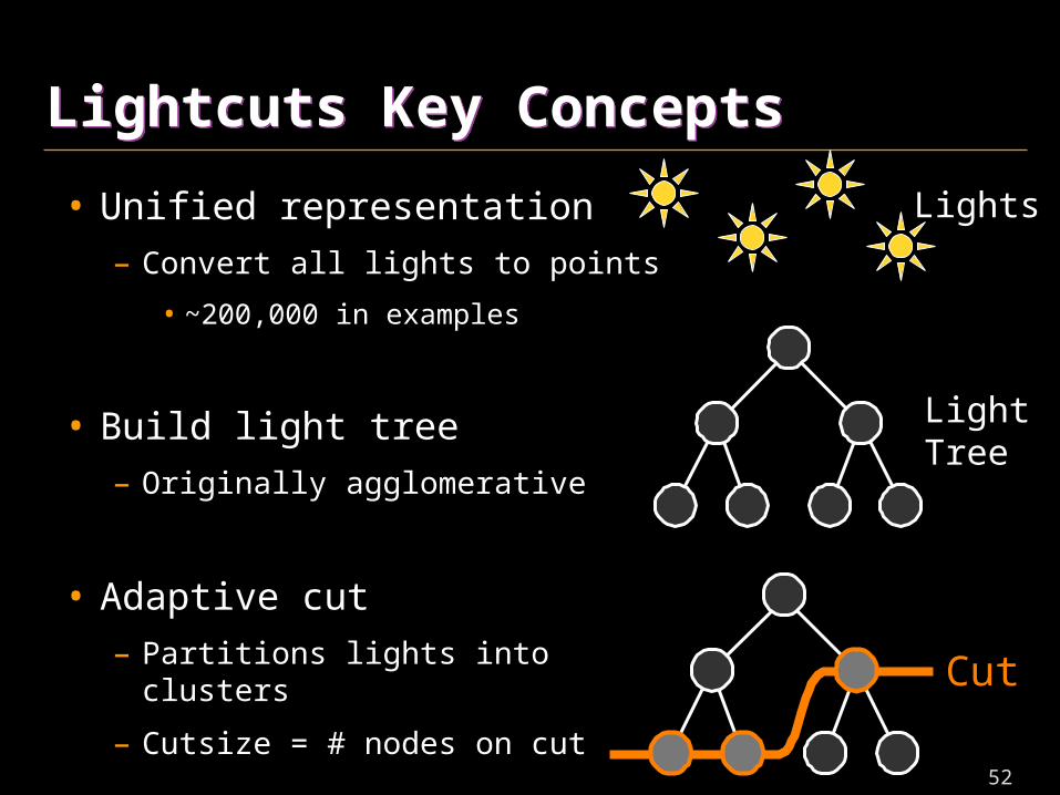
Lightcuts Key ConceptsLightcuts Key Concepts
• Unified representation
– Convert all lights to points
• ~200,000 in examples
• Build light tree
– Originally agglomerative
• Adaptive cut
– Partitions lights into clusters
– Cutsize = # nodes on cut
Cut
LightTree
Lights
53
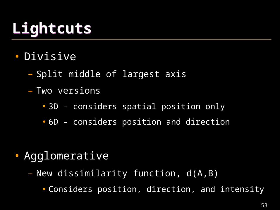
LightcutsLightcuts
• Divisive
– Split middle of largest axis
– Two versions
• 3D – considers spatial position only
• 6D – considers position and direction
• Agglomerative
– New dissimilarity function, d(A,B)
• Considers position, direction, and intensity
54
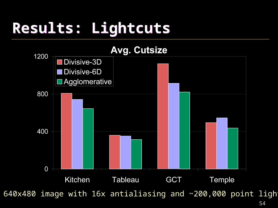
Results: LightcutsResults: Lightcuts
640x480 image with 16x antialiasing and ~200,000 point lights
55
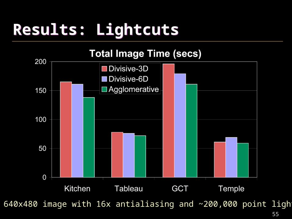
Results: LightcutsResults: Lightcuts
640x480 image with 16x antialiasing and ~200,000 point lights
56
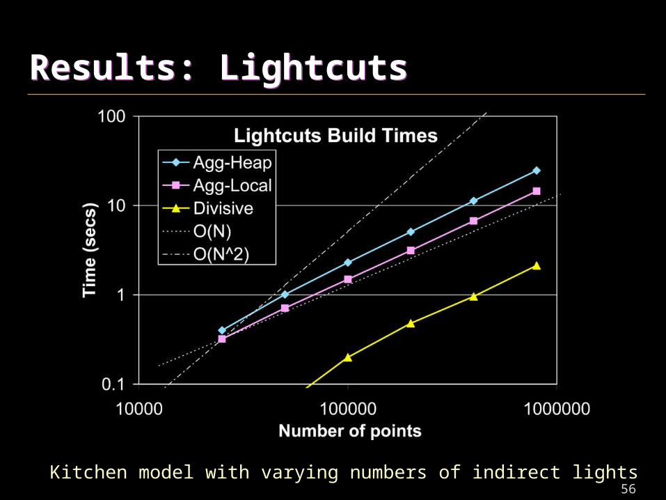
Results: LightcutsResults: Lightcuts
Kitchen model with varying numbers of indirect lights
57
ConclusionsConclusions
• Agglomerative clustering is a viable alternative
– Two novel fast construction algorithms
• Heap-based algorithm
• Locally-ordered algorithm
– Tree quality is often superior to divisive
– Dissimilarity function d(A,B) is very flexible
• Future work
– Find more applications that can leverage this flexibility
58
AcknowledgementsAcknowledgements
• Modelers
– Jeremiah Fairbanks, Moreno Piccolotto, Veronica Sundstedt & Bristol Graphics Group,
• Support
– NSF, IBM, Intel, Microsoft