FAST ALGORITHMS FOR SOLVING PATH PROBLEMS

by

Robert Endre Tarjan

STAN-CS-79-734April 1979

COMPUTER SCIENCE DEPARTMENTSchool of Humanities and Sciences

STANFORD UNIVERSITY

Fast Algorithms for Solving Path Problems

Robert Endre Tarjan*J

Computer Science DepartmentStanford University

Stanford, California 94305

April, 1979

Abstract.

Let G = (V,E) be a directed graph with a distinguished source vertex s .

The single-source path expression problem is to find, for each vertex v ,

a regular expression P(s,v) which represents the set of all paths in G

from s to v . A solution to this problem can be used to solve shortest

path problems, solve sparse systems of linear equations, and carry out

global flow analysis [30]. We describe a method to compute

path expressions by dividing G into components, computing path expressions

on the components by Gaussian elimination, and combining the solutions.

This method requires O(m a(m,n)) time on a reducible flow graph, where

n is the number of vertices in G , m is the number of edges in G J and

CI is a functional inverse of Ackermann's function. The method makes use

of an algorithm for evaluating functions defined on paths in trees [9,29].

e A simplified version of the algorithm, which runs in O(m log n) time on

reducible flow graphs, is quite easy to implement and efficient in practice.

CR Categories: 4.12, 4.34, 5.14, 5.22, 5.25, 5.32.

Keywords: Ackermann's function, code optimization, compiling, dominators,Gaussian elimination, global flow analysis, graph algorithm,linear algebra, path compression, path expression, path problem,path sequence, reducible flow graph, regular expression,shortest path, sparse matrix.

f* This research was partially supported by the National Science Foundationunder grant MCS75-22870-~02, by the Office of Naval Research undercontracts ~~044-402 and NOOOl4-76-C-0688, by the IBM Corporation, andby a Guggenheim Fellowship. Reproduction in whole or in part is permittedfor any purpose of the United States government.

1

1. Introduction.

The techniques of Gaussian and Gauss-Jordan elimination, originally

devised to solve systems of equations over the real numbers, have been

repeatedly rediscovered and applied to other problems. These include shortest

path problems [6,10,16], path-finding problems [4], global flow analysis

[2,12,13,23], and conversion of finite automata to regular expressions [18].

The most fundamental of these problems is the

expression problem: Given a graph G = (V,E)

source vertex s , find a regular expression

which represents all paths from s to v in

(single source) path

and a distinguished

p(s,v> for each vertex v

G . By reinterpreting

the U, l , and * operations used to construct regular expressions,

we can use a solution to the single-source path expression problem to

solve other kinds of path problems, including those mentioned above [30].

We thus obtain a general-purpose algorithm for solving any path problem

on a given graph.

This paper describes a decomposition method for computing path

expressions. The method divides the graph G into components based

upon the dominator tree of G , computes a path expression for each-

component by Gaussian elimination, and combines the solutions using

an algorithm for evaluating functions defined on trees [ 9,291. The

algorithm requires O(m a(m,n)) time plus time to compute path expressions

within the components, where n is the nwnber of vertices in G,

m is the number of edges in G , and a is a functional inverse of

Ackermann's function. If G is a reducible flow graph, each component

of G is a single vertex, and the method requires O(m a(m,n)) time

total. Although the method is rather complicated, a simplified version,

which runs in O(m log n) time, is quite easy to program and efficient

in practice.

The paper contains seven sections. Section 2 reviews the properties

of regular expressions used in the following sections. Section 3

reviews standard methods of numerical linear algebra and describes

their application to the path expression problem. This section introduces

the notion of a path sequence for a graph G and shows how, given a

path sequence, one can solve the single-source path expression problem

for any source in time proportional to the length of the path sequence.

Section 4 presents an O(m a(m,n)) -time algorithm for solving a single-

source path problem on a reducible flow graph if the source is the start

vertex of the graph. Section 5 extends the algorithm so that it

computes path sequences for reducible flow graphs. Section 6 generalizes

the method to non-reducible graphs. Section 7 discusses applications

and suggests further research topics. The appendix contains the basic

graph-theoretic terminology used in the paper, An earlier and much

different version of this paper appeared as a Stanford technical report [27].

2. Reaular Expressions and Path Expressions.

Let C be a finite alphabet containing neither "A" nor " #".

A regular expression over C is any expression built by applying the

following rules.

(1 1a ” A ” and ” F ” are atomic regular expressions; for any acz I

'1 a I? is an atomic regular expression.

w If Rl and R2

are regular expressions, -then (R1UR2) I

oyR2, 3 alei ml)* are campound regular expressions.

In a regular expression, A denotes the empty string, $ denotes

the empty set, u denotes set union, l denotes concatenation, and

* denotes reflexive, f*transitive closure under concatenation. Thus

each regular expression R over C represents a set c(R) of strings

over c defined as follows:

(24 a(A) = (A) ; o(d) = fi ; u(a) = (a) for aeC .

c(R*) =#

u mk , where c(R)' = {A) and a( = a(I$+c(R) .k=O

f* Note that each of the symbols A , fi y U , l , * stands in the text both

for the symbol itself and for a string, set, or operation. We shall

allow the context to resolve this ambiguity. Also, we shall freely

omit parentheses frcxn regular expressions when the meaning is clear;

we assume the standard operator precedence: * over l over U .

4

The reverse Rr of a regular expression R is defined by

(3 )a hr =A ; f=jb ; ar=a for sex.

(3b) (R+R~)'~ = RiuR; ; . .

(Rl'R2)' = <.Rjf ;

*rCR > r*1=1.0 >

Two regular expressions RI and R, are equivalent if a(5)

= c(R2) .

A regular expression R is simple if R = fl or

as a subexpression. We can transform any regular

equivalent simple regular expression by repeating

R does not contain $

expression R into an

the following

transformations until none is applicable: (i) replace any subexpression

of the form j$Rl or Rl*$ by fi ; (ii) replace any subexpression of

the form $+Rl or Rl+$ by Rl ; (iii) replace any subexpression

of the form $* by A.

A regular expression R is non-redundant if R represents every

string in a(R) uniquely. We can make this definition precise as

follows:

(4 )a Ar P ,, and a for each sex are non-redundant.

. P+w Let % and R2 be non-redundant.

Y R2 is non-redundant if c(Rl)nc(R2) = p .

Rl*R2 is non-redundant if each WE c(RlaR2) is uniquely

decomposable into w = wlw2 with wle a(l$) and

w2 E O(R2) l

5

*%

is non-redundant if each WE a(R*) is uniquely decomposable

into w = w w/

1 2*'*wk with wie c(R1) for 1 < i < k .a -

Note that if R* is non-redundant, Ai a) l

Let G = (V,E) be a directed graph. Any path in G is a sequence

of edges, which we can regard as a string over E . A path expression P

of w??e(VYW) is a simple regular expression over E such that every

string in o(P) is a path fram v to w . Every subexpression of a

path expression is a path expression, whose type can be determined as

follows.

(5) Let P be a path expression of type (v,w) .

If P = P1UP2 , then Pl and P2 are path expressions of

wee (v) l

If P = Pl'P2 , then there must be a unique vertex u such

that P, is a path expression of type (v,u) and P2

is a path expression of type (u,w1 l

If P = PI, then v = w and Pl is a path expression of

type (v,w) = (v,v) l

It is easy to verify (4) using the fact that P is simple. Note that

A is a path expression of type (v,v) for any v .

In describing algorithms to compute path expressions we shall assume

that each u , l ,and * operation requires constant time. If we

represent the computed path expressions by a directed acyclic graph as

described by Aho and Ullman [2, pp. 418-4261, this is a reasonable

assumption.

6

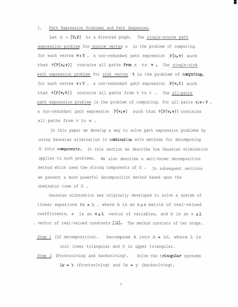
3. Path Expression Problems and Path Sequences.

Let G = (V,E) b e a directed graph. The single-source path

expression problem for source vertex s is the problem of computing,

for each vertex veV , a non-redundant path expression P(s,v) such

that c(P(s,v)) contains all paths frm s to v. The single-sink

path expression problem for sink vertex t is the problem of c~puting,

for each vertex veV , a non-redundant path expression P(v,t) such

that o(P(v,t)) contains all paths from v to t . The all-pairs

path expression problem is the problem of computing, for all pairs v,weV ,

a non-redundant path expression p(v,w> such that a(P(v,w)) contains

all paths from v to w .

In this paper we develop a way to solve path expression problems by

using Gaussian elimination in combination with methods for decomposing

G into components. In this section we describe how Gaussian elimination

applies to such problems. We also describe a well-known decomposition

method which uses the strong components of G . In subsequent sections

we present a more powerful decomposition method based upon the

dominator tree of G .

Gaussian elimination was originally developed to solve a system of

linear equations Ax = b , where A is an nxn matrix of real-valued

coefficients, x is an nX1 vector of variables, and b is an n xl

. vector of real-valued constants [lo-]. The method consists of two steps.

Step 1 (LU decomposition). Decompose A into A = LU, where L is

unit lower triangular and U is upper triangular.

Step 2 (Frontsolving and backsolving). Solve the triangular systems

w= 5 (frontsolving) and Ux = y (backsolving).

7

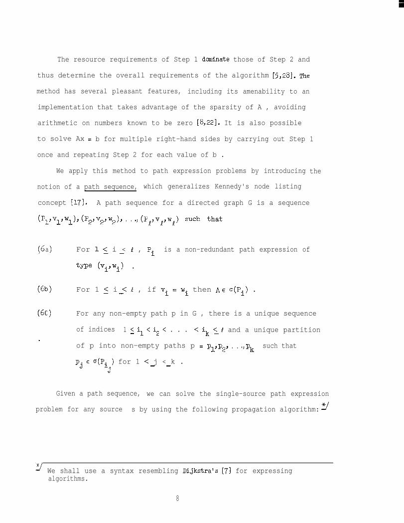
The resource requirements of Step 1 dominate those of Step 2 and

thus determine the overall requirements of the algorithm [5,28]. The

method has several pleasant features, including its amenability to an

implementation that takes advantage of the sparsity of A , avoiding

arithmetic on numbers known to be zero [8,22]. It is also possible

to solve Ax = b for multiple right-hand sides by carrying out Step

once and repeating Step 2 for each value of b .

1

We apply this method to path expression problems by introducing the

notion of a path sequence, which generalizes Kennedy's node listing

concept [17]. A path sequence for a directed graph G is a sequence

(pl’vpl~~ (P2,v2~w2)~ . . ., (Pppp) such that

(6 1a For l< i < I , Pi- - is a non-redundant path expression of

type (viYwi) l

(6W For 1 < i < I , if vi = wi then AE: "(Pi) .- -

(6 >C

-

For any non-empty path p in G , there is a unique sequence

of indices 1 < il < i2 < . . . < ik < I and a unique partition-

of p into non-empty paths p = pl,p2, . . ., pk such that

pj E c(Pi ) for 1 < j < k .- -j

Given a path sequence, we can solve the single-source path expression

problem for any source -/*s by using the following propagation algorithm:

*J We shall use a syntax resembling Dijkstra's [7] for expressing

algorithms.

8

procedure SOLVE;

begin

initialize: WY s> := A; for~/eV-(s} g P(S,V) := fi 9

loop: for i := 1 until & doNW -

if v. = w-1 i 3 'CsYvi) := [P(S,Vi).Pil

j-j vi f wi 4 P(S,Wi) := Fp(‘Ywi) U ~p(sYv~)‘p~ll ~ ~

end SOLVE;-

In this and subsequent algorithms, the square brackets denote the

following simplification procedure. This procedure, when applied

recursively, produces regular expressions that are not only simple but aiLso

*contain no subexpressions of the form AoR, , R,eA , or A .

regular

ifrye

II

Ll

expression procedure

R = R1uR;! - 1 =+if R

R = Rl*R2 + if (Rl =-

R = R" 3i.f (Rl = $)-

[RI;

fl 4 R2 n R2 = p -) Rls

8) or (R2 = $) + @ 1 Rl = h --) R2 a R2 = A 4 Rl 2

or (Rl = A) -+ A fi fi*- --'

-Lemma 1. Let Ppyy), (p2,v2,w2), . ..) (pp vp WI) be a path sequence

for G and let v be any vertex. After i iterations of the loop in

SOLVE, P(s,v) is a non-redundant path expression representing exactly A

(if s = v ) and all non-empty paths p from s to v for which there

is a sequence of indices 1 5 il < i2 < . . . < ik < i and a partition of

P into P = PlJP2J .*a, pk such that pj E c(Pi ) for 1 < j < k .- -j

Proof. Straightforward by induction on i . 0

Theorem 1. Let (P,Yv,Yw,)Y (P,tv,,w,), l . ., (Ppp’wL) be a path sequence

for G and let v be any vertex. After execution of SOLVE, P(s,v) is

a non-redundant path expression representing all paths from s to v.

SOLVE is a generalization of the frontsolving-backsolving step in

@XlsSian elimination; its running time is O(n+l) . To solve a single-

source path expression problem on a graph G , we construct a path

sequence and apply SOLVE once. To solve an all-pairs path expression

problem, we construct a path sequence and apply SOLVE n times, once

for each possible source. To solve a single-sink path expression problem,

we employ the following theorem to construct a path sequence for Gr ,

and then we solve the corresponding single-source problem on Gr .

Theorem 2. Let (Ply~lywl)y (P2yv2yw2)y ..a, (Pppl) be a path sequence

for a graph G . men (P~ywl~vl)~~ l l t (P~,w~~v~)~ (P~,wl,-y) is a path

sequence for Gr .

Proof. Immediate. B

By Theorem 2ato compute a path

it is no harder to compute a path sequence for Gr than

sequence for G .

We can construct a path sequence for an arbitrary graph by using a

method analogous to Step 1 of Gaussian elimination. The method is similar

to KLeene's algorithm for converting a finite automaton into a regular

expression [18], except that Kleene uses Gauss-Jordan elimination. Let

G = (V,E) be a directed graph whose vertices are nwnbered fram 1 to n

and identified by number. The following procedure computes a set of path

expressions which when properly ordered gives a path sequence.

10

procedure ELIMINATE;

begin

initialize: for v := 1 until n do for w- := 1 until n do P(v,w) :=- NV

for each eeE do P(';;;e),t(e)) := [P(h(e),t(e))Ue] od;

j6 od od*NV n.u'

loop:

- - -

for v := 1 until n do-

P(vY 4 := &,v)*l ;

-

for each u > v such that P(u,v) # $ doNIN- ryvwrvvw -

phv) : = [P(u,v)*P(v,v)l;

fororW>V~~P(V,W) f @do-

p(u, w) := [P(u,w) u [P(u,v)~P(v,w)l] od od-Twend ELIMINATE;-

Lemma 2. After the v-th iteration of the loop in ELlNU!iATE, the following

statements are true.

(i) P(u,w) for u > w and w < v is a non-redundant path expression

representing exactly the paths from u to w which contain no

intermediate vertex larger than w .

(ii) P(u,w) for u < w or w > v is a non-redundant path expression

representing exactly the non-empty paths from u to w all of

whose intermediate vertices are smaller than min{u,v+lj .

-Proof. Straightforward by induction on v . Cl

ll

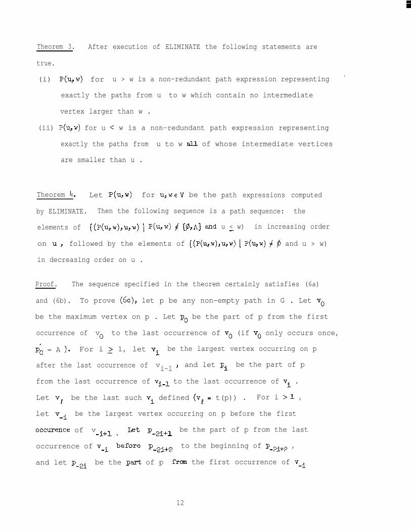
Theorem 3. After execution of ELIMINATE the following statements are

true.

(i) P(u,w) for u > w is a non-redundant path expression representing '

exactly the paths from u to w which contain no intermediate

vertex larger than w .

(ii) P(u,w) for u < w is a non-redundant path expression representing

exactly the paths from u to w all. of whose intermediate vertices

are smaller than u .

Theorem 4. Let P(u,w) for u,weV be the

by ELIMINATE. Then the following sequence is

elements of ((P~u,w),u,w) \ P(u,w) i %A] and

path expressions computed

a path sequence: the

u < w) in increasing order-

on u, followed by the elements of ~(P(u,w),u,w) \ P(u,w) # fi and u > w)

in decreasing order on u .

Proof. The sequence specified in the theorem certainly satisfies (6a)

and (6b). To prove (6c), let p be any non-empty path in G . Let v.

be the maximum vertex on p . Let p. be the part of p from the first

occurrence of vo to the last occurrence of v. (if v. only occurs once,a

PO = A )* For i > 1, let vi be the largest vertex occurring on p-

after the last occurrence of vi-l ' and let pi be the part of p

from the last occurrence of vi-1 to the last occurrence of vi .

Let v1 be the last such vi defined (va = t(p)) . For i >l ,

let vWi be the largest vertex occurring on p before the first

occurence of v-i+l l Let p-2i+l be the part of p from the last

occurrence of vvi before P_2i+2 to the beginning of p-2i+2 ,

and let p-2i be the psrt of p from the first occurrence of vmi

12

to the beginning of p-2i+l . Let vWk be the last

such v-i defined (vWk = h(p)) . Then

P = P,2kYP_2k+lY"'JP_l'PO'P1'".JPp with P-2-i' 0(p(V-i9v-i)) for

O<i<k,- - '-2i+l E ~(P(v-~,v-~+~)) for 1 5 i 5 k , and

pie ~(P(v~-~,v~)) for 15 i 5 1 . Ignoring empty paths pi y we get

a partition of p which satisfies (6b). It is straightforward but

tedious to show that this partition is unique. 0

ELIMINATE thus gives us a way to construct path sequences. The resource

requirements of the method depend in a complicated way upon the sparsity

of G . By rearranging the computation in the loop of ELIMINATE and

using appropriate data structures we can implement ELIMINATE to run in

0 1 + 5 1 EPbYv) # lb 1 u > v] I* Icp(v,w> # p \ w > v’) \ time and O(m>v= 1

storage space, where 1 is the length of the computed path sequence

[ 5,281. (By only storing P(u,w) for pairs u, w such that eventually

pb,w> f p Y we can avoid spending O(n2) time in initialization.)

For dense graphs the time bound is 3O(n +m) and the space bound

is O(n2) . For sparse graphs, the resource requirements depend upon

the vertex nwnbering chosen. Numerical analysts have devoted much

. effort to finding good numbering schemes, both for arbitrary sparse

graphs and for graphs with special. structure t&8,22,28].

All their techniques except off-diagonal pivoting [ll] apply to the

computation of path sequences.

In order to improve the efficiency of this method, we shall combine

it with two decomposition techniques. The idea is to break the problem

13

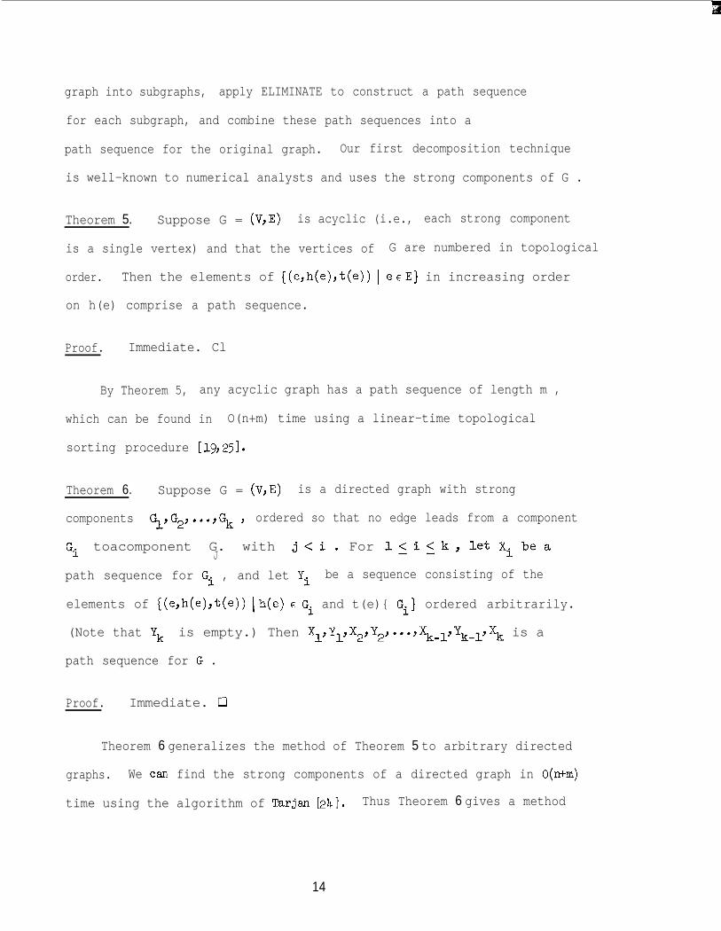
graph into subgraphs, apply ELIMINATE to construct a path sequence

for each subgraph, and combine these path sequences into a

path sequence for the original graph. Our first decomposition technique

is well-known to numerical analysts and uses the strong components of G .

Theorem 5. Suppose G = (V,E) is acyclic (i.e., each strong component

is a single vertex) and that the vertices of G are numbered in topological

order. Then the elements of {(e,h(e),t(e)) \ eeE} in increasing order

on h(e) comprise a path sequence.

Proof. Immediate. Cl

By Theorem 5, any acyclic graph has a path sequence of length m ,

which can be found in O(n+m) time using a linear-time topological

sorting procedure [lg,25].

Theorem 6. Suppose G = (V,E) is a directed graph with strong

components Gl,G2,-,Gk Y ordered so that no edge leads from a component

Gi toacomponent G. with j<i. For l~iLk,let Xi beaJ

path sequence for Gi , and let Yi be a sequence consisting of the

elements of {(e,h(e),t(e)) \h(e) e Gi and t(e){ Gi] ordered arbitrarily.

(Note that Yk is empty.) Then Xl,Yl,X2JY2,...,XklyYk-l,Xk is a

path sequence for G .

Proof. Immediate. 0

Theorem 6 generalizes the method of Theorem 5 to arbitrary directed

graphs. We can find the strong components of a directed graph in O(n+m)

time using the algorithm of Tarjan [24]. Thus Theorem 6 gives a method

14

for finding a path sequence in O(n+m) time plus the time to find

path sequences for the strong components. The length of the sequence

is O(m) plus the total length of the strong components' sequences.

15

4. Computing Path Expressions for Reducible Flow Graphs.

Although decomposition using strong components is efficient and

useful in practice, many problem graphs have one or ,only a few strong

components. In the remaining sections of this paper we develop a more

powerful decmposition technique based upon dominators. We begin by

considering reducible flow graphs. A flow graph G = (V,E,r) is a

directed graph with a distinguished start vertex r such that every

vertex in G is reachable from r . By Theorem 6 we need only consider

strongly connected graphs, SO this reachability condition is no restriction.

A reducible flow graph G = (V,E,r) is a flow graph that can be

reduced to the graph consisting of the single vertex r and no edges

by means of the following transformations:

Tl(remove a loop): If e is an edge such that h(e) = t(e) , delete

edge e .

T2(remove a vertex): If w#r is a vertex such that all-edges e

with t(e) = w have h(e) = v for some vertex v , contract w

into v by deleting w and all edges entering w , and converting

=lY edge e with h(e) = w into an edge e' with h(e') = v-

and t(e') = t(e) .

This definition is due to Hecht and UUman [lb]; there are many other

equivalent definitions of reducible flow graphs [12,14,15,2~], Intuitively

a flow graph is reducible if every cycle has a single entry from the

start vertex. These graphs play an important role in global flow analysis,

because the control flow of a reasonably well-structured program can be

modelled by a reducible flow graph [3,20].

16

As the reduction by Tl and T2 takes place, each vertex in the

reduced graph represents a subgraph of the original graph, called a

region, and each edge in the reduced graph represents an edge in the

original graph. We define this notion formally as follows.

(7 1a Each vertex and edge in the original graph represents itself.

(7b) If Tl is applied to delete an edge e , then vertex h(e) = t(e)

in the reduced graph represents the union of what h(e) and e

represent.

(7 >C If T2is applied to contract vertex w into vertex v , then

V in the reduced graph represents the union of what v , w ,

and all the deleted edges e with h(e) = v , t(e) = w

represent. Any new edge e' represents what the corresponding

old edge e represents.

It is not hard to show that each region is indeed a subgraph of G

and that the regions corresponding to the vertices of any reduced graph

are vertex-disjoint [31]. Furthermore every region I has a unique

header vertex v such that any edge e with h(e)#I , t(e) E I hasa

t(e) = v [31]. The header is the unique vertex in the region which has

not yet been contracted into another vertex. When the reduction is

complete, r represents a region comprising the entire graph G .

If a flow graph is reducible, there is a reduction order vl,~2,.,.,~n-1,~n=r

of the vertices such that the graph can be reduced to r in the following

way WI : For i from 1 to n-l , we apply Tl to delete all loops

at v.1 ; then we apply T2

to contract vi into another vertex v3

with

17

j>i. After deleting all vertices except vn = r , we apply Tl to

delete all loops at r . This way of carrying out the reduction has the

following property. If we regard the repeated application of Tl at a

vertex vi followed by the application of- T2 to delete vi as a single

step, then between any two steps the entry vertex of any region has no

edges entering it from within the region.

We shall assume henceforth that the vertices of G are numbered

from 1 to n in a reduction order and identified by number. We shall

also assume that header(v) for v # r is the vertex into which v is

eventually contracted, that cycle(v) for any vertex v is the set of

edges in G represented by edges deleted when applying Tl to delete loops

at v , and that noncycle for v # r is the set of edges in G

represented by edges deleted when applying T2 to delete v . The following

lemma states some basic properties of header , cycle , and noncycle.

Lexmna 3. Suppose G is a reducible flow graph whose vertices are

numbered in a reduction order. Let v be

any edge. Then

any vertex and let e be

( >i if v#r, header(v) > v ;a

( >ii either h(e) = header(t(e)) or h(e) 5 t(e) ;

(iii) if eecycle(t(e)) then headeri(h(e)) = t(e) for some i > O ; a n d_

( >iv . if eenoncycle(t(e)) then headeri(h(e)) # t(e) for all i>O

but headeri(h(e)) = header@(e)) for some i > 0 .

Proof. Straightforward. 0

18

3

The algorithm of Tarjan [26] computes a reduction order and

associated arrays header , cycle , and noncycle in ob ebn>>

time. Using this information we can solve the single-source path

expression problem whose source vertex is r . The algorithm

resembles the methods of Ullman [31] and Graham and Wegman [12] for

solving "forward" data flow problems; we discuss this resemblance at

the end of the section.

The algorithm computes path expressions as the reduction proceeds,

using a data structure representing the current regions. The data

structure consists of a forest whose vertices are the vertices of G

and whose edges are the pairs (header(v),v) such that v has been

contracted into header(v) . Thus this header forest consists of one

tree per region; the tree representing a region contains exactly the

vertices in the region and has the header of the region as its root.

With every vertex v in the forest is associated a non-redundant path

expression R(v) . The algorithm manipulates the forest by means of

four operations:

INITIALIZE(v): Form a tree with one vertex v and associated path

expression R(v) := A .

UPDATE(v,R): If v is a root, assign R(v) := R ,

. LINK(v,w): If v and w are roots, combine the trees with

roots v and w by making v the parent of w .

EVAL(v): If r = v. -) vl -, v2 + . . . --) vk = v is the tree

path fram the root r of the tree containing v

to v, return a non-redundant path expression

equivalent to R(vo) . R(vl) . . . . . R(vk) .

19

The algorithm maintains the following invariant: If I is a region and

V is a vertex in I , then EVAI, represents exactly all paths in I

from the header of I to v .

procedure REDUCE;

begin

initialize: for each WV do INITIALIZE(v) od-;- - -

loop: for v := 1 until n-l do

- :=pxp; -P

for each e enoncycle(v) z P := [PU [EVAL(h(e)).e]] od;NW-

for each ee cycle(v) _do Q := [Qu[EVAL(h(e))~e]] od;Nyv- -

finalize:

-UPDATE(v,[P+Q*]]);

LINK(header(v),v) s;

P(r,r) := p;

> := [P(r,rfor each ee cycle(r) do P(r,ra - -

p(r, r> := [P(r,r)*];

> U [Wfi(h(eX41 od;

for v := 1 until n-l do P(r,v) := [P(r,r)4ML(v)] od- -

end REDUCE;NVV

-

Lemma 4. After the v-th iteration of the loop in REDUCE, ~Uu)

for any vertex u represents exactly all paths in the current region I

containing u from the header of I to u .

Proof. By induction on v . The lemma is certainly true before the

first iteration of the loop. Suppose the lemma is true before the v-th

iteration of the loop. Let I1 be the current region containing v and

20

let I3 be the current region containing header(v) . Let I2 be the

region containing v afterTl is applied to eliminate all loops at v .

Let I4 be the region containing v after T2 is applied to contract

v into header(v) ; i.e., after the v-th iteration of the loop.

I2 consists of I1

and the edges in cycle(v) . I4 consists of

I2 J I3 Y and the edges in noncycle ; the header of I4 is the

header of I3 l

I1contains no edges entering v . It follows from the induction

hypothesis that the value of Q after the v-th iteration is a non-redundant

path expression representing all paths fram v to v in I2 which do not

contain v as an intermediate vertex. Thus Q* represents all paths in

I2 from v to v . It also follows from the induction hypothesis that

the value of P after the v-th iteration is a non-redundant path expression

representing all paths in I4 from the header of I4 to v which do not

contain v as an intermediate vertex.

If u is a vertex in5 ,

then the paths in I4 fram the header

Of I4 to u are exactly the paths inI3

from the header of I3

to u . If u is a vertex in I2 , the paths in I4 from the header

of I4 to u are exactly the paths p partitionable intoa

P = P~YP~JP~ Y where ale o(P) Y ~2e a(Q*) Y and P3is a path in

I1fram the header of I1 to u . Thus adding edge (header(v),v)

to the forest and replacing the old value (A) of P(v) by [P.[Q*]]

guarantees that the lemma holds after the v-th iteration of the loop. a

21

Corollary 1. After execution of REDUCE, R(v) for any vertex v # r

is a non-redundant path expression representing exactly the set of

paths from header(v) to v all of whose intermediate vertices are

smaller than header(v) .

Proof. For any vertex v # r , let I4 be the region containing v

after the v-th iteration of the loop in REDUCE. Let R(v) be the path

expression computed for v during this iteration. By Lemma 4,

NV) is a non-redundant path expression representing all paths in

I4 from header(v) to v . Any path in G from header(v) to v

which leaves I4 must contain header(v) twice, since the only way

to enter I4 is through header(v) . 0

Theorem 7. Let v any vertex. After execution of REDUCE, p(r, v>

is a non-redundant path expression representing all paths from r to v.

Proof. Lemma 4 hold s after the last iteration of the loop in REDUCE.

A proof similar to that of Lemma 4 shows that P(r,r) as computed in

the final part of REDUCE is a non-redundant path expression representing

all paths from r to r in G l It follows from Lemma 4 that theacomputed value of P(r,r) for v # r is a non-redundant path expression

representing all paths from r to v in G . i3

Procedure REDUCE requires O(n+m) time plus time for n calls

on INITIALIZE, n-l calls on UPDATE, n-l calls on LINK, and m+n-1

calls on EVAL; thus the forest manipulation operations dminate the

running time of the algorithm. Tarjan [29] describes two ways to

implement the forest operations. The first is a simple method

22

called path compression which requires O(m log n) time. The second

is a sophisticated off-line method which by preprocessing the entire

sequence of EVAL

manipulation in

sequence of EVAL

presents another

and LINK operations is able to perform all the forest

O(m a(m,n)) time... (It is easy to precompute the

and LINK operations performed by REDUCE.) Farrow

O(m CX(m,n)) -time method called stratified path

[91

compression. This method has the advantage of being on-line, although

the proof of its time bound is very complicated.

By using either of the O(m a(m,n)) -time algorithms for forest

manipulation we obtain a moderately complicated O(m a(m,n)) -time

implementation of REDUCE. By using path compression we obtain an

O(m log n) -time implementation of REDUCE which is remarkably simple

and efficient. We favor the latter implementation for practical

applications.

Ullman's algorithm for forward data flow analysis [31] is essentially

identical to REDUCE except that it uses Z-3 trees to carry out the forest

operations. Its time bound is O(m log n) but it is more complicated

than our method using path compression. Graham and Wegman's algorithm [12]

is a version of REDUCE which uses no auxiliary data structure but carries

out a form of path compression on the original graph. Its time bound

is O(m log n) but it also is more complicated than our method using

path compression. Experimental comparisons between these methods would

be valuable.

23

5. Computing Path Sequences for Reducible Flow Graphs,

Some kinds of data flow analysis, such as the computation of live

variables [17], require that information be propagated backward rather

than forward through the control flow graph of the program. We can

carry out such backward data flow analysis by solving a single-source

path problem on the reverse of the control flow graph. Since reducibility

is not preserved by graph reversal, the algorithm of Section 5 is

inadequate for this purpose. In this section, we shall modify REDUCE

so that it computes a path sequence for any reducible flow graph. By

using such a path sequence and applying Theorem 6 if necessary, we can

solve single- and multi-source path problems on any flow graph which is-_

reducible or whose reverse is reducible, This provides an efficient way

to do backward data flow analysis.

In order to develop this algorithm, we need to examine the implementation

of the header forest operations. We shall describe a generic implementation

of which path compression [29] and stratified path compression [ g]

are special cases. We shall use this generic implementation in an

extension of REDUCE which computes path sequences.

- The generic implementation uses a compressed forest to represent the

header forest. With each vertex v3

of the compressed forest is

associated a path expression SW . The method maintains the following

invariants.

(8 >a For each tree T in the header forest, there is a corresponding

tree TC of the compressed forest which contains the same

vertices as T .

24

VW If VdW in a tree TCof the compressed forest, then

*v-*w in T . In particular, corresponding trees T and TC

have the same root.

(8 >C For any vertex v , let r = v. 3 vl + . . . + vk = v be the

path in the header forest from a root to v , and let

r = w +w d...-+W0 1 B

= v be the path in the compressed

forest from a root to v . Then R(vo) . R(vl) l . . . l R(vk)

and S(wo) l S(wl) l . . . l S(w& are equivalent non-redundant

path expressions.

The compressed forest is represented by an array ancestor such

that ancestor(v) is the parent of v in the campressed forest; if

ancestor(v) = 0 then v is a root. The following procedures implement

the forest operations.

INITIALIZE(v);

bz ancestor(v) := 0; S(v) := A er&;

procedure UPDATE(v,R);

a S(v) := R;

procedure LINK(v,w);

ancestor(w) := v;

25

w expression procedure EVAL(v);

begin

non-deterministically execute COMPRESS(u) for an

arbitrary sequence of vertices u;

let y)‘V~, . . ..vk be such that v = vk, ancestor(vi) = vim1 for

for l< i 5 k, and ancestor(vo) = 0;

EVAL :=ifk=O31\

llkf 0 3 s(vl) l s(v2) l . . . l S(Vk)

end EV'AL;-

procedure COMPRESS(u);-_

g ancestor(ancestor(u)) # 0 4

SW := S(ancestor(u)) . S(u);

ancestor(u) := ancestor(ancestor(u)) fi;-

It is evident that COMPRESS preserves (8a)-(8c); thus the procedures

above are a valid implementation of the header forest operations. The

following lemma is easy to prove using the results in Section 4.

fi

Lemma 5.2 If v is any vertex such that ancestor(v) # 0 , then S(v)

is a non-redundant path expression representing exactly the set of paths

from ancestor(v) to v all of whose intermediate vertices are smaller

than ancestor(v) .

EVAL is a non-deterministic procedure which is free to choose an

arbitrary sequence of vertices u on which to execute COMPRESS(u) .

We obtain a specific implementation by including a mechanism for making

this choice. Path compression uses the following version of EVAI.,.

26

3

expression procedure ENAL(

if ancestor(v) = 0 -) EVA.L := A

/I ancestor(v) # 0 -+ PATH~COMPREsS(v

procedure PATH-COMPRESS(v);

g ancestor(ancestor(v)) # 0 3

PATH-COMPRESS(ancestor(v));

s(v) := S(ancestor(v)) l S(v);

); EVAL := S(v

ancestor(v) := ancestor(mcestor(v)) fi;-

> fi.*-’

Stratified path compression uses a more complicated compression mechanism

which requires the maintenance of additional data structures [g].

The following version of REDUCE uses the generic implementation of

the header forest operations to compute a path sequence. Procedures

EVAL and COMPRESS are modified so that they add elements to the path

sequence as a side effect.

27

addl:

w REDUCE AND-SEQUENCE;

begin

initialize: for each WV do INITIALIZE(v) od;NW-' r-4-2 ,-=N

sequence := the empty sequence;

loop: for v := 1 until n-l do-

:= f!iii p;

-

P

for each eenoncycle(v) do P- - - := [PUEVAL AND SEQUENCE(e)]- - od;-

for each e E cycle(v) E Q :=- - [QUEVAL AND SEQUENCE(e)]- - od;

g[Q*l #A 4 add ([Q*],v,v) to sequence fi;-

mDATE(v, [P* [ Q*l I) ;

LINK(header(v),v) od;-

finalize: Q := j?j; --

for each eecycle(r) do Q--J - - := [QUEVAL AND SEQUENCE(e)]a - od-;

add2: E IQ*] # A 3 add ([Q*],r,r) to sequence 2;

for v :=- n-l by -1 until1 do add (S(v),ancestor(v),v) to sequence od- - -

end REDUCE AND SEQUENCE;- - -

procedure EVALJND-SEQWCE(e);

begin

non-deterministically execute COMPRESS AND SEQUENCE(u) for- -

an arbitrary sequence of vertices u;

let VOY VlJ . . ..vk be such that h(e) = vk, ancestor(vi) = vi 1 for

15 i 5 k, and ancestor(vo) = 0;

ifk=O- 4 EVAL AND SEQUENCE := e

Ilk+0 1 I4 EVAL AND SEQUENCE := S(v,)ee;

for i := k-l by -1 until 1 do- - -

add (EVALJND~SEQUENCE,vi,t(e)) to sequence;I

EVALJND-SEQUENCE := S(vi) ' EYALJND SEQUENCE od fiTw-end EJVAL AND SEQUENCE;- - -

28

procedure COMPRESS/D-SEQUENCE(u);

2 ancestor(ancestor(u)) # 0 -+

add (S(u),ancestor(u),u) to sequence;

SW := S(ancestor(u))43(u);

ancestor(u) := ancestor(ancestor(u)) g;

Theorem 8. The sequence computed by REDUCE-AND SEQUENCE is a path

sequence for G .

Proof. The

complicated.

add1 always

proof is similar

We shall assume

adds ([Q*.*],v,v)-_

to the proof of Theorem 4 but a little more

for purposes of the proof that statement

to sequence , whether or not [Q*l = A ;

similarly for statement add 2. This modification does not affect the

properties of sequence in which we are interested.

Lemma 5 and an inspection of REDUCE AND SEQUENCE show that the computed- -

sequence satisfies (6a) and (6b). To prove (6c), let p be an arbitrary

path in G . Let v. = h(p) . For i > 1 , let v- i be the first vertex

on P such that vi > v.1-l l

Let vk be the last vertex so defined

(vk is the largest vertex on p ). Let v~+~ = t(p) . Let p2k be the

a part of p from the first occurrence of vk to the last occurrence of vk .

Let '2k+l be the part of p following p2k . For 0 < i < k-l , let

p2i+l be the part of p from the last occurrence of vi before p2i+2

to the beginning of p2i+2 l Let P2i be the part of p from the first

occurrence of vi to the beginning of p2i+l . men P = PO'P1'"e'P2k+l ,

where p2i for 0 < i < k is a path from vi to v.a - 1 containing no

vertex greater than viYmd P2i+l for 0 < i < k is a path from v,- - 1

-ILo vi+l all of whose intermediate vertices are less than vi .

29

For O<i<k,- - P2iE '(Q*(Vi)) Y where Q(vi) for vi f r

is the value of Q computed during the vi -th iteration of the loop

in REDUCE-AND-SEQ;rJENCE, and Q(r) is the value of Q computed during

the final part of REDUCE-AND-SEQUENCE. In order to represent p as

in (6c), it remains for us to (i) partition each path p2i+l for

0 < i 5 k-l into a sequence of paths represented by triples appearing

in sequence between ([Q(vi)*I>Vi>Vi) ad ([Q(Vi+l)*I,Vi+l,Vi+1) Y

and (ii) partition p2k+l into a sequence of paths represented by

triples appearing in sequence after ( [Q(vk)*],vkyvk) .

Consider any path pQi+, for 0 < i < k-l . Let e, be the last- -

edge on

of v.1

loop in

'2i+l =

(0)p2i+l =

L.L’A I

this path-. Then t(ei) = vi+1 , and h(ei) is a descendant

in the compressed tree just after the vi -th iteration of the

REDUCE-ND-SEQUENCE. We partition p2i+l into

p2i+l,0'p2i+l,ly ""p2i+l,l as follows. Let .j = 0 and

'2i+l l

Repeat the following step until it no longer applies.

.General step. (J)Suppose h(ei) is not a descendant of h(p2i+l) in

the compressed tree when edge ei is processed by REDUCE.

Consider the moment when h(ei) becomes a non-descendant.

(J)Of h(P2i+l) ' This event must be caused by an execution.

of COMPRESS(u) (J)such that ancestor(u) = h(p2i+l) ..

Let p (J)2i+l,j

be the part of p2i+l from the beginning

.(J)

to p2i+l to the last occurrence of u . Partition

.(J)

.

'2i+l(J)into p2i+l = p (j+l>

2i+l,j "2i+l and replace j

by j+l .

30

.(J)Consider a single execution of the general step, Path p2i+l must

.(J) * *

contain u since h(p2i+l) --) u 4 h(e,) in the header tree. Thus

.(J)

p2i+lcan be partitioned as stated.

(s(u) Y h(P& ), U) to be added to

After execution of COMPRESS, h(ei) is a descendant of u = h(p ( j+l> )2i+l

Execution of COMPRESS(u) causes

sequence ; P2i+l, j ’ ‘CsCu> > l

in the compressed tree.

Suppose the general step is executed 1 times. Let p ( >I2i+l,& = p2i+l l

By the discussion above, there is a subsequence of triples

(p,YuoYy)) Y (pppw~) Y . . . , (P p-lyuL-lywp-l) appearing in sequence after

([a(Vi)*I,Vi,Vi) and before triples of the form (P,u,vi+l

) , and such that

EP'2i+l,j j

for O<j< 1-l.- - Furthermore h(ei) is a descendant

Of h(P2i+l 1) in the compressed tree just after all compression isY

finished during the execution of EV&L-AND-SEQUENCE(ei) . The operation

of EVALJND-SEQUENCE(e) adds a triple (Pp.' h(p2i+l ,) , v~+~) suchY

that p2i+l I E o(P,) to sequence . Thus we obtain a satisfactoryY

partition of p2i+l .

The partitioning of p2k+l is the same as the partitioning of

a p2i+l for 15 i 5 k-l except that the path p2i+l R must be furtherY

partitioned into paths represented by triples (S(v),ancestor(v),v)

added to sequence durmg the final part of REDUCE-AND-SEQWCE.

The details are straightforward.

We obtain by the method above a partition of an arbitrary path p

which satisfies (6~) if we ignore empty paths in the partition.

Showing that the partition is unique is tedious but not difficult.

The crucial point is that for any pair u > v , only one triple of

31

the form (P,u,v) appears in sequence . We leave the details to the

reader. Cl

REDUCE AND SEQUENCE requires O(m log n) time to construct a path- -

sequence if path compression is used toimplement the forest operations

and O(m a(m,n)) if stratified path compression is used. The length of

the path sequence constructed is proportional to the running time. It

is interesting to note that the version of the algorithm which carries

out no compression generates essentially the same path sequence as

ELIMINATE.

32

6. Decomposition Using Dominators.

In this section we generalize the algorithm of Section 5 so that

it becomes a decomposition method applicable to all graphs, The

reducible graphs play a role in this method analogous to the role of

acyclic graphs in decomposition by strong components, Just as a graph

is acyclic if and only if all its strong components are single vertices,

a graph is reducible if and only if all its components in the new

decomposition are single vertices.

The concept we use is that of a single-entry region, which we make

precise as follows. For an arbitrary flow graph G = (V,E,r) , we say

a vertex v dominates another vertex w if v # w and v lies on

every path from r to w.

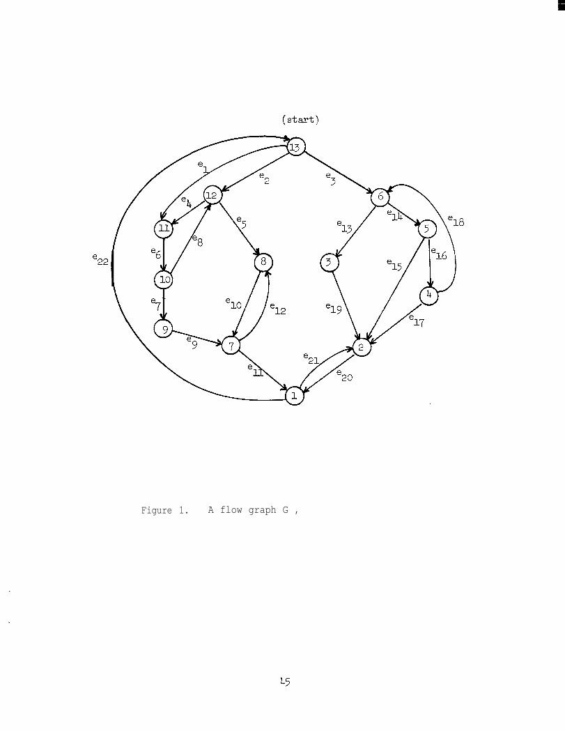
Lemma6 [l]. There is a tree T , called the dominator tree of G ,

such that v is a proper ancestor of w in T if and only if v

dominates w . Vertex r is the root of T and D contains every

vertex in G .

For any vertex v # r , we denote by idom(v) the parent of v

in T l Vertex idom(v) is called the immediate dominator of v and

is the unique vertex which daminates v and is dcminated by every othera

dominator of v . The dominator tree defines the single-entry regions

of G; the following lemma is a technical statement of this fact.

. (Note the similarity between this lemma and Lemma 3.)

Lemma7. For any edge e , idom(t(e)) is an ancestor of h(e) in T .

Proof, Every path fram r to t(e) contains idom(t(e)) . By adding

edge e to any path from r to h(e) , we get a path from r to t(e) .

33

Thus any path from r to h(e) contains idom(t(e)) , and by Lemma 6

idom(t(e)) z h(e) in T . 0

For any edge e , let g be an edge such that t(e) = t(e) and

h(“e) = h(e) if h(e) = idom(t(e)) , h(e) = u where

idom(t(e)) -+ u 5 h(e) in T if t(e) # idom(h(e)) . Let

E = (V,k,r) , where E = {e \ e E E} . We call g the derived graph

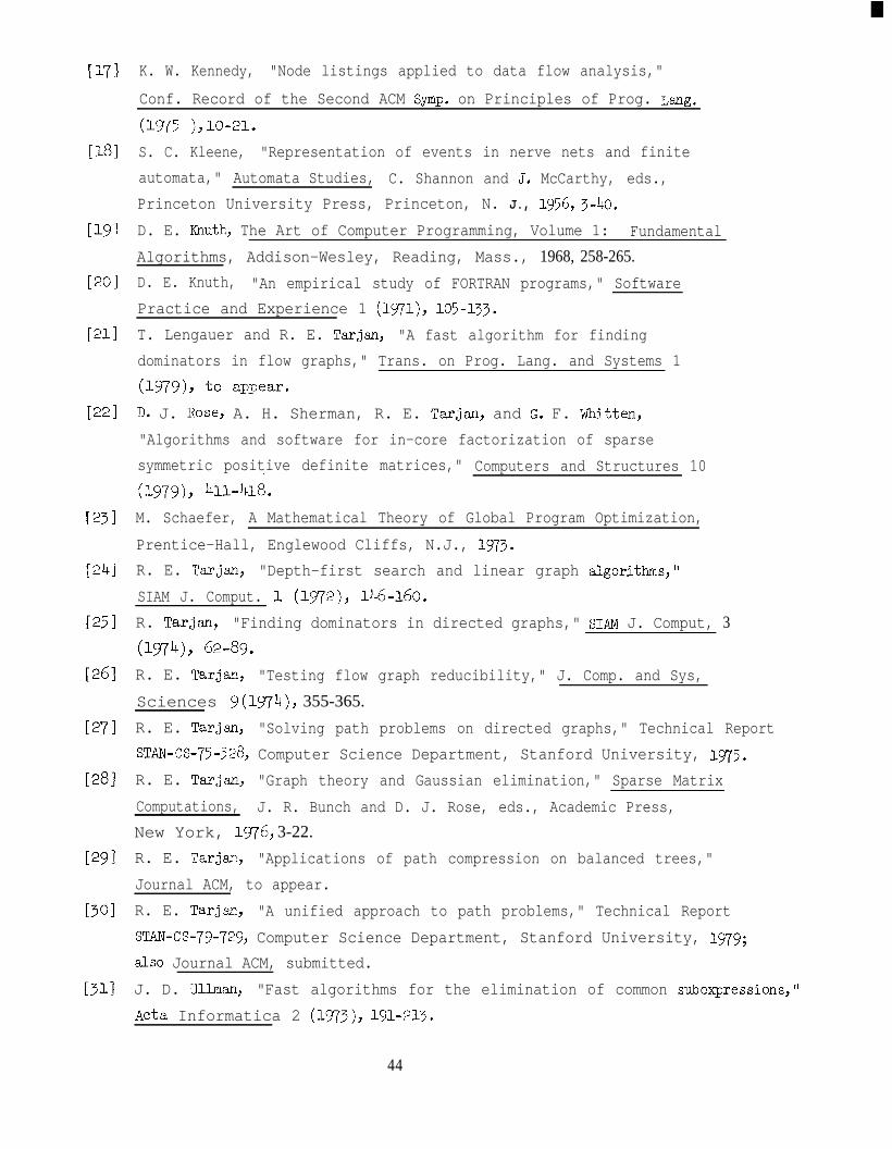
of G. Figures l-3 illustrate a graph, its dominator tree, and its

derived graph. Note that there are three kinds of edges in the derived

graph. If t(e) = idom(h(e)) , then g = e is an edge in T , If

t(e) 5 h(e) in T then < is a loop. Otherwise g leads from one

sibling to another in T .

[Figure l]

[Figure 21

[Figure 31

We call the strong ccmponents of ?! the daminator strong components

of G. It is not hard to prove that a graph is reducible if and only if

all its dominator strong components are single vertices. The idea of

our algorithm is to use Gaussian elimination (or saMe other method) toa

ccmpute a path sequence for each dominator strong component of 2 , and

to combine these path sequences to form a path

a ctibination of the methods in Sections 3 and

manipulates the dominator tree in the same way

sequence for G by using

5. The algorithm

that REDUCE AND SEQUENCE- -

manipulates the tree defined by the header pointers. Henceforth when

we refer to descendants and ancestors we mean with respect to the

dominator tree T .

34

The

that the

for each

for each

algorithm assumes that the dominator tree of G is known and

vertices are numbered from 1 to n so that idom(v) > v

vertex vf r . The algorithm requires the following information:

vertex u the set children(u) of vertices v such that

idom(v) = u , the set tree(u) of edges e such that t(e) = u and

h(e) = idom(u) , and the set nontree of edges e such that

t(e) = u and h(e) # idom(u) ; for each edge e the corresponding

edge e in L This information and the vertex numbering can be

computed in O(m a(m,n)) time using the dominators algorithm of

Lengauer and Tarjan [21].

The algorithm groups together vertices with a common parent and

processes these sibling sets in increasing order by parent. The algorithm

processes the set of siblings children(u) for each vertex u as

follows. For each edge e such that h(e) is a child of u , the

algorithm uses EVALJND~SEQUENCE to compute a path expression p(e)

representing all paths in G frcm h(e) to t(g) which end with

edge e and contain only proper descendants of h(g) as intermediate

vertices. Then the algorithm computes a path sequence Xu for the

- subgraph "Gu of 5 induced by children(u) . Substituting P(g) for

for each edge g appearing in this path sequence produces a sequence

yuthat represents every path in G starting and ending at a child

of u and containing only proper descendants of u as intermediate

vertices.

The algorithm concatenates Yu onto the end of the path sequence,

By applying SOLVE to Yu, the algorithm computes for each child v

of u a path expression R(v) which represents all paths in G from

35

u to v containing only proper descendants of u as intermediate

vertices. The algorithm completes the processing of the sibling set

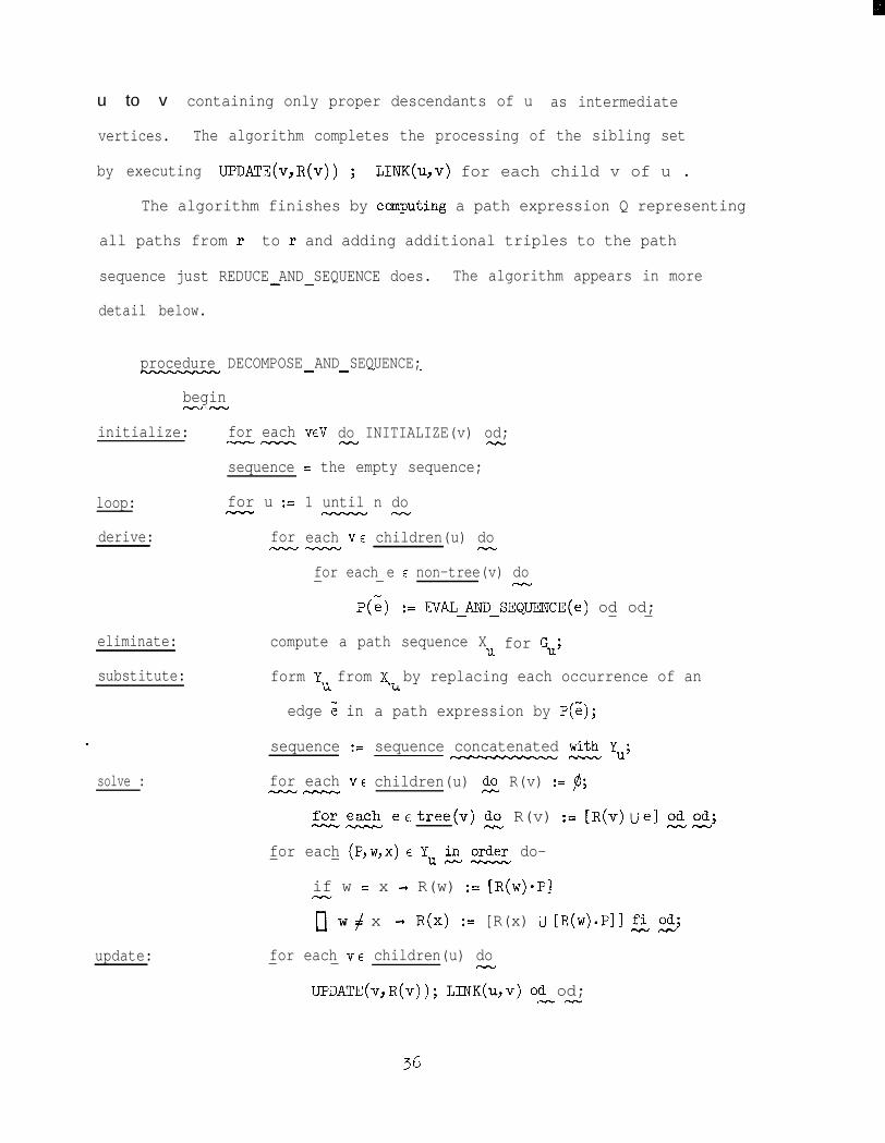
by executing UPDATE(v,R(v)) ; LINK(u,v) for each child v of u .

The algorithm finishes by camputing a path expression Q representing

all paths from r to r and adding additional triples to the path

sequence just REDUCE AND SEQUENCE does.- - The algorithm appears in more

detail below.

procedure DECOMPOSE AND SEQUENCE;

begin--NV

initialize: for eachTvw-

sequence

loop: for u :=-

derive: for each VE children(u) do-- -

eliminate:

substitute:

solve :

update:

WV do INITIALIZE(v) od;- -

= the empty sequence;

1 until n do-

for each e E non-tree(v) do- - -

p(e) := EVALJ.ND~SEQUENCE(e) od od;- -

compute a path sequence Xu for Gu;

form Y,, from X,, by replacing each occurrence of anU

edge g in

sequence :=

for each VENW-

U

a path expression by P(g);

sequence concatenated E Yu;

children(u) $o- R(v) := p;

ze eetree(v) 2 R(v) := [R(v)Ue] spd;

for each (P,w,x) E Yu g E do-- -

if w = x --) R(w) := [R(w)*P]

iiw x 3 R(x) := [R(x) U [R(w).P]] 2 g;

for each VE children(u) do- - -

UPDATE(v,R(v)); LINK(u,v) od od;r- -

36

finalize: Q p;:=

for each e enontree(r) do Q := [QUEVALJND-SEQUENCE(e)] od;- -

g [Q*] j! A add ([Q*],rF) to sequence 2;

-

for v-:= n-l b2 -1 El E add (S(v),, ancestor(v), v)

to sequence od-

end DECOMPOSE AND-SEQUENCE;-

This method combines the techniques of Section 3 with the method

of Section 5. The parts of the program labelled initialize , derive ,

update , and finalize are adapted from REDUCE AND SEQUENCE and serve- -

to combine the path sequences computed for the dominator strong components

( in eliminate-- and substitute ) into a path sequence for the entire

graph. The two loops labelled solve comprise a version of SOLVE,

We can implement step eliminate using ELIMINATE on the strong

components of iland combining the results as described in Theorem 6.

Step substitute can be performed either after or during the computation

of xU ; the latter is preferable.

The next lemma expresses the properties of the values computed by

DECOMPOSE AND ELIMINATE; its proof combines the ideas in Theorem 1 and- -- Corollary 1.

Lemma 8. (i) For each edge e in G such that eenontree(t(e)) ,

-P(e) as computed by DECOMPOSE AND SEQUENCE is a non-redundant path- -

expression representing exactly the paths in G from h(e) to t(e>

which end with edge e and contain only proper descendants of h(z)

as intermediate vertices.

(ii) For each vertex v in G , R(v) as computed by DECOMPOSEJND-SEQUENCE

is a non-redundant path expression representing exactly the paths in G

37

from idom(v) to v which contain only proper descendants of idom(v)

as intermediate vertices.

(iii) For each vertex u in G , Yu as computed by DECOMPOSEJND-SEQUENCE

is a sequence Yu = (pl~vl'wl~~ (Ppp& . . .j (Pp'vpd) satisfying

(64, (6b), ad.

(9) For any non-empty path p in G which starts and ends at a child

of u and contains only proper descendants of u as intermediate vertices,

there is a unique sequence of indices 1 <_ il < i2 < . . . < ik < 1 and-

a unique partition of p into non-empty paths p = pl,p2> l . .) 'k such

that pj E a(Pi ) for 1 < i < k .- -3

Proof. Straightforward by induction on the number of times the loop

in DECOMPOSE AND SEQUENCE is executed. I3- -

Theorem 9. Procedure DECOMPOSE AND SEQUENCE correctly computes a path- -

sequence for G .

Proof. Analogous to the proof of Theorem 8. 0

DECOMPOSE AND ELIMINATE thus provides a way to compute path sequences- -

- in arbitrary graphs. The running time of the method is O(m a(m,n)+t)

if stratified path compression is used to implement the forest operations

and O((m log n)+t) if path compression is used, where t is the time

to find path sequences for the dominator strong components of G . The

length of the path sequence produced is either O(m a(m,n))+ I or

O(m log n)+ I , where R is the total length of the path sequences for

the dominator strong components.

38

7. Remarks.

In this paper we have described fast algorithms for solving path

expression problems on reducible or almost-reducible graphs. The fastest

method requires O(m CX(m,n)+t) time to compute a path sequence for an

arbitrary directed graph, where t is the amount of time required to

compute path sequences for the dominator strong components. A slower

but much simpler method requires O(m log n + t) time and promises to

be easy to program and efficient in practice.

By using our algorithms in combination with the mapping technique

described by Tarjan [30], we can solve many kinds of path problems,

including finding shortest paths, carrying out forward and backward

global flow analysis, and solving sparse systems of linear equations.

There are two rather different ways of doing this. The first is to

use the solution to a path expression problem as a general-purpose

straight-line program which solves any particular path problem by

properly interpreting u , l , and * . The second is to use an algorithm

for solving a path expression problem to solve a particular path problem

by reinterpreting u , l , and * within the algorithm; this avoids the

- intermediate step of first constructing a directed acyclic graph

representing a set of path expressions. The choice between these two

methods depends upon the time and space available and whether we want

to solve one or many path problems on the same graph.

For path problems in which the operation corresponding to + is

idempotent, the non-redundancy and uniqueness conditions in (6) and

Theorem 1 are not necessary and can be dropped [30]. In such cases we

can use the sophisticated algorithm of Tarjan [29] to carry out the

39

forest manipulation operations and achieve an O(m a(m,n) +t) time

bound [27]. It does not seem possible to adapt this method to satisfy

non-redundancy, however. The only interesting path problem known to

the author which does not have the idempotent property is the solution

of sparse systems of linear equations. For this problem another form

of tree manipulation described by Tarjan [29] gives a rather simple

O(m a(m,n) +t) -time algorithm [28].

The method of decomposition by dominators is a kind of single-element

"tearing" [5] in which the clever use of data structures allows us to

make the combining step very efficient. The result may be generalizable

in various directions. For instance, on problem graphs for which there

is no natural start vertex we would like to know how to pick a start

vertex which gives the finest decomposition. It may also be possible

. to extend the technique to regions with two or more entry vertices. We

leave these questions to the ambitious reader.

40

Appendix: Graph Theoretic Terminology.

A directed graph G = (V,E) is a finite set V of vertices and a

finite set E of edges such that each edge e has a head h(e) EV and

a tail t(e) eV . We regard the edge e as leading from h(e) to t(e> 2

and we say the edge e leaves h(e) and enterst(e) l

We usually

denote the number of vertices by n and the number of edges by m .

A loop is an edge e with h(e) = t(e) . A path p = elJe2, . . .) ek is

a sequence of edges such that t(ei) = h(ei+l) for 1 < i < k-l . The- -

path is from h(p) = h(el) to t(p) = t(ek) . The path contains edges

el,e2,...,ek and vertices h(e1)‘h(e2L l l l 7 h(ek),t(ek) and avoids all

other edges and vertices. There is a path of no edges from any vertex

to itself. A cycle is a non-empty path from a vertex to itself. A graph

is acyclic if it contains no cycles.

The reverse Gr of a graph G is the graph formed by replacing

each edge e with an edge er such that h(er) = t(e) and t(er) = h(e) .

If Gl = @El) and G2 = (V2,E2) are graphs, Gl is a subgraph of

G2 if VlcV- 2 and ElcE .- 2

Gl is the subgraph of G2 induced by

vl if VlcV- 2 and El= p E E2 \ h(e),t(e) E V☺ l

-

A vertex v is reachable from a vertex w in a graph G if there

is a path from v to w. G is strongly connected if every vertex is

1 reachable from every other vertex. The strong components of G are its

maximal strongly connected subgraphs. These components are uniquely

defined and partition the vertices of G .

A flow graph G = (V,E,r) is a graph with a distinguished start

vertex r such that every vertex is reachable from r . A (directed,

rooted) tree T = (V,E,r) is a flow graph with \E\ = IV\-1 . The start

41

vertex r is the root of the tree. Any tree is acyclic, and if v

is any vertex in T , there is a unique path from r to v . If v

and w are vertices in a tree T and there is a path from v to w ,

V is an ancestor of w and w is a descendant of v . We denote*

this relationship by v 4w . If in addition Vfb v is a proper

+ancestor of w and w is a proper descendant of v , denoted by v -+w .

If there is an edge from v to w , v is the parent of w and w is

a child of v , denoted by v 3 w . Two vertices with a common parent

are siblings. In a tree each vertex has a unique parent (except the

root, which has no parent).

42

Cl1

PI

[31

v+l

[51

PI

171

PI

II91

PO1[=I

a [M

D31

D41

P51

b-61

References

A. V. Aho and J. D. Ullman, The Theory of Parsing, Translation, and

Compiling, Volume II: Compiling, Prentice-Hall, Englewood Cliffs,

N.J. (1972), 915.

A. V. Aho and J. D. Ullman, Principles of Compiler Design,

Addison-Wesley, Reading, Mass., 1977, 408-517.

F. E. Allen, "Control flow analysis," SIGPLAN Notices 5, 7 (19'70

l-19.

R. C. Backhouse and B. A. Car&, "Regular algebra applied to

> 7

path-finding problems," J. Inst. Maths. Applies. 15 (1975), 161-186.

J. R. Bunch and D. J. Rose, "Partitioning, tearing, and modification

of sparse linear systems," J. Math. Analysis and Applies. 48 (1974),

574-593 l

B. A. Car& "An algebra for network routing problems," J. Inst.

Math. Applies. 7 (lg'i'l), 273-294.

E. W. Dijkstra, A Discipline of Programming, Prentice-Hall,

Englewood Cliffs, N.J., 1976.

I. s. Duff, "A survey of sparse matrix research, r' Proc. IEEE 65 (1~77)~

500-535.R. Farrow, "Efficient variants of path compression on unbalanced

trees," unpublished manuscript, 1978.

R. Floyd, "Algorithm 97: shortest path," Comm. ACM 5 (1962), 345.

G. E. Forsythe and C. B. Moler, Computer Solution of Linear Algebraic

Equations, Prentice-Hall, Englewood Cliffs, N.J., 1967.

S. L. Graham and M. Wegman, "A fast and usually linear algorithm for

global flow analysis," Journal ACM 23 (1~76)~ 172-202.

M. S. Hecht, Flow Analysis of Computer Programs, Elsevier, New York,

1 9 7 7 l

M. S. Hecht and J. D. Ullman, "Flow graph reducibility," SIAM J.

Comput. 1 (lg72), 188-202.

M. S. Hecht and J. D. Ullman, "Characterizations of reducible flow

graphs," Journal ACM 21 (1974), 367-375.

D. B. Johnson, "Efficient algorithms for shortest paths in sparse

networks," Journal ACM 24 (1977), l-13.

43

Cl71

1181

P91

PO1

Pll

Pm

c231

v41

1251

WI

[271

P8l

1291

c301

[311

K. W. Kennedy, "Node listings applied to data flow analysis,"

Conf. Record of the Second ACM Symp. on Principles of Prog. Lang.

(1975 >, m-21.

S. C. Kleene, "Representation of events in nerve nets and finite

automata," Automata Studies, C. Shannon and J. McCarthy, eds.,

Princeton University Press, Princeton, N. J., 1956, 3-40.

D. E. Knuth, The Art of Computer Programming, Volume 1: Fundamental

Algorithms, Addison-Wesley, Reading, Mass., 1968, 258-265.

D. E. Knuth, "An empirical study of FORTRAN programs," Software

Practice and Experience 1 (lgl), 105-133.

T. Lengauer and R. E. Tarjan, "A fast algorithm for finding

dominators in flow graphs," Trans. on Prog. Lang. and Systems 1

(1979), to appear.

D. J. Rose, A. H. Sherman, R. E. Tarjan, and G. F. Whitten,

"Algorithms and software for in-core factorization of sparse

symmetric positive definite matrices,"

(1g7g), 411-418.

Computers and Structures 10

M. Schaefer, A Mathematical Theory of Global Program Optimization,

Prentice-Hall, Englewood Cliffs, N.J., 1973.

R. E. Tarjan, "Depth-first search and linear graph algorithms,rr

SIAM J. Comput. 1 (lg72), 146-160.

R. Tarjan, "Finding dominators in directed graphs," SIAM J. Comput, 3

(wi’4), 62-B.

R. E. Tarjan, "Testing flow graph reducibility," J. Comp. and Sys,

Sciences 9 (1~974)~ 355-365.

R. E. Tarjan, "Solving path problems on directed graphs," Technical Report

STAN-CS-75-528, Computer Science Department, Stanford University, 1975.

R. E. Tarjan, "Graph theory and Gaussian elimination," Sparse Matrix

Computations, J. R. Bunch and D. J. Rose, eds., Academic Press,

New York, 1976, 3-22.

R. E. Tarjan, "Applications of path compression on balanced trees,"

Journal ACM, to appear.

R. E. Tarjan, "A unified approach to path problems," Technical Report

STAN-CS-79-729, Computer Science Department, Stanford University, 1979;

also Journal ACM, submitted.

J. D. Ullman, "Fast algorithms for the elimination of common subexpressions,rr

Acta Informatica 2 (1973), 191-213.

44

(start)

Figure 1. A flow graph G ,

45

Figure 2. The dominator tree of G .

46

Figure 3. The derived graph of G . The vertex sets of the

dominator strong components are (uq 7 [33 7 (4) 7

{5] 7 161 7 C7783 7 (91 7 (lOI 7 p171q 7 Cl33 l

47