Fast and Informative Flow Simulations in a Building by Using Fast Fluid

Dynamics Model on Graphics Processing Unit

Wangda Zuo, Qingyan Chen

National Air Transportation Center of Excellence for Research in the Intermodal Transport Environment

(RITE), School of Mechanical Engineering, Purdue University, 585 Purdue Mall, West Lafayette, IN

47907-2088USA

Wangda Zuo

Email: wzuo@purdue.edu

Qingyan Chen (Corresponding Author)

Email: yanchen@purdue.edu

Phone: +1-765-496-7562

Fax: +1-765-494-0539

Abstract

Fast indoor airflow simulations are necessary for building emergency management, preliminary design

of sustainable buildings, and real-time indoor environment control. The simulation should also be

informative since the airflow motion, temperature distribution, and contaminant concentration are

important. Unfortunately, none of the current indoor airflow simulation techniques can satisfy both

requirements at the same time. Our previous study proposed a Fast Fluid Dynamics (FFD) model for

indoor flow simulation. The FFD is an intermediate method between the Computational Fluid Dynamics

(CFD) and multizone/zonal models. It can efficiently solve Navier-Stokes equations and other

transportation equations for energy and species at a speed of 50 times faster than the CFD. However,

this speed is still not fast enough to do real-time simulation for a whole building. This paper reports our

efforts on further accelerating FFD simulation by running it in parallel on a Graphics Processing Unit

(GPU). This study validated the FFD on the GPU by simulating the flow in a lid-driven cavity, channel

flow, forced convective flow, and natural convective flow. The results show that the FFD on the GPU can

produce reasonable results for those indoor flows. In addition, the FFD on the GPU is 10-30 times faster

than that on a Central Processing Unit (CPU). As a whole, the FFD on a GPU can be 500-1500 times

faster than the CFD on a CPU. By applying the FFD to the GPU, it is possible to do real-time informative

airflow simulation for a small building.

Key Words: Graphics Processing Unit (GPU), Airflow Simulation, Fast Fluid Dynamics (FFD), Parallel

Computing, Central Processing Unit (CPU)

Zuo, W. and Chen, Q. 2010. “Fast and informative flow simulations in a building by using fast fluid dynamics model on graphics processing unit," Building and Environment, 45(3), 747-757.

Nomenclature

ai,j, bi,j equation coefficient (dimensionless)

C contaminant concentration (kg/m3)

fi body force(kg /m2 s2)

H the width of the room (m)

i, j mesh node indices

kC contaminant diffusivity (m2/s)

kT thermal diffusivity (m2/s)

L length scale (m)

P pressure (kg/m·s2)

SC contaminant source (kg/m3s)

ST heat source (0C/s)

T temperature (0C)

t time (s)

ui,j velocity components at mesh node (i, j) (m/s)

Ub bulk velocity (m/s)

Ui, Uj velocity components in xi and xj directions, respectively (m/s)

U horizontal velocity or velocity scale (m/s)

V vertical velocity (m/s)

xi, xj spatial coordinates

x, y spatial coordinates

t time step (s)

kinematic viscosity (m2/s) 0 previous time step

1. Introduction According to the United States Fire Administration [1], 3,430 civilians and 118 firefighters lost their lives

in fires in 2007, with an additional 17,675 civilians injured. Smoke inhalation is responsible for most

fire-related injuries and deaths in buildings. Computer simulations can predict the transportation of

poisonous air/gas in buildings. If the prediction is in real-time or faster-than-real-time, firefighters can

follow appropriate rescue plans to minimize casualties. In addition, to design sustainable buildings that

can provide a comfortable and healthy indoor environment with less energy consumption, it is essential

to know the distributions of air velocity, air temperature, and contaminant concentration in buildings.

Flow simulations in buildings can provide this information [2]. Again, the predictions should be rapid due

to the limited time available during the design process. Furthermore, one can optimize the building

HVAC control systems if the indoor environment can be simulated in real-time or faster-than-real-time.

However, none of the current flow simulation techniques for buildings can satisfy the requirements for

obtaining results quickly and informatively. For example, CFD is an important tool to use in studying flow

and contaminant transport in buildings [3]. But when the simulated flow domain is large or the flow is

complex, the CFD simulation requires a large amount of computing meshes. Consequently, it needs a

very long computing time if it is only using a single processor computer [4].

A typical approach to reduce the computing time for indoor airflow simulations is to reduce the order of

flow simulation models. Zonal models [5] divide a room into several zones and assume that air property

in a zone is uniform. Based on this assumption, zone models only compute a few nodes for a room to

greatly reduce related computing demands. Multizone models [6] further expand the uniform

assumption to the whole room so that the number of computing nodes can be further reduced. These

approaches are widely used for air simulations in a whole building. However, the zonal and multizone

models solve only the mass continuity, energy, and species concentration equations but not the

momentum equations. They are fast but not accurate enough since they can only provide the bulk

information of each zone without the details about the airflow and contaminant transport inside the zone

[6].

Recently, a FFD method [7] has been proposed for fast flow simulations in buildings as an intermediate

method between the CFD and zonal/multizone models. The FFD method solves the continuity equation

and unsteady Navier-Stokes equations as the CFD does. By using a different numerical scheme to

solve the governing equations, the FFD can run about 50 times faster than the CFD with the same

numerical setting on a single CPU [8]. Although the FFD is not as accurate as the CFD, it can provide

more detailed information than a multizone model or a zonal model.

Although the FFD is much faster than the CFD, its speed is still not fast enough for the real-time flow

simulation in a building. For example, our previous work [8] found that the FFD simulation can be

real-time with 65,000 grids. If a simulation domain with 30 X 30 X 30 grids is applied for a room, the FFD

code can only simulate the airflow in 2-3 rooms on real-time. Hence, if we want to do real-time

simulation for a large building, we have to further accelerate the FFD simulation.

To reduce the computing time, many researchers have performed the flow simulations in parallel on

multi-processor computers [9, 10]. It is also possible to speed up the FFD simulation by running it in

parallel on multi-processor computers. However, this approach needs large investments in equipment

purchase and installation and a designated space for installing the computers and the related capacity

of the cooling system used in the space. In addition, the fees for the operation and maintenance of a

multi-processor computer are also nearly the same as those of several single processor computers of

the same capacity. Hence, multi-processor computers are a luxury for building designers or emergency

management teams.

Recently, the GPU has attracted attention for parallel computing. Different from a CPU, the GPU is the

core of a computer graphics card and integrates multiple processors on a single chip. Its structure is

highly parallelized to achieve high performance for displaying and processing graphics. For example, a

NVIDA GeForce 8800 GTX GPU, available since 2006, integrates 128 processors so that its peak

computing speed is 367 GFLOPS (Giga FLoating point Operation Per Second). Comparatively, the

peak performance of an INETL Core2 Duo 3.0 GHz CPU available at the same time is only about 32

GFLOPS [11]. Figure 1 compares the computing speeds of CPU and GPU. The speed gap between the

CPU and the GPU has been increasing since 2003. Furthermore, this trend is likely to continue in the

future. Besides GPU’s high performance, the cost of a GPU is low. For example, a graphics card with

NVIDIA GeForce 8800 GTX GPU costs only around $500. It can easily be installed onto a personal

computer and there are no other additional costs.

Thus, it seems possible to realize fast and informative indoor airflow simulations by using the FFD on a

GPU. This paper reports our efforts to implement the FFD model in parallel on a NVIDIA GeForce 8800

GTX GPU. The GPU code was then validated by simulating several flows that consist of the basic

features of indoor airflows.

2. Fast Fluid Dynamics Our investigation used the FFD scheme proposed by Stam [7]. The FFD applies a splitting method to

solve the continuity equation (1) and Navier-Stokes equations (2) for an unsteady incompressible flow:

¶=

¶0i

i

U

x, (1)

2

2

1i i i ij

j ij

U U U fPU

t x xx

, (2)

where Ui and Uj are fluid velocity components in xi and xj directions, respectively; is kinematic

viscosity; is fluid density; P is pressure; t is time; and fi are body forces, such as buoyancy force and

other external forces. The FFD splits the Navier-Stokes equations (2) into three simple equations (3),

(4), and (5). Then it solves them one by one.

i ij

j

U UU

t x

, (3)

2

2i i i

j

U U f

t x

, (4)

1i

i

U P

t x

, (5)

Equation (3) can be reformatted as

0i i ij

j

U U DUU

t x Dt

, (6)

where DUi/Dt is material derivative. This means that if we follow a flow particle, the flow properties, such

as velocities Ui, on this particle, will not change with time. Therefore, one can get the value of Ui by

finding its value at the previous time step. The current study used a first order semi-Lagrangian

approach [12] to calculate the value of Ui.

Equation (4) is a typical unsteady diffusion equation. One can easily solve it by using an iterative

scheme such as Gauss-Seidel iteration or Jacobi iteration. This work has applied the Jacobi iteration

since it can solve the equation in parallel.

Finally, it ensures mass conservation by solving equations (1) and (5) together with a

pressure-correction projection method [13]. The idea of the projection method is that the pressure

should be adjusted so that the velocities satisfy the mass conservation. Assuming Ui0 is the velocity

obtained from equation (4), equation (5) can be expanded to

0 1i i

i

U UP

t x

, (7)

where t is time step size and Ui is the unknown velocity, which satisfy the continuity Equation (1):

¶=

¶0i

i

U

x. (8)

Substituting equation (7) into (8), one can get

0 2

2i

i i

U t P

x x

. (9)

Solving equation (9), one can obtain P. Substituting P into equation (7), Ui will be known.

The energy equation can be written as:

2

2j T Tj j

T T TU k S

t x x

, (10)

where T is temperature, kT is thermal diffusivity, and ST is heat source. The FFD solves the equation (10)

in a similar way as equations (2) except for the pressure-correction projection for mass conservation.

Very similarly, the FFD also determines concentrations of species by the following transportation

equation:

2

2j C Cj j

C C CU k S

t x x

, (11)

where C is the species concentration, kC is the diffusivity, and SC is the source.

The FFD scheme was originally proposed for computer visualization and computer games [7, 14, 15]. In

our previous work [8, 16], the authors have studied the performance of the FFD scheme for indoor

environment by computing different indoor airflows. The results showed that the FFD is about 50 times

faster than the CFD. The FFD could correctly predict the laminar flow, such as a laminar flow in a

lid-driven cavity at Re=100 [16]. But the FFD has some problems in computing turbulent flows due to the

lack of turbulence treatments [8]. Although the FFD can capture the major pattern of the flow, it can not

compute the flow profile as accurate as the CFD does. We also tried to improve the FFD by adding

some simple turbulence treatments, but no general improvement was found yet. In addition, although

the FFD is much faster than the CFD, it can only do real-time simulation for a couple of rooms. In order

to apply the FFD for real-time simulation in a whole building, its computing speed has to be further

accelerated.

Obviously, more investigations can be done to improve the accuracy of the FFD scheme and enhance

the speed of the FFD simulation. The focus of this paper is the latter. The following parts reports our

efforts on reducing the computing time by implementing the FFD model in parallel on the GPU.

3. Graphics Processing Unit In order to reduce the computing time, this investigation performed the FFD simulation in parallel on a

GPU. Our program was written by using a Computer Unified Data Architecture (CUDA) programming

environment [11]. CUDA provides a C-like programming environment for the GPU. It divides a GPU into

three levels (Figure 2). The highest level is called “grid.” Each grid consists of multiple “blocks” and

every block has many “threads.” A thread is the basic computing unit of the GPU. Mathematical and

logic operations are performed on the threads.

This study used a NVIDIA GeForce GTX 8800 GPU. The GPU has 16 streaming multiprocessors (SMs)

[17], and each SM can hold up to 8 blocks or 768 threads at one time. Thus, the entire GPU can

simultaneously hold up to 12,288 threads. Because CUDA does not allow one block to spread into two

SMs, the allocation of the blocks is crucial to employ the full capacity of a GPU. For example, if a block

has 512 threads, then only one block can be assigned to one SM and the rest of the 256 threads in that

SM are unused. If a block contains 256 threads, then 3 blocks can share all the 768 threads of an SM so

that the SM can be fully used. Theoretically, the 8800 GTX GPU can reach its peak performance when

all 12,288 threads are running at the same time. Practically, the peak performance also depends on

many other factors, such as the time for reading or writing data with the memory.

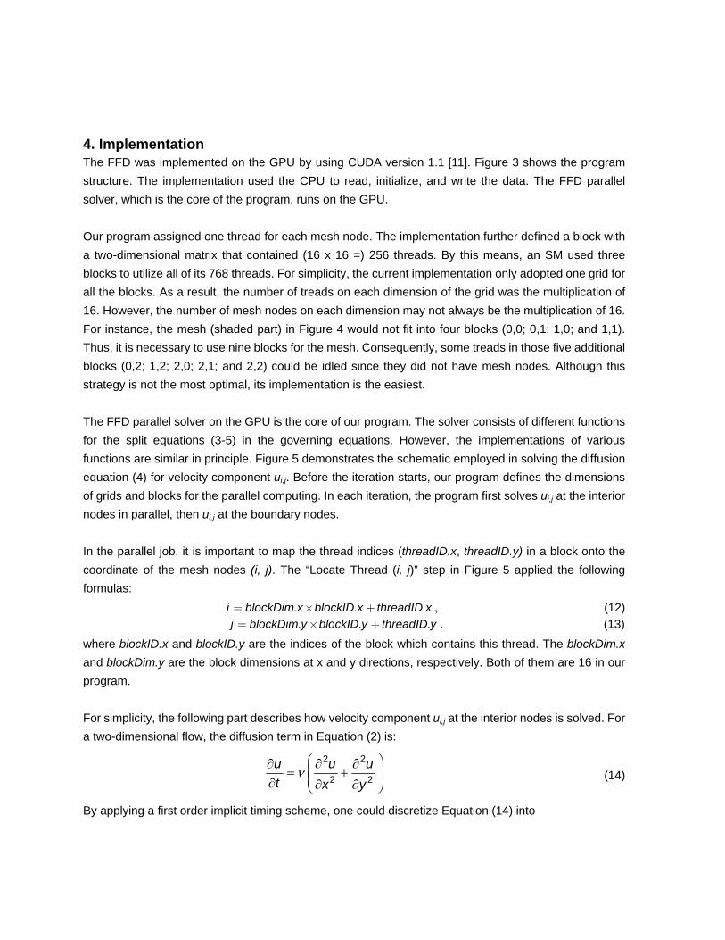
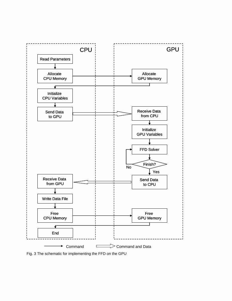
4. Implementation The FFD was implemented on the GPU by using CUDA version 1.1 [11]. Figure 3 shows the program

structure. The implementation used the CPU to read, initialize, and write the data. The FFD parallel

solver, which is the core of the program, runs on the GPU.

Our program assigned one thread for each mesh node. The implementation further defined a block with

a two-dimensional matrix that contained (16 x 16 =) 256 threads. By this means, an SM used three

blocks to utilize all of its 768 threads. For simplicity, the current implementation only adopted one grid for

all the blocks. As a result, the number of treads on each dimension of the grid was the multiplication of

16. However, the number of mesh nodes on each dimension may not always be the multiplication of 16.

For instance, the mesh (shaded part) in Figure 4 would not fit into four blocks (0,0; 0,1; 1,0; and 1,1).

Thus, it is necessary to use nine blocks for the mesh. Consequently, some treads in those five additional

blocks (0,2; 1,2; 2,0; 2,1; and 2,2) could be idled since they did not have mesh nodes. Although this

strategy is not the most optimal, its implementation is the easiest.

The FFD parallel solver on the GPU is the core of our program. The solver consists of different functions

for the split equations (3-5) in the governing equations. However, the implementations of various

functions are similar in principle. Figure 5 demonstrates the schematic employed in solving the diffusion

equation (4) for velocity component ui,j. Before the iteration starts, our program defines the dimensions

of grids and blocks for the parallel computing. In each iteration, the program first solves ui,j at the interior

nodes in parallel, then ui,j at the boundary nodes.

In the parallel job, it is important to map the thread indices (threadID.x, threadID.y) in a block onto the

coordinate of the mesh nodes (i, j). The “Locate Thread (i, j)” step in Figure 5 applied the following

formulas:

. . .i blockDim x blockID x threadID x= ´ + , (12) . . .j blockDim y blockID y threadID y= ´ + . (13)

where blockID.x and blockID.y are the indices of the block which contains this thread. The blockDim.x

and blockDim.y are the block dimensions at x and y directions, respectively. Both of them are 16 in our

program.

For simplicity, the following part describes how velocity component ui,j at the interior nodes is solved. For

a two-dimensional flow, the diffusion term in Equation (2) is:

2 2

2 2

u u u

t x y

(14)

By applying a first order implicit timing scheme, one could discretize Equation (14) into

1 2 1 2 1

2 2

t t t tu u u u

t x yn

+ + +æ ö- ¶ ¶ ÷ç ÷ç= + ÷ç ÷ç ÷D ç ¶ ¶è ø, (15)

where t is the time step, and the superscripts t and t+1 represent previous and current time steps,

respectively. Figure 6 illustrates the coordinates of the mesh. At mesh node (i, j), one can discretize

equation (15) in the space as:

, , 1, , , , ,t+1 t+1 t+1 t+1 t+1

i j i j i j i -1 j i+1 j i+1 j i, j -1 i, j -1 i, j+1 i, j+1 i ja u a u a u a u a u b-+ + + + = , (16)

where ai,j, ai-1,j, ai+1,j, ai,j-1 and ai,+1j are known coefficients. The bi,j on the right hand side of Equation (16),

which contains ui,jt , is also known. By this means, one can get a system of equations for all the interior

nodes. The equations can be solved in parallel by using the Jacobi iteration.

In general, our implementation of the FFD parallel solver on the GPU used the same principles as other

parallel computing on a multi-processor supercomputer. For more information on parallel computing,

one can refer to books [18-20].

5. Results and Discussion To evaluate the FFD on the GPU for indoor airflow simulation, this study compared the results of the

FFD on the GPU with the reference data. In addition, it was interesting to see the speed of the

simulations.

5.1. Evaluation of the Results

The evaluation was performed by using the FFD on the GPU to calculate four airflows relevant to the

indoor environment. The four flows were the flow in a lid-driven cavity, the fully developed flow in a plane

channel, the forced convective flow in an empty room, and the natural convective flow in a tall cavity.

The simulation results are compared with the data from the literature.

Flow in a Square Cavity Driven by a Lid

Air recirculated in a room is like the flow in a lid-driven cavity (Figure 7). This flow is also a classical case

for numerical validation [21]. This investigation studied both laminar and turbulent flows. Based on the

lid velocity of U = 1 m/s, cavity length of L = 1m, and kinematic viscosity of the fluid, the Reynolds

number of the laminar flow was 100 and the turbulent one was 10,000. A mesh with 65 x 65 grid points

was enough for a laminar flow with Re = 100. Since the FFD model had no turbulence model, it required

a dense mesh for the highly turbulent flow if an accurate result was desired. Thus, this study applied a

fine mesh with 513 x 513 grid points for the flow at Re = 10,000. The reference data was the high quality

CFD results obtained by Ghia et al [21].

Figure 8 compares the computed velocity profiles of the laminar flow (Re = 100) at the vertical (Figure

8a) and horizontal (Figure 8b) mid-sections with the reference data. The predictions by FFD on GPU are

the same as those for Ghia’s data for laminar flow. These results show that the FFD model works well

for laminar flow.

The flow at Re = 10,000 is highly turbulent. Although the current FFD model has no turbulence

treatment, it could still provide very accurate results by using dense mesh (513 x513). As shown in

Figure 9, the FFD on the GPU was able to accurately calculate the velocities at both vertical and

horizontal mid-sections of the cavity. The predicted velocity profiles agree with the reference data.

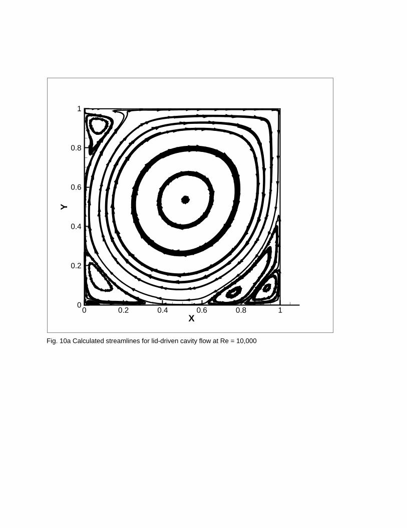
Figure 10 compares the streamlines calculated by the FFD with references ones [21]. The predicted

profiles (Figure 10a) of the vortices are similar to those of the reference one (Figure 10b). The FFD on

the GPU successfully computed not only the primary recirculation in the center of the cavity, but also the

secondary vortices in the upper-left, lower-left, and lower-right corners. There were one anti-clockwise

rotation in the upper-left corner, one anti-clockwise, and one other smaller clockwise rotation in both the

lower-left and lower-right corners. Although this is a simple case, it proves that the GPU could be used

for numerical computing as the CPU.

Flow in a Fully Developed Plane Channel

The flow in a long corridor can be simplified as a fully developed flow in a plane channel (Figure 11). The

Reynolds number of the flow studied was 2800, based on the mean bulk velocity Ub and the half

channel height, H. A mesh with 65 x 33 grid points was adopted by the FFD simulations. The Direct

Numerical Simulation (DNS) data from Mansour et al. [22] was selected as a reference. Figure 12

compares the predicted velocity profiles by the FFD on both the CPU and the GPU with the DNS data.

Different from the turbulent profile drawn by the DNS data, the FFD on the GPU, gave more laminar like

profiles. As discussed by the authors [8], this laminar profile was caused by a lack of turbulence

treatment in the current FFD model. Nevertheless, the GPU worked properly and the FFD on the GPU

was the same as that on the CPU for this case.

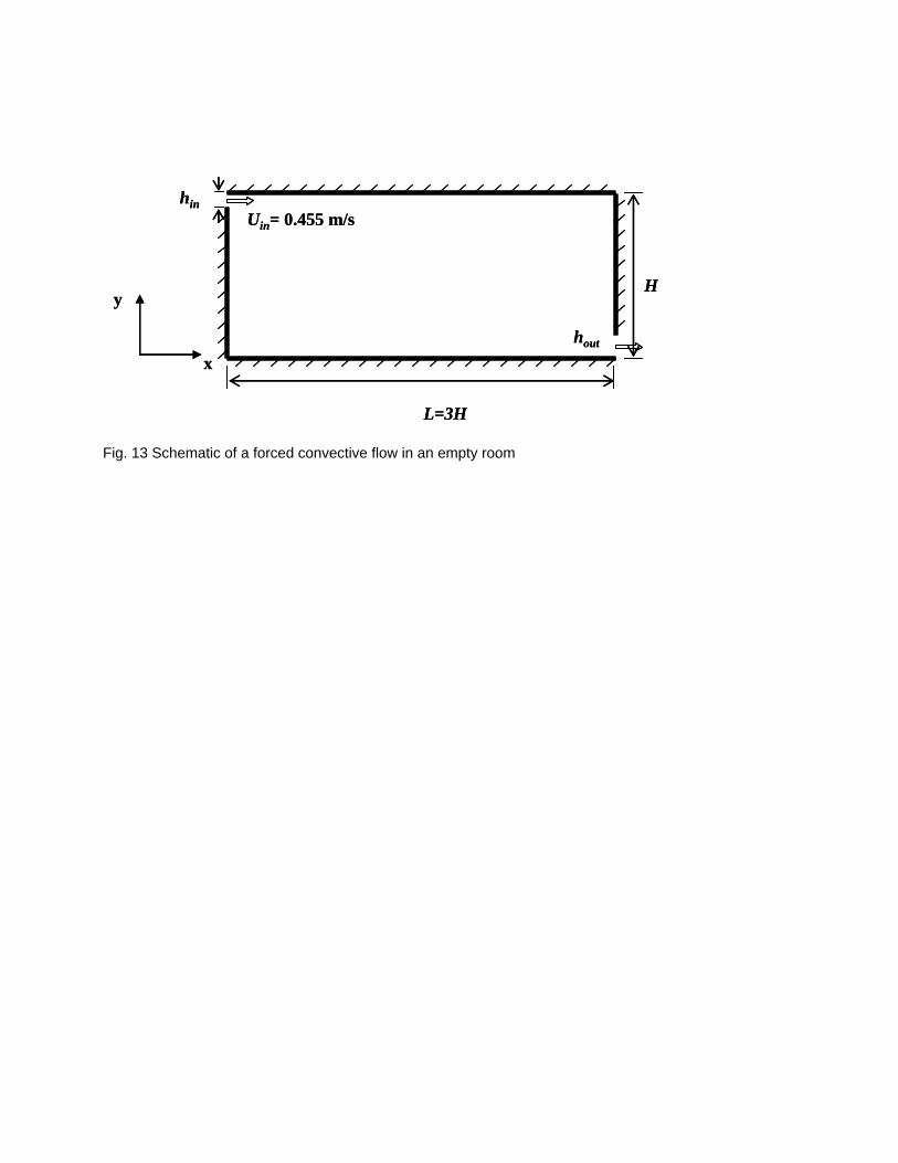
Flow in an Empty Room with Forced Convection

A forced convection flow in an empty room represents flows in mechanically ventilated rooms (Figure

13). The study was based on the experiment by Nielson [23]. His experimental data showed that the

flow in the room can be simplified into two-dimensions. The height of tested room, H, is 3m and the

width is 3H. The inlet was in the upper-left corner with a height of 0.56H. The outlet height was 0.16H

and located in the lower-right corner. The Reynolds number was 5000, based on the inlet height and

inlet velocity, which can lead to turbulent flow in a room. This study employed a mesh of 37 x 37 grid

points.

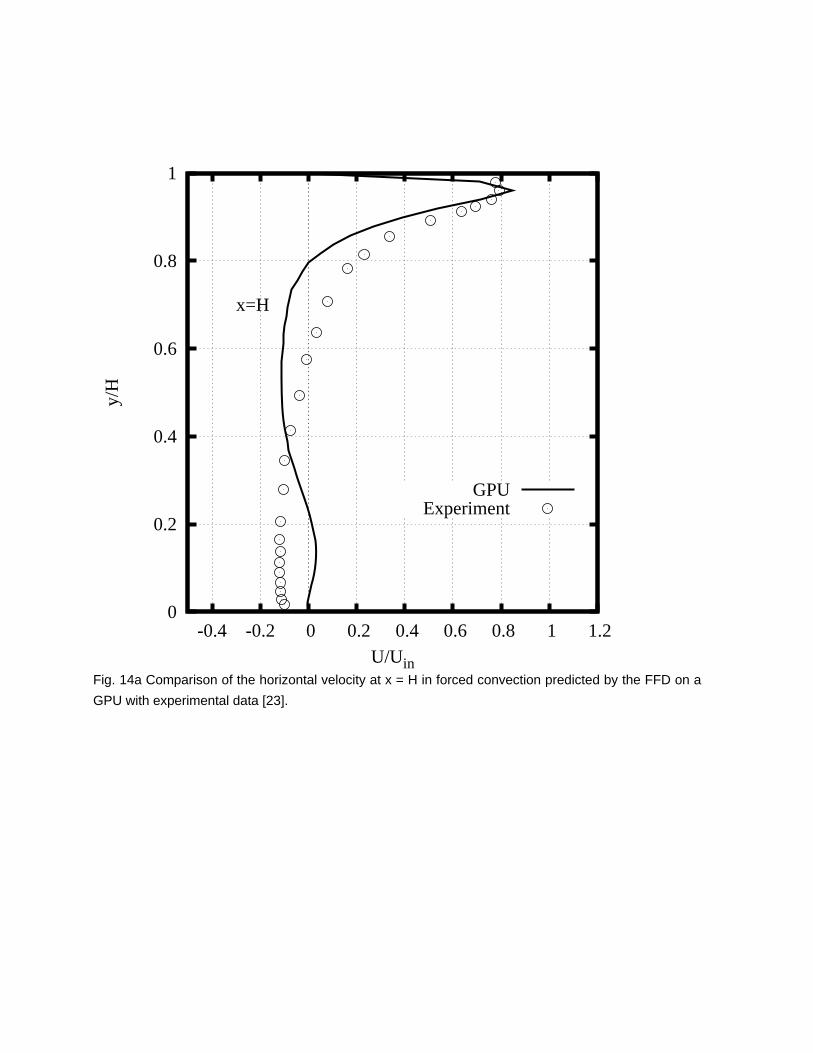
Figure 14 compares the predicted horizontal velocity profiles at the centers of the room (x = H and 2H)

and at the near wall regions (y = 0.028H and 0.972H) with the experimental data. As expected, the FFD

on the GPU could capture major characteristics of flow velocities (Fig. 14a and 14b). But the differences

between the prediction and experimental data are large at the near wall region (Figures 14c and 14d)

since we only applied a simple non-slip wall boundary condition. Advanced wall functions may improve

the results, but it will make the code more complex and require more computing time.

Flow in a Natural Convective Tall Cavity

The flows in the previous three cases were isothermal. The FFD on the GPU was further validated by

using a non-isothermal flow, such as a natural convection flow inside a dual window. This case was

based on the experiment by Betts and Bokhari [24]. They measured the natural convection flow in a tall

cavity of 0.076m wide and 2.18m high (Figure 15). The cavity was deep enough so that the flow pattern

was two-dimensional. The left wall was cooled at 15.1oC and the right wall heated at 34.7oC. The top

and bottom walls were isolated. The corresponding Rayleigh number was 0.86 x 106. A coarse mesh of

11 x 21 was applied. Figure 16 compares the predicted velocity and temperature with the experimental

data at three different lines across the cavity. The results show that the FFD on the GPU gave

reasonable velocity and temperature profiles. Again, the results obtained by the FFD on the GPU differ

from the experimental data, but they are the same as those of the FFD on the CPU. The results lead to a

similar conclusion as in the previous cases.

The above four cases show that the FFD code on the GPU produced accurate results for lid-driven

cavity flow and reasonable results for other airflows. Due to the limitation of the FFD model, predictions

by the FFD on the GPU may differ from the reference data.

5.2. Comparison of the Simulation Speed

To compare the FFD simulation speed on the GPU with that on the CPU, this study measured their

computing time for the lid-driven cavity flow. In addition, this study also measured the computing time by

the CFD on a CPU. A commercial CFD software FLUENT was used in the measurement. The

simulations were carried out on an HP workstation with an Intel XeonTM CPU and an NVIDIA GTX 8800

GPU. The data was for 100 time steps but with a different number of meshes.

Figure 17 illustrates that for both CFD and FFD, the CPU computing time increased linearly with the

mesh size. The CFD on the CPU was slower than on the FFD. There was a 50 times difference between

the CFD on the CPU and the FFD on the CPU. When the number of meshes was smaller than 3.6x103,

the FFD CPU version was faster than the GPU version. Since it took time to transfer data between the

CPU and the GPU during the GPU simulation, this part of the time could be more significant than that

saved in the parallel computing when the mesh size was small. Hence, the parallel computing on the

GPU should be applied to cases with a large mesh size.

One can also notice that the GPU computing time was almost constant when the mesh size was less

than 4x104. This is because the mesh size was not large enough so that the GPU could not fully use its

capacity. When the mesh size was greater than 4x104, the GPU computing time increased along two

paths. Those points on the solid line were for the cases with a mesh size in multiplication of 256 and on

the dashed line the mesh size could not be divided exactly by 256. As mentioned previously, each mesh

node was assigned to one thread and a block had 256 threads. If the mesh size was exactly the

multiplication of 256, all the 256 threads in every block were used. Thus, the working loads among

blocks were equal. Otherwise, some of the threads in the block were idled and the working loads

between the blocks were unequal. An imbalance in GPU working loads can impose a severe penalty on

the computing speed. For example, the case with 640 x 640 meshes that was a multiplication of 256

took 9.977 s, but that with 639 x 639 took 28.875 s. Although the latter case had fewer meshes than the

former, it took almost three times as much computing time.

Nevertheless, the FFD on the GPU is still much faster than on the CPU even if the cases were on the

dash line. The computing time of the GPU points on the dashed line was about 10 times shorter than

that of the CPU. The difference increased to around 30 times when the right amount of meshes was

used (solid line). Considering that the FFD on the CPU is 50 times faster than the CFD on the CPU, the

FFD on the GPU can be 500 –1500 times faster than the CFD on the CPU.

5.3. Discussion

This study implemented the FFD solver for flow simulation on the GPU. Since the FFD solves the same

governing equations as the CFD, it is also possible to implement the CFD solver on the GPU by using a

similar strategy. One can also expect that the speed of CFD simulations on the GPU should be faster

than that on the CPU. For the CFD codes written in C language, the implementation will be relatively

easy since only the parallel computing part needs to be rewritten in CUDA.

Current GPU computing speed can be further accelerated by optimizing the code implementation. The

dimensions of GPU blocks can be flexible to adapt to the mesh. Meanwhile, many classical optimization

techniques for paralleling computing are also good for GPU computing. For example, to read or write

data from GPU memory is time consuming, so the processors are often idled for data transmission. One

approach is to reuse the data already on the GPU by calculating several neighboring mesh nodes with

one thread.

In addition, the computing time can be further reduced by using multiple GPUs. For example, a NVIDIA

Tesla 4-GPU computer has 960 processors and 16 GB system memory [25]. Its peak performance can

be as high as 4 Tetra FLOPS, which is about 10 times faster than the GPU used in this study. Thus, the

computing time of a problem with large meshes can be greatly reduced by using multiple GPUs.

6. Conclusions This paper introduced an approach to conducting fast and informative indoor airflow simulation by using

the FFD on the GPU. An FFD code has been implemented in parallel on a GPU for indoor airflow

simulation. By applying the code for flow in a lid driven cavity, a channel flow, a forced convective flow,

and a natural convective flow, this investigation showed that the FFD on a GPU could predict indoor

airflow motion and air temperature. The prediction was the same as the data in the literature for

lid-driven cavity flow. The FFD on GPU can also capture major flow characteristics for other cases,

including fully developed channel flow, forced convective flow and natural convective flow. But some

differences exist due to the limitations of the FFD model, such as lack of turbulence model and simple

no-slip wall treatment.

In addition, a flow simulation with the FFD on the GPU was 30 times faster than that on the CPU when

the mesh size was the multiplication of 256. If the mesh size cannot be exactly the multiplication of 256,

the simulation was still 10 times faster than that on the CPU. As a whole, the FFD on a GPU can be 500

–1500 times faster than the CFD on a CPU.

7. Acknowledgements This study was funded by the US Federal Aviation Administration (FAA) Office of Aerospace Medicine

through the National Air Transportation Center of Excellence for Research in the Intermodal Transport

Environment under Cooperative Agreement 07-CRITE-PU and co-funded by the Computing Research

Institute at Purdue University. Although the FAA has sponsored this project, it neither endorses nor

rejects the findings of this research. The presentation of this information is in the interest of invoking

technical community comment on the results and conclusions of the research.

References 1. United States Fire Admin istration. Fire statisti cs. 200 8

http://www.usfa.dhs.gov/statistics/national/index.shtm. 2. Chen Q., C hapter 7: Design of natural v entilation with CFD, i n: L.R . Glick sman and J. Lin, Ed itors.

Sustainable urban housing in china. Springer; 2006, p. 116-123. 3. Nielsen P.V., Computational fluid dynamics and room air movement. Indoor Air 2004; 14:134-143. 4. Lin C., Horstman R., Ahlers M., Sedgwick L., Dunn K., Wirogo S., Numerical simulation of airflow and

airborne pathogen transport in aircraft cabins - part 1: Numerical simulation of the flow field. ASHRAE Transactions 2005; 111.

5. Megri A.C., Haghighat F. , Z onal m odeling f or si mulating i ndoor en vironment o f buildings: R eview, recent developments, and applications. HVAC&R Research 2007; 13(6):887-905.

6. Chen Q., Ventilation performance prediction for buildings: A method overview and recent applications. Building and Environment 2009; 44(4):848-858.

7. Stam J. St able fl uids. P roceedings of 26th I nternational C onference o n C omputer G raphics a nd Interactive Techniques (SIGGRAPH’99). 1999; Los Angeles.

8. Zuo W., Chen Q., Real-time or faster-than-real-time simulation of airflow in buildings. Indoor Air 2009; 19(1):33-44.

9. Mazumdar S., Chen Q., Influence of cabi n c onditions on placem ent and res ponse of c ontaminant detection sensors in a commercial aircraft. Journal of Environmental Monitoring 2008; 10(1):71-81.

10. Hasama T., Kato S., Ooka R., Analysis of wind-induced inf low and outflow through a sing le opening

using LES & D ES. Jou rnal of W ind Engineering and I ndustrial A erodynamics 2008; 96(10-11):1678-1691.

11. NVIDIA, N VIDIA C UDA c ompute uni fied de vice arc hitecture-- p rogramming g uide (ve rsion 1 .1). Santa Clara, California: NVIDIA Corporation; 2007.

12. Courant R., Isaacson E., Rees M., On the solution of nonlinear hyperbolic differential equations by finite differences. Communication on Pure and Applied Mathematics 1952; 5:243–255.

13. Chorin A .J., A numerical m ethod f or s olving i ncompressible vi scous fl ow problems. Jo urnal of Computational Physics 1967; 2(1):12-26.

14. Harris M .J., Real-time cl oud simulation and rendering. Ph .D. Th esis, Un iversity o f North Caro lina at Chapel Hill. 2003.

15. Song O.-Y., Shin H. , Ko H. -S., Stable but nondissipative water. ACM Transactions on Graphics 2005; 24(1): 81-97.

16. Zuo W., Chen Q. Val idation of fast fluid dynamics for r oom airflow. Proceedings of the 1 0th International IBPSA Conference (Building Simulation 2007). 2007; Beijing, China.

17. Rixner S., Stream processor architecture. Boston & London: Kluwer Academic Publishers; 2002. 18. Roosta S.H., Parallel processing and parallel algorithms: Theory and computation. New York: Springer;

1999. 19. Bertsekas D.P., Tsitsiklis J.N., Parallel an d distributed co mputation: Nu merical meth ods. Belm ont,

Massachusetts: Athena Scientific; 1989. 20. Lewis T.G., El-Rewini H., Kim I.-K., Introduction to parallel computing. Englewood Cliffs, New Jersey:

Prentice Hall; 1992. 21. Ghia U ., G hia K .N., S hin C .T., High-Re s olutions f or i ncompressible flow usi ng t he Na vier-Stokes

equations and a multigrid method. Journal of Computational Physics 1982; 48(3):387-411. 22. Mansour N.N., Kim J., Moin P., Reynolds-stress and dissipation-rate budgets in a turbulent channel flow.

Journal of Fluid Mechanics 1988; 194:15-44. 23. Nielsen P. V., Specification of a t wo-dimensional t est case. Aal borg, Denmark: Aal borg U niversity;

1990. 24. Betts P.L., B okhari I.H., Ex periments o n tu rbulent n atural co nvection in an en closed tall cav ity.

International Journal of Heat and Fluid Flow 2000; 21(6):675-683. 25. N VIDIA. 2009 http://www.nvidia.com/object/tesla_computing_solutions.html.

Figure Captions

0

50

100

150

200

250

300

350

400

2003 2004 2005 2006 2007

GFL

OPS

year

GPUCPU

Fig. 1 Comparison of the computing speeds of GPU (NVIDIA) and CPU (INTEL) since 2003 [11]

Host (CPU)

Device (GPU)

Grid 1

Grid 2

Grid 3, 4, …….

Block (2,2)

Block (1,2)

Block (0,2)

Block (2,1)

Block (1,1)

Block (0,1)

Block (2,0)

Block (1,0)

Block (0,0)

Block (2,2)

Block (1,2)

Block (0,2)

Block (2,1)

Block (1,1)

Block (0,1)

Block (2,0)

Block (1,0)

Block (0,0)

Grid 1 Grid 2 G

Block (2,2)

Block (1,2)

Block (0,2)

Block (2,1)

Block (1,1)

Block (0,1)

Block (2,0)

Block (1,0)

Block (0,0)

Block (2,2)

Block (1,2)

Block (0,2)

Block (2,1)

Block (1,1)

Block (0,1)

Block (2,0)

Block (1,0)

Block (0,0)

Thread (2,2)

Thread (1,2)

Thread (0,2)

Thread(2,1)

Thread (1,1)

Thread (0,1)

Thread (2,0)

Thread (1,0)

Thread(0,0)

Thread (2,2)

Thread (1,2)

Thread (0,2)

Thread(2,1)

Thread (1,1)

Thread (0,1)

Thread (2,0)

Thread (1,0)

Thread(0,0)

Block(0,0)

…

Thread (2,2)

Thread (1,2)

Thread (0,2)

Thread(2,1)

Thread (1,1)

Thread (0,1)

Thread (2,0)

Thread (1,0)

Thread(0,0)

Thread (2,2)

Thread (1,2)

Thread (0,2)

Thread(2,1)

Thread (1,1)

Thread (0,1)

Thread (2,0)

Thread (1,0)

Thread(0,0)

Block(1,0)

…………

Fig. 2 The schematic of parallel computing on CUDA

Read Parameters

Allocate CPU Memory

Initialize CPU Variables

FFD Solver

Finish?

Allocate GPU Memory

Initialize GPU Variables

Write Data File

Free CPU Memory

Free GPU Memory

End

Send Data to GPU

Receive Data from CPU

Send Data to CPU

Receive Data from GPU

CPU GPU

YesNo

Read Parameters

Allocate CPU Memory

Initialize CPU Variables

FFD Solver

Finish?

Allocate GPU Memory

Initialize GPU Variables

Write Data File

Free CPU Memory

Free GPU Memory

End

Send Data to GPU

Receive Data from CPU

Send Data to CPU

Receive Data from GPU

CPU GPU

YesNo

Command Command and Data

Fig. 3 The schematic for implementing the FFD on the GPU

Block (2,2)

Block (1,2)

Block (0,2)

Block (2,1)

Block (1,1)

Block (0,1)

Block (2,0)

Block (1,0)

Block (0,0)

Block (2,2)

Block (1,2)

Block (0,2)

Block (2,1)

Block (1,1)

Block (0,1)

Block (2,0)

Block (1,0)

Block (0,0)

Fig. 4 Allocation of mesh nodes to GPU blocks.

Interior Node?

Define Grids and Blocks

Start Parallel Job for Interior Nodes

Start Parallel Jobfor Boundary Nodes

Parallel Job

Locate Thread (i, j)

Calculate ui,j(n+1)

Iteration?

Yes

No

Boundary Node?

Parallel Job

Locate Thread (i, j)

Yes

No

Calculate ui,j(n+1)

Exit

Yes

……

……

……

……

No

Fig. 5 Schematic of implementation for solving diffusion term for velocity component u

i, j i+1, j

i, j+1

i–1, j

i, j-1

i, j i+1, j

i, j+1

i–1, j

i, j-1

Fig. 6 Coordinates for the computing meshes

U=1m/s

U=V=0 U=V=0

U=V=0

Fig. 7 Schematic of the flow in a square lid-driven cavity

0

0.2

0.4

0.6

0.8

1

-0.4 -0.2 0 0.2 0.4 0.6 0.8 1 1.2

y(m

)

U(m/s)

GPUGHIA

Fig. 8a Comparison of the calculated horizontal velocity profile (Re = 100) at x = 0.5 m with Ghia’s data

[21].

-0.6

-0.4

-0.2

0

0.2

0.4

0.6

0 0.2 0.4 0.6 0.8 1

V(m

/s)

x(m)

GPUGHIA

Fig. 8b Comparison of the calculated vertical velocity profile (Re = 100) at y = 0.5 m with Ghia’s data

[21].

0

0.2

0.4

0.6

0.8

1

-0.6 -0.4 -0.2 0 0.2 0.4 0.6 0.8 1 1.2

y(m

)

U(m/s)

FFD on GPUGHIA

Fig. 9a Comparison of the calculated horizontal velocity profiles (Re = 10,000) at x = 0.5m with Ghia’s

data [21].

-0.6

-0.4

-0.2

0

0.2

0.4

0.6

0 0.2 0.4 0.6 0.8 1

V(m

/s)

x(m)

FFD on GPUGHIA

Fig. 9b Comparison of the calculated vertical velocity profile (Re = 10,000) at y = 0.5m with Ghia’s data

[21].

X

Y

0 0.2 0.4 0.6 0.8 10

0.2

0.4

0.6

0.8

1

Fig. 10a Calculated streamlines for lid-driven cavity flow at Re = 10,000

Fig. 10b Ghia’s data [21] for streamlines for lid-driven cavity flow at Re = 10,000

UinUin

Fig. 11 Schematic of the fully developed flow in a plane channel

0

0.2

0.4

0.6

0.8

1

1.2

0 0.2 0.4 0.6 0.8 1

U/U

b

y/H

GPUCPUDNS

Fig. 12 Comparison of the mean velocity profile in a fully developed channel flow predicted by the FFD

on a GPU with the DNS data [22]

hin

hout

L=3H

Hy

x

Uin= 0.455 m/shin

hout

L=3H

Hy

x

Uin= 0.455 m/s

Fig. 13 Schematic of a forced convective flow in an empty room

0

0.2

0.4

0.6

0.8

1

-0.4 -0.2 0 0.2 0.4 0.6 0.8 1 1.2

y/H

U/Uin

x=H

GPUExperiment

Fig. 14a Comparison of the horizontal velocity at x = H in forced convection predicted by the FFD on a

GPU with experimental data [23].

0

0.2

0.4

0.6

0.8

1

-0.4 -0.2 0 0.2 0.4 0.6 0.8 1 1.2

y/H

U/Uin

x=2H

GPUExperiment

Fig. 14b Comparison of the horizontal velocity at x = 2H in forced convection predicted by the FFD on a

GPU with experimental data [23].

-0.5

0

0.5

1

1.5

0 0.5 1 1.5 2 2.5 3

U/U

in

x/H

y=0.028H

GPUExperiment

Fig. 14c Comparison of the horizontal velocity at y = 0.028H in forced convection predicted by the FFD

on a GPU with experimental data [23].

-0.5

0

0.5

1

1.5

0 0.5 1 1.5 2 2.5 3

U/U

in

x/H

y=0.972H

GPUExperiment

Fig. 14d Comparison of the horizontal velocity at y = 0.972H in forced convection predicted by the FFD

on a GPU with experimental data [23].

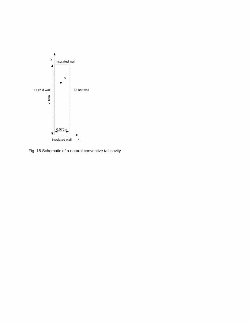
Fig. 15 Schematic of a natural convective tall cavity

0

0

0

0 0.02 0.04 0.06 0.076

0

0

0

V(m

/s)

V(m

/s)

x(m)

y=0.218m

y=1.090m

y=1.926m

GPUExperiment

Fig. 16a Comparison of the velocity profiles predicted by the FFD on a GPU with the experimental data

[24]

0 0.02 0.04 0.06 0.076

T(o C

)

T(o C

)

x(m)

y=0.218m

y=1.090m

y=1.926m

15.1

15.1

15.1

34.7

34.7

34.7

GPUExperiment

Fig. 16b Comparison of the temperature profiles predicted by the FFD on a GPU with the experimental

data [24]

1.0E-02

1.0E-01

1.0E+00

1.0E+01

1.0E+02

1.0E+03

1.0E+04

1.0E+05

1.0E+02 1.0E+03 1.0E+04 1.0E+05 1.0E+06 1.0E+07

Number of Grids

Com

putin

g T

ime

FFD on GPU

FFD on CPU

CFD on CPU

1.0E-02

1.0E-01

1.0E+00

1.0E+01

1.0E+02

1.0E+03

1.0E+04

1.0E+05

1.0E+02 1.0E+03 1.0E+04 1.0E+05 1.0E+06 1.0E+07

Number of Grids

Com

putin

g T

ime

FFD on GPU

FFD on CPU

CFD on CPU

Fig. 17 Comparison of the computing time used by the FFD on a GPU, the FFD on a CPU, and the CFD

on a CPU