Fast Anisotropic Smoothing of Multi-Valued Imagesusing Curvature-Preserving PDE’s

David Tschumperle

Equipe Image/GREYC (UMR CNRS 6072)6 Bd du Marechal Juin, 14050 Caen Cedex, France

Abstract

We are interested in PDE’s (Partial Differential Equations) in order to smooth multi-valued images in an anisotropicmanner. Starting from a review of existing anisotropic regularization schemes based on diffusion PDE’s, we point out thepros and cons of the different equations proposed in the literature. Then, we introduce a new tensor-driven PDE, regularizingimages while taking the curvatures of specific integral curves into account. We show that this constraint is particularly wellsuited for the preservation of thin structures in an image restoration process. A direct link is made between our proposedequation and a continuous formulation of the LIC’s (Line Integral Convolutions by Cabral and Leedom [11]). It leads tothe design of a very fast and stable algorithm that implements our regularization method, by successive integrations ofpixelvalues along curved integral lines. Besides, the scheme numerically performs with a sub-pixel accuracy and preserves thenthin image structures better than classical finite-differences discretizations. Finally, we illustrate the efficiency of our genericcurvature-preserving approach - in terms of speed and visual quality - with different comparisons and various applicationsrequiring image smoothing : color images denoising, inpainting and image resizing by nonlinear interpolation.

Keywords : Multi-valued Images, Data Regularization, Anisotropic Smoothing, Diffusion PDE’s, Tensor-valued Geometry,Denoising, Inpainting, Nonlinear Interpolation.

1 Introduction

Obtaining regularized versions of noisy or corrupted imagedata has always been a desirable goal in the fields of computervision and image processing. It is useful, either to restoredegraded images (which is the most direct application of imageregularization methods) or - more indirectly - as a pre-processing step that eases further analysis of the considered data.Regularization is actually one of the key operations neededby many image analysis algorithms. A lot of image regularizationformalisms have been then already proposed in the literature for this purpose.Since the pioneering work of Perona-Malik [33] in the early 90’s, the framework of anisotropic diffusion PDE’s (PartialDifferential Equations) has particularly raised a strong interest for data regularization : such equations have the ability tosmooth data in a nonlinear way, allowing the preservation ofsignificant image discontinuities. PDE’s are local formulationsand thus, they are well adapted to deal with degraded images where sources of data corruption are local or semi-local too :gaussian noise, scratches or compression artefacts are local degradations usually encountered in digital (original or digitized)images. Therefore, many variants of diffusion PDE’s have been proposed so far for the restoration of image datasets. Inparticular, important contributions in this field concern the way the classical isotropic diffusion equation (heat flow) hasbeen extended to deal with anisotropic smoothing [33, 27, 37, 52], how diffusion PDE’s may be seen as gradient descentsof various energy functionals [4, 13, 16, 23, 36], and the link between regularization PDE’s and the concept of non-linearscale spaces [1, 28, 30]. Extensions of these techniques to color images and more generally multi-valued datasets have beenalso tackled in [38, 44, 48, 53]. More recently, regularization PDE’s under constraints have been proposed in order to dealwith more specific datasets, as fields of unit vectors [18, 24,32, 41], orthonormal matrices [17, 45], positive-definite matrices[17, 46], or image data defined on implicit surfaces [7, 14, 42].Despite this wide range of existing constrained and unconstrained PDE formalisms, all regularization methods have some-thing in common : they locallysmooththe image along one or several directions of the plane that are different at each image

1

point. Typically, the principal smoothing directions are chosen to be parallel to the image contours, resulting in ananisotropicregularization that does not destroy edges. As a requirement, defining a correctsmoothing behavioris one of the first aim ofa good regularization algorithm, the second being the precision of the smoothing process itself : it must respect the definedsmoothing geometry as much as possible.Following this general principle, authors of [48, 52] recently proposed two different PDE-based frameworks able to designspecific regularization processes from a given (user-defined) underlying local smoothing geometry. These methods havetwomain interests : on one hand, they unify a lot of previously proposed equations into generic diffusion PDE’s and providea localgeometric interpretationof the corresponding regularizations. On the other hand, they clearly separate the designof the smoothing geometry from the smoothing process itself: in a first step, one retrieves the geometry of the structuresinside the image (generally by the computation of the so-called structure tensor fieldG). Then, a local geometry of thedesired smoothing is defined by the mean of a second fieldT of diffusion tensors(depending onG). Finally, one step ofthe smoothing process itself (driven byT) is performed through one or several iterations of a specificdiffusion PDE. Thisprocedure is repeated until the image is regularized enough.

In this article, we first review these two efficient and unifying regularization methods acting on unconstrained multi-valuedimages, following our interpretation of separating the smoothing from the geometry (section 2). We particularly pointoutthe advantages and drawbacks of each equation in real cases.We propose then a comparable tensor-driven diffusion PDEthat regularizes multi-valued images while respecting specific curvature constraints(section 3). Actually, our equation ismathematically positioned between the two previous formulations, in a way that it solves the issues inherent to both methods.Moreover, we propose a theoretical interpretation of our curvature-constrained formalism in terms of LIC’s (Line IntegralConvolutions [11]). This analogy leads to the proposal of a novel numerical scheme that implements our PDE (section 4),by successive integrations of pixel values along integral lines. This iterative scheme has two main advantages compared toclassical PDE implementations : on one hand, it preserves the orientations of thin image structures, since it naturallyworksat a sub-pixel accuracy. On the other hand, the algorithm is able to run up to three times faster than classical explicit schemesince it is unconditionally stable, even for large PDE time steps. Finally, we illustrate the effectiveness of our curvature-preserving method, in terms of computational speed and visual quality, with results on color image restoration, color imageinpainting and non-linear resizing, among all possible applications in the area of image regularization (section 5).

2 Anisotropic Smoothing of Images with PDE’s : A Review

Let us consider a multi-valued imageI : Ω → Rn (n = 3 for color images) corrupted by noise and defined on a domain

Ω ⊂ R2. We denote byIi : Ω → R, the scalar channeli of I : ∀X = (x, y) ∈ Ω, I(X) =

(

I1(X) I2(X) ... In(X)

)T.

RegularizingI can be done by one among the large variety of existing diffusion PDE’s. We will focus anyway on the recentworks in [48, 52], which are unifying approaches.

2.1 Local Geometry and Diffusion Tensors

Basically, PDE-based regularization may be seen as the local smoothing of an imageI along defined directions dependingthemselves on the local configuration of the pixel intensities. One wants to smoothI while preserving its edges (discon-tinuities in image intensities), i.e. performs a local smoothing mostly along directions of the edges, avoiding smoothingorthogonally to these edges. Naturally, this means that onehas first to retrieve thelocal geometryof the imageI. It consistsin the definition of these important features at each image point X = (x, y) ∈ Ω :

• Two orthogonal directionsθ+(X) , θ−(X) ∈ S1 (unit vectors ofR2) directed along the local maximum and minimum

variations of image intensities atX. The directionθ− generally corresponds to the edge direction, when there is one.

• Two corresponding positive valuesλ+(X) , λ

−(X) measuring effective variations of the image intensities alongθ+(X) and

θ−(X) respectively.λ−, λ+ are related to the localstrengthof an edge.

For scalar imagesI : Ω → R, this local geometry λ+/−, θ+/− | X ∈ Ω is usually retrieved by the computation ofthe gradient field∇I, or smoothed gradient field∇Iσ = ∇I ∗ Gσ whereGσ is a2D gaussian kernel, with a varianceσ.Thus,λ+ = ‖∇Iσ‖2 is a possible measure of the local strength of the contours, while θ− = ∇I⊥σ /‖∇Iσ‖ gives the contours

direction. It is worth to notice that λ+/−, θ+/− | X ∈ Ω can be represented in a more convenient form by a fieldG :

Ω → P(2) of 2 × 2 symmetric and semi-positive matrices, namedtensors: ∀X ∈ Ω, G(X) = λ− θ−θ−T

+ λ+ θ+θ+T .

Eigenvalues ofG are indeedλ− andλ+ and corresponding eigenvectors areθ− andθ+. For instance, the local geometry ofscalar-valued imagesI can be expressed with the tensorG(X) = ∇I(X)∇IT

(X).

For multi-valued imagesI : Ω → Rn, the local geometry can be retrieved in a similar way, by the computation of the fieldG

of structure tensors. As noticed in [21, 52], this extends naturally the gradientfor multi-valued images :

∀X ∈ Ω, G(X) =

n∑

i=1

∇Ii(X)∇ITi(X) where ∇Ii =

∂Ii

∂x

∂Ii

∂y

(1)

A gaussian-smoothed versionGσ = G ∗ Gσ is usually computed to retrieve a more coherent geometry.Gσ(X) is a goodestimator of the local multi-valued geometry ofI atX : its spectral elements give at the same time the vector-valued variations(by the eigenvaluesλ−, λ+ of Gσ) and the orientations (edges) of the local image structures(by the eigenvectorsθ−⊥θ+ ofGσ), σ being proportional to the so-called noise scale.Once the local geometryGσ of I has been determined this way, authors of [48, 52] proposed todesign a particular fieldT : Ω → P(2) of diffusion tensorswhich specifies the local smoothing geometry that should drive the regularization process.Of couse,T depends on the local geometry ofI, and is thus defined from the spectral elementsλ−, λ+ andθ−, θ+ of Gσ :

∀X ∈ Ω, T(X) = f−(λ+,λ−) θ

−θ− + f+(λ+,λ−) θ

+θ+T

(2)

Basically,f+/− : R2 → R designates two functions which set the strengths of the desired smoothing along the respective

directionsθ−,θ+. Several choices forf−, f+ are possible, depending on the considered application. Forimage denoising, apossible choice is (proposed in [16, 44, 48]) :

f−(λ+,λ−) =

1

(1 + λ+ + λ−)p1and f+

(λ+,λ−) =1

(1 + λ+ + λ−)p2with p1 < p2

At this point, the desired smoothing behavior is intended tobe :

• If a pixel X is located on an image contour (λ+(X) is high), the smoothing onX would be performed mostly along the

contour directionθ−(X) (sincef+(.,.) << f−

(.,.)), with a smoothing strength inversely proportional to the contour strength.

• If a pixelX is located on a homogeneous region (λ+(X) is low), the smoothing onX would be performed in all possible

directions (isotropic smoothing), sincef+(.,.) ≃ f−

(.,.) and thenT ≃ Id (identity matrix).

This is one possible choice forf−, f+ in order to satisfy basic image denoising requirements. In [52], the same kind ofconsiderations leads to similar diffusion functions. Actually, this is quite natural to design a smoothing behavior from theimage structurebeforeapplying the regularization process itself.Pre-defining the smoothing geometryT for each PDE iteration is the first stage of regularization algorithms proposed in[48, 52]. The corresponding smoothing must be applied then.The important differences between all existing regularizationmethods lie first on the definition ofT, but also on the form of the diffusion PDE that will be used to perform the smooth-ing. Choosing different smoothing functionsf−, f+ and diffusion PDE’s detailed below leads to the unification of mostunconstrained image regularization methods proposed in the literature [1, 4, 7, 8, 13, 15, 16, 23, 28, 30, 33, 36, 37, 38].

2.2 The divergence-based PDE

Considering a corrupted multi-valued imageI : Ω → Rn and a local smoothing geometryT : Ω → P(2) defined as a field

of diffusion tensors (2), the following divergence PDE can be used to anisotropically smoothI “along” T :

∀i = 1, .., n,∂Ii∂t

= div (T∇Ii) (3)

This classical equation in PDE-based regularization has been introduced by Weickert in [52], and adapted forcolor/multivalued images in [53]. Note that the tensor fieldT is the same for all image channelsIi, ensuring that allIi

are smoothed by acommon multi-valued geometrywhich takes the correlation between image channels into account (sinceT depends onG), contrary to a uncorrelated channel-by-channel approach. The notable characteristics of (3) are :

(a) Pros : It unifies a lot of existing scalar or multi-valued regularization approaches and proposes at the same time twointerpretation levels of the regularization process :

• local interpretation: (3) may be seen as the physical law describing local diffusion processes of the pixels individuallyregarded as temperatures or chemical concentrations in an anisotropic environment which is locally described byT.

• global interpretation: the problem of image regularization is often expressed as the minimization of a specific energyfunctionalE(I), depending on the spatial variations ofI [4, 7, 13, 14, 16, 17, 23]. FindingI that minimizesE(I) isusually done by a gradient descent (i.e. a PDE), coming from the Euler-Lagrange equations ofE(I), resulting in aparticular case of (3). In [44, 48], we demonstrated that theminimization of the general multi-valuedψ-functional

E(I) =

∫

Ω

ψ(λ+, λ−) dΩ where ψ : R2 → R (4)

is done by the divergence PDE (3) withT = ∂Ψ∂λ− θ−θ−

T+ ∂Ψ

∂λ+ θ+θ+T . In this case, theλ+, λ− are the two positive

eigenvalues of thenon-smoothedstructure tensor fieldG =∑

i ∇Ii∇ITi , while theθ+, θ− are the two corresponding

orthonormal eigenvectors ofG. Similar results have been demonstrated for scalar-valuedimages [4, 16, 26] (andreferences therein).

(b) Cons :Strictly speaking, the PDE (3)does not fully respect the geometryT. The smoothing performed is not always theone that could be expected. We illustrate this fact by considering the simple case of single direction smoothing. Supposewe want to anisotropically smooth a scalar imageI : Ω → R everywhere along the gradient direction∇I

‖∇I‖ with a constantstrength1. This is of course for illustration purposes, since all image discontinuities would be destroyed with such a smooth-

ing geometry. Intuitively, we should defineT as : ∀X ∈ Ω, T(X) =(

∇I‖∇I‖

)(

∇I‖∇I‖

)T

, leading to the simplification

of (3) as ∂I∂t = div

(

1‖∇I‖2 ∇I∇IT∇I

)

= div (∇I) = ∆I, where∆I = ∂2I∂x2 + ∂2I

∂y2 stands for the Laplacian ofI. As

noticed in [25], the evolution of this so-calledheat flow equationis similar to the convolution of the imageI by a normalizedgaussian kernelGσ with a varianceσ =

√2 t. This choice ofanisotropictensorsT leads to anisotropicsmoothing, without

preferred directions. Note that choosingT = Id (identity matrix) would give exactly the same result : different tensors fieldsT with very different shapes (isotropic or anisotropic) define the same regularization behavior. Indeed, the divergenceis adifferential operator, so (3) implicitly depends on thespatial variationsof T. Thus, the divergence equation (3) hampers thedesign of a pointwise smoothing behavior (see [44, 48] for more details on this particular point).

2.3 The trace-based PDE

In order to respect the local smoothing geometryT, we have proposed in [44, 48] a regularization PDE, very similar to thedivergence equation (3), but based on atraceoperator :

∀i = 1, .., n,∂Ii∂t

= trace(THi) with Hi =

∂2Ii

∂x2∂2Ii

∂x∂y

∂2Ii

∂x∂y∂2Ii

∂y2

(5)

Hi stands for the Hessian ofIi. The equation (5) is a tensor-based expression of the following PDE, expressed with simulta-neous oriented and weighted1D Laplacians :

∂I

∂t= f−

(λ−,λ+) Iθ−θ− + f+(λ−,λ+) Iθ+θ+

whereIθ−θ− = ∂2I

∂θ−2 represents the second directional derivative ofI alongθ− (the same forθ+). Particular cases of (5)have been proposed in [4, 26, 27, 12, 37, 38, 44, 48] for scalaror multi-valued images. Note that each channelIi of I is alsosmoothed with a common tensor fieldT.

(a) Pros : As demonstrated in [44, 48], the evolution of (5) has an interesting geometric interpretation in terms of local

filtering with oriented and normalized gaussian kernels. Itmay be seen locally as the application of a very small convolutionaround eachX with a gaussian maskGT

t orientedby the tensorT(X) :

GT

t (X) =1

4πtexp

(

−XT

T−1

X

4t

)

This ensures that the smoothing performed by (5) is truly oriented along the pre-defined smoothing geometryT. As the traceis not a differential operator, the spatial variation ofT does not trouble the diffusion directions here and two different tensorfields will necessarily lead to different smoothing behaviors. Note that under certain conditions, the divergence PDE (3) maybe also developed as a trace formulation (5). In this case, the tensors inside the trace and the divergenceare not the same[44, 48].

(b) Cons : Contrary to the divergence formulations (3), trace-based equations (5) are very local formulations and thus,are rarely connected to global formulations expressed withenergy functionals such as (4). This is particularly true whenconsidering multi-valued images, despite recent papers tried to explore such links [44, 48]. For scalar-valued images(n = 1),some correspondences are known anyway [4, 16, 20, 26]. In thesequels, we will mainly focus on the local behavior ofregularization PDE’s.

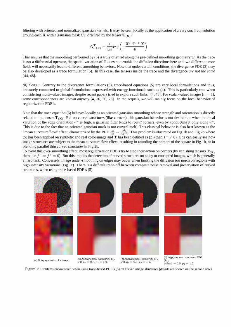
Note that the trace equation (5) behaves locally as an oriented gaussian smoothing whose strength and orientation is directlyrelated to the tensorT(X). But on curved structures (like corners), this gaussian behavior is not desirable : when the localvariation of the edge orientationθ− is high, a gaussian filter tends toround corners, even by conducting it only alongθ−.This is due to the fact that an oriented gaussian mask is not curved itself. This classical behavior is also best known as the“mean curvature flow” effect, characterized by the PDE∂I

∂t = ∂2I

∂θ−2 . This problem is illustrated on Fig.1b and Fig.2b where(5) has been applied on synthetic and real color image andT has been defined as (2) (thenf− 6= 0). One can easily see howimage structures are subject to the mean curvature flow effect, resulting in rounding the corners of the square in Fig.1b,or inblending parallel thin curved structures in Fig.2b.To avoid this over-smoothing effect, most regularization PDE’s try to stop their action on corners (by vanishing tensorsT(X)

there, i.ef− = f+ = 0). But this implies the detection of curved structures on noisy or corrupted images, which is generallya hard task. Conversely, image under-smoothing on edges mayoccur when limiting the diffusion too much on regions withhigh intensity variations (Fig.1c). There is a difficult trade-off between complete noise removal and preservation of curvedstructures, when using trace-based PDE’s (5).

(a) Noisy synthetic color image (b) Applying trace-based PDE (5),with p1 = 0.5, p2 = 1.2.

(c) Applying trace-based PDE (5),with p1 = 0.9, p2 = 1.2.

(d) Applying our constrained PDE(14),with p1 = 0.5, p2 = 1.2.

Figure 1:Problems encountered when using trace-based PDE’s (5) on curved image structures (details are shown on the second row).

(a) Image of a fingerprint(b) Applying trace-based PDE (5),with p1 = 0.5, p2 = 1.2.

(c) Applying our constrained PDE (14),with p1 = 0.5, p2 = 1.2.

Figure 2:Comparisons between trace-based PDE’s (5) and our new curvature-preserving PDE’s (14) on a real image.

Actually, this kind of regularization processes does not care about thecurvatureof the smoothing directions, and by extension,of the curvature of the image contours. Taking this curvature into account is a very desirable goal and has motivated the workpresented in the sequels : in section 3, we propose a new classof trace-based regularization PDE’s that smooth an imageI

along a tensor fieldT, while implicitly taking curvatures of specific integral curves ofT into account. Roughly speaking,we want to locally filter the image withcurved gaussian kernelswhen necessary, in order to better preserve image structures.For illustration purposes, results of our curvature-preserving equation is shown on Fig.1d and Fig.2c.*

3 Curvature-Preserving PDE’s

3.1 The single direction case

To illustrate the general idea of curvature-preserving PDE’s, we first focus on image regularization along avector fieldw : Ω → R

2 instead of a tensor fieldT. We consider then a local smoothing everywhere along a single direction w

‖w‖ , with

a smoothing strength‖w‖. We denote the two spatial components ofw by w(X) = (u(X) v(X))T .

We propose to define the followingcurvature-preservingregularization PDE that smoothesI alongw by :

∀i = 1, . . . , n,∂Ii∂t

= trace(

wwT

Hi

)

+ ∇ITi Jww (6)

whereJw stands for the Jacobian ofw , andHi is the Hessian ofIi.

Jw =

∂u∂x

∂u∂y

∂v∂x

∂v∂y

and Hi =

∂2Ii

∂x2∂2Ii

∂x∂y

∂2Ii

∂x∂y∂2Ii

∂y2

The PDE (6) adds a term∇ITi Jww to the trace-based equation (5) that smoothesI alongw with locally oriented gaussian

kernels (see section 2.3). This extra term naturally depends on the variation of the vector fieldw. Let us explain how (6) isrelated tow.

Let CX

(a) be the curve defining theintegral curveof w, starting fromX and parameterized bya ∈ R :

CX

(0) = X

∂CX

(a)

∂a = w(CX

(a))

(7)

Whena→ +∞ the integral curveCX

(a) is trackedforward, andbackwardwhena→ −∞ (Fig.3). We denote byF the familyof integral curves ofw.

(a) Integral curve of a general fieldw.(b) Example of integral curves whenw is the lowest eigenvector of thestructure tensorG of a color imageI (one block is one color pixel).

Figure 3: Integral curveCX of vector fieldsw : Ω → R2.

A second-order Taylor development ofCX

(a) arounda = 0 is :

CX

(h) = CX

(0) + h∂CX

(a)

∂a |a=0+h2

2

∂2CX

(a)

∂a2 |a=0+O(h3)

= X + hw(X) +h2

2Jw(X)

w(X) +O(h3)

with h → 0, andO(hn) = hn ǫn. Then, we can compute a second-order Taylor development ofIi(CX

(a)) arounda = 0,

which corresponds to the variations of the image intensity nearX when following the integral curveCX :

Ii(CX

(h)) = Ii

(

X + hw(X) +h2

2Jw(X)

w(X) +O(h3)

)

= Ii(X) + h∇IiT(X) (w(X) +h

2Jw(X)

w(X)) +h2

2trace

(

w(X)wT(X)Hi(X)

)

+O(h3)

The term trace(

w(X)wT(X)Hi(X)

)

= ∂2Ii

∂w2 corresponds to the second directional derivative ofIi alongw.

The second derivative of the functiona→ Ii(CX

(a)) ata = 0 is then :

∂2Ii(CX

(a))

∂a2 |a=0= lim

h→0

1

h2

[

Ii(CX

(h)) + Ii(CX

(−h)) − 2Ii(CX

(0))]

= limh→0

1

h2

[

h2 ∇ITi Jw(X)

w(X) + h2 trace(

w(X)wT(X)Hi(X)

)

+O(h3)]

= trace(

w(X)wT(X)Hi(X)

)

+ ∇ITi Jw(X)

w(X) (8)

Note that this is exactly the right term in our curvature-preserving PDE (6).

Actually, (6) can be seen individually for all integral curves ofF instead of each pointX ∈ Ω : consider another pointY ∈ CX. Then, there existǫ ∈ R such thatY = CX

(ǫ). Indeed,CX andCY describe the same curve (7) with different

parameterizations :∀a ∈ R, CY

(a) = CX

(ǫ+a). As (6) is verified onY, then∂Ii(CX

(a))

∂t |a=ǫ=

∂2Ii(CX

(a))

∂a2 |a=ǫ. This is obviously

true forǫ ∈ R since (6) is verified for all pointsY lying on the integral curveCX. Then, the PDE (6) may be also written as :

∀C ∈ F , ∀a ∈ R,∂Ii(C(a))

∂t=∂2Ii(C(a))

∂a2(9)

We recognize in (9) aone-dimensional heat flow constrained onC. This is actually very different from a heat-floworientedby w, as in the formulation∂Ii

∂t = ∂2Ii

∂w2 since the curvatures of integral curves ofw are now implicitly taken into account.In particular, our constrained equation has the interesting property to vanish when image intensities are perfectly constant onthe integral curveC, whatever the curvature ofC is. In this context, defining a fieldw that is tangent everywhere to the imagestructures will allow the preservation of these structures, even if they are curved (such as corners). This is not the case withdivergence or trace-based PDE’s (3),(5) classically used in image regularization. This curvature-preserving property of (6) isillustrated on Fig.1d and Fig.2b.Our constrained equation (6) is anelliptic PDE since the matrixww

T is positive definite. The existence and unicity of thesolutions of (6) are not directly approached in this article. Anyway, in next section 3.2, we show that its solution can beapproximated by the technique of line integral convolutions, which is a well-posed analytical approach.

3.2 Curvature-Preserving PDE’s and Line Integral Convolutions

Line Integral Convolutions (LIC) have been first introducedin [11] as a technique to render a textured imageILIC that

represents a vector fieldw : Ω → R2. The idea, originally expressed as a discrete form, consists in smoothing an image

Inoise - containing only noise - by averaging its pixel values alongthe integral curves ofw. Actually, a continuous formulation

of a LIC is then :

∀X ∈ Ω, ILIC(X) =

1

N

∫ +∞

−∞f(p) I

noise(CX

(p)) dp (10)

wheref : R → R is an even function (strictly decreasing to0 on R+) andCX is defined as theintegral curve(7) of

w throughX. The normalization factorN allows the preservation of the average pixel value alongCX and is equal toN =

∫ +∞−∞ f(p) dp.

As noticed in section 3.1, our curvature-preserving PDE (6)can be seen as the one-dimensional heat flow (9) constrained onthe integral curveCX ∈ F . Using the variable substitutionL(a) = I(CX

(a)), (9) can be also written as∂L

∂t (a) = L′′

(a). The

solutionL[t] at timet is known to be the convolution ofL[t=0] by a normalized gaussian kernelGt (see [20, 25]) :

L[t](a) =

∫ +∞

−∞L

[t=0](p) Gt(a−p) dp with Gt(p) =

1√4πt

exp

(

−p2

4t

)

(11)

SubstitutingL in (11) witha = 0, and remembering thatCX

(0) = X andGt(−p) = Gt(p) :

∀X ∈ Ω, I[t](X) =

∫ +∞

−∞I[t=0](CX

(p)) Gt(p) dp (12)

The equation (12) is a particular form of the continuous LIC-based formulation (10) with a gaussian weighting functionf = Gt. Here, the normalization factor isN =

∫ +∞−∞ Gt(p) dp = 1. Intuitively, the evolution of our curvature-preserving

PDE (6) may be seen as the application of local convolutions by normalized one-dimensional gaussian kernelsalong integralcurvesC of w. This kind of anisotropic image smoothing considers then acurvedfiltering, instead of just an oriented one.Applying this setting on a multi-valued imageI, with w being the lowest eigenvector of the structure tensor fieldG (i.e.the contour direction) allows the anisotropic smoothing ofI with edge preservation, even if these edges are curved. Thisis illustrated on Fig.3b, where few integral linesCX are computed, around a typical T-junction structure. Note how thestreamlines rotate when arriving at the junction, with a sub-pixel precision. The streamlines have been computed with a2nd-order Runge-Kutta scheme.

Note that (12) is an analytical solution of (6) whenw does not evolve over time. This property is generally not verifiedwhen dealing with general nonlinear regularization PDE’s,where the smoothing geometry is re-evaluated at each time step(this defines a temporal non-linearity). In order to get thiskind of non-linearity, we will then to perform several successiveiterations of our LIC scheme (12), where the vector fieldw is updated at each iteration. This is actually a good way of ap-proximating (6). Classical explicit schemes usually consider the smoothing geometryw as constant between two successivePDE iterationsI[t] andI[t+dt]. Thus, our curvature-preserving equation (6) will be efficiently discretized by several iterationsof our LIC formulation (12) (section 4).Note also that PDE-based algorithms performing vector flow visualization with textures have been already proposed in[6, 34], mainly inspired by the popular LIC technique, but notheoretical links between PDE-based formulations and LIC’shave been done. Moreover, the use of divergence-based equations proposed in these paper does not ensure the correctnessofthe smoothing directions, as pointed out in section 2.2.

3.3 Between Traces and Divergences

We illustrate here how our curvature-preserving PDE (6) maybe regarded compared to trace and divergence expressions (3),(5), for the case of single direction smoothingT = ww

T .In this case, the divergence PDE (3) may be developed as :

div(

wwT ∇Ii

)

= div

u2 ∂Ii

∂x + uv ∂Ii

∂y

uv ∂Ii

∂x + v2 ∂Ii

∂y

=

(

u2 ∂2Ii∂x2

+ 2uv∂2Ii∂x∂y

+ v2 ∂2Ii∂y2

)

+ ∇ITi

2u ∂u∂x + u ∂v

∂y + v ∂u∂y

2v ∂v∂y + u ∂v

∂x + v ∂u∂x

= trace(

wwTHi

)

+ ∇ITi

u ∂u∂x + v ∂u

∂y

u ∂v∂x + v ∂v

∂y

+

u ∂u∂x + u ∂v

∂y

v ∂u∂x + v ∂v

∂y

= trace(

wwTHi

)

+ ∇ITi Jww + div(w)∇IT

i w

Thus, we recognize in these three different terms :

• The first term corresponds to the trace PDE (5), that smootheslocally I alongw.

• The two first terms correspond to ourcurvature-constrainedregularization PDE (6), that smoothes locallyI alongw

while taking the curvature of integral curvesC of w into account.

• The three terms together correspond to the classical divergence PDE (3) that performs local diffusions ofI alongw. This last term div(w)∇IT

i w is mainly responsible for the perturbations of the effective smoothing direction, asdescribed in section 2.2. It is not desirable for image regularization purposes.

It is interesting to observe that our curvature-constrained PDE (6) is then “mathematically” positioned between the trace (5)and divergence formulations (3), and allows at the same timethe full respect of the pre-defined smoothing directionsw, whilepreserving curved images structures.Note that we can also write our curvature-preserving PDE (6)as a divergence-based PDE minus a constraint term :

trace(

wwTHi

)

+ ∇ITi Jww = div

(

wwT ∇Ii

)

− div(w)∇ITi w

Two particular cases of directionsw are worth studying, in the case of scalar-valued images (n = 1) :

• Whenw = ∇I⊥

‖∇I‖ (isophote direction), then ∇ITJww = −Iww, vanishing then the velocity of our curvature-

preserving evolution equation (6), by counterbalancing the trace-based term (which is nothing more than themean

curvature motionin this case). No smoothing will be then performed. This is quite natural since pixel along theisophotes have constant values, so averaging those values will not change the image. Note by comparison that thevelocity of the corresponding divergence-based expression div

(

wwT ∇Ii

)

also vanishes here.

• Whenw = ∇I‖∇I‖ (gradient direction), then ∇IT

Jww = 0, and the velocity of our curvature-preserving PDE (6)becomes simplyIww, which really corresponds to a smoothing of the image along the gradient direction (the same asthe unconstrained trace-based PDE (5)). Note by comparisonthat the velocity of the corresponding divergence-basedexpression is∆I in this case, which corresponds to an isotropic smoothing ofthe image, instead of an anisotropic one.

These two particular cases allows to better understand the difference of regularization behaviors between the trace, divergenceand curvature-preserving formulations.Note also that in case wherew is a divergence free field (i.e÷(w) = 0), the divergence-based PDE (3) and our curvature-preserving formulation (6) are strictly equivalent.

3.4 Extension to multi-directional smoothing

We extend our single-direction smoothing PDE (6) so that it can deal with a tensor-valued geometryT : Ω → P(2), insteadof a vector-valued geometryw. As pointed out in section 2.1, a diffusion tensor describesmuch more complex smoothingbehaviors than single directions. In particular, it may represents bothanisotropicor isotropic regularization behaviors. Theextension of our curvature-preserving PDE (6) is not straightforward : the notions of curvature and integral curves of tensors-valued fieldsT are not as natural as with direction fieldsw.To tackle this problem, we propose to locally decompose a tensor-driven smoothing process into several vector-drivensmoothing processes along different orientations. We firstnotice that

∫ π

α=0

aαaTα dα =

π

2Id where aα =

cosα

sinα

Then, any2 × 2 tensorT may be written as :

T =2

π

√T

(∫ π

α=0

aαaTα dα

)√T

where√

T =√

f+uuT +

√

f−vvT stands for the square root ofT = f+

uuT + f−

vvT . One can easily verify that

(√

T)2 = T and(√

T)T =√

T. Thus, the tensorT may be decomposed as :

T =2

π

∫ π

α=0

√Taαa

Tα

√T

Tdα

=2

π

∫ π

α=0

(√

Taα)(√

Taα)T dα (13)

We have split the tensorT into a sum ofatomic tensors(√

Taα)(√

Taα)T , each being purely anisotropic and directedonly along the direction of the vector

√Taα ∈ R

2. The equation (13) naturally suggests to decompose any tensor-drivenregularization PDE into a sum of single direction smoothingprocesses, each of them respecting the overall geometryT. Forinstance :

• If T = Id (identity matrix), the tensor is isotropic and :∀α ∈ [0, π],√

Taα = aα. The resulting smoothing will bethen performed in all directionsaα of the plane with the same strength.

• If T = uuT (whereu ∈ S1), the tensor is purely anisotropic and :∀α ∈ [0, π],

√Taα = (uT aα)u. The resulting

smoothing will be then performed only along the directionu of the tensorT.

Then, using (13) and considering that each single directionsmoothing must be done with a curvature-preserving approach

(6), we propose the following constrained regularization PDE, acting on a multi-valued imageI : Ω → Rn and driven by a

tensor-valued smoothing geometryT :

∀i = 1, . . . , n,∂Ii∂t

=2

π

∫ π

α=0

trace(

(√

Taα)(√

Taα)THi

)

+ ∇ITi J√

Taα

√Taα dα

which can be simplified as :

∀i = 1, . . . , n,∂Ii∂t

= trace(THi) +2

π∇IT

i

∫ π

α=0

J√Taα

√Taα dα (14)

whereaα = (cosα sinα)T , andJ√Taα

stands for the Jacobian of the vector fieldΩ →√

Taα. Note that this kind ofsmoothing decomposition along all orientations of the plane can be also found in [51]. As in the single direction smoothingcase, (14) may be seen as a trace-based equation (5), where anextra term has been added in order to respect the curvature ofall integral lines passing through the tensor-valued geometry T.

4 Implementation considerations

In order to implement our regularization method (14), we benefit from the LIC-based intepretation of curvature-preservingPDE’s presented in section 3.2. Indeed, we can explicitely discretize (14) by the following Euler scheme :

I[t+dt] = I

[t] +2dt

N

(

N−1∑

k=0

R(√

Taα)

)

whereα = kπ/N (in the interval[0, π]), dt is the usual temporal discretization step andR(w) represents a discretization ofthe mono-directional smoothing PDE velocity (6) that preserve curvatures along a vector fieldw. If we write this expression

as :I[t+dt] = 1N

(

∑N−1k=0 I

[t] + 2dt R(√

Taα))

, we may express it as the averaging of different gaussian-ponderated LIC’s

along vector fields√

Taα :

I[t+dt] =

1

N

(

N−1∑

k=0

I[t]

LIC(√

Taα)

)

,

where each gaussian variance has a standard deviationdt.Basically, the difficulty here is the LIC computation, whichneeds the tracking of integral curves of a vector field. Here,weused a very simple method based on the classical Runge-Kutta[35] integration scheme. Faster LIC implementations havebeen proposed in [40] but do not deal with gaussian ponderation functions, as needed here.This simple observation leads then to the following fast algorithm for the implementation of one iteration of our curvature-preserving PDE (14) :

1. Compute the smoothed structure tensor fieldGσ from I[t] :

Gσ = Gσ ∗n∑

i=1

(

∂I[t]i

∂x

)2 (

∂I[t]i

∂x

)(

∂I[t]i

∂y

)

(

∂I[t]i

∂x

)(

∂I[t]i

∂y

) (

∂I[t]i

∂y

)2

σ will depend on the noise scale. We used relatively low values(between0 and1.5) for our experiments in section 5.

2. Compute the eigenvaluesλ+, λ− and eigenvectorsθ+, θ− of Gσ.

3. Compute the smoothing geometry tensor fieldT from Gσ : T = 1(1+λ++λ−)p1

θ−θ−T

+ 1(1+λ++λ−)p2

θ+θ+T

4. For allα in [0, π] (discretized with a user-fixed stepdα) :

• Compute the vector fieldw =√

T aα.

• Perform a Line Integral Convolution ofI[t] alongCX in the forward and backward directions.

5. Average all LIC’s computed in step 4.

The main parameters of our algorithm arep1, p2, σ, dt and the number of PDE iterationsnb that are applied. The character-istics of this scheme, compared to the classical finite-difference one is :

• It allows the preservation of thin image structures from a numerical point of view : the smoothing is performed alongintegral curves ofw, with a sub-pixel accuracy. Precise Runger-Kutta interpolation is used to track the integral curvesC.

• It allows to choose very large time stepsdt, since the scheme we proposed is unconditionally stable. Indeed,dt simplycorresponds to a smoothing variance of the gaussian-ponderated convolution alongC ∈ F .

• As a result, the regularization algorithm performs very fast. Very few iterations are necessary to get the result, evenif each iteration is more time-consuming. For our applications, presented in section 5, we were even able to choosenb = 1 iteration with very large time stepsdt. In fact, this leads to a rough approximation of (14), since we lost thetemporal non-linearity property of the PDE. But for images with few noise, this gave suprisingly good results. Actually,the spatial non-linearity seems to play a more important role than the temporal non-linearity in our scheme.

The smoothing is done as an averaging of multiple LIC’s in different directionsα. The choice of the discretization stepdα

is important in this context. Actually, in regions where thesmoothing needs to be mostly anisotropic, only few values ofαare necessary since in all cases, the smoothing will be done along the same single direction. But in homogeneous regionsneeding isotropic smoothing, a smallerdα will give much better results. Practically speaking, we chosedα = 45o which isenough to get a good precision for isotropic smoothing.On Fig.4, we illustrate the efficiency of our new scheme, compared to the classical finite-difference one. A synthetic noisyimage is anisotropically smoothed with our PDE (14), withp1 = 0.01 andp2 = 100 (smoothing mostly along isophotesθ−,with a strength of1). The LIC-based scheme (Fig.4c) better preserves the structure along timet. This is due to the importantrole played by the sub-pixel accuracy property of the underlying LIC computation.

(a) Noisy color image.(b) Regularization using a finite-difference scheme(stopped att = 100).

(c) Regularization using our LIC-based scheme(stopped att = 100).

Figure 4: Comparisons between classical explicit PDE schemes, and LIC-based implementation of our PDE (14).

5 Application Results

We present different application results of our curvature-preserving PDE (14), implemented by the LIC-based scheme andapplied on24bits color imagesI : Ω → [0, 255]3. The(R,G,B) color base has been considered for the PDE evolutions.All experiments have been performed on a PC2.8 Ghz running Linux (single CPU). The implementation has beendone inC++, thanks tothe CImg Library[49], a very simple-to-use and powerful image processing library. For each result presentedbelow, we detail the used parameters and the processing time.

5.1 Color Image Denoising and Regularization

Image denoising is a direct application of regularization methods. Sensor inaccuracies, digital quantifications or compressionartefacts are indeed some of the various noise sources that can affect a digital image, and suppressing them is a desirablegoal. In Fig.5, we illustrate how our curvature-preservingPDE (14) can be successfully applied to remove such artefactswhile preserving the essential structures of the processedimages.

• Fig.5a shows a restoration of the “baboon” color image, artificially degraded by adding uncorrelated gaussian noise on(R,G,B). This512× 512 color image has been regularized with (14) and a140× 111 portion of the image is shown.Only one PDE iteration has been necessary, withp1 = 0.5, p2 = 0.7, σ = 1.5 anddt = 50. Processing time is19.3seconds for the entire image.

• Fig.5b illustrates a real case where a color photograph has been digitized from a grainy paper, leading to the apparitionof watered effects on the digital picture (size=586 × 367). Using our regularization method allows to clearly removethe grain while preserving quite fine structures (palm tree leafs). Shown image is a152 × 133 portion of the originalone. Only one PDE iteration has been necessary, withp1 = 0.5, p2 = 0.7, σ = 1 anddt = 10. Processing time is11seconds for the entire image.

• Fig.5c deals with the suppression of compression artefactsin color images. A JPEG version of the “Lena” color image(size=256×256, where the JPEG quality ratio has been set to10%) is processed by our regularization algorithm. Usualblock effects inherent to the DCT compression are visible onthe compressed image (left). One PDE iteration is appliedthen, withp1 = 0.5, p2 = 0.9, σ = 2, dt = 200, in order to get the regularized result (right). Only a100 × 73 portionof the original image is shown. Processing time is6.4 seconds for the entire image.

• Fig.5d illustrates how our regularization method is used toimprove a digital color image quantified in256 colors bythe Floyd-Steinberg algorithm (size=355× 287). One PDE iteration has been applied, withp1 = 0.5, p2 = 0.8, σ = 1,dt = 30. A 136 × 118 portion of the image is shown. Processing time is12.8 seconds for the entire image.

• Fig.5e shows a digital photograph shot under low luminosityconditions, leading to the apparition of real digital noise(poisson noise). Processed color image has size=293 × 306 and has been restored in5.6 seconds (one PDE iteration),with parametersp1 = 0.2, p2 = 0.5, σ = 2, dt = 120.

• Fig.5f illustrates how exaggerating the smoothing geometry can create interesting painting effects. One PDE iterationof (14) has been applied, withp1 = 0.5, p2 = 1.2, σ = 4 (which leads to an exaggeratedly smooth geometryT) anddt = 20. Processing time is26 seconds for this460 × 365 color image.

Note that our equation (14) is acting a as intelligent image smoother. It is actually not able to perform edge enhancement, asdivergence-based PDE’s (3) may do. This would be possible anyway by adding a classical shock-filter term (such as proposedin [2, 31] for scalar images and extended in [44, 55] for multi-valued ones) to our curvature-preserving PDE formulation(14).Generally, this enhancement is not necessary for noisy images, particularly since we preserve the edges very well with ourcurvature-preserving method.

5.2 Color Image Inpainting

Image inpainting is a very new and challenging application,which consists in filling-in missing (user-defined) image regionsby guessing pixel values such that the reconstructed image still looks natural. Basically, the user provides one color imageI : Ω → R

3, and onemaskimageM : Ω → 0, 1. The inpainting algorithm must fill-in the regions whereM(X) = 1,by the mean of some intelligent interpolations. Inpaintingalgorithms can be used for instance to remove various structuresin images (scratches, logos or real objects). Pioneering work on image inpainting has been first proposed as a variationalformulation by Masnou and Morel [29], followed by many PDE-based solutions [8, 9, 15, 48]. It is also worth to cite somepapers related to inpainting without use of PDE’s [19, 22], among others.In this article, we see the inpainting process as a direct application of our proposed curvature-preserving PDE (14). Applyingthe diffusion equation only on the regions to inpaint allowsthe neighbor pixels to diffuse inside these regions : a nonlinearcompletion of the image data along isophotes directions is thus naturally done, reconstructing the missing parts of theimage.This kind of PDE-based inpainting technique has been also proposed in [8, 15, 48]. Note that it is not able to perform texturereconstructions, and texture synthesis steps will be sometimes necessary [3, 9, 56].

(a) Denoising of the “baboon” color image (19.3s).

(b) Watered effect suppression in a color image (11s).

(c) Suppression of JPEG compression artefacts in the “lena”image (6.4s). (d) Suppression of quantification artefacts in a 8bits color image (12.8s).

(e) Denoising of a digital photograph with digital noise (5.6s). (f) Creating painting effects with over-smoothing procedures (26s).

Figure 5: Results of color image regularization using our curvature-preserving PDE’s (14).

(a) Inpainting a cage (middle) in a color image (left). Inpainted in 4m11s (right).

(b) Removing subtitles from a movie frame (11s).

(c) Left : Zoom of (b). Right : Reconstruction of a color image where50% of the pixel values have been suppressed (1m01s).

Figure 6: Results of color image inpainting using our curvature-preserving PDE (14).

• Fig.6a shows how our PDE-based inpainting technique can be used to remove real objects from digital photographs. A500× 500 color image (left) is inpainted with a user-defined mask (middle). The inpainted image (right) is obtained in4 minutes11 seconds, after200 iterations of our PDE (14) with parametersp1 = 0.001, p2 = 100, σ = 4, dt = 150.Note thatp1 << p2 encourages smoothing only along the isophote directions with a strength of 1 everywhere.

• Fig.6b shows an application of subtitles removing in a movieframe. Image size is300 × 162 and the inpainted imagehas been obtained after20 iterations of (14), withp1 = 0.001, p2 = 100, σ = 4, dt = 50, for a total processing timeof 11 seconds.

• Fig.6c illustrates the reconstruction capabilities of ourinpainting technique. Half of the pixels of a300 × 246 colorimage have been suppressed by masking them with a16 × 16 checkerboard-shaped mask. Then, the image is recon-structed using10 iterations of our PDE (14) inside the inpainting mask, with parametersp1 = 0.001, p2 = 100, σ = 4anddt = 50 (processing time is1 minute01 seconds).

For each inpainting result shown in this article, the initialization of the pixel values inside the inpainting masks att = 0 hasbeen done by white noise. Actually, the inpainting algorithm is not much dependent of the initialization step : the equation(14) diffuses neighborhood values inside the inpainting mask until convergence, and there is then a strong border condition.We didn’t see much difference between different types of initialization (noise, zero-filling or linear interpolation).

(a) Original color image

Figure 7: Comparisons of image resizing, using Nearest-neighbor (first row), Linear (second row), Bicubic (third row) andPDE-based (last row) interpolations.

5.3 Color Image Resizing

The inpainting technique naturally suggests that the nonlinear interpolation implicitly performed by our regularization PDE(14) can be also applied to magnify images, just as a replacement to classical linear or bicubic interpolations. This is doneas follows : starting from a linear or bicubic magnification of a color image as an initialization, we apply our curvature-preserving PDE (14) everywhere except on the pixels having “known” intensity values (pixels created from the originalimage points). This is actually very similar to image inpainting with a very sparse grid for the mask.

• Fig.7 illustrates one example of image resizing. An original 220 × 210 color image is resized by a factor×2 withclassical nearest-neighbor, linear and bicubic interpolations, then by our PDE-based technique (14). Our non-linearregularization filter allows to remove the aliasing effectsusually encountered with simple interpolation methods, whilecorrectly preserving the edges of the image.

Notice that we always preserve the values of the points corresponding to the original thumbnail image, so that resizing backthe image to its original dimension (sub-sampling) resultsin the original input data.

5.4 Other Results & Availability

Many application results of our algorithm can be found at thefollowing web page :

http://www.greyc.ensicaen.fr/˜dtschump/greycstorati on/

You can also download and test the algorithm on different architectures. Finally, the source of the algorithm (in C++) isavailable as a part of the open sourceCImg Library[49].

Conclusion

We proposed a generic constrained regularization formalism able to anisotropically smooth multi-valued images with PDE’swhile preserving natural curvature constraints. It can be used in a wide range of image processing applications, includingimage denoising, inpainting, interpolation among others.This formalism makes the link between general diffusion PDE’s andLine Integral Convolutions, and leads to the design of a veryfast and efficient numerical scheme that implements the method.This may ease the introduction of nonlinear diffusion methods for time-critical applications in the area of multimedia, medicalimaging and image processing in general.

References

[1] L. Alvarez, F. Guichard, P.L. Lions, and J.M. Morel.Axioms and fundamental equations of image processing.Archivefor Rational Mechanics and Analysis, Vol.123, No.3, pp.199–257, 1993.

[2] L. Alvarez and L. Mazorra.Signal and Image Restoration using Shock Filters and Anisotropic Diffusion.SIAM Journalof Numerical Analysis, Vol.31, No.2, pp.590–605, 1994.

[3] M. Ashikhmin. Synthesizing Natural Textures. ACM Symposium on Interactive 3D Graphics, Research Triangle Park,NorthCarolina, pp.217–226, March 2001.

[4] G. Aubert and P. Kornprobst.Mathematical Problems in Image Processing: Partial Differential Equations and theCalculus of Variations, Applied Mathematical Sciences, Vol.147, Springer-Verlag, January 2002.

[5] D. Barash.A Fundamental Relationship between Bilateral Filtering, Adaptive Smoothing and the Nonlinear DiffusionEquation.IEEE Transactions on Pattern Analysis and Machine Intelligence, Vol.24, No.6, p.844.

[6] J. Becker, T. Preusser, and M. Rumpf.PDE methods in flow simulation post processing.Computing and Visualization inScience, Vol.3, No.3, pp.159–167, 2000.

[7] M. Bertalmio, L.T. Cheng, S. Osher, and G. Sapiro.Variational Problems and Partial Differential Equations on ImplicitSurfaces.Computing and Visualization in Science, Vol.174, No.2, pp.759–780, 2001.

[8] M. Bertalmio, G. Sapiro, V. Caselles, and C. Ballester.Image inpainting.ACM SIGGRAPH, International Conferenceon Computer Graphics and Interactive Techniques, pp.417–424, 2000.

[9] M. Bertalmio, L. Vese, G. Sapiro, and S. Osher.Simultaneous Structure and Texture Image Inpainting. IEEE Transactionson Image Processing, Vol.12, No.8, pp.882–889, August 2003.

[10] M.J. Black, G. Sapiro, D.H. Marimont, and D. Heeger.Robust anisotropic diffusion.IEEE Transaction on ImageProcessing, Vol.7, No.3, pp.421–432, 1998.

[11] B. Cabral and L.C. Leedom.Imaging vector fields using line integral convolution.SIGGRAPH’93, in ComputerGraphics Vol.27, pp.263–272, 1993.

[12] R. Carmona and S. Zhong.Adaptive Smoothing Respecting Feature Directions.IEEE Transactions on Image Processing,Vol.7, No.3, pp.353–358, 1998.

[13] A. Chambolle and P.L. Lions.Image recovery via total variation minimization and related problems. NumerischeMathematik, Vol.76, No.2, pp.167–188, 1997.

[14] T. Chan and J. Shen.Variational restoration of non-flat image features : Modelsand algorithms.SIAM Journal ofApplied Mathematics, Vol.61, No.4, pp.1338–1361, 2000.

[15] T. Chan and J. Shen.Non-texture inpaintings by curvature-driven diffusions.Journal of Visual Communication andImage Representation, Vol.12, No.4, pp.436–449, 2001.

[16] P. Charbonnier, L. Blanc-Feraud, G. Aubert, and M. Barlaud.Deterministic edge-preserving regularization in computedimaging. IEEE Transactions on Image Processing, Vol.6, No.2, pp.298–311, 1997.

[17] C. Chefd’hotel, D. Tschumperle, R. Deriche, and O. Faugeras. Regularizing Flows for Constrained Matrix-ValuedImages.Journal of Mathematical Imaging and Vision, Vol.20, No.2, pp.147-162, January 2004.

[18] O. Coulon, D.C. Alexander, and S.R. Arridge.A regularization scheme for diffusion tensor magnetic resonance images.17th International Conference on Information Processing in Medical Imaging, LNCS, Vol.2082, pp.92–105, 2001.

[19] A. Criminisi, P. Perez, and K. Toyama.Object Removal by Exemplar-based InpaintingIEEE Conference on ComputerVision and Pattern Recognition, Vol.2, pp.721–728, June 2003.

[20] R. Deriche and O. Faugeras.Les EDP en traitement des images et vision par ordinateur.Traitement du Signal, Vol.13,No.6, 1997.

[21] S. Di Zenzo A note on the gradient of a multi-image.Computer Vision, Graphics and Image Processing, Vol.33,pp.116-125, 1986.

[22] J. Jia and C.K. TangImage Repairing : Robust Image Synthesis by AdaptiveND Tensor VotingIEEE Conference onComputer Vision and Pattern Recognition, Vol.1, pp.643–650, June 2003.

[23] R. Kimmel, R. Malladi, and N. Sochen.Images as embedded maps and minimal surfaces: movies, color, texture, andvolumetric medical images.International Journal of Computer Vision, Vol.39, No.2, pp.111–129, September 2000.

[24] R. Kimmel and N. Sochen.Orientation diffusion or how to comb a porcupine.Journal of Visual Communication andImage Representation, Vol.13, pp.238–248, 2002.

[25] J.J. Koenderink.The structure of images.Biological Cybernetics, Vol.50, pp.363–370, 1984.

[26] P. Kornprobst, R. Deriche, and G. Aubert.Nonlinear operators in image restorationIEEE Conference on ComputerVision and Pattern Recognition, pp 325-331, June 1997.

[27] K. Krissian. Multiscale Analysis : Application to Medical Imaging and 3DVessel Detection.Ph.D. Thesis, INRIA-Sophia Antipolis/France, 2000.

[28] T. Lindeberg.Scale-Space Theory in Computer Vision. Kluwer Academic Publishers, 1994.

[29] S. Masnou and J-M. Morel.Level Lines Based Disocclusion.IEEE International Conference on Image Processing,Vol.3, pp.259-263, October 1998.

[30] M. Nielsen, L. Florack, and R. Deriche.Regularization, scale-space and edge detection filters.Journal of MathematicalImaging and Vision, Vol.7, No.4, pp.291–308, 1997.

[31] S. Osher and L.I. Rudin.Feature-oriented image enhancement using shock filters.SIAM Journal of Numerical Analysis,Vol.27, No.4, pp.919–940, August 1990.

[32] P. Perona.Orientation diffusions.IEEE Transactions on Image Processing, Vol.7, No.3, pp.457–467, March 1998.

[33] P. Perona and J. Malik.Scale-space and edge detection using anisotropic diffusion. IEEE Transactions on PatternAnalysis and Machine Intelligence, Vol.12, No.7, pp.629–639, July 1990.

[34] T. Preusser and M. Rumpf.Anisotropic nonlinear diffusion in flow visualization.IEEE Visualization Conference, 1999.

[35] W.H. Press, B.P. Flannery, S.A. Teukolsky, and W.T. Vetterling. “Runge-Kutta Method” in Numerical Recipes inFORTRAN: The Art of Scientific Computing, Cambridge University Press, pp. 704-716, 1992.

[36] L. Rudin, S. Osher, and E. Fatemi.Nonlinear total variation based noise removal algorithms.Physica D, Vol.60,pp.259–268, 1992.

[37] G. Sapiro.Geometric Partial Differential Equations and Image Analysis. Cambridge University Press, 2001.

[38] G. Sapiro and D.L. Ringach.Anisotropic diffusion of multi-valued images with applications to color filtering. IEEETransactions on Image Processing, Vol.5, No.11, pp.1582–1585, 1996.

[39] N. Sochen, R. Kimmel, and A.M. Bruckstein.Diffusions and confusions in signal and image processing.Journal ofMathematical Imaging and Vision, Vol.14, No.3, pp.195–209, 2001.

[40] D. Stalling and H.C. Hege.Fast and Resolution Independent Line Integral Convolution. ACM SIGGRAPH, 22ndAnnual Conference on Computer Graphics and Interactive Technique, pp.249–256, 1995.

[41] B. Tang, G. Sapiro, and V. Caselles.Direction diffusion.IEEE International Conference on Computer Vision, pp.1245,1999.

[42] B. Tang, G. Sapiro, and V. Caselles.Diffusion of general data on non-flat manifolds via harmonicmaps theory : Thedirection diffusion case.International Journal of Computer Vision, Vol.36, No.2, pp.149–161, February 2000.

[43] C. Tomasi and R. Manduchi.Bilateral filtering for gray and color images.IEEE International Conference on ComputerVision, pp.839–846, January 1998.

[44] D. TschumperlePDE’s Based Regularization of Multi-valued Images and Applications. PhD Thesis, Universite deNice-Sophia Antipolis/France, December 2002.

[45] D. Tschumperle and R. Deriche.Orthonormal Vector Sets Regularization with PDE’s and Applications. InternationalJournal of Computer Vision, Vol.50, pp. 237–252, 2002.

[46] D. Tschumperle and R. Deriche.Diffusion tensor regularization with constraints preservation. IEEE Conference onComputer Vision and Pattern Recognition, Vol.1, pp.948-953, December 2001.

[47] D. Tschumperle and R. DericheDiffusion PDE’s on Vector-Valued Images : Local Approach and Geometric Viewpoint.IEEE Signal Processing Magazine, Vol.19, No.5, pp.16–25, September 2002.

[48] D. Tschumperle and R. DericheVector-Valued Image Regularization with PDE’s : A Common Framework for DifferentApplications.IEEE Transactions on Pattern Analysis and Machine Intelligence, Vol.27, No.4, April 2005.

[49] D. Tschumperle.The CImg Library :http://cimg.sourceforge.net . The C++ Template Image ProcessingLibrary.

[50] B. Vemuri, Y. Chen, M. Rao, T. McGraw, T. Mareci, and Z. Wang. Fiber tract mapping from diffusion tensor MRI.IEEE Workshop on Variational and Level Set Methods in Computer Vision, July 2001.

[51] J. Weickert.Anisotropic Diffusion Filters for Image Processing Based Quality Control. 7th European Conference onMathematics in Industry, pp.355–362, 1994.

[52] J. Weickert.Anisotropic Diffusion in Image Processing. Teubner-Verlag, Stuttgart, 1998.

[53] J. Weickert. Coherence-Enhancing Diffusion of Colour Images. Image and Vision Computing, Vol.17, pp.199–210,1999.

[54] J. Weickert and T. Brox.Diffusion and Regularization of Vector and Matrix-valued Images.Inverse Problems, ImageAnalysis, and Medical Imaging, Vol.313 of Contemporary Mathematics, pp.251–268, 2002.

[55] J. Weickert Coherence-Enhancing Shock Filters.Pattern Recognition, 25th DAGM Symposium, LNCS, Vol.2781,pp.1–8, 2003.

[56] L.Y Wei and M. LevoyFast Texture Synthesis using Tree-structured Vector Quantization. ACM SIGGRAPH, Interna-tional Conference on Computer Graphics and Interactive Techniques, pp.479–488, 2000.