Fast Compaction Algorithms for NoSQL Databases

Mainak Ghosh, Indranil Gupta, Shalmoli GuptaDepartment of Computer Science

University of Illinois, Urbana ChampaignEmail: {mghosh4, indy, sgupta49}@illinois.edu

Nirman KumarDepartment of Computer Science

University of California, Santa BarbaraEmail: nirman@cs.ucsb.edu

Abstract—Compaction plays a crucial role in NoSQL systemsto ensure a high overall read throughput. In this work, weformally define compaction as an optimization problem thatattempts to minimize disk I/O. We prove this problem to be NP-Hard. We then propose a set of algorithms and mathematicallyanalyze upper bounds on worst-case cost. We evaluate theproposed algorithms on real-life workloads. Our results showthat our algorithms incur low I/O costs compared to optimaland that a compaction approach using a balanced tree is mostpreferable.

1. Introduction

Distributed NoSQL storage systems are being increas-ingly adopted for a wide variety of applications like onlineshopping, content management, education, finance etc. Fastread/write performance makes them an attractive option forbuilding efficient back-end systems.

Supporting fast reads and writes simultaneously on alarge database can be quite challenging in practice [13],[19]. Since today’s workloads are write-heavy, many NoSQLdatabases [2], [4], [11], [21] choose to optimize writes overreads. Figure 1 shows a typical write path at a server. Agiven server stores multiple keys. At that server, writes arequickly logged (via appends) to an in-memory data structurecalled a memtable. When the memtable becomes old orlarge, its contents are sorted by key and flushed to disk.This resulting table, stored on disk, is called an sstable.

Figure 1: Schematic representation of a typical writeoperations. Dashed box represents a memtable. Solid boxrepresents a sstable. Dashed arrow represents flushingof memory to disk.

This paper was supported in part by the following grants: NSF CNS1319527, NSF CCF 0964471, AFOSR/AFRL FA8750-11-2-0084, NSF CCF1319376, NSF CCF 1217462, NSF CCF 1161495 and a DARPA grant.

Figure 2: A compaction operation merge sorts multiplesstables into one sstable.

Over time, at a server, multiple sstables get generated.Thus, a typical read path may contact multiple sstables,making disk I/O a bottleneck for reads. As a result, readsare slower than writes in NoSQL databases. To make readsfaster, NoSQL systems periodically run a compaction proto-col in the background. Compaction merges multiple sstablesinto a single sstable by merge-sorting the keys. Figure 2illustrates an example.

In order to minimally affect normal database CRUD(create, read, update, delete) operations, sstables are mergedin iterations. A compaction strategy identifies the best candi-date sstables to merge during each iteration. To improve readlatency, an efficient compaction strategy needs to minimizethe compaction running time. Compaction is I/O-boundbecause sstables need to be read from and written to disk.Thus, to reduce the compaction running time, an optimalcompaction strategy should minimize the amount of diskbound data. For the rest of the paper, we will use the term“disk I/O” to refer to this amount of data. We consider thestatic version of the problem, i.e., the sstables do not changewhile compaction is in progress.

In this paper, we formulate this compaction strategy asan optimization problem. Given a collection of n sstables,S1

,. . .,Sn, which contain keys from a set, U , a compactionstrategy creates a merge schedule. A merge schedule defines

a sequence of sstable merge operations that reduces theinitial n sstables into one final sstable containing all keys inU . Each merge operation reads atmost k sstables from diskand writes the merged sstable back to disk (k is fixed andgiven). The total disk I/O cost for a single merge operationis thus equal to the sum of the size of the input sstables (thatare read from disk) and the merged sstable (that is writtento disk). The total cost of a merge schedule is the sum ofthe cost over all the merge operations in the schedule. Anoptimal merge schedule minimizes this cost.

Our Contribution. In this paper, we thoroughly study thecompaction problem from a theoretical perspective. We for-malize the compaction problem as an optimization problem.We further show a generalization of the problem whichcan model a wide class of compaction cost functions. Ourcontributions are as follows:• We prove that the optimization problem is NP-hard (Sec-

tion 3).• We propose a set of greedy algorithms for the compaction

problem with provable approximation guarantees (Sec-tion 4).

• We quantitatively evaluate the greedy algorithms withreal-life workloads using our implementation (Section 5).

Related Work. Bigtable [15] was among the first systems toimplement compaction. This system merges sstables whenthe number of sstables reaches a pre-defined threshold. Theydo not optimize for disk I/O. When the workload is read-heavy, running compaction over multiple iterations is slow inachieving the desired read throughput. To solve this, Level-based compaction [7], [9] merges every insert, updates anddeletes instead. Thus they optimize for reads by sacrificingwrites. NoSQL databases like Cassandra [1] and Riak [10]implement both these strategies [8], [12]. Cassandra’s Size-Tiered compaction strategy [12], inspired from Google’sBigtable, merges sstables of equal size. This approach bearsresemblance to our SMALLESTINPUT heuristic defined inSection 4. For data which becomes immutable over time,such as logs, specific compaction strategies have been pro-posed [3], [25] which look to prioritize compaction forrecent data as they are read more often. The goals of thesestrategies are orthogonal to ours. Outside ours, Mathieu et.al. [24] have also theoretically analyzed the compactionproblem. In their cost function, they optimize for CPU loadwhich is proportional to the sum of the cardinality of thesstables they merge in a iteration. Their merge scheduledetermines the number of sstables to merge in a iteration.Even though we optimize for different resources, it wouldbe worthwhile to compare our strategies. We plan to do thisin the future.

2. Problem Definition

Consider the compaction problem on n sstables for thecase where k = 2, i.e., in each iteration, 2 sstables aremerged into one. As we discussed in Section 1, an sstableconsists of multiple entries, where each entry has a key

and associated values. When 2 sstables are merged, thenew sstable is created which contains only one entry perkey present in either of the two base sstables. To give atheoretical formulation for the problem, we assume that: 1)all key-value pairs are of the same size, and 2) the valueis comprehensive, i.e., contains all columns associated witha key. This makes the size of an sstable proportional tothe number of keys it contains. Thus an sstable can beconsidered as a set of keys and a merge operation on sstablesperforms simple union of sets (where each sstable is a set).With this intuition, we can model the compaction problemfor k = 2 as the following optimization problem.

Given a ground set U = {e1

, . . . em} of m elements,and a collection of n sets (sstables), A

1

, . . . , An where eachAi ✓ U , the goal is to come up with an optimal mergeschedule. A merge schedule is an ordered sequence of setunion operations that reduces the initial collection of setsto a single set. Consider the collection of sets, initiallyA

1

, . . . , An. At each step we merge two sets (input sets) inthe collection, where a merge operation consists of removingthe two sets from the collection, and adding their union(output set) to the collection. The cost of a single mergeoperation is equal to the sum of the sizes of the two inputsets plus the size of the output set in that step. With n initialsets there need to be (n � 1) merge operations in a mergeschedule, and the total cost of the merge schedule is the sumof the costs of its constituent merge operations.

Observe that any merge schedule with k = 2 createsa full1 binary tree T with n leaves. Each leaf node in thetree corresponds to some initial set Ai, each internal nodecorresponds to the union of the sets at the two children, andthe root node corresponds to the final set. We assume thatthe leaves of T are numbered 1, . . . , n in some canonicalfashion, for example using an in-order traversal. Thus amerge schedule can be viewed as a full binary tree T withn leaves, and a permutation ⇡ : [n] ! [n] that assigns setAi (for 1 i n), to the leaf numbered ⇡(i). We callthis the merge tree. Once the merge tree is fixed, the setscorresponding to the internal nodes are also well defined.We label each node by the set corresponding to that node.By doing a bottom-up traversal one can label each internalnode. Let ⌫ be an internal node of such a tree and A⌫ beits label. For simplicity, we will use the term size of node⌫, to denote the cardinality of A⌫ .

In our cost function the size of a leaf node or the rootnode is counted only once. However, for an internal node(non-leaf, non-root node) it is counted twice, once as input,and once as output. Let V 0 be the set of internal nodes.Formally, we define the cost of the merge schedule as:

costactual(T,⇡, A1

, . . . , An) =

X

⌫2V 0

2 |A⌫ |+nX

i=1

|Ai|+ |Aroot|

Then, the problem of computing the optimal merge sched-ule is to create a full binary tree T with n leaves, andan assignment ⇡ of sets to the leaf nodes such that

1. A binary tree is full if every non-leaf node has two children

costactual(T,⇡, A1

, . . . , An) is minimized. This cost func-tion can be further simplified as follows:

cost(T,⇡, A1

, . . . , An) =

X

⌫2T

|A⌫ | (2.1)

The optimization problems over the two cost functionsare equivalent because the size of the leaf nodes, and theroot node is constant for a given instance. Further, an ↵-approximation for cost(T,⇡, A

1

, . . . , An) immediately givesa 2 · ↵-approximation for costactual(T,⇡, A1

, . . . , An). Forease of exposition, we use the simplified cost functionin equation (2.1) for all the theoretical analysis presentedin this paper. We call this optimization problem as theBINARYMERGING problem. We denote the optimal cost byopts(A1

, . . . , An).

A Reformulation of the Cost. A useful way to reformulatethe cost function cost(T,⇡, A

1

, . . . , An) is to count the costper element of U . Since the cost of each internal node isjust the size of the set that labels the node, we can say thatthe cost receives a contribution of 1 from an element at anode if it appears in the set labeling that node. The cost cannow be reformulated in the following manner. For a givenelement x 2 U , let T (x) denote the minimal subtree of Tthat spans all the nodes ⌫ in T whose label sets ⇡(⌫) containx and the root node. Let |T (x)| denote the number of edgesin T (x). Then we have that:

cost(T,⇡, A1

, . . . , An) =

X

x2U

(|T (x)|+ 1). (2.2)

Relation to the problem of Huffman Coding. We canview the problem of Huffman coding as a special case ofthe BINARYMERGING problem. Suppose we have n disjointsets A

1

, . . . , An with sizes |Ai| = pi. We can see that,using the full binary tree view and the reformulated costin equation (2.2), the cost function is the same as theproblem of an optimal prefix free code on n characters withfrequencies p

1

, . . . , pn.

Generalization of BINARYMERGING. As we saw, BI-NARYMERGING models a special case of the compactionproblem where in each iteration 2 sstables are merged.However in the more general case, one may merge atmostk sstables in each iteration. To model this, we introducea natural generalization of the BINARYMERGING problemcalled the K-WAYMERGING problem. Formally, given acollection of n sets, A

1

, . . . , An, covering a groundset Uof m elements, and a parameter k, the goal is to merge thesets into a single set, such that at each step: 1) atmost k setsare merged and 2) the merge cost is minimized. The costfunction is defined similar to BINARYMERGING.

Extension to Submodular Cost Function. In BINA-RYMERGING, we defined the cost of a merge operationas the cardinality of the set created in that merge step.However, in real-world situation the merge cost can be morecomplex. Consider two such examples: 1) when two sstables

are merged, the cost of the merge not only involves the sizeof the new sstable but also a constant cost may be involvedwith initializing a new sstable. 2) keys can have a non-negative weight (e.g., size of an entry corresponding to thatkey), and the merge cost of two sstables can be defined asthe sum of the weights of the keys in the resultant mergedsstable. Both these cost functions (and also the one usedin BINARYMERGING), fall under a very important class offunctions called monotone submodular function. Formallysuch a function is defined as follows:

Consider a set function f : 2

U ! R, which maps subsetsS ✓ U of a finite ground set U to real numbers. f is calledmonotone if f(S) f(T ) whenever S ✓ T . f is calledsubmodular if for any S, T ✓ U , we have f(S[T )+f(S\T ) f(S) + f(T ) [22].

We extend the BINARYMERGING problem touse submodular merge cost function. We call it theSUBMODULARMERGING problem: given a monotonesubmodular function f on the groundset U , and n initialsets A

1

, . . . An over U , the goal is to merge them into asingle set such that the total merge cost is minimized. Iftwo sets X,Y ✓ U are merged, then the cost is given byf(X [ Y ). Note if the function f is, f(X) = |X| for anyX ✓ U , it gives us the BINARYMERGING problem. Theapproximation results we present in this paper extends tothis more general SUBMODULARMERGING problem also.

Our Results. In this paper, we primarily focus on theBINARYMERGING problem. The main theoretical results ofthis paper are as follows:• We prove that the BINARYMERGING problem is NP-

hard (Section 3). Since the K-WAYMERGING, and theSUBMODULARMERGING are more general problems,their hardness follows immediately.

• We show that the BINARYMERGING problem can bepolynomial time approximated to min{O(log n), f)},where n is the number of initial sets, and f is themaximum number of sets in which any element appears(Section 4). The results extend for K-WAYMERGING andSUBMODULARMERGING.

3. BINARYMERGING is NP-hard

In this section, we provide an intuitive overview of theNP-hardness proof of the BINARYMERGING problem. Theformal detailed proof is given in Appendix A.

The BINARYMERGING problem offers combinatorialchoices along two dimensions: first, in the choice of the fullbinary tree T , and second, in the labeling function ⇡ thatassigns the sets to the leaves of T . Intuitively, this shouldmake the problem somewhat harder compared to the case offewer choices. However, surprisingly it is more challengingto prove hardness with more choices. When the tree is fixed,we call the problem the OPT-TREE-ASSIGN problem (seeAppendix A.2 for the definition).

Suppose the tree T is fixed to be the caterpillar tree Tn:such a tree has n leaf nodes and height (n � 1). It can bedefined recursively as follows. For n = 2, T

2

is the balanced

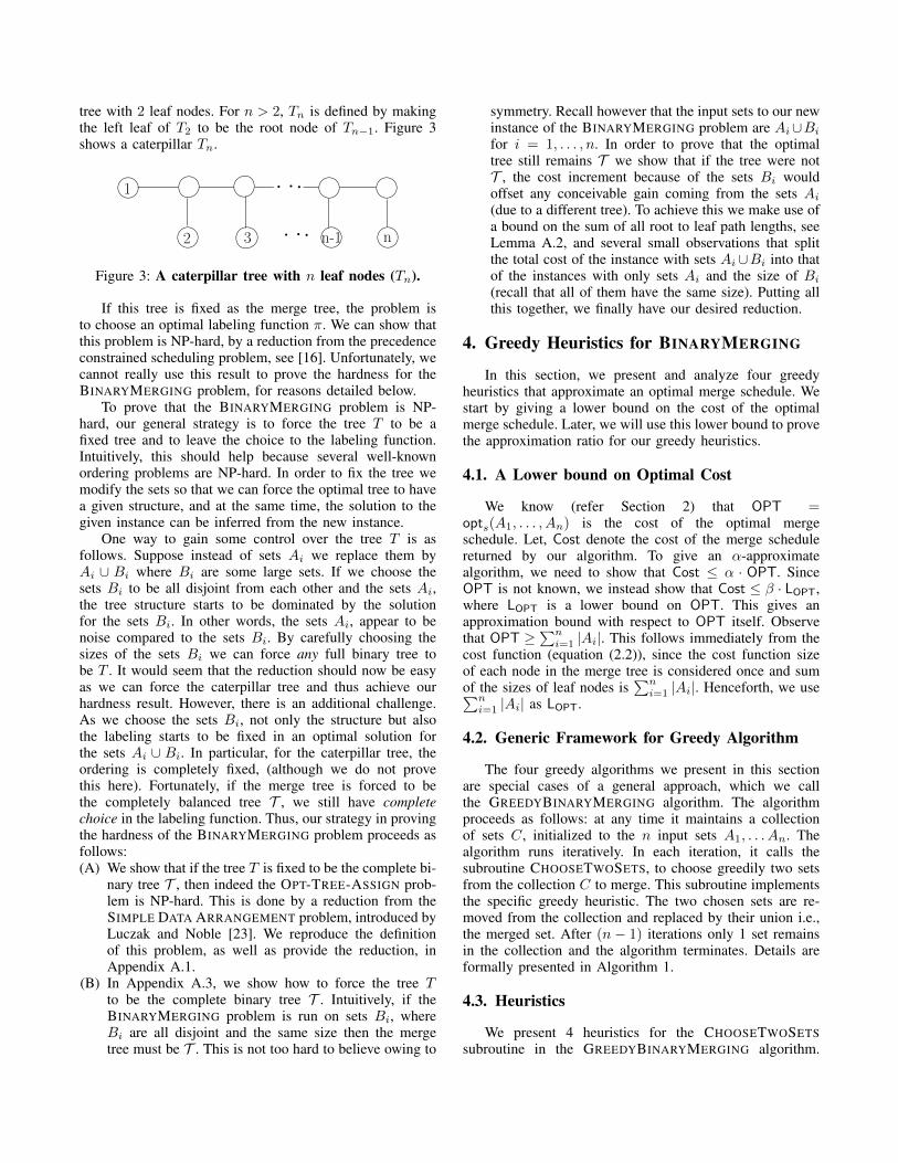
tree with 2 leaf nodes. For n > 2, Tn is defined by makingthe left leaf of T

2

to be the root node of Tn�1

. Figure 3shows a caterpillar Tn.

1

2 3 n-1 n

Figure 3: A caterpillar tree with n leaf nodes (Tn).

If this tree is fixed as the merge tree, the problem isto choose an optimal labeling function ⇡. We can show thatthis problem is NP-hard, by a reduction from the precedenceconstrained scheduling problem, see [16]. Unfortunately, wecannot really use this result to prove the hardness for theBINARYMERGING problem, for reasons detailed below.

To prove that the BINARYMERGING problem is NP-hard, our general strategy is to force the tree T to be afixed tree and to leave the choice to the labeling function.Intuitively, this should help because several well-knownordering problems are NP-hard. In order to fix the tree wemodify the sets so that we can force the optimal tree to havea given structure, and at the same time, the solution to thegiven instance can be inferred from the new instance.

One way to gain some control over the tree T is asfollows. Suppose instead of sets Ai we replace them byAi [ Bi where Bi are some large sets. If we choose thesets Bi to be all disjoint from each other and the sets Ai,the tree structure starts to be dominated by the solutionfor the sets Bi. In other words, the sets Ai, appear to benoise compared to the sets Bi. By carefully choosing thesizes of the sets Bi we can force any full binary tree tobe T . It would seem that the reduction should now be easyas we can force the caterpillar tree and thus achieve ourhardness result. However, there is an additional challenge.As we choose the sets Bi, not only the structure but alsothe labeling starts to be fixed in an optimal solution forthe sets Ai [ Bi. In particular, for the caterpillar tree, theordering is completely fixed, (although we do not provethis here). Fortunately, if the merge tree is forced to bethe completely balanced tree T , we still have completechoice in the labeling function. Thus, our strategy in provingthe hardness of the BINARYMERGING problem proceeds asfollows:(A) We show that if the tree T is fixed to be the complete bi-

nary tree T , then indeed the OPT-TREE-ASSIGN prob-lem is NP-hard. This is done by a reduction from theSIMPLE DATA ARRANGEMENT problem, introduced byLuczak and Noble [23]. We reproduce the definitionof this problem, as well as provide the reduction, inAppendix A.1.

(B) In Appendix A.3, we show how to force the tree Tto be the complete binary tree T . Intuitively, if theBINARYMERGING problem is run on sets Bi, whereBi are all disjoint and the same size then the mergetree must be T . This is not too hard to believe owing to

symmetry. Recall however that the input sets to our newinstance of the BINARYMERGING problem are Ai[Bi

for i = 1, . . . , n. In order to prove that the optimaltree still remains T we show that if the tree were notT , the cost increment because of the sets Bi wouldoffset any conceivable gain coming from the sets Ai

(due to a different tree). To achieve this we make use ofa bound on the sum of all root to leaf path lengths, seeLemma A.2, and several small observations that splitthe total cost of the instance with sets Ai[Bi into thatof the instances with only sets Ai and the size of Bi

(recall that all of them have the same size). Putting allthis together, we finally have our desired reduction.

4. Greedy Heuristics for BINARYMERGING

In this section, we present and analyze four greedyheuristics that approximate an optimal merge schedule. Westart by giving a lower bound on the cost of the optimalmerge schedule. Later, we will use this lower bound to provethe approximation ratio for our greedy heuristics.

4.1. A Lower bound on Optimal Cost

We know (refer Section 2) that OPT =

opts(A1

, . . . , An) is the cost of the optimal mergeschedule. Let, Cost denote the cost of the merge schedulereturned by our algorithm. To give an ↵-approximatealgorithm, we need to show that Cost ↵ · OPT. SinceOPT is not known, we instead show that Cost � · LOPT,where LOPT is a lower bound on OPT. This gives anapproximation bound with respect to OPT itself. Observethat OPT �

Pni=1

|Ai|. This follows immediately from thecost function (equation (2.2)), since the cost function sizeof each node in the merge tree is considered once and sumof the sizes of leaf nodes is

Pni=1

|Ai|. Henceforth, we usePni=1

|Ai| as LOPT.

4.2. Generic Framework for Greedy Algorithm

The four greedy algorithms we present in this sectionare special cases of a general approach, which we callthe GREEDYBINARYMERGING algorithm. The algorithmproceeds as follows: at any time it maintains a collectionof sets C, initialized to the n input sets A

1

, . . . An. Thealgorithm runs iteratively. In each iteration, it calls thesubroutine CHOOSETWOSETS, to choose greedily two setsfrom the collection C to merge. This subroutine implementsthe specific greedy heuristic. The two chosen sets are re-moved from the collection and replaced by their union i.e.,the merged set. After (n� 1) iterations only 1 set remainsin the collection and the algorithm terminates. Details areformally presented in Algorithm 1.

4.3. Heuristics

We present 4 heuristics for the CHOOSETWOSETSsubroutine in the GREEDYBINARYMERGING algorithm.

1 Algorithm GREEDYBINARYMERGING(A1

, . . . An)2 C {A

1

, . . . , An};3 for i = 1, . . . , n� 1 do4 S

1

, S2

CHOOSETWOSETS(C);5 C C \ {S

1

, S2

};6 C C [ {S

1

[ S2

};7 end

Algorithm 1: Generic greedy algorithm.

We show that three of these heuristics are O(log n)-approximations. To explain the algorithms we will use thefollowing working example:

Working Example. We are given as input 5 sets: A1

=

{1, 2, 3, 5}, A2

= {1, 2, 3, 4}, A3

= {3, 4, 5}, A4

=

{6, 7, 8}, A5

= {7, 8, 9}. The goal is to merge them into asingle set such that the merge cost as defined in Section 2is minimized.

4.3.1. BALANCETREE (BT) Heuristic. Assume for sim-plicity that n is a power of 2. One natural heuristic for theproblem is to merge in a way such that the underlying mergetree is a complete binary tree. This can be easily done asfollows: the input sets form the leaf nodes or level 1 nodes.The n leaf nodes are arbitrarily divided into n/2 pairs. Thepaired sets are merged to get the level 2 nodes. In general,the level i nodes are arbitrarily divided into n/2i pairs. Eachpair is merged i.e., the corresponding sets are merged to getn/2i nodes in the i+1

th level. This builds a complete binarytree of height log n.

However, when n is not a power of 2, to create a mergetree of height dlog ne involves a little more technicality. Todo this, annotate each set with its level number l, and letminL be the minimum level number across all sets at anypoint of time. Initially, all the sets are marked with l = 1.In each iteration, we choose two sets whose level numberis minL, merge these sets, and assign the new mergedset the level (minL + 1). If only 1 set exists with levelnumber equal to minL, we increment its l by 1 and retrythe process. Figure 4 shows the merge schedule obtainedusing this heuristic on our working example.

Lemma 4.1. Consider an instance A1

, . . . , An of the BI-NARYMERGING problem. BALANCETREE heuristic, givesa (dlog ne+ 1)-approximation.

Proof. Let T be the merge tree constructed. By our level-based construction, height(T ) = dlog ne. Let Cl denote thecollection of sets at level l. Now observe that each set in Cl

is either the union of some initial sets, or is an initial set byitself. Also, each initial set participates in the constructionof atmost 1 set in Cl. This implies that:

X

S2Cl

|S| nX

i=1

|Ai| = LOPT OPT

1 2

3

4

{1,2,3,4,5} {3,4,5,6,7,8}

{1,2,3,4,5,6,7,8} {7,8,9}

{1,2,3,4,5,6,7,8,9}

A1 A2 A3 A4

A5

{1,2,3,5} {1,2,3,4} {3,4,5} {6,7,8}

Figure 4: Merge schedule using BALANCETREE heuris-tic. The label inside the leaf nodes denotes the corre-sponding set. The label inside internal nodes denotethe iteration in which the merge happened. The setscorresponding to each node is shown outside the node.Cost of the merge = 45.

Therefore,

Cost =

dlogne+1X

l=1

X

S2Cl

|S| (dlog ne+ 1) · OPT

⌅

Lemma 4.2. The approximation bound proved forBALANCETREE in Lemma 4.1 heuristic is tight.

Proof. We show an example where the merge cost obtainedby using BALANCETREE heuristic is ⌦(log n) ·OPT. Con-sider n initial sets where n is a power of 2. The setsare A

1

= {1}, A2

= {1}, . . . , An�1

= {1}, An =

{1, 2, 3, . . . n}, i.e., we have (n � 1) identical sets whichcontain just the element 1, and one set which has n elements.An optimal merge schedule is the left-to-right merge, i.e.,it starts by merging A

1

and A2

to get the set A1

[ A2

,then merges A

1

[ A2

with A3

to get A1

[ A2

[ A3

andso on. The cost of this merge is (4n � 3). However theBALANCETREE heuristic creates a complete binary tree ofheight log n, and the large n size set {1, 2, . . . , n} appears inevery level. Thus the cost will be atleast n ·(log n+1). Thislower bounds the approximation ratio of BALANCETREEheuristic to ⌦(log n). ⌅

4.3.2. SMALLESTINPUT (SI) Heuristic. This heuristic se-lects in each iteration, those two sets in the collection thathave the smallest cardinality. The intuitive reason behindthis approach is to defer till later the larger sets and thus,reduce the recurring effect on cost. Figure 5 shows themerge tree we obtain when we run the greedy algorithmwith SMALLESTINPUT heuristic on our working example.

4.3.3. SMALLESTOUTPUT (SO) Heuristic. In each itera-tion, this heuristic chooses those two sets in the collectionwhose union has the least cardinality. The intuition behindthis approach is similar to SI. In particular, when the setsA

1

, . . . , An are all disjoint, these two heuristics lead to the

1 2

3

4

{3,4,5,6,7,8} {1,2,3,4,7,8,9}

{1,2,3,4,5,6,7,8}

{7,8,9}

{1,2,3,4,5,6,7,8,9}

A3 A4 A5 A2

A1

{3,4,5} {6,7,8} {1,2,3,4}

{1,2,3,5}

Figure 5: Merge schedule using SMALLESTINPUT heuris-tic. Initially the smallest sets are A

3

, A4

, A5

. The algo-rithm arbitrarily choses A

3

and A4

to merge, creatingnode 1 with corresponding set {3, 4, 5, 6, 7, 8}. Next thealgorithm proceeds with merging A

1

and A2

as they arethe current smallest sets in collection, and so on. Costof the merge = 47.

1

2

3

4

{6,7,8,9}

{1,2,3,4,5}

{1,2,3,4,5}

{3,4,5}

{1,2,3,4,5,6,7,8,9}

A4 A5

A1 A2

A3

{6,7,8} {7,8,9}

{1,2,3,5} {1,2,3,4}

Figure 6: Merge schedule using SMALLESTOUTPUTheuristic. Initially the smallest output set is obtained bymerging sets A

4

, A5

. In first iteration A4

, A5

is mergedto get the new set {6, 7, 8, 9}. Next the algorithm choosesA

1

, A2

to merge as they create the smallest output ofsize 4, and so on. Cost of the merge = 40.

same algorithm. Figure 6 depicts the merge tree we obtainwhen executed on our working example.

Lemma 4.3. Given n disjoint sets A1

, . . . , An, the BI-NARYMERGING problem can be solved optimally usingSMALLESTINPUT (or SMALLESTOUTPUT) heuristics.

Proof. As we remarked in Section 2 that for this specialcase, the BINARYMERGING problem reduces to the Huff-man coding problem, and as is well known, the above greedyheuristic is indeed the optimal greedy algorithm for prefixfree coding [20]. ⌅Lemma 4.4. Consider an instance A

1

, . . . , An of the BI-NARYMERGING problem. Both the SMALLESTINPUT andSMALLESTOUTPUT heuristics, give O(log n) approximatesolutions.

Proof. Let Aj1

, , . . . , Ajn�j , be the sets left after the jth

iteration of the algorithm. Now observe that each Aji is

either the union of some initial sets, or is an initial set itself.Further each initial set contributes to exactly 1 of the Aj

i ’s.This implies that:

n�jX

i=1

���Aji

��� nX

i=1

|Ai| = LOPT OPT

Without loss of generality, let us assume that after j itera-tions, Aj

1

and Aj2

are the two smallest cardinality sets left.We can show that (see Lemma B.1):

���Aj1

[Aj2

��� ���Aj

1

���+���Aj

2

��� 2

n� j

n�jX

i=1

���Aji

���

If the greedy algorithm uses the SMALLESTINPUT heuristic,then in the (j + 1)

th iteration, sets Aj1

, Aj2

will be chosento be merged. In case of the SMALLESTOUTPUT heuristic,we choose the two sets that give the smallest output set. LetCj+1

be the output set created in the (j + 1)

th iteration.Combining the above we can say that:

Cj+1

���Aj

1

[Aj2

��� 2

n� j· OPT

Thus, for either of the greedy strategies, SMALLESTINPUTand SMALLESTOUTPUT, the total cost is:

Cost nX

i=1

|Ai|+n�1X

j=1

|Cj | OPT+

n�1X

j=1

2

n� j + 1

· OPT

(2Hn + 1) · OPT [Hn is the nth harmonic number]

⌅

Lemma 4.5. The greedy analysis is tight with respect to thelower bound for optimal (LOPT).

Proof. We show an example where the ratio of thecost of merge obtained by using SMALLESTINPUT orSMALLESTOUTPUT heuristic and LOPT is log n. Considern initial sets where n is a power of 2. The sets areA

1

= {1}, . . . , Ai = {i}, . . . , An = {n}, i.e., each setis of size 1 and they are disjoint. The lower bound we usedfor the greedy analysis is LOPT =

Pni=1

|Ai| = n. Boththe heuristics, SMALLESTINPUT and SMALLESTOUTPUT,creates a complete binary tree of height log n. Since theinitial sets are disjoint, the collection of sets in each levelis also disjoint and the total size of the sets in each level isn. Thus the total merge cost is n · log n = log n · LOPT. ⌅

Remark. Lemma 4.5 gives a lower bound with respectto LOPT, and not OPT. It suggests that the approximationratio cannot be improved unless the lower bound (LOPT) isrefined. Finding a bad example with respect to OPT is anopen problem.

4.3.4. LARGESTMATCH Heuristic. In each iteration, thisapproach chooses those two sets that have largest intersec-tion [6]. However, the worst case performance bound forthis heuristic can be arbitrarily bad. It can be shown that theapproximation bound for this algorithm is ⌦(n). Consider acollection of n sets, where set Ai = {1, 2, . . . , 2i�1}, for alli 2 [n]. The optimal way of merging is left-to-right merge.The cost of this merge is 1+2·(2+4+. . . 2n�1

) = 2

n+1�3.However, the LARGESTMATCH heuristic will always choose{1, 2, . . . , 2n�1} as one of the sets in each iteration as it haslargest intersection with any other set. Thus the cost will be2

n�1 ·(n�1). This shows a gap of ⌦(n) between the optimalcost and LARGESTMATCH heuristic.

4.4. An f -approximation for BINARYMERGING

For each element x in U , let fx denote the number ofinitial sets to which x belongs, i.e., the fx is frequencyof x in the initial sets. Let f = maxx2U fx denote themaximum frequency across all elements. We present anf -approximation algorithm for BINARYMERGING. If f issmall, i.e., the elements do not belong to a large number ofsets, then this algorithm gives stronger approximation boundthan the preceding algorithms. The algorithm is shown inAlgorithm 2 and proceeds as follows: we create a dummyset A0

i corresponding to each initial set Ai. These dummysets are obtained by replacing each element in a set by atuple, which consists of the element and the set number.Note that dummy sets created in this manner are disjoint. Werun the GREEDYBINARYMERGING on the sets A0

1

, . . . A0n

using SMALLESTINPUT (or SMALLESTOUTPUT) heuristicto obtain the tree T 0 and leaf assignment function ⇡0. Finally,we use the same T 0, and ⇡0 to merge the initial sets. Theintuition behind the algorithm is as follows: once the sets aredisjoint our algorithms perform optimally and the resultanttree can be used as a guideline for merging.

1 Algorithm FREQBINARYMERGING(A1

, . . . An)2 Corresponding to each set Ai create a new set

A0i, where A0

i = {(x, i) : x 2 Ai};3 Run GREEDYBINARYMERGING on

A01

, A02

, . . . , A0n with SMALLESTINPUT heuristic;

4 Let T 0 be the tree and ⇡0 be the leaf assignment;5 Merge A

1

, . . . An using T 0, and ⇡0

Algorithm 2: f -approx for BINARYMERGING.

Lemma 4.6. Algorithm 2 is an f -approximation algorithmfor BINARYMERGING.

Proof. Let OPT0 be the optimal merge cost for the in-stance A0

1

, . . . A0n. Let Cost0 be the cost of the greedy

solution. The sets A01

, . . . A0n are disjoint by construction. By

Lemma 4.3, the SMALLESTINPUT (or SMALLESTOUTPUT)heuristic gives the optimal solution in this case. This impliesOPT0

= Cost0. Let ⌫ be any node in T 0. Le A0⌫ be its

label for the instance A01

, . . . A0n and A⌫ be its label for

the instance A1

, . . . An. A⌫ is union of some initial sets,and A0

⌫ is the union of corresponding modified initial setswhich are disjoint. It follows that |A⌫ | |A0

⌫ |. Summingwe get, Cost Cost0 = OPT0.

For the instance A1

, . . . An, let TOPT be the optimaltree, and ⇡OPT be the leaf assignment . Now if A0

1

, . . . A0n

was merged using TOPT and ⇡OPT , then the cost of themerge will be at most f ·OPT. This follows from the fact thatsize of each node in the new tree is atmost f times the sizeof the corresponding node in the optimal tree, as each setcan contain atmost f renamed copies of the same element.Since TOPT and ⇡OPT are not optimal for A0

1

, . . . A0n the

resulting merge cost is atleast OPT0 i.e., OPT0 f ·OPT.Combining we get, Cost f · OPT. ⌅

5. Simulation ResultsIn this section, we evaluate our greedy strategies from

Section 4 in practice. Our experiments answer the followingquestions:• Which compaction strategy should be used in practice,

given real-life workloads?• How close is a given compaction strategy to optimal?• How effective is the cost function in modeling running

time for compaction?

5.1. Setup

Dataset. We generated the dataset from an industrybenchmark called YCSB (Yahoo Cloud Servicing Bench-mark) [17]. YCSB generates CRUD (create, read, update,delete) operations for benchmarking a key-value store emu-lating a real-life workload. There are parameters importantin YCSB which we explain next. YCSB works in twodistinct phases: 1) load: inserts keys to an empty database.The recordcount parameter controls the number of insertedkeys. 2) run: generates CRUD operations on the loadeddatabase. The operationcount parameter controls the numberof operations.

Our experiments only consider insert and update oper-ations in order to load memtables (and thus, sstables). Wedo not consider deletes or reads. Deletes are handled byappending a tombstone to the memtable. When compactionencounters a tombstone, it removes the associated key fromthe database. This handling is very similar to normal up-date operations and thus, we chose to ignore deletes forsimplicity. Reads do not modify sstables and thus, are notgenerated.

In YCSB, update operations access keys using one ofthe three realistic distributions: 1) Uniform: All the insertedkeys are uniformly accessed, 2) Zipfian: Some keys are morepopular than others (power-law), and 3) Latest: Recentlyinserted keys are more popular (power-law).

Cluster. We ran our experiments in the Illinois CloudComputing Testbed [5] which is part of the Open Cirrusproject [14]. We used a single machine with 2 quad coreCPUs, 16 GB of physical memory and 2 TB of disk capacity.The operating system running is CentOS 5.9.

(a) (b)

Figure 7: Cost and time for compacting sstables generated by varying update percentage with latest distribution.

Simulator. Our simulator works in two distinct phases. Inthe first phase, we create sstables. YCSB’s load and runphases generates operations which are first inserted into afixed size (number of keys) memtable. When the memtableis full, it is flushed as an sstable and a new empty memtableis created for subsequent writes. As a memtable may containduplicate keys, sstables may be smaller and vary in size.

In the second phase, we merge the generated sstablesusing some of the compaction strategies proposed in Sec-tion 4. By default, the number of sstables we merge in aniteration, k is set to 2. We measure the cost and time atthe end of compaction for comparison. The cost representscostactual defined in Section 2. The running time measuresboth the strategy overhead and the actual merge time.

We evaluate the following 5 compaction strategies:1) SMALLESTINPUT (SI): In this strategy, we choose the

k smallest cardinality sstables at each iteration (Sec-tion 4.3.2). We implement this via a priority queue to findthe smallest cardinality sstables. This implementationworks in O(log n) time per iteration.

2) SMALLESTOUTPUT (SO): In this strategy, we choosethe k sstables whose union has the smallest cardinality(Section 4.3.3). Calculating the cardinality of an outputsstable without actually merging the input sstables istricky. We estimate cardinality of the output sstable usingHyperloglog [18] (HLL). We compute the HLL estimatefor all

�nk

�combinations of sstables in the first iteration.

At the end of the iteration, k sstables are removed anda new sstable is added. In the next iteration, we haveto compute the estimates for

�n�k+1

k

�combinations. We

can reduce this number by making the following twoobservations: 1) some of the estimates from the lastiteration (involving sstables not removed) can be reusedand 2) compute estimate for only those combinationswhich involve the new sstable. Thus, the total number ofcombinations for which we need to estimate cardinalityis

�n�kk�1

�. The per-iteration overhead for this strategy is

high.3) BALANCETREE with SMALLESTINPUT at each level

(BT (I)): This strategy merges sstables in a singlelevel together (Section 4.3.1). Since all sstables at a

single level can be simultaneously merged, we usethreads to parallelly initiate multiple merge opera-tions. BALANCETREE does not specify a order forchoosing sstables to merge in a single level. We useSMALLESTINPUT strategy and pick sstables in the in-creasing order of their cardinality.

4) BALANCETREE with SMALLESTOUTPUT at each level(BT (O)): This is similar to BT (I) strategy except weuse SMALLESTOUTPUT for finding sstables to mergetogether at each level. Even though, the SO strategy hasa large per-iteration strategy overhead, the overhead forthis strategy is amortized over multiple iterations thathappen in a single level.

5) RANDOM: As a strawman to compare against, we imple-mented a random strategy that picks random k sstables tomerge (at each iteration). This represents the case whenthere is no compaction strategy. It will thus provide abaseline to compare with.

5.2. Strategy Comparison

We compare the compaction heuristics from Section 4using real-life (YCSB) workloads. We fixed the opera-tioncount at 100K, recordcount at 1000 and memtable sizeat 1000. We varied the workload along a spectrum frominsert heavy (insert proportion 100% and update proportion0%) to update heavy (update proportion 100% and insertproportion 0%). We ran experiments with all 3 key accessdistributions in YCSB.

With 0% updates, the workload only comprises of newkeys. With 100% updates, all the keys inserted in the loadphase will be repeatedly updated implying a larger intersec-tion among sstables. When keys are generated with a power-law distribution (zipfian or latest) the intersections increaseas there will be a few popular keys updated frequently. Wepresent result for latest distribution only. The observationsare similar for zipfian and uniform and thus, excluded.

Figures 7 plots the average and the standard deviationfor cost and time for latest distribution from 3 independentruns of the experiment. We observe that SI and BT (I)have a compaction cost that is marginally lower than BT (O)

(for latest distribution) and SO. Compaction using BT (I)finishes faster compared to SI because of its parallel im-plementation. RANDOM is the worst strategy. Thus, BT (I)is the best choice to implement in practice. As updatesincrease, the cost of compaction decreases for all strate-gies. With a fixed operationcount, larger intersection amongsstables implies fewer unique keys, which in turn impliesfewer disk writes.

RANDOM is much worse than our heuristics at smallupdate percentage. This can be attributed to the balancednature of the merge trees. Since sstables are flushed to diskwhen the memtable reaches a size threshold, the sizes of theactual sstable have a small deviation. Merging two sstables(S

1

and S2

) of similar size with small intersection (smallupdate percentage) creates another sstable (S

3

) of roughlydouble the size at the next level. Both SI and SO chooseS3

for merge only after all the sstables in the previous levelhave been merged. Thus, their merged trees are balancedand their costs are similar. On the contrary, RANDOM mightselect S

3

earlier and thus, have a higher cost.As the intersections among sstables increase (with in-

creasing update percentage), the size of sstables in the nextlevel (after a merge) is close to the previous level. At thispoint, it is immaterial which sstables are chosen at eachiteration. Irrespective of the merge tree, the cost of a mergeis constant 2. Thus, RANDOM performs as well as the otherstrategies when the update percentage is high.

The cost of SO and BT (O) is sensitive to the error incardinality estimation. The generated merge schedule differsfrom the one generated by the naive sstable merging schemewhich accurately identifies the smallest union. This resultsin slightly higher overall cost. The running time of SOincreases linearly as updates increase because cardinality es-timation overhead increases as intersections among sstablesincrease.

5.3. Comparison with Optimal

In this experiment, we wish to evaluate how closeBT (I), our best strategy, is to optimal. Extensively search-ing all permutations of merge schedules for finding theoptimal cost for large number and size of sstable is pro-hibitive and exponentially expensive. Instead, we calculatethe sum of sstable sizes, our known lower bound for optimalcost from Section 4.1. We vary the memtable size from10 to 10K and fix the number of sstables to 100. Therecordcount for load stage is 1000 and update insert ratiois set to 60:40. The number of operations (operationcount)for YCSB is calculated as: memtable size(10 to 10K) ⇥number of sstables (100)� recordcount (1000). We ran ex-periments for all three key access distributions.

Figure 8 compares the cost of merge using BT (I) withthe lower-bounded optimal cost, averaged over 3 indepen-dent runs of the experiment. Both x and y-axis use logscale. As the maximal memtable size (before flush) increases

2. If sstable size is s, number of sstables to merge in an iteration is 2and the number of sstables is n, then costactual would be 3 · (n� 1) · s.

Figure 8: Comparing cost of BT (I) to optimal which islower bounded by sum of sizes of all sstables. Both xand y-axis are in log scale.

exponentially, both the curves show a linear increase in logscale with similar slope. Thus, in real life workloads, thecost of our strategy is within a constant factor of the lowerbound of the optimal cost. This is a better performance thanthe analyzed worst case O(log n) bound (Lemma 4.5).

5.4. Cost Function Effectiveness

In Section 2 we defined costactual to model amount ofdata to be read from and written to disk. This cost alsodetermines the running time for compaction. The goal ofthis experiment is to validate how the defined cost functionaffects the compaction time. In this experiment, we comparethe cost and time for SI . We chose this strategy because ofits low overhead and single-threaded implementation. Weran our experiments with the same settings as described inSection 5.2 and Section 5.3. Cost and time values are cal-culated by averaging the observed values of 3 independentruns of the experiment.

Figure 9 plots the cost on x-axis and time on y-axis.As we increase update proportion ((Figure 9b) and opera-tioncount (Figure 9a), we see an almost linear increase fortime as cost increases for all 3 distributions. This validatesthe cost function in our problem formulation, as by mini-mizing it, we will reduce the running time as well.

6. Conclusion

In this work, we formulated compaction in key valuestores as an optimization problem. We proved it to be NP-hard. We proposed 3 heuristics and showed them to beO(log n) approximations. We implemented and evaluatedthe proposed heuristics using real-life workloads. We foundthat a balanced tree based approach BT (I) provides the besttradeoff in terms of cost and time.

Many interesting theoretical questions still remain.The O(log n) approximation bound shown for the

(a) Increasing update percentage (b) Increasing operationcount

Figure 9: Effect of cost function on completion time for compaction. SI strategy used. Update Percentage and datasizevaried for the plots respectively.

SMALLESTINPUT and SMALLESTOUTPUT heuristic seemsquite pessimistic. Under real-life workloads, the algorithmsperform far better than O(log n). We do not know of any badexample for these two heuristics showing that the O(log n)bound is tight. This naturally motivates the question, if theright approximation bound is infact O(1). Finally, it will beinteresting to study the hardness of approximation for theBINARYMERGING problem.

Acknowledgement. We thank Chandra Chekuri for helpfuldiscussions and insightful ideas regarding proofs and plots.

References

[1] Cassandra. http://cassandra.apache.org/. visited on 2014-04-29.

[2] CouchDB. http://couchdb.apache.org. visited on 2014-04-29.

[3] Date Tiered Compaction. https://issues.apache.org/jira/browse/CASSANDRA-6602. visited on 2014-11-20.

[4] HBase. https://hbase.apache.org. visited on 2014-04-29.

[5] Illinois Cloud Computing Testbed. http://cloud.cs.illinois.edu/. visitedon 2014-11-20.

[6] Improving compaction in Cassandra with cardinality estima-tion. http://www.datastax.com/dev/blog/improving-compaction-in-cassandra-with-cardinality-estimation. visited on 2014-12-09.

[7] LevelDB. http://google-opensource.blogspot.com/2011/07/leveldb-fast-persistent-key-value-store.html. visited on 2014-11-24.

[8] LevelDB in Riak. http://docs.basho.com/riak/latest/ops/advanced/backends/leveldb/. visited on 2014-11-24.

[9] Leveled Compaction in Cassandra. http://www.datastax.com/dev/blog/leveled-compaction-in-apache-cassandra. visited on 2014-11-24.

[10] Riak. http://basho.com/riak/. visited on 2014-04-29.

[11] RocksDB. http://rocksdb.org/. visited on 2014-11-20.

[12] Size Tiered Compaction. http://shrikantbang.wordpress.com/2014/04/22/size-tiered-compaction-strategy-in-apache-cassandra/. visited on2014-11-20.

[13] G. S. Brodal and R. Fagerberg. Lower bounds for external memorydictionaries. In Proceedings of the Fourteenth Annual ACM-SIAMSymposium on Discrete Algorithms, SODA ’03, pages 546–554,Philadelphia, PA, USA, 2003. Society for Industrial and AppliedMathematics.

[14] R. Campbell, I. Gupta, M. Heath, S. Y. Ko, M. Kozuch, M. Kunze,T. Kwan, K. Lai, H. Y. Lee, M. Lyons, D. Milojicic, D. O’Hallaron,and Y. C. Soh. Open Cirrus Cloud Computing Testbed: FederatedData Centers for Open Source Systems and Services Research. InProceedings of the 2009 Conference on Hot Topics in Cloud Comput-ing, HotCloud’09, Berkeley, CA, USA, 2009. USENIX Association.

[15] F. Chang, J. Dean, S. Ghemawat, W. C. Hsieh, D. A. Wallach,M. Burrows, T. Chandra, A. Fikes, and R. E. Gruber. Bigtable:A distributed storage system for structured data. In Proceedingsof the 7th USENIX Symposium on Operating Systems Design andImplementation - Volume 7, OSDI ’06, pages 15–15, Berkeley, CA,USA, 2006. USENIX Association.

[16] C. Chekuri and R. Motwani. Precedence constrained scheduling tominimize sum of weighted completion times on a single machine.Discrete Applied Mathematics, 98(12):29 – 38, 1999.

[17] B. F. Cooper, A. Silberstein, E. Tam, R. Ramakrishnan, and R. Sears.Benchmarking Cloud Serving Systems with YCSB. In Proceedingsof the 1st ACM Symposium on Cloud Computing, SoCC ’10, pages143–154, New York, NY, USA, 2010. ACM.

[18] P. Flajolet, E. Fusy, O. Gandouet, and F. Meunier. Hyperloglog:The analysis of a near-optimal cardinality estimation algorithm. InIN AOFA 07: Proceedings of the 2007 International Conference onAnalysis of Algorithms, 2007.

[19] M. Frigo, C. E. Leiserson, H. Prokop, and S. Ramachandran. Cache-oblivious algorithms. ACM Transactions on Algorithms (TALG),8(1):4:1–4:22, Jan. 2012.

[20] D. Huffman. A method for the construction of minimum-redundancycodes. Proceedings of the IRE, 40(9):1098–1101, Sept 1952.

[21] A. Lakshman and P. Malik. Cassandra: A decentralized structuredstorage system. ACM SIGOPS Operating Systems Review, 44(2):35–40, Apr. 2010.

[22] L. Lovsz. Submodular functions and convexity. In A. Bachem,B. Korte, and M. Grtschel, editors, Mathematical Programming TheState of the Art, pages 235–257. Springer Berlin Heidelberg, 1983.

[23] M. J. Luczak and S. Noble. Optimal arrangement of data in a treedictionary. Discrete Applied Mathematics, 113:243–253, 2001.

[24] C. Mathieu, C. Staelin, and N. E. Young. K-slot sstable stackcompaction. CoRR, abs/1407.3008, 2014.

[25] H. T. Vo, S. Wang, D. Agrawal, G. Chen, and B. C. Ooi. Logbase:A scalable log-structured database system in the cloud. Proceedingsof the VLDB Endowment, 5(10):1004–1015, June 2012.

Appendix A.We now formally prove that BINARYMERGING is NP-hard.

A.1. The SIMPLE DATA ARRANGEMENT problem

The following problem, known as the SIMPLE DATAARRANGEMENT problem is discussed in the paper ofLuczak and Noble [23]. The problem is defined as follows:Instance: Given graph G = (V,E) and a nonnegativeinteger B given in binary.Question: Is there an injective mapping f from V to theleaves of a complete d-ary tree T , of height dlogd |V |e, suchthat

P{i,j}2E dT (f(i), f(j)) B?

Luczak and Noble show in [23], that the above prob-lem is NP-hard for any d � 2. We notice that in theabove, we may assume that |V | is an exact power of d,i.e., |V | = dlogd|V |. The SIMPLE DATA ARRANGEMENTproblem reduces to such special cases, and so this variantis also NP-hard.

A.2. A problem related to BINARYMERGING

We consider the following problem which is related tothe BINARYMERGING problem. In this problem we aregiven n sets A

1

, . . . , An, and a full binary tree T withn leaves, and the problem is to find a labeling func-tion ⇡ which assigns the sets to the leaves such thatcost(T,⇡, A

1

, . . . , An) is minimized. Notice that the onlydifference with the BINARYMERGING problem is that herewe are fixing the tree T while the BINARYMERGING prob-lem seems somewhat harder. Let OPT-TREE-ASSIGN denotethis problem, and for an instance with sets A

1

, . . . , An andthe full binary tree T with n leaves, let opta(T,A1

, . . . , An)

denote the value of optimal solution. Let n = 2

h be a powerof 2, and let T be a perfectly balanced tree with n leaves,and height h = log n. We first show the following

Lemma A.1. The OPT-TREE-ASSIGN problem is NP-hard,for instances where the number of sets n is a power of two,and the tree input T is the balanced binary tree T .

Proof. Consider a given instance of the SIMPLE DATA AR-RANGEMENT problem: we have a graph G = (V,E), where|V | = n = 2

h for some integer h, and an integer B inbinary. We define n sets, Ai, one for each vertex i, wherewe assume that the vertices have been labeled as 1, . . . , n.Suppose that e

1

, . . . , ek are the edges incident to a vertex i.Then we define Ai = {e

1

, . . . , ek}. We consider the instanceof the OPT-TREE-ASSIGN problem given by the sets Ai for1 i n and the complete binary tree T with n = 2

h leafnodes. Suppose ⇡ : [n] ! [n] is any labeling function, thatassigns the set Ai to the leaf numbered ⇡(i). Clearly, thesize of this instance is only polynomially larger than that ofthe given instance of the SIMPLE DATA ARRANGEMENTproblem, which we assume has size at least |V | + |E|.Now we use the reformulation of the cost function for theOPT-TREE-ASSIGN problem as given in Section 2. Supposee = (i, j) is an edge of G. Clearly e occurs in exactly twoof the sets Ai, Aj . Further the cost T (e) can be seen to be

exactly, log n +

1

2

dT (⇡(i),⇡(j)). Therefore, the total costfor the OPT-TREE-ASSIGN using the labeling ⇡ is,

cost(T ,⇡, A1

, . . . , An) = |E| log n+1

2

X

e=(i,j)

dT (⇡(i),⇡(j)).

Therefore, we have that,

min

labelings ⇡

X

e=(i,j)

dT (⇡(i),⇡(j)) = 2opta(T , A1

, . . . , An)

�2 |E| log n

Notice that min

labelings ⇡

Pe=(i,j)

dT (⇡(i),⇡(j)) is precisely the

cost of the best injective mapping for the SIMPLE DATAARRANGEMENT problem. Therefore, a polynomial timealgorithm for the OPT-TREE-ASSIGN problem would helpus evaluate this number and then we can decide if it is lessthan B. Our reduction is complete. ⌅

A.3. Forcing a complete binary tree

Let T be a binary tree with n = 2

h leaves for someinteger h. Let r be the root node of T . Let ⌘(T ) be the sumof the root to leaf node distances for all the leaf nodes, i.e.,

⌘(T ) =X

⌫ leaf node of T

dT (r, ⌫),

Lemma A.2. For any binary tree T with n leaf nodes, wehave that ⌘(T ) � n log n with equality only for the perfectbinary tree; here n = 2

h for some integer h.

Proof. This holds if T has only 1 leaf node. We may assumethat T is a full binary tree, otherwise the value of ⌘(T ) canbe decreased. Any full tree must have at least 2 leaf nodesand we can easily verify that the given result holds here.We use induction to prove the result for n > 2. Supposethat the root r has two full trees T

1

and T2

as childrenwith n

1

, n2

leaf nodes respectively. We have, n = n1

+ n2

and, ⌘(T ) = ⌘(T1

) + ⌘(T2

) + n1

+ n2

. As n1

, n2

< n, weuse the induction assumption to get that ⌘(T

1

) � n1

log n1

and similarly for T2

. Now using the strict convexity of thefunction f(x) = x log x for x > 0 we immediately get that⌘(T ) � n log n. For equality, both T

1

and T2

must achieveequality and moreover they must have the same numberof leaf nodes, i.e., n

1

= n2

= 2

k for some k. Moreover,they must both be complete trees. This means T is also acomplete binary tree with n = 2

k+1 leaf nodes. ⌅Given n sets A

1

, . . . , An with m elements, let T be anyfull binary tree on n leaves, and ⇡ be the leaf assignmentfunction. Then the cost of the merge according to T and⇡, i.e., cost(T,⇡, A

1

, . . . , An) is at most mn2. To see thisnotice that any full binary tree has height at most n�1. Eachelement x of the m elements, occurs in at most n sets, andits total cost according to T , i.e., T (x) can be at most n2.We encapsulate it as the following elementary result,

Lemma A.3. Let A1

, . . . , An be n sets with a total of melements. Then, for any full binary tree T ,and any labeling⇡, we have that, cost(T,⇡, A

1

, . . . , An) mn2.

Let B1

, . . . , Bn be sets. Consider the instance of theOPT-TREE-ASSIGN problem on the sets A

1

[B1

, . . . , An[Bn, and full binary tree T . We have the following resultwhich is easy to derive using the definitions.

Lemma A.4. Suppose that the Bi are disjoint from eachother and all the Aj , i.e., Bi \ Bj = ; for i 6= j andBi \ Aj = ; for all i, j. Moreover, suppose that |B

1

| =|B

2

| = . . . = |Bn| = S. Then, for any full binary tree Twith n leaves, and for any labeling function ⇡ : [n] ! [n],we have that,

cost(T,⇡, A1

[B1

, . . . , An [Bn) = cost(T,⇡, A1

, . . . , An)

+S⌘(T ).

We can now show how we can force a complete bi-nary tree for the BINARYMERGING problem. The result isencapsulated in the following lemma.

Lemma A.5. Let A1

, . . . , An specify an instance of theBINARYMERGING problem where |A

1

[ . . . [An| = m,and n = 2

h for some integer h. Suppose that B1

, . . . , Bn

are disjoint sets and disjoint from each of the Ai. Suppose,|B

1

| = . . . = |Bn| = S where S > mn2. Then, inthe solution to the BINARYMERGING problem for the sets,A

1

[ B1

, . . . , An [ Bn, the optimal solution must use acomplete binary tree. Moreover, we have that,

opta(T , A1

, . . . , An) = opts(A1

[B1

, . . . , An[Bn)�Sn log n.

Proof. Suppose that T is an optimal tree for a solu-tion to the BINARYMERGING problem for the sets A

1

[B

1

, . . . , An [Bn, and ⇡ is the labeling used in the optimalsolution. By Lemma A.4, we have that cost(T,⇡, A

1

[B

1

, . . . , An [ Bn) = cost(T,⇡, A1

, . . . , An) + S⌘(T ).Let T be a balanced tree and we use the same label-ing ⇡. We have, cost(T ,⇡, A

1

[ B1

, . . . , An [ Bn) =

cost(T ,⇡, A1

, . . . , An) + S⌘(T ). If T is not the com-plete tree, we must have by Lemma A.2, we have that⌘(T ) � ⌘(T ) + 1. As such

cost(T,⇡, A1

[B1

, . . . ,An [Bn)

� cost(T ,⇡, A1

[B1

, . . . , An [Bn)

+ (S � cost(T ,⇡, A1

, . . . , An))

+ cost(T,⇡, A1

, . . . , An).

Now, Lemma A.3, and the fact that S > mn2, impliesthat, cost(T,⇡, A

1

[ B1

, . . . , An [ Bn) > cost(T ,⇡, A1

[B

1

, . . . , An [ Bn). This contradicts our assumption that Tand ⇡ realize the optimal solution. As such, T must be thebalanced tree T .

Now, using Lemma A.4, we can write for any labeling⇡, cost(T ,⇡, A

1

, . . . , An) = cost(T ,⇡, A1

[ B1

, . . . , An [Bn) � Sn log n. By minimizing both sides over all pos-sible labelings ⇡, we get that, opta(T , A

1

, . . . , An) =

opta(T , A1

[B1

, . . . , An [Bn)�Sn log n. However, sincethe optimal solution for the BINARYMERGING problem forthe sets A

1

[ B1

, . . . , An [ Bn, must use the tree T asalready shown, we have that, opts(A1

[B1

, . . . , An[Bn) =

opta(T , A1

[ B1

, . . . , An [ Bn). The equation now fol-lows. ⌅

The reduction. Our next lemma reduces (special instancesof ) the OPT-TREE-ASSIGN problem, which is known to beNP-hard, see Lemma A.1, to BINARYMERGING.

Lemma A.6. The OPT-TREE-ASSIGN problem where thenumber of sets n is a power of two, and the input tree Tis the perfectly balanced binary tree T , is polynomial timereducible to the BINARYMERGING problem.

Proof. Consider an instance of the OPT-TREE-ASSIGNproblem; we are given n sets A

1

, . . . , An, where n = 2

h

for some integer h. The input tree is T , the perfectlybalanced binary tree with n leaf nodes. Let there be melements in all. The input to the problem is of size atleast max(n,m) since each element requires at least 1 bitand so does each set. We create sets B

1

, . . . , Bn each ofwhich are disjoint from any Ai and they are all disjointfrom each other. Moreover, they all have S = mn2

+ 1

elements. The sets A1

[ B1

, . . . , An [ Bn now make upan instance of the BINARYMERGING problem. Clearly, wecan do this reduction in time polynomial in the input size ofthe given OPT-TREE-ASSIGN problem. By Lemma A.5, wehave that, opta(T , A

1

, . . . , An) = opts(A1

[B1

, . . . , An [Bn)� Sn log n. This concludes the reduction. ⌅

From the reduction in Lemma A.6 the following follows:

Theorem A.7. The BINARYMERGING problem is NP-hard.

Appendix B.

Lemma B.1. Given n non-negative integers x1

, . . . , xn, thesum of the smallest two integers is at most 2

n ·Pn

i=1

xi.

Proof. Without loss of generality, assume that the numbersare arranged in non-decreasing order, i.e., x

1

x2

. . . xn. We have to show x

1

+ x2

2

n ·Pn

i=1

xi.Case 1: n = 2m + 1 i.e., odd. Add 1 new integerx2m+2

= x1

. Pair the numbers up from left-to-right,according to its index. The m + 1 pairs formed are(x

1

, x2

), . . . , (x2m+1

, x2m+2

). Add numbers in each pair toget m + 1 new non-negative integers, y

1

, . . . , ym+1

. Sincex1

and x2

were the smallest two numbers, hence x1

+ x2

is the smallest number in the new collection. Then,

x1

+ x2

1

m+ 1

·m+1X

i

yi =1

m+ 1

· (2m+1X

i

xi + x1

)

1

m+ 1

· (2m+1X

i

xi +1

m+ 1

·2m+1X

i

xi)[* x1

is smallest]

=

2

2m+ 1

·2m+1X

i

xi =2

n·

nX

i

xi

Case 2: n = 2m i.e., even. This case is much simpler andthe argument is similar to the odd case. ⌅