fast data mining with pandas and pytables - … data mining with pandas and pytables dr. vesy j....
TRANSCRIPT
Fast Data Mining with pandas and PyTables
Dr. Yves J. Hilpisch
05 July 2012
EuroPython Conference 2012 in Florence
Visixion GmbHFinance, Derivatives Analytics & Python Programming
Y. Hilpisch (Visixion GmbH) Fast Data Mining EuroPython, July 2012, Florence 1 / 60

1 Data Mining
2 Some pandas FundamentalsSeries classDataFrame classPlotting
3 Financial Data Mining in Action
4 High-Frequency Financial Data
5 Some PyTables FundamentalsWhy PyTables and Basic ConceptsIntroductory PyTables Example
6 Out-Of-Memory Monte Carlo Simulation
Y. Hilpisch (Visixion GmbH) Fast Data Mining EuroPython, July 2012, Florence 2 / 60
Data Mining
To begin with: What is Data Mining?
�The overall goal of the data mining process is to extract knowledge from
an existing data set and transform it into a human-understandable structure for
further use. Besides the raw analysis step, it involves database and data
management aspects, data preprocessing, model and inference considerations,
interestingness metrics, complexity considerations, post-processing of found
structures, visualization, and online updating.�1
1Source: http://en.wikipedia.org/wiki/Data_mining
Y. Hilpisch (Visixion GmbH) Fast Data Mining EuroPython, July 2012, Florence 3 / 60

Data Mining
Why Data Mining at all?
Available data from public, commercial and in-house sources increases exponentiallyover time
To make profound strategic, operational and �nancial decisions, corporations mustincreasingly rely on diligent data mining
Therefore, e�cient data management and analysis, i.e. data mining, becomesparamount in many industries, like �nancial services, utilities
From a more general point of view, e�cient data management and analysis isessential in almost any area of software development and deployment
In addition, the majorty of reasearch �elds nowadays requires the managememt andanalysis of large data sets, like in physics or �nance
Y. Hilpisch (Visixion GmbH) Fast Data Mining EuroPython, July 2012, Florence 4 / 60
Data Mining
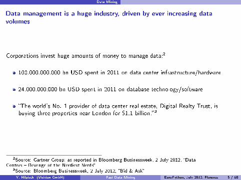
Data management is a huge industry, driven by ever increasing datavolumes
Corporations invest huge amounts of money to manage data:2
100.000.000.000 bn USD spent in 2011 on data center infrastructure/hardware
24.000.000.000 bn USD spent in 2011 on database technology/software
�The world's No. 1 provider of data center real estate, Digital Realty Trust, isbuying three properties near London for $1.1 billion.�3
2Source: Gartner Group; as reported in Bloomberg Businessweek, 2 July 2012, �DataCenters � Revenge of the Nerdiest Nerds�
3Source: Bloomberg Businessweek, 2 July 2012, �Bid & Ask�
Y. Hilpisch (Visixion GmbH) Fast Data Mining EuroPython, July 2012, Florence 5 / 60

Data Mining
Fast Data Mining =
Rapid Implementation
+ Quick Execution
Y. Hilpisch (Visixion GmbH) Fast Data Mining EuroPython, July 2012, Florence 6 / 60

Data Mining
In practice, what we talk about could somehow look like this
Recent question in client project: �How bene�cial are costly guarantees inunit-linked insurance polices from a policy holder perspective?�
Reframed question: �How often would a policy holder would have lost money with10-/15-/20-years straight and mixed savings plans in popular stock indices?�
Solution: Concise Python script�using mainly pandas�to e�ciently analyze thequestion for di�erent parametrizations and with real, i.e. historic, �nancial marketdata.
E�ort (for �rst prototype): Approximately one hour coding and testing (= playing);one hour for preparing a brief presentation with selected results (text + graphics).
Y. Hilpisch (Visixion GmbH) Fast Data Mining EuroPython, July 2012, Florence 7 / 60

Data Mining
Major problems in data management and analysis
sources: data typically comes from di�erent sources, like from the Web, fromin-house databases or it is generated in-memory
formats: data typically comes in di�erent formats, like SQL databases/tables, Excel�les, CSV �les, NumPy arrays
structure: data typically comes di�erently structured, like unstructured, simplyindexed, hierarchically indexed, in table form, in matrix form, in multidimensionalarrays
completeness: real-world data typically comes in an incomplete form, i.e. there ismissing data (e.g. along an index)
convention: for some types of data there a many conventions with regard toformatting, like for dates and time
interpretation: some data sets typically contain information that can be intelligentlyinterpreted, like a time index
performance: reading, streamlining, aligning, analyzing (large) data sets might beslow
Y. Hilpisch (Visixion GmbH) Fast Data Mining EuroPython, July 2012, Florence 8 / 60

Data Mining
What this talk is about
We will talk mainly about two libraries
pandas: a library that conveniently enhances Python's data management andanalysis capabilities; its major focus are in-memory operations
PyTables: a popular database which optimizes writing, reading and analyzing largedata sets out-of-memory, i.e. on disk
We will illustrate their use mainly be the means of examples
Introductory pandas Example�illustration of some fundamental pandas classes andtheir methods
Financial Data Mining in Action�simple, but real world, example
High-Frequency Financial Data�reading and analyzing high-frequency �nancialdata with pandas
Introductory PyTables Example�illustration of some fundamental pandas classesand their methods
Out-Of-Memory Monte Carlo Simulation�implementing a Monte Carlo simulationwith PyTables out-of-memory
Y. Hilpisch (Visixion GmbH) Fast Data Mining EuroPython, July 2012, Florence 9 / 60

Data Mining
Throughout the talk: Results matter more than Style
Bruce Lee�The Tao of Jeet Kune Do:
�There is no mystery about my style. My movements are simple, direct and
non-classical. The extraordinary part of it lies in its simplicity. Every movement
in Jeet Kune Do is being so of itself. There is nothing arti�cial about it. I
always believe that the easy way is the right way.�
The Tao of My Python:
�There is no mystery about my style. My lines of code are simple, direct and
non-classical. The extraordinary part of it lies in its simplicity. Every line of
code in my Python is being so of itself. There is nothing arti�cial about it. I
always believe that the easy way is the right way.�
Y. Hilpisch (Visixion GmbH) Fast Data Mining EuroPython, July 2012, Florence 10 / 60
Some pandas Fundamentals Series class
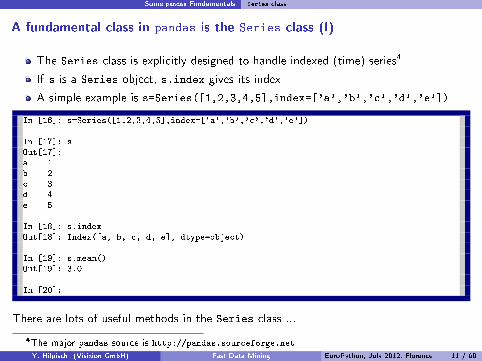
A fundamental class in pandas is the Series class (I)
The Series class is explicitly designed to handle indexed (time) series4
If s is a Series object, s.index gives its index
A simple example is s=Series([1,2,3,4,5],index=['a','b','c','d','e'])
1 In [16]: s=Series([1,2,3,4,5],index=['a','b','c','d','e'])2
3 In [17]: s4 Out[17]:5 a 16 b 27 c 38 d 49 e 5
10
11 In [18]: s.index12 Out[18]: Index([a, b, c, d, e], dtype=object)13
14 In [19]: s.mean()15 Out[19]: 3.016
17 In [20]:
There are lots of useful methods in the Series class ...
4The major pandas source is http://pandas.sourceforge.net
Y. Hilpisch (Visixion GmbH) Fast Data Mining EuroPython, July 2012, Florence 11 / 60

Some pandas Fundamentals Series class
A fundamental class in pandas is the Series class (II)
A major strength of pandas is the handling of time series data, i.e. data indexed bydates and times
An simple example using the DateRange function shall illustrate the time seriesmanagement
1 In [3]: x=standard_normal(250)2
3 In [4]: index=DateRange('01/01/2012',periods=len(x))4
5 In [5]: s=Series(x,index=index)6
7 In [6]: s8 Out[6]:9 2012-01-02 1.06959238875
10 2012-01-03 0.79451540724511 2012-01-04 -1.0159053440412 2012-01-05 -0.75161858882413 ...
Y. Hilpisch (Visixion GmbH) Fast Data Mining EuroPython, July 2012, Florence 12 / 60

Some pandas Fundamentals Series class
The offset parameter of the DateRange function allows �exible, automaticindexing
1 In [33]: datetools.2 datetools.bday datetools.Minute3 datetools.BDay datetools.monthEnd4 datetools.bmonthEnd datetools.MonthEnd5 datetools.BMonthEnd datetools.normalize_date6 datetools.bquarterEnd datetools.ole2datetime7 datetools.BQuarterEnd datetools.OLE_TIME_ZERO8 datetools.businessDay datetools.parser9 datetools.businessMonthEnd datetools.relativedelta
10 datetools.byearEnd datetools.Second11 datetools.BYearEnd datetools.thisBMonthEnd12 datetools.CacheableOffset datetools.thisBQuarterEnd13 datetools.calendar datetools.thisMonthEnd14 datetools.DateOffset datetools.thisYearBegin15 datetools.datetime datetools.thisYearEnd16 datetools.day datetools.Tick17 datetools.format datetools.timedelta18 datetools.getOffset datetools.to_datetime19 datetools.getOffsetName datetools.v20 datetools.hasOffsetName datetools.week21 datetools.Hour datetools.Week22 datetools.i datetools.weekday23 datetools.inferTimeRule datetools.WeekOfMonth24 datetools.isBMonthEnd datetools.yearBegin25 datetools.isBusinessDay datetools.YearBegin26 datetools.isMonthEnd datetools.yearEnd27 datetools.k datetools.YearEnd28
29 In [33]: index=DateRange('01/01/2012',periods=len(x),offset=datetools.DateOffset(2))30
Y. Hilpisch (Visixion GmbH) Fast Data Mining EuroPython, July 2012, Florence 13 / 60

Some pandas Fundamentals DataFrame class
Another fundamental class in pandas is DataFrame
This class's intellectual father is the data.frame class from the statisticallanguage/package R
The DataFrame class is explicitly designed to handle multiple, maybe hierarchicallyindexed (time) series
The following example illustrates some convenient features of the DataFrame class,i.e. data alignment and handling of missing data
1 In [35]: s=Series(standard_normal(4),index=['1','2','3','5'])2
3 In [36]: t=Series(standard_normal(4),index=['1','2','3','4'])4
5 In [37]: df=DataFrame({'s':s,'t':t})6
7 In [38]: df['SUM']=df['s']+df['t']8
9 In [39]: print df.to_string()10 s t SUM11 1 -0.125697 0.016357 -0.10934012 2 0.135457 -0.907421 -0.77196413 3 1.549149 -0.599659 0.94949114 4 NaN 0.734753 NaN15 5 -1.236310 NaN NaN16
17 In [40]: df['SUM'].mean()18 Out[40]: 0.022728863312009556
Y. Hilpisch (Visixion GmbH) Fast Data Mining EuroPython, July 2012, Florence 14 / 60
Some pandas Fundamentals Plotting
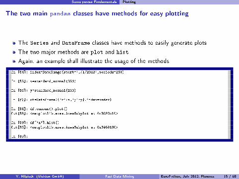
The two main pandas classes have methods for easy plotting
The Series and DataFrame classes have methods to easily generate plots
The two major methods are plot and hist
Again, an example shall illustrate the usage of the methods
1 In [54]: index=DateRange(start='1/1/2013',periods=250)2
3 In [55]: x=standard_normal(250)4
5 In [56]: y=standard_normal(250)6
7 In [57]: df=DataFrame({'x':x,'y':y},index=index)8
9 In [58]: df.cumsum().plot()10 Out[58]: <matplotlib.axes.AxesSubplot at 0x3082c10>11
12 In [59]: df['x'].hist()13 Out[59]: <matplotlib.axes.AxesSubplot at 0x3468190>14
15 In [60]:
Y. Hilpisch (Visixion GmbH) Fast Data Mining EuroPython, July 2012, Florence 15 / 60
Some pandas Fundamentals Plotting
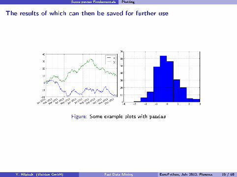
The results of which can then be saved for further use
Figure: Some example plots with pandas
Y. Hilpisch (Visixion GmbH) Fast Data Mining EuroPython, July 2012, Florence 16 / 60

Financial Data Mining in Action
The �rst `real' example should give an impression of the e�ciency ofworking with pandas
1 data gathering: read historical quotes of the Apple stock (ticker AAPL) beginningwith 01 January 2006 from finance.yahoo.com and store it in a pandas
DataFrame object
2 data analysis: calculate the daily log returns (use the shift method of the pandas
Series object) and generate a new column with the log returns in the DataFrame
object
3 plotting: plot the log returns together with the daily Apple quotes into a single �gure
4 simulation: simulate the Apple stock price developement using the last Close quoteas starting value and the historical yearly volatility of the Apple stock (short rate2.5%)�the di�erence equation is given, for s = t−∆t and zt standard normal, by
St = Ss · exp((r − σ2/2)∆t+ σ√
∆tzt)
5 option valuation: calculate the value of a European call option with strike of 110%of the last Close quote and time-to-maturity of 1 year
6 data storage: save the pandas Data Frame to a PyTables/HDF5 database (use theHDFStore function)
Y. Hilpisch (Visixion GmbH) Fast Data Mining EuroPython, July 2012, Florence 17 / 60
Financial Data Mining in Action
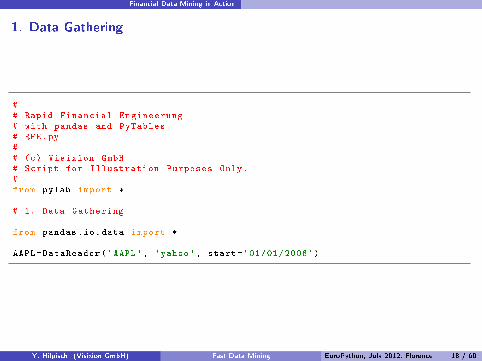
1. Data Gathering
## Rapid Financial Engineerung# with pandas and PyTables# RFE.py## (c) Visixion GmbH# Script for Illustration Purposes Only.#from pylab import *
# 1. Data Gathering
from pandas.io.data import *
AAPL=DataReader('AAPL', 'yahoo ', start='01/01/2006')
Y. Hilpisch (Visixion GmbH) Fast Data Mining EuroPython, July 2012, Florence 18 / 60

Financial Data Mining in Action
2. Data Analysis (I)
# 2. Data Analysis
from pandas import *
AAPL['Ret']=log(AAPL['Close ']/AAPL['Close '].shift(1))
Y. Hilpisch (Visixion GmbH) Fast Data Mining EuroPython, July 2012, Florence 19 / 60
Financial Data Mining in Action
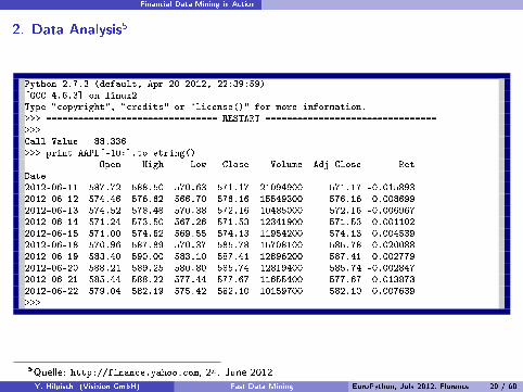
2. Data Analysis5
1 Python 2.7.3 (default, Apr 20 2012, 22:39:59)2 [GCC 4.6.3] on linux23 Type "copyright", "credits" or "license()" for more information.4 >>> ================================ RESTART ================================5 >>>6 Call Value 88.3367 >>> print AAPL[-10:].to_string()8 Open High Low Close Volume Adj Close Ret9 Date
10 2012-06-11 587.72 588.50 570.63 571.17 21094900 571.17 -0.01589311 2012-06-12 574.46 576.62 566.70 576.16 15549300 576.16 0.00869912 2012-06-13 574.52 578.48 570.38 572.16 10485000 572.16 -0.00696713 2012-06-14 571.24 573.50 567.26 571.53 12341900 571.53 -0.00110214 2012-06-15 571.00 574.62 569.55 574.13 11954200 574.13 0.00453915 2012-06-18 570.96 587.89 570.37 585.78 15708100 585.78 0.02008816 2012-06-19 583.40 590.00 583.10 587.41 12896200 587.41 0.00277917 2012-06-20 588.21 589.25 580.80 585.74 12819400 585.74 -0.00284718 2012-06-21 585.44 588.22 577.44 577.67 11655400 577.67 -0.01387319 2012-06-22 579.04 582.19 575.42 582.10 10159700 582.10 0.00763920 >>>
5Quelle: http://finance.yahoo.com, 24. June 2012
Y. Hilpisch (Visixion GmbH) Fast Data Mining EuroPython, July 2012, Florence 20 / 60

Financial Data Mining in Action
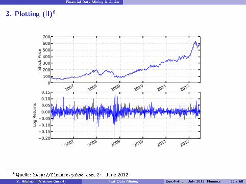
3. Plotting (I)
# 3. Plotting
subplot(211)AAPL['Close '].plot()ylabel('Index Level')
subplot(212)AAPL['Ret'].plot()ylabel('Log Returns ')
Y. Hilpisch (Visixion GmbH) Fast Data Mining EuroPython, July 2012, Florence 21 / 60
Financial Data Mining in Action
3. Plotting (II)6
20072008
20092010
20112012
0
100
200
300
400
500
600
700Sto
ck P
rice
20072008
20092010
20112012
0.20
0.15
0.10
0.05
0.00
0.05
0.10
0.15
Log R
etu
rns
6Quelle: http://finance.yahoo.com, 24. June 2012
Y. Hilpisch (Visixion GmbH) Fast Data Mining EuroPython, July 2012, Florence 22 / 60
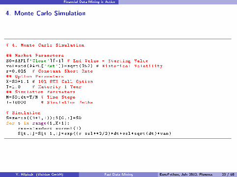
Financial Data Mining in Action
4. Monte Carlo Simulation
# 4. Monte Carlo Simulation
## Market ParametersS0=AAPL['Close '][-1] # End Value = Starting Valuevol=std(AAPL['Ret'])* sqrt(252) # Historical Volatilityr=0.025 # Constant Short Rate## Option ParametersK=S0*1.1 # 10% OTM Call OptionT=1.0 # Maturity 1 Year## Simulation ParametersM=50;dt=T/M # Time StepsI=10000 # Simulation Paths
# SimulationS=zeros((M+1,I));S[0,:]=S0for t in range(1,M+1):
ran=standard_normal(I)S[t,:]=S[t-1,:]* exp((r-vol**2/2)*dt+vol*sqrt(dt)*ran)
Y. Hilpisch (Visixion GmbH) Fast Data Mining EuroPython, July 2012, Florence 23 / 60
Financial Data Mining in Action
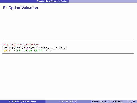
5. Option Valuation
# 5. Option ValuationV0=exp(-r*T)*sum(maximum(S[-1]-K,0))/Iprint "Call Value %8.3f" %V0
Y. Hilpisch (Visixion GmbH) Fast Data Mining EuroPython, July 2012, Florence 24 / 60
Financial Data Mining in Action
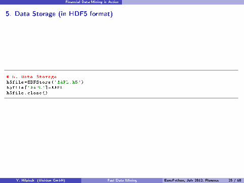
5. Data Storage (in HDF5 format)
# 5. Data Storageh5file=HDFStore('AAPL.h5')h5file['AAPL']=AAPLh5file.close ()
Y. Hilpisch (Visixion GmbH) Fast Data Mining EuroPython, July 2012, Florence 25 / 60

Financial Data Mining in Action
The whole Python script
...from pylab import *# 1. Data Gatheringfrom pandas.io.data import *AAPL=DataReader('AAPL', 'yahoo ', start='01/01/2006')
# 2. Data Analysisfrom pandas import *AAPL['Ret']=log(AAPL['Close ']/AAPL['Close '].shift(1))
# 3. Plottingsubplot(211)AAPL['Close '].plot (); ylabel('Index Level ')subplot(212)AAPL['Ret'].plot (); ylabel('Log Returns ')
# 4. Monte Carlo SimulationS0=AAPL['Close '][-1]vol=std(AAPL['Ret'])* sqrt(252)r=0.025; K=S0*1.1; T=1.0; M=50; dt=T/M; I=10000S=zeros ((M+1,I));S[0,:]=S0for t in range(1,M+1):
ran=standard_normal(I)S[t,:]=S[t-1,:]* exp((r-vol**2/2)*dt+vol*sqrt(dt)*ran)
# 5. Option ValuationV0=exp(-r*T)*sum(maximum(S[-1]-K,0))/Iprint "Call Value %8.3f" %V0
# 6. Data Storageh5file=HDFStore('AAPL.h5'); h5file['AAPL']=AAPL;h5file.close ()
Y. Hilpisch (Visixion GmbH) Fast Data Mining EuroPython, July 2012, Florence 26 / 60
High-Frequency Financial Data
This example is about high-frequency stock data
In this example, we are going to analyze intraday stock price data for Apple (tickerAAPL) and Google (ticker GOOG)
Intraday data for US stocks is available from Netfonds (http://www.netfonds.no),a Norwegian online stock broker
We retrieve intraday data for both stocks for 22 June 2012 as a CSV �le
The Apple stock price data �le contains 16,465 rows; the Google stock price data�le only 7,937 rows
Y. Hilpisch (Visixion GmbH) Fast Data Mining EuroPython, July 2012, Florence 27 / 60
High-Frequency Financial Data
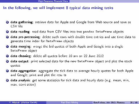
In the following, we will implement 8 typical data mining tasks
1 data gathering: retrieve data for Apple and Google from Web source and save asCSV �le
2 data reading: read data from CSV �les into two pandas DataFrame objects
3 data pre-processing: delete such rows with double time entries and use time data togenerate time index for DataFrame objects
4 data merging: merge the bid quotes of both Apple and Google into a singleDataFrame object
5 data cleaning: delete all quotes before 10 am on 22 June 2012
6 data output: print selected data for the new DataFrame object and plot the stockquotes
7 data aggregation: aggregate the tick data to average hourly quotes for both Appleand Google; print and plot the results
8 data analysis: get some statistics for tick data and hourly data (e.g. mean, min,max, correlation)
Y. Hilpisch (Visixion GmbH) Fast Data Mining EuroPython, July 2012, Florence 28 / 60
High-Frequency Financial Data
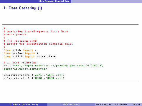
1. Data Gathering (I)
## Analyzing High -Frequency Stock Data# with pandas## (c) Visixion GmbH# Script for illustration purposes only.#from pylab import *from pandas import *from urllib import urlretrieve
# 1. Data Gatheringurl='http :// hopey.netfonds.no/posdump.php?date=20120622 &\paper =%s.O&csv_format=csv'
urlretrieve(url %'AAPL','AAPL.csv')urlretrieve(url %'GOOG','GOOG.csv')
Y. Hilpisch (Visixion GmbH) Fast Data Mining EuroPython, July 2012, Florence 29 / 60
High-Frequency Financial Data
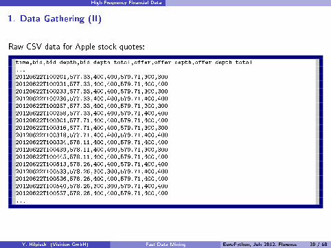
1. Data Gathering (II)
Raw CSV data for Apple stock quotes:
1 time,bid,bid_depth,bid_depth_total,offer,offer_depth,offer_depth_total2 ...3 20120622T100201,577.33,400,400,579.71,300,3004 20120622T100231,577.33,400,400,579.71,400,4005 20120622T100233,577.33,400,400,579.71,300,3006 20120622T100236,577.33,400,400,579.71,400,4007 20120622T100257,577.33,400,400,579.71,300,3008 20120622T100258,577.33,400,400,579.71,400,4009 20120622T100301,577.71,400,400,579.71,400,400
10 20120622T100316,577.71,400,400,579.71,300,30011 20120622T100318,577.71,400,400,579.71,400,40012 20120622T100334,578.11,400,400,579.71,400,40013 20120622T100439,578.11,400,400,579.71,300,30014 20120622T100445,578.11,400,400,579.71,400,40015 20120622T100513,578.26,400,400,579.71,400,40016 20120622T100533,578.26,300,300,579.71,400,40017 20120622T100536,578.26,400,400,579.71,400,40018 20120622T100540,578.26,300,300,579.71,400,40019 20120622T100557,578.26,400,400,579.71,400,40020 ...
Y. Hilpisch (Visixion GmbH) Fast Data Mining EuroPython, July 2012, Florence 30 / 60
High-Frequency Financial Data
2. Data Reading
# 2. Data ReadingAAPL = read_csv('AAPL.csv')GOOG = read_csv('GOOG.csv')
Y. Hilpisch (Visixion GmbH) Fast Data Mining EuroPython, July 2012, Florence 31 / 60

High-Frequency Financial Data
3. Data Pre-Processing (I)
# 3. Data Pre -ProcessingAAPL=AAPL.drop_duplicates(cols='time')GOOG=GOOG.drop_duplicates(cols='time')for i in AAPL.index:
AAPL['time'][i]= datetime.strptime(AAPL['time'][i],'%Y%m%dT%H%M%S')AAPL.index=AAPL['time']; del AAPL['time']for i in GOOG.index:
GOOG['time'][i]= datetime.strptime(GOOG['time'][i],'%Y%m%dT%H%M%S')GOOG.index=GOOG['time']; del GOOG['time']
Y. Hilpisch (Visixion GmbH) Fast Data Mining EuroPython, July 2012, Florence 32 / 60

High-Frequency Financial Data
3. Data Pre-Processing (II)
1 print AAPL[['bid','offer']].ix[1000:1015].to_string()2 bid offer3 time4 2012-06-22 13:57:09 578.71 579.505 2012-06-22 13:57:16 578.71 579.486 2012-06-22 13:57:22 578.72 579.487 2012-06-22 13:57:47 578.73 579.488 2012-06-22 13:57:51 578.74 579.489 2012-06-22 13:57:52 578.75 579.48
10 2012-06-22 13:57:56 578.51 579.4811 2012-06-22 13:57:57 578.53 579.4812 2012-06-22 13:57:59 578.51 579.4813 2012-06-22 13:58:20 578.51 579.4614 2012-06-22 13:58:33 578.75 579.4615 2012-06-22 13:58:36 578.76 579.4616 2012-06-22 13:58:37 578.75 579.4617 2012-06-22 13:58:51 578.76 579.4618 2012-06-22 13:59:29 578.76 579.46
Y. Hilpisch (Visixion GmbH) Fast Data Mining EuroPython, July 2012, Florence 33 / 60
High-Frequency Financial Data
4. Data Merging
# 4. Data MergingDATA = DataFrame({'AAPL': AAPL['bid'],'GOOG': GOOG['bid']})
Y. Hilpisch (Visixion GmbH) Fast Data Mining EuroPython, July 2012, Florence 34 / 60

High-Frequency Financial Data
5. Data Cleaning
# 5. Data CleaningDATA = DATA[DATA.index > datetime(2012 ,06,22 ,9,59,0)]
Y. Hilpisch (Visixion GmbH) Fast Data Mining EuroPython, July 2012, Florence 35 / 60

High-Frequency Financial Data
6. Data Output (I)
# 6. Data Outputprint DATA.ix[:20]. to_string ()DATA.plot(subplots=True)
Y. Hilpisch (Visixion GmbH) Fast Data Mining EuroPython, July 2012, Florence 36 / 60

High-Frequency Financial Data
6. Data Output (II)
1 print AAPL[['bid','offer']].ix[1000:1015].to_string()2 AAPL GOOG3 2012-06-22 10:02:01 577.33 566.34 2012-06-22 10:02:31 577.33 NaN5 2012-06-22 10:02:33 577.33 NaN6 2012-06-22 10:02:36 577.33 NaN7 2012-06-22 10:02:57 577.33 NaN8 2012-06-22 10:02:58 577.33 NaN9 2012-06-22 10:03:01 577.71 NaN
10 2012-06-22 10:03:16 577.71 NaN11 2012-06-22 10:03:18 577.71 NaN12 2012-06-22 10:03:34 578.11 NaN13 2012-06-22 10:04:39 578.11 NaN14 2012-06-22 10:04:45 578.11 NaN15 2012-06-22 10:05:13 578.26 NaN16 2012-06-22 10:05:33 578.26 NaN17 2012-06-22 10:05:36 578.26 NaN18 2012-06-22 10:05:40 578.26 NaN19 2012-06-22 10:05:57 578.26 NaN20 2012-06-22 10:06:00 578.26 NaN21 2012-06-22 10:06:07 578.26 NaN22 2012-06-22 10:06:12 578.26 NaN
Y. Hilpisch (Visixion GmbH) Fast Data Mining EuroPython, July 2012, Florence 37 / 60

High-Frequency Financial Data
6. Data Output (III)7
575576
577578
579
580
581
582
583
AAPL
11:00:00
12:00:00
13:00:00
14:00:00
15:00:00
16:00:00
17:00:00
18:00:00
19:00:00
20:00:00
21:00:00
22:00:00565
566
567
568
569
570
571
572
GOOG
7Quelle: http://finance.yahoo.com, 24. June 2012
Y. Hilpisch (Visixion GmbH) Fast Data Mining EuroPython, July 2012, Florence 38 / 60

High-Frequency Financial Data
7. Data Aggregation (I)
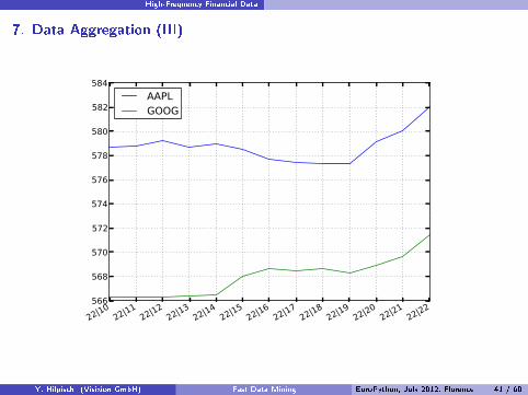
# 7. Data Aggregationby = lambda x: lambda y: getattr(y, x)D = DATA.groupby ([by('day'), by('hour')]). mean()print D; D.plot()
Y. Hilpisch (Visixion GmbH) Fast Data Mining EuroPython, July 2012, Florence 39 / 60

High-Frequency Financial Data
7. Data Aggregation (II)
1 AAPL GOOG2 key_0 key_13 22 10 578.688760 566.3000004 11 578.758111 566.3000005 12 579.211250 566.3000006 13 578.739874 566.4000007 14 578.973806 566.5217868 15 578.547614 568.0201599 16 577.727252 568.609922
10 17 577.405185 568.51365211 18 577.299690 568.65563212 19 577.302453 568.30873913 20 579.156171 568.95642614 21 580.020014 569.63903315 22 582.090000 571.470000
Y. Hilpisch (Visixion GmbH) Fast Data Mining EuroPython, July 2012, Florence 40 / 60
High-Frequency Financial Data
7. Data Aggregation (III)
22|1022|11
22|1222|13
22|1422|15
22|1622|17
22|1822|19
22|2022|21
22|22566
568
570
572
574
576
578
580
582
584
AAPLGOOG
Y. Hilpisch (Visixion GmbH) Fast Data Mining EuroPython, July 2012, Florence 41 / 60
High-Frequency Financial Data
8. Data Analysis (I)
# 8. Data Analysisprint "\n\nSummary Statistics for Tick Data\n",DATA.describe ()print "\nCorrelation for Tick Data\n",DATA.corr()
print "\n\nSummary Statistics for Hourly Data\n",D.describe ()print "\nCorrelation for Hourly Data\n",D.corr()
Y. Hilpisch (Visixion GmbH) Fast Data Mining EuroPython, July 2012, Florence 42 / 60
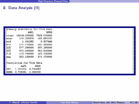
High-Frequency Financial Data
8. Data Analysis (II)
1 Summary Statistics for Tick Data2 AAPL GOOG3 count 14104.000000 7595.0000004 mean 578.320379 568.6821325 std 1.191263 0.9079996 min 575.410000 565.8000007 25% 577.380000 568.1800008 50% 578.400000 568.6400009 75% 579.190000 569.220000
10 max 582.130000 571.47000011
12 Correlation for Tick Data13 AAPL GOOG14 AAPL 1.000000 0.73588415 GOOG 0.735884 1.000000
Y. Hilpisch (Visixion GmbH) Fast Data Mining EuroPython, July 2012, Florence 43 / 60

High-Frequency Financial Data
8. Data Analysis (III)
1 Summary Statistics for Hourly Data2 AAPL GOOG3 count 13.000000 13.0000004 mean 578.763091 567.9996425 std 1.300395 1.5868896 min 577.299690 566.3000007 25% 577.727252 566.4000008 50% 578.739874 568.3087399 75% 579.156171 568.655632
10 max 582.090000 571.47000011
12 Correlation for Hourly Data13 AAPL GOOG14 AAPL 1.000000 0.41735915 GOOG 0.417359 1.000000
Y. Hilpisch (Visixion GmbH) Fast Data Mining EuroPython, July 2012, Florence 44 / 60
Some PyTables Fundamentals Why PyTables and Basic Concepts
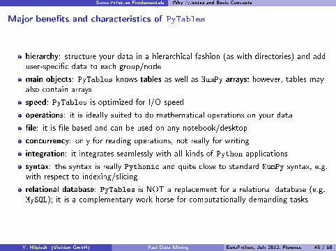
Major bene�ts and characteristics of PyTables
hierarchy: structure your data in a hierarchical fashion (as with directories) and adduser-speci�c data to each group/node
main objects: PyTables knows tables as well as NumPy arrays; however, tables mayalso contain arrays
speed: PyTables is optimized for I/O speed
operations: it is ideally suited to do mathematical operations on your data
�le: it is �le based and can be used on any notebook/desktop
concurrency: only for reading operations, not really for writing
integration: it integrates seamlessly with all kinds of Python applications
syntax: the syntax is really Pythonic and quite close to standard NumPy syntax, e.g.with respect to indexing/slicing
relational database: PyTables is NOT a replacement for a relational database (e.g.MySQL); it is a complementary work horse for computationally demanding tasks
Y. Hilpisch (Visixion GmbH) Fast Data Mining EuroPython, July 2012, Florence 45 / 60
Some PyTables Fundamentals Why PyTables and Basic Concepts
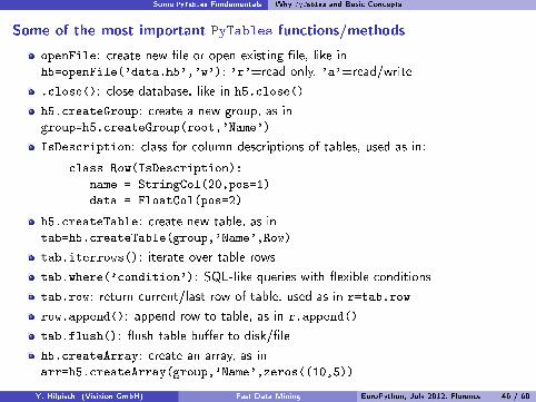
Some of the most important PyTables functions/methods
openFile: create new �le or open existing �le, like inh5=openFile('data.h5','w'); 'r'=read only, 'a'=read/write
.close(): close database, like in h5.close()
h5.createGroup: create a new group, as ingroup=h5.createGroup(root,'Name')
IsDescription: class for column descriptions of tables, used as in:
class Row(IsDescription):
name = StringCol(20,pos=1)
data = FloatCol(pos=2)
h5.createTable: create new table, as intab=h5.createTable(group,'Name',Row)
tab.iterrows(): iterate over table rows
tab.where('condition'): SQL-like queries with �exible conditions
tab.row: return current/last row of table, used as in r=tab.row
row.append(): append row to table, as in r.append()
tab.flush(): �ush table bu�er to disk/�le
h5.createArray: create an array, as inarr=h5.createArray(group,'Name',zeros((10,5))
Y. Hilpisch (Visixion GmbH) Fast Data Mining EuroPython, July 2012, Florence 46 / 60

Some PyTables Fundamentals Introductory PyTables Example
Let's start with a simple example (I)
1 In [59]: from tables import *2
3 In [60]: h5=openFile('Test_Data.h5','w')4
5 In [61]: class Row(IsDescription):6 ....: number = FloatCol(pos=1)7 ....: sqrt = FloatCol(pos=2)8 ....:9
10 In [62]: tab=h5.createTable(h5.root,'Numbers',Row)11
12 In [63]: tab13 Out[63]:14 /Numbers (Table(0,)) ''15 description := {16 "number": Float64Col(shape=(), dflt=0.0, pos=0),17 "sqrt": Float64Col(shape=(), dflt=0.0, pos=1)}18 byteorder := 'little'19 chunkshape := (512,)20
21 In [64]: r=tab.row22
23 In [65]: for x in range(1000):24 ....: r['number']=x25 ....: r['sqrt']=sqrt(x)26 ....: r.append()27 ....:
Y. Hilpisch (Visixion GmbH) Fast Data Mining EuroPython, July 2012, Florence 47 / 60

Some PyTables Fundamentals Introductory PyTables Example
Let's start with a simple example (II)
1 In [66]: tab2 Out[66]:3 /Numbers (Table(0,)) ''4 description := {5 "number": Float64Col(shape=(), dflt=0.0, pos=0),6 "sqrt": Float64Col(shape=(), dflt=0.0, pos=1)}7 byteorder := 'little'8 chunkshape := (512,)9
10 In [67]: tab.flush()11
12 In [68]: tab13 Out[68]:14 /Numbers (Table(1000,)) ''15 description := {16 "number": Float64Col(shape=(), dflt=0.0, pos=0),17 "sqrt": Float64Col(shape=(), dflt=0.0, pos=1)}18 byteorder := 'little'19 chunkshape := (512,)20 In [69]: tab[:5]21 Out[69]:22 array([(0.0, 0.0), (1.0, 1.0), (2.0, 1.4142135623730951),23 (3.0, 1.7320508075688772), (4.0, 2.0)],24 dtype=[('number', '<f8'), ('sqrt', '<f8')])25
26 In [70]:
Y. Hilpisch (Visixion GmbH) Fast Data Mining EuroPython, July 2012, Florence 48 / 60

Some PyTables Fundamentals Introductory PyTables Example
Let's start with a simple example (III)
1 In [7]: h5=openFile('Test_Data.h5','a')2
3 In [8]: h54 Out[8]:5 File(filename=Test_Data.h5, title='', mode='a', rootUEP='/', filters=Filters(complevel=0,6 shuffle=False, fletcher32=False))7 / (RootGroup) ''8 /Numbers (Table(1000,)) ''9 description := {
10 "number": Float64Col(shape=(), dflt=0.0, pos=0),11 "sqrt": Float64Col(shape=(), dflt=0.0, pos=1)}12 byteorder := 'little'13 chunkshape := (512,)14
15
16 In [9]: tab=h5.root.Numbers17
18 In [10]: tab[:5]['sqrt']19 Out[10]: array([ 0. , 1. , 1.41421356, 1.73205081, 2. ])20
21 In [11]: from pylab import *22
23 In [12]: plot(tab[:]['sqrt'])24 Out[12]: [<matplotlib.lines.Line2D at 0x7fe65cf12d10>]25
26 In [13]: show()27
Y. Hilpisch (Visixion GmbH) Fast Data Mining EuroPython, July 2012, Florence 49 / 60
Some PyTables Fundamentals Introductory PyTables Example
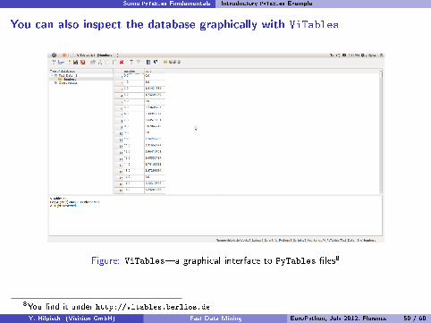
You can also inspect the database graphically with ViTables
Figure: ViTables�a graphical interface to PyTables �les8
8You �nd it under http://vitables.berlios.de
Y. Hilpisch (Visixion GmbH) Fast Data Mining EuroPython, July 2012, Florence 50 / 60
Out-Of-Memory Monte Carlo Simulation
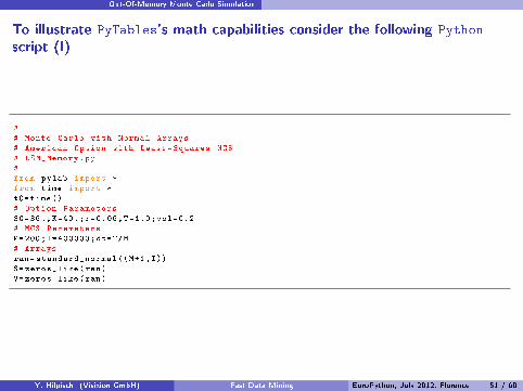
To illustrate PyTables's math capabilities consider the following Python
script (I)
## Monte Carlo with Normal Arrays# American Option with Least -Squares MCS# LSM_Memory.py#from pylab import *from time import *t0=time()# Option ParametersS0=36.;K=40.;r=0.06;T=1.0;vol=0.2# MCS ParametersM=200;I=400000;dt=T/M# Arraysran=standard_normal ((M+1,I))S=zeros_like(ran)V=zeros_like(ran)
Y. Hilpisch (Visixion GmbH) Fast Data Mining EuroPython, July 2012, Florence 51 / 60
Out-Of-Memory Monte Carlo Simulation
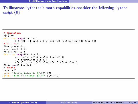
To illustrate PyTables's math capabilities consider the following Python
script (II)
# SimulationS[0]=S0for t in range(1,M+1):
S[t]=S[t-1]*exp((r-0.5*(vol**2))*dt+vol*sqrt(dt)*ran[t])# Valuationdf=exp(-r*dt)h=maximum(K-S,0)V[-1,:]=h[-1,:]for t in range(M-1,0,-1):
rg = polyfit(S[t,:],V[t+1,:]*df ,3)C = polyval(rg,S[t,:])V[t,:] = where(h[t,:]>C,h[t,:],V[t+1,:]*df)
V0=df*sum(V[1 ,:])/I# Outputt1=time()print "Option Value is %7.3f" %V0print "Time in Seconds %7.3f" %(t1 -t0)
Y. Hilpisch (Visixion GmbH) Fast Data Mining EuroPython, July 2012, Florence 52 / 60

Out-Of-Memory Monte Carlo Simulation
With PyTables you can use database objects like NumPy arrays (I)
## Monte Carlo with PyTables Arrays -- Writing and Reading# American Option with Least -Squares MCS# LSM_PyTab.py#from pylab import *from tables import *from time import *t0=time()# Open HDF5 file for Array Storagedata=openFile('LSM_Data.h5','w')# Option ParametersS0=36.;K=40.;r=0.06;T=1.0;vol=0.2# MCS ParametersM=200;I=400000;dt=T/M# Arraysran=data.createArray('/','ran',zeros ((M+1,I),'f'),\
'Random Numbers ')for t in range(M+1):
ran[t]= standard_normal(I)S=data.createArray('/','S',zeros ((M+1,I),'d'),'Index Levels ')h=data.createArray('/','h',zeros ((M+1,I),'d'),'Inner Values ')V=data.createArray('/','V',zeros ((M+1,I),'d'),'Option Values ')C=data.createArray('/','C',zeros ((I),'d'),'Continuation Values ')
Y. Hilpisch (Visixion GmbH) Fast Data Mining EuroPython, July 2012, Florence 53 / 60

Out-Of-Memory Monte Carlo Simulation
With PyTables you can use database objects like NumPy arrays (II)
# SimulationS[0]=S0for t in range(1,M+1):
S[t]=S[t-1]*exp((r-0.5*(vol**2))*dt+vol*sqrt(dt)*ran[t])# Valuationdf=exp(-r*dt)h=maximum(K-S[:,:],0)V[-1,:]=h[-1,:]for t in range(M-1,0,-1):
rg = polyfit(S[t,:],V[t+1,:]*df ,3)C = polyval(rg,S[t,:])V[t,:] = where(h[t,:]>C,h[t,:],V[t+1,:]*df)
V0=df*sum(V[1 ,:])/I# Outputdata.close ();t1=time()print "Option Value is %7.3f" %V0print "Time in Seconds %7.3f" %(t1 -t0)
Y. Hilpisch (Visixion GmbH) Fast Data Mining EuroPython, July 2012, Florence 54 / 60

Out-Of-Memory Monte Carlo Simulation
If you only read from a PyTables database, computations are quite fast
## Monte Carlo with PyTables Array -- Reading from File# American Option with Least -Squares MCS# LSM_PyTab_RO.py#from pylab import *from tables import *from time import *from LSM_PyTab import K,r,T,M,I,dt,dft0=time()# Open HDF5 file for Array Readingdata=openFile('LSM_Data.h5','a')S=data.root.Sh=data.root.hV=data.root.VC=data.root.C# Valuationfor t in range(M-1,0,-1):
rg = polyfit(S[t,:],V[t+1,:]*df ,3)C = polyval(rg,S[t,:])V[t,:] = where(h[t,:]>C,h[t,:],V[t+1,:]*df)
V0=df*sum(V[1 ,:])/I# Outputdata.close ();t1=time()print "Option Value is %7.3f" %V0print "Time in Seconds %7.3f" %(t1 -t0)
Y. Hilpisch (Visixion GmbH) Fast Data Mining EuroPython, July 2012, Florence 55 / 60
Out-Of-Memory Monte Carlo Simulation
In addition, recent versions of PyTables support improved math capabilities
NumPy: fast in-memory array manipulations and operations
numexpr: (memory) improved array operations for faster execution
tables.Expr: combining the strengths of numexpr with PyTables' I/O capabilities
Y. Hilpisch (Visixion GmbH) Fast Data Mining EuroPython, July 2012, Florence 56 / 60
Out-Of-Memory Monte Carlo Simulation
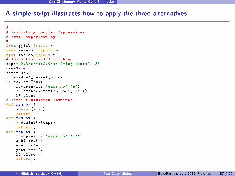
A simple script illustrates how to apply the three alternatives
## Evaluating Complex Expressions# Expr_Comparison.py#from pylab import *from numexpr import *from tables import *# Assumption and Input Dataexpr='0.3*x**3+2.0*x**2+log(abs(x))-3'new=Truesize=10E5x=standard_normal(size)if new == True:
h5=openFile('expr.h5','w')h5.createArray(h5.root ,'x',x)h5.close()
# Three Evaluation Routinesdef num_py ():
y=eval(expr)return y
def num_ex ():y=evaluate(expr)return y
def tab_ex ():h5=openFile('expr.h5','r')x=h5.root.xex=Expr(expr)y=ex.eval()h5.close()return y
Y. Hilpisch (Visixion GmbH) Fast Data Mining EuroPython, July 2012, Florence 57 / 60

Out-Of-Memory Monte Carlo Simulation
Interestingly, reading from HDF5 �le and using Expr is faster than pure NumPy
1 In [43]: %run Expr_Comparison.py2
3 In [44]: %timeit num_py()4 10 loops, best of 3: 177 ms per loop5
6 In [45]: %timeit num_ex()7 100 loops, best of 3: 12.6 ms per loop8
9 In [46]: %timeit tab_ex()10 10 loops, best of 3: 33.3 ms per loop11
12 In [47]: size13 Out[47]: 1000000.014
15 In [48]:16
Y. Hilpisch (Visixion GmbH) Fast Data Mining EuroPython, July 2012, Florence 58 / 60
Out-Of-Memory Monte Carlo Simulation
Visixion's experience with Python
DEXISION: full-�edged Derivatives Analytics suite implemented in Python anddelivered On Demand (since 2006, www.dexision.com)
research: Python used to implement a number of numerical research projects (seewww.visixion.com)
trainings: Python trainings with focus on Finance for clients from the �nancialservices industry
client projects: Python used to implement client speci�c �nancial applications
teaching: Python used to implement and illustrate �nancial models in derivativescourse at Saarland University (see Course Web Site)
talks: we have given a number of talks at Python conferences about the use ofPython for Finance
book: Python used to illustrate �nancial models in our recent book�DerivativesAnalytics with Python�Market-Based Valuation of European and American StockIndex Options�
Y. Hilpisch (Visixion GmbH) Fast Data Mining EuroPython, July 2012, Florence 59 / 60

Out-Of-Memory Monte Carlo Simulation
Contact
Dr. Yves J. HilpischVisixion GmbHRathausstrasse 75-7966333 VoelklingenGermanywww.visixion.com
www.dxevo.com
www.dexision.com
E [email protected] +49 6898 932350
F +49 6898 932352
Y. Hilpisch (Visixion GmbH) Fast Data Mining EuroPython, July 2012, Florence 60 / 60