fast linear discriminant analysis using qr decomposition ...hpark/papers/reglda_ieee.pdf1 fast...

1

Fast Linear Discriminant Analysis using

QR Decomposition and Regularization

Haesun Park, Barry L. Drake, Sangmin Lee, Cheong Hee Park

College of Computing, Georgia Institute of Technology, 266 Ferst Drive, Atlanta, GA 30332, U.S.A.

([email protected], [email protected], [email protected]) The work of the first

three authors was supported in part by the National Science Foundation grants ACI-0305543 and CCF-0621889. Any opinions,

findings and conclusions or recommendations expressed in this material are those of the authors and do not necessarily reflect

the views of the National Science Foundation.

Dept. of Computer Science and Engineering, Chungnam National University, 220 Gung-dong, Yuseong-gu, Daejeon, 305-763,

Korea ([email protected]). The work of this author was supported by the Korea Research Foundation Grant funded

by the Korean Government(MOEHRD)(KRF-2006-331-D00510).

March 23, 2007 DRAFT

2

Abstract

Linear Discriminant Analysis (LDA) is among the most optimal dimension reduction methods for

classification, which provides a high degree of class separability for numerous applications from science

and engineering. However, problems arise with this classical method when one or both of the scatter

matrices is singular. Singular scatter matrices are not unusual in many applications, especially for high-

dimensional data. For high-dimensional undersampled and oversampled problems, the classical LDA

requires modification in order to solve a wider range of problems. In recent work the generalized singular

value decomposition (GSVD) has been shown to mitigate the issue of singular scatter matrices, and a new

algorithm, LDA/GSVD, has been shown to be very robust for many applications in machine learning.

However, the GSVD inherently has a considerable computational overhead. In this paper, we propose fast

algorithms based on the QR decomposition and regularization that solve the LDA/GSVD computational

bottleneck. In addition, we present fast algorithms for classical LDA and regularized LDA utilizing

the framework based on LDA/GSVD and preprocessing by the Cholesky decomposition. Experimental

results are presented that demonstrate substantial speedup in all of classical LDA, regularized LDA, and

LDA/GSVD algorithms without any sacrifice in classification performance for a wide range of machine

learning applications.

Index Terms

Dimension reduction, Linear Discriminant Analysis, Regularization, QR decomposition.

I. INTRODUCTION

Dimension reduction is an important preprocessing step which is encountered in many applica-

tions such as data mining, pattern recognition and scientific visualization. Discovering intrinsic

data structure embedded in high dimensional data can give a low dimensional representation

preserving essential information in the original data. Among several traditional methods, Linear

Discriminant Analysis (LDA) [5] has been known to be one of the most optimal dimension

reduction methods for classification. LDA aims to find an optimal linear transformation that

maximizes the class separability. However, in undersampled problems, where the number of

data samples is smaller than the dimension of the data space, it is difficult to apply classical

LDA due to the singularity of the scatter matrices caused by high dimensionality. In order to make

the LDA applicable in a wider range of applications, several generalizations of the LDA have

been proposed. Among them, a method utilizing the generalized singular value decomposition


3

(GSVD), called LDA/GSVD, has been proposed recently [11], [12] and applied successfully

in various application areas such as text categorization and face recognition. However, one

disadvantage of the classical LDA and its variations for underdetermined systems is their high

computational costs.

In this paper, we address these issues by proposing fast algorithms for classical LDA and

generalizations of LDA such as regularized LDA [4] and LDA/GSVD by taking advantage

of QR decomposition preprocessing and regularization in the framework of the LDA/GSVD

algorithm.

Given a data matrix� ��

, where columns of�

represent data items in an �dimensional space, the problem we consider is that of finding a linear transformation �� that maps a vector � in the � dimensional space to a vector � in the � dimensional space, where

� is an integer with �� , to be determined, based on�

:

� �� (1)

Of special interest in this paper is the case when the data set is already clustered. Our goal is

to find a dimension reducing linear transformation such that the cluster separability of the full

dimensional data matrix�

is preserved in the reduced dimensional space. For this purpose, we

first need to define a measure of cluster quality. When the cluster quality is high, a clustering

result has a tight within-cluster relationship while the between-cluster relationship is remote. In

order to quantify this, in discriminant analysis [5], [21], within-cluster, between-cluster, and total

scatter matrices must be defined. Throughout this paper, for simplicity of discussion, we will

assume that the given data matrix�� !��

is partitioned into " clusters as

�$#�%&� � �(' )*)*) �,+.-where

�,/0�1� �!��3254+6/87 �

/�# 4

9 /denotes the set of column indexes that belong to the cluster : , ;�<

/>=the centroid of each cluster,

and ; the global centroid.

The rest of the paper is organized as followed. In Section II, a brief review of linear dis-

criminant analysis is presented and the formulation of LDA/GSVD is motivated. In Section III,

the generalized singular value decomposition (GSVD) due to Paige and Saunders [15], which

provides a foundation for the fast algorithms we present in this paper, is reviewed. Then the

fast LDA algorithms designed based on the LDA/GSVD framework for undersampled problems


4

utilizing the QR decomposition preprocessing and regularization, as well as for oversampled

problems utilizing the Cholesky decomposition preprocessing [8], are presented in Section IV.

Finally, some substantial experimental results are presented in Section V which illustrates more

than an order of magnitude speedup of the proposed algorithm on many data sets from text

categorization and face recognition.

II. DIMENSION REDUCTION BY LDA

Linear Discriminant Analysis (LDA) is a well known method in the pattern recognition

community for classification and dimension reduction. LDA maximizes the conceptual ratio

of the between-cluster scatter (variance) versus the within-cluster scatter of the data. Here we

provide a brief overview of the basic ideas. For a more in-depth treatment please see [6], [7].

Using the notations introduced in the previous section, the within-cluster scatter matrix �� ,

between-cluster scatter matrix �� , and the total (or mixture) scatter matrix �� are defined as

�� #+6/>7 �

6�� 2

�� ; </>=�� ; <

/>=�� 4 (2)

�� #+6/>7 �

6�� 2

; </>= � ;

� ; </>= � ;

� 4 (3)

and

�� #�6� 7 �

�� ;� �� ;

� 4 (4)

respectively. It is easy to show [5], [9] that the scatter matrices have the relationship

�� # �� (5)

The scatter matrices are analogous to covariance matrices, and are positive semi-definite. Thus,

they can be factored into their "square-root" factors analogous to the case in many signal

processing problems where the covariance matrix is factored into a product of a data matrix

and its transpose [23], [24]. These factors can be used in subsequent processing and circumvent

the condition number squaring problem, since � �(� � # �

' � �.

Thus, we can define the matrices,

� � #�% � � � ; < �=��< �=�� 4 �(' � ; <

' =��<' =�� 43� �3� 4 �,+ � ; <

+ =��<+ =�� - �� 4

(6)

� � # %! � ; < �= � ;

� 4 ' ; <' = � ;

� 43�3�3�54 + ; <+ = � ;

� - �� + 4(7)


5

and � � #�% � � � ; 43�3�3�.4 � � � ; - # � � ;� �� !�� 4 (8)

where�</>= �� 2 ��

and� ��

are vectors where all components are 1’s. Then the scatter

matrices can be expressed as

�� # � � � � 4 �� # � � � � 4 and �� # � � � � � (9)

Note that another way to define� � is

� � # % ; < �= � ;

� �< �= � 4 ; <

' = � ;� �<' = � 43�3�3�.4 ; <

+ = � ;� �<+ = � - �� 4

but the compact form shown in Eqn.(7) reduces the storage requirements and computational

complexity [10], [11].

The measure of the within-cluster scatter can be defined as,

�� ;� ��

� #+6/>7 �

6� � 2

� � �� ; </>= � '' 4

(10)

which is defined over all " clusters, and, similarly, define the measure for between-cluster scatter

as�� ;

� �� #

+6/>7 �

6� � 2

� ; </>= � ; �

'' �(11)

When items within each cluster are located tightly around their own cluster centroid, then

trace( �� ) will have a small value. On the other hand, when the between-cluster relationship

is remote, and hence the centroids of the clusters are remote, trace( �� ) will have a large value.

Using the values trace( �� ), trace( �� ), and Eqn. (5), the cluster quality can be measured. There

are several measures of the overall cluster quality which involve the three scatter matrices [5],

[12], [21], including the maximization of

� � # �� ;� ��

� 4(12)

or� ' # �� ;

� ��

(13)

Note that both of the above criteria require �� to be nonsingular, or equivalently, require� � to

have full rank. For more measures of cluster quality, their relationships, and their extension to

text document data, see [5], [12].


6

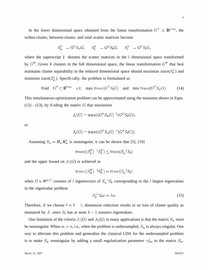
In the lower dimensional space obtained from the linear transformation � � � � ��, the

within-cluster, between-cluster, and total scatter matrices become

� �� # � �� 4 � �� # � �� 4 � �� # � �� 4

where the superscript�

denotes the scatter matrices in the � dimensional space transformed

by � . Given " clusters in the full dimensional space, the linear transformation � that best

maintains cluster separability in the reduced dimensional space should maximize trace( � �� ) and

minimize trace( � �� ). Specifically, the problem is formulated as

Find � �� max

�� ;� � ��

�and min

�� ;� � ��

� �(14)

This simultaneous optimization problem can be approximated using the measures shown in Eqns.

(12) - (13), by finding the matrix � that maximizes

� � �� #

trace � ��

��

� � 4

or� ' �

� #trace

� ��

� � �

Assuming �� # � � � � is nonsingular, it can be shown that [5], [10]

�� ;� � ��

��

�� ;

� � � ��

and the upper bound on� � �

�is achieved as

�� ;� � ��

��

� # �� ;� ��

�

when � � �� consists of � eigenvectors of � � �� corresponding to the � largest eigenvalues

in the eigenvalue problem

�� #�� (15)

Therefore, if we choose � # " �� , dimension reduction results in no loss of cluster quality as

measured by� � since �� has at most " �� nonzero eigenvalues.

One limitation of the criteria� � �

�and

� ' ��

in many applications is that the matrix �� must

be nonsingular. When �� , i.e., when the problem is undersampled, � � is always singular. One

way to alleviate this problem and generalize the classical LDA for the undersampled problem

is to make �� nonsingular by adding a small regularization parameter �� to the matrix �� .


7

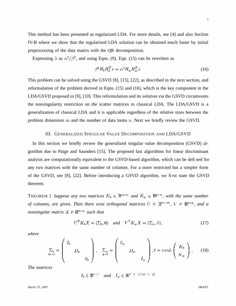
This method has been presented as regularized LDA. For more details, see [4] and also Section

IV-B where we show that the regularized LDA solution can be obtained much faster by initial

preprocessing of the data matrix with the QR decomposition.

Expressing�

as � '�� ' , and using Eqns. (9), Eqn. (15) can be rewritten as� ' � � � � � # � ' � � � � � � (16)

This problem can be solved using the GSVD [8], [15], [22], as described in the next section, and

reformulation of the problem derived in Eqns. (15) and (16), which is the key component in the

LDA/GSVD proposed in [9], [10]. This reformulation and its solution via the GSVD circumvents

the nonsingularity restriction on the scatter matrices in classical LDA. The LDA/GSVD is a

generalization of classical LDA and it is applicable regardless of the relative sizes between the

problem dimension � and the number of data items . Next we briefly review the GSVD.

III. GENERALIZED SINGULAR VALUE DECOMPOSITION AND LDA/GSVD

In this section we briefly review the generalized singular value decomposition (GSVD) al-

gorithm due to Paige and Saunders [15]. The proposed fast algorithms for linear discriminant

analysis are computationally equivalent to the GSVD-based algorithm, which can be defined for

any two matrices with the same number of columns. For a more restricted but a simpler form

of the GSVD, see [8], [22]. Before introducing a GSVD algorithm, we first state the GSVD

theorem:

THEOREM 1 Suppose any two matrices � � � � �!�� and �� , with the same number

of columns, are given. Then there exist orthogonal matrices � � �!�!��, � � � � �

, and a

nonsingular matrix �� such that

� �� # � � 4�� and �� # � � 4�� 4 (17)

where

� ��!� � #��

� � �

�� 4 � �� #

��

��

�� 4 � # � � �"

��

�� (18)

The matrices

� � �� and � � �1� < � � � �� = � < � � � �� =March 23, 2007 DRAFT

8

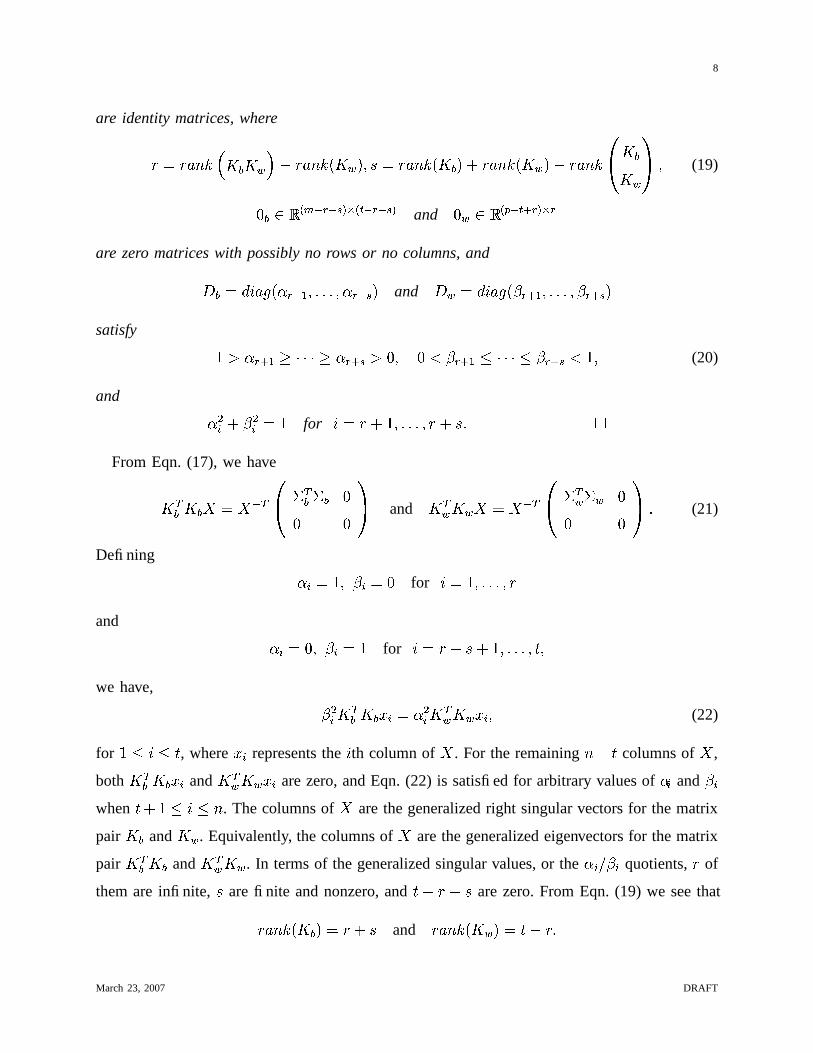
are identity matrices, where

� # � � "�� " � �� 4 � # � � �" � �

�� " � �

� � � � �"��

�� 4(19)

� � �1� < � � � �� = � < � � � �� = and� � �� < � � �� = � �

are zero matrices with possibly no rows or no columns, and�� #�� : �� 4 �3�3�54 � � � �

�and

�� #�� : �� 43�3�3�54 � � � �

�

satisfy

� � � � � �� )*)*) � � � � � � 4 � � � � � � � )*)*) � � � � � � � 4 (20)

and � '/ � � '/ # � for : # � � � 43�3�3�54 � � � � �From Eqn. (17), we have

� � �� # � ��

�� and � � �� # � ��

�� (21)

Defining � /�# � 4 � /�# �for : # � 43�3�3�.4 �

and � /�# � 4 � /�# � for : # � � � � � 43�3�3�54 � 4

we have, � '/ � � �� /�# � '/ � � �� / 4 (22)

for ��:��, where � / represents the : th column of . For the remaining � � columns of ,

both � � �� / and � � � � � / are zero, and Eqn. (22) is satisfied for arbitrary values of � / and� /

when� � �

�:� . The columns of are the generalized right singular vectors for the matrix

pair � � and �� . Equivalently, the columns of are the generalized eigenvectors for the matrix

pair � � � � and � � � � . In terms of the generalized singular values, or the � / �� / quotients,�

of

them are infinite,�

are finite and nonzero, and� � � � � are zero. From Eqn. (19) we see that

� � �" � �� # � � � and

� � �" �� # � � � �


9

� 2 �*2 �32�� 2 belongs to� ��1 0 � null �� null ��! "�#�$��! &% �(' � 2 '&) )+* � 2 *,� � ' � 2 '$) null ��-�� null �� ! �%. "�(��0/0 1 0 null �� null ��/1 2�(��.��3

any value any value any value null �� 1� null ��TABLE I

GENERALIZED EIGENVALUES� 2 ’S AND EIGENVECTORS 2 ’S FROM THE GSVD. THE SUPERSCRIPT 4 DENOTES THE

COMPLEMENT.

Algorithm 1 LDA/GSVDGiven a data matrix

� ��where the columns are partitioned into " clusters, this algorithm

computes the the dimension reducing transformation � �� <+�� =

. For any vector � �� ,� # � � � � <

+�� = ��

gives a " � �

�dimensional representation of � .

1) Compute� � �1��!�

+and

� � �� from�

according to Eqns. (7) and (6), respectively.

2) Compute the complete orthogonal decomposition of � #��

�� <+ � � = �� , i.e.,

5 � #�� 6 ��

�� 4where

5 �� <+ � � = � < + � � = and ��

are orthogonal,

and6

is a square matrix with� � " � � # � � �" 6

�.

3) Let� # � � " � � �

4) Compute W from the SVD of5 � � " 4 � � �

�, i.e., � 5 � � " 4 � � �

�87 # � �5) Compute the first " �� columns of

�� 6�� 7 ��

�� , and assign them to � .

The GSVD algorithm adopted in this paper is based on the constructive proof of the GSVD

presented in Paige and Saunders [15]. The GSVD is a powerful tool not only for algorithm

development, but also for analysis. In Table I, four subspaces of interest spanned by the columns

of X from the GSVD are characterized.

The GSVD has been applied to the matrix pair � � 4 � �

�to find the dimension reducing

transformation for LDA/GSVD, which was first introduced in [10], [11]. The LDA/GSVD method

does not depend on the scatter matrices being nonsingular. The algorithm is summarized in


10

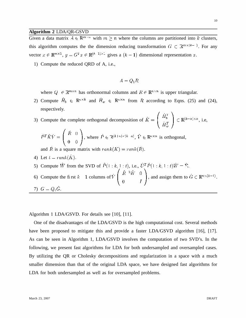
Algorithm 2 LDA/QR-GSVDGiven a data matrix

� �� with � where the columns are partitioned into " clusters,

this algorithm computes the the dimension reducing transformation � � � �� <+�� =

. For any

vector � � � �� , � # � � � � <+�� = ��

gives a " � �

�dimensional representation � .

1) Compute the reduced QRD of A, i.e.,

� #�� 6

where� � ��!�� has orthonormal columns and

6 �� is upper triangular.

2) Compute �� +

and ��

from6

according to Eqns. (25) and (24),

respectively.

3) Compute the complete orthogonal decomposition of �� #��

�� <+ � � = �� , i.e,

�5 �� #

�� 6 �� , where �

5 �� <+ � � = � < + � � = , � � � � ��

is orthogonal,

and �6

is a square matrix with� � �" �� # � � " �6

�.

4) Let� # � � " ��

5) Compute �7

from the SVD of �5 � � " 4 � � �

�, i.e., �� 5 � � " 4 � � �

��7 #

��

6) Compute the first " � � columns of �� 6 � � �7 ��

�� , and assign them to �� <+�� =

.

7) � #�� .

Algorithm 1 LDA/GSVD. For details see [10], [11].

One of the disadvantages of the LDA/GSVD is the high computational cost. Several methods

have been proposed to mitigate this and provide a faster LDA/GSVD algorithm [16], [17].

As can be seen in Algorithm 1, LDA/GSVD involves the computation of two SVD’s. In the

following, we present fast algorithms for LDA for both undersampled and oversampled cases.

By utilizing the QR or Cholesky decompositions and regularization in a space with a much

smaller dimension than that of the original LDA space, we have designed fast algorithms for

LDA for both undersampled as well as for oversampled problems.


11

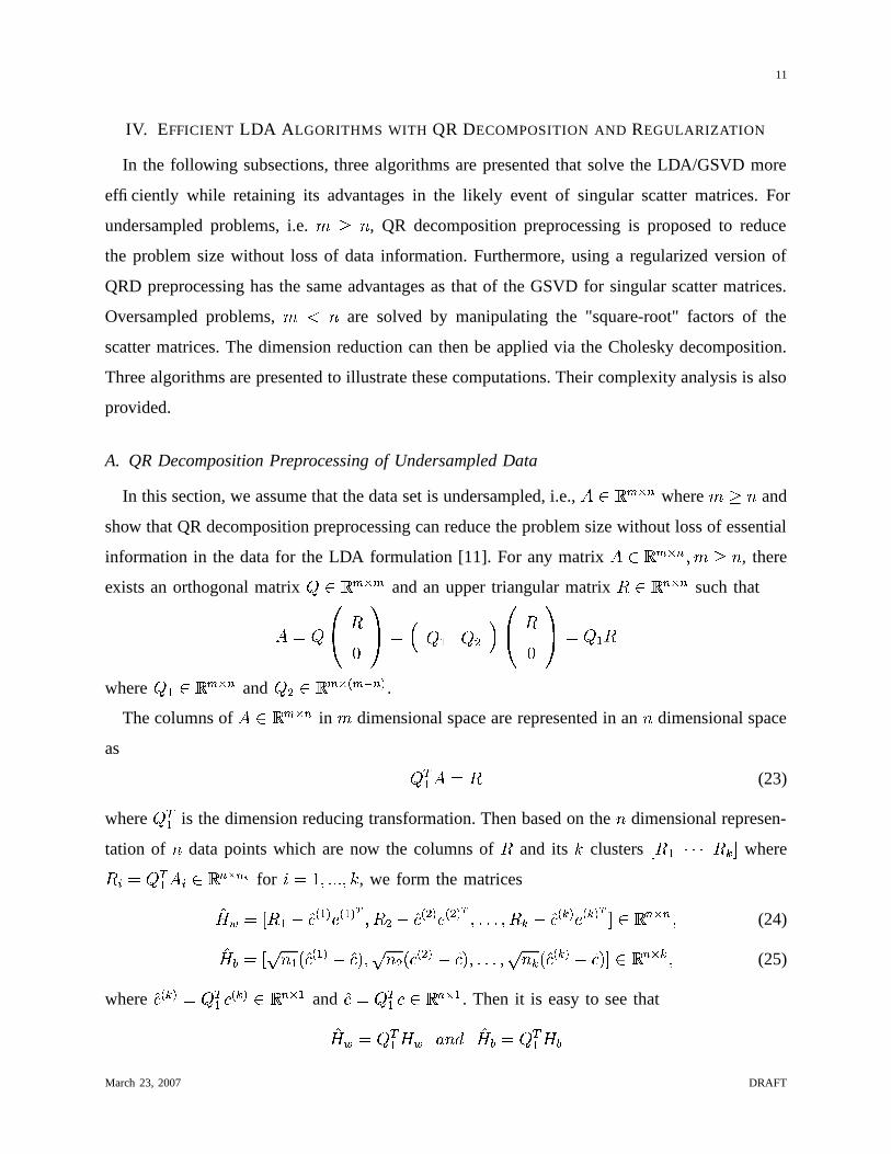
IV. EFFICIENT LDA ALGORITHMS WITH QR DECOMPOSITION AND REGULARIZATION

In the following subsections, three algorithms are presented that solve the LDA/GSVD more

efficiently while retaining its advantages in the likely event of singular scatter matrices. For

undersampled problems, i.e. � , QR decomposition preprocessing is proposed to reduce

the problem size without loss of data information. Furthermore, using a regularized version of

QRD preprocessing has the same advantages as that of the GSVD for singular scatter matrices.

Oversampled problems, � � are solved by manipulating the "square-root" factors of the

scatter matrices. The dimension reduction can then be applied via the Cholesky decomposition.

Three algorithms are presented to illustrate these computations. Their complexity analysis is also

provided.

A. QR Decomposition Preprocessing of Undersampled Data

In this section, we assume that the data set is undersampled, i.e.,��!�!��

where � and

show that QR decomposition preprocessing can reduce the problem size without loss of essential

information in the data for the LDA formulation [11]. For any matrix� �1�!�� 4 � , there

exists an orthogonal matrix��1� ��

and an upper triangular matrix6 ��

such that

� # �� 6 �

�� # � � � � ' �� 6 �

�� # � � 6

where� � �1��!�� and

� ' �� < � � �=.

The columns of� � � ��

in � dimensional space are represented in an dimensional space

as� � � # 6

(23)

where� � is the dimension reducing transformation. Then based on the dimensional represen-

tation of data points which are now the columns of6

and its " clusters% 6 � )*)*) 6 + - where

6 /�#�� ,/ �� 2 for : # � 43� � � 4 " , we form the matrices

�� #�% 6 � � �; < �

= �< �= � 4 6 ' �

�; <' = �<' = � 43� �3� 4 6 + �

�; <+ = �<+ = � - �� 4

(24)

�� # % � �; < �

= ��;� 4 ' �; <

' = ��;� 43�3� � 4 + �; <

+ = ��;� - �� + 4

(25)

where �; <+ = #�� ; <

+ = �� and �; #�� ; � �� . Then it is easy to see that

�� #��

� � # � � � �March 23, 2007 DRAFT

12

With the scatter matrices

�� # �� #�� #�� and (26)

�� # �� # � � � � � � � � #�� 4 (27)

suppose we find a matrix � that minimizes�� ;

� � ��

and maximizes�� ;

� � ��

Then since

� �� #� �� #

� � � � � � � � � � (28)

� �� #� �� #

� � � � � � � � � � (29)

#�� provides the solution for minimizing�� ;

� � ��

and maximizing�� ;

� � �� ,

which is the LDA/GSVD solution shown in Algorithm 1. The discussion above shows that the

preprocessing step by the reduced QR decomposition of�

enables one to solve LDA/GSVD by

manipulating much smaller matrices of size � rather than � � in the case of under-sampled

problems.

Specifically, efficiency in LDA/QR-GSVD (see Algorithm 2) is obtained in step 3 where the

time complexity of� ��

�is sufficient for the complete orthogonal decomposition of the �

matrix, while LDA/GSVD requires� �

'�

with an � � matrix in step 2. For undersampled

problems where the data dimension, � , could be up to several thousands, QR decomposition

preprocessing can produce significant time and memory savings as demonstrated in Section V.

B. Regularization and QRD Preprocessing

When �� is singular or ill conditioned, in regularized LDA a diagonal matrix �� with � �,

is added to �� to make it nonsingular. Regularized LDA has been commonly used for dimension

reduction of high dimensional data in many application areas. However, high dimensionality can

make the time complexity and memory requirements very expensive, since computing the SVD

of the scatter matrices is required for regularized LDA.

We now show that if we apply regularization after preprocessing by the QR decomposition on

the data set, the process of regularization becomes simpler since we work with the within-cluster

scatter matrix, which is transformed into a much smaller dimensional space ( � compared

to � � ). In addition, we will show that though regularization is preceded by preprocessing

of the data matrix�

, it is equivalent to regularized LDA without preprocessing. When this


13

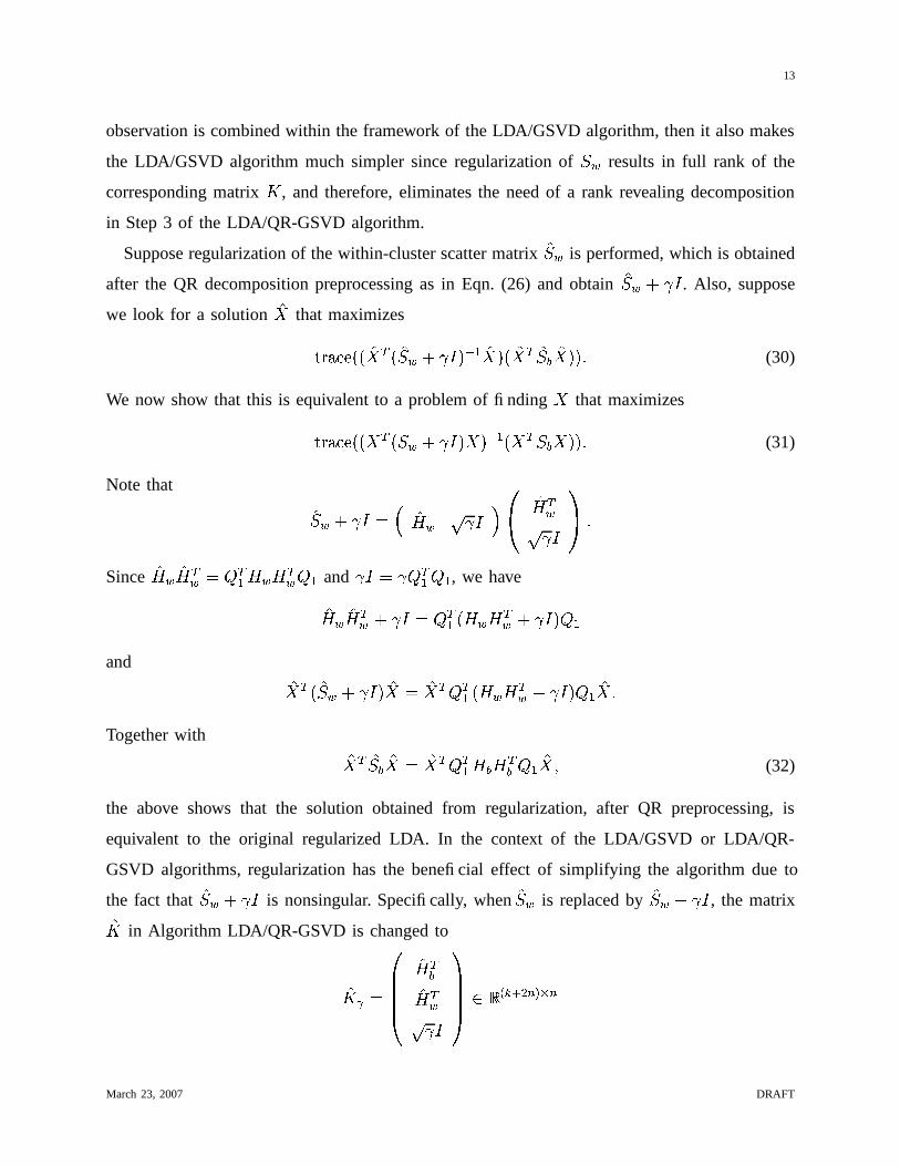
observation is combined within the framework of the LDA/GSVD algorithm, then it also makes

the LDA/GSVD algorithm much simpler since regularization of �� results in full rank of the

corresponding matrix � , and therefore, eliminates the need of a rank revealing decomposition

in Step 3 of the LDA/QR-GSVD algorithm.

Suppose regularization of the within-cluster scatter matrix �� is performed, which is obtained

after the QR decomposition preprocessing as in Eqn. (26) and obtain �� . Also, suppose

we look for a solution � that maximizes

��

��

(30)

We now show that this is equivalent to a problem of finding that maximizes

��

��

(31)

Note that

�� # � ��

� � ��

��

Since �� # � � � � � � � � and �� # � � � � , we have

�� # � � � � � � � ��

��

and

� �� #

� � � � � � � � ��

Together with

� �� #� � � � � � � � � � 4 (32)

the above shows that the solution obtained from regularization, after QR preprocessing, is

equivalent to the original regularized LDA. In the context of the LDA/GSVD or LDA/QR-

GSVD algorithms, regularization has the beneficial effect of simplifying the algorithm due to

the fact that �� is nonsingular. Specifically, when �� is replaced by �� , the matrix

�� in Algorithm LDA/QR-GSVD is changed to

��#

��

� �� <

+ � ' � = ��


14

and� � �" ��

�is full for any value � �

. For this reason we do not have to go through the

process of revealing the rank as in Step 3 of Algorithm 2. Instead, the reduced QR decomposition

of �� will suffice. The new algorithm is presented in Algorithm 3.

Regularization provides another advantage by alleviating the overfitting problem inherent in

LDA/GSVD. When �� is singular and, accordingly,� : � � � � ��

� � � , Table III and

� � � �� #��

�� and � � �� #��

�� (33)

show that the largest generalized eigenvalue is � . The leading generalized eigenvectors that

consist of the first�

columns of give

� �� # �where � �1�� . This means that the within-cluster scatter matrix, after the dimension reducing

transformation by � , becomes zero and accordingly all data points in�

in each cluster are

transformed to the same point. Then the optimal dimension reducing transformation% � ' -

from LDA/GSVD tends to map every point within the same cluster onto an extremely narrow

region of a single point, resulting in�� % � ' - �� % � ' - �� '��

. Since the goal of LDA is

to find a dimension reducing transformation that minimizes the within-cluster relationship and

maximizes the between-cluster relationship, the small norm of the within-cluster scatter matrix

in the reduced dimensional space may seem to be a desirable result. However, such a small norm

of the within-cluster scatter matrix causes difficulties in generalizing test data, and having very

small regions for each cluster will prove detrimental for classification. In order to resolve this

problem, we need to make �� nonsingular by adding a regularization term to �� , such as �� where is a small positive number. This idea of applying regularization to LDA/GSVD may

seem to be identical to regularized LDA. However, within the LDA/GSVD algorithm framework,

QR decomposition preprocessed data and regularization, an algorithm obtained (Algorithm 3) is

significantly more efficient as shown in the numerical experiments, Section V.

C. Fast LDA Algorithm for Oversampled Problems

When the number of data points exceeds the data dimension, QR decomposition preprocessing

becomes useless since the dimension of the upper triangular matrix R will be the same as the

dimension of the original data. The solution to this is arrived at by manipulating the matrix


15

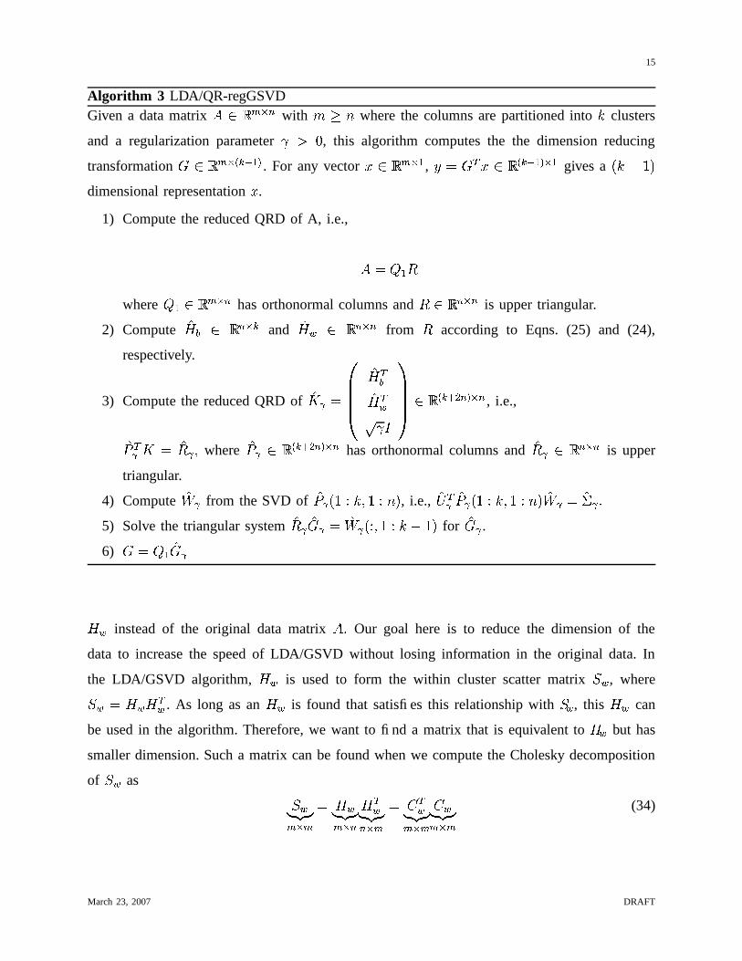
Algorithm 3 LDA/QR-regGSVDGiven a data matrix

� � ��with � where the columns are partitioned into " clusters

and a regularization parameter � �, this algorithm computes the the dimension reducing

transformation � � � �� <+�� =

. For any vector � � � �� , � # � � � � <+�� = ��

gives a " ��

�

dimensional representation � .

1) Compute the reduced QRD of A, i.e.,

� #�� 6

where� � �� !�� has orthonormal columns and

6 �� is upper triangular.

2) Compute �� +

and ��

from6


respectively.

3) Compute the reduced QRD of ��#

��

� �� <

+ � ' � = �� , i.e.,

�5 � #

�64

where �5� � <

+ � ' � = �� has orthonormal columns and �6� ��

is upper

triangular.

4) Compute �7 from the SVD of �

5 � � " 4 � �

�, i.e., �� 5 � � " 4 � � � �7

#��

5) Solve the triangular system �6 �� # �

7 � 4 � � " ��

�for �� .

6) � #��

� � instead of the original data matrix� �

Our goal here is to reduce the dimension of the

data to increase the speed of LDA/GSVD without losing information in the original data. In

the LDA/GSVD algorithm,� � is used to form the within cluster scatter matrix �� , where

�� # � � � � . As long as an� � is found that satisfies this relationship with � � , this

� � can

be used in the algorithm. Therefore, we want to find a matrix that is equivalent to� � but has

smaller dimension. Such a matrix can be found when we compute the Cholesky decomposition

of �� as

��!��# � ��!��

� �� # � ��

� ��!�� (34)


16

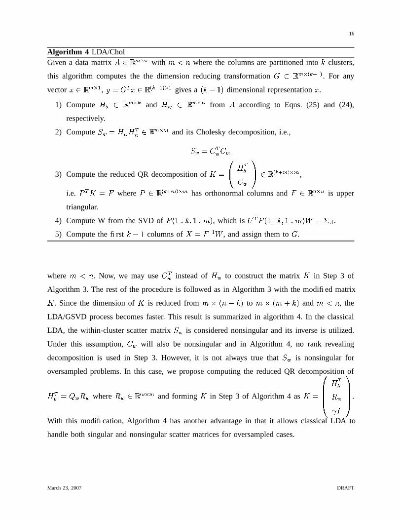
Algorithm 4 LDA/CholGiven a data matrix

� � ��!��with � � where the columns are partitioned into " clusters,

this algorithm computes the the dimension reducing transformation � � � �� <+�� =

. For any

vector � � � �� , � # � � � � <+�� = ��

gives a " � �

�dimensional representation � .

1) Compute� � � � �� +

and� � � � ��

from�


respectively.

2) Compute �� # � � � � �� !�� and its Cholesky decomposition, i.e.,

�� # � � � �

3) Compute the reduced QR decomposition of � #��

��

�� <+ � � = �� ,

i.e.5 � # �

where5 � � <

+ � � = �� has orthonormal columns and� � � � ��

is upper

triangular.

4) Compute W from the SVD of5 � � " 4 � � �

�, which is � 5 � � " 4 � � �

� 7 # �� 5) Compute the first " �� columns of # �

�� 7

, and assign them to � .

where � � . Now, we may use� � instead of

� � to construct the matrix � in Step 3 of

Algorithm 3. The rest of the procedure is followed as in Algorithm 3 with the modified matrix� . Since the dimension of � is reduced from � � �$"�

to � � � � "�

and � � , the

LDA/GSVD process becomes faster. This result is summarized in algorithm 4. In the classical

LDA, the within-cluster scatter matrix �� is considered nonsingular and its inverse is utilized.

Under this assumption,� � will also be nonsingular and in Algorithm 4, no rank revealing

decomposition is used in Step 3. However, it is not always true that � � is nonsingular for

oversampled problems. In this case, we propose computing the reduced QR decomposition of

� � # � � 6 � where6 � � ��!�� and forming � in Step 3 of Algorithm 4 as � #

�� 6 � �

� �� .

With this modification, Algorithm 4 has another advantage in that it allows classical LDA to

handle both singular and nonsingular scatter matrices for oversampled cases.


17

TABLE II

DESCRIPTION OF THE DATA SETS USED. THE FIRST FOUR DATA SETS CORRESPOND TO UNDERSAMPLED CASES AND THE

LAST THREE ARE DATA SETS FOR OVERSAMPLED CASES.

Data set number of data dimension number of clusters training test

Text 210 5896 7 168 42

Yale 165 77760 15 135 30

AT � T 400 10304 40 320 80

Feret 130 3000 10 100 30

ImageSeg 2310 19 7 2100 210

Optdigit 5610 64 10 3813 1797

Isolet 7797 617 26 6238 1559

V. EXPERIMENTAL RESULTS

We have tested the proposed algorithms on undersampled problems as well as oversampled

problems. For the undersampled case, regularized LDA, LDA/GSVD, LDA/QR-GSVD, and

LDA/QR-regGSVD are tested using data sets for text categorization and face recognition. For the

oversampled case, LDA/GSVD, LDA/Chol, and classical LDA are tested for various benchmark

data sets from the UCI machine learning repository. A detailed description of the data sets is

given in Table II. All the experiments were run using MATLAB on Windows XP with 1.79 GHz

CPU and 1 GB memory.

The first data set denoted as Text in Table II is for the text categorization problem and

was downloaded from http://www-users.cs.umn.edu/ � karypis/cluto/download.html. This data set

consists of a total 210 instances of documents and 5896 terms. The data set was composed of 7

clusters, each cluster contains 30 data samples. From this data set, ��

’s were used for training,

and the remaining for testing. From the face recognition data, three data sets were used, Yale,

AT � T and Feret face data. The Yale face data consists of 165 images, each image contained

77760 pixels. The data set is made up of 15 clusters and each cluster contains 11 images of the

same person. Out of 165 images, 135 were used for training and 30 were used for testing. The

AT � T and Feret face data, were similarly composed and used in the experiments.

Tables III and IV compare the time complexities and classification accuracies of those algo-

rithms tested on undersampled problems, respectively. For all the methods, k nearest neighbor


18

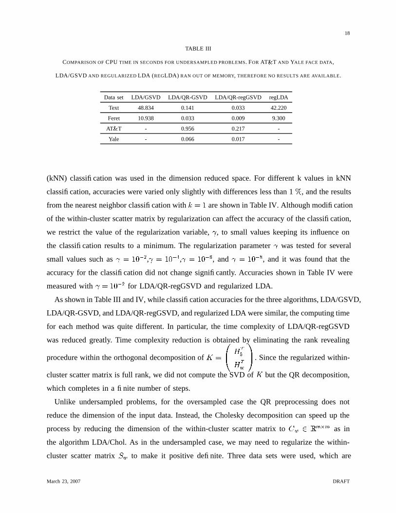
TABLE III

COMPARISON OF CPU TIME IN SECONDS FOR UNDERSAMPLED PROBLEMS. FOR AT � T AND YALE FACE DATA,

LDA/GSVD AND REGULARIZED LDA (REGLDA) RAN OUT OF MEMORY, THEREFORE NO RESULTS ARE AVAILABLE.

Data set LDA/GSVD LDA/QR-GSVD LDA/QR-regGSVD regLDA

Text 48.834 0.141 0.033 42.220

Feret 10.938 0.033 0.009 9.300

AT � T - 0.956 0.217 -

Yale - 0.066 0.017 -

(kNN) classification was used in the dimension reduced space. For different k values in kNN

classification, accuracies were varied only slightly with differences less than 1 � , and the results

from the nearest neighbor classification with " # � are shown in Table IV. Although modification

of the within-cluster scatter matrix by regularization can affect the accuracy of the classification,

we restrict the value of the regularization variable, , to small values keeping its influence on

the classification results to a minimum. The regularization parameter was tested for several

small values such as # � � � ' , # � � �� , # � � �� , and # � � �� , and it was found that the

accuracy for the classification did not change significantly. Accuracies shown in Table IV were

measured with # � � � ' for LDA/QR-regGSVD and regularized LDA.

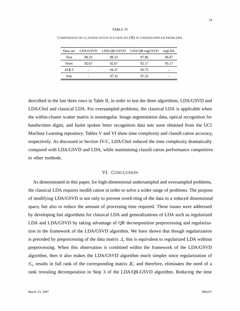
As shown in Table III and IV, while classification accuracies for the three algorithms, LDA/GSVD,

LDA/QR-GSVD, and LDA/QR-regGSVD, and regularized LDA were similar, the computing time

for each method was quite different. In particular, the time complexity of LDA/QR-regGSVD

was reduced greatly. Time complexity reduction is obtained by eliminating the rank revealing

procedure within the orthogonal decomposition of � #��

��

�� . Since the regularized within-

cluster scatter matrix is full rank, we did not compute the SVD of � but the QR decomposition,

which completes in a finite number of steps.

Unlike undersampled problems, for the oversampled case the QR preprocessing does not

reduce the dimension of the input data. Instead, the Cholesky decomposition can speed up the

process by reducing the dimension of the within-cluster scatter matrix to� � � ��!��

as in

the algorithm LDA/Chol. As in the undersampled case, we may need to regularize the within-

cluster scatter matrix �� to make it positive definite. Three data sets were used, which are


19

TABLE IV

COMPARISON OF CLASSIFICATION ACCURACIES ( � ) IN UNDERSAMPLED PROBLEMS.

Data set LDA/GSVD LDA/QR-GSVD LDA/QR-regGSVD regLDA

Text 98.33 98.33 97.86 96.67

Feret 92.67 92.67 92.17 95.17

AT � T - 94.37 93.75 -

Yale - 97.33 97.33 -

described in the last three rows in Table II, in order to test the three algorithms, LDA/GSVD and

LDA/Chol and classical LDA. For oversampled problems, the classical LDA is applicable when

the within-cluster scatter matrix is nonsingular. Image segmentation data, optical recognition for

handwritten digits, and Isolet spoken letter recognition data sets were obtained from the UCI

Machine Learning repository. Tables V and VI show time complexity and classification accuracy,

respectively. As discussed in Section IV-C, LDA/Chol reduced the time complexity dramatically

compared with LDA/GSVD and LDA, while maintaining classification performance competitive

to other methods.

VI. CONCLUSION

As demonstrated in this paper, for high-dimensional undersampled and oversampled problems,

the classical LDA requires modification in order to solve a wider range of problems. The purpose

of modifying LDA/GSVD is not only to prevent overfitting of the data in a reduced dimensional

space, but also to reduce the amount of processing time required. These issues were addressed

by developing fast algorithms for classical LDA and generalizations of LDA such as regularized

LDA and LDA/GSVD by taking advantage of QR decomposition preprocessing and regulariza-

tion in the framework of the LDA/GSVD algorithm. We have shown that though regularization

is preceded by preprocessing of the data matrix�

, this is equivalent to regularized LDA without

preprocessing. When this observation is combined within the framework of the LDA/GSVD

algorithm, then it also makes the LDA/GSVD algorithm much simpler since regularization of

�� results in full rank of the corresponding matrix � , and therefore, eliminates the need of a

rank revealing decomposition in Step 3 of the LDA/QR-GSVD algorithm. Reducing the time


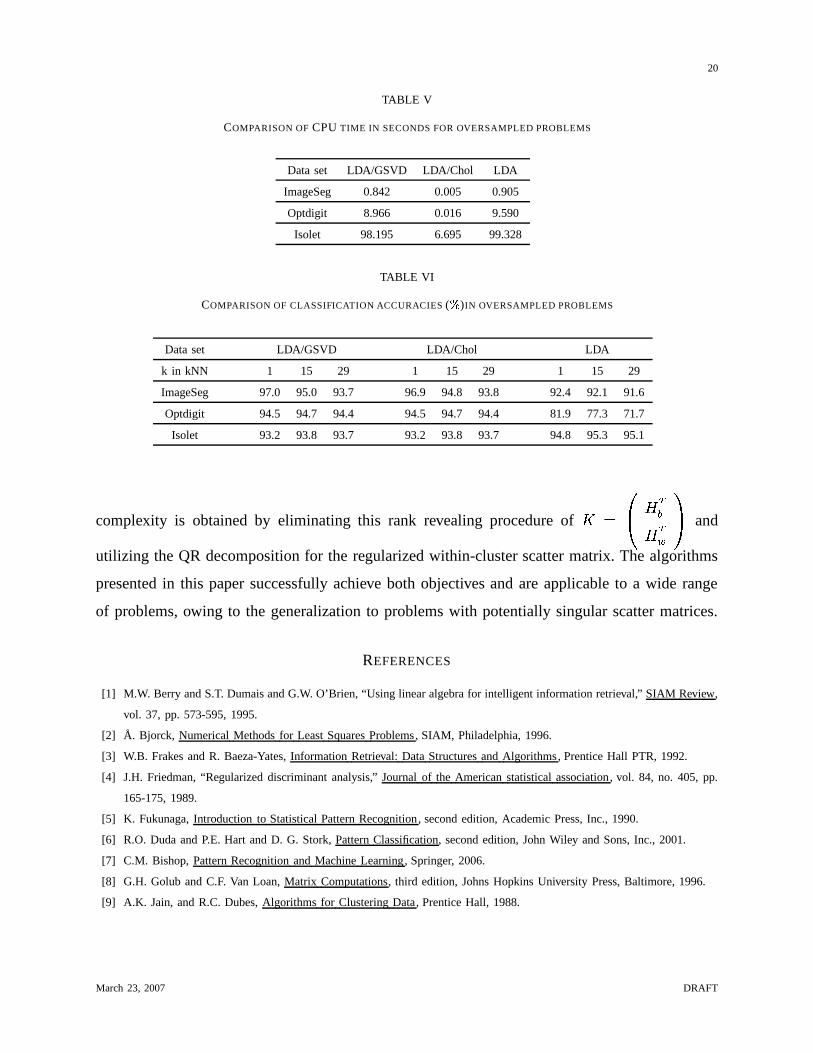
20

TABLE V

COMPARISON OF CPU TIME IN SECONDS FOR OVERSAMPLED PROBLEMS

Data set LDA/GSVD LDA/Chol LDA

ImageSeg 0.842 0.005 0.905

Optdigit 8.966 0.016 9.590

Isolet 98.195 6.695 99.328

TABLE VI

COMPARISON OF CLASSIFICATION ACCURACIES ( � )IN OVERSAMPLED PROBLEMS

Data set LDA/GSVD LDA/Chol LDA

k in kNN 1 15 29 1 15 29 1 15 29

ImageSeg 97.0 95.0 93.7 96.9 94.8 93.8 92.4 92.1 91.6

Optdigit 94.5 94.7 94.4 94.5 94.7 94.4 81.9 77.3 71.7

Isolet 93.2 93.8 93.7 93.2 93.8 93.7 94.8 95.3 95.1

complexity is obtained by eliminating this rank revealing procedure of � #��

��

�� and

utilizing the QR decomposition for the regularized within-cluster scatter matrix. The algorithms

presented in this paper successfully achieve both objectives and are applicable to a wide range

of problems, owing to the generalization to problems with potentially singular scatter matrices.

REFERENCES

[1] M.W. Berry and S.T. Dumais and G.W. O’Brien, “Using linear algebra for intelligent information retrieval,” SIAM Review,

vol. 37, pp. 573-595, 1995.

[2] Å. Bjorck, Numerical Methods for Least Squares Problems, SIAM, Philadelphia, 1996.

[3] W.B. Frakes and R. Baeza-Yates, Information Retrieval: Data Structures and Algorithms, Prentice Hall PTR, 1992.

[4] J.H. Friedman, “Regularized discriminant analysis,” Journal of the American statistical association, vol. 84, no. 405, pp.

165-175, 1989.

[5] K. Fukunaga, Introduction to Statistical Pattern Recognition, second edition, Academic Press, Inc., 1990.

[6] R.O. Duda and P.E. Hart and D. G. Stork, Pattern Classification, second edition, John Wiley and Sons, Inc., 2001.

[7] C.M. Bishop, Pattern Recognition and Machine Learning, Springer, 2006.

[8] G.H. Golub and C.F. Van Loan, Matrix Computations, third edition, Johns Hopkins University Press, Baltimore, 1996.

[9] A.K. Jain, and R.C. Dubes, Algorithms for Clustering Data, Prentice Hall, 1988.


21

[10] P. Howland and M. Jeon and H. Park, “Structure preserving dimension reduction for clustered text data based on the

generalized singular value decomposition,” SIAM Journal on Matrix Analysis and Applications, vol. 25, no. 1, pp. 165-

179, 2003.

[11] P. Howland and H. Park, “Equivalence of several two-stage methods for linear discriminant analysis,” Proc. fourth SIAM

International Conference on Data Mining, Kissimmee, FL, pp. 69-77, April, 2004.

[12] P. Howland and H. Park, “Generalizing Discriminant Analysis Using the Generalized Singular Value Decomposition,”

IEEE Transactions on Pattern Analysis and Machine Intelligence, vol. 26, no. 8, pp. 995-1006, 2004.

[13] G. Kowalski, Information Retrieval Systems: Theory and Implementation, Kluwer Academic Publishers, 1997.

[14] C.L. Lawson and R.J. Hanson, Solving Least Squares Problems, SIAM, Philadelphia, 1995.

[15] C.C. Paige and M.A. Saunders, “Towards a generalized singular value decomposition,” SIAM J. Numer. Anal., vol. 18,

pp. 398-405, 1981.

[16] C. Park and H. Park and P. Pardalos, “A Comparative Study of Linear and Nonlinear Feature Extraction Methods,” Proc.

of 4th ICDM, pp. 495-498, 2004.

[17] C. Park and H. Park, “A relationship between LDA and the generalized minimum squared error solution,” SIAM Journal

on Matrix Analysis and Applications, vol. 27, no. 2, pp. 474-492, 2005.

[18] H. Park and M. Jeon and J.B. Rosen, “Lower dimensional representation of text data based on centroids and least squares,”

BIT, vol. 43, no. 2, pp. 1-22, 2003.

[19] G. Salton, The SMART Retrieval System, Prentice Hall, 1971.

[20] G. Salton and M.J. McGill, Introduction to Modern Information Retrieval, McGraw-Hill, 1983.

[21] S. Theodoridis and K. Koutroumbas, Pattern Recognition, Academic Press, 1999.

[22] C.F. Van Loan, “Generalizing the singular value decomposition,” SIAM J. Numer. Anal., vol. 13, pp. 76-83, 1976.

[23] J. M. Speiser and C.F. Van Loan, “Signal processing computations using the generalized singular value decomposition,”

Proc. SPIE Vol.495, Real Time Signal Processing VII, pp. 47-55, 1984.

[24] C.F. Van Loan and J. M. Speiser, “Computation of the CS Decomposition with Applications to Signal Processing,” Proc.

SPIE Vol.696, Advanced Signal Processing Algorithms and Architectures, 1986.


fast linear discriminant analysis using qr decomposition ...hpark/papers/reglda_ieee.pdf1 fast...

Documents