Fast Nearest-Neighbor Query Processing

in Moving-Object Databases

K. Raptopoulou, Y. Manolopoulos, A.N. PapadopoulosDeptartment of Informatics, Aristotle UniversityThessaloniki 54006, Hellas (Greece){katerina,yannis,apostol}@delab.csd.auth.gr

Abstract. A desirable feature in spatio-temporal databases is the ability to an-swer future queries, based on the current data characteristics (reference positionand velocity vector). Given a moving query and a set of moving objects, a futurequery asks for the set of objects that satisfy the query in a given time interval.The difficulty in such a case is that both the query and the data objects changepositions continuously, and therefore we can not rely on a given fixed referenceposition to determine the answer. Existing techniques are either based on sampling,or on repetitive application of time-parameterized queries in order to provide theanswer. In this paper we develop an efficient method in order to process nearest-neighbor queries in moving-object databases. The basic advantage of the proposedapproach is that only one query is issued per time interval. The Time-ParameterizedR-tree structure is used to index the moving objects. An extensive performanceevaluation, based on CPU and I/O time, shows that significant improvements areachieved compared to existing techniques.

Keywords: spatio-temporal databases, moving objects, nearest-neighbors, continu-ous queries

1. Introduction

Spatio-temporal database systems aim at combining the spatial andtemporal characteristics of data. There are many applications that ben-efit from efficient processing of spatio-temporal queries such as: mobilecommunication systems, traffic control systems (e.g., air-traffic mon-itoring), geographical information systems, multimedia applications.The common basis of the above applications is the requirement tohandle both the space and time characteristics of the underlying data(Sistla, 1997; Wolfson, 1998; Theodoridis, 1998). These applicationspose high requirements concerning the data and the operations thatneed to be supported, and therefore new techniques and tools areneeded towards increased processing efficiency.

Many research efforts have focused on indexing schemes and effi-cient processing techniques for moving-object datasets (Theodoridis,1996; Kollios, 1999b; Agarwal, 2000; Saltenis, 2000; Song, 2001b; Had-jieleftheriou, 2002). A moving dataset is composed of objects whose

c© 2003 Kluwer Academic Publishers. Printed in the Netherlands.

cnn.tex; 5/02/2003; 12:40; p.1

2

positions change with respect to time (e.g., moving vehicles). Examplesof basic queries that could be posed to such a dataset include:

− window query: given a rectangle R that changes position andsize with respect to time, determine the objects that are coveredby R from time point ts to te.

− nearest-neighbor query: given a moving point P determine thek nearest-neighbors of P within the time interval [ts, te].

− join query: given two moving datasets S1 and S2, determine thepairs of objects (s1, s2) with s1 ∈ S1 and s2 ∈ S2 such that s1 ands2 overlap at some point in [ts, te]

Queries that require an answer for a specific time point (time-slicequeries) are special cases of the above examples, and generally are moreeasily processed. Queries that must be evaluated for a time interval[ts, te] are characterized as continuous (Song, 2001a; Tao, 2002a). Insome cases, the query must be evaluated continuously as time advances.The basic characteristic of continuous queries is that there is a changein the answer at specific time points, which must be identified in orderto produce correct results.

Among the plethora of spatio-temporal queries we focus on k nearest-neighbors queries (NN for short). Existing methods are either compu-tationally intensive performing repetitive queries to the database, orare restrictive with respect to the application settings (i.e., are appliedonly for static datasets, or are applicable for special cases that limit thespace dimensionality or the requested number of NNs). The objectiveof this work is twofold:

− to study efficient algorithms for NN query processing on movingobject datasets,

− to compare the proposed algorithms with existing methods throughan extensive experimental evaluation, by considering several pa-rameters that affect query processing performance.

The rest of the article is organized as follows: In the next sectionwe give the appropriate background and related work to keep the pa-per self-contained. In Section 3, the proposed approach is studied indetail and the application to TPR-trees is presented. In Section 4, aperformance evaluation of all methods is conducted and the results areinterpreted. Finally, Section 5 concludes and provides ideas for futurework in the area.

cnn.tex; 5/02/2003; 12:40; p.2

3

2. Background

2.1. Organizing moving objects

The research conducted in access methods and query processing tech-niques for moving-object databases are generally categorized in thefollowing areas:

− query processing techniques for past positions of objects, wherepast positions of moving objects are archived and queried, usingmulti-version access methods or specialized access methods forobject trajectories (Lomet, 1989; Xu, 1990; Kumar, 1998; Nasci-mento, 1998; Pfoser, 2000; Tao, 2001a; Tao, 2001b),

− query processing techniques for present and future positions ofobjects, where each moving object is represented as a function oftime, giving the ability to determine its future positions accordingto the current characteristics of the object movement (referenceposition, velocity vector) (Kollios, 1999a; Kollios, 1999b; Agarwal,2000; Wolfson, 2000; Moreira, 2000; Saltenis, 2000; Procopiuc,2002; Ishikawa, 2002; Kalashnikov, 2002; Lazaridis, 2002).

We focus on the second category, where it is assumed that thedataset consists of moving point objects, which are organized by meansof a Time-Parameterized R-tree (TPR-tree) (Saltenis, 2000). The TPR-tree is an extension of the well known R∗-tree (Beckmann, 1990),designed to handle object movement. Objects are organized in sucha way that a set of moving objects is bounded by a moving rectan-gle, in order to maintain a hierarchical organization of the underlyingdataset. The TPR-tree differs from the R-tree (Guttman, 1984) and itsvariations in several aspects:

− bounding rectangles in the TPR-tree internal nodes although areconservative, they are not minimum in general,

− the TPR-tree is efficient for a time interval [t0,H), where H (hori-zon) is the time point which suggests a reorganization, due toextensive overlapping of bounding rectangles.

− all metrics used for insertion, reinsertion and node splitting inTPR-trees are based on integrals which calculate overlap, enlarge-ment and margin for the time interval [t0, H),

− TPR-trees answer time-parameterized queries (range, NN, joins)for a given time interval [ts, te], or for a specific time point.

cnn.tex; 5/02/2003; 12:40; p.3

4

2.2. Nearest-neighbor queries

Allowing the query and the objects to move, an NN query takes thefollowing forms:

− Given a query point reference position qpos, a query velocity vectorqv, a time point tx and an integer k, determine the k NNs of q attx (time-slice NN query).

− Given a query point reference position q, a query velocity vectorqv, an integer k and a time interval [t1, t2), determine the k NNsof q according to the movement of the query and the movement ofthe objects from t1 to t2 (continuous or time-interval NN query).

The second query type is more difficult to answer, since it requiresknowledge of specific time points which indicate that there is a changein the answer set (split points).

��� ����������

��� ����������

� � � � � � � � � � ���

�

�

�

�

Figure 1. A query example

Figure 1 shows an example database of four moving objects. Assumethat the k = 2 NNs are requested for the time interval [0, 5]. Assumealso that the query point is static (black circle). By observing themovement of the objects with respect to the query, it is evident that forthe time interval [0, 2) the NNs of q are b and a, whereas for the timeinterval [2, 5) the NNs are c and d. In the sequel we briefly describeresearch results towards solving NN queries in moving datasets.

Kollios et al. (Kollios, 1999a) propose a method able to answer NNqueries for moving objects in 1D space. The method is based on the dualtransformation where a line segment in the native space correspondsto a point in the transformed space, and vice-versa. The method de-termines the object that comes closer to the query between [ts, te] andnot the NNs for every time instance.

Zheng et al. (Zheng, 2001) proposed a method for computing a singleNN (k = 1) of a moving query, applied to static points indexed by

cnn.tex; 5/02/2003; 12:40; p.4

5

an R-tree. The method is based on Voronoi diagrams and it seemsquite difficult to be extended for other values of k and higher spacedimensions.

In (Song, 2001a) a method is presented to answer such queries onmoving-query, static-objects cases. Objects are indexed by an R-tree,and sampling is used to query the R-tree at specific points. However,due to the nature of sampling, the method may return incorrect resultsif a split point is missed. A low sampling rate yields more efficientperformance, but increases the probability of incorrect results, whereasa high sampling rate poses unnecessary computational overhead, butdecreases the probability of incorrect results.

Benetis et al. (Benetis, 2002) propose an algorithm capable of an-swering NN queries and reverse NN queries in moving-object datasets.The proposed method is restricted in answering only one NN per query.

In (Tao, 2002a) the authors propose an NN query processing al-gorithm for moving-query moving-objects, based on the concept oftime-parameterized queries. Each query result is composed of the fol-lowing components: i) R, is the current result set of the query, ii) T , isthe time point in which the result becomes invalid, and iii) C, the set ofobjects that influence the result at time T . Therefore, by continuouslycalculating the next set of objects that will influence the result, wedetermine the NNs of the query from t1 to t2. A TPR-tree index isused to organize the moving objects.

The main drawback of the aforementioned method is that the TPR-tree is searched several times in order to determine the next object thatinfluences the current result. This implies additional overhead in CPUand I/O time, which is more severe as the number of requested NNsincreases. In (Tao, 2002b) the same authors present a method whichis applicable for static datasets, in order to overcome the problems ofrepetitive NN queries. By assuming that the dataset is indexed by anR-tree structure, a single query is performed and therefore each partici-pating tree node is accessed only once. Performance results demonstratethat NN queries are answered much more efficiently concerning queryresponse time. However, the proposed techniques can only be appliedfor static datasets.

Table I presents a categorization of NN queries with respect tothe characteristics of queries and datasets. There are four differentversions of the problem which are formulated by considering queriesand datasets as static or moving. The table also summarizes thepreviously mentioned related work for each problem.

cnn.tex; 5/02/2003; 12:40; p.5

6

Table I. NN queries for different query and data charac-teristics.

Query Data Related Work

Static Static conventional techniques

Static Moving handled by MQMD

Moving Static Roussopoulos et al (Song, 2001a)

Zheng et al. (Zheng, 2001)

Tao et al. (Tao, 2002b)

Moving Moving Tao et al. (Tao, 2002a)

Kollios et at. (Kollios, 1999a)

Benetis et al. (Benetis, 2002)

2.3. Motivation

To the best of the authors knowledge, there is no method based onthe TPR-tree to answer NN queries for moving-query moving-objectsother than the repetitive approach proposed in (Tao, 2002a). Therefore,motivated by the extensive overhead of the existing method and takinginto account that the continuous algorithm reported in (Tao, 2002b)can not handle moving-object datasets, we provide efficient methodsfor NN query processing for moving-query moving-object databases,with the following characteristics:

− the method is applied for any number of requested NNs,

− the method can be applied for any number of space dimensions,since only relative distances are computed during query processing,

− different tree pruning algorithms may be applied during tree traver-sal,

− each tree node is accessed only once, therefore reducing the con-sumption of system resources,

− the method not only reports the time points when there is a changein the result, but also the time points when there is a change inthe order of the NNs in the current result.

cnn.tex; 5/02/2003; 12:40; p.6

7

3. NN Query Processing

The challenge is to determine the k NNs of q, given a moving queryq, a query velocity vector vq and a time interval [ts, te]. We want toanswer such a query, by performing only one search, thus avoidingposing repetitive queries to the database. The answer to the query isa set of mutually exclusive time intervals, and a sorted list of objectIDs for each time interval, which are the k NNs of q for the respectiveinterval.

By assuming that the distance between two points is given by theEuclidean distance, the distance Dq,o(t) between query q and object oas a function of time is given by the following equation:

Dq,o(t) =√

c1 · t2 + c2 · t + c3 (1)

where c1, c2, c3 are constants given by:

c1 = (vox − vqx)2 + (voy − vqy)2

c2 = 2 · [(ox − qx) · (vox − vqx) + (oy − qy) · (voy − vqy)]c3 = (ox − qx)2 + (oy − qy)2

vox, voy are the velocities of object o, vqx, vqy are the velocities ofthe query in each dimension, and (ox,oy), (qx, qy) are the referencepositions of the object o and the query q respectively. In the sequel,we assume that the distance is given by (Dq,o(t))2 in order to performsimpler calculations.

The movement of an object with respect to the query is visualizedby plotting the function (Dq,o(t))2, as it is illustrated in Figure 2. ForNN query processing the distance from the query point contains allthe necessary information, since the exact position of the object isirrelevant. Note that since c1 ≥ 0 the plot of the function always hasthe shape of a “valley’.

�

���

� � � � � � � ���

�

Figure 2. Visualization of the distance between a moving object and a moving query

cnn.tex; 5/02/2003; 12:40; p.7

8

(a) k = 2

(b) k = 3

Figure 3. Relative distance of objects with respect to a moving query

Assume that we have a set of moving objects O and a moving queryq. The objects and the query are represented as points in a multi-dimensional space. Although the proposed method can be applied toany number of dimensions, the presentation is restricted to 2D space forclarity and convenience. Moving queries and objects are characterizedby their reference positions and velocity vectors. Therefore, we haveall the necessary information to define the distance (Dq,o(t))2 for everyobject o ∈ O. By visualizing the relative movement of the objectsduring [ts, te] a graphical representation is derived, such as the onedepicted in Figure 3.

By inspecting Figure 3 we obtain the k NNs of the moving queryduring the time interval [ts, te]. For example, for k = 2 the NNs of q forthe time interval are contained in the shaded area of Figure 3. The NNsof q for various values of k along with the corresponding time intervalsare depicted in Figure 4. The pair of objects above each time point txdeclare the objects that have an intersection at tx. These time points

cnn.tex; 5/02/2003; 12:40; p.8

9

where a modification of the result is performed, are called split points.Note that not all intersection points are split points. For example, theintersection of objects a and c in Figure 3 is not considered as a splitpoint for k = 2 , whereas it is a split point for k = 3.

��� ��� ��� ��� �� ��

� � � �

� � � � � � � � � ��� �� �

� � � � � �

Figure 4. NNs of the moving query for k = 2 (top) and k = 3 (bottom)

The previous example demonstrates that the k NNs of a movingquery can be determined by using the functions that represent thedistance of each moving object with respect to the moving query. Basedon the previous discussion, the next section presents the design of analgorithm for NN query processing (NNS) which operates on movingobjects.

3.1. The NNS Algorithm

The NNS algorithm consists of two parts, which are described sepa-rately:

− NNS-a algorithm: given a set of moving objects, a moving queryand a time interval, the algorithm returns the k NNs for the giveninterval, and

− NNS-b algorithm: given the k NNs, the corresponding time inter-vals, and a new moving object, the algorithm computes the newresult.

3.1.1. Algorithm NNS-aWe are given a moving query q, a set O of N moving objects, a timeinterval [ts, te] and the k NNs of q are requested. The target is topartition the time interval into one or more sub-intervals, in whichthe list of NNs remains unchanged. Each time sub-interval is definedby two time split points, declaring the beginning and the end of thesub-interval. During the calculation, the set O is partitioned into threesub-sets:

cnn.tex; 5/02/2003; 12:40; p.9

10

− the set K, which always contains k objects that are currently theNNs of q,

− the set C, which contain objects that are possible candidates forsubsequent time points, and

− the set R, which contains rejected objects whose contribution tothe answer is impossible for the given time interval [ts, te].

Initially, K = ∅, C = O, and R = ∅. The first step is to determinethe k NNs for time point ts. By inspecting Figure 3 for k = 2 we getthat these objects are a and b. Therefore, K={a, b}, C={c, d, e} andR=∅. Next, for each o ∈ K the intersections with objects in K + Care determined. If there are any objects in C that do not intersect anyobjects in K, they are removed from C and are put in R, meaningthat they will not be considered again (Proposition 1). In our example,object e is removed from C and we have K={a, b}, C={c, d} andR={e}.The currently determined intersections are kept in an ordered list, inincreasing time order. Each intersection is represented as (tx, {u, v}),where tx is the time point of the intersection and {u, v} is the objectsthat intersect at tx.

PROPOSITION 1. Moving objects that do not intersect the k nearestneighbors of the query at time ts, can be rejected.

ProofAn intersection between o1 and o2 denotes a change in the result. There-fore, if none of the k nearest-neighbor objects intersect any other objectbetween [ts, te], there will be no change in the result. This means thatwe do not have to consider other objects for determining the nearest-neighbors. 2

Each intersection is defined by two objects 1 u and v. The cur-rently determined intersection points comprise the current list of timesplit points. According to the example, the split point list has as fol-lows: (t1, {a, b}), (t2, {a, d}), (tx, {a, c}), (t3, {b, d}), (t4, {b, c}). For eachintersection we distinguish between two cases:

− u ∈ K and v ∈ K− u ∈ K and v ∈ C (or u ∈ C and v ∈ K)

1 It is assumed that an intersection is defined by two objects. If three or moreobjects intersect at the same point tx the conflict is resolved by evaluating the firstderivative for each object at tx and taking the minimum value.

cnn.tex; 5/02/2003; 12:40; p.10

11

In the first case, the current set of NNs does not change. However, theorder of the currently determined objects changes, since two objects inK intersect, and therefore they exchange their position in the orderedlist of NNs. Therefore, objects u and v exchange their position. In thesecond case, object v is inserted into K and therefore the list of NNsmust be updated accordingly (Proposition 2).

PROPOSITION 2. Let us consider a split point at time tx, at whichobjects o1 and o2 intersect. If o1 ∈ K and o2 ∈ C then at tx, o1 is thek-th nearest-neighbor of the query.

ProofAssume that o1 is not the k-th nearest-neighbor at the time of theinterscection. However, o1 belongs to the result (is among the k nearest-neighbors) at time tx. The intersection at time tx denotes that objectso1 and o2 are consequtive in the result. This implies that o2 is alreadycontained in the current result (set K) which contradicts our assump-tion that o2 is not contained in the result set. Therefore, object o1 mustbe the k-th nearest-neighbor of the query. 2

According to the currently determined split points, the first splitpoint is t1, where objects a and b intersect. Since both objects arecontained in K, no new objects are inserted into K, and simply objectsa and b exchange their position. Up to this point concerning the sub-interval [ts, t1) the nearest neighbors of q are a and b. We are readynow to check the next split point, which is t2 where objects a and dintersect. Since a ∈ K and d ∈ C object a is removed from K and it isinserted into C. On the other hand, object d is removed from C and it isinserted into K taking the position of a. Up to this point, another partof the answer has been determined, since in the sub-interval [t1, t2) theNNs of q are b and a. Moving to the next intersection, tx, we see thatthis intersection is caused by objects a and c. However, neither of theseobjects is contained in K. Therefore, we ignore tx and remove it fromthe list of time split points. Since a new object d has been inserted intoK, we check for new intersections between d and objects in K and C.No new intersections are discovered, and therefore we move to the nextsplit point t3. Currently, for the time sub-interval [t2, t3) the NNs of qare b and d. At t3 objects b and d intersect, and this causes a positionexchange. We move to the next split point t4 where objects b and cintersect. Therefore, object b is removed from K and it is inserted intoC, whereas object c is removed from C and it is inserted into K. Sincec does not have any other intersections with objects in K and C, thealgorithm terminates. The final result is depicted in Figure 4, along

cnn.tex; 5/02/2003; 12:40; p.11

12

with the corresponding result for k = 3. The outline of the method isillustrated in Figure 5.

Algorithm NNS-aInput: a set of moving objects O, a moving query q,time interval [ts, te], the number k of requested NNsOutput: a list of elements of the form ([t1, t2], o1, o2, ..., ok)where o1, ..., ok are the NNs of q from t1 to t2 (CNN-list),split-list containing the split pointsLocal: k-list containing the current NNs1. initialize K = ∅, C = O, and R = ∅2. initialize split-list with split points ts and te3. find the k NNs of q at time point ts4. update k-list5. foreach u ∈ K do6. find intersections with v ∈ K7. find intersections with v ∈ C8. update split list9. move irrelevant objects from C to R10. endfor11. while more split-points are available do12. check next time split point tx (intersection)13. if (u ∈ K) and (v ∈ K) then14. update CNN-list15. exchange positions in k-list16. endif17. if (u ∈ K) and (v ∈ C) then18. move u from K to C19. move v from C to K20. update k-list21. update CNN-list22. if (v participates for the first time in k-list) then23. determine intersections of v with objects in C24. update split-list25. endif26. endif27. if (u ∈ C) and (v ∈ C) then28. ignore split point tx29. endif30. endwhile31. return CNN-list, split-list

Figure 5. The NNS-a algorithm

Each object o ∈ K is responsible for a number of potential timesplit points, which are defined by the intersections of o and the objectscontained in C. Therefore, each time an object is inserted into K in-tersection checks must be performed with the objects in C. In orderto reduce the number of intersection tests, if an object was previouslyinserted into K and now it is reinserted, it is not necessary to recomputethe intersections. Moreover, according to Proposition 3, intersections at

cnn.tex; 5/02/2003; 12:40; p.12

13

time points prior to the currently examined split point can be safelyignored.

PROPOSITION 3. If there is a split point at time tx, where o1 ∈ Kand o2 ∈ C intersect, all intersections of o2 with the other objects in Kthat occur at a time before tx are not considered as split points.

ProofThis is evident, since the nearest-neighbors of the query object up totime tx have been already determined and therefore the intersectionsat time points prior to tx do not denote a change in the result. 2

Evidently, in order to determine if two objects u and v intersectat some time point between ts and te, we have to solve an equation.Let the square of the Euclidean distance between q and the objects bedescribed by the functions Du,q(t)2 = u1 · t2 +u2 · t+u3 and Dv,q(t)2 =v1 · t2 + v2 · t + v3 respectively. In order for the two object to have anintersection in [ts, te] there must be at least one value tx, ts ≤ tx ≤ tesuch that:

(u1 − v1) · t2x + (u2 − v2) · tx + (u3 − v3) = 0

From elementary calculus it is known that this equation can be satisfiedby none, one, or two values of tx. If (u2−v2)2−4·(u1−v1)·(u3−v3) < 0,then there is no intersection between u and v. If (u2 − v2)2 − 4 · (u1 −v1) · (u3 − v3) = 0 then the two objects intersect at tx = −(u2−v2)

2·(u1−v1) .Otherwise the objects intersect at two points tx and ty given by:

tx =−(u2 − v2) +

√(u2 − v2)2 − 4 · (u1 − v1) · (u3 − v3)

2 · (u1 − v1)

ty =−(u2 − v2)−

√(u2 − v2)2 − 4 · (u1 − v1) · (u3 − v3)

2 · (u1 − v1)

3.1.2. Algorithm NNS-bAfter the execution of NNS-a, the CNN-list is formulated, which con-tains elements of the form: ([t1, t2], o1, o2, ..., ok) where o1, ..., ok are theNNs of q from t1 to t2, in increasing distance order. Let S be the setcontaining the NNs of q at any given time between ts and te. Clearly,k ≤ |S| ≤ |O|. Assume now that we have to consider another object w,which was not known during the execution of NNS-a. We distinguishamong the following cases, which describe the relation of w to thecurrent answer:

cnn.tex; 5/02/2003; 12:40; p.13

14

case 1: w does not intersect any of the objects in S between ts and te,and it is “above” the area of relevance. In this case, w is ignored,since it can not contribute to the NNs. The number of split pointsremains the same.

case 2: w does not intersect any of the objects in S between ts andte, and it is completely “inside” the area of relevance. In this casew must be taken into account, since it affects the answer from tsto te (Proposition 4). The number of split points may be reduced.

case 3: w intersects at least one object v ∈ S at time ts ≤ tx ≤ te,but at time tx v is not contained in the set of NNs. In this case,again w is ignored, since this intersection can not be considered asa split point because the answer is not affected. Therefore, no newsplit points are generated.

case 4: w intersects at least one object v ∈ S at time ts ≤ tx ≤ te,and object v is contained in the set of NNs at time tx. In thiscase w must be considered because at least one new split pointis generated. We note, however, that some of the old split pointsmay be discarded.

PROPOSITION 4. Assume that a new object w does not intersect anyof the NNs from ts to te. If at time ts its position among the k NNs isposw, then it maintains this position throughout the query duration.

ProofAssume that there is a change in the result at some point tx, whereobject w changes its position among the nearest-neighbors. This im-plies that there is an intersection at time tx, since only an intersectiondenotes a result change. This contradicts our assumption that there areno intersections of w with other objects in the result. 2

The aforementioned cases are depicted in Figure 6. Object e cor-responds to case 1, since it is above the area of interest. Object fcorresponds to case 2, because it is completely covered by the rele-vant area. Object g although intersects some objects, the time of theseintersections are irrelevant to the answer, and therefore the situationcorresponds to case 3. Finally, object h intersects a number of objectsat time points that are critical to the answer and therefore correspondsto case 4.

The outline of the NNS-b algorithm is presented in Figure 7. Notethat in lines 14 and 20 a call to the procedure modify-CNN-list isperformed. This procedure, takes into consideration the CNN-list and

cnn.tex; 5/02/2003; 12:40; p.14

15

Figure 6. The four different cases that show the relation of a new object to thecurrent NNs

Algorithm NNS-bInput: a list of elements of the form ([t1, t2], o1, o2, ..., ok)where o1, ..., ok are the NNs of q from t1 to t2 (CNN list),a new object w, the split-listOutput: an updated list of the form ([t1, t2], o1, o2, ..., ok)where o1, ..., ok are the NNs of q from t1 to t2 (CNN list)Local: k-list current list of NNs,split-list, the current list of split points1. initialize S = union of NNs from ts to te2. intersectionFlag = FALSE3. foreach s ∈ S do4. check intersection between s and w5. if (s and w intersect) then // handle cases 3 and 46. intersectionFlag = TRUE7. collect all tj , s // tj is where w and s intersect8. if (at tj object s contributes to the NNs) then9. update split-list10. endif11. endif12. endfor13. if (intersectionFlag == TRUE) then14. call modify-CNN-list15. else // handle cases 1 and 216. calculate Dq,w(t)2 at time point ts17. if (Dq,w(ts)2 ≥ D2

kNN ) then18. ignore w19. else20. call modify-CNN-list21. endif22. endif23. return CNN-list, split-list

Figure 7. The NNS-b algorithm

the new split-list that is generated. It scans the split-list in increasingtime order and performs the necessary modifications to the CNN-list

cnn.tex; 5/02/2003; 12:40; p.15

16

and the split-list. Some of the split-points may be discarded during theprocess. The steps of the procedure are illustrated in Figure 8.

Procedure modify-CNN-listInput: a list of elements ([t1, t2], o1, o2, ..., ok)where o1, ..., ok are the NNs of q from t1 to t2 (CNN list),a new object w, the split-listOutput: an updated list of elements ([t1, t2], o1, o2, ..., ok)where o1, ..., ok are the NNs of q from t1 to t2 (CNN list)Local: k-list current list of NNs1. calculate Dq,w(t)2 at time point ts2. consult CNN-list and update the current k-list3. while more split-points are available do4. check next split-point (tx, {u, v})5. update CNN-list6. if (u /∈ k − list) and (v /∈ k − list) then7. remove split-point (tx, {u, v})8. elseif (u ∈ k − list) and (v /∈ k − list) then9. remove u from k-list10. insert v in k-list11. update k-list12. elseif (v ∈ k − list) and (u /∈ k − list) then13. remove v from k-list14. insert u in k-list15. update k-list16. else17. exchange positions between u and v18. update k-list19. endif20. endwhile

Figure 8. The modify-CNN-list procedure

3.2. Query Processing with TPR-trees

Having described in detail the query processing algorithms in the pre-vious section we are ready now to elaborate in the way these methodsare combined with the TPR-tree. Let T be a TPR-tree which is builtto index the underlying data. Starting from the root node of T the treeis searched in a depth-first-search manner (DFS) 2. The first phase ofthe algorithm is completed when m ≥ k objects have been collectedfrom the dataset. Tree branches are selected for descendant accordingto the mindist metric (Roussopoulos, 1995) (Definition 1) between themoving query and bounding rectangles at time ts. These m movingobjects are used as input to the NNS-a algorithm in order to determinethe result from ts to te. Therefore, up to now we have a first version

2 The proposed methods can also be combined with a breadth-first-search basedalgorithm.

cnn.tex; 5/02/2003; 12:40; p.16

17

of the split-list and the CNN-list. However, other relevant objects mayreside in leaf nodes of T that are not yet examined.

DEFINITION 1. Given a point p at (p1, p2, ...,pn and a rectangle rwhose lower-left and upper-right corners are (s1, s2 , ..., sn) and (t1, t2, ...,tn),the distance mindist(p, r) is defined as follows:

mindist(p, r) =

√√√√n∑

j=1

|pj − rj |2

where:

rj =

sj , pj < sj

tj , pj > tjpj , otherwise

2

In the second phase of the algorithm, the DFS continues to searchthe tree, by selecting possibly relevant tree branches and dis-carding non-relevant ones. Every time a possibly relevant movingobject is reached, algorithm NNS-b is called in order to update thesplit-list and the CNN-list of the result. The algorithm terminates whenthere are no relevant branches to examine.

In order to complete the description of the algorithm, the termspossibly relevant tree branches and possibly relevant movingobjects must be clarified. In other words, the pruning strategy must bedescribed in detail. Figure 9 illustrates two possible pruning techniquesthat can be used to determine relevant and non-relevant tree branchesand moving objects:

Pruning Technique 1 (PT1): In this technique we keep track of themaximum distance Dmax between the query and the current setof NNs. In Figure 9(a) this distance is defined between the queryand object b at time tstart. We formulate a moving boundingrectangle R centered at q with extends Dmax in each dimensionand moving with the same velocity vector as q. If R intersects abounding rectangle E in an internal node, the corresponding treebranch may contain objects that contribute to the answer andtherefore must be examined further. Otherwise, it can be safelyrejected since it is impossible to contain relevant objects. In thesame manner, if a moving object ox found in a leaf node intersectsR it may contribute to the answer, otherwise it is rejected.

Pruning Technique 2 (PT2): This technique differs from the previ-ous one in the level of granularity that moving bounding rectangles

cnn.tex; 5/02/2003; 12:40; p.17

18

(a) one bounding rectangle

(b) many bounding rectangles

Figure 9. Pruning techniques

are formulated. Instead of using only one bounding rectangle, a setof bounding rectangles is defined according to the currently deter-mined split points. Note that it is not necessary to consider all splitpoints, but only these that are defined by the k-th nearest-neighborin each time interval. An example set of moving bounding rectan-gles is illustrated in Figure 9(b). Each internal bounding rectangleand moving object is checked for intersection with the whole setof moving bounding rectangles and it is considered relevant onlyif it intersects at least one of them.

Other pruning techniques can also be determined by grouping splitpoints in order to keep the balance between the number of generatedbounding rectangles and the existing empty space. Several pruningtechniques can be combined in a single search by selecting the pre-ferred technique according to some criteria (e.g., current number ofsplit-points, existing empty space).

cnn.tex; 5/02/2003; 12:40; p.18

19

It is anticipated that PT1 will be more efficient with respect to CPUtime, but less efficient concerning I/O time, because the empty spacewill cause unnecessary disk accesses. On the other hand, PT2 seems toincur more CPU overhead due to the increased number of intersectioncomputations, but also less I/O time owing to the detailed pruningperformed. Based on the above discussion, we define the NNS-CONalgorithm which operates on TPR-trees and can be used with either ofthe two pruning techniques. The outline of the algorithm is illustratedin In Figure 10.

Algorithm NNS-CONInput: the TPR-tree root,

a moving query q,the number k of NNs

Output: the k NNs in [ts, te]Local: a set O of collected objects,

Flag is FALSE if NNS-a has not yet been callednumber col of collected objects1. if (node is LEAF) then2. if (|O| < k) then3. add each entry of node to O4. update |O|5. endif6. if (|O| ≥ k) and (Flag == FALSE) then7. call NNS-a8. set Flag=TRUE9. elseif (|O| ≥ k) and (Flag == TRUE) then10. apply pruning technique11. for each entry of node call NNS-b12. endif13. elseif (node is INTERNAL) then14. apply pruning technique15. sort entries of node wrt mindist at ts16. call NNS-CON recursively17. endif

Figure 10. The NNS-CON algorithm

4. Performance Evaluation

4.1. Preliminaries

In the sequel a description of the performance evaluation procedureis given, aiming at providing a comparison study among the differ-ent processing methods. The methods under consideration are i) theNNS-CON algorithm enabled by pruning technique 1 described in theprevious section, and ii) the NNS-REP algorithm which operates by

cnn.tex; 5/02/2003; 12:40; p.19

20

posing repetitive NN queries to the TPR-tree (Tao, 2002b). Both algo-rithms as well as the TPR-tree access method have been implementedin the C programming language.

Table II. Parameters and corresponding values

Parameter Value

database size, N 10K, 50K, 100K, 1M

space dimensions, d 1, 2, 3

data distribution, D uniform, gaussian

number of NNs, k 1 - 100

travel time, ttravel 26 - 1048 sec.

LRU buffer size, B 0.1% - 20% of tree pages

There are several parameters that contribute to the method perfor-mance. These parameters, along with their respective values assignedduring the experimentation are summarized in Table II.

The datasets used for the experimentation are synthetically gener-ated using the uniform or the gauss distribution. The dataspace extendsare 1,000,000 x 1,000,000 meters and the velocity vectors of the movingobjects are uniformly generated, having speed values between 0 and 30m/sec. Based on these objects, a TPR-tree is constructed. The pagesize of the TPR-tree is fixed at 2Kbytes.

The query workload is composed of 500 uniformly distributed querieshaving the same characteristics (length, velocity). The comparison studyis performed by using several performance indices, such as: i) the num-ber of disk accesses, ii) the CPU-time, iii) the I/O time and iv) the totalrunning time. In order to accurately estimate the I/O time for eachmethod a disk model is used to model the disk, instead of assigning aconstant value for each disk access (Ruemmler, 1994). Since the usageof a buffer plays a very important role for the query performance weassume the existence of an LRU buffer having its size vary between0.1% and 20% of the database size.

The results presented here correspond to uniformly distributed datasets.Results performed for gaussian distributions of data and queries demon-strated similar performance and therefore are omitted. The main dif-ference between the two distributions is that in the case of the gaus-sian distribution, the algorithms require more resources since the data

cnn.tex; 5/02/2003; 12:40; p.20

21

density increases and therefore more split-points and distance compu-tations are needed to evaluate the queries.

4.2. Performance Results

Several experimental series have been conducted in order to test theperformance of the different methods. The experimental series are sum-marized in Table III.

Table III. Experiments conducted

Experiment Varying Parameter Fixed Parameters

N = 1M ,

EXP1 NNs, k B = 10%,

ttravel = 110 sec.

d = 2, D=uniform

N = 1M ,

EXP2 buffer size, B k = 5,

ttravel = 110 sec.

d = 2, D=uniform

N = 1M ,

EXP3 travel time, ttravel k = 5,

B = 10%,

d = 2, D=uniform

space dimensions, d N = 1M,

EXP4 NNs, k B = 10%,

ttravel = 110 sec.

D=uniform

database size, N B = 500 pages,

EXP5 NNs, k d = 2,

D=uniform,

ttravel = 110 sec.

The purpose of the first experiment (EXP1) is to investigate thebehavior of the methods for various values of the requested NNs. Thecorresponding results are depicted in Figure 11. By increasing k, moresplit points are introduced for the NNS-CON method, whereas moreinfluence calculations are needed by the NNS-REP method. It is evi-dent that NNS-CON outperforms significantly the NNS-REP method.Although both methods are highly affected by k, the performance ofNNS-REP degrades more rapidly. As Figure 11(a) illustrates, NNS-REP requires a large number of node accesses. However, since there is

cnn.tex; 5/02/2003; 12:40; p.21

22

a high locality in the page references performed by a query, the pagefaults are limited. As a result, the performance difference occurs dueto the increased CPU cost required by NNS-REP (Figure 12). Anotherinteresting observation derived from Figure 12 is that the CPU costbecomes more significant than the I/O cost by increasing the numberof nearest-neighbors.

The next experiment (EXP2) illustrates the impact of the buffercapacity (Figure 13). Evidently, the more buffer space is available theless disk accesses are required by both methods. It is interesting thatalthough the number of node accesses required by NNS-REP is verylarge, (see Figure 11(a)) the buffer manages to reduce the number ofdisk accesses significantly due to buffer hits. However, even if the buffercapacity is limited, NNS-CON demonstrates excellent performance.

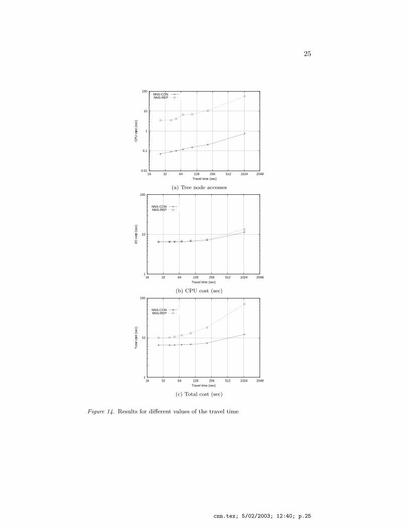
Experiment EXP3 demonstrates the impact of the travel time to theperformance of the methods. The corresponding results are depicted inFigure 14. Small travel times are favorable for both methods, becauseless CPU and I/O operations are required. On the other hand, largetravel times increase the number of split-points and the number of dis-tance computations, since the probability that there is a change in theresult increases. However, NNS-CON performs much better for largetravel times in contrast to NNS-REP whose performance is affectedsignificantly.

The next experiment (EXP4) demonstrates the impact of the spacedimensionality. The increase in the dimensionality has the followingresults: i) the database size increases due to smaller tree fanout, ii)the TPR-tree quality degrades due to overlap increase in boundingrectangles of internal nodes, and iii) the CPU cost increases becausemore computations are required for distance calculations. Both meth-ods are affected by the dimensionality increase. However, by observingthe relative performance of the methods (NNS-REP over NNS-CON) in2D and 3D space illustrated in Figure 15, it is realized that NNS-REPis affected more significantly by the number of space dimensions.

Finally, Figure 16 depicts the impact of database size (EXP5). In thisexperiment, the buffer capacity is fixed to 500 pages, and the numberof moving objects is set between 10,000 and 100,000. The number ofrequested NNs is varying between 1 and 15, whereas the travel time isfixed to 110 sec. By increasing the number of moving objects, more treenodes are generated and, therefore, more time is needed to search theTPR-tree. Moreover, by keeping the buffer capacity constant, the bufferhit ratio decreases, producing more page faults. As Figure 16 illustrates,the performance ratio (NNS-REP over NNS-CON) increases with thedatabase size.

cnn.tex; 5/02/2003; 12:40; p.22

23

1000

10000

100000

1e+06

1 2 4 8 16 32

TP

R n

ode

acce

sses

Number of NNs (k)

NNS-CONNNS-REP

(a) Tree node accesses

0.01

0.1

1

10

100

1 2 4 8 16 32

CP

U c

ost (

sec)

�

Number of NNs (k)

NNS-CONNNS-REP

(b) CPU cost (sec)

1

10

100

1 2 4 8 16 32

Tot

al c

ost (

sec)

�

Number of NNs (k)

NNS-CONNNS-REP

(c) Total cost (sec)

Figure 11. Results for different values of the number of NNs

cnn.tex; 5/02/2003; 12:40; p.23

24

0.01

0.1

1

10

0 2 4 6 8 10 12 14 16 18 20

CP

U c

ost o

ver

I/O c

ost

�

Number of NNs

NNS-CONNNS-REP

Figure 12. CPU cost over I/O cost

1

10

100

1000

0.0625 0.125 0.25 0.5 1 2 4 8 16 32

Tot

al c

ost (

sec)

�

Buffer size (percentage of db size)

NNS-CONNNS-REP

Figure 13. Results for different buffer capacities

cnn.tex; 5/02/2003; 12:40; p.24

25

0.01

0.1

1

10

100

16 32 64 128 256 512 1024 2048

CP

U c

ost (

sec)

�

Travel time (sec)

NNS-CONNNS-REP

(a) Tree node accesses

1

10

100

16 32 64 128 256 512 1024 2048

I/O c

ost (

sec)

�

Travel time (sec)

NNS-CONNNS-REP

(b) CPU cost (sec)

1

10

100

16 32 64 128 256 512 1024 2048

Tot

al c

ost (

sec)

�

Travel time (sec)

NNS-CONNNS-REP

(c) Total cost (sec)

Figure 14. Results for different values of the travel time

cnn.tex; 5/02/2003; 12:40; p.25

26

1

10

100

1 2 3 4 5 6 7 8 9 10

Rel

ativ

e pe

rfor

man

ce

�

Number of NNs (k)

2D space3D space

Figure 15. Results for different space dimensions

1

10

100

0 2 4 6 8 10 12 14 16

Rel

ativ

e pe

rfor

man

ce

�

Number of NNs (k)

10,00050,000

100,000

Figure 16. Results for different database size

cnn.tex; 5/02/2003; 12:40; p.26

27

5. Concluding Remarks

Applications that rely on the combination of spatial and temporalcharacteristics of the objects demand new types of queries and efficientquery processing techniques. An important query type in such a case isthe k nearest-neighbor query, which requires the determination of the kclosest objects to the query for a given time interval [ts, te]. The majordifficulty in such a case is that both queries and objects change positionscontinuously, and therefore the methods that solve the problem for thestatic case can not be applied directly.

In this work, a study of efficient methods for NN query processing inmoving-object databases is performed, and several performance evalu-ation experiments are conducted to compare their efficiency. The mainconclusion is that the proposed algorithm outperforms significantly therepetitive approach for different parameter values. Future research mayfocus on:

− extending the algorithm to work with moving rectangles (althoughthe extension is simple, the complexity of the algorithm increasesdue to more distance computations),

− comparing the performance of different pruning techniques,

− studying the performance of the method to other access methodslike the STAR-tree (Procopiuc, 2002),

− modifying the algorithm to provide the ability for incremental com-putation of the NNs, as the work in (Hjaltason, 1995; Hjaltason,1999) suggests for static datasets,

− adapting the method to operate on access methods which storepast positions of objects (trajectories), in order to answer pastqueries, and

− providing cost estimates concerning the number of node accesses,the number of intersection checks and the number of distancecomputations.

cnn.tex; 5/02/2003; 12:40; p.27

28

References

Agarwal P.K., Arge L. and Erickson J.: “Indexing Moving Points”, ACM PODS,pp.175-186, 2000.

Beckmann N., Kriegel H.P. and Seeger B.: “The R∗-tree: an Efficient and RobustMethod for Points and Rectangles”, ACM SIGMOD, pp.322-331, 1990.

Benetis R., Jensen C.S., Karciauskas G. and Saltenis S.: “Nearest Neighbor andReverse Nearest Neighbor Queries for Moving Objects”, IDEAS, pp.44-53, 2002.

Guttman A.: “R-trees: a Dynamic Index Structure for Spatial Searching”, ACMSIGMOD, pp.47-57, 1984.

Hadjieleftheriou M., Kollios G., Tsotras V.J. and Gunopoulos D.: “Efficient Indexingof Spatio-Temporal Objects”, EDBT, pp.251-268, 2002.

Hjaltason G. and Samet H.: “Ranking in Spatial Databases”, SSD, pp. 83-95, 1995.Hjaltason G. and Samet H.: “Distance Browsing in Spatial Databases”, ACM TODS,

24(2), pp.265-318, 1999.Ishikawa Y. and Kitagawa H. and Kawashima T.: “Continual Neighborhood

Tracking for Moving Objects Using Adaptive Distances”,IDEAS, pp.54-63, 2002.Kalashnikov D.V., Prabhakar S., Hambrusch S.E. and Aref W.G.: “Efficient Eval-

uation of Continuous Range Queries on Moving Objects, DEXA, pp.731-740,2002.

Kollios G., Gounopoulos D. and Tsotras V.J.: “Nearest Neighbor Queries in a MobileEnvironment”, Proceedings of the International Workshop on Spatio-temporalDatabase Management, pp.119-134, 1999.

Kollios G., Gunopoulos D. and Tsotras V.: “On Indexing Mobile Objects”, ACMPODS, pp.261-272, 1999.

Kumar A., Tsotras V.J. and Faloutsos C.: “Designing Access Methods for Bitem-poral Databases”, IEEE TKDE, pp.1-20, 1998.

Lazaridis I., Porkaew I. and Mehrotra S.: “Dynamic Queries over Mobile Objects”,EDBT, pp.269-286, 2002.

Lomet D. and Salsberg B.: “Access Methods for Multiversion Data”, ACMSIGMOD, pp.315-324, 1989.

Moreira J., Ribeiro C. and Abdessalem T.: “Query Operations for Moving ObjectsDatabase Systems”, ACM-GIS, pp.108-114, 2000.

Nascimento M.A. and Silva J.R.O.: “Towards Historical R-trees”, ACM SAC, 1998.Pfoser D., Jensen C.S. and Theodoridis Y.: “Novel Approaches to the Indexing of

Moving Object Trajectories”, VLDB, pp.395-406, 2000.Procopiuc C.M., Agarwal P.K. and Har-Peled S.: “STAR-Tree: An Efficient Self-

Adjusting Index for Moving Objects”, ALENEX, pp.178-193, 2002.Roussopoulos N., Kelley S. and Vincent F.: “Nearest Neighbor Queries”. ACM

SIGMOD, pp. 71-79, 1995.Ruemmler C. and Wilkes J.: “An Introduction to Disk Drive Modeling”, IEEE

Computer, 27(3), pp.17-29, 1994.Saltenis S., Jensen C.S., Leutenegger S. and Lopez M.: “Indexing the Positions of

Continuously Moving Objects”, ACM SIGMOD, pp.331-342, 2000.Sistla A.P., Wolfson O., Chamberlain S. and Dao S.: “Modeling and Querying

Moving Objects”, IEEE ICDE, pp.422-432, 1997.Song Z. and Roussopoulos N.: “K-NN Search for Moving Query Point”, SSTD,

pp.79-96, 2001.Song Z. and Roussopoulos N.: “Hashing Moving Objects”, Mobile Data Manage-

ment, pp.161-172, 2001.Tao Y. and Papadias D.: “Efficient Historical R-trees”, SSDBM, 2001.

cnn.tex; 5/02/2003; 12:40; p.28

29

Tao Y. and Papadias D.: “MV3R-tree - a Spatio-Temporal Access Method forTimestamp and Interval Queries”, VLDB, pp.431- 440, 2001.

Tao Y., Papadias D. and Shen Q.: “Continuous Nearest Neighbor Search”, VLDB,pp.287-298, 2002.

Tao Y. and Papadias D.: “Time-Parameterized Queries in Spatio-TemporalDatabases” ACM SIGMOD, pp. 334-345, 2002.

Theodoridis Y., Vazirgiannis M. and Sellis T.: “Spatio-temporal Indexing for LargeMultimedia Applications”, Proceedings of 3rd IEEE Conference on MultimediaComputing and Systems, pp.441-448, 1996.

Theodoridis Y., Sellis T., Papadopoulos A.N. and Manolopoulos Y.: “Specificationsfor Efficient Indexing in Spatio-Temporal Databases”, SSDBM, pp.123-132, 1998.

Wolfson O., Xu B., Chamberlain S. and Jiang L.: “Moving Objects Databases: Issuesand Solutions”, SSDBM, pp.111-122, 1998.

Wolfson O., Xu B. and Chamberlain S.: “Location Prediction and Queries forTracking Moving Objects”, ICDE, pp.687-688, 2000.

Xu X., Han J. and Lu W.: “RT-tree: an Improved R-tree Index Structure for Spatio-Temporal Databases”, SDH, pp.1040-1049, 1990.

Zheng B. and Lee D.: “Semantic Caching in Location-Dependent Query Processing”,SSTD, pp.97-116, 2001.

cnn.tex; 5/02/2003; 12:40; p.29

cnn.tex; 5/02/2003; 12:40; p.30