Fast probabilistic petrophysical mapping of reservoirsfrom 3D seismic data

Mohammad S. Shahraeeni1, Andrew Curtis2, and Gabriel Chao3

ABSTRACT

A fast probabilistic inversion method for 3D petrophysicalproperty prediction from inverted prestack seismic data has beendeveloped and tested on a real data set. The inversion objective isto estimate the joint probability density function (PDF) of modelvectors consisting of porosity, clay content, and water saturationcomponents at each point in the reservoir, from data vectors withcompressional- and shear-wave-impedance components that areobtained from the inversion of seismic data. The proposed inver-sion method is based on mixture density network (MDN), whichis trained by a given set of training samples, and provides an es-timate of the joint posterior PDF’s of the model parameters forany given data point. This method is much more time and mem-ory efficient than conventional nonlinear inversion methods. Thetraining data set is constructed using nonlinear petrophysical for-ward relations and includes different sources of uncertainty in the

inverse problem such as variations in effective pressure, bulkmodulus and density of hydrocarbon, and random noise in re-corded data. Results showed that the standard deviations of allmodel parameters were reduced after inversion, which shows thatthe inversion process provides information about all parameters.The reduction of uncertainty in water saturation was smaller thanthat for porosity or clay content; nevertheless the maximum of thea posteriori (MAP) of model PDF clearly showed the boundarybetween brine saturated and oil saturated rocks at wellbores. TheMAP estimates of different model parameters show the lateraland vertical continuity of these boundaries. Errors in the MAPestimate of different model parameters can be reduced using moreaccurate petrophysical forward relations. This fast, probabilistic,nonlinear inversion method can be applied to invert large seismiccubes for petrophysical parameters on a standard desktopcomputer.

INTRODUCTION

Prediction of rock and fluid properties such as porosity, clay con-tent, and water saturation is essential for exploration and develop-ment of hydrocarbon reservoirs. Rock and fluid property mapsobtained from such predictions can be used in exploration, apprai-sal, or development of hydrocarbon reservoirs. Seismic data areusually the only source of information available throughout a fieldthat can be used to predict the 3D distribution of properties withappropriate spatial resolution. The main challenge in inferring prop-erties from seismic data is the ambiguous nature of geophysical in-formation. Uncertainty enters into the problem in at least threelevels: First, there is nonuniqueness in the inversion of (AVO) seis-

mic data for the acoustic impedances of rock, second, there is non-uniqueness in the petrophysical inversion of the rock impedancesfor rock-fluid properties given a petrophysical relationship betweenthe acoustic properties and rock-fluid properties, and third, there isambiguity in these petrophysical relationships themselves (Doyen,1988). Therefore, any estimate of rock and fluid property mapsderived from seismic data must also represent its associateduncertainty.Rock physics theories are used to construct the petrophysical re-

lations that provide the link between seismic data and reservoir rockproperties. Theoretically, elastic moduli and density of rocks arecontrolled by different rock properties including porosity, clay con-tent, fluid saturations, effective pressure, fluid densities, fluid and

Manuscript received by the Editor 12 September 2011; revised manuscript received 28 December 2011; published online 5 April 2012.1Formerly University of Edinburgh, Edinburgh, U. K.; presently Total E&P U. K., Geoscience Research Centre, Aberdeen, U. K. E-mail: mohammad

.shaharaeeni@total.com.2University of Edinburgh and Edinburgh Collaborative of Subsurface Science and Engineering (ECOSSE), Edinburgh, U. K. E-mail: andrew.curtis@ed

.ac.uk.3Total E&P France, Geoscience Research Centre, France. E-mail: Gabriel.Chao@total.com.

© 2012 Society of Exploration Geophysicists. All rights reserved.

O1

GEOPHYSICS, VOL. 77, NO. 3 (MAY-JUNE 2012); P. O1–O19, 16 FIGS., 1 TABLE.10.1190/GEO2011-0340.1

Downloaded 18 Apr 2012 to 212.39.162.130. Redistribution subject to SEG license or copyright; see Terms of Use at http://segdl.org/

mineral elastic moduli, and possibly more parameters (Avseth et al.,2005; Mavko et al., 2009). Although some theories and laws appearto be approximately true in many examples of similar specific rocksettings, it is very difficult to address effects of all of microscaleheterogeneity of rocks in any single set of petrophysical relations.In practice for any particular geologic basin, petrophysical relationsare therefore semiempirical, are calibrated with well logs andcore data, and their theoretical uncertainty remains nonnegligible(Bachrach, 2006).Statistical rock physics has been used as a general tool to address

uncertainties associated with the petrophysical relations. Mukerjiet al. (2001), Avseth et al. (2001), Eidsvik et al. (2004), Bulandet al. (2008), and Gonzalez et al. (2008) demonstrate applicationsof statistical rock physics to estimate lithology units, pay zones, andfluid types from seismic attributes. The Monte Carlo (MC) method(Sambridge and Mosegaard, 2002; Malinverno and Parker, 2006)has also been used to explore all ranges of rock and fluid propertiesand to simulate elastic responses associated with different petrophy-sical forward relations. Bosch et al. (2007) show a quantitative ap-plication of the MC sampling techniques to obtain compressionalimpedance and porosity from short-offset seismic data. Bosch et al.(2009) extend their previous work to estimate water saturation inaddition to the above two parameters and constrains the final resultby geostatistical information from well logs. Spikes et al. (2007)show another application of the MC sampling to invert twoconstant-angle stacks of seismic data for porosity, clay content, andwater saturation in an exploration setting. Bachrach (2006) appliesMC sampling to produce porosity and water saturation mapsfrom seismic compressional- and shear-impedance. Sengupta andBachrach (2007) also apply MC sampling to estimate reservoirpay volume with its associated uncertainty from seismic data. Granaand Della Rossa (2010) apply a sampling algorithm to produce apriori joint PDF of porosity, clay content, water saturation, andcompressional- and shear-wave impedance using petrophysicalforward relations and a priori information about litho-fluid classesat wellbores. Using the above joint PDF, they estimate the jointPDF of porosity, clay content, and water saturation conditioned onseismic compressional- and shear-wave impedance. In this way,they propagate uncertainty from seismic data to petrophysicalparameters in a Bayesian approach. Bosch et al. (2010) providea general introduction about applications of MC sampling in seis-mic inversion for reservoir properties.Although in principle, the MC sampling method can map uncer-

tainty of petrophysical parameters, in practice, applying it to invertseismic attributes for rock and fluid properties can be extremelycomputationally demanding. For each point in the subsurface,the forward problem (in this case the petrophysical relationships)must be evaluated for a large number of model samples (typicallyat least of the order of thousands), and this process would have to berepeated for all data points of interest in a seismic cube, whichusually includes hundreds of millions of data points. In addition,storing the obtained probabilistic results (many MC samples perdata point) can require large storage facilities. Consequently, effi-cient application of MC sampling techniques requires large compu-tational facilities and is usually implemented on a small subset ofthe available data points.As a solution, we present a mixture density network (MDN) as a

new tool for probabilistic inversion of seismic attributes to obtainrock and fluid properties. The MDN provides a solution to the time

and the memory problems associated with the MC sampling meth-od. Previously, Devilee et al. (1999) and Meier et al. (2007a, 2007b;2009) show other geophysical applications of the MDN for solving1D inverse problems. The latter papers invert global seismologicaldata sets for the global distribution of various rock properties andstructures in the crust and upper mantle, showing that large, seis-mic-like data sets can be inverted efficiently and probabilisticallyfor 3D earth models. Shahraeeni and Curtis (2009, 2011) usedthe MDN to invert acoustic velocity logs for porosity and clay con-tent profiles down wellbores, showing that the method can be usedfor probabilistic inversion of well logs.Neural networks have also been used to classify lithofacies suc-

cessions from borehole well logs. Maiti et al. (2007) and Maiti andTiwari (2009) apply neural networks to identify lithofacies bound-aries using density, neutron porosity, and gamma ray logs of theGerman Continental Deep Drilling Project (KTB). However, thesetwo papers did not address the problem of inverting data for the jointPDF of a continuous multidimensional model vector, as in Devileeet al. (1999), Meier et al. (2007a, 2007b; 2009), and Shahraeeni andCurtis (2009, 2011). Hampson et al. (2001) and Schultz et al. (1994)also apply neural networks to predict log properties from seismicdata. They discuss several practical aspects of application of neuralnetworks for prediction of log properties. In addition to neural net-works, other methods of automatic data integration are also appliedin the seismic reservoir modeling. For example, Eftekharifar andHan (2011) apply unsupervised clustering and principal componentanalysis (PCA) for modeling of reservoir rock properties from seis-mic attributes. For other background information, Poulton (2002)provides a detailed description of mathematical theory and othergeophysical applications of neural networks.In this paper, we jointly invert industrial seismic compressional

and shear impedances for the joint probability density function(PDF) of porosity, clay content, and water saturation, using cali-brated petrophysical relations and other prior information fromwells. The resulting property maps are obtained from the integrationof geophysical information, well logs, and rock physics informationin an exploration setting. In the same way as Bachrach (2006) andSpikes et al. (2007), in this study information about vertical andspatial geologic continuity has been incorporated in the processof seismic inversion for elastic impedances, and hence, indirectlyconstrains the final property maps.First, we briefly present the MDN method of solving an inverse

problem, and then introduce petrophysical forward relations, apriori information about model parameters, and data uncertainties.The statistical behavior of the petrophysical forward relations due toa priori uncertainty of model parameters and noise in data are thenanalyzed. After analysis of the forward function, the inversion re-sults are presented. This is followed by a discussion about results,and conclusions.

THEORY

Mixture density network solutionof an inverse problem

The solution to any inverse problem is a definition of the extent towhich any combination of model parameter values are consistentwith data, given the data uncertainty. In mathematical terms thesolution can be expressed as (Tarantola, 2005):

O2 Shahraeeni et al.

Downloaded 18 Apr 2012 to 212.39.162.130. Redistribution subject to SEG license or copyright; see Terms of Use at http://segdl.org/

σMðmjdÞ ¼ KρMðmÞLðfðmÞjdÞ. (1)

In this equation,m is the model parameter vector, f is the forwardfunction which is assumed to be known and calculable, ρM is the apriori PDF of the model vector over the model parameter space M,and σM is the a posteriori PDF of the model vector, whichrepresents the solution of the inverse problem and is normalizedby constant K. The likelihood function L measures the consistencyof a model vector m with measured data d. It represents the uncer-tainty of the synthetic data fðmÞ due to different sources such astheoretical uncertainties in the forward function f, and also accountsfor measurement uncertainties in data d (the vertical line representsthe fact that data d are measured and hence have fixed values).Equation 1 represents a Bayesian solution because it combines in-formation known prior to inversion, ρMðmÞ, with informationfrom a new data set, LðfðmÞjdÞ, using Bayes rule for combiningprobabilities.The mixture density network (MDN) is trained to emulate

σMðmjdÞ for any measured data d. This is achieved using pairsof a priori samples of model and data vector (m, d). The set of sam-ple pairs is called a training data set and is constructed in thefollowing way: samples mi, i ¼ 1; : : : ; N, are taken according tothe a priori model PDF ρM, and for each sample, the correspondingsynthetic data fðmiÞ are calculated. Several samples, εi;j,j ¼ 1; : : : ; R, of data measurement uncertainty, as well as of thetheoretical uncertainty in the forward function f (both of whichare represented within the likelihood function L), are added to eachcalculated synthetic data vector fðmiÞ. This results in several sam-ples of possible measured data vectors d for each sample of themodel vector m∶fðmi; fðmiÞ þ εi;jÞ∶i ¼ 1; : : : ; N; j ¼ 1; : : : ; Rg.Using these samples of pairs, which for short we denote (mk,dk), k ¼ 1; : : : ; NR, the network is trained to map any data vectorincluding its uncertainty into an estimate of the corresponding aposteriori PDF of model vector m. Shahraeeni and Curtis (2011)show that the estimated a posteriori PDF is an approximation of

the MC sampled a posteriori PDF of model parameters. A moredetailed description of the MDN is given in Appendix A.

Petrophysical forward relations, a priori model PDF,and data uncertainty

We applied the MDN inversion method to invert compressionaland shear-wave impedances derived from seismic data, for porosity,clay content, and water saturation in a deep offshore field in Africa.In this section, we describe the petrophysical forward relations, apriori information about model parameters, and the seismic dataand its uncertainty.

Petrophysical forward function

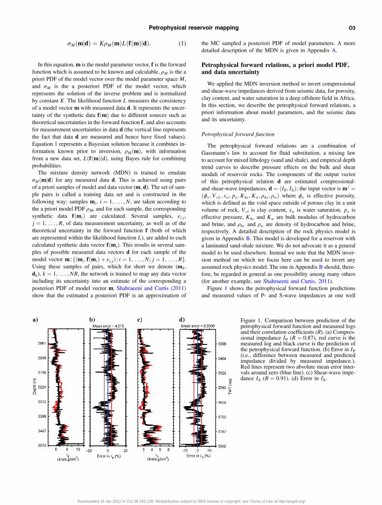
The petrophysical forward relations are a combination ofGassmann’s law to account for fluid substitution, a mixing lawto account for mixed lithology (sand and shale), and empirical depthtrend curves to describe pressure effects on the bulk and shearmoduli of reservoir rocks. The components of the output vectorof this petrophysical relation d are estimated compressional-and shear-wave impedances, d ¼ ðIP; ISÞ; the input vector is m 0 ¼ðϕe; VcL; sw; pe; Khc; Kw; ρhc; ρwÞ where ϕe is effective porosity,which is defined as the void space outside of porous clay in a unitvolume of rock, Vcl is clay content, sw is water saturation, pe iseffective pressure, Khc and Kw are bulk modulus of hydrocarbonand brine, and ρhc and ρw are density of hydrocarbon and brine,respectively. A detailed description of the rock physics model isgiven in Appendix B. This model is developed for a reservoir witha laminated sand-shale mixture. We do not advocate it as a generalmodel to be used elsewhere. Instead we note that the MDN inver-sion method on which we focus here can be used to invert anyassumed rock physics model. The one in Appendix B should, there-fore, be regarded in general as one possibility among many others(for another example, see Shahraeeni and Curtis, 2011).Figure 1 shows the petrophysical forward function predictions

and measured values of P- and S-wave impedances at one well

Figure 1. Comparison between prediction of thepetrophysical forward function and measured logsand their correlation coefficients (R). (a) Compres-sional impedance IP (R ¼ 0.87), red curve is themeasured log and black curve is the prediction ofthe petrophysical forward function. (b) Error in IP(i.e., difference between measured and predictedimpedance divided by measured impedance.).Red lines represent two absolute mean error inter-vals around zero (blue line). (c) Shear-wave impe-dance IS (R ¼ 0.91). (d) Error in IS.

Petrophysical reservoir mapping O3

Downloaded 18 Apr 2012 to 212.39.162.130. Redistribution subject to SEG license or copyright; see Terms of Use at http://segdl.org/

in the field. In that figure errors in the prediction of the petrophy-sical forward function are also shown. The error of the forwardfunction for Ip is around 4% and for Is is around 6%. However,in some intervals, we observe a bias in the prediction of the petro-physical forward function (e.g., 3154–3295 m and 3312–3367 m).It seems that on these intervals the petrophysical forward functionpredictions has a systematic error, which may indicate that the se-lected forward function in Appendix B is not able to model the elas-tic behavior of rock on these intervals. The effect of these errors onthe petrophysical inversion result will be discussed in the “Discus-sion” section.Figure 2 shows crossplots of impedances and effective porosity

color coded by clay content for samples from the well in Figure 1.The predictions of the petrophysical forward function for water sa-turated samples at average effective pressure of the well and fordifferent values of clay content are shown by black curves in thatfigure. These crossplots in addition to error plots in Figure 1 showthat in general the petrophysical forward function is able to modelthe elastic behavior of rocks at the well. However, effect of errorsand uncertainties in the predictions of the petrophysical forwardfunction must be taken into account in the petrophysical inversion.In our inverse problem, the data vector d ¼ ðIP; ISÞ is derived

from the inversion of seismic data, and is inverted for the marginal

joint PDF of the model vector with porosity, clay content, andwater saturation as its components, m ¼ ðϕe; Vcl; swÞ. Otherinput parameters of the petrophysical forward relations are treatedas confounding parameters, mconf ¼ ðPe; Khc; Kw; ρhc; ρwÞ —parameters that may vary and thus alter the uncertainty in estimatedmodel vector m. In mathematical terms, in the MDN solutionthe confounding petrophysical parameters are integrated out inthe marginal a posteriori PDF of the model vector m:

σMðmjdÞ ¼Zmconf

σMðm 0jdÞ dmconf . (2)

Thus, the effect of possible variations of confounding modelparameters on the posterior PDF is integrated out, and this integra-tion results in an increase in uncertainty of the estimated a posteriorimodel vector m ¼ ðϕe; Vcl; swÞ.

Seismic data

A 3D simultaneous elastic inversion technique jointly invertednear-, mid-, and far-angle substacks to derive estimates of the3D distribution of compressional- and shear-wave impedances,IP and IS. Five angle stacks were used as the input seismic data

Figure 2. Crossplot of impedances and porosityfor samples from one well. (a) Compressional im-pedance IP versus effective porosity. Hot colorsrepresent higher values of clay content. Blackcurves represent predictions of the petrophysicalforward function for 100% water saturated sam-ples at the mean effective pressure of the reservoir.(b) Shear-wave impedance IS versus effectiveporosity.

O4 Shahraeeni et al.

Downloaded 18 Apr 2012 to 212.39.162.130. Redistribution subject to SEG license or copyright; see Terms of Use at http://segdl.org/

set, with angle ranges 0°–13° for near, 13°–21° and 21°–29° formiddle, 29°–37° for far, and 37°–45° for ultra-far stacks. The sam-pling interval of the seismic data was 3 ms. The wavelet for eachangle stack was estimated at four different well locations usingreflection coefficients obtained from VP, VS, and density logs.Structural and stratigraphic interpretations resulted in picks of 18

different horizons in the seismic data to define the geometry of theinitial model used for inversion. The a priori models for IP and IS ineach horizon were provided by the low-frequency trend of the welllogs and were extrapolated over the entire model using krigingmethods. The trend of a priori IP and IS were obtained from seismicinterval velocity (provided from seismic imaging) and the distribu-tion of the residuals was obtained from kriging of well logs(Dubrule, 2003, p. 3–39). The range of the variogram used forthe kriging was defined based on a priori geologic informationin each of the 18 different horizons of the model geometry. Theresult of the kriging was then filtered with a low-pass filter (belowseismic band-pass) and transferred into the model geometry as priorIP and IS model. Finally, An iterative algorithm, based on thesimulated annealing technique (Sen and Stoffa, 1991) was usedto adjust this prior model estimates of IP and IS in each bin, to op-timize the match between the input seismic data and the syntheticseismic response calculated by the Zoeppritz equations (Aki andRichards, 1997).

In this way, the seismic-inversion technique combined geologicinformation about the expected vertical and spatial continuity of themedium, well-log data, and information from seismic data to pro-vide an estimate of the distribution of IP and IS. The result for onesection, which includes one of the wells, is shown in Figure 3.Uncertainty of the estimated values of IP and IS can be derived

either directly from the inversion algorithm (Buland et al., 2003;Buland and Omre, 2003) or by statistical comparison between up-scaled IP and IS values derived from well-log and seismic-inversionresults (Bachrach, 2006). In this study, the latter method wasapplied and the a posteriori uncertainty of the inversion for IPwas modeled as a Gaussian distribution with zero mean andstandard deviation of σIP ¼ 0.06 IP, and for IS was modeled as aGaussian distribution with zero mean and standard deviation ofσIS ¼ 0.08 IS. This uncertainty means that if we take several sam-ples of IP with an average value equal to 6000, 68% of the sampleswill be between 5640 and 6360. It is important to note that applica-tion of this method to estimate uncertainty means that IP and ISderived from seismic inversion are assumed to be unbiased. Thisassumption may be violated where the low-frequency backgroundmodel used in inversion is biased. In particular, areas of the fieldwith low-effective stress would be bypassed by low-frequencybackground trend. However, in the area under study in this paperabnormal pressure behavior is not reported and the low-frequency

Figure 3. The P- and S-wave-impedance forone cross section of the 3D seismic data set.(a) Compressional-wave impedance. The correla-tion between inverted samples and upsclaed welllogs is R ¼ 0.88. (b) Shear-wave impedance(R ¼ 0.85). Black curve is the upscaled measuredwell log.

Petrophysical reservoir mapping O5

Downloaded 18 Apr 2012 to 212.39.162.130. Redistribution subject to SEG license or copyright; see Terms of Use at http://segdl.org/

trend is valid. In general, due to the fact that the statistical estimationof uncertainty is based on well data, it can be an underestimation ofthe true uncertainty away from the well.

A priori PDF of the input parameters of the forwardpetrophysical function

To choose the a priori PDF of the model parameters, well-log datafrom the five wells in the field were analyzed. Figure 4a shows the

values of effective porosity versus clay content for well-log samplesfrom the five wells. A correlation between these two parameters canbe observed in that figure. Based on this observation, the a priorimaximum allowable range or interval for effective porosity and claycontent was defined as the region Tðϕe; VclÞ, which is shown inFigure 4a. Figure 4b and 4c shows effective porosity versus watersaturation, and clay content versus water saturation for well-logsamples, respectively. These two figures show that, while effectiveporosity and clay content values are to some extent correlated withwater saturation values, there are no hard boundaries to intervals inwhich parameters lie as there are in Figure 4a. In addition, weobserve that for all samples with clay content values higher than0.8, the water saturation is equal to one. According to theseobservations we assumed a priori that porosity and clay contentwere uniformly distributed over the T-area in Figure 4a. Also,we assumed that a priori water saturation is equal to one when claycontent is higher than 80%, and that it is uniformly distributed overthe [0,1] interval for clay content values lower than 80%. We thusassumed very weak prior information about the three parametersof interest.Effective pressure changes between 173 and 332 bars in the depth

intervals that we considered. We do not observe any correlationbetween effective pressure and effective porosity, clay content, orwater saturation in our data set. However, according to Batzle andWang (1992), the bulk modulus and density of any type of hydro-carbon (with a given value of API degree) are empirical functions ofpore pressure and temperature. The pore pressure and overburdenstress and hence the effective pressure are assumed to be hydro-static. The empirical relation between bulk modulus (or density)of fluid and pore pressure is transformed into a relation betweenbulk modulus (or density) of fluid and effective pressure, usingthe above assumption. Five different types of hydrocarbon, withdifferent API degrees, were observed in the well intervals we con-sidered. For each type, the bulk modulus as a function of effectivepressure, and density as a function of effective pressure, are derivedfrom Batzle and Wang (1992) equations and hydrostatic assump-tion, and shown in Figure 5a and 5b, respectively. The effect ofchange of temperature over the interval of interest on both thehydrocarbon bulk modulus and density was assumed to be negli-gible in this study. Brine density and bulk modulus are equal to1.008 g∕cm3 and 2.625 GPa, respectively, and are constant in allwell intervals we considered. Based on the above observations, ef-fective pressure was assumed to be uniformly distributed between173 and 223 bar, and bulk modulus and density of fluid were de-rived from effective pressure using the straight lines in Figure 5 foreach of the five different types of hydrocarbon.The above a priori probability densities are selected to be as non-

informative (conservative) as possible given the known constraints.However, they limit possible values of the model parameters to phy-sically realizable values in the field in this study. The MDN inver-sion method can be applied with any a priori PDF and the above apriori PDF’s are selected because they are more suitable for the datain this study.

Forward modeling of IP: Effect of confoundingparameters and uncertainties

In this section, we study the effect of variations of the confound-ing parameters and measurement uncertainties on the predictionsof the petrophysical forward function. Figure 6a shows IP as a

Figure 4. Crossplot of the parameters of the model vector. (a) Claycontent versus effective porosity; T represents the a priori region ofthe porosity-clay content plane. (b) Effective porosity versus watersaturation. (c) Clay content versus water saturation.

O6 Shahraeeni et al.

Downloaded 18 Apr 2012 to 212.39.162.130. Redistribution subject to SEG license or copyright; see Terms of Use at http://segdl.org/

function of porosity, when all other input parameters of thepetrophysical forward relations are held constant at possible realis-tic values: Vcl ¼ 0.2, sw ¼ 0.3, pe ¼ 200 bar, Khc ¼ 0.22 GPa,Kw ¼ 2.62 GPa, ρhc ¼ 0.47 g∕ cm3, and ρhc ¼ 1.008 g∕cm3. Theuncertainty in Figure 6a is Gaussian and due to two sources: (1)Uncertainty in the inverted value of IP and IS (i.e., measurementuncertainty) and (2) uncertainty in the predictions of the petrophy-sical forward function (i.e., theoretical uncertainty). The PDF ofuncertainty in the inverted value of seismic IP and IS is Gaussianand is introduced in the section of seismic data above. The PDF ofuncertainty in the predictions of the petrophysical forward functionis also Gaussian and introduced in Appendix B. The total uncer-tainty, which is shown in Figure 6a and 6b is the combined effectof the above two sources of uncertainty. The PDF of this uncertaintyis Gaussian and its covariance matrix is equal to the sum of covar-iance matrices of the above sources of uncertainty (Tarantola, 2005,p. 35). Notice that these plots are different from plots that representthe theoretical uncertainty alone, as might be found in otherpapers (e.g., Tarantola and Valette, 1982). This is because in theMDN inversion methodology, data measurement uncertainties

are also added to the theoretical forward equations uncertainties(Devilee et al., 1999; Meier et al., 2007b; Shahraeeni andCurtis, 2011).Figure 6b shows IP as a function of porosity for the constant

values of clay content and water saturation given above, but whenthe confounding parameters (i.e., effective pressure, bulk modulus,and density of hydrocarbon) are varied according to their a prioridistributions. The thicker black and dark gray area in Figure 6b incomparison with Figure 6a shows that the uncertainty of theprediction of the petrophysical forward function increases due tovariations in the confounding parameters.Figure 6c, 6d, 6e, and 6f shows variation of IP as a function

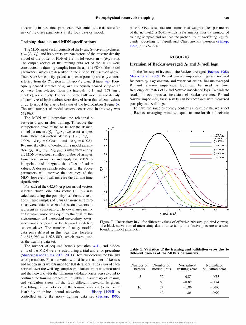
of clay content and water saturation in the same manner as Figure 6aand 6b for porosity. In particular, Figure 6d and 6f shows the effectof variations in the confounding parameters on the uncertaintyof IP.Figure 7 shows a cross section of IP-ϕe for porosity equal to 15%.

Different Gaussians in that figure correspond to uncertainty in IPdue to different values of the confounding parameters (in particulareffective pressure). Note that due to theoretical relationship between

Figure 5. Properties of five different types ofhydrocarbons (with different API degrees) in thewells. (a) Density as a function of effective pres-sure. (b) Bulk modulus as a function of effectivepressure.

Petrophysical reservoir mapping O7

Downloaded 18 Apr 2012 to 212.39.162.130. Redistribution subject to SEG license or copyright; see Terms of Use at http://segdl.org/

effective pressure and P- and S-wave impedance, changes inconfounding model parameters induce a shift in the mean valueof the Gaussians. The black curve represents the sum of differentGaussians and total uncertainty due to uncertainty in the value ofconfounding parameters, measurement uncertainty and uncertaintyin the petrophysical forward function predictions.Figure 6 shows that although IP is a strongly varying function of

porosity and clay content, and a weakly varying function of watersaturation, inference of the petrophysical parameter values from IP

estimates may well be obscured by the high uncertainty of IP due touncertainty in the seismic processing, and due to confounding para-meters of the petrophysical forward relations. In the same manner asfor IP, uncertainty in IS is also high due to aforementioned sourcesand the inference of petrophysical parameters from IS may also bewell obscured. Therefore, with only two data (IP and IS) for threeunknowns (porosity, clay content, and water saturation) we clearlydo not expect a unique solution. Hence, herein we aim principally toassess how much information the seismic data provides to reduce

Figure 6. Uncertainty in the predictions of the petrophysical forward relations for IP. (a) Plot of IP versus porosity when other input parametersof the petrophysical forward relations are held constant. Ambiguity (gray area) is due to the overall effect of theoretical and measurementuncertainty. (b) Plot of IP versus porosity when confounding parameters of the petrophysical forward function are varied. The thicker black anddark gray area show additional uncertainty due to variation of the confounding parameters. (c and d) Corresponding plots for IP versus claycontent. (e and f) Corresponding plots for IP versus water saturation.

O8 Shahraeeni et al.

Downloaded 18 Apr 2012 to 212.39.162.130. Redistribution subject to SEG license or copyright; see Terms of Use at http://segdl.org/

uncertainty in these three parameters. We could also do the same forany of the other parameters in the rock physics model.

Training data set and MDN specifications

The MDN input vector consists of the P- and S-wave-impedancesd ¼ ðIP; ISÞ, and its outputs are parameters of the mixture densitymodel of the posterior PDF of the model vector m ¼ ðϕe; c; swÞ.The output vectors of the training data set of the MDN wereconstructed by drawing samples from the a priori PDF of the modelparameters, which are described in the a priori PDF section above.There were 846 equally spaced samples of porosity and clay contentselected from the T-region in the ϕe-Vcl plane (Figure 4a). Fortyequally spaced samples of sw and six equally spaced samples ofpe were then selected from the intervals [0,1] and [173 bar ,332 bar], respectively. The values of the bulk modulus and densityof each type of hydrocarbon were derived from the selected valuesof pe to model the elastic behavior of the hydrocarbon (Figure 5).The total number of model vectors constructed in this way was642,960.The MDN will interpolate the relationship

between d and m after training. To reduce theinterpolation error of the MDN for the desiredmodel parameters (ϕe, Vcl, sw) we select samplesfrom these parameters densely (i.e., Δϕe ¼0.009, ΔVcl ¼ 0.0204, and Δsw ¼ 0.025).Because the effect of confounding model param-eters (pe, Khc, ρhc, Kw, ρw) is integrated out bythe MDN, we select a smaller number of samplesfrom these parameters and apply the MDN tointerpolate and integrate the effect of othervalues. A denser sample selection of the aboveparameters will improve the accuracy of theMDN; however, it will increase the training timesignificantly.For each of the 642,960 a priori model vectors

selected above, one data vector (IP, IS) wascalculated using the petrophysical forward rela-tions. Three samples of Gaussian noise with zeromean were added to each of these data vectors torepresent data uncertainty. The covariance matrixof Gaussian noise was equal to the sum of themeasurement and theoretical uncertainty covar-iance matrices given in the forward modelingsection above. The number of noisy model-data pairs derived in this way was therefore3 × 642; 960 ¼ 1; 928; 880, which were usedas the training data set.The number of required kernels (equation A-1), and hidden

units of the MDN were selected using a trial and error procedure(Shahraeeni and Curtis, 2009, 2011). Here, we describe the trial anderror procedure. Four networks with different number of kernelsand hidden units were trained for 100 iterations. Then error of eachnetwork over the well-log samples (validation error) was measuredand the network with the minimum validation error was selected tocontinue the training procedure. In Table 1, a summary of trainingand validation errors of the four different networks is given.Overfitting of the network to the training data set (a source ofinstability in trained neural networks — Bishop [1995]) iscontrolled using the noisy training data set (Bishop, 1995,

p. 346–349). Also, the total number of weights (free parametersof the network) is 2041, which is far smaller than the number oftraining samples and reduces the probability of overfitting signifi-cantly according to Vapnik and Chervonenkis theorem (Bishop,1995, p. 377–380).

RESULTS

Inversion of Backus-averaged IP and IS well logs

In the first step of inversion, the Backus-averaged (Backus, 1962;Mavko et al., 2009) P- and S-wave impedance logs are invertedfor porosity, clay content, and water saturation. Backus-averagedP- and S-wave impedance logs can be used as low-frequency estimates of P- and S-wave impedance logs. To evaluateresults of petrophysical inversion of Backus-averaged P- andS-wave impedance, these results can be compared with measuredpetrophysical well logs.To have the same frequency content as seismic data, we select

a Backus averaging window equal to one-fourth of seismic

Table 1. Variation of the training and validation error due todifferent choices of the MDN’s parameters.

Number ofkernels

Number ofhidden units

Normalizedtraining error

Normalizedvalidation error

5 52 −0.87 −0.7380 −0.89 −0.74

10 27 −1.00 −0.9040 −1.05 −0.90

Figure 7. Uncertainty in IP for different values of effective pressure (colored curves).The black curve is total uncertainty due to uncertainty in effective pressure as a con-founding model parameter.

Petrophysical reservoir mapping O9

Downloaded 18 Apr 2012 to 212.39.162.130. Redistribution subject to SEG license or copyright; see Terms of Use at http://segdl.org/

wavelength. The average seismic wave frequency in the seismicdata in this application is around 20 Hz and the average wave speedis around 2800 m∕s, henceforth the wavelength is around 140 m.This wavelength is much larger than the typical thickness of layersin the well (at most 4 m) and, therefore, Backus averaging can beused to estimate the behavior of seismic wave. The Backus aver-aging window used was approximately one-fourth of the above seis-mic wavelength, which is around 35 m. Figure 8a and 8b shows themeasured and Backus-averaged IP and IS for one well.For the inversion of the Backus-averaged IP and IS logs, uncer-

tainty of data was assumed to be equal to the uncertainty of thepetrophysical forward function (Appendix A), and a priori informa-tion about model parameters was assumed to be the same as thosedescribed in the method section above. Another training data setwas constructed using the same procedure as explained above.We trained a separate MDN with the above data set and applied it

to invert Backus-averaged IP and IS logs to obtain the a posterioriPDF of porosity, clay content, and water saturation logs. The results

are shown in Figure 8c, 8d, and 8e, for porosity, clay content, andwater saturation, respectively. Note that a relatively large bias in thevalue of clay content can be observed on the 3540–3640 ms inter-val. Figure 1 shows that the predictions of the petrophysical forwardfunction are also biased on this interval. This observation means thatapplying the petrophysical forward function for inversion can resultin large errors on the aforementioned interval.

Inversion of seismic IP and IS

The MDN with the specifications given above was trained usingthe training data set fðmk; dkÞ∶k ¼ 1; : : : ; NRg to estimate the jointPDF of model vectorm ¼ ðϕe; c; swÞ from data vector d ¼ ðIP; ISÞ.In this section, we present results of the inversion of seismicIP and IS.Figure 9 shows the joint marginal PDF’s of model parameters

evaluated at a randomly chosen data point at one well in the fieldwith IP ¼ 7345 kg∕ðm2sÞ and IS ¼ 4658 kg∕ðm2sÞ. The measured

Figure 8. Comparison of the maximum a poster-iori marginal PDF of petrophysical parametersobtained from inversion of the backus-averagedIP and IS logs and measured logs. (a) MeasuredIP (black) and Backus-averaged IP (red); (b) IS.(c) Measured porosity (black) and inverted poros-ity (red). (d) Clay content. (e) Water saturation.

O10 Shahraeeni et al.

Downloaded 18 Apr 2012 to 212.39.162.130. Redistribution subject to SEG license or copyright; see Terms of Use at http://segdl.org/

values of model parameters for this data point are ϕe ¼ 0.19,c ¼ 0.04, and, sw ¼ 0.13, which are shown by crosses in Figure 9.The point estimates of porosity, clay content, and water saturationare obtained as the MAP points of the marginal PDF’s and are equalto 0.17 for porosity, 0.04 for clay content, and 0.12 for watersaturation.To assess reduction of uncertainty in the model parameters after

inversion, which is due to additional information in seismic data, wecompare the posterior and the prior standard deviations. Thestandard deviation for the posterior PDF’s of porosity, clay content,and water saturation are equal to 0.02, 0.05, and 0.17, respectively,while for the prior PDF’s they are equal to 0.09, 0.26, and 0.30,respectively. The relative reduction in all three posterior standarddeviations shows that the inversion process decreases the uncer-tainty of all model parameters. Remaining uncertainty in the modelparameters is mainly due to uncertainty in effective pressure, otherconfounding parameters, theoretical uncertainty and error of thepetrophysical forward relations, and error in IP and IS estimatesobtained from seismic data. Note that, in general, reduction ofuncertainty of water saturation is much smaller than reduction ofuncertainty of porosity and clay content.Figures 10 and 11 show the marginal PDF’s of porosity,

clay content, and water saturation, derived from the inversion ofseismic IP and IS in two intervals along the well profile (perfor-mance at other wells is similar). The value of water saturation inthese two intervals varies between 10% and 100%. The first rowsin Figures 10 and 11 show results of the MDN inversion of seismicdata. To assess the accuracy of the MDN solution, an MC samplingmethod was also applied to solve the same inverse problem on theabove intervals. The a priori information about model parametersand the petrophysical forward relations used in the MC samplinginversion were the same as the MDN inversion. The marginal PDF’sof the model parameters, which are obtained from MC sampling,are shown in the second row of Figures 10 and 11. Comparisonbetween the results of the MDN inversion and MC sampling inver-sion shows that the MDN solution gives an acceptable approxima-tion of the MC sampling solution. Shahraeeni and Curtis (2011)show other examples of the comparison between MC samplingand MDN inversion result. In those examples also, the MDN inver-sion results are acceptable estimates of MC sampling results. It canbe argued that in some cases MDN results are better estimates of thelow-resolution logs than MC sampling results; this might be due tothe learning ability of neural networks.In Figures 10 and 11, in addition to the marginal PDF’s of the

model parameters, a solid black line shows the result of inversion ofBackus-averaged IP and IS. A solid red line shows the maximum aposteriori (MAP) of the marginal PDF’s of the model parameters.Figures 10 and 11 show that the marginal PDF’s of the modelparameters derived from inversion of seismic IP and IS representgood estimates of the inversion result of Backus-averaged IP andIS. In particular, the MAP of the marginal PDF’s (solid red linesin Figures 10 and 11) estimates the inversion result of Backus-averaged IP and IS with a reasonable accuracy. The differencebetween the values of porosity, clay content, and water saturationderived from seismic IP and IS and the values of these parametersderived as the MAP of the inversion of Backus-averaged IP and IScan be due to errors in the processing of the seismic data.Figure 12a shows the MAP of porosity after inverting the IP

and IS cross sections in Figure 3. Figure 12b shows the standard

deviation of the marginal distribution of porosity in this crosssection. The highest value of the color bar corresponds to the apriori standard deviation of porosity, and throughout the cross sec-tion the a posteriori standard deviation is smaller than this value (thecolor of the a priori standard deviation is red, and the hottest color inFigure 12b is light orange). Figures 13a and 14a show the MAP ofclay content and water saturation, respectively, after inverting IP

Figure 9. Marginal a posteriori joint PDF of model parametersfor IP ¼ 7345 ðkm∕sÞ.ðg∕cm3Þ and IS ¼ 4658 ðkm∕sÞ.ðg∕cm3Þ.(a) Marginal joint PDF of effective porosity and clay content.(b) Marginal joint PDF of clay content and water saturation.(c) Marginal joint PDF of effective porosity and water saturation.Hot colors show high probability zones. The black cross is the valueof logs for this data point.

Petrophysical reservoir mapping O11

Downloaded 18 Apr 2012 to 212.39.162.130. Redistribution subject to SEG license or copyright; see Terms of Use at http://segdl.org/

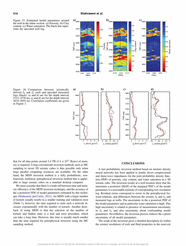
and IS sections in Figure 3. Figures 13b and 14b show the standarddeviations of clay content and water saturation in each section.Again, the highest values of the color bars correspond to the a prioristandard deviation values, and it is evident that for all data points thea posteriori standard deviation is smaller than this value.Figure 15 shows the MAP of model parameters for 30 neighbor-

ing traces of the well in the inline section perpendicular to theprevious crossline section. Figures 12, 13, and 14, in addition toFigure 15 show this method gives a good 3D estimate of theunderground rock and fluid properties. As indicated previously,in addition to the MAP and standard deviation estimate of the modelparameters, any other statistical property of the model parameterscan be calculated from the estimated conditional joint PDFpðϕe; c; swjIP; ISÞ, for any location spanned by the 3D seismicdata sets.

DISCUSSION

Figures 10 and 11 show that the MAP’s of the marginal a poster-iori PDF of the model parameters are reasonable estimates of thevalues obtained from the inversion of the Backus-averaged logs.The error in the petrophysical inversion of seismic IP and IS canbe related to uncertainty in the inverted seismic data and theaccuracy of the petrophysical forward relations.

Figure 1 shows the measured well log of IP and IS and corre-sponding predictions of the petrophysical forward relations. Largebiases in the predictions of the petrophysical forward relations canbe seen in the interval 3550–3700 ms. These biases result in errorsin the estimated values of porosity, clay content, and water satura-tion obtained from inversion of Backus-averaged IP and ISin Figure 8. In particular, we can see biases in the estimatedclay content value on the same interval in that figure. The errorover the above interval shows the effect of the accuracy of the pet-rophysical forward relations on the petrophysical inversion result.Appendix B shows that Reuss average of the elastic moduli of sandand shale and Gassmann theory are applied to derive the petrophy-sical forward function. The Reuss average is a lower bound of theelastic moduli of a mixture of rocks; therefore, the petrophysicalforward function may underestimate the equivalent elastic moduliof the mixture of sand and shale. Application of more accurate the-oretical models might improve the accuracy of the petrophysicalforward function and reduce error in the petrophysical inversionresult.Figure 16a and 16b shows IP and IS obtained from seismic

data and compare it with Backus-averaged logs for the two inter-vals in Figures 10 and 11. This figure shows that seismic inversionfor IS in the interval 3425–3470 ms has large errors (in some

Figure 10. Marginal a posteriori PDF’s of themodel parameters from the inversion of seismi-cally derived IP and IS for the depth interval3335–3555 ms, in one of the wells. First row isthe marginal PDF of the model parameters ob-tained using MDN: (a) Porosity (R ¼ 0.86).(b) Clay content (R ¼ 0.80). (c) Water saturation(R ¼ 0.84). Second row is the joint PDF of themodel parameters usingMC sampling: (d) Porosity(R ¼ 0.86). (e) Clay content (R ¼ 0.80). (f) Watersaturation (R ¼ 0.84). Solid black line is the low-resolution log. Darker areas show high probabilityzones. The solid red line is the maximum a poster-iori (MAP) of the marginal PDFs; R in each itemshows the correlation coefficient between theMAP and low-resolution log.

O12 Shahraeeni et al.

Downloaded 18 Apr 2012 to 212.39.162.130. Redistribution subject to SEG license or copyright; see Terms of Use at http://segdl.org/

cases near 25%, around two times larger than the 14% errorused in the MDN inversion above). This error results in largeerrors in the inverted values of porosity and clay content on thesame interval in Figure 10a and 10b. We also see large errors inthe inverted values of IP in the shale interval 3500–3550 ms,which result in errors in the inverted values of clay content onthe same interval in Figure 10b. The errors in the above intervalsshow the effect of the accuracy of the processed seismic dataon the petrophysical inversion result. Any improvement in theaccuracy of the inverted seismic data can reduce the effect of thistype of error.The MDN inversion method relies on the validity of the seismic

impedance inversion. Due to several sources of uncertainty such aswavelet parameters, seismic-to-well tie, low-frequency a priori im-pedance model, and amplitude processing, the seismic inversion canbe biased and inaccurate away from the well. However, due to timeefficiency of the MDN inversion method, it is possible to applythis method with multiple realizations of IP and IS obtained byprobabilistic inversion of seismic data. In such cases, for eachrealization, the MDN gives the joint PDF of the petrophysicalparameters. The average of these PDF’s can be used as a petrophy-sical model that captures uncertainties due to uncertainties in theelastic inversion process.

Figures 9, 10, and 11 show the a posteriori uncertainty ofporosity, clay content, and water saturation is large. The highuncertainty of model parameters stems from uncertainty about con-founding model parameters (i.e., effective pressure, bulk modulus,and density of hydrocarbon), uncertainty of the petrophysical for-ward relations, and measurement uncertainty in seismic IP and IS.In addition of course, we invert only two data for three parameters,and hence, simply by appealing to dimensionality arguments, aunique solution is impossible without strong a priori information.Figures 6 and 7 show the effect of theoretical and measurementuncertainty in addition to the effect of the confounding modelparameters on the uncertainty of IP (the behavior of IS is similar).In particular, for water saturation, in Figure 6f, we observe thatuncertainty in the confounding model parameters results in largeuncertainty in IP values. Figure 6f shows that even when porosityand clay content values are known, for a given value of IP theuncertainty of water saturation is large. This means that the reduc-tion in uncertainty in the water saturation from the petrophysicalinversion will always be small (Figures 9, 10, and 11). Bachrach(2009) and Spikes (2007) report the same high uncertainty for aposteriori water saturation in petrophysical inversion. Nevertheless,the inversion process does reduce the uncertainty of all modelparameters as can be seen in Figures 12b, 13b, and 14b.

Figure 11. Marginal a posteriori PDFs of themodel parameters from the inversion of seismi-cally derived IP and IS for the depth interval3674–3855 ms in one of the wells. First row isthe marginal PDF of the model parameters ob-tained using MDN: (a) Porosity. (b) Clay content.(c) Water saturation. Second row is the joint PDFof the model parameters using MC sampling:(d) Porosity. (e) Clay content. (f) Water saturation.Solid black line is the low-resolution log. Darkerareas show high probability zones. The solid redline is the maximum a posteriori (MAP) of themarginal PDF’s. Correlation coefficients betweenlow-resolution logs and MAP estimates are thesame as those shown in Figure 10.

Petrophysical reservoir mapping O13

Downloaded 18 Apr 2012 to 212.39.162.130. Redistribution subject to SEG license or copyright; see Terms of Use at http://segdl.org/

Figures 12a, 13a, and 14a in conjunction with Figure 15 showthat if this method is applied to invert 3D seismic IP and IS sections,the estimates of porosity, clay content, and water saturation canprovide a detailed 3D description of rock properties in a reservoir.This is of great value and importance for exploration and reservoirdevelopment plans as it can help to locate possible sources ofhydrocarbon inside a reservoir. The accuracy and resolution of thisdescription depends on the accuracy and resolution of 3D seismicimpedance cubes, and on the accuracy of the petrophysical relation-ships used.In some reservoirs, it is possible to observe rocks with different

petrophysical properties (i.e., porosity and clay content) and similarvalues of IP and IS (Shahraeeni and Curtis, 2011). In such cases,due to multimodal nature of a posteriori PDF of the petrophysicalproperties, applying conventional fast probabilistic inversion meth-ods (e.g., linearized inversion with Gaussian assumption about priorand posterior uncertainties [Rimstad and Omre, 2010]) can result inlarge errors in the estimated value of porosity and clay content.Shahraeeni and Curtis (2011) show that in those cases MDN canestimate the a posteriori PDF of the petrophysical parameters withacceptable accuracy. Also, we must note that the technique pre-sented by Rimstad and Omre (2010) is very efficient and useful

for integration of geological prior information in the petrophysicalinversion procedure.Due to large uncertainty associated with data, petrophysical

forward relations, and confounding model parameters, the a poster-iori PDF of model parameters, and especially water saturationwill always have large uncertainty. To address this uncertaintyappropriately, any petrophysical inversion method must be prob-abilistic. The MDN method is a time- and memory-efficient meth-od for probabilistic nonlinear inversion. The nonlinear inversion ofeach crossline section, which included 170,322 data points andresulted in the full joint posterior PDFs of ϕe, c, and sw, only took340 s on a regular desktop computer. The number of crossline sec-tions is 1461, so inverting the whole 3D seismic cube with248,840,442 data points takes only around 138 hours on the samedesktop computer. Note that solving the same number of petrophy-sical inverse problems using the MC sampling method will takearound 27,500 hours on the same desktop computer (nearly200 times more than MDN). What is more, the mixture densityneural network encoded the full joint PDF of all model parametersfor all data points into only 2041 scalar values (i.e., the number ofMDN weights), which requires 20.5 KB memory for storage. Thestorage of the MC sampling results requires 3.2 MB, which means

Figure 12. Estimated porosity and its associateduncertainty for one section from the seismic cube,which includes one of the wells. (a) Maximum aposteriori of the marginal PDF of porosity.(b) Standard deviation of porosity. The black linerepresents the upscaled well log.

O14 Shahraeeni et al.

Downloaded 18 Apr 2012 to 212.39.162.130. Redistribution subject to SEG license or copyright; see Terms of Use at http://segdl.org/

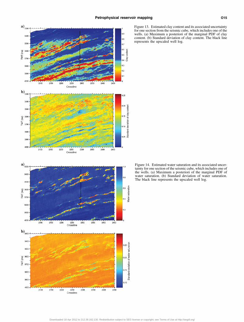
Figure 13. Estimated clay content and its associated uncertaintyfor one section from the seismic cube, which includes one of thewells. (a) Maximum a posteriori of the marginal PDF of claycontent. (b) Standard deviation of clay content. The black linerepresents the upscaled well log.

Figure 14. Estimated water saturation and its associated uncer-tainty for one section of the seismic cube, which includes one ofthe wells. (a) Maximum a posteriori of the marginal PDF ofwater saturation. (b) Standard deviation of water saturation.The black line represents the upscaled well log.

Petrophysical reservoir mapping O15

Downloaded 18 Apr 2012 to 212.39.162.130. Redistribution subject to SEG license or copyright; see Terms of Use at http://segdl.org/

that for all data points around 2.4 TB (2.4 × 1012 Bytes) of mem-ory is required. Using conventional inversion methods such as MCsampling to invert 3D seismic cubes is thus possible only whenlarge parallel computing resources are available. On the otherhand, the MDN inversion method is a fully probabilistic, non-Gaussian, nonlinear, petrophysical inversion method that is applic-able to large seismic cubes on a standard desktop computer.We must consider that there is a trade-off between time and mem-

ory efficiency of the MDN inversion technique, and the accuracy ofthe a posteriori PDF of model parameters estimated by this techni-que (Shahraeeni and Curtis, 2011). An MDN with a larger numberof kernels usually results in a smaller training and validation error(Table 1), however, the time required to train such a network in-creases exponentially with the number of kernels. Another draw-back of using MDN is that the selection of the number ofkernels and hidden units is a trial and error procedure, whichcan take a long time. However, this time is usually much smallerthan the time required for petrophysical inversion using the MCsampling method.

CONCLUSIONS

A fast probabilistic inversion method based on mixture densityneural networks has been applied to jointly invert compressionaland shear-wave impedances for the joint probability density func-tion (PDF) of porosity, clay content, and water saturation in a 3Dseismic cube. The inversion results at a well location show that themaximum a posteriori (MAP) of the marginal PDF’s of the modelparameters is a reasonable estimate of corresponding low-resolutionlog. Residual errors correspond to errors in the petrophysical for-ward relations, and differences between the seismic IP and IS andmeasured logs at wells. The uncertainty in the a posteriori PDF ofthe model parameters and in particular water saturation is high. Thishigh uncertainty is related to presence of measurement uncertaintyin IP and IS and also uncertainty about confounding modelparameters. Nevertheless, the inversion process reduces the a prioriuncertainty of all model parameters.The result of the inversion gives a detailed description (to within

the seismic resolution) of rock and fluid properties in the reservoir

Figure 15. Estimated model parameters aroundthe well in the inline section. (a) Porosity. (b) Claycontent. (c) Water saturation. The black line repre-sents the upscaled well log.

Figure 16. Comparison between seismicallyderived IP and IS (red) and upscaled measuredlogs (black). (a and b) are for the depth interval3333–3570 ms. (c and d) are for the depth interval3674–3855 ms. Correlation coefficients are givenin Figure 3.

O16 Shahraeeni et al.

Downloaded 18 Apr 2012 to 212.39.162.130. Redistribution subject to SEG license or copyright; see Terms of Use at http://segdl.org/

that can be used for exploration and development planning. Inparticular, it can be used to find areas with high effective porosityand low clay content (pay zones), and also areas with possiblesources of hydrocarbon based on the estimated water saturation.The advantages of the mixture density neural network inversion

method over other probabilistic inversion methods are its memoryand computational efficiency. Due to the large size of 3D seismiccubes, these two properties are essential for any nonlinear probabil-istic petrophysical inversion. As the inversion method is indepen-dent of the particular seismic attributes chosen in this case study (IPand IS), it can be used to invert any set of pertinent seismic attributessuch as compressional- and shear-wave velocity and bulk density, orcompressional impedance and Poisson’s ratio. The main drawbackof using MDN is the trial and error procedure of selecting thenumber of kernels and hidden units.

ACKNOWLEDGMENTS

We would like to thank TOTAL E&P UK for sponsoring thiswork. We acknowledge the support from the Scottish FundingCouncil for the joint research institute with the Heriot-Watt Univer-sity, which is a part of Edinburgh Research Partnership in Engineer-ing and Mathematics (ERPEM).

APPENDIX A

MIXTURE DENSITY NETWORK

One application of neural networks is to estimate some givenmapping from an input vector x to a target vector t. Any uncertaintyassociated with the target vector in this mapping can be representedby the probability density of t conditioned on (or given) x, written aspðtjxÞ. The MDN is a type of neural network that can be trained toemulate an approximation to pðtjxÞ. Within the MDN, pðtjxÞ isrepresented by a mixture or sum of known probability densities:

pðtjxÞ ¼Xmi¼1

αiðxÞφiðtjxÞ. (A-1)

In equation A-1, φiðtjxÞ is a known PDF called a kernel, m is thenumber of kernels, and αiðxÞ is the mixing coefficient that definesthe weight of each kernel in the mixture (the sum). This representa-tion of the PDF is called a mixture model.A mixture of densities with Gaussian kernels can approximate

any PDF to any desired accuracy, given a sufficient number of ker-nels with appropriate parameters (Shahraeeni and Curtis, 2011). Weassume kernels are Gaussian with a diagonal covariance matrix:

φiðtjxÞ ¼1

Qcl¼1

� ffiffiffiffiffi2π

pσilðxÞ

� exp

�−1

2

Xcl¼1

ðtl − μilðxÞÞ2σ2ilðxÞ

�;

(A-2)

where c is the dimensionality of the output vector t ¼ ðt1; : : : ; tcÞ,μilðxÞ is the lth component in the mean vector of the ith kernel, andσil is the lth diagonal element in the covariance matrix of the ithkernel. Therefore, the mean and covariance of the ith Gaussiankernel are μi ¼ ðμi1; : : : ; μicÞ, and Σi ¼ diagðσ2i1; : : : ; σ2icÞ,respectively.Appropriate values for the parameters of the MDN (i.e.,

mixing coefficients, mean and covariance matrix of kernels) in

equations A-1 and A-2 can be predicted by using any standard neur-al network (Bishop, 1995). We apply a two-layer feed-forwardneural network with a single hidden layer of hyperbolic tangentfunctions and an output layer of linear functions.In the network training phase, n statistically independent pairs of

example input and output vectors fxj; tjg are used as training sam-ples. Unknown parameters of the network, which are referred to asweights, are determined in such a way that the likelihood ofthe training samples with respect to the density function inequation A-1 is maximized. The maximization of the likelihoodis equivalent to minimization of the error function E, defined as

E ¼Xnj¼1

Ej ¼ −Xnj¼1

ln pðtjjxjÞ. (A-3)

To find the minimum of E, an optimization algorithm calledscaled conjugate gradient is used. This algorithm determines theminimum of E with respect to the weights of the network, itera-tively. In each iteration the algorithm requires derivatives of E withrespect to the network weights, which are derived by using the so-called back-propagation algorithm (see Bishop (1995) for an expla-nation of the optimization and back-propagation algorithms).Shahraeeni and Curtis (2011) show two examples of MDN

solution of inverse problems and compare results with Monte Carlo(MC) sampling solution. Their results show that MDN can estimateMC sampling solution with an acceptable accuracy.

APPENDIX B

PETROPHYSICAL FORWARD RELATIONS

The petrophysical forward function is a set of mathematicalequations that links the petrophysical parameters of a rock to itselastic parameters (i.e., P- and S-wave velocity and density). Manyparameters can have an influence on the elastic parameters of a rockincluding porosity, size and shape of grains, clay content, fluidsaturation, type of mineral matrix, sorting and arrangement ofgrains, effective pressure, temperature, burial, and history of therock (i.e., diagenesis, tectonics, etc.). In this study, the approachto the petrophysical forward function construction is to explainthe influence of these parameters on the elastic properties as muchas possible.In the field under study, we only observe turbidite sands within

shaley intervals. In this field, shaley intervals are defined as inter-vals with clay volume larger than 60%, and effective porosity lowerthan 5%. First, we develop the petrophysical forward function forthe shaley intervals. Shales are normally not cemented and siltgrains are suspended in the clay matrix of shales (Avseth, 2005).In this case, Reuss average can be used to estimate the elastic mod-uli of shale layers:

Ksh ¼�1 − Vcl

Kqz

þ Vcl

Kclay

�−1

(B-1)

μsh ¼�1 − Vcl

μqzþ Vcl

μclay

�−1

(B-2)

In the above equations, Vcl is clay content, Kqz and μqz are bulkand shear moduli of silts, which are assumed to be mainly

Petrophysical reservoir mapping O17

Downloaded 18 Apr 2012 to 212.39.162.130. Redistribution subject to SEG license or copyright; see Terms of Use at http://segdl.org/

composed of quartz, Kclay and μclay are the correspondingparameters of fluid saturated clay particles, and Ksh and μsh arethe corresponding parameters of shales.We applied the approach of Meadows et al. (2005) to model Kclay

and μclay as empirical functions of effective porosity and effectivepressure. We slightly modified the aforementioned approach byusing effective porosity instead of total porosity. However, dueto the fact that this approach is an empirical approach, this modi-fication would not impose any additional error on the modeled elas-tic parameters of clay. Well-log data on the shaley intervals areapplied to calibrate the empirical relationships. In this sense the pet-rophysical forward function is empirical.Second, we develop the petrophysical forward function for sand

intervals. In sand intervals, clay particles are assumed to be dis-persed in the sand matrix and therefore total porosity can berepresented as a function of effective porosity and clay content:

ϕ ¼ ϕe

1 − Vcl. (B-3)

In the above equation, ϕ is total porosity, and ϕe is effectiveporosity.Following the approach of Nur et al. (1995), bulk and shear

moduli of dry sand, Kdry and μdry, is modeled as

Kdry ¼ Kqz

�1 −

ϕ

ϕc

�; (B-4)

μdry ¼ μqz

�1 −

ϕ

ϕc

�. (B-5)

In the above equation, ϕcis critical porosity. The ratio ϕ∕ϕc isrepresented as an empirical function of effective pressure andporosity (Chao, 2009). The above empirical functions are calibratedwith well-log data. Based on the available data at wells, the effectof other potentially influential parameters such as temperature ordiagenesis is assumed to be negligible in this petrophysical forwardfunction. The existence of such effects in some areas of the fieldwill result in inaccurate predictions of the petrophysical forwardfunction.In this study, we assume that rocks are macroscopically

homogenous, pores are interconnected, fluid is frictionless, andthe rock-fluid system is closed. Therefore, Gassmann theory canbe used to perform fluid substitution for different values of watersaturation (Wang, 2001). Using the bulk and shear moduli of drysand in equations B-4 and B-5, we obtain the following equations:

Ksand ¼ Kdry þ�1 −

Kdry

Kqz

�2

∕�ϕ

Kf

þ ð1 − ϕÞKqz

þ Kdry

K2qz

�;

(B-6)

μsand ¼ μdry: (B-7)

Here Kf is the bulk modulus of saturating fluid.The pore fluid bulk modulus Kf is the bulk modulus of the mix-

ture of water and hydrocarbon inside the effective pore space. By

assuming a homogeneous mixture of water and hydrocarbon, thisbulk modulus is obtained as

Kf ¼�SWKW

þ 1 − SWKH

�−1. (B-8)

In the above equation, SW is water saturation, KW is the bulkmodulus of brine, and KH is the bulk modulus of hydrocarbon.The interconnectivity of pores in shale is questionable, andtherefore, application of Gassmann for them can result in errors.However, in this study we observe that the effect of this errorcan be neglected. More accurate petroelastic models might be usedto model the behavior of shale and therefore reduce errors.geologic observations at the well locations suggest that sand-

shale mixtures in this field are mainly laminated. The petrophysicalforward function for a laminated sand-shale mixture is derived byassuming that laminas are arranged perpendicular to the direction ofwave propagation (Dvorkin and Gutierrez, 2001). For this arrange-ment, the bulk and shear moduli of sand-shale mixture are derivedby Backus averaging of the bulk and shear moduli of sand and shalelaminas:

Kmix ¼�1 − Vcl

Ksand

þ Vcl

Kshale

�−1; (B-9)

μmix ¼�1 − Vcl

μsandþ Vcl

μshale

�−1. (B-10)

Note that the above two equations are the Reuss average of elasticmoduli of sand and shale laminas, which is a lower bound of theelastic moduli of laminas. Therefore, if the perpendicular wave in-cident assumption is violated in the laminated sand-shale mixture,application of the above formulas result in an underestimate of theequivalent elastic moduli of the mixture.Assuming that the earth is isotropic and linearly elastic, the

seismic behavior of sediments can be completely characterizedby three parameters: bulk modulus, shear modulus, and bulk den-sity. Bulk density ρmin is calculated as the volumetric average ofdensity of solid phase and liquid phase. The P- and S-wave impe-dances are derived from the bulk and shear moduli of saturated rock(equation B-9, B-10), and bulk density:

IP ¼ffiffiffiffiffiffiffiffiffiffiffiffiffiffiffiffiffiffiffiffiffiffiffiffiffiffiffiffiffiffiffiffiffiffiffiffiffiffiffiffiffiffiρmixðKmix þ 4∕3μmixÞ

p; (B-11)

IS ¼ffiffiffiffiffiffiffiffiffiffiffiffiffiffiffiffiffiρmix μmix

p. (B-12)

The above petrophysical forward relations are calibrated withdata from eight wells in the field under study to construct thepetrophysical forward function used in the inversion process.Because the petrophysical forward function is calibrated on sev-

eral wells, its uncertainty can be large. For high effective pressure(more than 100 bar) these uncertainties can be modeled by a Gaus-sian PDF with zero mean and standard deviation of 4% for IP and of6% for IS (Chao et al., 2009).

O18 Shahraeeni et al.

Downloaded 18 Apr 2012 to 212.39.162.130. Redistribution subject to SEG license or copyright; see Terms of Use at http://segdl.org/

REFERENCES

Aki, K., and K. P. G. Richards, 1997, Quantitative seismology: Theory andmethods: University Science Books.

Avseth, P., T. Mukerji, A. Jorstad, G. Mavko, and T. Veggeland, 2001,Seismic reservoir mapping from 3-D AVO in a North Sea Turbidite sys-tem: Geophysics, 66, 1157–1176, doi: 10.1190/1.1487063.

Avseth, P., T. Mukerji, and G. Mavko, 2005, Quantitative seismic interpre-tation: Applying rock physics tools to reduce interpretation risk:Cambridge University Press.

Bachrach, R., 2006, Joint estimation of porosity and saturation usingstochastic rock-physics modeling: Geophysics, 71, no. 5, O53–O63,doi: 10.1190/1.2235991.

Backus, G. E., 1962, Long-wave elastic anisotropy produced by horizontallayering: Journal of Geophysical Research, 67, 4427–4440, doi: 10.1029/JZ067i011p04427.

Batzle, M., and M. Z. Wang, 1992, Seismic properties of pore fluids:Geophysics, 57, 1396–1408, doi: 10.1190/1.1443207.

Bishop, C. M., 1995, Neural networks for pattern recognition: OxfordUniversity Press.

Bosch, M., L. Cara, J. Rodrigues, A. Navarro, and M. Diaz, 2007, A MonteCarlo approach to the joint estimation of reservoir and elastic parametersfrom seismic amplitudes: Geophysics, 72, no. 6, O29–O39, doi: 10.1190/1.2783766.

Bosch, M., C. Carvajal, J. Rodrigues, A. Torres, M. Aldana, and J. Sierra,2009, Petrophysical seismic inversion conditioned to well-log data: Meth-ods and application to a gas reservoir: Geophysics, 74, no. 2, O1–O15,doi: 10.1190/1.3043796.

Bosch, M., T. Mukerji, and E. Gonzalez, 2010, Seismic inversion forreservoir properties combining statistical rock physics and geostatistics:A review: Geophysics 75, no. 5, 75A165–75A176, doi: 10.1190/1.3478209.

Buland, A., O. Kolbjornsen, R. Hauge, O. Skjaeveland, and K. Duffaut,2008, Bayesian lithology and fluid prediction from seismic prestack data:Geophysics, 73, no. 3, C13–C21, doi: 10.1190/1.2842150.

Buland, A., O. Kolbjornsen, and H. Omre, 2003, Rapid spatially coupledAVO inversion in the Fourier domain: Geophysics, 68, 824–836, doi:10.1190/1.1581035.

Buland, A., and H. Omre, 2003, Bayesian linearized AVO inversion: Geo-physics, 68, 185–198, doi: 10.1190/1.1543206.

Chao, G., G. Lambert, and H. Cumming, 2009, Analysis of intrinsic uncer-tainties of petro-elastic models using simulated annealing: 71st EAGEConference & Exhibition.

Devilee, R. J. R., A. Curtis, and K. Roy-Chowdhury, 1999, An efficient,probabilistic neural network approach to solving inverse problems: Invert-ing surface wave velocities for Eurasian crustal thickness: Journal ofGeophysical Research, 104, 28841–28857, doi: 10.1029/1999JB900273.

Doyen, P. M., 1988, Porosity from seismic data: A geostatistical approach:Geophysics, 53, 1263–1275, doi: 10.1190/1.1442404.

Dubrule, O., 2003, Geostatistics for seismic data integration in earth models:SEG.

Dvorkin, J., and M. A. Gutierrez, 2001, Textural sorting effect on elasticvelocities, Part II: Elasticity of a bimodal grain mixture: 71th AnnualInternational Meeting, SEG, Expanded Abstracts, 1764–1767.

Eftekharifar, M., and D. Han, 2011, 3D petrophysical modeling using com-plex seismic attributes and limited well log data: 81th Annual Interna-tional Meeting, SEG, Expanded Abstracts, 1887–1891.

Eidsvik, J., P. Avseth, H. Omre, T. Mukerji, and G. Mavko, 2004, Stochasticreservoir characterization using prestack seismic data: Geophysics, 69,780–993, doi: 10.1190/1.1778241.

Gonzalez, E. F., T. Mukerji, and G. Mavko, 2008, Seismic inversioncombining rock physics and multiple-point geostatistics: Geophysics,73, no. 1, R11–R21, doi: 10.1190/1.2803748.

Grana, D., and E. Della Rossa, 2010, Probabilistic petrophysical-propertiesestimation integrating statistical rock physics with seismic inversion:Geophysics, 75, no. 3, O21–O37, doi: 10.1190/1.3386676.

Hampson, D. P., J. S. Schuelke, and J.A. Quirein, 2001, Use of multiattributetransforms to predict log properties from seismic data: Geophysics, 66,220, doi: 10.1190/1.1444899.

Maiti, S., R. K. Tiwari, and H. J. Kumpel, 2007, Neural network modellingand classification of lithofacies using well log data: A case study fromKTB borehole site: Geophysical Journal International, 169, 733–746,doi: 10.1111/gji.2007.169.issue-2.

Maiti, S., and S. R. K. Tiwari, 2009, A hybrid Monte Carlo method basedartificial neural networks approach for rock boundaries identification: Acase study from the KTB bore hole: Pure and Applied Geophysics, 166,2059–2090, doi: 10.1007/s00024-009-0533-y.

Malinverno, A., and R. L. Parker, 2006, Two ways to quantify uncertainty ingeophysical inverse problems: Geophysics, 71, no. 3, W15–W27, doi: 10.1190/1.2194516.

Mavko, G., T. Mukerji, and J. Dvorkin, 2009, The rock physicshandbook: Tools for seismic analysis of porous media: Cambridge Uni-versity Press.

Meadows, M., D. Adams, R. Wright, A. Tura, S. Cole, and D. Lumley, 2005,Rock physics analysis for time-lapse seismic at Schiehallion field; NorthSea: Geophysical Prospecting, 53, 205–213, doi: 10.1111/gpr.2005.53.issue-2.

Meier, U., A. Curtis, and J. Trampert, 2007a, A global crustal model con-strained by non-linearised inversion of fundamental mode surface waves:Geophysical Research Letters, 34, L16304–L16304, doi: 10.1029/2007GL030989.

Meier, U., A. Curtis, and J. Trampert, 2007b, Global crustal thickness fromneural network inversion of surface wave data: Geophysical Journal In-ternational, 169, 706–722, doi: 10.1111/gji.2007.169.issue-2.

Meier, U., J. Trampert, and A. Curtis, 2009, Global variations of temperatureand water content in the mantle transition zone from higher mode surfacewaves: Earth Planetary Science Letters, 282, no. 1–4, 91–101, doi: 10.1016/j.epsl.2009.03.004.

Mukerji, T., A. Jorstad, P. Avseth, G. Mavko, and J. R. Granli, 2001,Mapping lithofacies and pore-fluid probabilities in a North Sea reservoir:Seismic inversions and statistical rock physics: Geophysics, 66, 988–1001, doi: 10.1190/1.1487078.

Nur, A., G. Mavko, J. Dvorkin, and D. Gal, 1995, Critical porosity: The keyto relating physical properties to porosity in rocks: 65th AnnualInternational Meeting, SEG, Expanded Abstracts, 878–881.

Poulton, M. M., 2002, Neural networks as an intelligence amplification tool:A review of applications: Geophysics, 67, 979–993, doi: 10.1190/1.1484539.

Rimstad, K., and H. Omre, 2010, Impact of rock-physics depth trends andMarkov random fields on hierarchical Bayesian lithology/fluid prediction:Geophysics, 75, no. 4, R93, doi: 10.1190/1.3463475.

Sambridge, M., and K. Mosegaard, 2002, Monte Carlo methods in geophy-sical inverse problems: Reviews of Geophysics, 40, no. 3, 1009, doi: 10.1029/2000RG000089.

Schultz, P. S., S. Ronen, M. Hattori, and C. Corbett, 1994, Seismic-guidedestimation of log properties, Parts 1, 2, and 3: The Leading Edge, 13, 305,doi: 10.1190/1.1437020.

Sen, M. K., and P. L. Stoffa, 1991, Nonlinear one-dimensional seismic wa-veform inversion using simulated annealing: Geophysics, 56, 1624–1638,doi: 10.1190/1.1442973.

Sengupta, M., and R. Bachrach, 2007, Uncertainty in seismic-based payvolume estimation: Analysis using rock physics and Bayesian statistics:The Leading Edge, 26, 184–189, doi: 10.1190/1.2542449.

Shahraeeni, M. S., and A. Curtis, 2009, Nonlinear petrophysical inversionwith mixture density neural networks: 71st EAGE Conference andExhibition, Amsterdam.

Shahraeeni, M. S., and A. Curtis, 2011, Fast probabilistic nonlinearpetrophysical inversion: Geophysics, 76, no. 2, E45–E58, doi: 10.1190/1.3540628.

Spikes, K., T. Mukerji, J. Dvorkin, and G. Mavko, 2007, Probabilisticseismic inversion based on rock-physics models: Geophysics, 72, no. 5,R87–R97, doi: 10.1190/1.2760162.

Tarantola, A., 2005, Inverse problem theory and methods for modelparameter estimation: SIAM.

Tarantola, A., and B. Valette, 1982, Inverse problems ¼ quest for informa-tion: Journal of Geophysics, 50, no. 3, 159–170, doi: 10.1038/nrn1011.

Wang, Z. Z., 2001, Fundamentals of seismic rock physics: Geophysics, 66 ,398–412, doi: 10.1190/1.1444931.

Petrophysical reservoir mapping O19

Downloaded 18 Apr 2012 to 212.39.162.130. Redistribution subject to SEG license or copyright; see Terms of Use at http://segdl.org/