1

USER’S GUIDE FOR

vectfit3.m

(Fast, Relaxed Vector Fitting)

for Matlab

written by : Bjørn Gustavsen

SINTEF Energy Research N-7465 Trondheim

NORWAY

E-mail: bjorn.gustavsen@sintef.no Fax: +47 73597250 Download site: http://www.energy.sintef.no/Produkt/VECTFIT/index.asp : VFIT3.zip Last revised : 08.08.2008

2

Table of Contents

1. INTRODUCTION.................................................................................................................... 3

2. THE PACKAGE ...................................................................................................................... 4 2.1 Program files.................................................................................................................... 4 2.1 Computing requirements .................................................................................................. 4

3. ROUTINE DESCRIPTION .................................................................................................... 5 3.1 Purpose .......................................................................................................................... 5 3.2 Function call .................................................................................................................... 6

4. APPLICATION GUIDE ......................................................................................................... 8 4.1 Selection of initial poles................................................................................................... 8 4.2 Weighting ......................................................................................................................... 9 4.3 Iterations ........................................................................................................................ 10 4.4 Ill-conditioning............................................................................................................... 10 4.5 Speed-issues ................................................................................................................... 10 4.6 Auxiliary routines........................................................................................................... 11

5. TUTORIAL EXAMPLE (ex1.m) ......................................................................................... 12

6. OTHER EXAMPLES............................................................................................................ 16 ex2.m – Fitting a vector of two rational elements................................................................. 16 ex3.m – Fitting a measured frequency response (transformer) ............................................. 17 ex4a.m – Fitting a single column (Network equivalent) ....................................................... 18 ex4b.m – Columnwise fitting, improving initial poles.......................................................... 20 ex4c.m – Matrix fitting.......................................................................................................... 22 ex5.m – Transmission line modelling ................................................................................... 24

3

1. INTRODUCTION This guide describes a Matlab routine vectfit3.m, which is an implementation of FRVF (Fast Relaxed Vector Fitting). vectfit3 computes a rational approximation from tabulated data in the frequency domain. It is intended to replace the previous vectfit2.m (2005). vectfit3 offers superior speed when fitting elements with many elements due to a fast implementation of the pole identification step. Vector Fitting (VF) has since its first introduction in 1999 [1] become a widely applied tool for fitting a rational model to frequency domain data, thanks to its robust and efficient formulation, and enforcement of guaranteed stable poles. To look for specific applications and new developments, do a GoogleScholar search for “vector fitting” on http://scholar.google.com/ The function to be fitted can be either a single frequency response, or a vector of frequency responses. In the latter case, all elements in the vector will be fitted using a common pole set. The resulting model can be expressed in either state-space form or pole-residue form.

Vector Fitting (VF) [1] iteratively relocates an initial set of poles to better positions by solving a linear least squares problem. Stable poles is ensured by pole flipping. The pole identification is followed by a residue identifications step. (A single call to vectfit3 gives a single iteration).

A relaxed non-triviality constraint [2] is used in the pole identification step of VF for achieving faster convergence and less biasing [2].

The linear problem associated with the pole identification step of VF is solved in a fast way by utilizing the matrix structure [3].

Restrictions of use:

Embedding the program code (vectfit3.m) in any commercial software is strictly prohibited.

If the code is used in a scientific work, then reference should me made to the following three publications:

[1] B. Gustavsen and A. Semlyen, "Rational approximation of frequency domain responses by Vector Fitting", IEEE Trans. Power Delivery, vol. 14, no. 3, pp. 1052-1061, July 1999. [2] B. Gustavsen, "Improving the pole relocating properties of vector fitting", IEEE Trans. Power Delivery, vol. 21, no. 3, pp. 1587-1592, July 2006. [3] D. Deschrijver, M. Mrozowski, T. Dhaene, and D. De Zutter, “Macromodeling of Multiport Systems Using a Fast Implementation of the Vector Fitting Method”, IEEE Microwave and Wireless Components Letters, vol. 18, no. 6, pp. 383-385, June 2008. All timing results in this guide are with Matlab 7.5, running under Windows XP on a 1.3 GHz desktop computer.

4

2. THE PACKAGE

2.1 Program files The package VFIT3.zip contains the following files:

Documentation: vectfit3_userguide.pdf %This document

VF_paper.pdf %Paper describing vector fitting [1]

Relaxed_VF_paper.pdf %Paper describing vector fitting with relaxation [2]

Fast_VF_paper.pdf %Paper describing vector fitting with fast implementation [3]

Matlab routines: vectfit3.m %The fitting routine (fast, relaxed vector fitting)

Auxiliary Matlab routines: tri2full.m %Auxiliary routine (used in ex4c.m)

ss2pr.m %Auxiliary routine (used in ex4c.m)

Other files: ex1.m %Fitting a vector of 1 element (synthehtic response)

ex2.m %Fitting a vector of 2 elements (synthehtic response)

ex3.m %Fitting a single element (transformer measurement)

ex4a.m %Fitting a single column (network equivalent)

ex4b.m %Columnwise fitting (network equivalent)

ex4c.m %Matrix fitting (network equivalent)

ex5.m %Fitting a vector of 5 elements (transmission line modeling)

03pk10.txt %data file for ex3.m

fdne.txt %data file for ex4a.m – ex4c.m

h.txt %data file for ex5.m

w.txt %data file for ex5.txt

ex1.m, ex2.m, ex3.m, ex4a.m, ex4b.m, ex4c.m and ex5.m are Matlab examples described in this guide.

2.1 Computing requirements

The computer code has been tested in Matlab v7.5. No toolboxes are needed.

5

3. ROUTINE DESCRIPTION

3.1 Purpose vectfit3.m approximates a frequency response f(s) (generally a vector) with a rational function, expressed in the form of a sum of partial fractions:

1

( )N

m

m m

s ss a=

≈ + +−∑ cf d e (3.1)

where terms d and e are optional. cm and am are the residues and poles, respectively. If f(s) has n elements, then all bold quantities in (1) have dimension (n ×1). All poles {am} are stable (lie in the left half plane). The model as returned by vectfit3 is for convenience expressed as parameters of a state-space model, i.e.

1( ) ( )s s s−≈ − + +f C I A b d e (3.2)

The user can choose between a model with real-only parameters or a model with real and complex conjugate parameters, depending on input parameter opts.complex_ss. Table 3.1 Alternative model formulations opts.complex_ss =1 opts.complex_ss =0 A Diagonal, complex Block-diagonal, real (one 2x2 block for each complex pair) b Column vector of 1’s Column vector of 1’s, 2’s and 0’s C Full, complex Full, real d Column vector, real Column vector, real e Column vector, real Column vector, real

Note:

It is assumed that f(s) is complex conjugate. Only positive frequency samples should be specified. The fitting order should be lower than the number of frequency samples

6

3.2 Function call The following are valid function calls to vectfit3. A call executes a single VF iteration and returns the state-space model and the relocated poles. [SER,poles,rmserr,fit,opts]=vectfit3(f,s,poles,weight,opts) [SER,poles,rmserr,fit] =vectfit3(f,s,poles,weight,opts) [SER,poles,rmserr,fit] =vectfit3(f,s,poles,weight) Input: f : (n,Ns) 2D array holding the f-samples s : (1,Ns) Vector holding the frequency samples, s= jω [rad/sec]. poles: (1,N) Vector holding the initial poles weight:(n,Ns) 2D array holding weight for samples f(i,j) in least squares problem. opts : Optional structure that can be used for overriding default settings, and for requesting plots. Any unspecified parameter in opts is replaced with the default value Parameter Purpose/Description Default opts.stable =0 → Allow unstable poles

=1 → Enforce stable poles by pole flipping 2

opts.asymp =0 → Model with d=0, e=0 =1 → Model with d≠0, e=0 =2 → Model with d≠0, e≠0

1

opts.relax =1 → Enables relaxation of non-triviality constraint 1 opts.skip_pole =1 → Will skip the calculation of poles. 0 opts.skip_res =1 → Will skip the calculation of C,d,e. (Using “1” can be useful

for increasing computation speed, see explanation in Section 4.5) 0

cmplx_ss =1 → complex state space model (A,b,C,d,e) with diag. A. =0 --> real state space model with block diagonal A.

1

opts.spy1 =1 → Will plot the fitting result (magnitude) associated with the

first stage in VF (pole identification). 0

opts.spy2 =1 → Will create plot of the fitting result (magnitude). The parameters below are only used if opts.spy2=1 (or if opts.spy2=1)

1

opts.logx =0 → plot using linear abscissa scale =1 → plot using logarithmic abscissa scale

1

opts.logy =0 → plot using linear ordinate scale =1 → plot using logarithmic ordinate scale

1

opts.errplot =1 → Will include deviation trace in plot 1 opts.phaseplot =1 → Will create additional plot of phase angle 0 opts.legend =1 → Will include legends in the plot 1

7

Output: SER is a structure with the model on state-space form. For a model with n elements and order N, the dimensions are SER.poles: (1,N) SER.B: (N,1) SER.C: (n,N) SER.D: (n,n) SER.E: (n,n)

rmserr : the resulting RMS-error of the fitting fit : (n,Ns) 2D matrix holding the f-samples of the rational model opts : contains all options parameters that were used.

8

4. APPLICATION GUIDE

4.1 Selection of initial poles For functions with resonance peaks, the initial poles should be complex conjugate with weak attenuation, with imaginary parts β covering the frequency range of interest. The weak attenuation assures that the LS problem to be solved has a well-conditioned system matrix, and the distribution of the pairs over the frequency range reduces the probability that poles need to be relocated a long distance (avoiding need for many iterations). The pairs should normally be chosen as follows :

1,n na j a jα β α β+= − + = − − (4.1)

where

100/βα = (4.2)

Typically, β is specified to be linearly spaced over the frequency range of interest (recommended choice). In some instances, a logarithmic distribution gives faster convergence. The selection of initial poles is demonstrated in several of the example m-files. Code sections for producing initial poles would look like this (w is the frequency given in rad/sec). N=20; %Order of approximation %Complex conjugate pairs, linearly spaced: bet=linspace(w(1),w(end),N/2); poles=[]; for n=1:length(bet) alf=-bet(n)*1e-2; poles=[poles (alf-i*bet(n)) (alf+i*bet(n)) ]; end

% Complex conjugate pairs, logarithmically spaced : bet=logspace(log10(w(1)),log10(w(end)),N/2); poles=[]; for n=1:length(bet) alf=-bet(n)*1e-2; poles=[poles (alf-i*bet(n)) (alf+i*bet(n)) ]; end

When fitting very smooth functions, one may also use logarithmically spaced, real initial poles, for instance: %Real poles poles, logarithmically spaced : poles=-2*pi*logspace(log10(w(1)),log10(w(end)),N);

9

4.2 Weighting Weighting is a powerful way of controlling the accuracy of the resulting approximation. This is achieved via array weight. Two dimensions are permitted:

1. weight(n,Ns)

2. weight(1,Ns)

where n: number of elements to be fitted (= n.o. rows in array f ) Ns: number of frequency samples (= n.o. columns in array f ) The first dimension option allows to specify independent weighting for the elements of f(s), while the second dimension option is intended for specifying a common weighting. When modelling systems/devices that can interact with the remainder of the system, error magnifications can easily result when the impedance of the connected network is very different from the impedance used in the “measurement” (short circuit in admittance representation). The likelihood of large magnifications can be avoided by sensible weighting, see Table 4.1. Table 4.1 Some useful weighting schemes Scheme Independent weighting Common weighting 1) No weight

weight=ones(Nc,Ns); weight=ones(1,Ns);

2) Strong inverse weight

weight=1./(abs(f));

weight=zeros(1,Ns); for k=1:Ns weight(1,k)=1/norm(f(:,k)); end

3) Weaker inverse weight

weight=1./sqrt(abs(f));

weight=zeros(1,Ns); for k=1:Ns weight(1,k)=1/sqrt(norm(f(:,k))); end

The inverse weighting schemes in Table 4.1 gives a strong weight on elements in f(s) where they are small. For instance, if f(s) is a scalar, weight scheme 2) in Table 4.1 results in a high weight where the magnitude of f(s) is small, thus tending to minimize the relative deviation instead of the absolute deviation. When fitting a vector, higher weight is also placed on small elements than on large elements. One difficulty with using a the inverse weight is when f(s) contains noise since the noise content relative to the signal strength tends to be high where elements are small. It is therefore a chance that vectfit3 tries to fit the noise. This problem can be alleviated by using a weaker inverse weight, for instance scheme 3) in Table 4.1. It is remarked that for pure transfer function modelling (such as the propagation function in transmission line modelling), one should normally not use any weight (unless a certain frequency band is very important). Also, note that the sampling effectively represents a weighting: Increasing the sampling density in some frequency band makes the LS solver place more weight on this band.

10

4.3 Iterations To achieve high accuracy, vectfit3 should be called repeatedly with the new poles (kept in poles) used as (new) initial poles. This is typically done as follows for iter =1:Niter [SER,poles,rmserr,fit]=vectfit3(f,s,poles,weight,opts) end

4.4 Ill-conditioning In some situations the call to vectfit3 may result in a warning message Warning: Matrix is close to singular or badly scaled. Results may be inaccurate. RCOND = 1.059299e-017. This essentially means that the solution is not well defined; it usually appears when fitting with very high orders so that the fitting error starts approaching machine precision. It can also happen when poles become very close. Normally, this message has no practical consequences (use 'warning off' to get rid of it).

4.5 Speed-issues

When the number of iterations to be done by vectfit3 is known in advance, one can reduce the computation time by specifying opts.skip_res=1, which results in that the residue calculations are skipped. Make sure that opts.res_skip is set to 0 before the last iteration, for instance

opts.skip_res=1; for iter=1:Niter if iter==Niter, opts.skip_res=0;end [SER,poles,rmserr,fit]=vectfit3(f,s,poles,weight,opts); end

With opts.spy2=1, plots are produced for the magnitude functions and the phase angles (when opts.skip_res=0). The computation time can be reduced by skipping plotting, which is achieved by setting opts.spy2=0.

With parameter opts.legend=1, the produced plots will include legends.

Unfortunately, the inclusion of legends can be very time consuming. This is particularly a problem when fitting scalars using many iterations as the legends can dominate the computation time. This problem is avoided by setting opts.legend=0. Also, when producing plots during iterations, one should only include legends for the last iteration, for instance

opts.legend=0; for iter=1:Niter if iter==Niter, opts.legend=1; end

11

[SER,rmserr,fit]=vectfit3(f,s,poles,weight,opts); end

When fitting long vectors, the computation time per iteration can become

considerable. In such cases one can reduce the total computation time by calculating an improved set of initial poles. This can be achieved by computing a weighted (or unweighted) sum of the elements in the vector. This is demonstrated in examples ex4b.m–ex4d.m.

4.6 Auxiliary routines The following routines are included for convenience: ss2pr.m This routine converts a state-space model into a pole-residue model. Note: it only works correctly when the state-space model has been fitted with a common pole set. Example: [R,a]=ss2pr(A,B,C); R is a 3 dimensional vector holding the residue matrices, a is a column vector holding the poles. For a system with n terminals fitted with N common poles, the dimensions are: A(n*N,n*N) B(n*N,n) C(n,n*N) R(n,n,N) A(N,1) The pole-residue formulation is particularly useful when the model is to be realized in the form of a lumped network. Usage of the routine is demonstrated in example ex4c.m. tri2full.m This routine is useful when fitting symmetrical matrices (e.g. Y) using a common pole set. Because of symmetry, it is sufficient to fit only the lower triangle of Y (which saves computation time and memory over fitting the full matrix). The resulting state-space model can afterwards be modified to include the lower triangle by a call to tri2full.m. [A,B,C,D,E]=tri2full(A,B,C,D,E); Usage of the routine is demonstrated in example ex4c.m.

12

5. TUTORIAL EXAMPLE (ex1.m) Consider the frequency response

5.0)500100(

4030)500100(

40305

2)( +−−−

−+

+−−+

++

=js

jjs

js

sf

Assume that we know )(sf only as a discrete function. In this case )(sf is rational, so a good fitter should certainly be able to find a very accurate approximation. The following Matlab program does the job: % ex1.m % % Fitting an artificially created frequency response (single element) % % -Creating a 3rd order frequency response f(s) % -Fitting f(s) using vectfit3.m % -Initial poles: 3 logarithmically spaced real poles % -1 iteration % % This example script is part of the vector fitting package (VFIT3.zip) % Last revised: 08.08.2008. % Created by: Bjorn Gustavsen. % clear all %Frequency samples: Ns=101; s=2*pi*i*logspace(0,4,Ns); disp('Creating frequency response f(s)...') for k=1:Ns sk=s(k); f(1,k) = 2/(sk+5) + (30+j*40)/(sk-(-100+j*500)) ... + (30-j*40)/(sk-(-100-j*500)) + 0.5; end %Initial poles for Vector Fitting: N=3; %order of approximation poles=-2*pi*logspace(0,4,N); %Initial poles weight=ones(1,Ns); %All frequency points are given equal weight opts.relax=1; %Use vector fitting with relaxed non-triviality constraint opts.stable=1; %Enforce stable poles opts.asymp=3; %Include both D, E in fitting opts.skip_pole=0; %Do NOT skip pole identification opts.skip_res=0; %Do NOT skip identification of residues (C,D,E) opts.cmplx_ss=1; %Create complex state space model opts.spy1=0; %No plotting for first stage of vector fitting opts.spy2=1; %Create magnitude plot for fitting of f(s) opts.logx=1; %Use logarithmic abscissa axis opts.logy=1; %Use logarithmic ordinate axis opts.errplot=1; %Include deviation in magnitude plot opts.phaseplot=1; %Also produce plot of phase angle (in addition to magnitiude) opts.legend=1; %Do include legends in plots disp('vector fitting...') [SER,poles,rmserr,fit]=vectfit3(f,s,poles,weight,opts);

13

disp('Done.') disp('Resulting state space model:') A=full(SER.A) B=SER.B C=SER.C D=SER.D E=SER.E rmserr ------------------------ Executing the program gave the following results : >> ex1 Creating frequency response f(s)... vector fitting... Done. Resulting state space model: A = -5.0000e+000 0 0 0 -1.0000e+002 +5.0000e+002i 0 0 0 -1.0000e+002 -5.0000e+002i B = 1 1 1 C = 2.0000e+000 3.0000e+001 +4.0000e+001i 3.0000e+001 -4.0000e+001i D = 5.0000e-001 E = -2.2915e-020 rmserr = 1.9888e-014

Thus, the parameters have been accurately identified and so the fitting is nearly perfect (root-mean-square error=2E–14). In addition, two figures have been created on the screen: • Figure(1) shows the magnitude of )(sf (blue) and of the approximation (dashed red),

and the magnitude of the complex deviation (green). • Figure(2) shows the phase angle of )(sf (blue) and of the approximation (dashed red). The two figures are shown on the next page.

You should try this yourself! Experiment with the plotting options (opts.spy2, opts.logx, opts.logy, opts.errplot, opts.phaseplot) .

14

100 101 102 103 10410-16

10-14

10-12

10-10

10-8

10-6

10-4

10-2

100

Frequency [Hz]

Mag

nitu

de

DataFRVFDeviation

Fig. 5.1 Magnitude plot

100 101 102 103 104-30

-20

-10

0

10

20

30

40

Frequency [Hz]

Phas

e an

gle

[deg

]

DataFRVF

Fig. 5.2 Phase angle plot

15

In the example (ex1.m), the parameter specification included opts.complex_ss=1

Changing this value to “0” produces a state space model with real-only variables. With this modification, running ex1.m will produce: >> ex1 Creating frequency response f(s)... vector fitting... Done. Resulting state space model: A = -5.0000e+000 0 0 0 -1.0000e+002 5.0000e+002 0 -5.0000e+002 -1.0000e+002 B = 1 2 0 C = 2.0000e+000 3.0000e+001 4.0000e+001 D = 5.0000e-001 E = -2.2915e-020 rmserr = 1.9888e-014

16

6. OTHER EXAMPLES

ex2.m – Fitting a vector of two rational elements This program constructs an artificial scalar function )(sf having two elements from predefined partial fractions.

18 complex starting poles are used vectfit3 is called 3 times with the new poles used as starting poles Residue calculation is skipped, except for in the last (third) iteration A real-only state-space model is created

>> ex2 vector fitting... Iter 1 Iter 2 Iter 3 rms = 0 0 1.2775e-012

1 2 3 4 5 6 7 8 9 10x 104

10-15

10-10

10-5

100

105

Frequency [Hz]

Mag

nitu

de

DataFRVFDeviation

Fig. 6.1 Magnitude function (N=18, unitary weight)

17

ex3.m – Fitting a measured frequency response (transformer) The measured response of a transformer )(sf (scalar) is read from file. 6 complex starting poles are used (3 complex pairs) vectfit3 is called 5 times with the new poles reused as starting poles

Running ex3.m gives the result in Fig. 6.2.

Fig. 6.2 Magnitude function (N=6, no weight) Try increasing the order of the approximation to 30 (put N=30 on line #38). Also, try deleting the comment character '%' on line #49. The latter has the effect that )(sf becomes weighted with the inverse of its magnitude. This is seen to cause the deviation to become small where the magnitude is small, meaning that we are minimizing the relative deviation instead of the absolute deviation. The effect on the magnitude function is shown in Fig. 6.3.

Fig. 6.3 Magnitude function (N=30, weighting with inverse of magnitude)

0.5 1 1.5 2 2.5 3 3.5 4x 106

10-4

10-3

10-2

10-1

100

Frequency [Hz]

Mag

nitu

de

DataFRVFDeviation

0.5 1 1.5 2 2.5 3 3.5 4x 106

10-7

10-6

10-5

10-4

10-3

10-2

10-1

100

Frequency [Hz]

Mag

nitu

de

DataFRVFDeviation

18

ex4a.m – Fitting a single column (Network equivalent) This program reads from file a calculated terminal admittance matrix Y of a power system distribution system (fdne.txt). The distribution system has two 3-phase buses as terminals (A, B). The 6×6 admittance matrix Y with respect to these terminals has been calculated in the frequency range 10 Hz – 100 kHz. Fig. 6.4 Power system distribution system ex4a.m fits the first column of Y as follows

f(s) contains n=6 elements Ns=300 frequency samples N=50 initial poles (complex pairs) 5 iterations for the fitting of f(s) Weighting with inverse of the square root of the magnitude of f(s) Plots are updated in each iteration, legends are added after final iteration

The command window dialogue: >> ex4a Reading data from file ... -----------------S T A R T-------------------------- *****Fitting column... Iter 1 Iter 2 Iter 3 Iter 4 Iter 5 -------------------E N D---------------------------- Elapsed time is 4.064196 seconds. >> >> SER SER = A: [50x50 double] B: [50x1 double] C: [6x50 double] D: [6x1 double] E: [6x1 double]

0.667 0.389 0.991 1.331 0.914 0.110 0.462

0.4200.700 0.600

1.0450.112

0.550

0.250

1.000

0.5550.195

0.700

Overhead lineUnderground cable

2.0

A

B

0.667 0.389 0.991 1.331 0.914 0.110 0.462

0.4200.700 0.600

1.0450.112

0.550

0.250

1.000

0.5550.195

0.700

Overhead lineUnderground cableOverhead lineUnderground cable

2.0

A

B

19

The produced plots (magnitude, phase angle)

1 2 3 4 5 6 7 8 9 10x 104

10-8

10-6

10-4

10-2

100

102

Frequency [Hz]

Mag

nitu

de

DataFRVFDeviation

Fig. 6.5 Magnitude plot

1 2 3 4 5 6 7 8 9 10x 104

-2500

-2000

-1500

-1000

-500

0

500

Frequency [Hz]

Phas

e an

gle

[deg

]

DataFRVF

Fig. 6.6 Phase angle plot

20

ex4b.m – Columnwise fitting, improving initial poles We now calculate a complete state-space model by fitting Y column-by-column. The state space model of the different columns are combined into a complete model. Excerpt from code: for col=1:N

: [SER,poles,rmserr,fit]=vectfit3(f,s,poles,weight,opts); : %Stacking the column contribution into complete state space model: AA=blkdiag(AA,SER.A); BB=blkdiag(BB,SER.B); CC=[CC SER.C]; DD=[DD SER.D]; EE=[EE SER.E]; end

For a three-terminal system the result would have looked as follows:

1

2

3

0 00 00 0

⎡ ⎤⎢ ⎥= ⎢ ⎥⎢ ⎥⎣ ⎦

AA A

A,

1

2

3

0 00 00 0

⎡ ⎤⎢ ⎥= ⎢ ⎥⎢ ⎥⎣ ⎦

bB b

b, [ ]1 2 3=C C C C ,

[ ]1 2 3=D d d d , [ ]1 2 3=E e e e

50 initial poles (complex pairs) The initial poles are improved on by fitting the (weighted) column sum of the first

column (5 iterations), before fitting the columns The columns are fitted independently (3 iterations) Weighting with inverse of the square root of the magnitude of f(s) For each column, residue calculation is skipped except for the last iteration At end of program, the result for all columns are gathered in single plot (figure(3))

The command window dialogue: >> ex4b Reading data from file ... -----------------S T A R T-------------------------- ****Improving initial poles by fitting column sum (1st column)... Iter 1 Iter 2 Iter 3 Iter 4 Iter 5 ****Fitting column #1 ... Iter 1 Iter 2 Iter 3 ****Fitting column #2 ... Iter 1 Iter 2 Iter 3 ****Fitting column #3 ... Iter 1

21

Iter 2 Iter 3 ****Fitting column #4 ... Iter 1 Iter 2 Iter 3 ****Fitting column #5 ... Iter 1 Iter 2 Iter 3 ****Fitting column #6 ... Iter 1 Iter 2 Iter 3 -------------------E N D---------------------------- Elapsed time is 7.969037 seconds. >>

During calculations, a magnitude plot is produced for the fitting of each column. At the end of the program, a magnitude plot for all columns is produced:

Fig. 6.7 Magnitude plot (figure(3))

0 1 2 3 4 5 6 7 8 9 10

x 104

10-10

10-8

10-6

10-4

10-2

100

102

Frequency [Hz]

All matrix elements

DataFRVFDeviation

22

ex4c.m – Matrix fitting In this example, all elements of Y are fitted with a common pole set. The computations produce a state space model (A,B,C,D,E) plus a pole-residue model (a,R,D,E).

The elements of the lower triangle of Y( which is symmetric) are stacked into a single vector f(s). f(s) has 21 elements.

50 initial poles (complex pairs) The initial poles are improved on by fitting the (weighted) column sum (5 iterations) The column (f) is fitted using 3 iterations Weighting with inverse of the square root of the magnitude of f(s) The state space model (lower triangle) is converted into a state space model for the

full Y (using auxiliary routine tri2full.m) The state space model is converted into a pole-residue model (using auxiliary routine

ss2pr.m) The command window dialogue: >> ex4c Reading data from file ... -----------------S T A R T-------------------------- ****Stacking matrix elements (lower triangle) into single column.... ****Calculating improved initial poles by fitting column sum ... Iter 1 Iter 2 Iter 3 Iter 4 Iter 5 ****Fitting column ... Iter 1 Iter 2 Iter 3 ****Transforming model of lower matrix triangle into state-space model of full matrix.... ****Generating pole-residue model.... -------------------E N D---------------------------- Elapsed time is 5.507675 seconds. >>

23

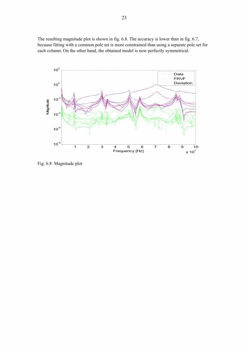
The resulting magnitude plot is shown in fig. 6.8. The accuracy is lower than in fig. 6.7, because fitting with a common pole set is more constrained than using a separate pole set for each column. On the other hand, the obtained model is now perfectly symmetrical.

Fig. 6.8 Magnitude plot

1 2 3 4 5 6 7 8 9 10x 104

10-8

10-6

10-4

10-2

100

102

Frequency [Hz]

Mag

nitu

de

DataFRVFDeviation

24

ex5.m – Transmission line modelling

The propagation function H(s) of a 5-conductor overhead line is read from file (AC line in parallel with DC line). The lossless time delay has been factored out.

One column of H is fitted with N=14 poles (7 complex pairs) directly in the phase domain

5 iterations No weighting

The result is shown in Fig. 6.9 (Magnitude function)

Fig. 6.9 Fitting a column of the propagation function. N=14 poles It is seen that the “error level” is quite “flat” as function of frequency. Fig. 6.10 shows the fitting result when introducing inverse magnitude weighting:

weight=1./abs(f);

101 102 103 104 105 10610-6

10-5

10-4

10-3

10-2

10-1

100

Frequency [Hz]

Mag

nitude

DataFRVFDeviation

Fig. 6.10 Effect of weighting with inverse of magnitude

101 102 103 104 105 10610-5

10-4

10-3

10-2

10-1

100

Frequency [Hz]

Mag

nitu

de

DataFRVFDeviation