1

Fast Space-Varying Convolution Using MatrixSource Coding with Applications to Camera Stray

Light ReductionJianing Wei,Member, IEEE,Charles A. Bouman,Fellow, IEEE,

and Jan P. Allebach,Fellow, IEEE

Abstract—Many imaging applications require the implemen-tation of space-varying convolution for accurate restoration andreconstruction of images. Here we use the term “space-varyingconvolution” to refer to linear operators whose impulse responsehas slow spatial variation. Moreover, these space-varyingcon-volution operators are often dense, so direct implementation ofthe convolution operator is typically computationally impractical.One such example is the problem of stray light reduction in digitalcameras, which requires the implementation of a dense space-varying deconvolution operator. However, other inverse problems,such as iterative tomographic reconstruction, can also depend onthe implementation of dense space-varying convolution. Whilespace-invariant convolution can be efficiently implemented withthe Fast Fourier Transform (FFT), this approach does not workfor space-varying operators. So direct convolution is often theonly option for implementing space-varying convolution.

In this paper, we develop a general approach to the efficientimplementation of space-varying convolution, and demonstrateits use in the application of stray light reduction. Our approach,which we call matrix source coding, is based on lossy sourcecoding of the dense space-varying convolution matrix. Impor-tantly, by coding the transformation matrix, we not only reducethe memory required to store it; we also dramatically reducethe computation required to implement matrix-vector products.Our algorithm is able to reduce computation by approximatelyfactoring the dense space-varying convolution operator into aproduct of sparse transforms. Experimental results show thatour method can dramatically reduce the computation requiredfor stray light reduction while maintaining high accuracy.

Index Terms—Stray light, space-varying point spread func-tion, image restoration, fast algorithm, inverse problem,digitalphotography.

I. INTRODUCTION

In many important imaging applications, it is useful tomodel the acquired data vectory as

y = Ax + w, (1)

Copyright (c) 2013 IEEE. Personal use of this material is permitted.However, permission to use this material for any other purposes must beobtained from the IEEE by sending a request to pubs-permissions@ieee.org.

This research work was done when Jianing Wei was a Ph.D. studentat the School of Electrical and Computer Engineering, Purdue University.Jianing Wei is currently with Google Inc., Mountain View, CA94043, USA.Charles A. Bouman and Jan P. Allebach are with the School of Electrical andComputer Engineering, Purdue University, West Lafayette,IN 47906, USA.Email: weijianing@gmail.com,{bouman, allebach}@purdue.edu.

This material is based upon work supported by, or in part by, the U. S. ArmyResearch Laboratory and the U. S. Army Research Office under contract/grantnumber 56541-CI, and the National Science Foundation underContract CCR-0431024.

wherex is the unknown image to be determined,A is a lineartransformation matrix, andw is some additive noise that isindependent ofx with inverse covarianceΛw. This simplelinear model can capture many important inverse problemsincluding image deblurring [1], tomographic reconstruction[2], and super-resolution [3].

There is a vast literature related to the effective solutionof inverse problems with the form of Eq. (1). Solution tothese inverse problems can be very difficult if the trans-formationsA or AtΛwA are ill conditioned. This can andoften does happen if the data is sparse, which will resultin fewer rows than columns inA, or of low quality, whichwill result in small values inΛw. In these cases, manyalgorithms have been proposed to recoverx from y. Classicalapproaches include algebraic reconstruction techniques (ART)[4]; simultaneous iterative reconstruction technique (SIRT) [5];simultaneous algebraic reconstruction technique (SART) [6];Lucy-Richardson algorithm [7]; Van Cittert’s method [1], [8];approximate [9] or true [10] maximum likelihood estimation;regularized inversion [11]; and maximum a posteriori (MAP)estimate with different priors [12], [13], [14], [15], [16], [17];Bayesian minimum mean squared error (MMSE) estimate withhigh-order Markov Random Field (MRF) prior [18]; and directdeconvolution followed by artifact removal using a machinelearning approach [19]. A common objective in all thesemethods is to balance the goal of matching the observed (butnoisy) data with the goal of producing a physically realisticimage.

While many methods exist for addressing the inverse prob-lem of Eq. (1), all these methods typically require the com-putation of matrix-vector products, such asAx, or Aty. Infact, iterative inversion methods typically require the repeatedcomputation of the matrix-vector productAtAx or AtΛwAx.If the matrix A is sparse, as is the case with a differentialoperator [20], or if it can be decomposed as a product ofsparse transformations, as is the case with the wavelet [21]or fast Fourier transform (FFT) [22], then computation ofAxis fast and tractable. For example, ifAx is space-invariantconvolution, thenA can be decomposed as the product of twoFFTs and a diagonal transform, resulting in a total computationfor the evaluation ofAx that has an order ofO(P log P ) whereP is the size ofx.

However, in many important applications,A representsspace-varying convolution where we define “space-varyingconvolution” to be a linear operator whose impulse response

2

varies slowly with position in the image. More specifically,when A represents 1D convolution, then it must have theproperty that

Aq,p = h(q − p) (2)

for some functionh(·) that represents the impulse response ofthe operator. HereAq,p represents the reponse at locationq toa stimulus at locationp. So we use the term “space-varyingconvolution” to mean thatA can be written as

Aq,p = h(q − p, p), (3)

where h(·, p) is a slowly varying function ofp. The 2Dcase is similar, withq and p representing vector indices. IfA represents space-varying convolution with a large point-spread function, then each direct evaluation of the matrix-vector productAx or Aty can require enormous computation.Even whenAtA is approximately Toeplitz, as is often the casein tomographic reconstruction [4], the matrixAtΛwA will notbe Toeplitz when the noise is space varying.

The specific application considered in this paper is thatof stray light reduction for digital photographs [23]. Straylight refers to the portion of the entering light flux that ismisdirected to undesired locations in the image plane. It issometimes referred to as lens flare or veiling glare [24]. It canbe caused by imperfections in lens elements, or reflectionsbetween optical surfaces; but in the end, it tends to reducethe contrast of images by scattering light from bright regionsof the image into dark regions. Since stray light is typicallyscattered across the imaging field, its associated point spreadfunction (PSF) typically has large support and is space-varying[23]. With this in mind, an imaging system with stray lightcan be modeled using Eq. (1) with

A = (1 − β)I + βS, (4)

whereI is the identity matrix,S is a dense matrix describingthe space-varying scattering of light across the imaging array1,andβ is a scalar constant representing the fraction of scatteredlight.

Typically the fraction of scattered light is small, and weknow that the matrixA is very well conditioned, so in contrastto many inverse problems, stray light reduction is a well-posedinverse problem, and the solution can be computed using aformula such as that proposed by Jansson and Fralinger [25]

x = (1 + β)y − βSy, (5)

wherey is the observed image, andx is the estimate of theunderlying image to be recovered.

However, even in this simple form, the computation ofEq. (5) is not practical for a modern digital camera, becausethe matrix S is both dense and lacks a Toeplitz structure.In typical stray light models, the PSF is space-varying withheavy tails, so the FFT cannot be directly used to speed upcomputation [23]. For example, if the image containsP pixels,the computation isO(P 2); so for a106 pixel image, it takes106 multiplies to compute each output pixel, resulting in a total

1Due to conservation of energy, we know that the columns ofS sum toless than 1.

of 1012 multiplies. This much computation requires hours ofprocessing time, which makes accurate stray light reductioninfeasible for implementation in low cost digital cameras.

There are several approaches in the literature to computespace-varying convolution. The overlap-add method [26], [27],[28] partitions the input space into isoplanatic patches andassumes that the PSF within each patch is spatially invariant.Then the FFT can be used to efficiently compute the result foreach patch; and they are added together. The efficient filterflow approach [29] is also based on this method. Anotherapproach is to approximate the space-varying convolutionas the weighted linear combination of a small number ofconvolutions with fixed PSF [30], [31].

In this paper, we propose a novel algorithm for fast com-putation of space-varying convolution; and we demonstrateits effectiveness for the particular application of stray lightreduction. This paper is an extension to our earlier conferencepaper [32], but it incorporates substantial new theoretical andexperimental results. Our method, which we refer to as matrixsource coding (MSC), is based on the use of lossy sourcecoding techniques to compress the dense matrixS into asparse form. Importantly, the effect of this compression isnot only to reduce the memory required for storingS, butalso to dramatically reduce the number of multiplies requiredto approximately compute the matrix-vector productSy. Ourapproach works by first decorrelating the rows and columnsof S, and then quantizing the resulting compacted matrix sothat most of its entries become zero.

Our MSC method requires both on-line and off-line compo-nents. While the on-line component is fast, it requires the pre-computation of a sparse matrix decomposition in an off-lineprocedure. We introduce a method for efficiently implementingthis off-line computation for a broad class of space-varyingkernels whose wavelet coefficients are localized in space.

In order to assess the value of our approach, we apply it tothe problem of stray light reduction for digital cameras. Usingthe stray light model of [23], we demonstrate that the MSCmethod can achieve an accuracy of 1% with approximately7 multiplies per pixel at image resolution1024 × 1024, adramatic reduction when compared to direct space-varyingconvolution. We also demonstrate the effectiveness of a prac-tical pre-computation algorithm that can be performed intime proportional to the kernel size, and show that the MSCapproach compares favorable to the overlap-add method.

In Section II we introduce the MSC method. The on-line algorithm for space-varying convolution is derived andpresented in Section II-A, and the off-line pre-computationmethod is presented in Section II-B and Section IV. Section IIIpresents the stray light application and model, and SectionVfollows with experimental results. Section VI concludes thispaper.

II. M ATRIX SOURCE CODING APPROACH TO

SPACE-VARYING CONVOLUTION

In this section, we present the matrix source coding (MSC)approach for fast space-varying convolution. The MSC ap-proach has two parts, which we will refer to as the on-line

3

and off-line computations. The on-line algorithm computesthespace-varying convolution using a product of sparse matrices.Section II-A presents the on-line algorithm along with itsassociated theory.

While the on-line computation is very fast, it depends onthe result of off-line computation, which is to pre-computea sparse version of the original space-varying convolutionmatrix. This computation is not input image-dependent, andonly depends on the PSF of the imaging system. However,naive computation of this sparse matrix can be enormouslycomputationally demanding. So in Section II-B, we introducean efficient algorithm for accurate but approximate computa-tion of the required sparse transformation for a broad classofproblems.

A. Matrix Source Coding Theory

Our goal is to speed up the computation of general matrix-vector products with the form

z = Sy, (6)

where y is the input, z is the output, andS is a denseP × P matrix without a Toeplitz structure.2 Without lossof generality, we assumey is zero mean since it is alwayspossible to subtract offy’s mean. IfS is Toeplitz, thenSy canbe efficiently computed using the fast Fourier transform (FFT)[33]. However, whenS implements space-varying convolution,then it is not Toeplitz; and the FFT cannot be used directly.

Our strategy for speeding up computation ofSy is to uselossy transform coding of the rows and columns ofS. Theresulting coded matrix then becomes sparse after quantiza-tion, and this sparsity reduces both storage and computation.However, in order to perform lossy source coding ofS, wemust first determine the relevant distortion metric.

In general, the mean squared error (MSE) is not a gooddistortion metric for codingS because it does not account forany correlation in the vectory. In order to see this, let[S]be a quantized version ofS produced by lossy coding anddecoding. Then the distortion introduced into the outputz,which we denote asδz, is given by

δz , S y − [S] y = δS y, (7)

whereδS , S−[S] is the distortion introduced intoS throughlossy coding andδz is the resulting distortion introduced intoz. Using the argument of [34], [35] and assuming thaty isindependent ofδS, then the conditional expectation of theMSE in z given δS can be written as

E[

‖δz‖2|δS]

= E[

trace{δzδzt}|δS]

= E[

trace{δSyytδSt}|δS]

= trace{δS E[

yyt|δS]

δSt}

= trace{δS Ry δSt}, (8)

where E[

‖δz‖2|δS]

means the expectation of MSE inz givenδS, andRy = E[yyt] = E [yyt|δS]. Notice that in the special

2In fact, all our results hold whenS is a non-squareP1 × P2 matrix.However, we consider the special case ofP = P1 = P2 here for notationalsimplicity. The extension to the more general case is direct.

case wheny is white, then we have thatRy = I, and

E[

‖δz‖2|δS]

= ‖δS‖2 . (9)

In other words, when the inputy is white, minimizing thesquared error distortion of the matrixS (i.e., the Frobeniusnorm) is equivalent to minimizing the expected value of thesquared error distortion forz. However, when the componentsof y are correlated, then minimum MSE coding ofS can bequite far from minimizing the MSE inz.

So with this result in mind, our objective will be to find twotransformsW1 andT that simultaneously sparsify the matrixS and whiten the random vectory. More specifically, definethe transformed matrixS as

S = W1S T−1, (10)

whereW1 is an orthonormal transform3 andT is an invertibletransform. Then the outputz can be computed as

z = W−11 S T y . (11)

So if we temporarily ignore the computational cost of thetransformsT and W1, then the computation of Eq. (11) isgreatly reduced whenS is made sparse. Furthermore, thesparsity can be increased by quantizingS. So if [S] representsthe quantized version ofS, then the approximate output canbe computed as

z = W−11 [S] Ty , (12)

wherez is the approximation ofz. If y = Ty is approximatelywhite, then MMSE quantization ofS will result in a MMSEestimatez.

So this all begs the question of what transforms can bestachieve this goal? In order to answer this question, we firstadopt the following definition.

Definition 1: We say that(W1, T ) are optimal for thetransform S and the zero-mean random input vectory, ifthe following three properties hold: a)W1 is orthonormal;b) y = Ty is white so that E[yyt] = I; and c) the matrixS = W1ST−1 is diagonal.

At this point, it is useful to make a few observations. Firstnotice that if we can find(W1, T ) that produce a diagonalmatrix S, then this is the most sparse matrix possible. In thiscase, the number of non-zero elements inS must equal therank ofS. Second, ifT whitens the random vectory, then byEq. (9) we know that minimum mean square error (MMSE)quantization ofS will result in the MMSE representation ofz.For these two reasons, we say that such a choice of(W1, T )is optimal.

In fact, such an optimal choice of(W1, T ) always exists asshown in Appendix A. In particular, define the matrix

F = SEyΛ1/2y (13)

where Ry = EyΛyEty is the eigen decomposition of the

covariance ofy, and letF = UΣV t be the singular value

3More generally, this transform can just be assumed to be orthogonal. Butfor notional simplicity we also assume it is normal, i.e. each row and columnhas a Euclidean norm of1.

4

decomposition ofF . Then the optimal choices of(W1, T ) aregiven by

T = V t Λ−1/2y Et

y , (14)

andW1 = U t . (15)

Intuitively, the optimal transformW1 decorrelates the rowsof F and the optimal transformT−1 decorrelates the columnsof S. When this is done, the transformed matrix of Eq. (10)is then diagonal withS = Σ. In fact, when the eigen valuesΛy and singular valuesΣ are unique, then these transformsmust also be unique up to permutations and scaling by±1(see Appendix A).

Unfortunately, the optimal choice of(W1, T ) is typicallynot practical. This is because to achieve this ideal sparsity,the transformsW1 and T must typically be dense matrices.However, if the transformsT and W1 are dense, then theapplication of these decorrelating transforms requires asmuchcomputation as the original multiplication byS. This would,of course, defeat the purpose of the sparsification ofS.

So our practical objective is to find computationally efficienttransformations,(W1, T ), that approximately whiteny, andapproximately decorrelate the rows ofF and the columns ofS. Intuitively, the transformsW1 andT concentrate the energyin the rows and columns of the matrixS in much the sameway that transform coding concentrates the energy in a signal.

To achieve this practical objective, we will use a wavelettransform to approximately decorrelate the vectory, the rowsof F , and the columns ofS. In our applications,y is animage which can be modeled as a stationary random process.In this case, it is well-known that the wavelet transform isa reasonable choice for the decorrelation ofy because itis known to be an approximation to the Karhunen-Loevetransform for stationary sources [36], and it is commonlyused as a decorrelating transform for various source codingapplications [37].

Using this strategy, we form the matrixT by a wavelettransform followed by gain factors designed to normalizethe variance of wavelet coefficients. This combination ofdecorrelation and scaling whitens or spheres the vectory.Specifically, we choose

T = Λ−1/2w W2 , (16)

whereW2 is an orthonormal wavelet transform andΛ−1/2w is

a diagonal matrix of gain factors so that

Λw = diag(

W2RyW t2

)

, (17)

whereRy = E[yyt] is the covariance ofy.At the same time, notice that the transformT−1 =

W−12 Λ

1/2w approximately decorrelates the columns ofS when

S represents space-varying convolution. This is true becauseif S is a slowly space-varying operator, then the covariancematrix of the columns given byRc = StS is approximatelyToeplitz. Again, it is well-known that the if covarianceRc isToeplitz, then this corresponds to the covariance of a wide-sense stationary random process, and the wavelet transformis a good approximation to the diagonalizing Karhunen-Loevetransform [36].

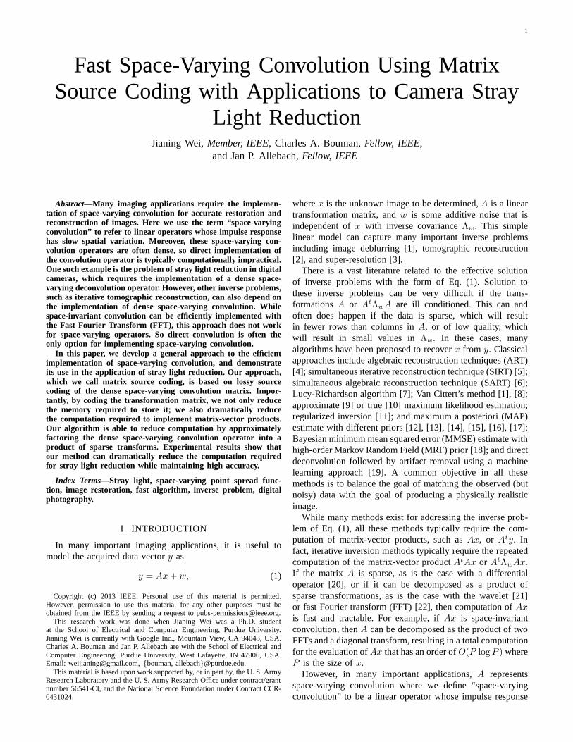
Fig. 1. Block diagram of on-line computation of matrix source coding.

With this choice forT of Eq. (16), then the matrixF isgiven by

F = SW t2Λ1/2

w . (18)

Again, the matrixRr = FF t that represents the covariance ofthe rows ofF is approximately Toeplitz, so the rows ofF canbe approximately decorrelated with an orthonormal wavelettransformW1.

To summarize, Fig. 1 illustrates a block diagram of the on-line computation we will use for matrix source coding. Inparticular, the approximate output is computed as

z = W t1 [S]Λ

−1/2W W2y, (19)

where[S] is a quantized version of the transformed matrix

S = W1SW−12 Λ1/2

w . (20)

First, the input datay is transformed and scaled. Then itis multiplied by a sparse matrix[S]. Then a second inversewavelet transform is applied to compute the approximate resultz. The accuracy of the approximation is determined by thedegree of quantization applied toS, with coarser quantizationresulting in lower accuracy. So if little or no quantizationis used, then the computation can be arbitrarily close toexact, but at the cost of less sparsity inS and thereforemore computation and storage. In this way, matrix sourcecoding allows for a continuous trade-off between accuracy andcomputation/storage in much the same way that signal sourcecoding allows for a rate-distortion trade-off in applicationssuch as image and video coding.

Finally, as a practical matter, the diagonal matrixΛw can beeasily estimated from training images. In fact, we will assumethat the gain factors for each subband are constant since thewavelet coefficients in the same subband typically have thesame variance [1]. So to estimateΛw, we take the wavelettransformW2 of the training images, compute the varianceof the wavelet coefficients in each subband, and average overall images to obtain an estimate of the gain factors for eachsubband.

B. Efficient Off-Line Computation for Matrix Source Coding

In order to implement the fast space-varying convolutionmethod described by Eq. (19), it is first necessary to computethe source coded matrix[S]. We will refer to the computationof [S] as the off-line portion of the computation. Once thesparse matrix[S] is available, then the space-varying convo-lution may be efficiently computed using on-line computationshown in Eq. (19).

However, even though the computation of[S] is performedoff-line, exact evaluation of this sparse matrix is still too largefor practical problems. For example, if the image contains16million pixels (i.e,224 pixels) and each matrix entry is stored

5

as a4-byte integer, then the temporary storage ofS requiresapproximately4 × 248 bytes or equivalently one petabyte ofstorage. Of course, this much storage exceeds the capacity ofmost modern computers. So, the following section describesan efficient approach to compute[S] which eliminates the needfor any such temporary storage.

In our implementation, we use the Haar wavelet transform[21] for both W1 andW2. The Haar wavelet transform is anorthonormal transform, so we have that

S = W1ST−1

= W1SW t2Λ1/2

w . (21)

Therefore, direct implementation of this off-line computationconsists of a wavelet transformW2 along the rows ofS,scaling of the matrix entries, and a wavelet transformW1 alongthe columns. Unfortunately, the computational complexityofthese two operations isO(P 2), whereP is the number ofpixels in the image, because the operation requires that eachentry ofS be touched. This computation can take a tremendousamount of time for high resolution images. Therefore, weaim at reducing the computational complexity to be linearlyproportional toP and eliminating the need to store the entirematrix S. In order to achieve this goal, we will use a twostage quantization procedure combined with a recursive top-down algorithm for computing the Haar wavelet transformcoefficients.

The first stage of this procedure is to zero out the entriesin SW t

2Λ1/2w whose magnitudes are less than a specified

threshold. We useQt(SW t2Λ

1/2w ) to describe this thresholding

stage, where for a scalarx

Qt(x) =

{

x for |x| > t0 otherwise

. (22)

The resulting matrixQt(SW t2Λ

1/2w ) is already quite sparse,

thus there is no need to store the entire dense matrix. Thevalue of the thresholdt is chosen to achieve some targetsparsity,N << P , whereN is the average number of non-zero elements per row of the matrixQt(SW t

2Λ1/2w ).

The second stage of this procedure is to compute the wavelettransformW1 over the columns of this already sparse matrix.Taking advantage of the sparsity resulting from the first stage,then the computation of the wavelet transform in the secondstage is reduced fromO(P 2) to O(NP ). In summary, thistwo stage procedure is expressed mathematically as

[S] ≈ [W1Qt(SW t2Λ1/2

w )]. (23)

In practice,N should be chosen to be sufficiently large sothat the accuracy-computation trade-off of the matrix-sourcecoding is not impaired, but sufficiently small that the memoryrequirements for temporary storage are not excessive. In theexperimental results section, we illustrate this trade-off.

However, there is still a problem as to how to efficientlycomputeQt(SW t

2Λ1/2w ). SinceS is dense, direct evaluation

of this expression requiresO(P 2) operations. However, afterthresholding, most values inQt(SW t

2Λ1/2w ) are zero, so we

can dramatically reduce computation by first identifying theregions where non-zero values are likely to occur. We refer

to these non-zero values as significant wavelet coefficients.As mentioned before, we useN to denote the number ofsignificant wavelet coefficients per row. Once we can predictthe location of the significant wavelet coefficients, we can use arecursive top-down approach to compute them without havingto do the full wavelet transform for each row ofS. We willdiscuss how to predict the location of the significant waveletcoefficients in constant time in Sec. IV.

Next, we describe our algorithm for computing the signif-icant wavelet coefficients once their location is known. Ourstrategy is to first compute the approximation coefficients thatare necessary to compute the significant wavelet coefficientsusing a recursive top-down approach. Then significant detailcoefficients can be computed from the approximation coef-ficients at finer resolutions. Our approach is able to achieveO(N) computational complexity for computing the significantHaar wavelet coefficients per row, which leads to a totalcomplexity ofO(NP ) for computingQt(SW t

2Λ1/2w ).

We usef(q, k, i, j) to represent the approximation coeffi-cient for rowq of matrixS at location(i, j) and levelk, wherelarger values ofk correspond to coarser scales, andf(q, 0, i, j)corresponds to the full resolution image for rowq. We usegh(q, k, i, j), gv(q, k, i, j), and gd(q, k, i, j) to represent thedetail coefficients in horizontal, vertical and diagonal bands,respectively. We can then computef(q, k, i, j) as the averageof its corresponding 4 higher resolution neighbors:

f(q, k, i, j) =1

2(f(q, k − 1, 2i, 2j) + f(q, k − 1, 2i + 1, 2j)

+f(q, k − 1, 2i, 2j + 1)

+f(q, k − 1, 2i + 1, 2j + 1)). (24)

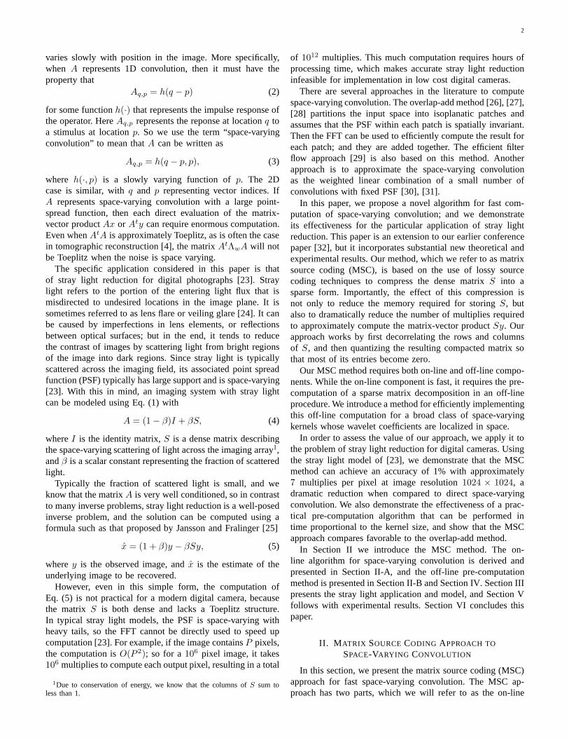
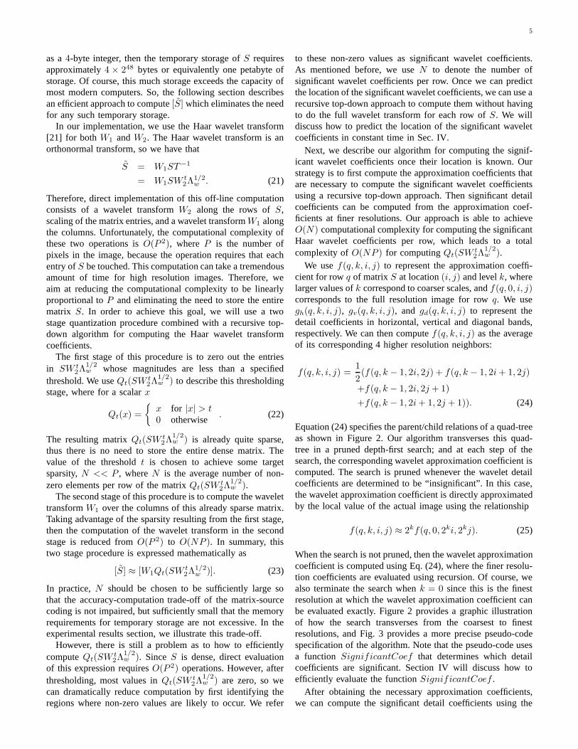
Equation (24) specifies the parent/child relations of a quad-treeas shown in Figure 2. Our algorithm transverses this quad-tree in a pruned depth-first search; and at each step of thesearch, the corresponding wavelet approximation coefficient iscomputed. The search is pruned whenever the wavelet detailcoefficients are determined to be “insignificant”. In this case,the wavelet approximation coefficient is directly approximatedby the local value of the actual image using the relationship

f(q, k, i, j) ≈ 2kf(q, 0, 2ki, 2kj). (25)

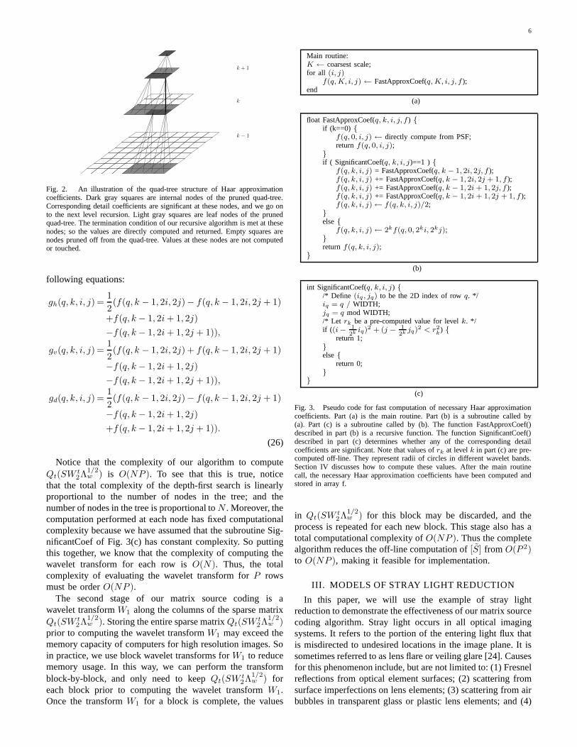
When the search is not pruned, then the wavelet approximationcoefficient is computed using Eq. (24), where the finer resolu-tion coefficients are evaluated using recursion. Of course,wealso terminate the search whenk = 0 since this is the finestresolution at which the wavelet approximation coefficient canbe evaluated exactly. Figure 2 provides a graphic illustrationof how the search transverses from the coarsest to finestresolutions, and Fig. 3 provides a more precise pseudo-codespecification of the algorithm. Note that the pseudo-code usesa function SignificantCoef that determines which detailcoefficients are significant. Section IV will discuss how toefficiently evaluate the functionSignificantCoef .

After obtaining the necessary approximation coefficients,we can compute the significant detail coefficients using the

6

k + 1

k

k − 1

Fig. 2. An illustration of the quad-tree structure of Haar approximationcoefficients. Dark gray squares are internal nodes of the pruned quad-tree.Corresponding detail coefficients are significant at these nodes, and we go onto the next level recursion. Light gray squares are leaf nodes of the prunedquad-tree. The termination condition of our recursive algorithm is met at thesenodes; so the values are directly computed and returned. Empty squares arenodes pruned off from the quad-tree. Values at these nodes are not computedor touched.

following equations:

gh(q, k, i, j) =1

2(f(q, k − 1, 2i, 2j)− f(q, k − 1, 2i, 2j + 1)

+f(q, k − 1, 2i + 1, 2j)

−f(q, k − 1, 2i + 1, 2j + 1)),

gv(q, k, i, j) =1

2(f(q, k − 1, 2i, 2j) + f(q, k − 1, 2i, 2j + 1)

−f(q, k − 1, 2i + 1, 2j)

−f(q, k − 1, 2i + 1, 2j + 1)),

gd(q, k, i, j) =1

2(f(q, k − 1, 2i, 2j)− f(q, k − 1, 2i, 2j + 1)

−f(q, k − 1, 2i + 1, 2j)

+f(q, k − 1, 2i + 1, 2j + 1)).

(26)

Notice that the complexity of our algorithm to computeQt(SW t

2Λ1/2w ) is O(NP ). To see that this is true, notice

that the total complexity of the depth-first search is linearlyproportional to the number of nodes in the tree; and thenumber of nodes in the tree is proportional toN . Moreover, thecomputation performed at each node has fixed computationalcomplexity because we have assumed that the subroutine Sig-nificantCoef of Fig. 3(c) has constant complexity. So puttingthis together, we know that the complexity of computing thewavelet transform for each row isO(N). Thus, the totalcomplexity of evaluating the wavelet transform forP rowsmust be orderO(NP ).

The second stage of our matrix source coding is awavelet transformW1 along the columns of the sparse matrixQt(SW t

2Λ1/2w ). Storing the entire sparse matrixQt(SW t

2Λ1/2w )

prior to computing the wavelet transformW1 may exceed thememory capacity of computers for high resolution images. Soin practice, we use block wavelet transforms forW1 to reducememory usage. In this way, we can perform the transformblock-by-block, and only need to keepQt(SW t

2Λ1/2w ) for

each block prior to computing the wavelet transformW1.Once the transformW1 for a block is complete, the values

Main routine:K ← coarsest scale;for all (i, j)

f(q, K, i, j) ← FastApproxCoef(q, K, i, j, f );end

(a)

float FastApproxCoef(q, k, i, j, f ) {if (k==0) {

f(q, 0, i, j) ← directly compute from PSF;returnf(q, 0, i, j);

}if ( SignificantCoef(q, k, i, j)==1 ) {

f(q, k, i, j) = FastApproxCoef(q, k − 1, 2i, 2j, f );f(q, k, i, j) += FastApproxCoef(q, k − 1, 2i, 2j + 1, f );f(q, k, i, j) += FastApproxCoef(q, k − 1, 2i + 1, 2j, f );f(q, k, i, j) += FastApproxCoef(q, k − 1, 2i + 1, 2j + 1, f );f(q, k, i, j)← f(q, k, i, j)/2;

}else{

f(q, k, i, j)← 2kf(q, 0, 2ki, 2kj);}returnf(q, k, i, j);

}

(b)

int SignificantCoef(q, k, i, j) {/* Define (iq , jq) to be the 2D index of rowq. */iq = q / WIDTH;jq = q mod WIDTH;/* Let rk be a pre-computed value for levelk. */if ((i− 1

2k iq)2 + (j − 1

2k jq)2 < r2

k) {

return 1;}else{

return 0;}

}

(c)

Fig. 3. Pseudo code for fast computation of necessary Haar approximationcoefficients. Part (a) is the main routine. Part (b) is a subroutine called by(a). Part (c) is a subroutine called by (b). The function FastApproxCoef()described in part (b) is a recursive function. The function SignificantCoef()described in part (c) determines whether any of the corresponding detailcoefficients are significant. Note that values ofrk at levelk in part (c) are pre-computed off-line. They represent radii of circles in different wavelet bands.Section IV discusses how to compute these values. After the main routinecall, the necessary Haar approximation coefficients have been computed andstored in array f.

in Qt(SW t2Λ

1/2w ) for this block may be discarded, and the

process is repeated for each new block. This stage also has atotal computational complexity ofO(NP ). Thus the completealgorithm reduces the off-line computation of[S] from O(P 2)to O(NP ), making it feasible for implementation.

III. MODELS OF STRAY LIGHT REDUCTION

In this paper, we will use the example of stray lightreduction to demonstrate the effectiveness of our matrix sourcecoding algorithm. Stray light occurs in all optical imagingsystems. It refers to the portion of the entering light flux thatis misdirected to undesired locations in the image plane. Itissometimes referred to as lens flare or veiling glare [24]. Causesfor this phenomenon include, but are not limited to: (1) Fresnelreflections from optical element surfaces; (2) scattering fromsurface imperfections on lens elements; (3) scattering from airbubbles in transparent glass or plastic lens elements; and (4)

7

a (mm−1) b (mm−1) α c (mm)PSF parameter set 1−1.65× 10−4 −8.35× 10−4 1.21 0.015PSF parameter set 2 4× 10−3 0 1.15 0.02

TABLE ITWO SETS OFPSFPARAMETERS

scattering from dust or other particles. Images contaminatedby stray light suffer from reduced contrast and saturation.

We reduce the stray light by first formulating a PSF modelof the imaging system and then inverting the model. Thismethod is also used in previous work [23], [38], [39], [32].The PSF model for a stray light contaminated optical imagingsystem is formulated as

y = ((1 − β)I + βS)x, (27)

whereI is an identity matrix,S accounts for stray light dueto scattering and undesired reflections, andβ represents theweight factor of the stray light. The entries ofS are describedby

Sq,p = s(iq, jq; ip, jp), (28)

where (iq, jq) and (ip, jp) are the 2D indices correspondingto q andp respectively, ands(iq, jq; ip, jp) is the value of thestray light PSF at(iq, jq) due to a point source located at(ip, jp). We follow [23], [38], [39], [40] and model the straylight PSF as:

s(iq, jq; ip, jp)=1

γ×

1(

1 + 1i2p+j2

p

(

(iqip+jqjp−i2p−j2p)2

(c+a(i2p+j2p))2 +

(−iqjp+jqip)2

(c+b(i2p+j2p))2

))α ,

(29)

where γ is a normalizing constant that makes∫

iq

∫

jqs(iq, jq; ip, jp)diqdjq = 1. An analytic expression

for γ is γ = πα−1 (c + a(i2p + j2

p))(c + b(i2p + j2p)). Figure 4

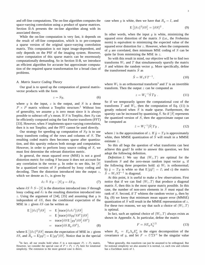
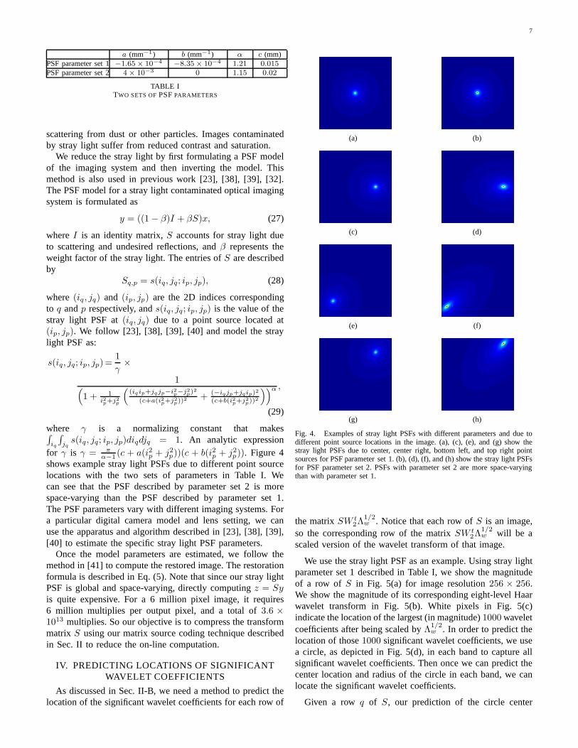
shows example stray light PSFs due to different point sourcelocations with the two sets of parameters in Table I. Wecan see that the PSF described by parameter set 2 is morespace-varying than the PSF described by parameter set 1.The PSF parameters vary with different imaging systems. Fora particular digital camera model and lens setting, we canuse the apparatus and algorithm described in [23], [38], [39],[40] to estimate the specific stray light PSF parameters.

Once the model parameters are estimated, we follow themethod in [41] to compute the restored image. The restorationformula is described in Eq. (5). Note that since our stray lightPSF is global and space-varying, directly computingz = Syis quite expensive. For a 6 million pixel image, it requires6 million multiplies per output pixel, and a total of3.6 ×1013 multiplies. So our objective is to compress the transformmatrix S using our matrix source coding technique describedin Sec. II to reduce the on-line computation.

IV. PREDICTING LOCATIONS OF SIGNIFICANTWAVELET COEFFICIENTS

As discussed in Sec. II-B, we need a method to predict thelocation of the significant wavelet coefficients for each rowof

(a) (b)

(c) (d)

(e) (f)

(g) (h)

Fig. 4. Examples of stray light PSFs with different parameters and due todifferent point source locations in the image. (a), (c), (e), and (g) show thestray light PSFs due to center, center right, bottom left, and top right pointsources for PSF parameter set 1. (b), (d), (f), and (h) show the stray light PSFsfor PSF parameter set 2. PSFs with parameter set 2 are more space-varyingthan with parameter set 1.

the matrixSW t2Λ

1/2w . Notice that each row ofS is an image,

so the corresponding row of the matrixSW t2Λ

1/2w will be a

scaled version of the wavelet transform of that image.

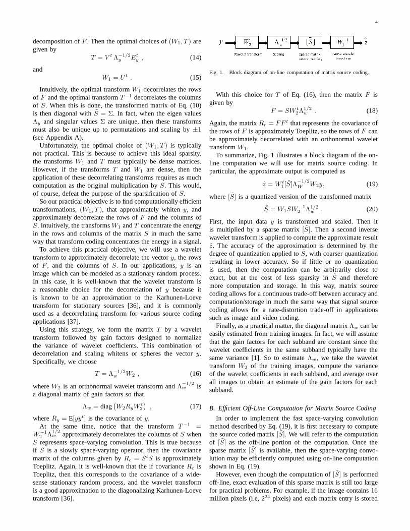
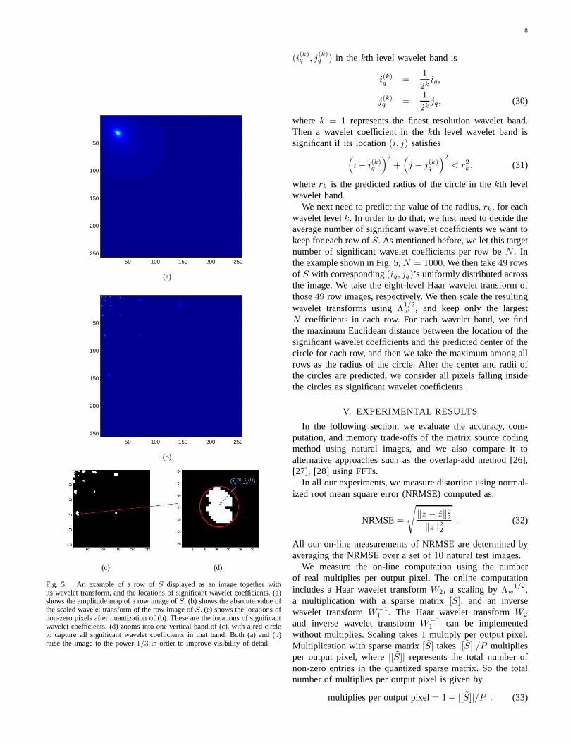
We use the stray light PSF as an example. Using stray lightparameter set 1 described in Table I, we show the magnitudeof a row of S in Fig. 5(a) for image resolution256 × 256.We show the magnitude of its corresponding eight-level Haarwavelet transform in Fig. 5(b). White pixels in Fig. 5(c)indicate the location of the largest (in magnitude)1000 waveletcoefficients after being scaled byΛ1/2

w . In order to predict thelocation of those1000 significant wavelet coefficients, we usea circle, as depicted in Fig. 5(d), in each band to capture allsignificant wavelet coefficients. Then once we can predict thecenter location and radius of the circle in each band, we canlocate the significant wavelet coefficients.

Given a row q of S, our prediction of the circle center

8

50 100 150 200 250

50

100

150

200

250

(a)

50 100 150 200 250

50

100

150

200

250

(b)

(c) (d)

Fig. 5. An example of a row ofS displayed as an image together withits wavelet transform, and the locations of significant wavelet coefficients. (a)shows the amplitude map of a row image ofS. (b) shows the absolute value ofthe scaled wavelet transform of the row image ofS. (c) shows the locations ofnon-zero pixels after quantization of (b). These are the locations of significantwavelet coefficients. (d) zooms into one vertical band of (c), with a red circleto capture all significant wavelet coefficients in that band.Both (a) and (b)raise the image to the power1/3 in order to improve visibility of detail.

(i(k)q , j

(k)q ) in the kth level wavelet band is

i(k)q =

1

2kiq,

j(k)q =

1

2kjq, (30)

where k = 1 represents the finest resolution wavelet band.Then a wavelet coefficient in thekth level wavelet band issignificant if its location(i, j) satisfies

(

i − i(k)q

)2

+(

j − j(k)q

)2

< r2k, (31)

whererk is the predicted radius of the circle in thekth levelwavelet band.

We next need to predict the value of the radius,rk, for eachwavelet levelk. In order to do that, we first need to decide theaverage number of significant wavelet coefficients we want tokeep for each row ofS. As mentioned before, we let this targetnumber of significant wavelet coefficients per row beN . Inthe example shown in Fig. 5,N = 1000. We then take49 rowsof S with corresponding(iq, jq)’s uniformly distributed acrossthe image. We take the eight-level Haar wavelet transform ofthose49 row images, respectively. We then scale the resultingwavelet transforms usingΛ1/2

w , and keep only the largestN coefficients in each row. For each wavelet band, we findthe maximum Euclidean distance between the location of thesignificant wavelet coefficients and the predicted center ofthecircle for each row, and then we take the maximum among allrows as the radius of the circle. After the center and radii ofthe circles are predicted, we consider all pixels falling insidethe circles as significant wavelet coefficients.

V. EXPERIMENTAL RESULTS

In the following section, we evaluate the accuracy, com-putation, and memory trade-offs of the matrix source codingmethod using natural images, and we also compare it toalternative approaches such as the overlap-add method [26],[27], [28] using FFTs.

In all our experiments, we measure distortion using normal-ized root mean square error (NRMSE) computed as:

NRMSE=

√

‖z − z‖22

‖z‖22

. (32)

All our on-line measurements of NRMSE are determined byaveraging the NRMSE over a set of10 natural test images.

We measure the on-line computation using the numberof real multiplies per output pixel. The online computationincludes a Haar wavelet transformW2, a scaling byΛ−1/2

w ,a multiplication with a sparse matrix[S], and an inversewavelet transformW−1

1 . The Haar wavelet transformW2

and inverse wavelet transformW−11 can be implemented

without multiplies. Scaling takes1 multiply per output pixel.Multiplication with sparse matrix[S] takes|[S]|/P multipliesper output pixel, where|[S]| represents the total number ofnon-zero entries in the quantized sparse matrix. So the totalnumber of multiplies per output pixel is given by

multiplies per output pixel= 1 + |[S]|/P . (33)

9

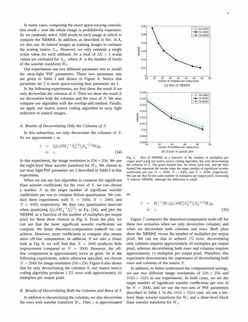
In many cases, computing the exact space-varying convolu-tion resultz over the whole image is prohibitively expensive.So we randomly select1000 pixels in each image at which tocompute the NRMSE. In addition, as described in Sec. II-A,we also use30 natural images as training images to estimatethe scaling matrixΛw. However, we only estimate a singlescalar value for each subband. So a total of3K + 1 scalarvalues are estimated forΛw, whereK is the number of levelsof the wavelet transformW2.

Our experiments use two different parameter sets to modelthe stray-light PSF parameters. These two parameter setsare given in Table I and shown in Figure 4. Notice thatparameter set 2 is more space-varying than parameter set 1.

In the following experiments, we first show the result if weonly decorrelate the columns ofS. Then we show the result ifwe decorrelate both the columns and the rows ofS. We alsocompare our algorithm with the overlap-add method. Finally,we apply our matrix source coding algorithm to stray lightreduction in natural images.

A. Results of Decorrelating Only the Columns ofS

In this subsection, we only decorrelate the columns ofS.So we approximatez as

z = [Qt(SW−12 Λ1/2

w )]Λ−1/2w W2y,

≈ z. (34)

In this experiment, the image resolution is256× 256. We usethe eight-level Haar wavelet transform forW2. We choose touse stray light PSF parameter set 1 described in Table I in thisexperiment.

When we use our fast algorithm to compute the significantHaar wavelet coefficients for the rows ofS, we can choosea numberN as the target number of significant waveletcoefficients per row to compute before quantization. We con-duct three experiments withN = 1000, N = 2000, andN = 4000, respectively. We then vary quantization intervalswhen quantizingQt(SW−1

2 Λ1/2w ) in Eq. (34), and plot the

NRMSE as a function of the number of multiplies per outputpixel for these three choices in Fig. 6. From the plot, wecan see that the more significant wavelet coefficients wecompute, the better distortion-computation tradeoff we canachieve. However, more coefficients to compute also meansmore off-line computation. In addition, if we take a closerlook at Fig. 6, we will find thatN = 4000 produces littleimprovement compared toN = 2000. However, the off-line computation is approximately twice as great. So in thefollowing experiments, unless otherwise specified, we chooseN = 2000 for image resolution256×256. Figure 6 also showsthat by only decorrelating the columnsS, our matrix sourcecoding algorithm produces1.2% error with approximately44multiplies per output pixel.

B. Results of Decorrelating Both the Columns and Rows ofS

In addition to decorrelating the columns, we also decorrelatethe rows with wavelet transformW1. Thenz is approximated

15 20 25 30 35 40 45 50 550

0.01

0.02

0.03

0.04

0.05

0.06

number of multiplies per output pixel

NR

MS

E

N=1000N=2000N=4000

(a) Plot of NRMSE

40 42 44 46 48 500.008

0.009

0.01

0.011

0.012

0.013

0.014

0.015

0.016

number of multiplies per output pixel

NR

MS

E

N=1000N=2000N=4000

(b) Zoom in partial plot

Fig. 6. Plot of NRMSE as a function of the number of multipliesperoutput pixel using our matrix source coding algorithm, but only decorrelatingthe columns ofS. The green dashed line, the black solid line, and the bluedashed line represent the results when the target number of significant waveletcoefficients per rowN = 1000, N = 2000, and N = 4000, respectively.We can see that for the same number of multiplies per output pixel, increasingN reduces NRMSE, although the difference is small.

as

z = W−11 [W1Qt(SW t

2Λ1/2w )]Λ−1/2

w W2y,

≈ z. (35)

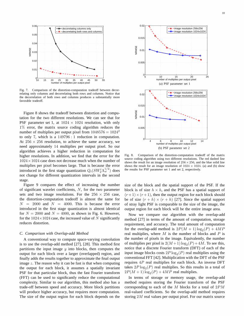
Figure 7 compares the distortion-computation trade-off forthese two scenarios when we only decorrelate columns; andwhen we decorrelate both columns and rows. Both plotsshow the NRMSE versus the number of multiplies per outputpixel. We can see that to achieve1% error, decorrelatingonly columns requires approximately48 multiplies per outputpixel, whereas decorrelating both rows and columns requiresapproximately14 multiplies per output pixel. Therefore, thisexperiment demonstrates the importance of decorrelating bothrows and columns of the matrixS.

In addition, to better understand the computational savings,we use two different image resolutions of256 × 256 and1024 × 1024 in our experiments. In both cases, we set thetarget number of significant wavelet coefficients per row tobe N = 2000, and we use the two sets of PSF parametersdescribed in Table I. In the1024 × 1024 case, we use a ten-level Haar wavelet transform forW2 and a three-level blockHaar wavelet transform forW1.

10

10 15 20 25 30 35 40 45 50 550

0.01

0.02

0.03

0.04

0.05

0.06

number of multiplies per output pixel

NR

MS

E

decorrelating columns onlydecorrelating both rows and columns

Fig. 7. Comparison of the distortion-computation tradeoffbetween decor-relating only columns and decorrelating both rows and columns. Notice thatthe decorrelation of both rows and columns produces a substantially morefavorable tradeoff.

Figure 8 shows the tradeoff between distortion and compu-tation for the two different resolutions. We can see that forPSF parameter set 1, at1024 × 1024 resolution, with only1% error, the matrix source coding algorithm reduces thenumber of multiplies per output pixel from1048576 = 10242

to only 7, which is a 149796 : 1 reduction in computation.At 256 × 256 resolution, to achieve the same accuracy, weneed approximately14 multiplies per output pixel. So ouralgorithm achieves a higher reduction in computation forhigher resolutions. In addition, we find that the error for the1024×1024 case does not decrease much when the number ofmultiplies per pixel becomes large. That is because the errorintroduced in the first stage quantizationQt(SW t

2Λ1/2w ) does

not change for different quantization intervals in the secondstage.

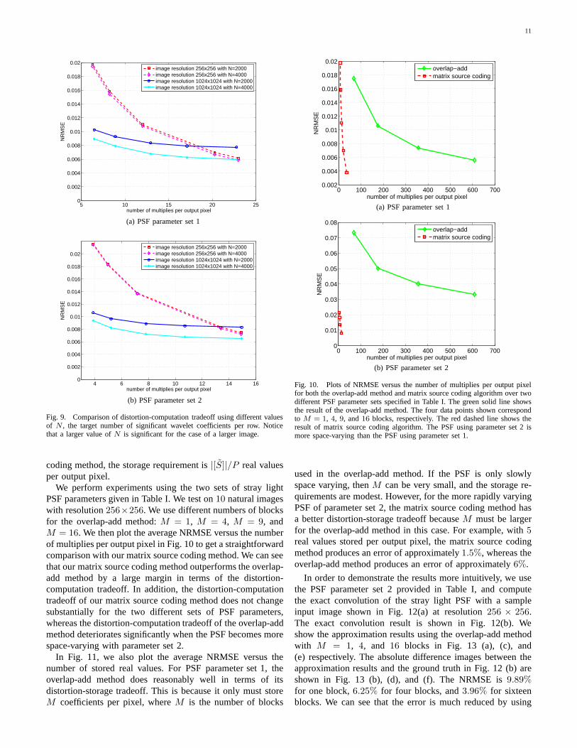
Figure 9 compares the effect of increasing the numberof significant wavelet coefficients,N , for the two parametersets and two image resolutions. For the256 × 256 case,the distortion-computation tradeoff is almost the same forN = 2000 and N = 4000. This is because the errorintroduced in the first stage quantization is almost identicalfor N = 2000 andN = 4000, as shown in Fig. 6. However,for the1024×1024 case, the increased value ofN significantlyreduces distortion.

C. Comparison with Overlap-add Method

A conventional way to compute space-varying convolutionis to use the overlap-add method [27], [28]. This method firstpartitions the input imagey into blocks, then computes theoutput for each block over a larger (overlapped) region, andfinally adds the results together to approximate the final outputimagez. The reason why it can be fast is that when computingthe output for each block, it assumes a spatially invariantPSF for that particular block, thus the fast Fourier transform(FFT) can be used to significantly reduce the computationalcomplexity. Similar to our algorithm, this method also has atrade-off between speed and accuracy. More block partitionswill produce higher accuracy, but requires more computation.The size of the output region for each block depends on the

5 10 15 20 250

0.005

0.01

0.015

0.02

number of multiplies per output pixel

NR

MS

E

image resolution 256x256image resolution 1024x1024

(a) PSF parameter set 1

4 6 8 10 12 140

0.005

0.01

0.015

0.02

number of multiplies per output pixel

NR

MS

E

image resolution 256x256image resolution 1024x1024

(b) PSF parameter set 2

Fig. 8. Comparison of the distortion-computation tradeoffof the matrixsource coding algorithm using two different resolutions. The red dashed lineshows the result for an image resolution of256×256, and the blue solid lineshows the result for an image resolution of1024 × 1024. (a) and (b) showthe results for PSF parameter set 1 and set 2, respectively.

size of the block and the spatial support of the PSF. If theblock is of sizeh × h, and the PSF has a spatial support of(r+1)× (r+1), then the output region for each block shouldbe of size(r + h) × (r + h) [27]. Since the spatial supportof stray light PSF is comparable to the size of the image, theoutput region for each block will be the entire image area.

Now we compare our algorithm with the overlap-addmethod [27] in terms of the amount of computation, storagerequirement, and accuracy. The total amount of computationfor the overlap-add method is2P (M + 1) log2(P ) + 4MPreal multiplies, whereM is the number of blocks andP isthe number of pixels in the image. Equivalently, the numberof multiplies per pixel is2(M +1) log2(P )+4M . To see this,notice that a discrete Fourier transform (DFT) of each of theinput image blocks costs2P log2(P ) real multiplies using theconventional FFT [42]. Multiplication with the DFT of the PSFrequires4P real multiplies for each block. An inverse DFTtakes2P log2(P ) real multiplies. So this results in a total of2P (M + 1) log2(P ) + 4MP real multiplies.

In terms of storage or memory usage, the overlap-addmethod requires storing the Fourier transform of the PSFcorresponding to each of theM blocks for a total of2PMreal-valued coefficients. So the overlap-add method requiresstoring2M real values per output pixel. For our matrix source

11

5 10 15 20 250

0.002

0.004

0.006

0.008

0.01

0.012

0.014

0.016

0.018

0.02

number of multiplies per output pixel

NR

MS

E

image resolution 256x256 with N=2000image resolution 256x256 with N=4000image resolution 1024x1024 with N=2000image resolution 1024x1024 with N=4000

(a) PSF parameter set 1

4 6 8 10 12 14 160

0.002

0.004

0.006

0.008

0.01

0.012

0.014

0.016

0.018

0.02

number of multiplies per output pixel

NR

MS

E

image resolution 256x256 with N=2000image resolution 256x256 with N=4000image resolution 1024x1024 with N=2000image resolution 1024x1024 with N=4000

(b) PSF parameter set 2

Fig. 9. Comparison of distortion-computation tradeoff using different valuesof N , the target number of significant wavelet coefficients per row. Noticethat a larger value ofN is significant for the case of a larger image.

coding method, the storage requirement is|[S]|/P real valuesper output pixel.

We perform experiments using the two sets of stray lightPSF parameters given in Table I. We test on10 natural imageswith resolution256×256. We use different numbers of blocksfor the overlap-add method:M = 1, M = 4, M = 9, andM = 16. We then plot the average NRMSE versus the numberof multiplies per output pixel in Fig. 10 to get a straightforwardcomparison with our matrix source coding method. We can seethat our matrix source coding method outperforms the overlap-add method by a large margin in terms of the distortion-computation tradeoff. In addition, the distortion-computationtradeoff of our matrix source coding method does not changesubstantially for the two different sets of PSF parameters,whereas the distortion-computation tradeoff of the overlap-addmethod deteriorates significantly when the PSF becomes morespace-varying with parameter set 2.

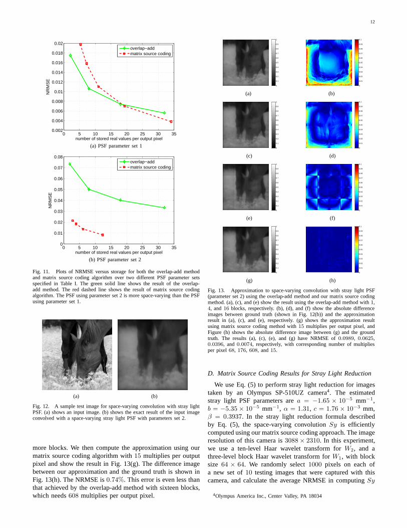
In Fig. 11, we also plot the average NRMSE versus thenumber of stored real values. For PSF parameter set 1, theoverlap-add method does reasonably well in terms of itsdistortion-storage tradeoff. This is because it only must storeM coefficients per pixel, whereM is the number of blocks

0 100 200 300 400 500 600 7000.002

0.004

0.006

0.008

0.01

0.012

0.014

0.016

0.018

0.02

number of multiplies per output pixel

NR

MS

E

overlap−addmatrix source coding

(a) PSF parameter set 1

0 100 200 300 400 500 600 7000

0.01

0.02

0.03

0.04

0.05

0.06

0.07

0.08

number of multiplies per output pixel

NR

MS

E

overlap−addmatrix source coding

(b) PSF parameter set 2

Fig. 10. Plots of NRMSE versus the number of multiplies per output pixelfor both the overlap-add method and matrix source coding algorithm over twodifferent PSF parameter sets specified in Table I. The green solid line showsthe result of the overlap-add method. The four data points shown correspondto M = 1, 4, 9, and16 blocks, respectively. The red dashed line shows theresult of matrix source coding algorithm. The PSF using parameter set 2 ismore space-varying than the PSF using parameter set 1.

used in the overlap-add method. If the PSF is only slowlyspace varying, thenM can be very small, and the storage re-quirements are modest. However, for the more rapidly varyingPSF of parameter set 2, the matrix source coding method hasa better distortion-storage tradeoff becauseM must be largerfor the overlap-add method in this case. For example, with5real values stored per output pixel, the matrix source codingmethod produces an error of approximately1.5%, whereas theoverlap-add method produces an error of approximately6%.

In order to demonstrate the results more intuitively, we usethe PSF parameter set 2 provided in Table I, and computethe exact convolution of the stray light PSF with a sampleinput image shown in Fig. 12(a) at resolution256 × 256.The exact convolution result is shown in Fig. 12(b). Weshow the approximation results using the overlap-add methodwith M = 1, 4, and 16 blocks in Fig. 13 (a), (c), and(e) respectively. The absolute difference images between theapproximation results and the ground truth in Fig. 12 (b) areshown in Fig. 13 (b), (d), and (f). The NRMSE is9.89%for one block,6.25% for four blocks, and3.96% for sixteenblocks. We can see that the error is much reduced by using

12

0 5 10 15 20 25 30 350.002

0.004

0.006

0.008

0.01

0.012

0.014

0.016

0.018

0.02

number of stored real values per output pixel

NR

MS

E

overlap−addmatrix source coding

(a) PSF parameter set 1

0 5 10 15 20 25 30 350

0.01

0.02

0.03

0.04

0.05

0.06

0.07

0.08

number of stored real values per output pixel

NR

MS

E

overlap−addmatrix source coding

(b) PSF parameter set 2

Fig. 11. Plots of NRMSE versus storage for both the overlap-add methodand matrix source coding algorithm over two different PSF parameter setsspecified in Table I. The green solid line shows the result of the overlap-add method. The red dashed line shows the result of matrix source codingalgorithm. The PSF using parameter set 2 is more space-varying than the PSFusing parameter set 1.

(a) (b)

Fig. 12. A sample test image for space-varying convolution with stray lightPSF. (a) shows an input image. (b) shows the exact result of the input imageconvolved with a space-varying stray light PSF with parameters set 2.

more blocks. We then compute the approximation using ourmatrix source coding algorithm with15 multiplies per outputpixel and show the result in Fig. 13(g). The difference imagebetween our approximation and the ground truth is shown inFig. 13(h). The NRMSE is0.74%. This error is even less thanthat achieved by the overlap-add method with sixteen blocks,which needs608 multiplies per output pixel.

0

0.1

0.2

0.3

0.4

0.5

0.6

0.7

0.8

0.9

1

0

0.01

0.02

0.03

0.04

0.05

0.06

0.07

0.08

0.09

0.1

(a) (b)

0

0.1

0.2

0.3

0.4

0.5

0.6

0.7

0.8

0.9

1

0

0.01

0.02

0.03

0.04

0.05

0.06

0.07

0.08

0.09

0.1

(c) (d)

0

0.1

0.2

0.3

0.4

0.5

0.6

0.7

0.8

0.9

1

0

0.01

0.02

0.03

0.04

0.05

0.06

0.07

0.08

0.09

0.1

(e) (f)

0

0.1

0.2

0.3

0.4

0.5

0.6

0.7

0.8

0.9

1

0

0.01

0.02

0.03

0.04

0.05

0.06

0.07

0.08

0.09

0.1

(g) (h)

Fig. 13. Approximation to space-varying convolution with stray light PSF(parameter set 2) using the overlap-add method and our matrix source codingmethod. (a), (c), and (e) show the result using the overlap-add method with1,4, and16 blocks, respectively. (b), (d), and (f) show the absolute differenceimages between ground truth (shown in Fig. 12(b)) and the approximationresult in (a), (c), and (e), respectively. (g) shows the approximation resultusing matrix source coding method with15 multiplies per output pixel, andFigure (h) shows the absolute difference image between (g) and the groundtruth. The results (a), (c), (e), and (g) have NRMSE of0.0989, 0.0625,0.0396, and 0.0074, respectively, with corresponding number of multipliesper pixel68, 176, 608, and15.

D. Matrix Source Coding Results for Stray Light Reduction

We use Eq. (5) to perform stray light reduction for imagestaken by an Olympus SP-510UZ camera4. The estimatedstray light PSF parameters area = −1.65 × 10−5 mm−1,b = −5.35 × 10−5 mm−1, α = 1.31, c = 1.76 × 10−3 mm,β = 0.3937. In the stray light reduction formula describedby Eq. (5), the space-varying convolutionSy is efficientlycomputed using our matrix source coding approach. The imageresolution of this camera is3088 × 2310. In this experiment,we use a ten-level Haar wavelet transform forW2, and athree-level block Haar wavelet transform forW1, with blocksize 64 × 64. We randomly select1000 pixels on each ofa new set of10 testing images that were captured with thiscamera, and calculate the average NRMSE in computingSy

4Olympus America Inc., Center Valley, PA 18034

13

0 2 4 6 8 10 120.005

0.01

0.015

0.02

0.025

0.03

0.035

number of multiplies per output pixel

NR

MS

E

(a)

0 2 4 6 8 10 120.005

0.01

0.015

0.02

0.025

0.03

0.035

number of stored real values per output pixel

NR

MS

E

(b)

Fig. 14. Plot of NRMSE for computingSy versus the number of multipliesper output pixel and the number of stored real values per output pixel for areal camera stray light PSF for ten testing images with resolution 3088×2310captured with this camera. (a) shows the plot of NRMSE versusthe number ofmultiplies per output pixel. (b) shows the plot of NRMSE versus the numberof stored real values per output pixel.

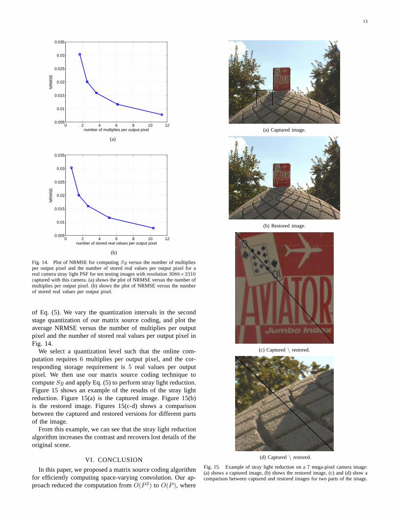
of Eq. (5). We vary the quantization intervals in the secondstage quantization of our matrix source coding, and plot theaverage NRMSE versus the number of multiplies per outputpixel and the number of stored real values per output pixel inFig. 14.

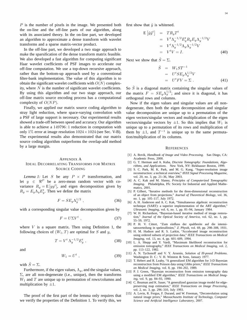
We select a quantization level such that the online com-putation requires6 multiplies per output pixel, and the cor-responding storage requirement is5 real values per outputpixel. We then use our matrix source coding technique tocomputeSy and apply Eq. (5) to perform stray light reduction.Figure 15 shows an example of the results of the stray lightreduction. Figure 15(a) is the captured image. Figure 15(b)is the restored image. Figures 15(c-d) shows a comparisonbetween the captured and restored versions for different partsof the image.

From this example, we can see that the stray light reductionalgorithm increases the contrast and recovers lost detailsof theoriginal scene.

VI. CONCLUSION

In this paper, we proposed a matrix source coding algorithmfor efficiently computing space-varying convolution. Our ap-proach reduced the computation fromO(P 2) to O(P ), where

(a) Captured image.

(b) Restored image.

(c) Captured\ restored.

(d) Captured\ restored.

Fig. 15. Example of stray light reduction on a7 mega-pixel camera image:(a) shows a captured image, (b) shows the restored image, (c)and (d) show acomparison between captured and restored images for two parts of the image.

14

P is the number of pixels in the image. We presented boththe on-line and the off-line parts of our algorithm, alongwith its associated theory. In the on-line part, we developedan algorithm to approximate a dense transform with wavelettransforms and a sparse matrix-vector product.

In the off-line part, we developed a two stage approach tomake the sparsification of the dense transform matrix feasible.We also developed a fast algorithm for computing significantHaar wavelet coefficients of PSF images to accelerate ouroff-line computation. We use a top-down recursive approach,rather than the bottom-up approach used by a conventionalfilter-bank implementation. The value of this algorithm is toobtain the significant wavelet coefficients withO(N) complex-ity, whereN is the number of significant wavelet coefficients.By using this algorithm and our two stage approach, ouroff-line matrix source encoding process has a computationalcomplexity ofO(NP ).

Finally, we applied our matrix source coding algorithm tostray light reduction, where space-varying convolution witha PSF of large support is necessary. Our experimental resultsshowed a trade-off between speed and accuracy. Our algorithmis able to achieve a149796 :1 reduction in computation withonly 1% error at image resolution1024×1024 (see Sec. V-B).The experimental results also demonstrated that our matrixsource coding algorithm outperforms the overlap-add methodby a large margin.

APPENDIX AIDEAL DECORRELATINGTRANSFORMS FORMATRIX

SOURCE CODING

Lemma 1:Let S be any P × P transformation, andlet y ∈ ℜP be a zero-mean random vector with co-variance Ry = E [yyt], and eigen decomposition given byRy = EyΛyE

ty . Then we define the matrix

F = SEyΛ1/2y , (36)

with a corresponding singular value decomposition given by

F = UΣV t , (37)

where V is a square matrix. Then using Definition 1, thefollowing choices of(W1, T ) are optimal forS andy,

T = V t Λ−1/2y Et

y , (38)

and

W1 = U t , (39)

with S = Σ.Furthermore, if the eigen values,Λy, and the singular values,

Σ, are all non-degenerate (i.e., unique), then the transformsW1 andT are unique up to permutation of rows/columns andmultiplication by±1.

The proof of the first part of the lemma only requires thatwe verify the properties of the Definition 1. To verify this, we

first show thaty is whitened.

E[

yyt]

= TRyTt

= V tΛ−1/2y Et

yRyEyΛ−1/2y V

= V tΛ−1/2y ΛyΛ−1/2

y V

= V tV = I. (40)

Next we show thatS = Σ.

S = W1ST−1

= U tSEyΛ1/2y V

= U tFV = Σ . (41)

So S is a diagonal matrix containing the singular values ofthe matrix F = SEyΛ

1/2y ; and since it is diagonal, it has

orthogonal rows and columns.Now if the eigen values and singular values are all non-

degenerate, then both the eigen decomposition and singularvalue decomposition are unique up to a permutation of theeigen vectors/singular vectors and multiplication of the eigenvectors/singular vectors by±1. So this implies thatW1 isunique up to a permutation of its rows and multiplication ofthem by ±1, and T−1 is unique up to the same permuta-tion/multiplication of its columns.

REFERENCES

[1] A. Bovik, Handbook of Image and Video Processing. San Diego, CA:Academic Press, 2000.

[2] G. T. Herman and A. Kuba,Discrete Tomography: Foundations, Algo-rithms, and Applications. New York, NY: Birkhauser Boston, 1999.

[3] S. C. Park, M. K. Park, and M. G. Kang, “Super-resolution imagereconstruction: a technical overview,”IEEE Signal Processing Magazine,vol. 20, no. 3, pp. 21–36, May 2003.

[4] A. C. Kak and M. Slaney,Principles of Computerized TomographicImaging. Philadelphia, PA: Society for Industrial and Applied Mathe-matics, 2001.

[5] P. Gilbert, “Iterative methods for the three-dimensional reconstructionof an object from projections,”Journal of Theoretical Biology, vol. 36,no. 1, pp. 105–117, July 1972.

[6] A. H. Anderson and A. C. Kak, “Simultaneous algebraic reconstructiontechnique (SART): a superior implementation of the ART algorithm,”Ultrasonic Imaging, vol. 6, no. 1, pp. 81–94, January 1984.

[7] W. H. Richardson, “Bayesian-based iterative method of image restora-tion,” Journal of the Optical Society of America, vol. 62, no. 1, pp.55–59, 1972.

[8] P. H. V. Cittert, “Zum einfluss der spaltbreite auf die intensi-tatswerteilung in spektrallinien,”Z. Physik, vol. 69, pp. 298–308, 1931.

[9] H. M. Hudson and R. S. Larkin, “Accelerated image reconstructionusing ordered subsets of projection data,”IEEE Transactions on MedicalImaging, vol. 13, no. 4, pp. 601–609, 1994.

[10] L. A. Shepp and Y. Vardi, “Maximum likelihood reconstruction foremission tomography,”IEEE Transactions on Medical Imaging, vol. 2,pp. 113–122, 1982.

[11] A. N. Tychonoff and V. Y. Arsenin,Solution of Ill-posed Problems.Washington D. C.: V. H. Winston & Sons, January 1977.

[12] T. Hebert and R. Leahy, “A generalized EM algorithm for 3-D Bayesianreconstruction from Poisson data using Gibbs priors,”IEEE Transactionson Medical Imaging, vol. 8, pp. 194–202, 1989.

[13] P. J. Green, “Bayesian reconstruction from emission tomography datausing a modified EM algorithm,”IEEE Transactions on Medical Imag-ing, vol. 9, pp. 84–93, 1990.

[14] C. Bouman and K. Sauer, “A generalized gaussian image model for edge-preserving map estimation,”IEEE Transactions on Image Processing,vol. 2, no. 3, pp. 296–310, July 1993.

[15] A. Levin, R. Fergus, F. Durand, and W. Freeman, “Deconvolution usingnatural image priors,”Massachusetts Institute of Technology, ComputerScience and Artificial Intelligence Laboratory, 2007.

15

[16] D. Krishnan and R. Fergus, “Fast image deconvolution using hyper-Laplacian priors,”Advances in Neural Information Processing Systems,pp. 1033–1041, 2009.

[17] D. Zoran and Y. Weiss, “From learning models of natural image patchesto whole image restoration,” in2011 IEEE International Conference onComputer Vision, 2011, pp. 479–486.

[18] U. Schmidt, K. Schelten, and S. Roth, “Bayesian deblurring withintegrated noise estimation,” in2011 IEEE Conference on ComputerVision and Pattern Recognition, 2011, pp. 2625–2632.

[19] C. Schuler, H. Burger, S. Harmeling, and B. Scholkopf, “A machinelearning approach for non-blind image deconvolution,” in2013 IEEEConference on Computer Vision and Pattern Recognition, 2013.

[20] C. Lanczos,Linear Differential Operators. Mineola, NY: DoverPublications, 1997.

[21] S. Mallat, A Wavelet Tour of Signal Processing. San Diego, CA:Academic Press, 1998.

[22] J. W. Cooley and J. W. Tukey, “An algorithm for the machine calculationof complex Fourier series,”Mathematics of Computation, vol. 19, no. 90,April 1965.

[23] J. Wei, B. Bitlis, A. Bernstein, A. Silva, P. A. Jansson,and J. P. Allebach,“Stray light and shading reduction in digital photography –a new modeland algorithm,” inProceedings of the SPIE/IS&T Conference on DigitalPhotography IV, vol. 6817, San Jose, CA, January 2008.

[24] W. J. Smith, Modern Optical Engineering : the Design of OpticalSystems. New York, NY: McGraw Hill, 2000.

[25] P. A. Jansson and J. H. Fralinger, “Parallel processingnetwork thatcorrects for light scattering in image scanners,”U.S. Patent 5,153,926,1992.

[26] T. G. Stockham, “High-speed convolution and correlation,” in Proceed-ings of the April 26-28, 1966, Spring joint computer conference, 1966,pp. 229–233.

[27] J. G. Nagy and D. P. O’Leary, “Fast iterative image restoration with aspatially varying PSF,” inProceedings of SPIE Conference on AdvancedSignal Processin g: Algorithms, Architectures, and Implementations VII,vol. 3162, San Diego, CA, 1997, pp. 388–399.

[28] J. Bardsley, S. Jefferies, J. Nagy, and R. Plemmons, “A computationalmethod for the restoration of images with an unknown, spatially-varyingblur,” Optics Express, vol. 15, no. 5, pp. 1767–1782, 2006.

[29] M. Hirsch, S. Sra, B. Scholkopf, and S. Harmeling, “Efficient filter flowfor space-variant multiframe blind deconvolution,” inProceedings of2010 IEEE Conference on Computer Vision and Pattern Recognition,2010, pp. 607–614.

[30] E. Gilad and J. von Hardenberg, “A fast algorithm for convolutionintegrals with space and time variant kernels,”Journal of ComputationalPhysics, vol. 216, pp. 326–336, 2006.

[31] L. Denis, E. Thiebaut, and F. Soulez, “Fast model of space-variantblurring and its application to deconvolution in astronomy,” in 201118th IEEE International Conference on Image Processing, 2011, pp.2817–2820.

[32] J. Wei, G. Cao, C. A. Bouman, and J. P. Allebach, “Fast space-varyingconvolution and its application in stray light reduction,”in Proceedingsof the SPIE/IS&T Conference on Computational Imaging VII, vol. 7246,San Jose, CA, February 2009.

[33] G. H. Golub and C. F. V. Loan,Matrix Computations. Baltimore,Maryland: The Johns Hopkins University Press, 1996.

[34] G. Cao, C. A. Bouman, and K. J. Webb, “Fast and efficient stored matrixtechniques for optical tomography,” inProceedings of the 40th AsilomarConference on Signals, Systems, and Computers, October 2006.

[35] ——, “Results in non-iterative map reconstruction for optical tomogra-phy,” in Proceedings of the SPIE/IS&T Conference on ComputationalImaging VI, vol. 6814, San Jose, CA, January 2008.

[36] D. Tretter and C. A. Bouman, “Optimal transforms for multispectraland multilayer image coding,”IEEE Transactions on Image Processing,vol. 4, no. 3, pp. 296–308, 1995.

[37] D. Taubman and M. Marcellin,JPEG2000: Image Compression Fun-damentals, Standards and Practice. Norwell, MA: Kluwer AcademicPublishers, 2002.

[38] B. Bitlis, P. A. Jansson, and J. P. Allebach, “Parametric point spreadfunction modeling and reduction of stray light effects in digital stillcameras,” inProceedings of the SPIE/IS&T Conference on Computa-tional Imaging VI, vol. 6498, San Jose, CA, January 2007.

[39] P. A. Jansson, “Method, program, and apparatus for efficiently removingstray-flux effects by selected-ordinate image processing,” U.S. Patent6,829,393, 2004.

[40] P. A. Jansson and R. P. Breault, “Correcting color-measurement errorcaused by stray light in image scanners,” inProceedings of the Sixth

Color Imaging Conference: Color Science, Systems, and Applications,Scottsdale, AZ, November 1998.

[41] P. A. Jansson,Deconvolution of Images and Spectra. New York, NY:Academic Press, 1996.

[42] P. S. R. Diniz, E. A. B. da Silva, and S. L. Netto,Digital SignalProcessing System Analysis and Design. New York, NY: CambridgeUniversity Press, 2002.

Jianing Wei received a B.S. degree from ShanghaiJiao Tong University in 2005, and a Ph.D. degreein Electrical Engineering from Purdue University in2010. His Ph.D. work includes stray light reductionin digital cameras, algorithms for fast space-varyingconvolution, and functional MRI analysis. Between2009 and 2013, he was with the U.S. ResearchCenter of Sony Corporation, San Jose, CA, wherehe focused on computer vision and image process-ing algorithm development for digital cameras andtelevisions. Dr. Wei joined Google Inc., Mountain

View, CA, in 2013, where he is currently a software engineer working onimaging algorithm development for android cameras.

Charles A. Bouman received a B.S.E.E. degreefrom the University of Pennsylvania in 1981 anda MS degree from the University of California atBerkeley in 1982. From 1982 to 1985, he was afull staff member at MIT Lincoln Laboratory and in1989 he received a Ph.D. in electrical engineeringfrom Princeton University. He joined the faculty ofPurdue University in 1989 where he is currentlythe Michael J. and Katherine R. Birck Professor ofElectrical and Computer Engineering. He also holdsa courtesy appointment in the School of Biomedical

Engineering and is co-director of Purdue’s Magnetic Resonance ImagingFacility located in Purdue’s Research Park.

Professor Bouman’s research focuses on the use of statistical imagemodels, multiscale techniques, and fast algorithms in applications includingtomographic reconstruction, medical imaging, and document rendering andacquisition. Professor Bouman is a Fellow of the IEEE, a Fellow of theAmerican Institute for Medical and Biological Engineering(AIMBE), aFellow of the society for Imaging Science and Technology (IS&T), a Fellowof the SPIE professional society. He is also a recipient of IS&T’s RaymondC. Bowman Award for outstanding contributions to digital imaging educationand research, has been a Purdue University Faculty Scholar,received theCollege of Engineering Engagement/Service Award, and TeamAward, andin 2014 he received the Electronic Imaging Scientist of the Year award.He was previously the Editor-in-Chief for the IEEE Transactions on ImageProcessing and a Distinguished Lecturer for the IEEE SignalProcessingSociety, and he is currently the Vice President of TechnicalActivities forIEEE Signal Processing Society. He has been an associate editor for theIEEE Transactions on Image Processing and the IEEE Transactions on PatternAnalysis and Machine Intelligence. He has also been Co-Chair of the 2006SPIE/IS&T Symposium on Electronic Imaging, Co-Chair of theSPIE/IS&Tconferences on Visual Communications and Image Processing2000 (VCIP),a Vice President of Publications and a member of the Board of Directorsfor the IS&T Society, and he is the founder and Co-Chair of theSPIE/IS&Tconference on Computational Imaging.

16

Jan P. Allebach is Hewlett-Packard DistinguishedProfessor of Electrical and Computer Engineering atPurdue University. His current research interests in-clude image rendering, image quality, color imagingand color measurement, document aesthetics, andprinter forensics. Allebach is a Fellow of the IEEE,the Society for Imaging Science and Technology(IS&T), and SPIE. He was named Electronic Imag-ing Scientist of the Year by IS&T and SPIE, andwas named Honorary Member of IS&T, the highestaward that IS&T bestows. He was the recipient of

the 2013 IEEE Daniel E. Noble Award, and was elected to membership inthe National Academy of Engineers in 2014, both on the basis of his workon digital halftoning.