Fast Spatially-Varying Indoor Lighting Estimation

Mathieu Garon⋆*, Kalyan Sunkavalli†, Sunil Hadap†, Nathan Carr†, Jean-Francois Lalonde⋆

⋆Universite Laval, †Adobe Research

mathieu.garon.2@ulaval.ca {sunkaval, hadap, ncarr}@adobe.com jflalonde@gel.ulaval.ca

Abstract

We propose a real-time method to estimate spatially-

varying indoor lighting from a single RGB image. Given an

image and a 2D location in that image, our CNN estimates a

5th order spherical harmonic representation of the lighting

at the given location in less than 20ms on a laptop mobile

graphics card. While existing approaches estimate a single,

global lighting representation or require depth as input, our

method reasons about local lighting without requiring any

geometry information. We demonstrate, through quantitative

experiments including a user study, that our results achieve

lower lighting estimation errors and are preferred by users

over the state-of-the-art. Our approach can be used directly

for augmented reality applications, where a virtual object is

relit realistically at any position in the scene in real-time.

1. Introduction

Estimating the illumination conditions of a scene is a

challenging problem. An image is formed by conflating

the effects of lighting with those of scene geometry, surface

reflectance, and camera properties. Inverting this image

formation process to recover lighting (or any of these other

intrinsic properties) is severely underconstrained. Typical

solutions to this problem rely on inserting an object (a light

probe) with known geometry and/or reflectance properties

in the scene (a shiny sphere [5], or 3D objects of known

geometry [9, 34]). Unfortunately, having to insert a known

object in the scene is limiting and thus not easily amenable

to practical applications.

Previous work has tackled this problem by using addi-

tional information such as depth [1, 25], multiple images

acquired by scanning a scene [12, 26, 36, 37] or user in-

put [18]. However, such information is cumbersome to ac-

quire. Recent work [8] has proposed a learning approach

that bypasses the need for additional information by predict-

ing lighting directly from a single image in an end-to-end

*Parts of this work were completed while Mathieu Garon was an intern

at Adobe Research.

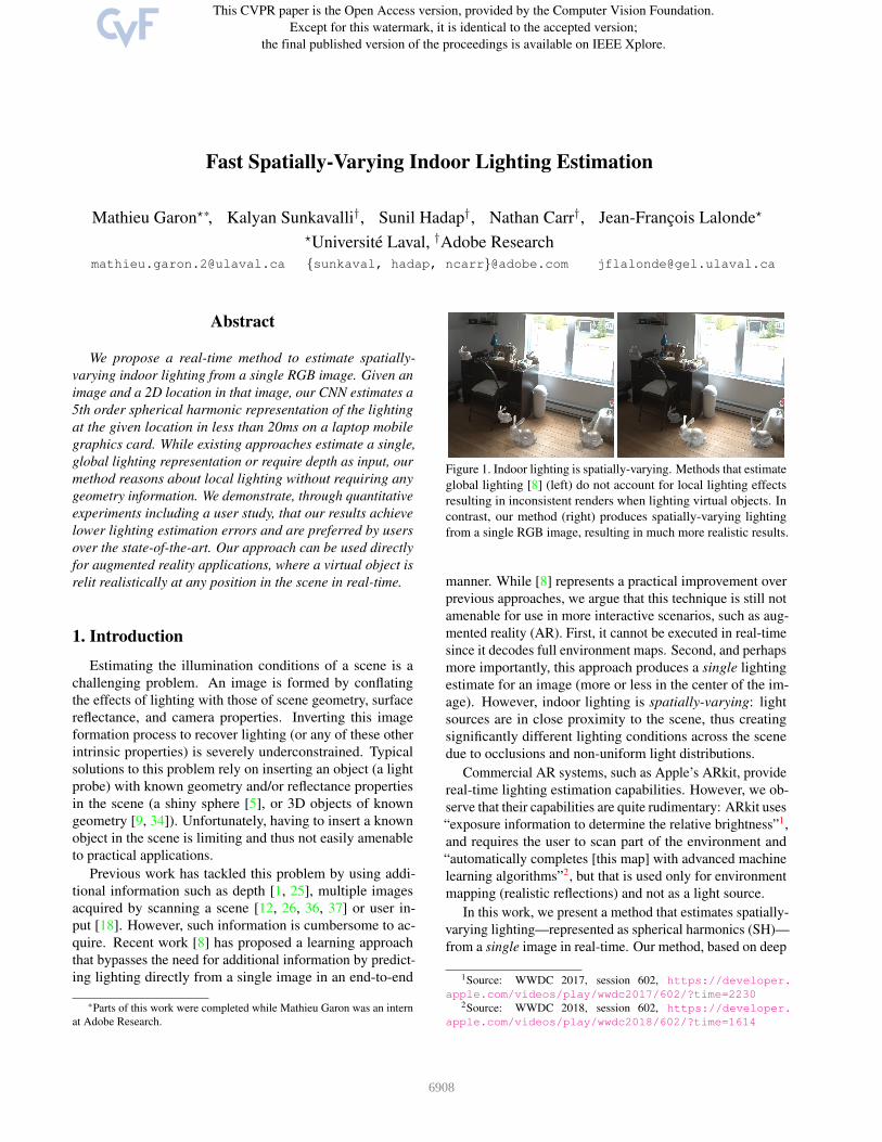
Figure 1. Indoor lighting is spatially-varying. Methods that estimate

global lighting [8] (left) do not account for local lighting effects

resulting in inconsistent renders when lighting virtual objects. In

contrast, our method (right) produces spatially-varying lighting

from a single RGB image, resulting in much more realistic results.

manner. While [8] represents a practical improvement over

previous approaches, we argue that this technique is still not

amenable for use in more interactive scenarios, such as aug-

mented reality (AR). First, it cannot be executed in real-time

since it decodes full environment maps. Second, and perhaps

more importantly, this approach produces a single lighting

estimate for an image (more or less in the center of the im-

age). However, indoor lighting is spatially-varying: light

sources are in close proximity to the scene, thus creating

significantly different lighting conditions across the scene

due to occlusions and non-uniform light distributions.

Commercial AR systems, such as Apple’s ARkit, provide

real-time lighting estimation capabilities. However, we ob-

serve that their capabilities are quite rudimentary: ARkit uses

“exposure information to determine the relative brightness”1,

and requires the user to scan part of the environment and

“automatically completes [this map] with advanced machine

learning algorithms”2, but that is used only for environment

mapping (realistic reflections) and not as a light source.

In this work, we present a method that estimates spatially-

varying lighting—represented as spherical harmonics (SH)—

from a single image in real-time. Our method, based on deep

1Source: WWDC 2017, session 602, https://developer.

apple.com/videos/play/wwdc2017/602/?time=22302Source: WWDC 2018, session 602, https://developer.

apple.com/videos/play/wwdc2018/602/?time=1614

6908

learning, takes as input a single image and a 2D location in

that image, and outputs the 5th-order SH coefficients for the

lighting at that location. Our approach has three main ad-

vantages. First, spherical harmonics are a low-dimensional

lighting representation (36 values for 5th-degree SH for each

color channel), and can be predicted with a compact decoder

architecture. Indeed, our experiments demonstrate that our

network can predict 5th-degree SH coefficients in less than

20ms on a mobile GPU (Nvidia GTX970M). Second, the

SH coefficients can directly be used by off-the-shelf shaders

to achieve real-time relighting [28, 32]. Third, and perhaps

more importantly, these local SH estimates directly embed

local light visibility without the need for explicit geometry

estimates. Our method therefore adapts to local occlusions

and reflections without having to conduct an explicit reason-

ing on scene geometry. Note that while using SH constrains

the angular frequency of the lighting we can represent, by

having a different estimate for every scene location, our

method does capture high-frequency spatial variations such

as the shadowing under the desk in Figure 1(b).

To the best of our knowledge, our paper is the first to

propose a practical approach for estimating spatially-varying

lighting from a single indoor RGB image. Our approach en-

ables a complete image-to-render augmented reality pipeline

that automatically adapts to both local and global light-

ing changes at real-time framerates. In order to evaluate

spatially-varying methods quantitatively, a novel, challeng-

ing dataset containing 79 ground truth HDR light probes in

a variety of indoor scenes is made publicly available3.

2. Related work

Estimating lighting from images has a long history in

computer vision and graphics. In his pioneering work, De-

bevec proposed to explicitly capture HDR lighting from a

reflective metallic sphere inserted into the scene [5].

A large body of work relies on more generic 3D objects

present in the scene to estimate illumination. Notably, Bar-

ron and Malik [2] model object appearance as a combination

of its shape, lighting, and material properties, and attempt to

jointly estimate all of these properties in an inverse rendering

framework which relies on data-driven priors to compensate

for the lack of information available in a single image. Sim-

ilarly, Lombardi and Nishino [24] estimate reflectance and

illumination from an object of known shape. Prior work has

also used faces in images to estimate lighting [3].

More recently, Georgoulis et al. [10] use deep learning to

estimate lighting and reflectance from an object of known

geometry, by first estimating its reflectance map (i.e., its

“orientation-dependent” appearance) [30] and factoring it

into lighting and material properties [9] afterwards.

Within the context of AR, real-time approaches [12, 26]

3https://lvsn.github.io/fastindoorlight/

model the Radiance Transfer Function of an entire scene

from its captured geometry, but require that the scene be

reconstructed first. Zhang et al. [36] also recover spatially-

varying illumination, but require a complete scene recon-

struction and user-annotated light positions. In more recent

work, the same authors [37] present a scene transform that

identifies likely isotropic point light positions from the shad-

ing they create on flat surfaces, acquired using similar scene

scans. Other methods decompose an RGBD image into its in-

trinsic scene components [1, 25] including spatially-varying

SH-based lighting. In contrast, our work does not require any

knowledge of scene geometry, and automatically estimates

spatially-varying SH lighting from a single image.

Methods which estimate lighting from single images have

also been proposed. Khan et al. [20] propose to flip an HDR

input image to approximate the out-of-view illumination.

Similar ideas have been used for compositing [22]. While

these approximations might work in the case of mostly dif-

fuse lighting, directional lighting cannot be estimated reli-

ably, for example, if the dominant light is outside the field of

view of the camera. Karsch et al. [18] develop a user-guided

system, yielding high quality lighting estimates. In subse-

quent work [19], the same authors propose an automatic

method that matches the background image with a large

database of LDR panoramas, and optimizes light positions

and intensities in an inverse rendering framework that relies

on an intrinsic decomposition of the scene and automatic

depth estimation. Lalonde et al. [21] estimate lighting by

combining cues such as shadows and shading from an image

in a probabilistic framework, but their approach is targeted

towards outdoor scenes. Hold-Geoffroy et al. [14] recently

provided a more robust method of doing so by relying on

deep neural networks trained to estimate the parameters of

an outdoor illumination model.

More closely related to our work, Gardner et al. [8] esti-

mate indoor illumination from a single image using a neural

network. Their approach is first trained on images extracted

from a large set of LDR panoramas in which light sources

are detected. Then, they fine-tune their network on HDR

panoramas. Similarly, Cheng et al. [4] proposed estimating

SH coefficients given two images captured from the front

and back camera of a mobile device. However, both of these

works provide a single, global lighting estimate for an entire

image. In contrast, we predict spatially-varying lighting.

3. Dataset

In order to learn to estimate local lighting, we need a

large database of images and their corresponding illumina-

tion conditions (light probes) measured at several locations

in the scene. Relying on panorama datasets such as [8]

unfortunately cannot be done since they do not capture lo-

cal occlusions. While we provide a small dataset of real

photographs for the evaluation of our approach (sec. 5.2),

6909

1

3

2

1 32 Lighting

Depth

1

3

2

1 32 Lighting

Depth

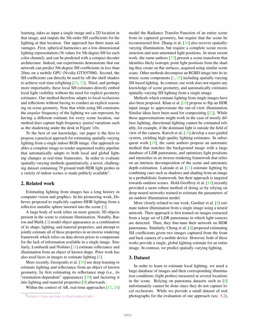
Figure 2. Example synthetic light probes sampled in our dataset.

Locations on the image are randomly sampled (left). For each

location, light probes (right, top) and their corresponding depth

maps (right, bottom) are rendered into cube maps.

capturing enough such images to train a neural network

would require a large amount of ressources. We therefore

rely on realistic, synthetic data to train our neural network.

In this section, we describe how we create our local light

probe training data.

3.1. Rendering images

As in [38], we use the SUNCG [33] dataset for training.

We do not use the Reinhard tonemapping algorithm [29]

and instead use a simple gamma [23]. We now describe the

corrections applied to the renders to improve their realism.

The intensity of the light sources in the SUNCG dataset

are randomly scaled by a factor e ∼ U [100, 500], where

U [a, b] is a uniform distribution in the [a, b] interval.

Since many scenes have windows, we randomly sample

a panorama from a dataset of 200 HDR outdoor panora-

mas [13]. Each outdoor panorama is also randomly rotated

about its vertical axis, to simulate different sun directions.

We found the use of these panoramas to add significant real-

ism to scenes with a window, providing realistic appearance

and lighting distributions (see fig. 2).

We render a total of 26,800 images, and use the same

scenes and camera viewpoints as [38]. Care is taken to split

the training/validation dataset according to houses (each

house containing many rooms). Each image is rendered at

640×480 resolution using the Metropolis Light Transport

(MLT) algorithm of Mitsuba [17], with 512 samples.

3.2. Rendering local light probes

For each image, we randomly sample 4 locations in the

scene to render the local light probes. The image is split

into 4 quadrants, and a random 2D coordinate is sampled

uniformly in each quadrant (excluding a 5% border around

the edges of the image). To determine the position of the

virtual camera in order to render the light probe (the “probe

camera”), a ray is cast from the scene camera to the image

plane, and the first intersection point with geometry is kept.

From that point, we move the virtual camera 10cm away

from the surface, along the normal, and render the light

probe at this location. Note that the probe camera axes are

aligned with those of the scene camera—only a translation

is applied.

Each light probe is rendered in the cubemap represen-

tation, rendering each of the 6 faces independently. While

Mitsuba MLT can converge to a realistic image rapidly, it

sometimes converges to a wrong solution that can nega-

tively affect the ground truth probes. Thus, for each face

we use the Bidirectional Path Tracing (BDPT) algorithm

of Mitsuba [17], with 1,024 samples and render at 64×64resolution. This takes, on average, 5 minutes to render all 6

faces of a light probe. In addition, we also render the depth

at each probe. Fig. 2 shows examples of images and their

corresponding probes in our synthetic dataset.

After rendering, scenes are filtered out to remove erro-

neous floor or wall area lights which are present in SUNCG.

In addition, moving 10cm away from a surface may result

in the camera being behind another surface. To filter these

probes out, we simply threshold based on the mean light

probe intensity (a value of 0.01 was found empirically). Fi-

nally, we fit 5th order SH coefficients to the rendered light

and depth probes to obtain ground truth values to learn.

4. Learning to estimate local indoor lighting

4.1. Main architecture for lighting estimation

We now describe our deep network architecture to learn

spatially-varying lighting from an image. Previous work has

shown that global context can help in conducting reasoning

on lighting [8], so it is likely that a combination of global

and local information will be needed here.

Our proposed architecture is illustrated in fig. 3. We

require an input RGB image of 341× 256 resolution and a

specific coordinate in the image where the lighting is to be

estimated. The image is provided to a “global” path in the

CNN. A local patch of 150 × 150 resolution, centered on

that location, is extracted and fed to a “local” path.

The global path processes the input image via the three

first blocks of a pretrained DenseNet-121 network to gen-

erate a feature map. A binary coordinate mask, of spatial

resolution 16× 21, with the elements corresponding to the

local patch set to 1 and 0 elsewhere, is concatenated as an

additional channel to the feature map. The result is fed to

an encoder, which produces a 5120-dimensional vector zg.

The local path has a similar structure. It processes the input

patch with a pretrained DenseNet-121 network to generate

a feature map, which is fed to an encoder and produces a

512-dimensional vector zl. Both global and local encoders

share similar structures and use Fire modules [16]. With

the fire-x-y notation, meaning that the module reduces the

6910

Global

Encoder

DenseNet 121(3 blocks)

Encoder

DenseNet 121(3 blocks)

Local FC FC

zl

zg

zi

Coordinate mask

1025x16x21

1024x9x9

5120

5121024

Real orSynthetic?

Lighting SH

Albedo

Shading

36

4x4x4

36x3

Depth SH

3x150x150

3x341x256

GRL

Decoder

Discriminator

FC FC FC

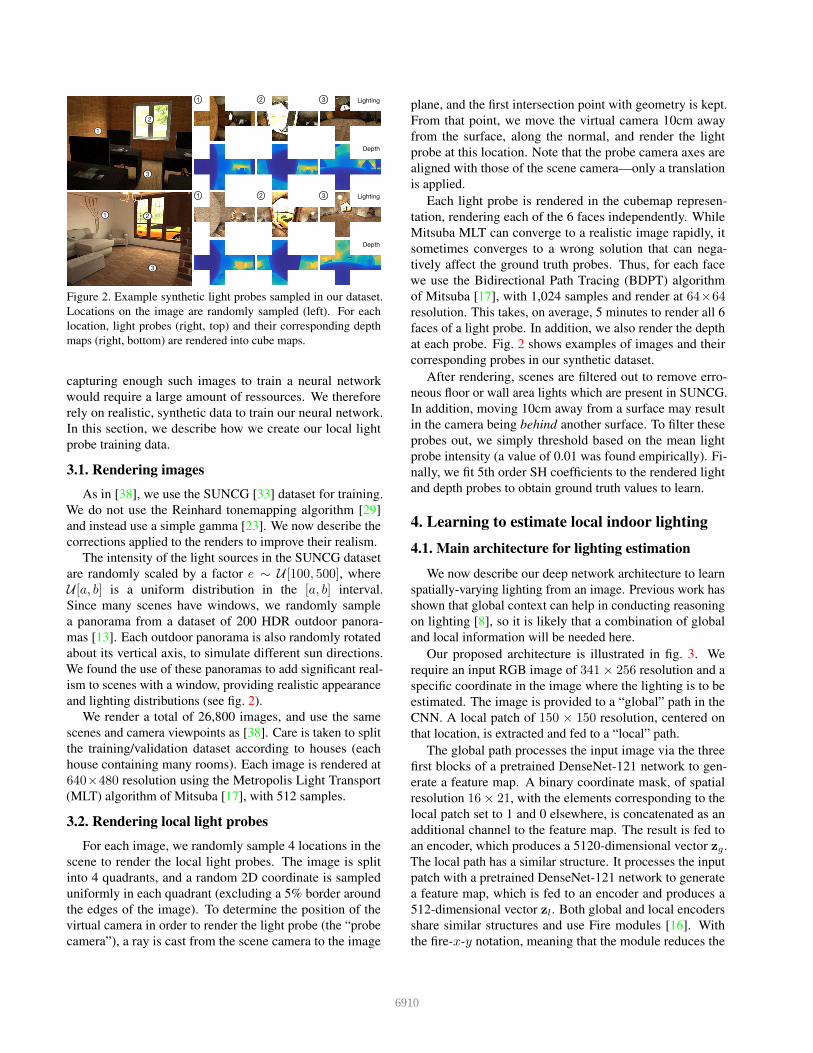
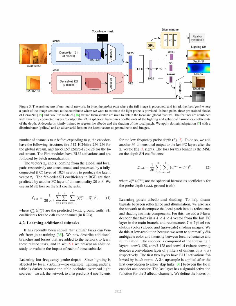
Figure 3. The architecture of our neural network. In blue, the global path where the full image is processed, and in red, the local path where

a patch of the image centered at the coordinate where we want to estimate the light probe is provided. In both paths, three pre-trained blocks

of DenseNet [15] and two Fire modules [16] trained from scratch are used to obtain the local and global features. The features are combined

with two fully connected layers to output the RGB spherical harmonics coefficients of the lighting and spherical harmonics coefficients

of the depth. A decoder is jointly trained to regress the albedo and the shading of the local patch. We apply domain adaptation [7] with a

discriminator (yellow) and an adversarial loss on the latent vector to generalize to real images.

number of channels to x before expanding to y, the encoders

have the following structure: fire-512-1024/fire-256-256 for

the global stream, and fire-512-512/fire-128-128 for the lo-

cal stream. The Fire modules have ELU activations and are

followed by batch normalization.

The vectors zg and zl coming from the global and local

paths respectively are concatenated and processed by a fully-

connected (FC) layer of 1024 neurons to produce the latent

vector zi. The 5th-order SH coefficients in RGB are then

predicted by another FC layer of dimensionality 36× 3. We

use an MSE loss on the SH coefficients:

Li-sh =1

36× 3

3∑

c=1

4∑

l=0

l∑

m=−l

(im∗

l,c − iml,c)2 , (1)

where iml,c (im∗

l,c ) are the predicted (w.r.t. ground truth) SH

coefficients for the c-th color channel (in RGB).

4.2. Learning additional subtasks

It has recently been shown that similar tasks can ben-

efit from joint training [35]. We now describe additional

branches and losses that are added to the network to learn

these related tasks, and in sec. 5.1 we present an ablation

study to evaluate the impact of each of these subtasks.

Learning low-frequency probe depth Since lighting is

affected by local visibility—for example, lighting under a

table is darker because the table occludes overhead light

sources—we ask the network to also predict SH coefficients

for the low-frequency probe depth (fig. 2). To do so, we add

another 36-dimensional output to the last FC layers after the

zi vector (fig. 3, right). The loss for this branch is the MSE

on the depth SH coefficients:

Ld-sh =1

36

4∑

l=0

l∑

m=−l

(dm∗

l − dml )2 , (2)

where dml (dm∗

l ) are the spherical harmonics coefficients for

the probe depth (w.r.t. ground truth).

Learning patch albedo and shading To help disam-

biguate between reflectance and illumination, we also ask

the network to decompose the local patch into its reflectance

and shading intrinsic components. For this, we add a 3-layer

decoder that takes in a 4 × 4 × 4 vector from the last FC

layer in the main branch, and reconstructs 7 × 7 pixel res-

olution (color) albedo and (grayscale) shading images. We

do this at low-resolution because we want to summarily dis-

ambiguate color and intensity between local reflectance and

illumination. The encoder is composed of the following 3

layers: conv3-128, conv3-128 and conv1-4 (where convx-ydenotes a convolution layer of y filters of dimension x× x)

respectively. The first two layers have ELU activations fol-

lowed by batch norm. A 2× upsample is applied after the

first convolution to allow skip links [31] between the local

encoder and decoder. The last layer has a sigmoid activation

function for the 3 albedo channels. We define the losses on

6911

reflectance and shading as:

Lrs-mse =1

N

N∑

i=1

(R∗

i −Ri)2 + (S∗

i − Si)2

Lrs-recons =1

N

N∑

i=1

(P∗

i − (Ri + Si))2

, (3)

where Ri (R∗

i ) and Si (S∗

i ) denote the log-reflectance pre-

diction (resp. ground truth) and log-shading prediction (resp.

ground truth) respectively, and P∗

i is the input patch.

Adapting to real data We apply unsupervised domain

adaptation [7] to adapt the model trained on synthetic

SUNCG images to real photographs. This is done via a

discriminator connected to the zi latent vector by a gradient

reversal layer (GRL). The discriminator, illustrated in the

top-right of fig. 3, is composed of 3 FC layers of (64, 32, 2)

neurons respectively, with the ELU activation and the first

two layers followed by batch normalization. We train the

discriminator with the cross-entropy loss:

Lda = −

N∑

i=1

r∗i log ri , (4)

where ri (r∗i ) is the discriminator output (resp. ground truth).

4.3. Training

The overall loss for our neural network is a linear combi-

nation of the individual losses introduced in sec. 4.2:

L = Li-sh + Ld-sh + Lrs-mse + Lrs-recons + λLda . (5)

Here, λ = 2/(1+ exp(−8n/60))− 1, where n is the epoch,

is a weight controlling the importance of the domain adapta-

tion loss, which becomes asymptotically closer to 1 as the

number of training epochs e increases. We train the network

from scratch (apart for the DenseNet-121 blocks which are

pretrained on ImageNet) using the Adam optimizer with

β = (0.9, 0.999). We employ a learning rate of 10−4 for the

first 60 epochs, and of 10−5 for 30 additional epochs.

The network is trained on a combination of synthetic and

real data. Each minibatch, of total size 20, is composed of

50% synthetic, and 50% real data. For the synthetic data,

all losses in eq. (5) are activated. In total, we use 83,812

probes from 24,000 synthetic images for training, and 9,967

probes from 2,800 images for validation (to monitor for over-

fitting). We augment the synthetic data (images and probes)

at runtime, while training the network, using the following

three strategies: 1) horizontal flip; 2) random exposure factor

f ∼ U [0.16, 3], where U [a, b] is the uniform distribution in

the [a, b] interval as in sec. 3; and 3) random camera response

function f(x) = x1/γ , γ ∼ U [1.8, 2.4]. The real data is

composed of crops extracted from the Laval Indoor HDR

dataset [8]. Since we do not have any ground truth for the

real data, we only employ the Lda loss in this case.

SH DegreeGlobal

(w/o mask)

Global

(w mask)Local

Local + Global

(w mask)

0 0.698 0.563 0.553 0.520

1 0.451 0.384 0.412 0.379

2–5 0.182 0.158 0.165 0.159

Table 1. Ablation study on the network inputs. The mean absolute

error (MAE) of each SH degree on the synthetic test set are reported.

“Global w/o mask” takes the full image without any probe position

information. Two types of local information are evaluated: “Global

(w mask)” receives the full image and the coordinate mask of the

probe position, and “Local” receives a patch around the probe

position. Our experiments show that using both local information

and the full image (“Local + Global (w mask”) reduces the error.

SH Degree Li-sh +Ld-sh+Lrs-mse

+Lrs-reconsAll

0 0.520 0.511 0.472 0.449

1 0.379 0.341 0.372 0.336

2–5 0.159 0.149 0.166 0.146

Degree 1 angle 0.604 0.582 0.641 0.541

Table 2. Comparing the mean absolute error (MAE) of the lighting

SH degrees for each loss from 10,000 synthetic test probes. Es-

timating the low frequency depth at the probe position improves

the directional degrees of the SH while providing minimal gain

on the ambient light (degree 0). The albedo and shading losses

improve the ambient light estimation. “Degree 1 angle” represents

the angular error of the first order SH. Training the network on all

of these tasks achieves better results for all of the degrees.

5. Experimental validation

We now present an extensive evaluation of our network

design as well as qualitative and quantitative results on a

new benchmark test set. We evaluate our system’s accuracy

at estimating 5th order SH coefficients. We chose order 5

after experimenting with orders ranging from 3 to 8, and

empirically confirming that order 5 SH lighting gave us a

practical trade-off between rendering time and visual qual-

ity (including shading and shadow softness). In principle,

our network can be easily extended to infer higher order

coefficients.

5.1. Validation on synthetic data

A non-overlapping test set of 9,900 probes from 2,800

synthetic images (sec. 3) is used to perform two ablation

studies to validate the design choices in the network archi-

tecture (sec. 4.1) and additional subtasks (sec. 4.2).

First, we evaluate the impact of having both global and

local paths in the network, and report the mean absolute

error (MAE) in SH coefficient estimation in tab. 1. For this

experiment, the baseline (“Global (w/o mask)”) is a network

that receives only the full image, similar to Gardner et al. [8].

Without local information, the network predicts the average

light condition of the scene and fails to predict local changes,

thus resulting in low accuracy. Lower error is obtained by

concatenating the coordinate mask to the global DenseNet

6912

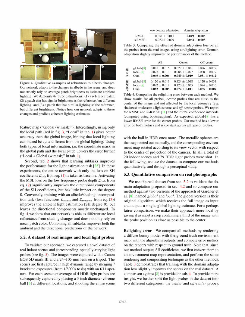
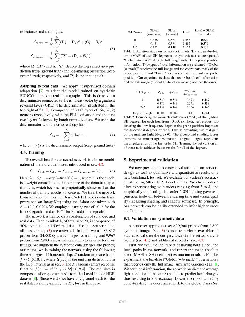
Figure 4. Qualitative examples of robustness to albedo changes.

Our network adapts to the changes in albedo in the scene, and does

not strictly rely on average patch brightness to estimate ambient

lighting. We demonstrate three estimations: (1) a reference patch,

(2) a patch that has similar brightness as the reference, but different

lighting; and (3) a patch that has similar lighting as the reference,

but different brightness. Notice how our network adapts to these

changes and predicts coherent lighting estimates.

feature map (“Global (w mask)”). Interestingly, using only

the local path (red in fig. 3, “Local” in tab. 1) gives better

accuracy than the global image, hinting that local lighting

can indeed be quite different from the global lighting. Using

both types of local information, i.e. the coordinate mask in

the global path and the local patch, lowers the error further

(“Local + Global (w mask)” in tab. 1).

Second, tab. 2 shows that learning subtasks improves

the performance for the light estimation task [35]. In these

experiments, the entire network with only the loss on SH

coefficients Li-sh from eq. (1) is taken as baseline. Activating

the MSE loss on the low frequency probe depth Ld-sh from

eq. (2) significantly improves the directional components

of the SH coefficients, but has little impact on the degree

0. Conversely, training with an albedo/shading decomposi-

tion task (loss functions Lrs-mse and Lrs-recons from eq. (3))

improves the ambient light estimation (SH degree 0), but

leaves the directional components mostly unchanged. In

fig. 4,we show that our network is able to differentiate local

reflectance from shading changes and does not only rely on

mean patch color. Combining all subtasks improves both the

ambient and the directional predictions of the network.

5.2. A dataset of real images and local light probes

To validate our approach, we captured a novel dataset of

real indoor scenes and corresponding, spatially-varying light

probes (see fig. 5). The images were captured with a Canon

EOS 5D mark III and a 24–105 mm lens on a tripod. The

scenes are first captured in high dynamic range by merging 7

bracketed exposures (from 1/8000s to 8s) with an f/11 aper-

ture. For each scene, an average of 4 HDR light probes are

subsequently captured by placing a 3-inch diameter chrome

ball [6] at different locations, and shooting the entire scene

w/o domain adaptation domain adaptation

RMSE 0.051 ± 0.011 0.049 ± 0.006

siRMSE 0.072 ± 0.009 0.062 ± 0.005

Table 3. Comparing the effect of domain adaptation loss on all

the probes from the real images using a relighting error. Domain

adaptation slightly improves the performances of the method.

All Center Off-center

RM

SE global-[8] 0.081 ± 0.015 0.079 ± 0.021 0.086 ± 0.019

local-[8] 0.072 ± 0.013 0.086 ± 0.027 0.068 ± 0.019

Ours 0.049 ± 0.006 0.049 ± 0.019 0.051 ± 0.012

siR

MS

E global-[8] 0.120 ± 0.013 0.124 ± 0.018 0.120 ± 0.031

local-[8] 0.092 ± 0.017 0.120 ± 0.035 0.084 ± 0.016

Ours 0.062 ± 0.005 0.072 ± 0.011 0.055 ± 0.009

Table 4. Comparing the relighting error between each method. We

show results for all probes, center probes that are close to the

center of the image and not affected by the local geometry (e.g.

shadows) or close to a light source, and off-center probes. We report

the RMSE and si-RMSE [11] and their 95% confidence intervals

(computed using bootstrapping). As expected, global-[8] has a

lower RMSE error for the center probes. Our method has a lower

error on both metrics and is constant across all type of probes.

with the ball in HDR once more. The metallic spheres are

then segmented out manually, and the corresponding environ-

ment map rotated according to its view vector with respect

to the center of projection of the camera. In all, a total of

20 indoor scenes and 79 HDR light probes were shot. In

the following, we use the dataset to compare our methods

quantitatively, and through a perceptual study.

5.3. Quantitative comparison on real photographs

We use the real dataset from sec. 5.2 to validate the do-

main adaptation proposed in sec. 4.2 and to compare our

method against two versions of the approach of Gardner et

al. [8], named global and local. The global version is their

original algorithm, which receives the full image as input

and outputs a single, global lighting estimate. For a perhaps

fairer comparison, we make their approach more local by

giving it as input a crop containing a third of the image with

the probe position as close as possible to the center.

Relighting error We compare all methods by rendering

a diffuse bunny model with the ground truth environment

map, with the algorithms outputs, and compute error metrics

on the renders with respect to ground truth. Note that, since

our method outputs SH coefficients, we first convert them to

an environment map representation, and perform the same

rendering and compositing technique as the other methods.

Table 3 demonstrates that training with the domain adapta-

tion loss slightly improves the scores on the real dataset. A

comparison against [8] is provided in tab. 4. To provide more

insight, we further split the light probes in the dataset into

two different categories: the center and off-center probes.

6913

Input image[Gardner’17]

globalOurs

[Gardner’17]

localGround truth Input image

[Gardner’17]

globalOurs

[Gardner’17]

localGround truth

1

2

12

1 2

1

2

12

1

2

1

2

1

2

1

2

1

2

1

2

1

2

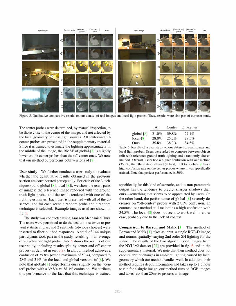
Figure 5. Qualitative comparative results on our dataset of real images and local light probes. These results were also part of our user study.

The center probes were determined, by manual inspection, to

be those close to the center of the image, and not affected by

the local geometry or close light sources. All center and off-

center probes are presented in the supplementary material.

Since it is trained to estimate the lighting approximately in

the middle of the image, the RMSE of global-[8] is slightly

lower on the center probes than the off-center ones. We note

that our method outperforms both versions of [8].

User study We further conduct a user study to evaluate

whether the quantitative results obtained in the previous

section are corroborated perceptually. For each of the 3 tech-

niques (ours, global-[8], local-[8]), we show the users pairs

of images: the reference image rendered with the ground

truth light probe, and the result rendered with one of the

lighting estimates. Each user is presented with all of the 20

scenes, and for each scene a random probe and a random

technique is selected. Example images used are shown in

fig. 5.

The study was conducted using Amazon Mechanical Turk.

The users were permitted to do the test at most twice to pre-

vent statistical bias, and 2 sentinels (obvious choices) were

inserted to filter out bad responses. A total of 144 unique

participants took part in the study, resulting in an average

of 20 votes per light probe. Tab. 5 shows the results of our

user study, including results split by center and off-center

probes (as defined in sec. 5.3). In all, our method achieves a

confusion of 35.8% (over a maximum of 50%), compared to

28% and 31% for the local and global versions of [8]. We

note that global-[8] outperforms ours slightly on the “cen-

ter” probes with a 39.8% vs 38.3% confusion. We attribute

this performance to the fact that this technique is trained

All Center Off-center

global-[8] 31.0% 39.8% 27.1%

local-[8] 28.0% 25.2% 29.5%

Ours 35.8% 38.3% 34.5%Table 5. Results of a user study on our dataset of real images and

local light probes. Users were asked to compare between objects

relit with reference ground truth lighting and a randomly chosen

method. Overall, users had a higher confusion with our method

(35.8%) than the state-of-the-art (at best, 31.0%). global-[8] has a

high confusion rate on the center probes where it was specifically

trained. Note that perfect performance is 50%.

specifically for this kind of scenario, and its non-parametric

output has the tendency to predict sharper shadows than

ours—something that seems to be appreciated by users. On

the other hand, the performance of global-[8] severely de-

creases on “off-center” probes with 27.1% confusion. In

contrast, our method still maintains a high confusion with

34.5%. The local-[8] does not seem to work well in either

case, probably due to the lack of context.

Comparison to Barron and Malik [1] The method of

Barron and Malik [1] takes as input, a single RGB-D image,

and returns spatially-varying 2nd order SH lighting for the

scene. The results of the two algorithms on images from

the NYU-v2 dataset [27] are provided in fig. 6 and in the

supplementary material. We note that their method does not

capture abrupt changes in ambient lighting caused by local

geometry which our method handles well. In addition, their

method requires depth information and takes up to 1.5 hour

to run for a single image; our method runs on RGB images

and takes less than 20ms to process an image.

6914

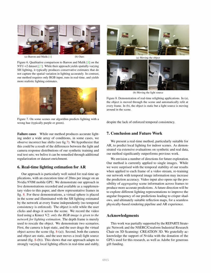
(a) Barron and Malik [1] (b) Ours

Figure 6. Qualitative comparison to Barron and Malik [1] on the

NYU-v2 dataset [27]. While their approach yields spatially-varying

SH lighting, it typically produces conservative estimates that do

not capture the spatial variation in lighting accurately. In contrast,

our method requires only RGB input, runs in real-time, and yields

more realistic lighting estimates.

Figure 7. On some scenes our algorithm predicts lighting with a

wrong hue (typically purple or green).

Failure cases While our method produces accurate light-

ing under a wide array of conditions, in some cases, we

observe incorrect hue shifts (see fig.7). We hypothesize that

this could be a result of the differences between the light and

camera response distributions of our synthetic training and

real test sets; we belive it can be remedied through additional

regularization or dataset enrichment.

6. Real-time lighting estimation for AR

Our approach is particularly well suited for real-time ap-

plications, with an execution time of 20ms per image on an

Nvidia 970M mobile GPU. We demonstrate our approach in

live demonstrations recorded and available as a supplemen-

tary video to this paper, and show representative frames in

fig. 8. For these demonstrations, a virtual sphere is placed

in the scene and illuminated with the SH lighting estimated

by the network at every frame independently (no temporal

consistency is enforced). The object is relit while the user

clicks and drags it across the scene. We record the video

feed using a Kinect V2: only the RGB image is given to the

network for lighting estimation. The depth frame is merely

used to rescale the object. We demonstrate two scenarios.

First, the camera is kept static, and the user drags the virtual

object across the scene (fig. 8-(a)). Second, both the camera

and object are static, and the user moves a (real) light source

around (fig. 8-(b)). This shows that our approach adapts to

strongly varying local lighting effects in real-time and stably,

(a) Moving the object

(b) Moving the light source

Figure 8. Demonstration of real-time relighting applications. In (a),

the object is moved through the scene and automatically relit at

every frame. In (b), the object is static but a light source is moving

around in the scene.

despite the lack of enforced temporal consistency.

7. Conclusion and Future Work

We present a real-time method, particularly suitable for

AR, to predict local lighting for indoor scenes. As demon-

strated via extensive evaluations on synthetic and real data,

our method significantly outperforms previous work.

We envision a number of directions for future exploration.

Our method is currently applied to single images. While

we were surprised with the temporal stability of our results

when applied to each frame of a video stream, re-training

our network with temporal image information may increase

the prediction accuracy. Video input also opens up the pos-

sibility of aggregating scene information across frames to

produce more accurate predictions. A future direction will be

to explore different lighting representations to improve the

angular frequency of our predictions leading to crisper shad-

ows, and ultimately suitable reflection maps, for a seamless

physically-based rendering pipeline and AR experience.

Acknowledgments

This work was partially supported by the REPARTI Strate-

gic Network and the NSERC/Creaform Industrial Research

Chair on 3D Scanning: CREATION 3D. We gratefully ac-

knowledge the support of Nvidia with the donation of the

GPUs used for this research, as well as Adobe for generous

gift funding.

6915

References

[1] J. Barron and J. Malik. Intrinsic scene properties from a

single rgb-d image. IEEE Conference on Computer Vision

and Pattern Recognition (CVPR), 2013.

[2] J. T. Barron and J. Malik. Shape, illumination, and reflectance

from shading. IEEE Transactions on Pattern Analysis and

Machine Intelligence (TPAMI), 37(8):1670–1687, 2015.

[3] V. Blanz and T. Vetter. A morphable model for the synthesis

of 3d faces. In ACM Transactions on Graphics (SIGGRAPH),

pages 187–194, 1999.

[4] D. Cheng, J. Shi, Y. Chen, X. Deng, and X. Zhang. Learning

scene illumination by pairwise photos from rear and front

mobile cameras. Computer Graphics Forum, 37:213–221, 10

2018.

[5] P. Debevec. Rendering synthetic objects into real scenes:

Bridging traditional and image-based graphics with global il-

lumination and high dynamic range photography. In Proceed-

ings of the 25th Annual Conference on Computer Graphics

and Interactive Techniques, ACM Transactions on Graphics

(SIGGRAPH), pages 189–198, 1998.

[6] P. E. Debevec and J. Malik. Recovering high dynamic range

radiance maps from photographs. In ACM Transactions on

Graphics (SIGGRAPH), page 31. ACM, 2008.

[7] Y. Ganin and V. Lempitsky. Unsupervised domain adaptation

by backpropagation. In International Conference on Machine

Learning (ICML), 2015.

[8] M.-A. Gardner, K. Sunkavalli, E. Yumer, X. Shen, E. Gam-

baretto, C. Gagne, and J.-F. Lalonde. Learning to predict

indoor illumination from a single image. ACM Transactions

on Graphics (SIGGRAPH Asia), 9(4), 2017.

[9] S. Georgoulis, K. Rematas, T. Ritschel, M. Fritz, T. Tuyte-

laars, and L. Van Gool. What is around the camera? In IEEE

International Conference on Computer Vision (ICCV), Oct

2017.

[10] S. Georgoulis, K. Rematas, T. Ritschel, E. Gavves, M. Fritz,

L. Van Gool, and T. Tuytelaars. Reflectance and natural

illumination from single-material specular objects using deep

learning. IEEE Transactions on Pattern Analysis and Machine

Intelligence (TPAMI), 40(8):1932–1947, 2018.

[11] R. Grosse, M. K. Johnson, E. H. Adelson, and W. T. Freeman.

Ground truth dataset and baseline evaluations for intrinsic

image algorithms. In IEEE International Conference on Com-

puter Vision (ICCV), 2009.

[12] L. Gruber, T. Richter-Trummer, and D. Schmalstieg. Real-

time photometric registration from arbitrary geometry. In

IEEE International Symposium on Mixed and Augmented

Reality (ISMAR). IEEE, 2012.

[13] Y. Hold-Geoffroy, A. Athawale, and J.-F. Lalonde. Deep

sky modeling for single image outdoor lighting estimation.

In IEEE International Conference on Computer Vision and

Pattern Recognition (CVPR), 2019.

[14] Y. Hold-Geoffroy, K. Sunkavalli, S. Hadap, E. Gambaretto,

and J.-F. Lalonde. Deep outdoor illumination estimation.

In IEEE International Conference on Computer Vision and

Pattern Recognition (CVPR), 2017.

[15] G. Huang, Z. Liu, L. van der Maaten, and K. Q. Weinberger.

Densely connected convolutional networks. In IEEE Confer-

ence on Computer Vision and Pattern Recognition (CVPR),

2017.

[16] F. N. Iandola, S. Han, M. W. Moskewicz, K. Ashraf, W. J.

Dally, and K. Keutzer. Squeezenet: Alexnet-level accuracy

with 50x fewer parameters and < 0.5 mb model size. arXiv

preprint arXiv:1602.07360, 2016.

[17] W. Jakob. Mitsuba renderer, 2010. http://www.mitsuba-

renderer.org.

[18] K. Karsch, V. Hedau, D. Forsyth, and D. Hoiem. Rendering

synthetic objects into legacy photographs. ACM Transactions

on Graphics (SIGGRAPH asia), 30(6):1, 2011.

[19] K. Karsch, K. Sunkavalli, S. Hadap, N. Carr, H. Jin, R. Fonte,

M. Sittig, and D. Forsyth. Automatic scene inference for 3d

object compositing. ACM Transactions on Graphics (SIG-

GRAPH), (3):32:1–32:15, 2014.

[20] E. A. Khan, E. Reinhard, R. W. Fleming, and H. H. Bulthoff.

Image-based material editing. ACM Transactions on Graphics

(SIGGRAPH), 25(3):654, 2006.

[21] J. F. Lalonde, A. A. Efros, and S. G. Narasimhan. Estimating

the natural illumination conditions from a single outdoor

image. International Journal of Computer Vision, 98(2):123–

145, 2012.

[22] J.-F. Lalonde, D. Hoiem, A. A. Efros, C. Rother, J. Winn, and

A. Criminisi. Photo clip art. ACM Transactions on Graphics

(SIGGRAPH), 26(3), July 2007.

[23] Z. Li and N. Snavely. CGIntrinsics: Better intrinsic image

decomposition through physically-based rendering. In Euro-

pean Conference on Computer Vision (ECCV), 2018.

[24] S. Lombardi and K. Nishino. Reflectance and illumination

recovery in the wild. IEEE Transactions on Pattern Analysis

and Machine Intelligence (TPAMI), 38(1), 2016.

[25] R. Maier, K. Kim, D. Cremers, J. Kautz, and M. Nießner. In-

trinsic3d: High-quality 3d reconstruction by joint appearance

and geometry optimization with spatially-varying lighting. In

Proceedings of the IEEE International Conference on Com-

puter Vision (ICCV), pages 3114–3122, 2017.

[26] R. Monroy, M. Hudon, and A. Smolic. Dynamic environ-

ment mapping for augmented reality applications on mobile

devices. In F. Beck, C. Dachsbacher, and F. Sadlo, editors,

Vision, Modeling and Visualization. The Eurographics Asso-

ciation, 2018.

[27] P. K. Nathan Silberman, Derek Hoiem and R. Fergus. Indoor

segmentation and support inference from rgbd images. In

European Conference on Computer Vision (ECCV), 2012.

[28] R. Ramamoorthi and P. Hanrahan. An efficient representation

for irradiance environment maps. In ACM Transactions on

Graphics (SIGGRAPH), pages 497–500. ACM, 2001.

[29] E. Reinhard, M. Stark, P. Shirley, and J. Ferwerda. Photo-

graphic tone reproduction for digital images. ACM transac-

tions on graphics (SIGGRAPH, 21(3):267–276, 2002.

[30] K. Rematas, T. Ritschel, M. Fritz, E. Gavves, and T. Tuyte-

laars. Deep reflectance maps. In IEEE Conference on Com-

puter Vision and Pattern Recognition (CVPR), 2016.

[31] O. Ronneberger, P. Fischer, and T. Brox. U-net: Convolutional

networks for biomedical image segmentation. In Interna-

tional Conference on Medical image computing and computer-

assisted intervention, pages 234–241. Springer, 2015.

6916

[32] P.-P. Sloan, J. Kautz, and J. Snyder. Precomputed radiance

transfer for real-time rendering in dynamic, low-frequency

lighting environments. In ACM Transactions on Graphics

(SIGGRAPH), volume 21, pages 527–536. ACM, 2002.

[33] S. Song, F. Yu, A. Zeng, A. X. Chang, M. Savva, and

T. Funkhouser. Semantic scene completion from a single

depth image. IEEE Conference on Computer Vision and

Pattern Recognition (CVPR), 2017.

[34] H. Weber, D. Prevost, and J.-F. Lalonde. Learning to estimate

indoor lighting from 3D objects. In International Conference

on 3D Vision (3DV), 2018.

[35] A. R. Zamir, A. Sax, W. Shen, L. Guibas, J. Malik, and

S. Savarese. Taskonomy: Disentangling task transfer learn-

ing. In IEEE Conference on Computer Vision and Pattern

Recognition (CVPR), 2018.

[36] E. Zhang, M. F. Cohen, and B. Curless. Emptying, refur-

nishing, and relighting indoor spaces. ACM Transactions on

Graphics (SIGGRAPH asia), 35(6), 2016.

[37] E. Zhang, M. F. Cohen, and B. Curless. Discovering point

lights with intensity distance fields. In IEEE Conference on

Computer Vision and Pattern Recognition (CVPR), 2018.

[38] Y. Zhang, S. Song, E. Yumer, M. Savva, J.-Y. Lee, H. Jin,

and T. Funkhouser. Physically-based rendering for indoor

scene understanding using convolutional neural networks.

The IEEE Conference on Computer Vision and Pattern Recog-

nition (CVPR), 2017.

6917