fast strong approximation monte-carlo schemes for ...kahl/publications/faststrong... · fast strong...

Fast strong approximation Monte-Carlo schemes forstochastic volatility models

Christian Kahl∗ Peter Jackel†

First version: 28th September 2005This version: 22nd May 2006

Abstract

Numerical integration methods for stochastic volatility models in financial markets are discussed.We concentrate on two classes of stochastic volatility models where the volatility is either directlygiven by a mean-reverting CEV process or as a transformed Ornstein-Uhlenbeck process. For thelatter, we introduce a new model based on a simple hyperbolic transformation. Various numericalmethods for integrating mean-reverting CEV processes are analysed and compared with respectto positivity preservation and efficiency. Moreover, we develop a simple and robust integrationscheme for the two-dimensional system using the strong convergence behaviour as an indicator forthe approximation quality. This method, which we refer to as the IJK (4.47) scheme, is applicableto all types of stochastic volatility models and can be employed as a drop-in replacement for thestandard log-Euler procedure.

Acknowledgment: The authors thank Vladimir Piterbarg and an anonymous referee for helpful com-ments and suggestions.

1 Introduction

Numerical integration schemes for differential equations have been around nearly as long as the formal-ism of calculus itself. In 1768, Euler devised his famous stepping method [Eul68], and this scheme hasremained the fallback procedure in many applications where all else fails as well as the benchmark interms of overall reliability and robustness any new algorithm must compete with. Many schemes havebeen invented since, and for most engineering purposes involving the numerical integration of ordinaryor partial differential equations there are nowadays a variety of approaches available.

With the advent of formal stochastic calculus in the 1920’s and the subsequent application to realworld problems came the need for numerical integration of dynamical equations subject to an externalforce of random nature. Again, Euler’s method came to the rescue, first suggested in this context byMaruyama [Mar55] whence it is also sometimes referred to as the Euler-Maruyama scheme [KP99].

An area where the calculus of stochastic differential equations became particularly popular is themathematics of financial markets, more specifically the modelling of financial movements for the pur-pose of pricing and risk-managing derivative contracts.

Most of the early applications of stochastic calculus to finance focussed on approaches that permit-ted closed form solutions, the most famous example probably being the Nobel prize winning article

∗Quantitative Analytics Group, ABN AMRO, 250 Bishopsgate, London EC2M 4AA, UK, and Department of Mathemat-ics, University of Wuppertal, Gaußstraße 20, Wuppertal, D-42119, Germany

†Global head of credit, hybrid, commodity, and inflation derivative analytics, ABN AMRO, 250 Bishopsgate, LondonEC2M 4AA, UK

1

by Fischer Black and Myron Scholes [BS73]. With increasing computer power, researchers and prac-titioners began to explore avenues that necessitated semi-analytical evaluations or even required fullynumerical treatment.

A particularly challenging modelling approach involves the coupling of two stochastic differentialequations whereby the diffusion term of the first equation is explicitly perturbed by the dynamics ofthe second equation: stochastic volatility models. These became of interest to financial practitionerswhen it was realised that in some markets deterministic volatility models do not represent the dynamicssufficiently. Alas, the first publications on stochastic volatility models [Sco87, Wig87, HW88] wereahead of their time: the required computer power to use these models in a simulation framework wassimply not available, and analytical solutions could not be found. One of the first articles that providedsemi-analytical solutions was published by Stein and Stein [SS91]. An unfortunate feature of that modelwas that it did not give enough flexibility to represent observable market prices, i.e. it did not provideenough degrees of freedom for calibration. In 1993, Heston [Hes93] published the first model thatallowed for a reasonable amount of calibration freedom permitting semi-analytical solutions. Variousother stochastic volatility models have been published since, and computer speed has increased signifi-cantly. However, despite the fact that at the time of this writing computer power makes fully numericaltreatment of stochastic volatility a real possibility, comparatively little research has been done on thesubject of efficient methods for the numerical integration of these models. In this article, we present anddiscuss some techniques that help to make the use of fully numerically integrated stochastic volatilitymodels a viable alternative to semi-analytic solutions, despite the fact that major advances on the effi-cient implementation of Heston’s model have been made [KJ05]. In section 2, we present the specificstochastic volatility models that we subsequently use in our demonstrations of numerical integrationmethods, and discuss some of their features in the context of financial markets modelling. In section 3,we elaborate on specific methods suitable for the volatility process in isolation. Next, in section 4, wediscuss techniques that accelerate the convergence of the numerical integration of the combined sys-tem of stochastic volatility and the directly observable financial market variable both with respect tothe discretisation refinement required and with respect to CPU time consumed. This is followed by thepresentation of numerical results in section 5. Finally, we conclude.

2 Some stochastic volatility models

We consider stochastic volatility models of the form

dSt = µStdt+ V pt StdWt (2.1)

where S describes the underlying financially observable variable and V , depending on the coefficient pgiven by the specific model, represents either instantaneous variance (p = 1/2) or instantaneous volatility(p = 1).

As for the specific processes for instantaneous variance or volatility, we distinguish two differentkinds. The first kind is the supposition of a given stochastic differential equation directly applied to theinstantaneous variance process. Since instantaneous variance must never be negative for the underlyingfinancial variable to remain on the real axis, we specifically focus on a process for variance of theform [Cox75, CR76, Bec80, AA00, CKLS92]

dVt = κ(θ − Vt)dt+ αV qt dZt, Vt0 = V0 . (2.2)

with κ, θ, α, q > 0, and p = 1/2 in equation (2.1). We assume the driving processes Wt and Zt to becorrelated Brownian motions satisfying dWt · dZt = ρ dt.

The second kind of stochastic volatility model we consider is given by a deterministic transformation

σt = σ0 · f(yt) , f : R → R+ , (2.3)

2

with f(·) being strictly monotonic and differentiable, of a standard Ornstein-Uhlenbeck process

dyt = −κytdt+ α√

2κ dZt, yt0 = y0 , (2.4)

setting Vt = σt and p = 1 in equation (2.1). The transformation f(·) is chosen to ensure that σ ≥ 0for the following reason. It is, in principle, possible to argue that instantaneous volatility is undefinedwith respect to its sign. However, when volatility and the process it is driving are correlated, a changeof sign in the volatility process implies a sudden change of sign in effective correlation, which in turnimplies a reversal of the conditional forward Black implied volatility skew, and the latter is a ratherundesirable feature to have for reasons of economic realism. As a consequence of this train of thought,we exclude the Stein & Stein / Schobel & Zhu model [SS91, SZ99] which is encompassed above bysetting f(y) = y.

In order to obtain a better understanding of the different ways to simulate the respective stochasticvolatility model we first give some analytical properties of the different approaches.

2.1 The mean-reverting CEV process

By mean-reverting CEV process we mean the family of processes described by the stochastic differentialequation (2.2). Heston’s model, for instance, is given by q = 1/2 with p = 1/2 in the process for theunderlying (2.1). The family of processes described by (2.2) has also been used for the modelling ofinterest rates [CKLS92].

For the special case q = 1/2, i.e. for the Heston variance process, the stochastic differential equationis also known as the Cox-Ingersoll-Ross model [CIR85]. In that case, the transition density is knownanalytically as

p(t0, t, Vt0 , Vt) = χ2d (νVt, ξ) (2.5)

with

ν =4κ

α2 (1− e−κ∆t)(2.6)

ξ =4κe−κ∆t

α2 (1− e−κ∆t)Vt0 (2.7)

∆t = t− t0 (2.8)

d =4θκ

α2(2.9)

where χ2d(x, ξ) denotes the noncentral chi-square density of variable x with d degrees of freedom and

non-centrality parameter ξ. Broadie and Kaya used this transition density for the Monte-Carlo simula-tion of European options [BK04].

With q = 1, equation (2.2) turns into a stochastic differential equation which is affine in the drift andlinear in the diffusion also known as the Brennan-Schwartz model [BS80]. To the best of our knowledge,there are no closed form explicit solutions for this equation allowing for a fully analytical expression,despite its apparent simplicity. A formal solution for equations of the form

dXt = (a1(t)Xt + a2(t)) dt+ (b1(t)Xt + b2(t)) dWt, Xt0 = X0 , (2.10)

is described in [KP99, Chap. 4.2 eq. (2.9)] as

Xt = Ξt0,t ·

X0 +

t∫t0

a2(s)− b1(s)b2(s)

Ξt0,s

ds+

t∫t0

b2(s)

Ξt0,s

dWs

(2.11)

with Ξt0,t given by [KP99, Chap. 4.2 eq. (2.7)]

Ξt0,t = eR t

t0(a1(s)− 1

2b21(s))ds+

R tt0

b1(s)dWs . (2.12)

3

Applying this to equation (2.2) with a1(t) = −κ, a2(t) = κθ, b1(t) = α and b2(t) = 0 leads to

Ξt0,t = e−(κ+ 12α2)(t−t0)+α(Wt−Wt0 ). (2.13)

as well as

Xt = e−“κ+α2

2

”t+αWt ·

X0 +

t∫t0

κθe“κ+α2

2

”s−αWsds

. (2.14)

The functional form of solution (2.14) is somewhat reminiscent of the payoff function of a continuouslymonitored Asian option in a standard Black-Scholes framework, and thus it may be possible to derivethe Laplace transform of the distribution of Xt analytically following the lead given by Geman andYor [GY93]. However, whilst this is noteworthy in its own right, it is unlikely to aid in the develop-ment of fast and efficient numerical integration schemes for Monte Carlo simulations, especially if theultimate aim is to use the process X to drive the diffusion coefficient in a second stochastic differentialequation.

Beyond the cases q = 0, q = 1/2, and q = 1, as far as we know, there are no analytical or semi-analytical solutions. Nevertheless, we are able to discuss the boundary behaviour solely based on ourknowledge of the drift and diffusion terms:

1. 0 is an attainable boundary for 0 < q < 1/2 and for q = 1/2 if κθ < α2/2

2. 0 is unattainable for q > 1/2

3. ∞ is unattainable for all q > 0.

These statements can be confirmed by the aid of Feller’s boundary classification which can be foundin [KT81]. The stationary distribution of this process can be calculated as (see [AP04, Prop. 2.4])

π(y) = C(q)−1y−2qeM(y,q), C(q) =

∞∫0

y−2qeM(y,q)dy (2.15)

with the auxiliary function M(y, q) given by

1. q = 1/2

M(y, q) =2κ

α2(θ ln(y)− y) (2.16)

2. q = 1

M(y, q) =2κ

α2(−θ/y − ln(y)) (2.17)

3. 0 < q < 1/2 and 1/2 < q < 1

M(y, q) =2κ

α2

(θy1−2q

1− 2q− y2−2q

2− 2q

). (2.18)

The above equations can be derived from the Fokker-Planck equation which leads to an ordinary differ-ential equation of Bernoulli type. The first moment of the process (2.2) is given by

E[Vt] = (Vt0 − θ)e−κt + θ . (2.19)

We can also calculate the second moment for q = 1/2 or q = 1 :

E[V 2

t

]=

e−2κt(eκt−1)(2V0+(eκt−1)θ)(α2+2θκ)

2κfor q = 1/2

2e−2κtθκ“

e2κtθ(κ−α2)+eκt(V0−θ)(2κ−α2)+eα2t(V0(α2−2κ)+θκ)”

α4−3α2κ+2κ2 for q = 1 .(2.20)

4

This means that in the case q = 1, for α2 > κ which is typically required in order to calibrate to themarket observable strongly pronounced implied-Black-volatility skew, the variance of volatility growsunbounded, despite the fact that the model appears to be mean-reverting. For long dated options, this isa rather undesirable feature to have. On the other hand, in the case q = 1/2, for α2 > κ, instantaneousvariance can attain zero, which is also undesirable for economical reasons. In addition to that, forthe modelling of path dependent derivatives, the model (2.2) requires the use of numerical integrationschemes that preserve the analytical properties of the variance process such as to remain on the real axis,or to simply stay positive. In the next section, we discuss alternatives for the generation of the stochasticvolatility process that make the integration of volatility itself practically trivial.

2.2 Transformed Ornstein-Uhlenbeck

The origin of this process goes back to Uhlenbeck and Ornstein’s publication [UO30] in which theydescribe the velocity of a particle that moves in an environment with friction. Doob [Doo42] firsttreated this process purely mathematically and expressed it in terms of a stochastic differential equation.In modern financial mathematics, the use of Ornstein-Uhlenbeck processes is almost commonplace.The attractive features of an Ornstein-Uhlenbeck process are that, whilst it provides a certain degree offlexibility over its auto-correlation structure, it still allows for the full analytical treatment of a standardGaussian process.

In this article, we chose the formulation (2.4) to describe the Ornstein-Uhlenbeck process since weprefer a parametrisation that permits complete separation between the mean reversion speed and thevariance of the limiting or stationary distribution of the process. The solution of (2.4) is

Yt = e−κt

y0 +

t∫0

eκuα√

2κ dZu

(2.21)

with initial time t0 = 0. In other words, the stochastic process at time t is Gaussian with

Yt ∼ N(y0e−κt, α2

(1− e−2κt

))(2.22)

and thus the stationary distribution is Gaussian with variance α2: a change in parameter κ requires norescaling of α if we wish to hold the long-term uncertainty in the process unchanged. It is straightfor-ward to extend the above results to the case when κ(t) and α(t) are functions of time [Jac02]. Since thevariance of the driving Ornstein-Uhlenbeck process is the main criterion that determines the uncertaintyin volatility for the financial underlying process, all further considerations are primarily expressed interms of

η(t) := α ·√

1− e−2κt . (2.23)

There are fundamental differences between the requirements in the financial modelling of underlyingasset prices, and the modelling of instantaneous stochastic volatility, or indeed any other not directlymarket-observable quantity. For reasons of financial consistency, we frequently have to abide by no-arbitrage rules that impose a specific functional form for the instantaneous drift of the underlying. Incontrast, the modelling of stochastic volatility is typically more governed by long-term realism andstructural similarity to real-world dynamics, and no externally given drift conditions apply. No-arbitragearguments and their implied instantaneous drift conditions are omnipresent in financial arguments, andas a consequence, most practitioners have become used to thinking of stochastic processes exclusivelyin terms of an explicit stochastic differential equation. However, when there are no explicitly givenconditions on the instantaneous drift, it is, in fact, preferable to model a stochastic process in the mostanalytically convenient form available. In other words, when preferences as to the attainable domainof the process are to be considered, it is in practice much more intuitive to start with a simple processof full analytical tractability, and to transform its domain to the target domain by virtue of a simpleanalytical function. For the modelling of stochastic volatility, this means that we utilise the flexible yet

5

tractable nature of the Ornstein-Uhlenbeck process (2.4) in combination with a strictly monotonic anddifferentiable mapping function f : R → R+.

One simple analytical transformation we consider is the exponential function, and the resultingstochastic volatility model was first proposed in [Sco87, equation (7)]. The model is intuitively veryappealing: for any future point in time, volatility has a lognormal distribution which is a very comfort-able distribution for practitioners in financial mathematics. Alas, though, recent research [AP04] hascast a shadow on this model’s analytical features. It appears that, in its full continuous formulation, thelog-normal volatility model can give rise to unlimited higher moments of the underlying financial asset.However, as has been discussed and demonstrated at great length for the very similar phenomenon of in-finite futures returns when short rates are driven by a lognormal process [HW93, SS94, SS97a, SS97b],this problem vanishes as soon as the continuous process model is replaced by its discretised approx-imation which is why lognormal volatility models remain numerically tractable in applications. Still,in order to avoid this problem altogether, we introduce an alternative to the exponential transformationfunction which is given by a simple hyperbolic form.

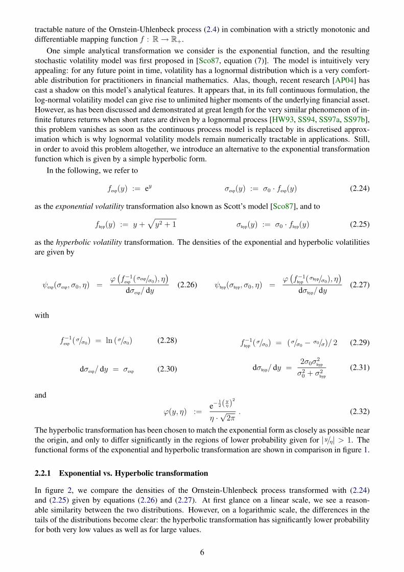
In the following, we refer to

fexp(y) := ey σexp(y) := σ0 · fexp(y) (2.24)

as the exponential volatility transformation also known as Scott’s model [Sco87], and to

fhyp(y) := y +√y2 + 1 σhyp(y) := σ0 · fhyp(y) (2.25)

as the hyperbolic volatility transformation. The densities of the exponential and hyperbolic volatilitiesare given by

ψexp(σexp, σ0, η) =ϕ(f−1

exp (σexp/σ0), η)

dσexp/ dy(2.26) ψhyp(σhyp, σ0, η) =

ϕ(f−1

hyp (σhyp/σ0), η)

dσhyp/ dy(2.27)

with

f−1exp (σ/σ0) = ln (σ/σ0) (2.28) f−1

hyp (σ/σ0) = (σ/σ0 − σ0/σ)/ 2 (2.29)

dσexp/ dy = σexp (2.30) dσhyp/ dy =2σ0σ

2hyp

σ20 + σ2

hyp

(2.31)

and

ϕ(y, η) :=e−

12(

yη )

2

η ·√

2π. (2.32)

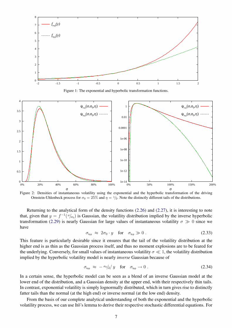
The hyperbolic transformation has been chosen to match the exponential form as closely as possible nearthe origin, and only to differ significantly in the regions of lower probability given for |y/η| > 1. Thefunctional forms of the exponential and hyperbolic transformation are shown in comparison in figure 1.

2.2.1 Exponential vs. Hyperbolic transformation

In figure 2, we compare the densities of the Ornstein-Uhlenbeck process transformed with (2.24)and (2.25) given by equations (2.26) and (2.27). At first glance on a linear scale, we see a reason-able similarity between the two distributions. However, on a logarithmic scale, the differences in thetails of the distributions become clear: the hyperbolic transformation has significantly lower probabilityfor both very low values as well as for large values.

6

0

1

2

3

4

5

6

7

8

-2 -1.5 -1 -0.5 0 0.5 1 1.5 2

fexp(y)

fhyp(y)

Figure 1: The exponential and hyperbolic transformation functions.

0

0.5

1

1.5

2

2.5

3

3.5

4

0% 20% 40% 60% 80% 100%

σ

ψexp(σ,σ0,η)

ψhyp(σ,σ0,η)

1e-14

1e-12

1e-10

1e-08

1e-06

0.0001

0.01

1

0% 50% 100% 150% 200%

σ

ψexp(σ,σ0,η)

ψhyp(σ,σ0,η)

Figure 2: Densities of instantaneous volatility using the exponential and the hyperbolic transformation of the drivingOrnstein-Uhlenbeck process for σ0 = 25% and η = 1/2. Note the distinctly different tails of the distributions.

Returning to the analytical form of the density functions (2.26) and (2.27), it is interesting to notethat, given that y = f−1(σ/σ0) is Gaussian, the volatility distribution implied by the inverse hyperbolictransformation (2.29) is nearly Gaussian for large values of instantaneous volatility σ � 0 since wehave

σhyp ≈ 2σ0 · y for σhyp � 0 . (2.33)

This feature is particularly desirable since it ensures that the tail of the volatility distribution at thehigher end is as thin as the Gaussian process itself, and thus no moment explosions are to be feared forthe underlying. Conversely, for small values of instantaneous volatility σ � 1, the volatility distributionimplied by the hyperbolic volatility model is nearly inverse Gaussian because of

σhyp ≈ − σ0/2/ y for σhyp → 0 . (2.34)

In a certain sense, the hyperbolic model can be seen as a blend of an inverse Gaussian model at thelower end of the distribution, and a Gaussian density at the upper end, with their respectively thin tails.In contrast, exponential volatility is simply lognormally distributed, which in turn gives rise to distinctlyfatter tails than the normal (at the high end) or inverse normal (at the low end) density.

From the basis of our complete analytical understanding of both the exponential and the hyperbolicvolatility process, we can use Ito’s lemma to derive their respective stochastic differential equations. For

7

the exponential transformation (2.24) we obtain Scott’s original SDE [Sco87, equation (7)]

dσ = κσ(α2 − ln(σ/σ0)

)dt+ ασ

√2κ dZ . (2.35)

It is remarkable to see the difference in the stochastic differential equation we obtain for the hyperbolicvolatility process (2.25):

dσ = −κσσ6 + σ4σ2

0 − (8α2 + 1)σ2σ40 − σ6

0

(σ2 + σ20)

3 dt + σα√

8κσσ0

σ2 + σ20

dZ . (2.36)

The complexity of the explicit form (2.36) of the hyperbolic volatility process may help to explainwhy it has, to the best of our knowledge, not been considered before. As we know, though, the re-sulting process is of remarkable simplicity and very easy to simulate directly, whilst overcoming someof the weaknesses of the (calibrated) CIR/Heston process (namely that zero is attainable), as well asthe moment divergence when volatility or variance is driven by lognormal volatility as incurred by theBrennan-Schwartz process for volatility and Scott’s model.

The moments of the exponential transformation function are

E[(fexp(y))m] = e

12m2η2

. (2.37)

For the hyperbolic transformation we obtain the general solution

E[(fhyp(y))m] = 2

32 n

√4πηnΓ

(1+n

2

)1F1(−n

2, 1− n, 1

2η2 ) + 2−32 n

√4πη−nΓ

(1−n

2

)1F1(

n2, 1 + n, 1

2η2 ) (2.38)

in terms of Kummer’s hypergeometric function 1F1. The first two moments, specifically, are given by

E[(fhyp(y))

1] =√

2 · η · U(−12, 0, 1

2η2 ) (2.39)

E[(fhyp(y))

2] = 1 + 2η2 (2.40)

where U(a, b, z) is the logarithmic confluent hypergeometric function. More revealing than the closedform for the moments of the respective transformation functions is an analysis based on their Taylorexpansions

fexp(y) = 1 + y +y2

2+O

(y3)

(2.41)

fhyp(y) = 1 + y +y2

2+O

(y4). (2.42)

Thus, for both of these functions,

(f···(y))n = 1 + n · y +

[(n

2

)+n

2

]· y2 +O

(y3). (2.43)

Since y is normally distributed with mean 0 and variance η2, and since all odd moments of the Gaussiandistribution vanish, this means that for both the exponential and the hyperbolic transformation we have

E[(f···(y))n] = 1 +

[(n

2

)+n

2

]· η2 +O

(η4). (2.44)

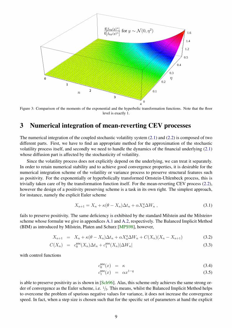
The implication of (2.44) is that all moments of the exponential and the hyperbolic transformationfunction agree up to orderO (η3). We show an example for this in figure 3. As η increases, the momentsof the exponential function grow faster by a term of order O (η4).

8

n

η

E[fexp(y)n]

E[fhyp(y)n]for y ∼ N (0, η2)

0

1

2

3

40

0.1

0.2

0.3

0.4

0.5

1.2

1.4

1.6

0

1

2

3

1.2

Figure 3: Comparison of the moments of the exponential and the hyperbolic transformation functions. Note that the floorlevel is exactly 1.

3 Numerical integration of mean-reverting CEV processes

The numerical integration of the coupled stochastic volatility system (2.1) and (2.2) is composed of twodifferent parts. First, we have to find an appropriate method for the approximation of the stochasticvolatility process itself, and secondly we need to handle the dynamics of the financial underlying (2.1)whose diffusion part is affected by the stochasticity of volatility.

Since the volatility process does not explicitly depend on the underlying, we can treat it separately.In order to retain numerical stability and to achieve good convergence properties, it is desirable for thenumerical integration scheme of the volatility or variance process to preserve structural features suchas positivity. For the exponentially or hyperbolically transformed Ornstein-Uhlenbeck process, this istrivially taken care of by the transformation function itself. For the mean-reverting CEV process (2.2),however the design of a positivity preserving scheme is a task in its own right. The simplest approach,for instance, namely the explicit Euler scheme

Xn+1 = Xn + κ(θ −Xn)∆tn + αXqn∆Wn , (3.1)

fails to preserve positivity. The same deficiency is exhibited by the standard Milstein and the Milstein+scheme whose formulæ we give in appendices A.1 and A.2, respectively. The Balanced Implicit Method(BIM) as introduced by Milstein, Platen and Schurz [MPS98], however,

Xn+1 = Xn + κ(θ −Xn)∆tn + αXqn∆Wn + C(Xn)(Xn −Xn+1) (3.2)

C(Xn) = cBIM0 (Xn)∆tn + cBIM

1 (Xn)|∆Wn| (3.3)

with control functions

cBIM0 (x) = κ (3.4)cBIM1 (x) = αx1−q (3.5)

is able to preserve positivity as is shown in [Sch96]. Alas, this scheme only achieves the same strong or-der of convergence as the Euler scheme, i.e. 1/2. This means, whilst the Balanced Implicit Method helpsto overcome the problem of spurious negative values for variance, it does not increase the convergencespeed. In fact, when a step size is chosen such that for the specific set of parameters at hand the explicit

9

Euler scheme is usable1, the Balanced Implicit Method often has worse convergence properties than theexplicit Euler method. This feature of the Balanced Implicit Method is typically caused by the fact thatthe use of the weight function cBIM

1 effectively increases the unknown coefficient dominating the leadingerror terms.

Another scheme that has been shown to preserve positivity for certain parameter ranges is the adap-tive Milstein scheme [Kah04] with suitable stepsize ∆τn and z ∼ N (0, 1)

Xn+1 = Xn + κ(θ −Xn)∆τn + αXqn

√∆τnz +

1

2α2qX2q−1

n ∆τn(z 2 − 1

). (3.6)

Unfortunately, this scheme requires adaptive resampling and thus necessitates the use of a pseudo-random number pipeline which in turn disables or hinders a whole host of independently availableconvergence enhancement techniques such as low-discrepancy numbers, importance sampling, strati-fication, latin-hypercube methods, etc. An advanced method that obviates the use of pseudo-randomnumber pipelines is based on the combination of the Milstein scheme with the idea of balancing: theBalanced Milstein Method (BMM)

Xn+1 = Xn + κ(θ −Xn)∆tn + αXqn∆Wn +

1

2α2qX2q−1

n

(∆W 2

n −∆tn)

(3.7)

+D(Xn) (Xn −Xn+1) ,

D(Xn) = dBMM0 (Xn)∆tn + dBMM

1 (Xn)(∆W 2

n −∆tn). (3.8)

As in the Balanced Implicit Method we can control the integration steps by using weighting functionsdBMM

0 (·) and dBMM1 (·). The choice of these weighting functions strongly depends on the structure of the

SDE. It can be shown (see [KS05, Theorem 5.9]) that the BMM preserves positivity for the mean-reverting CEV model (2.2) with the following choice

dBMM0 (x) = Θκ+

1

2α2q|x|2q−2 , (3.9)

dBMM1 (x) = 0 . (3.10)

The parameter Θ ∈ [0, 1] provides some freedom for improved convergence speed but it has to be chosensuch that

∆tn <2q − 1

2qκ(1−Θ). (3.11)

It is always safe to choose Θ = 1, though, for improved performance, we used Θ = 1/2 whenever thischoice was possible2.

The above mentioned integration methods, namely the standard explicit Euler scheme, the Bal-anced Implicit Method, the Balanced Milstein Method, and the adaptive Milstein scheme, deal withthe stochastic differential equation in its original form (2.2). Another approach to integrate (2.2) whilstpreserving positivity is to transform the stochastic differential equation to logarithmic coordinates us-ing Ito’s lemma as suggested by Andersen and Brotherton-Ratcliffe [ABR01]. Applying this to themean-reverting CEV process leads to

d lnVt =2κ(θ − Vt)− α2V 2q−1

t

2Vt

dt+ αV q−1t dZt (3.12)

which can be solved by the aid of a simple Euler scheme. The major drawback with this approach isthat, whilst the Euler scheme applied to the transformed stochastic differential equation (3.12) preserves

1For most schemes, spurious negative values incurred as an undesirable side effect of the numerical method disappear asthe step size ∆t is decreased. For a negative variance to appear at any one step, the drawn normal variate generating the steptypically has to exceed a certain threshold. This threshold tends to grow as step size decreases. Thus, with decreasing stepsize, eventually, the threshold exceeds the maximum standard normal random number attainable on the finite representationcomputer system used.

2For q = 1/2 the numerator becomes zero. Despite this, positivity can be preserved with dBMM0 = κ.

10

positivity, it is also likely to become unstable for suitable time steps [ABR01]. These instabilities are adirect consequence of the divergence of both the drift and the diffusion terms near zero. For that reasonAndersen and Brotherton-Ratcliffe suggested a moment matched log-normal approximation

Vn+1 =(θ + (Vn − θ) e−κ∆tn

)e−

12Γ2

n+Γnz , (3.13)

Γn = ln

(1 +

12α2V 2p

n κ−1(1− e−2κ∆tn

)(θ + (Vn − θ) e−κ∆tn)2

)(3.14)

with z ∼ N (0, 1). We will refer to this integration scheme as moment matched Log-Euler in thefollowing. This method is at its most effective for the Brennan-Schwartz model (3.23) as we can seein figure 7 (B) since for p = 1 the logarithmic transformation leads to an additive diffusion (3.12)term. However, even in that case, it is outperformed by the bespoke method we call Pathwise AdaptedLinearisation which is explained in section 3.1, as well as the Balanced Milstein method (3.7). For theHeston case, where the stochastic volatility is given by the Cox-Ingersoll-Ross equation with q = 1/2which is shown in figures 5 and 6, the moment matched log-Euler method has practically no convergenceadvantage over straightforward explicit Euler integration as long as the size of α is reasonably small.Contrarily, the approximation quality of all integration schemes is decisively reduced when dealingwith large α as we can see in figure 5 (B). Making matters even worse, one can observe that schemesof Milstein type are losing their strong convergence order of 1. The explanation for this behaviour israther simple: the Milstein method is not even guaranteed to converge at all for the mean-revertingCEV process (2.2)! Having a closer look at the diffusion b(x) = αxq, we recognize that for q < 1this function is not continuously differentiable on R which is necessary for the application of stochasticTaylor expansion techniques. Nonetheless, as long as the stochastic process is analytically positive, i.e.x > 0 there exists a local stochastic Taylor expansion preserving strong convergence of the Milsteinmethod. However, when zero is attainable, the discontinuity of the first derivative of the diffusion b(x)reduces the strong convergence order to 1/2.

In figures 5, 6, and 7 we present examples for the convergence behaviour of the different methods incomparison. For the standard Milstein (A.5) and the Milstein+ scheme (A.15), for some of the parameterconfigurations, it was necessary to floor the simulated variance values at zero since those schemes donot preserve positivity by construction.

The depicted strong approximation convergence measure is given by the L2 norm of the differencebetween the simulated terminal value, and the terminal value of the reference calculation, averaged overall M paths, i.e. √√√√ 1

M

M∑i=1

(X

(nsteps)i (T )−X

(nreference)i (T )

)2

. (3.15)

This quantity is shown as a function of average CPU time per path. This was done because the ulti-mate criterion for the choice of any integration method in applications is the cost of accuracy in termsof calculation time since calculation time directly translates into the amount of required hardware forlarge scale computations such as overnight risk reports, or into user downtime when interactive valua-tions are needed. This does, of course, make the results dependent on the used hardware3, not only inabsolute terms but also in relative terms since different processor models require different numbers ofCPU clock cycles for all the involved basic floating point operations. Nevertheless, the pathwise erroras a function of average CPU time is probably the most significant criterion for the quality of any inte-gration method. Examples for this consideration are the fact that in figure 6 the nominal advantage ofthe moment matched Log-Euler is almost precisely offset by the additional calculation time it requirescompared to the Euler scheme, and also that in figure 7 (B) the relative performance of the BalancedMilstein Method is compatible with the scheme denoted as Pathwise Adapted Linearisation which isexplained in section 3.1.1.

3Throughout this article, all calculations shown were carried out on a processor from the Intel Pentium series (Family 6,Model 9, Stepping 5, Brand id 6, CPU frequency 1700 MHz).

11

The curves in figures 5, 6 and 7 have been constructed by repeated simulation with increased num-bers of steps in the Brownian bridge Wiener path generation in powers of two from 1 to 128:

nsteps ∈ {1, 2, 4, 8, 16, 32, 64, 128} . (3.16)

The reference solution was always computed with 215 steps. The number generation mechanism usedwas the Sobol’ algorithm [Jac02] throughout apart from figure 6 (B) where we also show the resultsfrom using the Mersenne Twister [MN98] in comparison. Note that the results are fairly insensitiveto the choice of number generator. In addition to the methods discussed above, we also included theresults from bespoke schemes denoted as Pathwise Adapted Linearisation. These schemes are carefullyadapted to the respective equation and we introduce them in the following section.

3.1 Pathwise approximations for specific cases

Yet another approach for the numerical integration of stochastic differential equations of the form

dX = a(X)dt+ b(X)dZ (3.17)

as it is the case for (2.2) is to apply Doss’s [Dos77] method of constructing pathwise solutions first usedin the context of numerical integration schemes by Pardoux and Talay [PT85]. The formal derivation ofDoss’s pathwise solution can be found in [KS91, pages 295–296].

In practice, Doss’s method can hardly ever be applied directly since it is essentially just an exis-tence theorem that states that any process for which there is a unique strong solution can be seen as atransformation of the solution to an ordinary differential equation with a stochastic inhomogeneity, i.e.a solution of the form

X = f(Y, Z) with boundary condition f(Y, Z0) = Y (3.18)

withdY = g(Y, Z)dt (3.19)

implyingX0 = Y0 (3.20)

whereby the functions f and g can be derived constructively from the stochastic differential equationfor X:

∂Y f(Y, Z) = eR Z

Z0b′(f(y,z)) dz (3.21)

g(Y, Z) =

[a (f(Y, Z))− 1

2· b (f(Y, Z)) · b′ (f(Y, Z))

]· e−

R ZZ0

b′(f(Y,z)) dz. (3.22)

Even though one can rarely use Doss’s method in its full analyticity, one can often devise a powerfulbespoke approximate discretisation scheme for the stochastic differential equation at hand based onDoss’s pathwise existence theorem by the aid of some simple approximative assumptions without theneed to go through the Doss formalism itself.

3.1.1 Pathwise approximation of the Brennan-Schwartz SDE

For q = 1, the mean-reverting CEV process (2.2) becomes

dX = κ(θ −X)dt+ αXdZ . (3.23)

Assumingκ > 0 , θ > 0 , α > 0 , and X(0) > 0 , (3.24)

12

we must haveXt ≥ 0 for all t > 0 . (3.25)

Using equation (3.21), we obtainf(Y, Z) = Y eαZ . (3.26)

and by the aid of (3.22), we have

dY =

[κθe−αZ −

(κ+

1

2α2

)Y

]dt . (3.27)

We cannot solve this equation directly. Also, a directly applied explicit Euler scheme would permit Y tocross over to the negative half of the real axis and thus X = f(Y, Z) = Y eαZ would leave the domainof (3.23). What’s more, an explicit Euler scheme applied to equation (3.27) would mean that, within thescheme, we interpret Zt as a piecewise constant function. Not surprisingly, it turns out below that wecan do better than that!

Recall that, for the given time discretisation, we explicitly construct the Wiener process values Z(ti)and thus, for the purpose of numerical integration of equation (3.23), they are known along any onegiven path. If we now approximate Zt as a piecewise linear function in between the known values at tnand tn+1, i.e.

Zt ≈ βnt+ γn for t ∈ [tn, tn+1] (3.28)

with

γn = Z(tn)− βntn and βn =Z(tn+1)− Z(tn)

tn+1 − tn, (3.29)

then we have the approximating ordinary differential equation

dY =[κθe−α(βnt+γn) −

(κ+ 1

2α2)Y]

dt . (3.30)

Using the abbreviations

δn := κ+ 12α2 − αβn , ∆tn := tn+1 − tn , and Zn+1 := Z(tn+1)

we can write the solution to equation (3.30) as

Yn+1 = Yne−(κ+ 12α2)∆tn + κθ · e−αZn+1 ·

(1− e−δn∆tn

δn

), (3.31)

which gives us

Xn+1 = Xne−δn∆tn + κθ ·(

1− e−δn∆tn

δn

). (3.32)

This scheme is unconditionally stable. We refer to it as Pathwise Adapted Linearisation in the following.Apart from its stability, this scheme has the additional desirable property that, in the limits θ → 0 and/orκ → 0, i.e. in the limit of equation (3.23) resembling a standard geometric Brownian motion, it is freeof any approximation. Since in practice θ and/or κ tend to be not too large, the scheme’s proximity toexactness translates into a remarkable acccuracy when used in applications.

It is interesting to note that a similar approach based on replacing the term dZ directly in the stochas-tic differential equation

dX = κ(θ −X)dt+ αXdZ (3.33)

by a linear approximation dZ ≈ βdt gives rise to a scheme that does not converge in the limit ∆t→ 0 asfirst observed by Wong and Zakai [WZ65]. However, if we make the same replacement in the Milsteinscheme and drop terms of order O(dt2) and higher, which for (3.23) means

∆X ≈ κ(θ −X)∆t+ αX∆Z +1

2α2X

(∆Z2 −∆t

)(3.34)

∆X ≈ κ(θ −X)∆t+ αXβ∆t+1

2α2X

(β2∆t2 −∆t

)(3.35)

dXdt

≈ κ(θ −X)− 1

2α2X + αβX , (3.36)

13

and integrate, we arrive at exactly the same scheme (3.32) as if we had gone through the full Dossformalism. The reason for this is that the lowest order scheme that includes explicitly all terms thatare individually in expectation of order dt is the Milstein scheme, not the Euler scheme, and the differ-ence terms are crucial to preserve strong convergence when we introduce piecewise linearisation of thediscretised Wiener process.

3.1.2 Pathwise approximation of the Cox-Ingersoll-Ross / Heston SDE

The special case q = 1/2 of (2.2) represents the stochastic differential equation of the variance processin the Heston model [Hes93], as well as the short rate process in the Cox-Ingersoll-Ross model [CIR85]

dV = κ(θ − V )dt+ α√V dZ . (3.37)

In this case, an explicit solution of the Doss formalism (3.21) is not obvious. However, by conditioningon one specific path in Z we can bypass this difficulty by directly approximating Zt as a piecewiselinear function in between the known values as given in equations (3.28) and (3.29). Using the resultingdependency dZ = βndt in the Milstein scheme applied to (3.37)

dV ≈ κ(θ − V )dt+ α√V dZ +

1

4α2(dZ2 − dt

), (3.38)

i.e.dV ≈ κ(θ − V )dt+ α

√V βndt+

1

4α2(β2

ndt2 − dt), (3.39)

and dropping terms of order dt2, we obtain the approximate ordinary differential equation

dVdt

≈ κ(θ − V )− 1

4α2 + αβn

√V (3.40)

which has the implicit solution

t− tn = T (Vt, βn)− T (Vtn , βn) (3.41)

with

T (v, β) := 2αβ

κ√

α2β2+4θκ2−κα2atanh

(2κ√

v−αβ√α2β2+4θκ2−κα2

)− 1

κln

(κ (v − θ) +

1

4α2 − αβ

√v

).

(3.42)Equation (3.42) can be solved numerically comparatively readily since we know that, given βn, over thetime step from tn to tn+1, Vt will move monotonically, and that for all ∆tn := (tn+1 − tn) we have

Vtn+1 >

α |βn|2κ

−

√(αβn

2κ

)2

+ θ − α2

4κ

2

(3.43)

which can be shown by setting the argument of the logarithm in the right hand side of equation (3.42)to zero. Alternatively, an inverse series expansion can be derived. Up to order O(∆t4n), we find

Vn+1 = Vn +(κ(θ − Vn) + αβn

√Vn

)·∆tn·

·

[1 + αβn−2κ

√Vn

4√

Vn·∆tn +

κ(Vn(4κ√

Vn−3αβn)−αβnθ)24√

Vn3 ·∆t2n (3.44)

+κ(3αβnκθ2+κV 2

n (7αβn−8κ√

Vn)+2αβnθ√

Vn(αβn+κ√

Vn))192

√Vn

5 ·∆t3n

]+O(∆t5n)

14

with

θ := θ − α2

4κ. (3.45)

The shape of the curves generated by (3.42) and its 4th order inverse expansion (3.44) is shown in figure 4where values for β directly represent the standard normal deviation equivalent of the drawn Gaussianrandom number. In the following, we denoted the expansion (3.44) as Pathwise Adapted LinearisationQuartic, and its second order truncation

Vn+1 = Vn +(κ(θ − Vn) + αβn

√Vn

)·∆tn ·

[1 + αβn−2κ

√Vn

4√

Vn·∆tn

]+O(∆t3n) (3.46)

as Pathwise Adapted Linearisation Quadratic. We only show results for expansions of even order forreasons of numerical stability since all odd order expansion can reach zero which is undesirable. Forsmall values of α as in figure 5 (A) both schemes are remarkable effective. Unfortunately, these schemesare inappropriate for large values of α due to numerical instabilities.

0%

5%

10%

15%

20%

25%

30%

35%

40%

45%

0 0.2 0.4 0.6 0.8 1

σ (t

)

t

β = 3

4th order expansion for β = 3

β = 2


β = 1


β = 0


β = -1

4th order expansion for β = -1

β = -2


β = -3


Figure 4: Approximation (3.42) and its quartic expansion (3.44) for the CIR/Heston volatility process for σ(0) =√

V (0) =20%, θ = V (0), α = 20%, κ = 1 over a unit time step for different levels of the variate β = Z(1)− Z(0).

4 Approximation of stochastic volatility models

In this section, we discuss the numerical treatment of the full two-dimensional stochastic volatilitymodel. Irrespective of the volatility or variance process, the dynamics of the financial underlying aregiven by equation (2.1). As for the stochasticity of volatility/variance, both the transformed Ornstein-Uhlenbeck process as well as the mean-reverting CEV process (2.2) can be cast in the form

dVt = a(Vt)dt+ b(Vt)dZt . (4.1)

For the mean-reverting CEV process, the functional forms for a and b are directly given. For the expo-nentially and hyperbolically transformed Ornstein-Uhlenbeck process, they can be obtained from (2.35)and (2.36), respectively.

In logarithmic coordinates, the process equation for the financial underlying is given by

lnSt = lnSt0 +

t∫t0

µ(s)ds− 12

t∫t0

V 2ps ds+

t∫t0

V ps dWs . (4.2)

15

(A)

0.0001

0.001

0.01

1 10 100

Euler

Milstein

Milstein+

Balanced Implicit Method

Balanced Milstein Method

Moment matched log-Euler

Pathwise Adapted Linearisation Quadratic

Pathwise Adapted Linearisation Quartic

(B)

0.01

0.1

1 10 100

Euler

Milstein

Milstein+





Figure 5: Strong convergence measured by expression (3.15) as a function of CPU time [in msec] averaged over 32767 pathsfor the mean reverting CEV model (2.2) for q = 1/2, κ = 1, V0 = θ = 1/16, T = 1, cBIM

0 = 1, cBIM1 = α/

√x, dBMM

0 = κ,dBMM1 = 0. The number generator was the Sobol’ method. (A): α = 0.2, α2 − 2κθ = −0.085; zero is unattainable. (B):

α = 0.8, α2 − 2κθ = 0.515; zero is attainable.

(A)

0.001

0.01

0.1

1 10 100

Euler

Milstein

Milstein+






(B)

0.001

0.01

0.1

1 10 100

Euler

Milstein

Milstein+






Figure 6: Strong convergence measured by expression (3.15) as a function of CPU time [in msec] averaged over 32767 pathsfor the mean reverting CEV model (2.2) for q = 1/2, κ = 1, V0 = θ = 1/16, α = 0.5, α2 − 2κθ = 0.125, zero is attainable,T = 1, cBIM

0 = 1, cBIM1 = α/

√x, dBMM

0 = κ, dBMM1 = 0. The number generator method was (A) Sobol’s and (B) the Mersenne

Twister.

The easiest approach for the numerical integration of (4.2) is the Euler-Maruyama scheme

lnStn+1 = lnStn + µ∆tn − 12V 2p

tn ∆tn + V ptn∆Wn . (4.3)

This scheme has strong convergence order 1/2, is very easy to implement, and will be our benchmark forall other methods discussed in the following.

An alternative is of course the two-dimensional Milstein scheme (see Appendix A.3) which hasstrong convergence order 1. It requires the simulation of the double Wiener integral

I(2,1)(t0, t) =

t∫t0

s∫t0

dW2(u)dW1(s) (4.4)

16

(A)

0.0001

0.001

0.01

1 10 100

Euler

Milstein

Milstein+




(B)

0.0001

0.001

0.01

1 10 100

Euler

Milstein

Milstein+




Pathwise Adapted Linearisation

Figure 7: Strong convergence measured by expression (3.15) as a function of CPU time [in msec] averaged over 32767 pathsfor the mean reverting CEV model (2.2) for κ = 1, V0 = θ = 0.0625 = 1/16, T = 1. The number generator was the Sobol’method. (A): q = 3/4, cBIM

0 = 1, cBIM1 = α|x|−1/4, dBMM

0 = κ/2 + 3/8α2/√x, dBMM

1 = 0. (B): q = 1, cBIM0 = 1,cBIM

1 = α,dBMM0 = 1/2

(κ + α2

), dBMM

1 = 0.

for two uncorrelated standard Wiener processes W1 and W2. The standard approximation for this crossterm requires several additional random numbers which we consider undesirable for the same reasonswe gave to exclude the adaptive Milstein scheme (3.6). There are, however, approaches [Abe04, GL94]to avoid the drawing of many extra random numbers by using the relation of this integral to the Levy-area [Lev51]

A(1,2)(t0, t) =

t∫t0

s∫t0

(dW1(u)dW2(s)− dW2(u)dW1(s)

). (4.5)

The idea is to employ

t∫t0

s∫t0

(dW1(u)dW2(s) + dW2(u)dW1(s)

)= ∆W

(t0,t)1 ∆W

(t0,t)2 (4.6)

to obtainI(2,1)(t0, t) = 1

2

(∆W

(t0,t)1 ∆W

(t0,t)2 − A(1,2)(t0, t)

). (4.7)

The joint density of the Levy-area is known semi-analytically

Ψ(a, b, c) =1

2π2

∞∫0

x

sinh(x)e−(b2+c2)x2 tanh(x) cos(ax)dx (4.8)

with a = A(1,2)(0, 1), b = ∆W(0,1)1 and c = ∆W

(0,1)2 . Hence, the simulation of the double integral (4.4)

is reduced to the drawing of one additional random number (conditional on ∆W1 and ∆W2) fromthis distribution. Gaines and Lyons [GL94] used a modification of Marsaglia’s rectangle-wedge-tailmethod (see [MAP76, MMB64]) to draw from (4.8) which works well for small stepsizes ∆tn. We are,however, interested in methods that also work well for moderately large step sizes, and are simple intheir evaluation analytics in order to be sufficiently fast to be useful for industrial purposes.

In essence, all of the above means that we would like to construct a fast numerical integration schemewithout the need for auxiliary random numbers. The formal solution (4.2) requires that we handle two

17

stochastic integral terms. First, we need to approximate the stochastic part of the drift

t∫t0

V 2ps ds , (4.9)

and secondly, we have to simulate the diffusion term

t∫t0

V ps dWs . (4.10)

For both parts we make intensive use of the Ito-Taylor expansion of the process followed by the m-thpower of Vs,

V ms = V m

t0+

s∫t0

mV m−1u b(Vu)dZu +

s∫t0

(mV m−1

u a(Vu) + 12m(m− 1)V m−2

u b2(Vu)

)du , (4.11)

with positive exponent m, for any s ∈ [t0, t]. The term that dominates the overall scheme’s convergenceis the Wiener integral over dZu.

4.1 Interpolation of the drift term (4.9)

A simple way to improve the approximation of the drift integral somewhat is

tn+1∫tn

V 2ps ds ≈ 1

2

(V 2p

tn + V 2ptn+1

)∆tn , ∆tn = (tn+1 − tn) (4.12)

which gives us

lnStn+1 = lnStn + µ∆tn − 14

(V 2p

tn + V 2ptn+1

)∆tn + V p

tn∆Wn . (4.13)

This Drift interpolation scheme comprises practically no additional numerical effort due to the fact thatwe already know the whole path of the volatility Vti . Unfortunately, a pure drift interpolation has only aminor impact on the strong approximation quality. Moreover, having a closer look at figure 8, it seemsthat the Drift interpolation method is inferior to the standard log-Euler scheme (4.3). Nevertheless, thisapproximation has some side effects of benefit for applications that are not fully strongly path dependentwhence we discuss it in more detail.

In order to analyse the Drift interpolation scheme (4.13), we start with the Ito-Taylor expansion ofthe integral of the 2p-th power of stochastic volatility by setting m = 2p in equation (4.11) to obtain

tn+1∫tn

V 2ps ds ≈ V 2p

tn

tn+1∫tn

ds

︸︷︷︸Euler

+(2pV 2p−1

tn bn) tn+1∫

tn

s∫tn

dZuds

︸︷︷︸First remainder term: R1

+

(2pV 2p−1

tn an + p(2p− 1)V 2p−2tn b2n

) tn+1∫tn

s∫tn

du ds

︸︷︷︸Second remainder term: R2

(4.14)

18

with ∆tn := (tn+1 − tn), an := a(Vtn), and bn := b(Vtn). In comparison, the Ito-Taylor expansion ofthe drift-interpolation scheme (4.12) leads to

12∆tn ·

(V 2p

tn + V 2ptn+1

)≈ 1

2∆tn ·

(V 2p

tn + V 2ptn +

(2pV 2p−1

tn bn)∆Zn

+[2pV 2p−1

tn an + p(2p− 1)V 2p−2tn b2n

]∆tn

). (4.15)

This means that the leading order terms of the local approximation error incurred by the drift interpola-tion scheme are

ftn :=

tn+1∫tn

V 2ps ds− 1

2

(V 2p

tn + V 2ptn+1

)∆tn (4.16)

= 2pV 2p−1tn bn

tn+1∫tn

(∫ s

tndZu − 1

2

∫ tn+1

tndZu

)ds

= 2pV 2p−1tn bn

tn+1∫tn

(12

∫ tn+1

tndu−

∫ s

tndu)

dZs . (4.17)

Thus, by interpolating the drift, the term on the second line of (4.14) involving the double integral

I(0,0)(tn, tn+1) =

tn+1∫tn

s∫tn

du ds (4.18)

is catered for. In expectation, we have the unconditional local mean-approximation error

E[ftn|F0] = O(∆t3n

). (4.19)

In order to analyse the relation between local and global convergence properties, we assume that theintegration interval [0, T ] is discretised in N steps, 0 < t1 < . . . < tN−1 < tN = T with stepsize ∆t =TN

. Let Xti,x(ti+1) be the numerical approximation at ti+1 starting at time ti at point x and let Yti,x(ti+1)be the analytical solution of the stochastic differential equation starting at (ti, x). Furthermore, wealready know the local mean-approximation errors for i = 0, . . . , N − 1,

E

[|Xti,Yi

(ti+1)− Yti,Yi(ti+1)|

∣∣∣∣Fti

]= O

(∆t3n

). (4.20)

Next we consider the global mean-approximation error

|E[X0,X0(T )]− E[Y0,X0(T )]| = |E[X0,X0(T )− Y0,X0(T )]| (4.21)=

∣∣E[X0,X0(tN−1)− Y0,X0(tN−1) +O(∆t3)]∣∣

=∣∣E[X0,X0(t1)− Y0,X0(t1) + (N − 1) · O

(∆t3)]∣∣

= N · O(∆t3)

= O(∆t2) . (4.22)

This means, the use of the drift interpolation term 12

(V 2p

tn + V 2ptn+1

)∆tn instead of the straightforward

Euler scheme term V 2ptn ∆tn improves the global mean-approximation order of convergence. Alas, it is

not possible to improve the global weak4 order of convergence in the two-dimensional case without gen-erating additional random numbers. Nevertheless, the interpolation of the drift leads to a higher global

4The global weak order of convergence is defined by |E[g(X0,X0(T ))]− E[g(Y0,X0(T ))]| with g being a sufficientlysmooth test-function. One can find the multidimensional second order weak Taylor approximation scheme in section 14.2of [KP99].

19

mean-convergence order (4.22) which may be of benefit when the simulation target is the valuation ofplain-vanilla or weakly path dependent options, and this issue will be the subject of future research.

Having analysed the approximation quality of the term governed by I(0,0) in (4.13), we now turn ourattention to the local estimation error induced by the handling of the double Wiener integral

I(2,0)(tn, tn+1) =

tn+1∫tn

s∫tn

dZuds (4.23)

which can be simulated by the aid of our knowledge of the distribution I(2,0)(tn, tn+1):

I(2,0)(tn, tn+1) ∼1

2∆Zn ·∆tn +

1

2√

3ε ·∆tn, with ε ∼ N (0,∆tn) . (4.24)

Sampling I(2,0) exactly would thus require the generation of an additional random number ε for eachstep. In analogy to the reasoning leading up to the approximation (A.14) which is at the basis of theMilstein+ scheme in appendix A.2, we argue that

I(2,0)(tn, tn+1) ;1

2∆Zn ·∆tn (4.25)

is, conditional on our knowledge of the simulated Wiener path that drives the volatility process, or, moreformally, conditional on the σ-algebra P2

N generated by the increments

∆Z0 = Z1 − Z0, ∆Z1 = Z2 − Z1, . . . , ∆ZN−1 = ZN − ZN−1 , (4.26)

the best approximation attainable without resorting to additional sources of (pseudo-)randomness. Ap-plying the approximation (4.25) to the term R1 in (4.14) leads us to precisely the corresponding termin the expansion (4.15) (last term on the first line) of the drift interpolation scheme, and hence thescheme (4.13) also aids with respect to the influences of the term I(2,0)(tn, tn+1).

The conditional expectation of the local approximation error (4.16) of the scheme (4.13) conditionalon knowing the full path for Z is thus of order

E[ftn|P2

N

]= O

(∆Z2

n ·∆tn)

+O(∆t3n

). (4.27)

The quality of this path-conditional local approximation error is not visible in error measures designedto show the strong convergence behaviour of the integration scheme. However, it is likely to be ofbenefit for the calculation of expectations that do not depend strongly on the fine structure of simulatedpaths, but on the approximation quality of the distribution of the underlying variable at the terminal timehorizon of the simulation.

Another aspect of the drift interpolation scheme (4.13) is that it reduces the local mean-square error

E[f 2

tn|Ftn

]=

(2pV 2p−1

tn bn)2

E

tn+1∫

tn

(∆tn/2− (s− tn)) dZs

2 (4.28)

=(2pV 2p−1

tn bn)2 tn+1∫

tn

(∆tn/2− (s− tn))2 ds (4.29)

=(2pV 2p−1

tn bn)2 1

12∆t3n (4.30)

compared with the mean-square error of the first remainder term R1 in (4.14) of the Euler scheme

E[(R1)

2 |Ftn

]=

(2pV 2p−1

tn bn)2

E

tn+1∫

tn

s dZs

2 (4.31)

=(2pV 2p−1

tn bn)2 1

3∆t3n . (4.32)

20

In summary, the interpolation of the drift given by the scheme (4.13) effectively improves the nu-merical integration by fully representing terms governed by I(0,0) in the Ito-Taylor expansion of theformal solution, and by improving the approximation for the term governed by I(2,0). We could notreally expect to enhance the global strong convergence order induced by the drift term (4.9) withoutthe drawing of additional random numbers. Still, with nearly no extra computational effort one canimprove, at least theoretically, over the conventional Euler scheme. Specifically, we are not completelyerasing the leading error term of the Euler scheme which is of order O(∆Z · ∆t). However, by usingapproximation (4.15), conditional on any one given path in Z, we are able to remove the leading orderbias term which is of orderO(∆Z ·∆t). Effectively, the drift interpolation scheme (4.13) simply reducesthe absolute value of the coefficient of the lowest strong convergence order error term.

4.2 Mixed interpolation of the diffusion term (4.10)

A suitable approximation of the diffusion is a little bit more difficult than the integration of the drift.The first idea might be to use

tn+1∫tn

V ps dWs ≈ 1

2

(V p

tn + V ptn+1

)∆Wn , (4.33)

resulting in

lnStn+1 = lnStn + µ∆tn − 12V 2p

tn ∆tn + 12

(V p

tn + V ptn+1

)∆Wn (4.34)

which was a simple interpolation for the drift approximation. Furthermore combining the drift anddiffusion interpolation leads to


(V 2p

tn + V 2ptn+1

)∆tn + 1

2

(V p

tn + V ptn+1

)∆Wn . (4.35)

We will denote these schemes as Diffusion interpolation (4.34) and Drift + Diffusion interpolation (4.35).Considering figure 8 we recognize that these integration schemes are remarkable effective in case of nocorrelation between the underlying and the stochastic volatility. In contrast, convergence is lost al-

(A)

1

10

0.01 0.1 1

log-Euler

Drift interpolation

Diffusion interpolation

Drift + Diffusion interpolation

Drift + Diffusion interpolation + decorrelation

IJK

(B)

1

10

0.01 0.1 1

log-Euler

Drift interpolation




IJK

Figure 8: Strong convergence of the financial underlying measured by expression (3.15) averaged over 32767 paths as afunction of scheme step size for T = 1, µ = 0.05, S0 = 100, ρ = 0. The volatility dynamics were given by the (A)exponentially (2.24) and (B) the hyperbolically (2.25) transformed Ornstein-Uhlenbeck process (2.4) with y0 = 0, σ0 = 1/4,

κ = 1, and α = 7/20.

together for the diffusion interpolation scheme (4.34) when correlation is non-zero as we can see infigures 9 and 10.

21

(A)

1

10

0.01 0.1 1

log-Euler

Drift interpolation




IJK

IJK no Drift interpolation

(B)

1

10

0.01 0.1 1

log-Euler

Drift interpolation




IJK


Figure 9: Strong convergence of the financial underlying measured by expression (3.15) averaged over 32767 paths as afunction of scheme step size for T = 1, µ = 0.05, S0 = 100, ρ = −2/5. The volatility dynamics were given by the (A)exponentially (2.24) and (B) the hyperbolically (2.25) transformed Ornstein-Uhlenbeck process (2.4) with y0 = 0, σ0 = 1/4,

κ = 1, and α = 7/20.

(A)

1

10

0.01 0.1 1

log-Euler

Drift interpolation




IJK


(B)

1

10

0.01 0.1 1

log-Euler

Drift interpolation




IJK


Figure 10: Strong convergence of the financial underlying measured by expression (3.15) averaged over 32767 paths as afunction of scheme step size for T = 1, µ = 0.05, S0 = 100, ρ = −4/5. The volatility dynamics were given by the (A)exponentially (2.24) and (B) the hyperbolically (2.25) transformed Ornstein-Uhlenbeck process (2.4) with y0 = 0, σ0 = 1/4,

κ = 1, and α = 7/20.

In order to understand the loss of convergence we take a closer look at the diffusion interpolation.The first step is to decompose the correlated Wiener processes into independent components by the aidof the Cholesky decomposition

dW = ρ dZ + ρ′dW , (4.36)dZ = dZ , (4.37)

where W and Z are uncorrelated, andρ′ :=

√1− ρ2 . (4.38)

22

This gives ustn+1∫tn

V ps dWs = ρ′

tn+1∫tn

V ps dWs + ρ

tn+1∫tn

V ps dZs . (4.39)

The reason for the loss of convergence is that the volatility process Vs is driven itself by the Wienerprocess Zs. Thus by using the trapezoidal rule we are not interpreting the stochastic integral in the Itobut in the Stratonovich sense. As a consequence, we are overestimating the influence of the Wienerprocess Zs. We can circumvent this problem by applying the trapezoidal rule only on the uncorrelatedpart of the diffusion

ρ′tn+1∫tn

V ps dWs + ρ

tn+1∫tn

V ps dZs ≈ 1

2ρ′(V p

tn + V ptn+1

)∆Wn + ρV p

tn∆Zn , (4.40)

which gives us in combination with (4.35)


(V 2p

tn + V 2ptn+1

)∆tn + 1

2

(V p

tn + V ptn+1

)∆Wn + 1

2

(V p

tn − V ptn+1

)ρ∆Zn

(4.41)

which we shall refer to as Drift + Diffusion interpolation + decorrelation scheme. This scheme notonly restores convergence but also improves the approximation quality when correlation is non-zero. Toverify these statements we analyse the local approximation error again

ftn := ρ′tn+1∫tn

V ps dWs + ρ

tn+1∫tn

V ps dZs −

(12ρ′(V p

tn + V ptn+1

)∆Wn + ρV p

tn∆Zn

)(4.42)

= ρ′

pV p−1tn bn

tn+1∫tn

s∫tn

dZudWs +[pV p−1

tn an + 12p(p− 1)V p−2

tn b2n] tn+1∫

tn

s∫tn

du dWs

+ ρ

pV p−1tn bn

tn+1∫tn

s∫tn

dZudZs +[pV p−1

tn an + 12p(p− 1)V p−2

tn b2n] tn+1∫

tn

s∫tn

du dZs

− 1

2ρ′(pV p−1

tn bn ·∆Zn +[pV p−1

tn an + 12p(p− 1)V p−2

tn b2n]·∆tn

)·∆Wn

= ρ′

pV p−1tn bn

tn+1∫tn

((Zs − Ztn)− 1

2∆Ztn

)dWs︸︷︷︸

ftn,1

+(pV p−1

tn an + 12p(p− 1)V p−2

tn b2n) tn+1∫

tn

((s− tn)− 1

2∆tn

)dWs︸︷︷︸

ftn,2

+ ρ

pV p−1tn bn

tn+1∫tn

s∫tn

dZudZs︸︷︷︸ftn,3

+[pV p−1

tn an + 12p(p− 1)V p−2

tn b2n] tn+1∫

tn

s∫tn

du dZs

. (4.43)

23

In analogy to the interpolation of the drift, the trapezoidal integration rule applied to the uncorrelatedpart of the Ito integral in (4.40) leads to a reduced variance for the local truncation errors ftn,1 and ftn,2.Taking the conditional expectation based on the knowledge of our Wiener paths W and Z we obtain

E[ftn,1|P1

N , P2N

]= 0, and E

[ftn,2|P1

N

]= 0 , (4.44)

where the σ-algebras P1N and P2

N are generated by the increments of the Wiener processes W and Z.Once again the interpolation is the best estimate based on the knowledge of the paths of W and Z.Especially in the case of low correlation this scheme is remarkable effective. Taking a closer look at thelocal approximation error (4.43) of the correlated part we recognize that the leading error term is

ftn,3 = pV p−1tn bn

tn+1∫tn

s∫tn

dZudZs = pV p−1tn bn

12

(∆Z2

n −∆tn

). (4.45)

To make matters even better, we can improve the integration by including this term to our integrationscheme. Luckily the double Ito integral I(2,2) does not require additional random numbers. The impor-tance of the inclusion of this term grows with increasing correlation coefficient ρ, unlike the benefit formthe (de-correlated) diffusion interpolation (4.41) which diminishes with increasing correlation. For thesake of brevity, we will call this integration scheme based on interpolation of the drift, interpolation ofthe diffusion term, consideration of decorrelation of the diffusion term, and inclusion of a higher orderMilstein term, simply the IJK scheme in the following. Its explicit propagation equation is given by


(V 2p

tn + V 2ptn+1

)∆tn + ρV p

tn∆Zn

+12ρ′(V p

tn + V ptn+1

)∆Wn + 1

2ρpV p−1

tn bn ·(∆Z2

n −∆tn

)(4.46)

or, equivalently,


(V 2p

tn + V 2ptn+1

)∆tn + ρV p

tn∆Zn

+12

(V p

tn + V ptn+1

)(∆Wn − ρ∆Zn) + 1

2ρpV p−1

tn bn ·(∆Z2

n −∆tn). (4.47)

Since the Drift interpolation (4.13) scheme was not able to increase the strong approximation quality ofthe standard log-Euler we also tried the IJK method without using a drift interpolation which we denoteas IJK no Drift interpolation.

In figures 8, 9, and 10 we show all considered approximation procedures in comparison and we seethat a combination of drift interpolation, diffusion interpolation allowing for (de-)correlation as givenin (4.40), and the addition of the higher order term (4.45) outperforms any of the other approximationschemes. The advantage of the IJK scheme is that we get good approximation results for low and highcorrelations due to the fact that we cover both the dominant error terms for low correlation (4.40) and forhigh correlation (4.45), and that comparatively little extra computational effort is required. In addition,one can observe that in the case of high correlation, as given in figures 10 and 13, the drift-interpolationis a small but valuable enhancement for the IJK scheme particularly for large stepsizes.

figure ρ Exp. Hyp.11 0.0 2.0 1.912 −0.4 2.2 2.113 −0.8 4.4 4.2

Table 1: Average speed-up IJK (4.47)compared with log-Euler (4.3).

Until this point we have only compared integration schemes bylooking at the approximation quality as a function of stepsize. In fi-nancial applications, however, a scheme is considered better if it ismore accurate and faster. It is thus of paramount interest to comparethe residual error as a function of calculation time. In figures 11, 12,and 13 we can see that the combination of all speed-ups (drift and dif-fusion interpolation, decorrelation and additional term) does not affectthe computational effort significantly. We also notice that, when simulation of the stochastic volatilityprocess itself is trivial as is the case for the exponential and the hyperbolic volatility processes discussedin section 2.2, the use of the IJK scheme provides on average a speed-up of approximately a factor 2

24

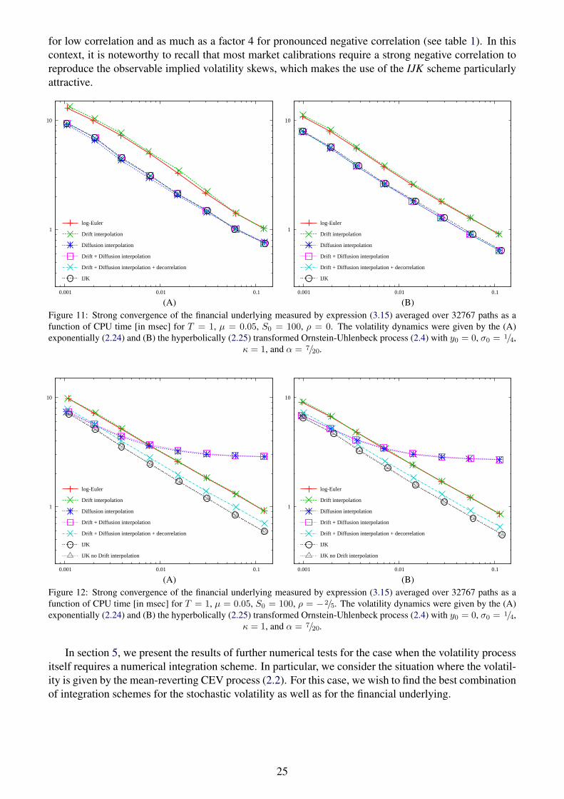
for low correlation and as much as a factor 4 for pronounced negative correlation (see table 1). In thiscontext, it is noteworthy to recall that most market calibrations require a strong negative correlation toreproduce the observable implied volatility skews, which makes the use of the IJK scheme particularlyattractive.

(A)

1

10

0.001 0.01 0.1

log-Euler

Drift interpolation




IJK

(B)

1

10

0.001 0.01 0.1

log-Euler

Drift interpolation




IJK

Figure 11: Strong convergence of the financial underlying measured by expression (3.15) averaged over 32767 paths as afunction of CPU time [in msec] for T = 1, µ = 0.05, S0 = 100, ρ = 0. The volatility dynamics were given by the (A)exponentially (2.24) and (B) the hyperbolically (2.25) transformed Ornstein-Uhlenbeck process (2.4) with y0 = 0, σ0 = 1/4,

κ = 1, and α = 7/20.

(A)

1

10

0.001 0.01 0.1

log-Euler

Drift interpolation




IJK


(B)

1

10

0.001 0.01 0.1

log-Euler

Drift interpolation




IJK


Figure 12: Strong convergence of the financial underlying measured by expression (3.15) averaged over 32767 paths as afunction of CPU time [in msec] for T = 1, µ = 0.05, S0 = 100, ρ = −2/5. The volatility dynamics were given by the (A)exponentially (2.24) and (B) the hyperbolically (2.25) transformed Ornstein-Uhlenbeck process (2.4) with y0 = 0, σ0 = 1/4,

κ = 1, and α = 7/20.

In section 5, we present the results of further numerical tests for the case when the volatility processitself requires a numerical integration scheme. In particular, we consider the situation where the volatil-ity is given by the mean-reverting CEV process (2.2). For this case, we wish to find the best combinationof integration schemes for the stochastic volatility as well as for the financial underlying.

25

(A)

1

10

0.001 0.01 0.1

log-Euler

Drift interpolation




IJK


(B)

1

10

0.001 0.01 0.1

log-Euler

Drift interpolation




IJK


Figure 13: Strong convergence of the financial underlying measured by expression (3.15) averaged over 32767 paths as afunction of CPU time [in msec] for T = 1, µ = 0.05, S0 = 100, ρ = −4/5. The volatility dynamics were given by the (A)exponentially (2.24) and (B) the hyperbolically (2.25) transformed Ornstein-Uhlenbeck process (2.4) with y0 = 0, σ0 = 1/4,

κ = 1, and α = 7/20.

5 Numerical results for mean-reverting CEV volatility processes

In this section we go one step further as we consider a two-dimensional stochastic volatility modelwhere the stochastic volatility process is given by the mean-reverting CEV process (2.2). We alreadyrecognized in section 3 that the numerical results for the integration of a mean-reverting CEV processare sensitive to the size of the diffusion exponent q ∈ [1/2, 1]. Hence we focus on the two extremechoices the Brennan-Schwartz (3.23) and the Cox-Ingersoll-Ross (3.37) equation. In the following weconsider four schemes for the integration of stochastic volatility or variance:

1. Euler — (3.1) ,

2. Milstein — (A.4) ,

3. BMM — (3.7) ,

4. Pathwise Adapted Linearisation — (3.32) for Brennan-Schwartz and (3.44) for CIR .

We combine these with suitable integration schemes for the whole system. Specifically, we consider

1. Euler-Maruyama — (4.3) ,

2. IJK — (4.47) .

The Euler scheme was already the benchmark in section 4 where we developed the IJK scheme. It is ofinterest to see if the IJK scheme can preserve its advantage even if we have to integrate the stochasticvolatility process numerically.

In the following we concentrate on two different test cases. The first one is based on the Brennan-Schwartz equation (3.23) for the modelling of the stochastic volatility. This equation is directly coupledto the underlying with exponent p = 1/2

dSt = µStdt+√VtStdWt ,

dVt = κ (θ − Vt) dt+ αVtdZt .(5.1)

26

The parameter configuration is chosen as follows St0 = 100, µ = 0.05, V0 = θ = 1/16, κ = 1, α = 0.5where we present results for different levels of correlation ρ ∈ {0.0,−0.4,−0.8}.

As a second benchmark we consider the Heston model

dSt = µStdt+√VtStdWt ,

dVt = κ (θ − Vt) dt+ α√VtdZt ,

(5.2)

where the parameters are given by St0 = 100, µ = 0.05, V0 = θ = 1/16, κ = 1, α = 0.5. Again we showresults for decreasing correlation ρ ∈ {0.0,−0.4,−0.8}.

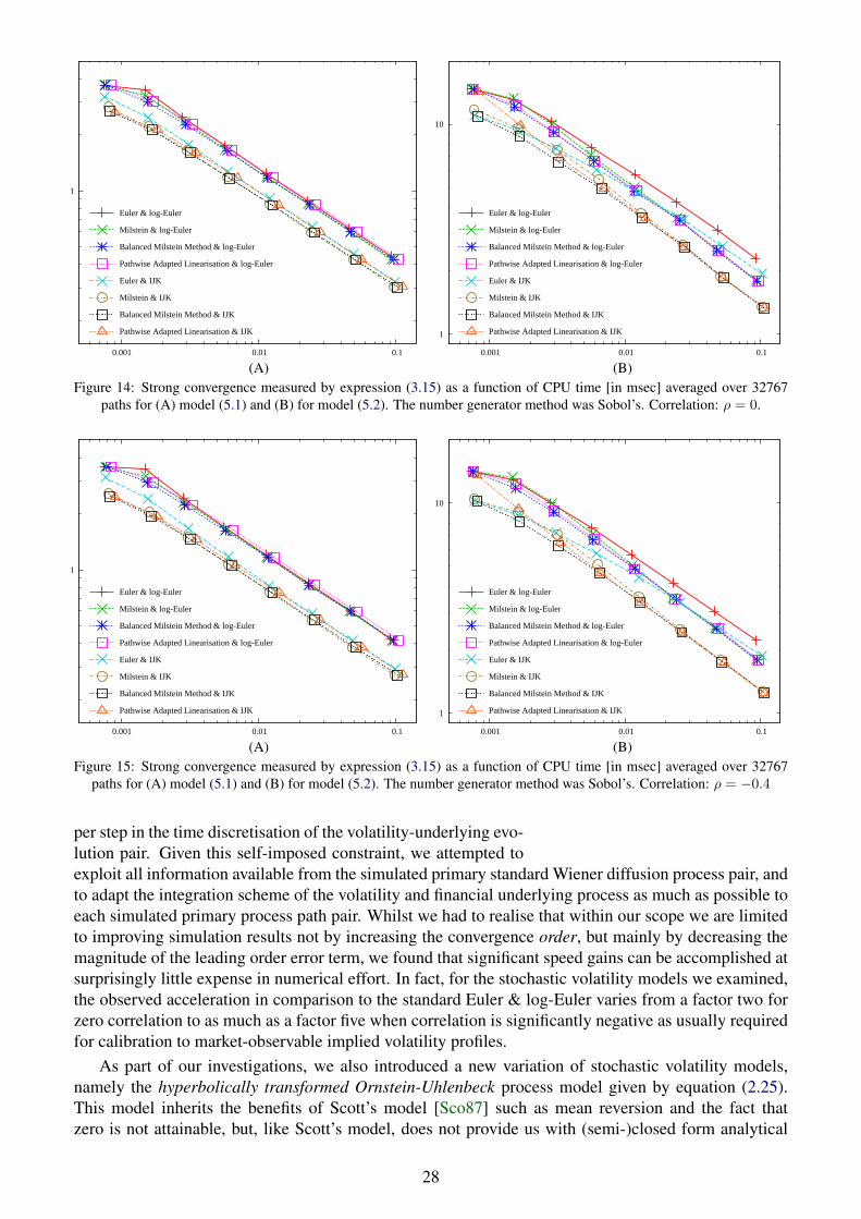
We see in figures 14–16 that the decisive point for the strong approximation quality is the choice ofthe integration scheme IJK as the integration of the stochastic volatility has just a minor impact on thenumerical results. In accordance with the numerical results of the last section, we can observe that theIJK scheme is at its most impressive when dealing with high correlation as in figure 16. In fact for highnegative correlation, the approximation efficiency of the IJK scheme in comparison to conventional Eu-ler & log-Euler methods appears to be even greater in the case when the volatility process itself requiresnumerical integration considering that the speed gain appears to be approximately a factor 5 in figure 16.

figure ρ (5.1) (5.2)14 0.0 2.1 2.615 -0.4 2.5 2.916 -0.8 4.6 4.5

Table 2: Average speed-up BMM &IJK (4.47) compared with Euler &

log-Euler (4.3).

Nonetheless, even if we can neglect the influence of the numeri-cal integration of the stochastic volatility process on the strong con-vergence behaviour of the underlying, the details of the integra-tion of the stochastic volatility process become important when pric-ing derivatives that are sensitive to the dynamics of the volatility.In that case, the results of section 3 can give guidance in the se-lection of the integration scheme for the mean-reverting CEV pro-cess. In any case, one should be aware of the fact that an un-

stable integration of the stochastic volatility can crash the integration of the whole system in thesense that the occurrence of spurious paths where variance crosses over to the negative domain canspoil the convergence behaviour irrecoverably as we saw in figure 5 (B) for the Milstein+ scheme.On that note, we have a closer look at figure 16 (B) where we see that the convergence behaviour of theMilstein-IJK scheme seems somewhat unexpected as the approximation error does not decrease whenhalving the stepsize from ∆t = 1 to ∆t = 1/2 even though this integration scheme is competitive tothe BMM-IJK scheme for small stepsizes. The explanation for this is surprisingly simple. In table 3we compare the percentage of non-positive paths for the integration of the stochastic volatility wherewe do not count those paths becoming non-positive in the final integration step5. With this countingconvention, no non-positive paths occur for ∆t = 1 as we only have to take a single step. In comparison,for ∆t = 1/2 we obtain the highest number of non-positive paths for the Milstein scheme which explainsthe bump in the convergence plot of Milstein-IJK in figure 16 (B). Thus, even in this very simple case ofestimating the strong convergence error of the financial underlying, an appropriate integration schemefor the stochastic volatility process is key to guaranteeing a stable approximation.

6 Conclusion

∆t Euler Milstein BMM

20 0 % 0 % 0 %2−1 23.9 % 33.2 % 0 %2−2 37.5 % 15.7 % 0 %2−3 43.8 % 0.1 % 0 %2−4 46.7 % 0 % 0 %

Table 3: Number of non-positive stochasticvolatility paths in figure 16 (B).

In this article, we discussed various Monte-Carlo approximationschemes for stochastic volatility diffusion models. Our main fo-cus was on the strong convergence behaviour as an indicator forthe valuation of path dependent derivatives. In order to main-tain the ability to apply exogenous variance reduction techniquessuch as low discrepancy numbers, importance sampling, and oth-ers [Jac02, Gla03], with ease, we restricted our research to meth-ods that effectively require only two simulated uniform variates

5It is of minor importance if one path becomes negative or zero in the last integration step as we do not have to use thefinal value as a starting point for the next integration step.

27

(A)

1

0.001 0.01 0.1

Euler & log-Euler

Milstein & log-Euler

Balanced Milstein Method & log-Euler

Pathwise Adapted Linearisation & log-Euler

Euler & IJK

Milstein & IJK

Balanced Milstein Method & IJK

Pathwise Adapted Linearisation & IJK

(B)

1

10

0.001 0.01 0.1

Euler & log-Euler




Euler & IJK

Milstein & IJK



Figure 14: Strong convergence measured by expression (3.15) as a function of CPU time [in msec] averaged over 32767paths for (A) model (5.1) and (B) for model (5.2). The number generator method was Sobol’s. Correlation: ρ = 0.

(A)

1

0.001 0.01 0.1

Euler & log-Euler




Euler & IJK

Milstein & IJK



(B)

1

10

0.001 0.01 0.1

Euler & log-Euler




Euler & IJK

Milstein & IJK



Figure 15: Strong convergence measured by expression (3.15) as a function of CPU time [in msec] averaged over 32767paths for (A) model (5.1) and (B) for model (5.2). The number generator method was Sobol’s. Correlation: ρ = −0.4

per step in the time discretisation of the volatility-underlying evo-lution pair. Given this self-imposed constraint, we attempted toexploit all information available from the simulated primary standard Wiener diffusion process pair, andto adapt the integration scheme of the volatility and financial underlying process as much as possible toeach simulated primary process path pair. Whilst we had to realise that within our scope we are limitedto improving simulation results not by increasing the convergence order, but mainly by decreasing themagnitude of the leading order error term, we found that significant speed gains can be accomplished atsurprisingly little expense in numerical effort. In fact, for the stochastic volatility models we examined,the observed acceleration in comparison to the standard Euler & log-Euler varies from a factor two forzero correlation to as much as a factor five when correlation is significantly negative as usually requiredfor calibration to market-observable implied volatility profiles.

As part of our investigations, we also introduced a new variation of stochastic volatility models,namely the hyperbolically transformed Ornstein-Uhlenbeck process model given by equation (2.25).This model inherits the benefits of Scott’s model [Sco87] such as mean reversion and the fact thatzero is not attainable, but, like Scott’s model, does not provide us with (semi-)closed form analytical

28

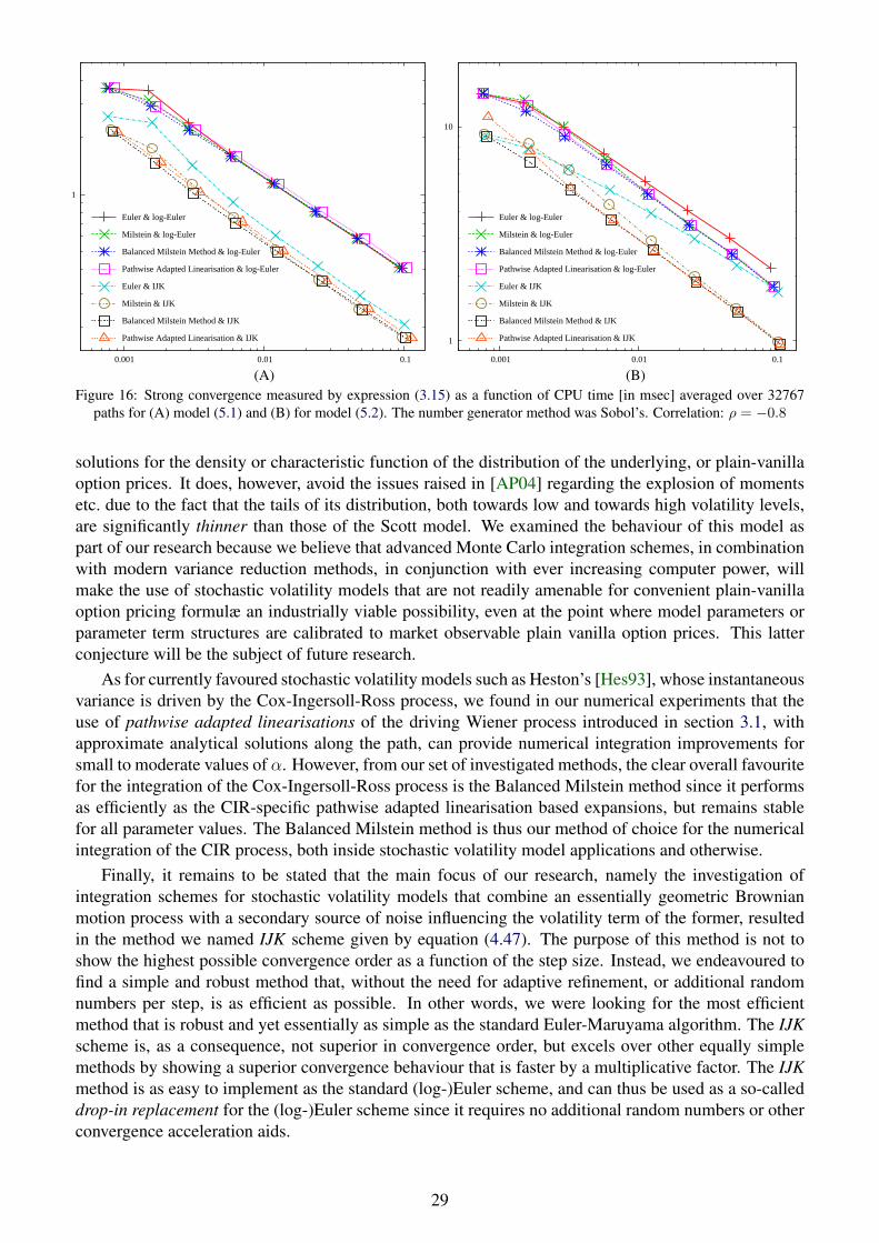
(A)

1

0.001 0.01 0.1

Euler & log-Euler




Euler & IJK

Milstein & IJK



(B)

1

10

0.001 0.01 0.1

Euler & log-Euler




Euler & IJK

Milstein & IJK



Figure 16: Strong convergence measured by expression (3.15) as a function of CPU time [in msec] averaged over 32767paths for (A) model (5.1) and (B) for model (5.2). The number generator method was Sobol’s. Correlation: ρ = −0.8

solutions for the density or characteristic function of the distribution of the underlying, or plain-vanillaoption prices. It does, however, avoid the issues raised in [AP04] regarding the explosion of momentsetc. due to the fact that the tails of its distribution, both towards low and towards high volatility levels,are significantly thinner than those of the Scott model. We examined the behaviour of this model aspart of our research because we believe that advanced Monte Carlo integration schemes, in combinationwith modern variance reduction methods, in conjunction with ever increasing computer power, willmake the use of stochastic volatility models that are not readily amenable for convenient plain-vanillaoption pricing formulæ an industrially viable possibility, even at the point where model parameters orparameter term structures are calibrated to market observable plain vanilla option prices. This latterconjecture will be the subject of future research.

As for currently favoured stochastic volatility models such as Heston’s [Hes93], whose instantaneousvariance is driven by the Cox-Ingersoll-Ross process, we found in our numerical experiments that theuse of pathwise adapted linearisations of the driving Wiener process introduced in section 3.1, withapproximate analytical solutions along the path, can provide numerical integration improvements forsmall to moderate values of α. However, from our set of investigated methods, the clear overall favouritefor the integration of the Cox-Ingersoll-Ross process is the Balanced Milstein method since it performsas efficiently as the CIR-specific pathwise adapted linearisation based expansions, but remains stablefor all parameter values. The Balanced Milstein method is thus our method of choice for the numericalintegration of the CIR process, both inside stochastic volatility model applications and otherwise.

Finally, it remains to be stated that the main focus of our research, namely the investigation ofintegration schemes for stochastic volatility models that combine an essentially geometric Brownianmotion process with a secondary source of noise influencing the volatility term of the former, resultedin the method we named IJK scheme given by equation (4.47). The purpose of this method is not toshow the highest possible convergence order as a function of the step size. Instead, we endeavoured tofind a simple and robust method that, without the need for adaptive refinement, or additional randomnumbers per step, is as efficient as possible. In other words, we were looking for the most efficientmethod that is robust and yet essentially as simple as the standard Euler-Maruyama algorithm. The IJKscheme is, as a consequence, not superior in convergence order, but excels over other equally simplemethods by showing a superior convergence behaviour that is faster by a multiplicative factor. The IJKmethod is as easy to implement as the standard (log-)Euler scheme, and can thus be used as a so-calleddrop-in replacement for the (log-)Euler scheme since it requires no additional random numbers or otherconvergence acceleration aids.

29

A Milstein schemes

A.1 The one-dimensional Milstein method

The Milstein scheme [Mil74] for the stochastic differential equation

dx = a(x)dt+ b(x)dW (A.1)

can be derived from the Ito-Taylor expansion [KP99, equation 5.5.4]

xt = x0 + a0

t∫0

ds+ b0

t∫0

dWs + b′0b0

t∫0

s∫0

dWu dWs

+ a′0b0

t∫0

s∫0

dWu ds+(a0b

′0 + 1

2b′′0b

20

) t∫0

s∫0

du dWs +(b0 b

′0

2+ b′′0b

20

) t∫0

s∫0

u∫0

dWr dWu dWs

(A.2)

+O(t2)

with a0 = a(x0), etc. Retaining terms up to order O(t), and evaluating the integral

I(1,1)(t) :=

t∫0

s∫0

dWu dWs = 12

(W 2

t − t), (A.3)

assuming (without loss of generality) that W0 = 0, we obtain the one-dimensional Milstein scheme

xtn+1 = xtn + a(xtn)∆tn + b(xtn)∆Wn + 12b′(xtn)b(xtn)

(∆W 2

n −∆tn). (A.4)

Applied to equation (2.2), we obtain

V Milsteintn+1

= Vtn + κ(θ − Vtn)∆tn + αV qtn∆Zn + 1

2α2qV 2q−1

tn

(∆Z2

n −∆tn). (A.5)

A.2 The Milstein+ scheme

All of the explicitly given integral terms on the second line of (A.2)

I(1,0)(t) =

t∫0

s∫0

dWu ds (A.6)

I(0,1)(t) =

t∫0

s∫0

du dWs = Wt · t− I(1,0)(t) (A.7)

I(1,1,1)(t) =

t∫0

s∫0

u∫0

dWr dWu dWs = 16W 3

t − 12Wt · t (A.8)

can be expressed in terms of the primary constituentsWt and I(1,0)(t). The two-dimensional distributionof the random numbers Wt and I(1,0)(t) is given by a bivariate Gaussian law with mean (0, 0) andcovariance matrix (

t t2/ 2t2/ 2 t3/ 3

). (A.9)

This means,I(1,0)(t) ∼ 1

2·Wt · t+ 1

2√

3· t3/2y (A.10)

30

with y ∼ N (0, 1), and thus the distribution of xt is given by

xt ∼ x0 + a0 · t+ b0 ·Wt + 12b′0b0

(W 2

t − t)

+ 16

(b0 b

′0

2+ b′′0b

20

)·W 3

t +(a0b

′0 − 1

2b0 b

′0

2)·Wt · t (A.11)

+(a′0b0 − a0b

′0 − 1

2b′′0b

20

)·[

12·Wt · t+ 1

2√

3· t3/2y

]+O(t2) .

Hence, in order to fully cater for all terms to order O(t3/2), an extra source of randomness is required.

It can also be seen that, conditional on a given value for Wt, the terms of order O(t3/2) have non-zero

expectation. This means, that, not accounting for the terms on the second and third line of (A.11), i.e.the terms not present in the standard Milstein scheme, introduces a conditional bias given by

16

[b0 b

′0

2+ b′′0b

20

]·W 3

t + 12

[a′0b0 + a0b

′0 − b0 b

′0

2 − 12b′′0b

20

]·Wt · t . (A.12)

This bias can be corrected by simply adding these terms to the Milstein scheme which gives us

xtn+1 = xtn + a(xtn)∆tn + b(xtn)∆Wn + 12b′(xtn)b(xtn)

(∆W 2

n −∆tn)

+ 16

[b(xtn) b′(xtn)

2+ b′′(xtn)b(xtn)2

]∆W 3

n (A.13)

+ 12

[a′(xtn)b(xtn) + a(xtn)b′(xtn)− b(xtn) b′(xtn)

2 − 12b′′(xtn)b(xtn)2

]∆Wn∆tn .

For the sake of brevity in the main text, we refer to this method as Milstein+. An alternative way toarrive at the approximation

I(1,0)(t) ; 12·Wt · t (A.14)

at the core of this scheme is to look for the most likely or the expected value of I(1,0)(t) conditional on thediscretised path forWt, i.e. in the filtration generated by the increments ∆Wn. Newton [New91, New94]introduced the idea of strong asymptotically efficient schemes following a similar line of reasoning andresulting in the approximation on (A.14). Specifically for the term I(1,0)(t), it so happens that the mostlikely and the expected value conditional on the discretised path {∆Wn} are both given by (A.14). Still,the advantage of the Milstein+ scheme over the original Milstein scheme is not that it has a higherconvergence order but that it reduces the magnitude coefficient of the leading order error terms.

Applied to equation (2.2), the Milstein+ scheme reads

V Milstein+tn+1

= Vtn + κ(θ − Vtn)∆tn + αV qtn∆Zn + 1

2α2qV 2q−1

tn

(∆Z2

n −∆tn)

+ 16α3q(2q − 1)V 3q−2

tn ∆Z3n

+ 12

[καθqV q−1

tn − κα(q + 1)V qtn −

12α3q (3q − 1)V 3q−2

tn

]∆Zn∆tn . (A.15)

A.3 The Milstein scheme for stochastic volatility systems

For the N -dimensional system of stochastic differential equations

dx = a(x)dt+B(x)dW , (A.16)

with a ∈ C1(RN ,RN) and B ∈ C2(RN ,RN×N),∀i = 1, . . . ,M and uncorrelated Brownian motionsW ∈ RN , the i-th component of the multidimensional Milstein scheme is

xi(t+ ∆t) = xi(t) + ai∆t+M∑

j=1

bij∆Wj +M∑

j,k,l=1

bjk(∂xjbil)I(k,l)︸︷︷︸

Milstein term

, (A.17)

31

wherein all of the coefficient functions ai(·) and bij(·), etc., are to be evaluated with x(t). We define thedouble Ito integral I(k,l) as

I(k,l) =

t+∆t∫s=t

s∫u=t

dWk(u) dWl(s) . (A.18)

For k = l, it simplifies toI(k,k) = 1

2

(∆W 2

k −∆t). (A.19)

For the stochastic volatility system (2.1) and (2.2), we use a Cholesky decomposition of the correlatedBrownian motions

dW = ρ′dW1 + ρ dW2 (A.20)dZ = dW2 (A.21)

with ρ′ :=√

1− ρ2 and set x1 := lnS and x2 := V to obtain from (2.1) and (2.2) the coupled stochasticdifferential equations(

dx1

dx2

)=

(µ− 1

2x2p

2

κ(θ − x2)

)dt +

(ρ′xp

2 ρ xp2

0 αxq2

)(dW1

dW2

). (A.22)

Since the volatility process x2 is not influenced directly by the dynamics for x1, the Milstein schemefor x2 is given by the standard one-dimensional formula (A.5). For x1, the fact that b21 = 0 and∂x1B(x) = 0 simplifies the calculation of the Milstein term:

M∑j,k,l=1

bjk(∂xjb1l)I(k,l) = b22(∂x2b11)I(2,1) + b22(∂x2b12)I(2,2)

= αpxp+q−12

(ρ′I(2,1) + ρI(2,2)

). (A.23)

References

[AA00] L. Andersen and J. Andreasen. Volatility Skews and Extensions of the Libor Market Model.Applied Mathematical Finance, 7(1):1–32, March 2000.

[Abe04] K.E.S. Abe. Strong Taylor Schemes for Stochastic Volatility. Working paper, 2004. www.maths.ox.ac.uk/∼schmitz/project2.htm.

[ABR01] L. Andersen and R. Brotherton-Ratcliffe. Extended Libor Market Models with StochasticVolatility. Working paper, Gen Re Securities, 2001.

[AP04] L. Andersen and V. Piterbarg. Moment Explosions in Stochastic Volatilty Models. Technicalreport, Bank of America, 2004. ssrn.com/abstract=559481.

[Bec80] S. Beckers. The constant elasticity of variance model and its implications for option pricing.Journal of Finance, XXXV(3):661–673, June 1980.

[BK04] M. Broadie and O. Kaya. Exact Simulation of Stochastic Volatility and other Affine JumpDiffusion Processes. Working paper, Columbia University, New York, 2004. www.orie.cornell.edu/∼aberndt/FEseminar/papers04/exact sim 200409.pdf.

[BS73] F. Black and M. Scholes. The Pricing of Options and Corporate Liabilities. Journal ofPolitical Economy, pages 637–654, 1973.

32

www.maths.ox.ac.uk/~schmitz/project2.htm

www.maths.ox.ac.uk/~schmitz/project2.htm

ssrn.com/abstract=559481

www.orie.cornell.edu/~aberndt/FEseminar/papers04/exact_sim_200409.pdf

www.orie.cornell.edu/~aberndt/FEseminar/papers04/exact_sim_200409.pdf

[BS80] M.J. Brennan and E.S. Schwartz. Analyzing convertible bonds. Journal of Financial andQuantitative Analysis, 15:907–929, 1980.

[CIR85] J. C. Cox, J. E. Ingersoll, and S. A. Ross. A theory of the term structure of interest rates.Econometrica, 53:385–408, 1985.

[CKLS92] C.K. Chan, G.A. Karolyi, F.A. Longstaff, and A.B. Sanders. An empirical comparison ofalternate models of the short-term interest rate. Journal of Finance, pages 1209–1227, 1992.www.cob.ohio-state.edu/∼sanders/ckls.pdf.

[Cox75] J. C. Cox. Notes on option pricing I: Constant elasticity of variance diffusions. Workingpaper, Stanford University, 1975.

[CR76] J. C. Cox and S. A. Ross. The valuation of options for alternative stochastic processes.Journal of Financial Economics, 3:145–166, March 1976.

[Doo42] J. L. Doob. The Brownian Movement and Stochastic Equations. The Annals of Mathematics,43:351–369, April 1942.

[Dos77] H. Doss. Liens entre equations differentielles stochastiques ordinaires. Annales de l’InstitutHenrie Poincare. Probabilites et Statistiques, 13:99–125, 1977.

[Eul68] L. Euler. Institutiones Calculi Integralis. 1768.

[GL94] J.G. Gaines and T.J. Lyons. Random Generation of Stochastic Area Integrals. SIAM Journalon Applied Mathematics, 54(4):1132–1146, 1994.

[Gla03] P. Glasserman. Monte Carlo Methods in Financial Engineering. Springer, 2003.

[GY93] H. Geman and M. Yor. Bessel Processes, Asian Options, and Perpetuities. MathematicalFinance, 3:349–375, 1993.

[Hes93] S. L. Heston. A closed-form solution for options with stochastic volatility with applicationsto bond and currency options. The Review of Financial Studies, 6:327–343, 1993.

[HW88] J. Hull and A. White. An Analysis of the Bias in Option Pricing Caused by a StochasticVolatility. Advances in Futures and Options Research, 3:27–61, 1988.

[HW93] M. Hogan and K. Weintraub. The Lognormal Interest Rate Model and Eurodollar Futures.Discussion paper, Citibank, New York, 1993.

[Jac02] P. Jackel. Monte Carlo methods in finance. John Wiley and Sons, February 2002.

[Kah04] C. Kahl. Positive numerical integration of stochastic differential equations. Master’s thesis,Bergische Universitat Wuppertal, 2004. www.math.uni-wuppertal.de/∼kahl/publications/DT.pdf.

[KJ05] C. Kahl and P. Jackel. Not-so-complex logarithms in the Heston model. Wilmott, September,September 2005.

[KP99] P. E. Kloeden and E. Platen. Numerical Solution of Stochastic Differential Equations.Springer, 1992, 1995, 1999.

[KS91] I. Karatzas and S. E. Shreve. Brownian motion and Stochastic Calculus. Springer, 1991.

[KS05] C. Kahl and H. Schurz. Balanced Milstein Methods for Ordinary SDEs. Technical report,Department of Mathematics, Southern Illinois University, 2005.

33

www.cob.ohio-state.edu/~sanders/ckls.pdf

www.math.uni-wuppertal.de/~kahl/publications/DT.pdf

www.math.uni-wuppertal.de/~kahl/publications/DT.pdf

[KT81] S. Karlin and M. Taylor. A Second Course in Stochastic Processes. Academic Press, 1981.

[Lev51] P. Levy. Wiener’s random function, and other Laplacian random functions. In Proceedingsof the Second Berkeley Symposium on Mathematical Statistics and Probability, 1950, pages171–187, Berkeley and Los Angeles, 1951. University of California Press.

[MAP76] G. Marsaglia, K. Anantharayanan, and N.J. Paul. Improvements on fast methods for gener-ating normal random variables. Information Processing Letters, 5:27–30, 1976.

[Mar55] G. Maruyama. Continuous Markov processes and stochastic equations. Rendiconti delCircolo Matematico di Palermo, 4:48–90, 1955.

[Mil74] G. N. Milshtein. Approximate integration of stochastic differential equations. Theory ofProbability and Applications, 19:557–562, 1974.

[MMB64] G. Marsaglia, M.D. MacLaren, and T.A. Bray. A fast procedure for generating normalrandom variables. Communications of the ACM, 5:27–30, 1964.

[MN98] M. Matsumoto and T. Nishimura. Mersenne Twister: A 623-dimensionally equidistributeduniform pseudorandom number generator. ACM Trans. on Modeling and Computer Simu-lation, 8(1):3–30, January 1998.

[MPS98] G. N. Milshtein, E. Platen, and H. Schurz. Balanced implicit methods for stiff stochasticsystems. SIAM, 38(3):1010–1019, 1998.

[New91] N. J. Newton. Asymptotically efficient Runge-Kutta methods for a class of Ito andStratonovich equations. SIAM Journal of Applied Mathematics, 51:542–567, 1991.

[New94] N. J. Newton. Variance reduction for simulated diffusions. Siam Journal of Applied Mathe-matics, 54:1780–1805, 1994.

[PT85] E. Pardoux and M. Talay. Discretization and simulation of stochastic differential equations.Acta Applicandae Mathematica, 3:23–47, 1985.

[Sch96] H. Schurz. Numerical Regularization for SDE’s: Construction of nonnegative solutions.Dynamical Systems and Applications, 5:323–352, 1996.

[Sco87] L. Scott. Option Pricing When the Variance Changes Randomly: Theory, Estimation andAn Application. Journal of Financial and Quantitative Analysis, 22:419–438, December1987.

[SS91] E. M. Stein and J. C. Stein. Stock Price Distribution with Stochastic Volatility : An AnalyticApproach. Review of Financial Studies, 4:727–752, 1991.

[SS94] K. Sandmann and D. Sondermann. On the stability of log-normal interest rate models andthe pricing of Eurodollar futures. Discussion paper, Dept. of Statistics, Faculty of Eco-nomics, SFB 303, Universitat Bonn, June 1994. ftp://ftp.wipol.uni-bonn.de/pub/RePEc/bon/bonsfb/bonsfb263.pdf.

[SS97a] K. Sandmann and D. Sondermann. A Note on the Stability of Lognormal Interest RateModels and the Pricing of Eurodollar Futures. Mathematical Finance, 7(2):119, April 1997.

[SS97b] K. Sandmann and D. Sondermann. Log-Normal Interest Rate Models: Stability and Method-ology. Discussion paper, Dept. of Statistics, Faculty of Economics, SFB 303, Univer-sitat Bonn, January 1997. ftp://ftp.wipol.uni-bonn.de/pub/RePEc/bon/bonsfb/bonsfb398.pdf.

34

ftp://ftp.wipol.uni-bonn.de/pub/RePEc/bon/bonsfb/bonsfb263.pdf




[SZ99] R. Schobel and J. Zhu. Stochastic Volatility With an Ornstein Uhlenbeck Process: AnExtension. European Finance Review, 3:23–46, 1999. ssrn.com/abstract=100831.

[UO30] G.E. Uhlenbeck and L.S. Ornstein. On the theory of Brownian motion. Physics Review,36:823–841, 1930.

[Wig87] J. Wiggins. Option values under stochastic volatility: Theory and empirical estimates. Jour-nal of Financial Economics, 19:351–372, 1987.

[WZ65] E. Wong and M. Zakai. On the convergence of ordinary integrals to stochastic integrals.Ann. Math. Stat., 36:1560–1564, 1965.

35

ssrn.com/abstract=100831

fast strong approximation monte-carlo schemes for ...kahl/publications/faststrong... · fast strong...

Documents