fast user’s guide technical report - nwtc information portal
TRANSCRIPT

National Renewable Energy Laboratory1617 Cole Boulevard, Golden, Colorado 80401-3393 303-275-3000 • www.nrel.gov
Operated for the U.S. Department of Energy Office of Energy Efficiency and Renewable Energy by Midwest Research Institute • Battelle
Contract No. DE-AC36-99-GO10337
National Renewable Energy Laboratory Innovation for Our Energy Future
A national laboratory of the U.S. Department of EnergyOffice of Energy Efficiency & Renewable Energy
NREL is operated by Midwest Research Institute Battelle Contract No. DE-AC36-99-GO10337
Technical Report NREL/EL-500-38230 August 2005
FAST User’s Guide Jason M. Jonkman, Marshall L. Buhl Jr.


National Renewable Energy Laboratory1617 Cole Boulevard, Golden, Colorado 80401-3393 303-275-3000 • www.nrel.gov
Operated for the U.S. Department of Energy Office of Energy Efficiency and Renewable Energy by Midwest Research Institute • Battelle
Contract No. DE-AC36-99-GO10337
Technical Report
NREL/EL-500-38230 August 2005
FAST User’s Guide Jason M. Jonkman, Marshall L. Buhl Jr.

NOTICE
This report was prepared as an account of work sponsored by an agency of the United States government. Neither the United States government nor any agency thereof, nor any of their employees, makes any warranty, express or implied, or assumes any legal liability or responsibility for the accuracy, completeness, or usefulness of any information, apparatus, product, or process disclosed, or represents that its use would not infringe privately owned rights. Reference herein to any specific commercial product, process, or service by trade name, trademark, manufacturer, or otherwise does not necessarily constitute or imply its endorsement, recommendation, or favoring by the United States government or any agency thereof. The views and opinions of authors expressed herein do not necessarily state or reflect those of the United States government or any agency thereof.
Available electronically at http://www.osti.gov/bridge
Available for a processing fee to U.S. Department of Energy and its contractors, in paper, from:
U.S. Department of Energy Office of Scientific and Technical Information P.O. Box 62 Oak Ridge, TN 37831-0062 phone: 865.576.8401 fax: 865.576.5728 email: mailto:[email protected]
Available for sale to the public, in paper, from: U.S. Department of Commerce National Technical Information Service 5285 Port Royal Road Springfield, VA 22161 phone: 800.553.6847 fax: 703.605.6900 email: [email protected] online ordering: http://www.ntis.gov/ordering.htm
Printed on paper containing at least 50% wastepaper, including 20% postconsumer waste
i
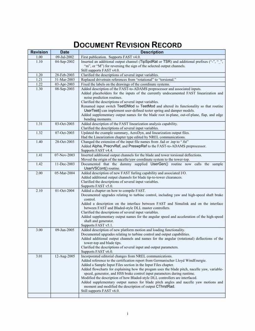
DOCUMENT REVISION RECORD Revision Date Description
1.00 09-Jul-2002 First publication. Supports FAST v4.0. 1.10 04-Sep-2002 Inserted an additional output channel (TipSpdRat or TSR) and additional prefixes (“-”, “_”,
“m”, or “M”) for reversing the sign of the selected output channels. Still supports FAST v4.0.
1.20 28-Feb-2003 Clarified the descriptions of several input variables. 1.21 31-Mar-2003 Replaced drivetrain references from “rotational” to “torsional.” 1.22 03-Apr-2003 Fixed the labels on the drawings of the coordinate systems. 1.30 08-Sep-2003 Added description of the FAST-to-ADAMS preprocessor and associated inputs.
Added placeholders for the inputs of the currently undocumented FAST linearization and noise prediction routines.
Clarified the descriptions of several input variables. Renamed input switch TeetDMod to TeetMod and altered its functionality so that routine
UserTeet() can implement user-defined teeter spring and damper models. Added supplementary output names for the blade root in-plane, out-of-plane, flap, and edge
bending moments. 1.31 03-Oct-2003 Added description of the FAST linearization analysis capability.
Clarified the descriptions of several input variables. 1.32 07-Oct-2003 Updated the example summary, AeroDyn, and linearization output files.
Had the Linearization chapter type edited by NREL communications. 1.40 28-Oct-2003 Changed the extension of the input file names from .fad or .inp to “.fst”
Added Alpha, PrecrvRef, and PreswpRef to the FAST-to-ADAMS preprocessor. Supports FAST v4.4.
1.41 07-Nov-2003 Inserted additional output channels for the blade and tower torsional deflections. Moved the origin of the nacelle/yaw coordinate system to the tower-top.
1.42 11-Dec-2003 Documented that the dummy supplied UserGen() routine now calls the sample UserVSCont() routine.
2.00 05-Mar-2004 Added description of new FAST furling capability and associated I/O. Added additional output channels for blade tip-to-tower clearances. Clarified the descriptions of several input variables. Supports FAST v5.0.
2.10 01-Oct-2004 Added a chapter on how to compile FAST. Documented upgrades relating to turbine control, including yaw and high-speed shaft brake
control. Added a description on the interface between FAST and Simulink and on the interface
between FAST and Bladed-style DLL master controllers. Clarified the descriptions of several input variables. Added supplementary output names for the angular speed and acceleration of the high-speed
shaft and generator. Supports FAST v5.1.
3.00 09-Jun-2005 Added description of new platform motion and loading functionality. Documented upgrades relating to turbine control and output capabilities. Added additional output channels and names for the angular (rotational) deflections of the
tower-top and blade tips. Clarified the descriptions of several input and output parameters. Supports FAST v6.0.
3.01 12-Aug-2005 Incorporated editorial changes from NREL communications. Added reference to the certification report from Germanischer Lloyd WindEnergie. Added a Sample Input Files section in the Input Files chapter. Added flowcharts for explaining how the progam uses the blade pitch, nacelle yaw, variable-
speed, generator, and HSS brake control input parameters during runtime. Modified the description of how Bladed-style DLL controllers are interfaced. Added supplementary output names for blade pitch angles and nacelle yaw motions and
moment and modified the description of output CThrstRad. Still supports FAST v6.0.

FAST User's Guide iii Last updated on August 12, 2005 for version 6.0
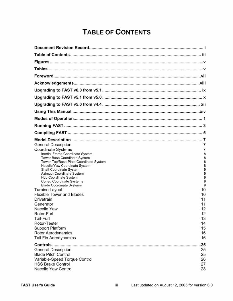
TABLE OF CONTENTS
Document Revision Record................................................................................................ i Table of Contents.............................................................................................................. iii Figures.................................................................................................................................v Tables...................................................................................................................................v Foreword............................................................................................................................vii Acknowledgements..........................................................................................................viii Upgrading to FAST v6.0 from v5.1 ................................................................................... ix Upgrading to FAST v5.1 from v5.0 .................................................................................... x Upgrading to FAST v5.0 from v4.4 .................................................................................. xii Using This Manual............................................................................................................xiv Modes of Operation............................................................................................................ 1 Running FAST .................................................................................................................... 3 Compiling FAST ................................................................................................................. 5 Model Description .............................................................................................................. 7 General Description 7 Coordinate Systems 7
Inertial Frame Coordinate System 8 Tower-Base Coordinate System 8 Tower-Top/Base-Plate Coordinate System 8 Nacelle/Yaw Coordinate System 8 Shaft Coordinate System 9 Azimuth Coordinate System 9 Hub Coordinate System 9 Coned Coordinate Systems 9 Blade Coordinate Systems 9
Turbine Layout 10 Flexible Tower and Blades 10 Drivetrain 11 Generator 11 Nacelle Yaw 12 Rotor-Furl 12 Tail-Furl 13 Rotor-Teeter 14 Support Platform 15 Rotor Aerodynamics 16 Tail Fin Aerodynamics 16 Controls .............................................................................................................................25 General Description 25 Blade Pitch Control 25 Variable-Speed Torque Control 26 HSS Brake Control 27 Nacelle Yaw Control 28
FAST User's Guide iv Last updated on August 12, 2005 for version 6.0
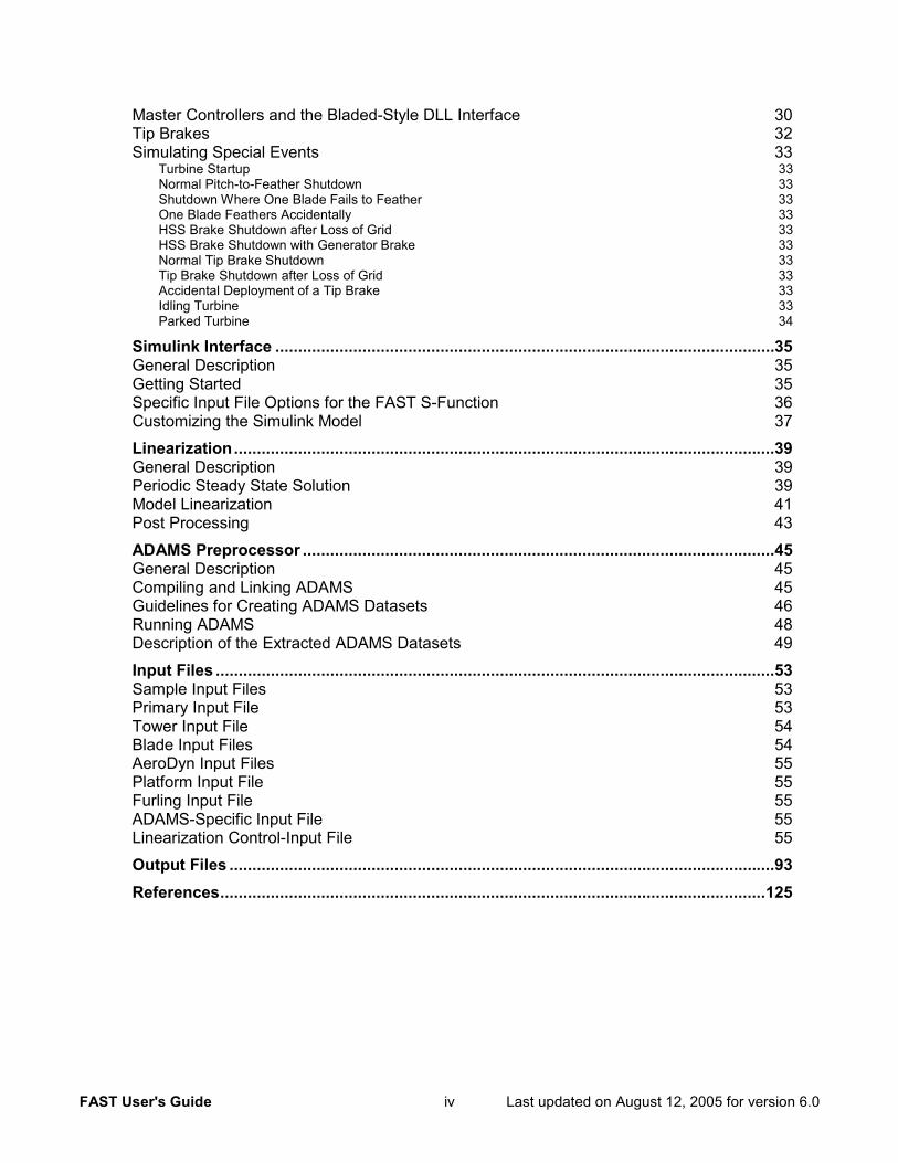
Master Controllers and the Bladed-Style DLL Interface 30 Tip Brakes 32 Simulating Special Events 33
Turbine Startup 33 Normal Pitch-to-Feather Shutdown 33 Shutdown Where One Blade Fails to Feather 33 One Blade Feathers Accidentally 33 HSS Brake Shutdown after Loss of Grid 33 HSS Brake Shutdown with Generator Brake 33 Normal Tip Brake Shutdown 33 Tip Brake Shutdown after Loss of Grid 33 Accidental Deployment of a Tip Brake 33 Idling Turbine 33 Parked Turbine 34
Simulink Interface .............................................................................................................35 General Description 35 Getting Started 35 Specific Input File Options for the FAST S-Function 36 Customizing the Simulink Model 37 Linearization......................................................................................................................39 General Description 39 Periodic Steady State Solution 39 Model Linearization 41 Post Processing 43 ADAMS Preprocessor .......................................................................................................45 General Description 45 Compiling and Linking ADAMS 45 Guidelines for Creating ADAMS Datasets 46 Running ADAMS 48 Description of the Extracted ADAMS Datasets 49 Input Files ..........................................................................................................................53 Sample Input Files 53 Primary Input File 53 Tower Input File 54 Blade Input Files 54 AeroDyn Input Files 55 Platform Input File 55 Furling Input File 55 ADAMS-Specific Input File 55 Linearization Control-Input File 55 Output Files .......................................................................................................................93 References.......................................................................................................................125
FAST User's Guide v Last updated on August 12, 2005 for version 6.0
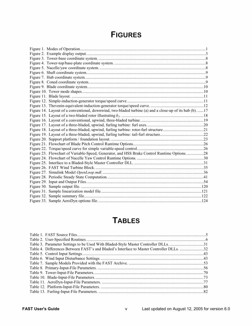
FIGURES
Figure 1. Modes of Operation.........................................................................................................................1 Figure 2. Example display output. ..................................................................................................................3 Figure 3. Tower-base coordinate system. .......................................................................................................8 Figure 4. Tower-top/base-plate coordinate system. ........................................................................................8 Figure 5. Nacelle/yaw coordinate system. ......................................................................................................8 Figure 6. Shaft coordinate system...................................................................................................................9 Figure 7. Hub coordinate system. ...................................................................................................................9 Figure 8. Coned coordinate system.................................................................................................................9 Figure 9. Blade coordinate system................................................................................................................10 Figure 10. Tower mode shapes. ....................................................................................................................10 Figure 11. Blade layout. ...............................................................................................................................11 Figure 12. Simple-induction-generator torque/speed curve..........................................................................11 Figure 13. Thevenin-equivalent-induction-generator torque/speed curve. ...................................................12 Figure 14. Layout of a conventional, downwind, two-bladed turbine (a) and a close-up of its hub (b). ......17 Figure 15. Layout of a two-bladed rotor illustrating δ3. ...............................................................................18 Figure 16. Layout of a conventional, upwind, three-bladed turbine. ............................................................19 Figure 17. Layout of a three-bladed, upwind, furling turbine: furl axes.......................................................20 Figure 18. Layout of a three-bladed, upwind, furling turbine: rotor-furl structure .......................................21 Figure 19. Layout of a three-bladed, upwind, furling turbine: tail-furl structure..........................................22 Figure 20. Support platform / foundation layout. .........................................................................................23 Figure 21. Flowchart of Blade Pitch Control Runtime Options....................................................................26 Figure 22. Torque/speed curve for simple variable-speed control................................................................26 Figure 23. Flowchart of Variable-Speed, Generator, and HSS Brake Control Runtime Options. ................28 Figure 24. Flowchart of Nacelle Yaw Control Runtime Options. ................................................................30 Figure 25. Interface to a Bladed-Style Master Controller DLL. ...................................................................31 Figure 26. FAST Wind Turbine Block. ........................................................................................................35 Figure 27. Simulink Model OpenLoop.mdl. .................................................................................................36 Figure 28. Periodic Steady State Computation. ............................................................................................41 Figure 29. Input and Output Files. ................................................................................................................54 Figure 30. Sample output file. ....................................................................................................................120 Figure 31. Sample linearization model file.................................................................................................121 Figure 32. Sample summary file.................................................................................................................122 Figure 33. Sample AeroDyn options file. ...................................................................................................124
TABLES
Table 1. FAST Source Files............................................................................................................................5 Table 2. User-Specified Routines. ..................................................................................................................6 Table 3. Parameter Settings to be Used With Bladed-Style Master Controller DLLs. .................................31 Table 4. Differences Between FAST’s and Bladed’s Interface to Master Controller DLLs. .......................32 Table 5. Control Input Settings.....................................................................................................................43 Table 6. Wind Input Disturbance Settings. ...................................................................................................43 Table 7. Sample Models Provided with the FAST Archive. ........................................................................53 Table 8. Primary-Input-File Parameters. ......................................................................................................56 Table 9. Tower-Input-File Parameters. .........................................................................................................70 Table 10. Blade-Input-File Parameters. ........................................................................................................73 Table 11. AeroDyn-Input-File Parameters. ..................................................................................................77 Table 12. Platform-Input-File Parameters. ...................................................................................................80 Table 13. Furling-Input-File Parameters. .....................................................................................................82
FAST User's Guide vi Last updated on August 12, 2005 for version 6.0
Table 14. ADAMS-Specific-Input-File Parameters......................................................................................88 Table 15. Linearization Control-Input-File Parameters. ...............................................................................90 Table 16. Output Parameters for Wind Motions...........................................................................................94 Table 17. Output Parameters for Blade 1 Tip Motions.................................................................................95 Table 18. Output Parameters for Blade 2 Tip Motions.................................................................................96 Table 19. Output Parameters for Blade 3 Tip Motions.................................................................................98 Table 20. Output Parameters for Blade 1 Local Span Motions. .................................................................100 Table 21. Output Parameters for Blade Pitch Motions. ..............................................................................101 Table 22. Output Parameters for Teeter Motions. ......................................................................................101 Table 23. Output Parameters for Shaft Motions. ........................................................................................102 Table 24. Output Parameters for Nacelle Inertial Measurement Unit Motions. .........................................103 Table 25. Output Parameters for Rotor-Furl Motions.................................................................................104 Table 26. Output Parameters for Tail-Furl Motions. ..................................................................................104 Table 27. Output Parameters for Nacelle Yaw Motions. ............................................................................104 Table 28. Output Parameters for Tower-Top, Yaw-Bearing Motions. .......................................................105 Table 29. Output Parameters for Local Tower Motions. ............................................................................107 Table 30. Output Parameters for Platform Motions....................................................................................108 Table 31. Output Parameters for Blade 1 Root Loads. ...............................................................................110 Table 32. Output Parameters for Blade 2 Root Loads. ...............................................................................111 Table 33. Output Parameters for Blade 3 Root Loads. ...............................................................................112 Table 34. Output Parameters for Blade 1 Local Span Loads......................................................................113 Table 35. Output Parameters for Hub and Rotor Loads. ............................................................................114 Table 36. Output Parameters for Shaft Strain-Gage Loads. .......................................................................115 Table 37. Output Parameters for Generator and HSS Loads. .....................................................................115 Table 38. Output Parameters for Rotor-Furl Bearing Loads. .....................................................................116 Table 39. Output Parameters for Tail-Furl Bearing Loads. ........................................................................116 Table 40. Output Parameters for Tail Fin Aerodynamic Loads..................................................................116 Table 41. Output Parameters for Tower-Top, Yaw-Bearing Loads............................................................117 Table 42. Output Parameters for Tower Base Loads. .................................................................................117 Table 43. Output Parameters for Local Tower Loads.................................................................................118 Table 44. Output Parameters for Platform Loads. ......................................................................................119
FAST User's Guide vii Last updated on August 12, 2005 for version 6.0
FOREWORD
The FAST (Fatigue, Aerodynamics, Structures, and Turbulence) Code is a comprehensive aeroelastic simulator capable of predicting both the extreme and fatigue loads of two- and three-bladed horizontal-axis wind turbines (HAWTs). This document covers the features of FAST and outlines its operating procedures.
The FAST Code is the result of the marriage of three distinct codes; the FAST2 Code for two-bladed HAWTs; the FAST3 Code for three-bladed HAWTs; and the AeroDyn (1) aerodynamics subroutines for HAWTs. While combining these three codes, changes were made in the computational loops and in the kinematic calculations of the FAST codes. An intermediate version of FAST, called FAST_AD, used different executable files for two- and three-bladed turbines. The version of FAST documented in this report, which was developed in 2002, uses a single executable for both types of turbines. These changes resulted in a code that runs very quickly, so the code is indeed, fast.
In 2003, additional features were added to the FAST Code, including the ability to develop periodic linearized state matrices for controls design and the ability to use FAST as a preprocessor for generating ADAMS® datasets of wind turbine models (“ADAMS” is used to imply “ADAMS®” throughout this document). Aeroacoustic noise prediction algorithms have also been introduced.
Additional features were added to the FAST Code again in 2004. New model features added include a lateral offset and skew angle of the rotor shaft, rotor-furling, tail-furling, tail inertia and aerodynamics, yaw control, and high-speed shaft (HSS) brake control. An interface has been developed between FAST and a master controller implemented as a dynamic-link-library (DLL) in the style of Garrad Hassan's Bladed wind turbine software package (2). An interface has also been developed between FAST and Simulink® with MATLAB® (“Simulink” and “MATLAB” are used to imply “Simulink®” and “MATLAB®” throughout this document), enabling users to implement advanced turbine controls in Simulink’s convenient block diagram form.
In 2005, FAST and ADAMS with AeroDyn were evaluated by Germanischer Lloyd WindEnergie and found suitable for "the calculation of onshore wind
turbine loads for design and certification" (3). Additional features were also added to the Codes. These include new nacelle inertial measurement unit and tower strain gage outputs, upgrades to the simple variable-speed control model, and new support platform motion and loading functionality. Despite the addition of six new platform motion degrees of freedom, the Code was also better-optimized so that it runs 15% faster than previous versions (or faster, depending on the options being modeled).
This manual is an updated subset of one originally written at Oregon State University (OSU) (4). The original manual included a detailed discussion of the theory behind FAST_AD (an earlier incarnation of FAST) and a validation of the code. For these two topics, please refer to the original. Also available is Buhl and others (5), which is a structural verification of FAST_AD against ADAMS. Both FAST and ADAMS use the AeroDyn subroutine set, so the structural-verification study did not provide any verification of the aerodynamics of FAST_AD. A more recent verification of FAST against ADAMS is provided in Jonkman and Buhl (6).
The Modes of Operation chapter describes the different types of analysis available in FAST and a brief description on how to run the code is provided in the Running FAST chapter. If you want to recompile FAST, you can find the information you’ll need in the Compiling FAST chapter. The Model Description chapter discusses the degrees of freedom for both two- and three-bladed HAWTs. The Controls chapter documents methods for actively controlling many aspects of the turbine operation during simulation. Active controls can also be implemented in Simulink as described in the Simulink Interface chapter. The Linearization chapter documents how to extract linearized wind turbine models out of FAST. The functionality of using FAST as a preprocessor for creating ADAMS datasets is documented in the ADAMS Preprocessor chapter. The Input Files chapter describes the various program input files. Finally, the Output Files chapter lists the possible output parameters. It also describes the optional summary and element output files.
FAST User's Guide viii Last updated on August 12, 2005 for version 6.0
ACKNOWLEDGEMENTS Funding for FAST development came from the
U.S. Department of Energy under contract No. DE-AC36-83CH10093 to the National Renewable Energy Laboratory (NREL). Later improvements were funded by the U.S. Department of Energy under contract No. DE-AC36-98-GO10337 to NREL.
The authors would like to thank Tim Weber, Lisa Freeman, and Ross Harman of OSU; Norm Weaver of InterWeaver Consulting; and Kirk Pierce, formerly of NREL, for their past developments of FAST and FAST_AD. We would also like to thank the folks at Windward Engineering for developing and interfacing
the AeroDyn routines that we link with the FAST structural-dynamics routines and for writing an example pitch-control routine. Tim McCoy of Global Energy Concepts and Craig Hansen of Windward Engineering took time from their busy schedules to review drafts of this manual. Our editors, Kathy O’Dell, Ruth Baranowski, and Janie Homan, helped a lot by converting our twisted prose into readable English. Another tip of the hat goes to the many folks in the wind-energy industry who tested FAST and provided us with their valuable feedback.
FAST User's Guide ix Last updated on August 12, 2005 for version 6.0
UPGRADING TO FAST V6.0 FROM V5.1 This section describes how to update input files
created previously for FAST v5.1 so that they are compatible with FAST v6.0. New users can skip to the section entitled Using This Manual.
FAST v6.0 contains an improvement to the simple variable-speed control model, a few upgrades and modifications to the output capabilities, and new support platform motion and loading functionality.
The simple variable-speed control model has been upgraded to include a linear transition Region 2½, in addition to the previously-available Regions 2 and 3. See the updated Variable-Speed Torque Control section of the Controls chapter and the Turbine Control section of Table 8 for more information.
You can now specify up to 5 strain gage locations along the tower for examining local tower motions and loads output, similar to what is available for blade 1. You can also specify the location in the nacelle of an inertial measurement unit (IMU)—this location is used for new nacelle motion outputs. See the Output section of Table 8 and the Output Files chapter for more information.
The new support platform motion and loading functionality represents a major expansion in the number of degrees of freedom and loading options available in FAST. Detailed information on these new features and associated inputs are presented throughout this manual where appropriate. In particular, see the Support Platform section and Figure 20 of the Model Description chapter, the Platform Input File section of the Input Files chapter, the Platform Model section of Table 8, and Table 12.
Despite the addition of six new platform motion DOFs (translational surge, sway, and heave and rotational roll, pitch and yaw), the Code was also better-optimized so that it runs 15% faster than previous versions (or faster, depending on the options being modeled).
With the addition of support platform motion functionality, it made sense to add more information to the FAST summary (.fsm) file. See the Output Files chapter, especially Figure 32, for more information
It also made made sense to rename some of the output parameters. The output channels WindVxt, WindVyt, and WindVzt in FAST v5.1 were renamed to WindVxi, WindVyi, and WindVzi in v6.0, respectively, since the wind speeds relative to the inertia frame (i) are now more important than the wind speeds relative to the tower-base frame (t), which can now move relative to the inertia frame. WindVxi, WindVyi, and WindVzi in FAST v6.0 will give the same results as WindVxt, WindVyt, and WindVzt gave in v5.1, since
the tower-base was stationary in v5.1. See Table 16 of the Output Files chapter for more information.
The names of the output channels pertaining to the blade tip accelerations were also changed since they are now output in the local blade coordinate system instead of the undeflected coordinate system—see Table 17, Table 18, and Table 19 of the Output Files chapter for more information. The names of the output channels pertaining to the tower-top / yaw bearing angular (rotational) velocities and accelerations were also changed since they are now output in the tower-top / base-plate coordinate system instead of the tower base coordinate system—see Table 28 of the Output Files chapter for more information. These changes were made so that the associated outputs are in coordinate systems that are easier to measure in the “real world”.
Updating to FAST v6.0 from v5.1 requires a few modifications to FAST’s primary input file, even if you want to keep your turbine model configuration unchanged. Additionally, to take advantage of FAST’s new support platform motion functionality, a new file of inputs must be assembled. In addition to the changes listed below, please be aware that all of the inputs that had a lower limit restriction of –180 degrees in v5.1 where changed to greater than –180 degreees in FAST v6.0. This change was made since the –180 degrees (inclusive) restriction caused problems in ADAMS where the ATAN2() FUNCTION is used to initialize variables.
The changes to the primary input file are as follows (in the order they appear in the file):
• Replace inputs RatGenSp and Reg2TCon with inputs VS_RtGnSp, VS_RtTq, VS_Rgn2K, and VS_SlPc in the turbine control section. Inputs VS_RtGnSp and VS_Rgn2K are simply renamed versions of inputs RatGenSp and Reg2TCon. VS_RtTq and VS_SlPc are new inputs used to specify the rated generator torque in Region 3 and the rated generator slip percentage in Region 2½, respectively. These new inputs are needed to specify the characteristics of the improved simple variable-speed generator controller, which now includes Region 2½ in addition to Regions 2 and 3.
• Add a new platform model section including a header plus inputs PtfmModel and PtfmFile between the Thevenin-equivalent induction generator and tower sections. PtfmModel is a switch used to indicate the type of support platform as follows: 0: none, 1: onshore, 2:
FAST User's Guide x Last updated on August 12, 2005 for version 6.0
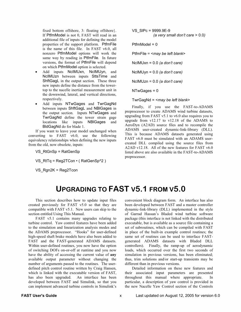
fixed bottom offshore, 3: floating offshore. If PtfmModel is not 0, FAST will read in an additional file of inputs for defining the model properties of the support platform. PtfmFile is the name of this file. In FAST v6.0, all nonzero PtfmModel options will work the same way by reading in PtfmFile. In future versions, the format of PtfmFile will depend on which PtfmModel option is selected.
• Add inputs NcIMUxn, NcIMUyn, and NcIMUzn between inputs SttsTime and ShftGagL in the output section. These three new inputs define the distance from the tower-top to the nacelle inertial measurement unit in the downwind, lateral, and vertical directions, respectively.
• Add inputs NTwGages and TwrGagNd between inputs ShftGagL and NBlGages in the output section. Inputs NTwGages and TwrGagNd define the tower strain gage locations like inputs NBlGages and BldGagNd do for blade 1.
If you want to leave your model unchanged when converting to FAST v6.0, use the following equivalency relationships when defining the new inputs from the old, now obsolete, inputs:
VS_RtGnSp = RatGenSp
VS_RtTq = Reg2TCon • ( RatGenSp^2 )
VS_Rgn2K = Reg2Tcon
VS_SlPc = 9999.9E-9 (a very small don’t care > 0.0)
PtfmModel = 0
PtfmFile = <may be left blank>
NcIMUxn = 0.0 (a don’t care)
NcIMUyn = 0.0 (a don’t care)
NcIMUzn = 0.0 (a don’t care)
NTwGages = 0
TwrGagNd = <may be left blank>
Finally, if you use the FAST-to-ADAMS preprocessor to create ADAMS wind turbine datasets, upgrading from FAST v5.1 to v6.0 also requires you to upgrade from v12.17 to v12.18 of the ADAMS to AeroDyn (A2AD) source files and to recompile the ADAMS user-created dynamic-link-library (DLL). This is because ADAMS datasets generated using FAST v6.0 must be simulated with an ADAMS user-created DLL compiled using the source files from A2AD v12.18. All of the new features for FAST v6.0 listed above are also available in the FAST-to-ADAMS preprocessor.
UPGRADING TO FAST V5.1 FROM V5.0 This section describes how to update input files
created previously for FAST v5.0 so that they are compatible with FAST v5.1. New users can skip to the section entitled Using This Manual.
FAST v5.1 contains many upgrades relating to turbine control. Yaw control features have been added to the simulation and linearization analysis modes and the ADAMS preprocessor. “Hooks” for user-defined high-speed shaft brake models have also been added to FAST and the FAST-generated ADAMS datasets. Within user-defined routines, you now have the option of switching DOFs on-or-off at runtime and you now have the ability of accessing the current value of any available output parameter without changing the number of arguments passed to the routines. The user-defined pitch control routine written by Craig Hansen, which is linked with the executable version of FAST, has also been upgraded. An interface has been developed between FAST and Simulink, so that you can implement advanced turbine controls in Simulink’s
convenient block diagram form. An interface has also been developed between FAST and a master controller dynamic-link-library (DLL) implemented in the style of Garrad Hassan’s Bladed wind turbine software package (this interface is not linked with the distributed executable, but is available as a source file containing a set of subroutines, which can be compiled with FAST in place of the built-in example control routines; the same set of routines can be used to interface FAST-generated ADAMS datasets with Bladed DLL controllers). Finally, the ramp-up of aerodynamic loads, which occurred over the first two seconds of simulation in previous versions, has been eliminated; thus, trim solutions and/or start-up transients may be different than in previous versions.
Detailed information on these new features and their associated input parameters are presented throughout this manual where appropriate. In particular, a description of yaw control is provided in the new Nacelle Yaw Control section of the Controls
FAST User's Guide xi Last updated on August 12, 2005 for version 6.0
chapter, user-defined high-speed shaft brake control is described in the HSS Brake Control section of the Controls chapter, master controller DLLs are described in the Master Controllers and the Bladed-Style DLL Interface section of the Controls chapter, upgrades to Craig’s pitch controller should be apparent by examining the example Pitch.ipt input file located in FAST’s CertTest folder, and a description of FAST’s new interface to Simulink is given in the new Simulink Interface chapter.
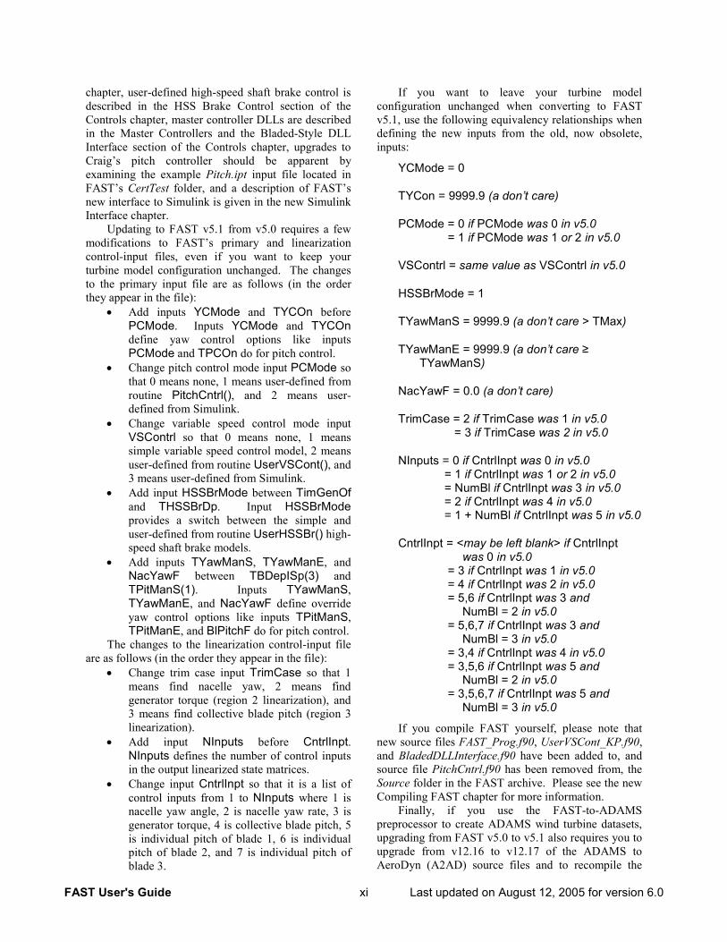
Updating to FAST v5.1 from v5.0 requires a few modifications to FAST’s primary and linearization control-input files, even if you want to keep your turbine model configuration unchanged. The changes to the primary input file are as follows (in the order they appear in the file):
• Add inputs YCMode and TYCOn before PCMode. Inputs YCMode and TYCOn define yaw control options like inputs PCMode and TPCOn do for pitch control.
• Change pitch control mode input PCMode so that 0 means none, 1 means user-defined from routine PitchCntrl(), and 2 means user-defined from Simulink.
• Change variable speed control mode input VSContrl so that 0 means none, 1 means simple variable speed control model, 2 means user-defined from routine UserVSCont(), and 3 means user-defined from Simulink.
• Add input HSSBrMode between TimGenOf and THSSBrDp. Input HSSBrMode provides a switch between the simple and user-defined from routine UserHSSBr() high-speed shaft brake models.
• Add inputs TYawManS, TYawManE, and NacYawF between TBDepISp(3) and TPitManS(1). Inputs TYawManS, TYawManE, and NacYawF define override yaw control options like inputs TPitManS, TPitManE, and BlPitchF do for pitch control.
The changes to the linearization control-input file are as follows (in the order they appear in the file):
• Change trim case input TrimCase so that 1 means find nacelle yaw, 2 means find generator torque (region 2 linearization), and 3 means find collective blade pitch (region 3 linearization).
• Add input NInputs before CntrlInpt. NInputs defines the number of control inputs in the output linearized state matrices.
• Change input CntrlInpt so that it is a list of control inputs from 1 to NInputs where 1 is nacelle yaw angle, 2 is nacelle yaw rate, 3 is generator torque, 4 is collective blade pitch, 5 is individual pitch of blade 1, 6 is individual pitch of blade 2, and 7 is individual pitch of blade 3.
If you want to leave your turbine model configuration unchanged when converting to FAST v5.1, use the following equivalency relationships when defining the new inputs from the old, now obsolete, inputs:
YCMode = 0
TYCon = 9999.9 (a don’t care)
PCMode = 0 if PCMode was 0 in v5.0 = 1 if PCMode was 1 or 2 in v5.0
VSContrl = same value as VSContrl in v5.0
HSSBrMode = 1
TYawManS = 9999.9 (a don’t care > TMax)
TYawManE = 9999.9 (a don’t care ≥ TYawManS)
NacYawF = 0.0 (a don’t care)
TrimCase = 2 if TrimCase was 1 in v5.0 = 3 if TrimCase was 2 in v5.0
NInputs = 0 if CntrlInpt was 0 in v5.0 = 1 if CntrlInpt was 1 or 2 in v5.0 = NumBl if CntrlInpt was 3 in v5.0 = 2 if CntrlInpt was 4 in v5.0 = 1 + NumBl if CntrlInpt was 5 in v5.0
CntrlInpt = <may be left blank> if CntrlInpt was 0 in v5.0
= 3 if CntrlInpt was 1 in v5.0 = 4 if CntrlInpt was 2 in v5.0 = 5,6 if CntrlInpt was 3 and
NumBl = 2 in v5.0 = 5,6,7 if CntrlInpt was 3 and
NumBl = 3 in v5.0 = 3,4 if CntrlInpt was 4 in v5.0 = 3,5,6 if CntrlInpt was 5 and
NumBl = 2 in v5.0 = 3,5,6,7 if CntrlInpt was 5 and
NumBl = 3 in v5.0
If you compile FAST yourself, please note that new source files FAST_Prog.f90, UserVSCont_KP.f90, and BladedDLLInterface.f90 have been added to, and source file PitchCntrl.f90 has been removed from, the Source folder in the FAST archive. Please see the new Compiling FAST chapter for more information.
Finally, if you use the FAST-to-ADAMS preprocessor to create ADAMS wind turbine datasets, upgrading from FAST v5.0 to v5.1 also requires you to upgrade from v12.16 to v12.17 of the ADAMS to AeroDyn (A2AD) source files and to recompile the
FAST User's Guide xii Last updated on August 12, 2005 for version 6.0
ADAMS user-created dynamic-link-library (DLL). This is because ADAMS datasets generated using FAST v5.1 must be simulated with an ADAMS user-created DLL compiled using the source files from
A2AD v12.17. All of the new features for FAST v5.1 listed above are also available in the FAST-to-ADAMS preprocessor.
UPGRADING TO FAST V5.0 FROM V4.4 FAST v5.0 contains a major expansion in the
range of turbine configurations available relative to those available in FAST v4.4. This section describes how to update input files created previously for FAST v4.4 so that they are compatible with FAST v5.0. New users can skip to the section entitled Using This Manual.
New to FAST v5.0 is the availability of a lateral offset and skew angle of the rotor shaft, rotor-furling, tail-furling, and tail inertia and aerodynamics. These new features support the analysis of most small wind turbine configurations. A few new mass and inertia terms are also available for conventional turbine configurations including a yaw bearing point mass, a lateral offset for the nacelle mass, and a hub inertia for 3-bladed rotors (the hub inertia was previously available only for 2-bladed rotor configurations).
While upgrading FAST, we tried to minimize the number of changes to the input files as a courtesy to our users; nevertheless, some changes were unavoidable. Updating to FAST v5.0 from v4.4 requires a few modifications to FAST’s primary and ADAMS-specific input files, even if you want to keep your turbine model configuration unchanged. Additionally, to take advantage of FAST’s new model configuration properties for small wind turbines, a new file of inputs must be assembled. Detailed information on the new features and associated inputs are presented throughout this manual where appropriate. In particular, a description of the input file for specifying additional model properties for a furling turbine is provided in Table 13.
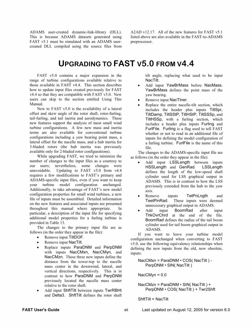
The changes to the primary input file are as follows (in the order they appear in the file):
• Remove input TiltDOF. • Remove input NacTilt. • Replace inputs ParaDNM and PerpDNM
with inputs NacCMxn, NacCMyn, and NacCMzn. These three new inputs define the distance from the tower-top to the nacelle mass center in the downwind, lateral, and vertical directions, respectively. This is in contrast to how ParaDNM and PerpDNM previously located the nacelle mass center relative to the rotor shaft.
• Add input ShftTilt between inputs TwrRBHt and Delta3. ShftTilt defines the rotor shaft
tilt angle, replacing what used to be input NacTilt.
• Add input YawBrMass before NacMass. YawBrMass defines the point mass of the yaw bearing.
• Remove input NacTIner. • Replace the entire nacelle-tilt section, which
includes the header plus inputs TiltSpr, TiltDamp, TiltSStP, TiltHStP, TiltSSSp, and TiltHSSp, with a furling section, which includes a header plus inputs Furling and FurlFile. Furling is a flag used to tell FAST whether or not to read in an additional file of inputs for defining the model configuration of a furling turbine. FurlFile is the name of this file.
The changes to the ADAMS-specific input file are as follows (in the order they appear in the file):
• Add input LSSLength between inputs HSSLength and GenRad. LSSLength defines the length of the low-speed shaft cylinder used for LSS graphical output in ADAMS. This is in contrast to how the LSS previously extended from the hub to the yaw axis.
• Remove inputs TetPnLngth and TeetPinRad. These inputs were deemed unnecessary graphical output in ADAMS.
• Add input BoomRad after input ThkOvrChrd at the end of the file. BoomRad defines the radius of the tail boom cylinder used for tail boom graphical output in ADAMS.
If you want to leave your turbine model configuration unchanged when converting to FAST v5.0, use the following equivalency relationships when defining the new inputs from the old, now obsolete, inputs:
NacCMxn = ParaDNM • COS( NacTilt ) - PerpDNM • SIN( NacTilt )
NacCMyn = 0.0
NacCMzn = ParaDNM • SIN( NacTilt ) + PerpDNM • COS( NacTilt ) + Twr2Shft
ShftTilt = NacTilt
FAST User's Guide xiii Last updated on August 12, 2005 for version 6.0
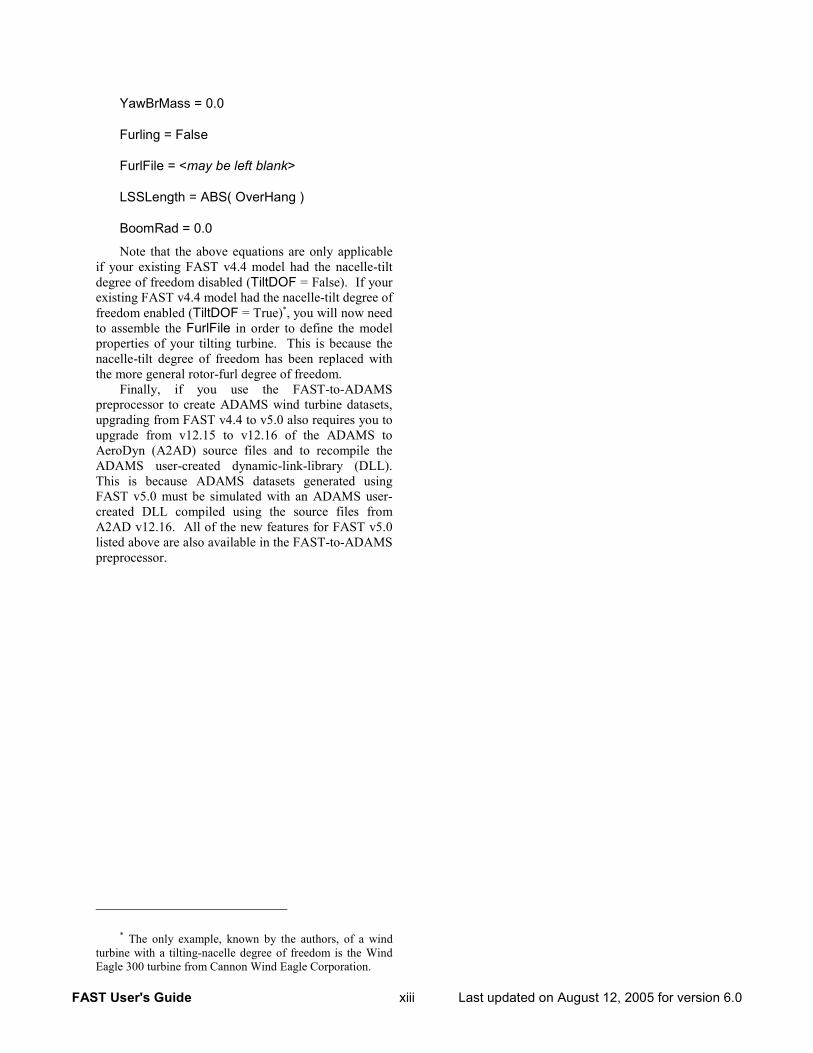
YawBrMass = 0.0
Furling = False
FurlFile = <may be left blank>
LSSLength = ABS( OverHang )
BoomRad = 0.0
Note that the above equations are only applicable if your existing FAST v4.4 model had the nacelle-tilt degree of freedom disabled (TiltDOF = False). If your existing FAST v4.4 model had the nacelle-tilt degree of freedom enabled (TiltDOF = True)*, you will now need to assemble the FurlFile in order to define the model properties of your tilting turbine. This is because the nacelle-tilt degree of freedom has been replaced with the more general rotor-furl degree of freedom.
Finally, if you use the FAST-to-ADAMS preprocessor to create ADAMS wind turbine datasets, upgrading from FAST v4.4 to v5.0 also requires you to upgrade from v12.15 to v12.16 of the ADAMS to AeroDyn (A2AD) source files and to recompile the ADAMS user-created dynamic-link-library (DLL). This is because ADAMS datasets generated using FAST v5.0 must be simulated with an ADAMS user-created DLL compiled using the source files from A2AD v12.16. All of the new features for FAST v5.0 listed above are also available in the FAST-to-ADAMS preprocessor.
* The only example, known by the authors, of a wind turbine with a tilting-nacelle degree of freedom is the Wind Eagle 300 turbine from Cannon Wind Eagle Corporation.
FAST User's Guide xiv Last updated on August 12, 2005 for version 6.0
USING THIS MANUAL We use several typographic conventions in this
manual to make it easy to distinguish various entities. Most titles and headings are formatted with the Arial bold typeface. This manual uses the Times New Roman typeface for body text. To make it easy to spot Variable Names within the body text, we formatted them with the Arial typeface. We did the same for routine names but appended a pair of parentheses to the end of the name (for example, Routine()). We formatted file names with Times New Italic so that we wouldn’t have to deal with the awkward situation of having to include punctuation within the quote marks, which might cause confusion. Examples are formatted with the Letter Gothic typeface.
FAST User's Guide 1 Last updated on August 12, 2005 for version 6.0
MODES OF OPERATION
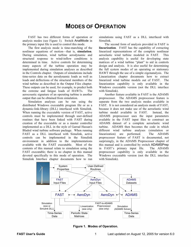
FAST has two different forms of operation or analysis modes (see Figure 1). Switch AnalMode in the primary input file is used to control this mode.
The first analysis mode is time-marching of the nonlinear equations of motion—that is, simulation. During simulation, wind turbine aerodynamic and structural response to wind-inflow conditions is determined in time. Active controls for determining many aspects of the turbine operation may be implemented during simulation analyses as described in the Controls chapter. Outputs of simulations include time-series data on the aerodynamic loads as well as loads and deflections of the structural members of the wind turbine as described in the Output Files chapter. These outputs can be used, for example, to predict both the extreme and fatigue loads of HAWTs. The aerocoustic signature of an operating turbine is another output that can be obtained from simulation.
Simulation analyses can be run using the distributed Windows executable program file or as a dynamic-link-library (DLL) interfaced with Simulink. When running the executable version of FAST, active controls must be implemented through user-defined routines that have been linked with FAST during creation of the executable or as a master controller implemented as a DLL in the style of Garrad Hassan's Bladed wind turbine software package. When running FAST as a DLL interfaced with Simulink, active controls can be implemented in the Simulink environment in addition to the implementations available with the FAST executable. Most of the contents of this manual relate to simulation using the FAST executable; there is no chapter in this manual devoted specifically to this mode of operation. The Simulink Interface chapter documents how to run
simulations using FAST as a DLL interfaced with Simulink.
The second form of analysis provided in FAST is linearization. FAST has the capability of extracting linearized representations of the complete nonlinear aeroelastic wind turbine modeled in FAST. This analysis capability is useful for developing state matrices of a wind turbine “plant” to aid in controls design and analysis. It is also useful for determining the full system modes of an operating or stationary HAWT through the use of a simple eigenanalysis. The Linearization chapter documents how to extract linearized wind turbine models out of FAST. The linearization capability is only available in the Windows executable version (not the DLL interface with Simulink).
Another feature available in FAST is the ADAMS preprocessor. The ADAMS preprocessor feature is separate from the two analysis modes available in FAST. It is not considered an analysis mode of FAST, because it does not make use of the aeroelastic wind turbine model available in FAST. Instead, the ADAMS preprocessor uses the input parameters available in the FAST input files to construct an ADAMS dataset of a complete aeroelastic wind turbine. ADAMS then becomes the code in which different wind turbine analyses (simulation or linearization) are performed. The ADAMS preprocessor feature of FAST is documented, not surprisingly, in the ADAMS Preprocessor chapter of this manual and is controlled by switch ADAMSPrep in FAST’s primary input file. The ADAMS preprocessor capability is only available in the Windows executable version (not the DLL interface with Simulink).
Figure 1. Modes of Operation.
Linearization(exe only)
SystemProperties
FASTInput Files
FAST
Time-SeriesData
Periodic StateMatrices
ADAMSAeroDyn
ADAMSDatasets
Simulation(exe or
Simulink DLL)
AeroDyn
FAST-to-ADAMSPreprocessor
(exe only)
Time-SeriesData
Simulation(ADAMS Solver)
AeroDynInput Files
User-DefinedRoutines
User-DefinedRoutines

FAST User's Guide 3 Last updated on August 12, 2005 for version 6.0
RUNNING FAST
This section documents how to run the FAST Windows executable program file that we distribute in the FAST archive available at our Web page http://wind.nrel.gov/designcodes/simulators/fast/. For a description on how to run FAST with Simulink, see the Simulink Interface chapter.
Before you run FAST, you will want to install it in such a way that you can run it from any folder. For instructions on installing codes such as FAST, please read Buhl (7).
To run the executable, open a command prompt window in the directory in which you want to work. The command-line syntax is:
fast [/h] [<input file>]
where: /h prints a help message. <input file> is the name of the primary input file.
The default name is primary.fst). When FAST runs, it first prints out a line
informing you of the version and compile date of the code. If it cannot find the input file, it aborts with an error message. If it finds a valid input file, FAST
echoes the title line from the input file. If aerodynamic calculations are requested in your input file, the AeroDyn routines then print out some startup messages. If running a time-marching analysis, next, you will see one line that is repeatedly overwritten telling you what the status of the simulation is. It will update this line periodically.
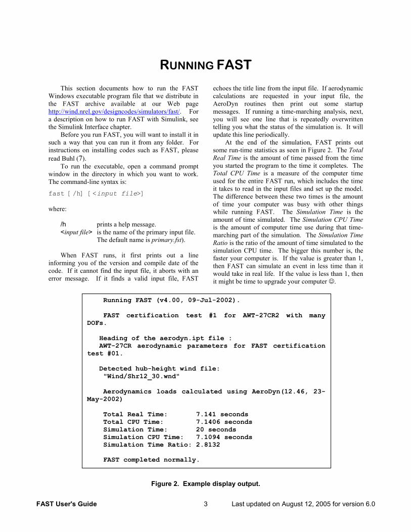
At the end of the simulation, FAST prints out some run-time statistics as seen in Figure 2. The Total Real Time is the amount of time passed from the time you started the program to the time it completes. The Total CPU Time is a measure of the computer time used for the entire FAST run, which includes the time it takes to read in the input files and set up the model. The difference between these two times is the amount of time your computer was busy with other things while running FAST. The Simulation Time is the amount of time simulated. The Simulation CPU Time is the amount of computer time use during that time-marching part of the simulation. The Simulation Time Ratio is the ratio of the amount of time simulated to the simulation CPU time. The bigger this number is, the faster your computer is. If the value is greater than 1, then FAST can simulate an event in less time than it would take in real life. If the value is less than 1, then it might be time to upgrade your computer .
Figure 2. Example display output.
Running FAST (v4.00, 09-Jul-2002). FAST certification test #1 for AWT-27CR2 with many
DOFs. Heading of the aerodyn.ipt file : AWT-27CR aerodynamic parameters for FAST certification
test #01. Detected hub-height wind file: "Wind/Shr12_30.wnd" Aerodynamics loads calculated using AeroDyn(12.46, 23-
May-2002) Total Real Time: 7.141 seconds Total CPU Time: 7.1406 seconds Simulation Time: 20 seconds Simulation CPU Time: 7.1094 seconds Simulation Time Ratio: 2.8132 FAST completed normally.

FAST User's Guide 5 Last updated on August 12, 2005 for version 6.0
COMPILING FAST
You should not need to compile FAST unless you want to create and link a user-defined routine, make changes to the source code, or port FAST to an operating system other than Microsoft Windows. The FAST Windows executable program file that we distribute in the archive can be used for all other purposes.
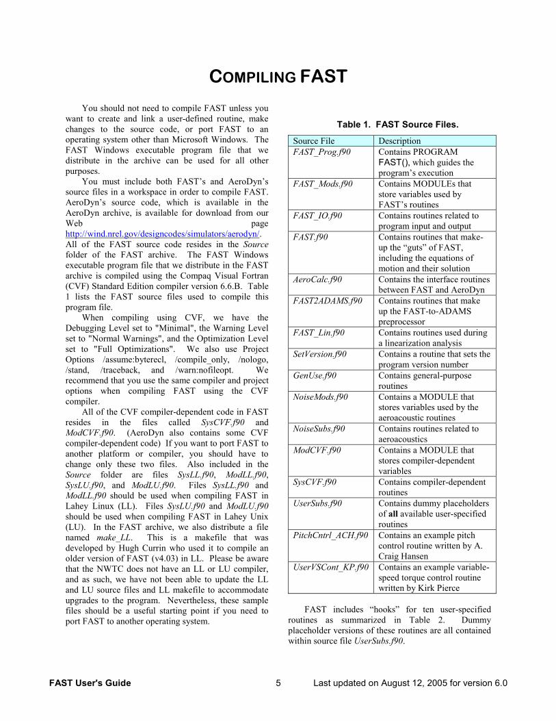
You must include both FAST’s and AeroDyn’s source files in a workspace in order to compile FAST. AeroDyn’s source code, which is available in the AeroDyn archive, is available for download from our Web page http://wind.nrel.gov/designcodes/simulators/aerodyn/. All of the FAST source code resides in the Source folder of the FAST archive. The FAST Windows executable program file that we distribute in the FAST archive is compiled using the Compaq Visual Fortran (CVF) Standard Edition compiler version 6.6.B. Table 1 lists the FAST source files used to compile this program file.
When compiling using CVF, we have the Debugging Level set to "Minimal", the Warning Level set to "Normal Warnings", and the Optimization Level set to "Full Optimizations". We also use Project Options /assume:byterecl, /compile_only, /nologo, /stand, /traceback, and /warn:nofileopt. We recommend that you use the same compiler and project options when compiling FAST using the CVF compiler.
All of the CVF compiler-dependent code in FAST resides in the files called SysCVF.f90 and ModCVF.f90. (AeroDyn also contains some CVF compiler-dependent code) If you want to port FAST to another platform or compiler, you should have to change only these two files. Also included in the Source folder are files SysLL.f90, ModLL.f90, SysLU.f90, and ModLU.f90. Files SysLL.f90 and ModLL.f90 should be used when compiling FAST in Lahey Linux (LL). Files SysLU.f90 and ModLU.f90 should be used when compiling FAST in Lahey Unix (LU). In the FAST archive, we also distribute a file named make_LL. This is a makefile that was developed by Hugh Currin who used it to compile an older version of FAST (v4.03) in LL. Please be aware that the NWTC does not have an LL or LU compiler, and as such, we have not been able to update the LL and LU source files and LL makefile to accommodate upgrades to the program. Nevertheless, these sample files should be a useful starting point if you need to port FAST to another operating system.
Table 1. FAST Source Files.
Source File Description FAST_Prog.f90 Contains PROGRAM
FAST(), which guides the program’s execution
FAST_Mods.f90 Contains MODULEs that store variables used by FAST’s routines
FAST_IO.f90 Contains routines related to program input and output
FAST.f90 Contains routines that make-up the “guts” of FAST, including the equations of motion and their solution
AeroCalc.f90 Contains the interface routines between FAST and AeroDyn
FAST2ADAMS.f90 Contains routines that make up the FAST-to-ADAMS preprocessor
FAST_Lin.f90 Contains routines used during a linearization analysis
SetVersion.f90 Contains a routine that sets the program version number
GenUse.f90 Contains general-purpose routines
NoiseMods.f90 Contains a MODULE that stores variables used by the aeroacoustic routines
NoiseSubs.f90 Contains routines related to aeroacoustics
ModCVF.f90 Contains a MODULE that stores compiler-dependent variables
SysCVF.f90 Contains compiler-dependent routines
UserSubs.f90 Contains dummy placeholders of all available user-specified routines
PitchCntrl_ACH.f90 Contains an example pitch control routine written by A. Craig Hansen
UserVSCont_KP.f90 Contains an example variable-speed torque control routine written by Kirk Pierce
FAST includes “hooks” for ten user-specified
routines as summarized in Table 2. Dummy placeholder versions of these routines are all contained within source file UserSubs.f90.
FAST User's Guide 6 Last updated on August 12, 2005 for version 6.0
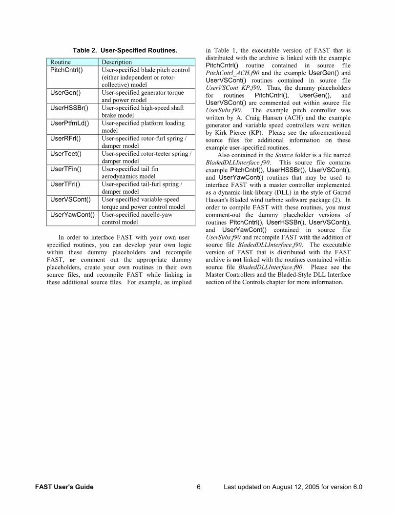
Table 2. User-Specified Routines.
Routine Description PitchCntrl() User-specified blade pitch control
(either independent or rotor-collective) model
UserGen() User-specified generator torque and power model
UserHSSBr() User-specified high-speed shaft brake model
UserPtfmLd() User-specified platform loading model
UserRFrl() User-specified rotor-furl spring / damper model
UserTeet() User-specified rotor-teeter spring / damper model
UserTFin() User-specified tail fin aerodynamics model
UserTFrl() User-specified tail-furl spring / damper model
UserVSCont() User-specified variable-speed torque and power control model
UserYawCont() User-specified nacelle-yaw control model
In order to interface FAST with your own user-
specified routines, you can develop your own logic within these dummy placeholders and recompile FAST, or comment out the appropriate dummy placeholders, create your own routines in their own source files, and recompile FAST while linking in these additional source files. For example, as implied
in Table 1, the executable version of FAST that is distributed with the archive is linked with the example PitchCntrl() routine contained in source file PitchCntrl_ACH.f90 and the example UserGen() and UserVSCont() routines contained in source file UserVSCont_KP.f90. Thus, the dummy placeholders for routines PitchCntrl(), UserGen(), and UserVSCont() are commented out within source file UserSubs.f90. The example pitch controller was written by A. Craig Hansen (ACH) and the example generator and variable speed controllers were written by Kirk Pierce (KP). Please see the aforementioned source files for additional information on these example user-specified routines.
Also contained in the Source folder is a file named BladedDLLInterface.f90. This source file contains example PitchCntrl(), UserHSSBr(), UserVSCont(), and UserYawCont() routines that may be used to interface FAST with a master controller implemented as a dynamic-link-library (DLL) in the style of Garrad Hassan's Bladed wind turbine software package (2). In order to compile FAST with these routines, you must comment-out the dummy placeholder versions of routines PitchCntrl(), UserHSSBr(), UserVSCont(), and UserYawCont() contained in source file UserSubs.f90 and recompile FAST with the addition of source file BladedDLLInterface.f90. The executable version of FAST that is distributed with the FAST archive is not linked with the routines contained within source file BladedDLLInterface.f90. Please see the Master Controllers and the Bladed-Style DLL Interface section of the Controls chapter for more information.
FAST User's Guide 7 Last updated on August 12, 2005 for version 6.0
MODEL DESCRIPTION
General Description The FAST code can model the dynamic response
of both two- and three-bladed, conventional, horizontal-axis wind turbines. The wind turbine configuration may optionally include rotor-furling, tail-furling, and tail aerodynamics—features useful in the analysis of most small wind turbines. The code was evaluated by Germanischer Lloyd WindEnergie and found suitable for "the calculation of onshore wind turbine loads for design and certification" (3).
The FAST model employs a combined modal and multibody dynamics formulation. The model for two-bladed turbines relates nine rigid bodies (earth, support platform, base plate, nacelle, armature, gears, hub, tail, and structure furling with the rotor) and four flexible bodies (tower, two blades, and drive shaft) through 22 degrees of freedom (DOFs). Accounted for in the degrees of freedom are platform translation and rotation (6 DOF), tower flexibility (4 DOF), nacelle yaw (1 DOF), variable generator and rotor speeds (2 DOF), blade teetering (1 DOF), blade flexibility (6 DOF), rotor-furl (1 DOF), and tail-furl (1 DOF). Flexibility in the blades and tower are characterized using a linear modal representation that assumes small deflections. The three rotational DOFs of the support platform (roll, pitch, and yaw) also employ a small angle approximation. The remaining DOFs may exhibit large displacements without loss of accuracy. The DOFs are further described below.
The first six DOFs (the most recent additions) originate from the translational (surge, sway, and heave) and rotational (roll, pitch, and yaw) motions of the support platform relative to the inertia frame.
Two DOFs originate from the first bending mode of the tower in the longitudinal and transverse directions. Two more DOFs model the second bending mode in the same directions. The tower is rigidly attached to the support platform through a cantilever connection.
Another DOF accounts for the nacelle yaw motion, which can be free or fixed with a torsional yaw spring. The rotor can be either upwind or downwind with the rotor providing yaw loads.
The next DOF accounts for variations in generator speed. Another DOF accounts for drivetrain flexibility associated with torsional motion between the generator and the hub/rotor.
Another DOF accounts for teeter motion of the blades about a pin located on the hub. Dampers, springs, or a combination of both can restrict teeter motion.
The next two DOFs arise from the first flapwise bending mode of each blade. Two more DOFs originate from the second flapwise bending modes. Blade edgewise motion accounts for the next two DOFs. The blades are rigidly attached to the hub through a cantilever connection. Motion of the blades is along the local principal axes. See the discussion of blade mode shapes in the Flexible Tower and Blades section on page 10 for details.
The last two DOFs are associated with furling of the rotor and tail about the yawing-portion of the structure atop the tower. The rotor-furl DOF can also be used to model torsional flexibility in the gearbox mounting if you align the rotor-furl axis with the rotor shaft axis. The amount of furling motion can be restricted with springs, dampers, or a combination of both.
The FAST code can also model a three-bladed HAWT with 24 DOFs. The first six DOFs originate from the translational (surge, sway, and heave) and rotational (roll, pitch, and yaw) motions of the support platform relative to the inertia frame. The next four DOFs account for tower motion; two are longitudinal modes, and two are lateral modes. Yawing motion of the nacelle provides another DOF. The next DOF is for the generator azimuth angle, and another DOF is the compliance in the drivetrain between the generator and hub/rotor. These DOFs account for variable rotor speed and drive-shaft flexibility. The next three DOFs are the blade flapwise tip motion for the first mode. Three more DOFs give the tip displacement for each blade for the second flapwise mode. The next three DOFs are for the blade edgewise tip displacement for the first edgewise mode. The last two DOFs are for rotor- and tail-furl.
For both the two- and three-bladed wind turbine configurations, you can enable any combination of the available DOFs and features during your analysis. The DOFs and features most applicable to you are dictated by the configuration of the wind turbine you are analyzing.
Coordinate Systems Figure 3 through Figure 9 show the coordinate
systems used for input and output parameters. Coordinate systems t, n, h, and b conform to the International Electrotechnical Commission (IEC) standard for wind turbines (8). Additional coordinate systems i, p, a, s, and c are necessary for interpreting some of the output parameters. Some of the coordinate systems used internally by FAST differ from these. FAST takes care of these conversions for you.
FAST User's Guide 8 Last updated on August 12, 2005 for version 6.0
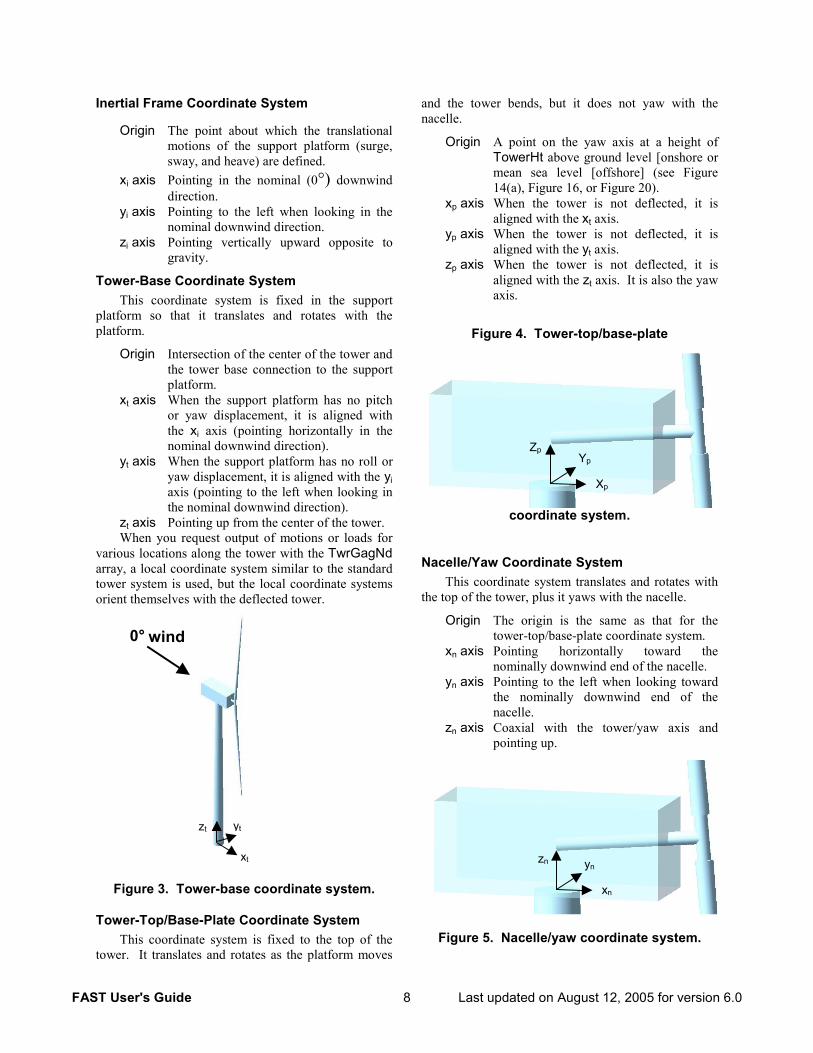
Inertial Frame Coordinate System
Origin The point about which the translational motions of the support platform (surge, sway, and heave) are defined.
xi axis Pointing in the nominal (0°) downwind direction.
yi axis Pointing to the left when looking in the nominal downwind direction.
zi axis Pointing vertically upward opposite to gravity.
Tower-Base Coordinate System This coordinate system is fixed in the support
platform so that it translates and rotates with the platform.
Origin Intersection of the center of the tower and the tower base connection to the support platform.
xt axis When the support platform has no pitch or yaw displacement, it is aligned with the xi axis (pointing horizontally in the nominal downwind direction).
yt axis When the support platform has no roll or yaw displacement, it is aligned with the yi axis (pointing to the left when looking in the nominal downwind direction).
zt axis Pointing up from the center of the tower. When you request output of motions or loads for
various locations along the tower with the TwrGagNd array, a local coordinate system similar to the standard tower system is used, but the local coordinate systems orient themselves with the deflected tower.
Figure 3. Tower-base coordinate system.
Tower-Top/Base-Plate Coordinate System This coordinate system is fixed to the top of the
tower. It translates and rotates as the platform moves
and the tower bends, but it does not yaw with the nacelle.
Origin A point on the yaw axis at a height of TowerHt above ground level [onshore or mean sea level [offshore] (see Figure 14(a), Figure 16, or Figure 20).
xp axis When the tower is not deflected, it is aligned with the xt axis.
yp axis When the tower is not deflected, it is aligned with the yt axis.
zp axis When the tower is not deflected, it is aligned with the zt axis. It is also the yaw axis.
Figure 4. Tower-top/base-plate
coordinate system.
Nacelle/Yaw Coordinate System This coordinate system translates and rotates with
the top of the tower, plus it yaws with the nacelle.
Origin The origin is the same as that for the tower-top/base-plate coordinate system.
xn axis Pointing horizontally toward the nominally downwind end of the nacelle.
yn axis Pointing to the left when looking toward the nominally downwind end of the nacelle.
zn axis Coaxial with the tower/yaw axis and pointing up.
Figure 5. Nacelle/yaw coordinate system.
ZpYp
Xp
zn yn
xn
xt
yt zt
0°
wind
FAST User's Guide 9 Last updated on August 12, 2005 for version 6.0
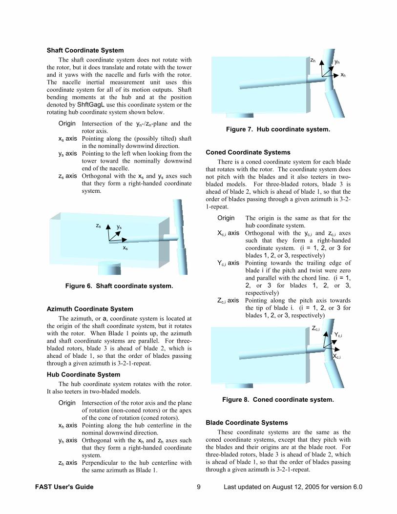
Shaft Coordinate System The shaft coordinate system does not rotate with
the rotor, but it does translate and rotate with the tower and it yaws with the nacelle and furls with the rotor. The nacelle inertial measurement unit uses this coordinate system for all of its motion outputs. Shaft bending moments at the hub and at the position denoted by ShftGagL use this coordinate system or the rotating hub coordinate system shown below.
Origin Intersection of the yn-/zn-plane and the rotor axis.
xs axis Pointing along the (possibly tilted) shaft in the nominally downwind direction.
ys axis Pointing to the left when looking from the tower toward the nominally downwind end of the nacelle.
zs axis Orthogonal with the xs and ys axes such that they form a right-handed coordinate system.
Figure 6. Shaft coordinate system.
Azimuth Coordinate System The azimuth, or a, coordinate system is located at
the origin of the shaft coordinate system, but it rotates with the rotor. When Blade 1 points up, the azimuth and shaft coordinate systems are parallel. For three-bladed rotors, blade 3 is ahead of blade 2, which is ahead of blade 1, so that the order of blades passing through a given azimuth is 3-2-1-repeat.
Hub Coordinate System The hub coordinate system rotates with the rotor.
It also teeters in two-bladed models.
Origin Intersection of the rotor axis and the plane of rotation (non-coned rotors) or the apex of the cone of rotation (coned rotors).
xh axis Pointing along the hub centerline in the nominal downwind direction.
yh axis Orthogonal with the xh and zh axes such that they form a right-handed coordinate system.
zh axis Perpendicular to the hub centerline with the same azimuth as Blade 1.
Figure 7. Hub coordinate system.
Coned Coordinate Systems There is a coned coordinate system for each blade
that rotates with the rotor. The coordinate system does not pitch with the blades and it also teeters in two-bladed models. For three-bladed rotors, blade 3 is ahead of blade 2, which is ahead of blade 1, so that the order of blades passing through a given azimuth is 3-2-1-repeat.
Origin The origin is the same as that for the hub coordinate system.
Xc,i axis Orthogonal with the yc,i and zc,i axes such that they form a right-handed coordinate system. (i = 1, 2, or 3 for blades 1, 2, or 3, respectively)
Yc,i axis Pointing towards the trailing edge of blade i if the pitch and twist were zero and parallel with the chord line. (i = 1, 2, or 3 for blades 1, 2, or 3, respectively)
Zc,i axis Pointing along the pitch axis towards the tip of blade i. (i = 1, 2, or 3 for blades 1, 2, or 3, respectively)
Figure 8. Coned coordinate system.
Blade Coordinate Systems These coordinate systems are the same as the
coned coordinate systems, except that they pitch with the blades and their origins are at the blade root. For three-bladed rotors, blade 3 is ahead of blade 2, which is ahead of blade 1, so that the order of blades passing through a given azimuth is 3-2-1-repeat.
zs ys
xs
xh
yhzh
Xc,i
Yc,i Zc,i
FAST User's Guide 10 Last updated on August 12, 2005 for version 6.0
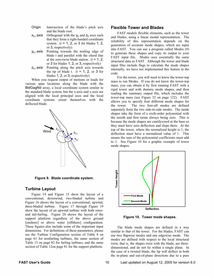
Origin Intersection of the blade’s pitch axis and the blade root.
xb,i axis Orthogonal with the yb and zb axes such that they form a right-handed coordinate system. (i = 1, 2, or 3 for blades 1, 2, or 3, respectively)
yb,i axis Pointing towards the trailing edge of blade i and parallel with the chord line at the zero-twist blade station. (i = 1, 2, or 3 for blades 1, 2, or 3, respectively)
zb,i axis Pointing along the pitch axis towards the tip of blade i. (i = 1, 2, or 3 for blades 1, 2, or 3, respectively)
When you request output of motions or loads for various span locations along the blade with the BldGagNd array, a local coordinate system similar to the standard blade system, but the x-axis and y-axis are aligned with the local principal axes and the local coordinate systems orient themselves with the deflected blade.
Windzb,i
yb,i
xb,i
Figure 9. Blade coordinate system.
Turbine Layout Figure 14 and Figure 15 show the layout of a
conventional, downwind, two-bladed turbine and Figure 16 shows the layout of a conventional, upwind, three-bladed turbine. Figure 17 through Figure 19 show the layout of an upwind turbine with both rotor- and tail-furling. Figure 20 shows the layout of the support platform regardless of the above ground [onshore] or above water [offshore] configuration. These figures also include some of the important input dimensions. For definitions of these parameters, please see the Turbine Configuration section of Table 8 on page 61 for nonfurling turbines, the same section of Table 13 on page 82 for furling turbines, and the same section of Table 12on page 81 for the support platform.
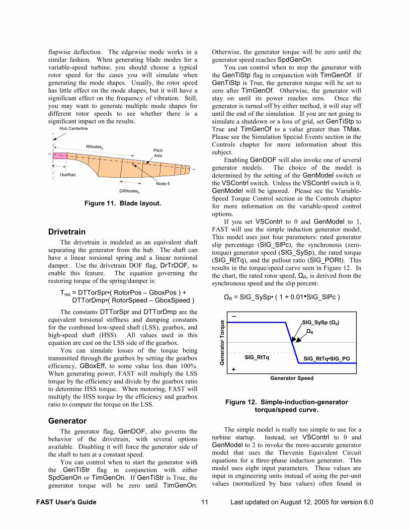
Flexible Tower and Blades FAST models flexible elements, such as the tower
and blades, using a linear modal representation. The reliability of this representation depends on the generation of accurate mode shapes, which are input into FAST. You can use a program called Modes (9) to generate these shapes and copy its output to your FAST input file. Modes uses essentially the same structural data as FAST. Although the tower and blade input files include flags to calculate the mode shapes internally, we have not implemented this feature in the code.
For the tower, you will need to know the tower-top mass to run Modes. If you do not know the tower-top mass, you can obtain it by first running FAST with a rigid tower and with dummy mode shapes, and then reading the summary output file, which includes the tower-top mass (see Figure 32 on page 122). FAST allows you to specify four different mode shapes for the tower. The two fore-aft modes are defined separately from the two side-to-side modes. The mode shapes take the form of a sixth-order polynomial with the zeroth and first terms always being zero. This is because the mode shapes are cantilevered at the base so they must have zero deflection and slope there. At the top of the tower, where the normalized height is 1, the deflection must have a normalized value of 1. This means the sum of the polynomial coefficients must add to 1. See Figure 10 for a graphic example of tower mode shapes.
Deflection
Tow
er H
eigh
t
First Mode
Second Mode
Figure 10. Tower mode shapes.
The blade mode shapes are defined in a way similar to that of the tower. For the blades, FAST can use two flapwise modes and one edgewise mode. The modes are defined with respect to the local structural twist, that is, the shapes twist with the blade, are three-dimensional, and do not lie within a single plane. In the case of a twisted blade, the tip will deflect in both the in-plane and out-of-plane directions due to a pure
FAST User's Guide 11 Last updated on August 12, 2005 for version 6.0
flapwise deflection. The edgewise mode works in a similar fashion. When generating blade modes for a variable-speed turbine, you should choose a typical rotor speed for the cases you will simulate when generating the mode shapes. Usually, the rotor speed has little effect on the mode shapes, but it will have a significant effect on the frequency of vibration. Still, you may want to generate multiple mode shapes for different rotor speeds to see whether there is a significant impact on the results.
HubRad
RNodes5
DRNodes5
Hub Centerline
PitchAxis
Node 5
Figure 11. Blade layout.
Drivetrain The drivetrain is modeled as an equivalent shaft
separating the generator from the hub. The shaft can have a linear torsional spring and a linear torsional damper. Use the drivetrain DOF flag, DrTrDOF, to enable this feature. The equation governing the restoring torque of the spring/damper is:
Tres = DTTorSpr•( RotorPos – GboxPos ) + DTTorDmp•( RotorSpeed – GboxSpeed )
The constants DTTorSpr and DTTorDmp are the equivalent torsional stiffness and damping constants for the combined low-speed shaft (LSS), gearbox, and high-speed shaft (HSS). All values used in this equation are cast on the LSS side of the gearbox.
You can simulate losses of the torque being transmitted through the gearbox by setting the gearbox efficiency, GBoxEff, to some value less than 100%. When generating power, FAST will multiply the LSS torque by the efficiency and divide by the gearbox ratio to determine HSS torque. When motoring, FAST will multiply the HSS torque by the efficiency and gearbox ratio to compute the torque on the LSS.
Generator The generator flag, GenDOF, also governs the
behavior of the drivetrain, with several options available. Disabling it will force the generator side of the shaft to turn at a constant speed.
You can control when to start the generator with the GenTiStr flag in conjunction with either SpdGenOn or TimGenOn. If GenTiStr is True, the generator torque will be zero until TimGenOn.
Otherwise, the generator torque will be zero until the generator speed reaches SpdGenOn.
You can control when to stop the generator with the GenTiStp flag in conjunction with TimGenOf. If GenTiStp is True, the generator torque will be set to zero after TimGenOf. Otherwise, the generator will stay on until its power reaches zero. Once the generator is turned off by either method, it will stay off until the end of the simulation. If you are not going to simulate a shutdown or a loss of grid, set GenTiStp to True and TimGenOf to a value greater than TMax. Please see the Simulation Special Events section in the Controls chapter for more information about this subject.
Enabling GenDOF will also invoke one of several generator models. The choice of the model is determined by the setting of the GenModel switch or the VSContrl switch. Unless the VSContrl switch is 0, GenModel will be ignored. Please see the Variable-Speed Torque Control section in the Controls chapter for more information on the variable-speed control options.
If you set VSContrl to 0 and GenModel to 1, FAST will use the simple induction generator model. This model uses just four parameters: rated generator slip percentage (SIG_SlPc), the synchronous (zero-torque) generator speed (SIG_SySp), the rated torque (SIG_RtTq), and the pullout ratio (SIG_PORt). This results in the torque/speed curve seen in Figure 12. In the chart, the rated rotor speed, ΩR, is derived from the synchronous speed and the slip percent:
ΩR = SIG_SySp• ( 1 + 0.01•SIG_SlPc )
Generator Speed
Gen
erat
or T
orqu
e
ΩR
SIG_SySp (Ω0)
SIG_RtTq SIG_RtTq•SIG_PO
–
+
Figure 12. Simple-induction-generator torque/speed curve.
The simple model is really too simple to use for a turbine startup. Instead, set VSContrl to 0 and GenModel to 2 to invoke the more-accurate generator model that uses the Thevenin Equivalent Circuit equations for a three-phase induction generator. This model uses eight input parameters. These values are input in engineering units instead of using the per-unit values (normalized by base values) often found in
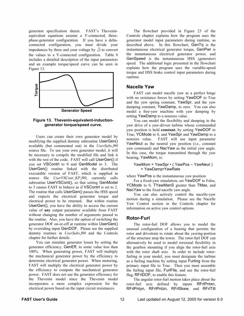
FAST User's Guide 12 Last updated on August 12, 2005 for version 6.0
generator specification sheets. FAST’s Thevenin-equivalent equations assume a Y-connected, three-phase-generator configuration. If you have a delta-connected configuration, you must divide your impedances by three and your voltage by 3 to convert the values to a Y-connected configuration. Table 8 includes a detailed description of the input parameters and an example torque/speed curve can be seen in Figure 13.
Generator Speed
Torq
ue
Figure 13. Thevenin-equivalent-induction-
generator torque/speed curve.
Users can create their own generator model by modifying the supplied dummy subroutine UserGen() available (but commented out) in the UserSubs.f90 source file. To use your own generator model, it will be necessary to compile the modified file and link it with the rest of the code. FAST will call UserGen() if you set VSContrl to 0 and GenModel to 3. The UserGen() routine linked with the distributed executable version of FAST, which is supplied in source file UserVSCont_KP.f90, currently calls subroutine UserVSCont(), so that setting GenModel to 3 causes FAST to behave as if VSContrl is set to 2. The routine that calls UserGen() passes the HSS speed and expects the electrical generator torque and electrical power to be returned. But within routine UserGen(), you have the ability to access the current value of any output parameter available from FAST without changing the number of arguments passed to the routine. Also, you have the option of switching the generator DOF on-or-off at runtime within UserGen() by overriding input GenDOF. Please see the supplied dummy routines in UserSubs.f90 and the Controls chapter for further details.
You can simulate generator losses by setting the generator efficiency, GenEff, to some value less than 100%. When generating power, FAST will multiply the mechanical generator power by the efficiency to determine electrical generator power. When motoring, FAST will multiply the electrical generator power by the efficiency to compute the mechanical generator power. FAST does not use the generator efficiency for the Thevenin model since the Thevenin model incorporates a more complex expression for the electrical power based on the input circuit resistances.
The flowchart provided in Figure 23 of the Controls chapter explains how the program uses the generator model input parameters during runtime, as described above. In this flowchart, GenTq is the instantaneous electrical generator torque, GenPwr is the instantaneous electrical generator power, and GenSpeed is the instantaneous HSS (generator) speed. The additional logic presented in the flowchart explains how the program uses the variable-speed torque and HSS brake control input parameters during runtime.
Nacelle Yaw FAST can model nacelle yaw as a perfect hinge
with no resistance forces by setting YawDOF to True and the yaw spring constant, YawSpr, and the yaw damping constant, YawDamp, to zero. You can also model a free-yaw machine with yaw damping by setting YawDamp to a nonzero value.
You can model the flexibility and damping in the yaw drive of a yaw-driven turbine whose commanded yaw position is held constant, by setting YawDOF to True, YCMode to 0, and YawSpr and YawDamp to a nonzero value. FAST will use input parameter YawNeut as the neutral yaw position (i.e., constant yaw command) and NacYaw as the initial yaw angle. In this case, the torque transmitted through the yaw bearing, YawMom, is:
YawMom = YawSpr • ( YawPos – YawNeut ) + YawDamp•YawRate
where YawPos is the instantaneous yaw position. For a fixed-yaw simulation, set YawDOF to False,
YCMode to 0, TYawManS greater than TMax, and NacYaw to the fixed nacelle yaw angle.
You can also actively control the nacelle-yaw motion during a simulation. Please see the Nacelle Yaw Control section in the Controls chapter for information on active yaw control options.
Rotor-Furl The rotor-furl DOF allows you to model the
unusual configuration of a bearing that permits the rotor and drivetrain to rotate about the yawing-portion of the structure atop the tower. The rotor-furl DOF can alternatively be used to model torsional flexibility in the gearbox mounting if you align the rotor-furl axis with the rotor shaft axis. In order to include rotor-furling in your model, you must designate the turbine as a furling machine by setting input Furling from the primary input file to True. Then you must assemble the furling input file, FurlFile, and use the rotor-furl flag, RFrlDOF, to enable this feature.
The angular rotor-furl motion takes place about the rotor-furl axis defined by inputs RFrlPntxn, RFrlPntyn, RFrlPntzn, RFrlSkew, and RFrlTilt
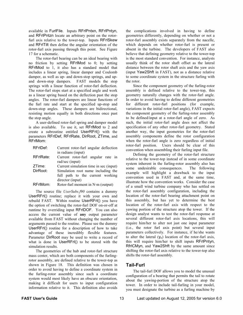
FAST User's Guide 13 Last updated on August 12, 2005 for version 6.0
available in FurlFile. Inputs RFrlPntxn, RFrlPntyn, and RFrlPntzn locate an arbitrary point on the rotor-furl axis relative to the tower-top. Inputs RFrlSkew and RFrlTilt then define the angular orientation of the rotor-furl axis passing through this point. See Figure 17 for a schematic.
The rotor-furl bearing can be an ideal bearing with no friction by setting RFrlMod to 0; by setting RFrlMod to 1, it also has a standard model that includes a linear spring, linear damper and Coulomb damper, as well as up- and down-stop springs, and up- and down-stop dampers. FAST models the stop springs with a linear function of rotor-furl deflection. The rotor-furl stops start at a specified angle and work as a linear spring based on the deflection past the stop angles. The rotor-furl dampers are linear functions of the furl rate and start at the specified up-stop and down-stop angles. These dampers are bidirectional, resisting motion equally in both directions once past the stop angle.
A user-defined rotor-furl spring and damper model is also available. To use it, set RFrlMod to 2 and create a subroutine entitled UserRFrl() with the parameters RFrlDef, RFrlRate, DirRoot, ZTime, and RFrlMom:
RFrlDef: Current rotor-furl angular deflection in radians (input)
RFrlRate: Current rotor-furl angular rate in rad/sec (input)
ZTime: Current simulation time in sec (input) DirRoot: Simulation root name including the
full path to the current working director (input)
RFrlMom: Rotor-furl moment in N·m (output)
The source file UserSubs.f90 contains a dummy UserRFrl() routine; replace it with your own and rebuild FAST. Within routine UserRFrl() you have the option of switching the rotor-furl DOF on-or-off at runtime by overriding input RFrlDOF. You can also access the current value of any output parameter available from FAST without changing the number of arguments passed to the routine. Please see the dummy UserRFrl() routine for a description of how to take advantage of these incredibly flexible features. Parameter DirRoot may be used to write a record of what is done in UserRFrl() to be stored with the simulation results.
The geometries of the hub and rotor-furl structure mass center, which are both components of the furling-rotor assembly, are defined relative to the tower-top as shown in Figure 18. This definition was chosen in order to avoid having to define a coordinate system in the furling-rotor assembly since such a coordinate system would most likely have an obscure orientation, making it difficult for users to input configuration information relative to it. This definition also avoids
the complications involved in having to define geometries differently, depending on whether or not a rotor-furl assembly exists separately from the nacelle, which depends on whether rotor-furl is present or absent in the turbine. The developers of FAST also believe that defining geometry relative to the tower-top is the most standard convention. For instance, analysts usually think of the rotor shaft offset as the lateral distance between the rotor shaft axis and the yaw axis (input Yaw2Shft in FAST), not as a distance relative to some coordinate system in the structure furling with the rotor.
Since the component geometry of the furling-rotor assembly is defined relative to the tower-top, this geometry naturally changes with the rotor-furl angle. In order to avoid having to define different geometries for different rotor-furl positions (for example, variations in the initial rotor-furl angle), FAST expects the component geometry of the furling-rotor assembly to be defined/input at a rotor-furl angle of zero. As such, the initial rotor-furl angle does not affect the specification of any other rotor-furl geometry. Stated another way, the input geometries for the rotor-furl assembly components define the rotor configuration when the rotor-furl angle is zero regardless of initial rotor-furl position. Users should be clear of this convention when assembling their furling input file.
Defining the geometry of the rotor-furl structure relative to the tower-top instead of in some coordinate system inherent in the furling-rotor assembly also has some undesirable consequences. The following example will highlight a drawback to the input convention used in FAST and, at the same time, illustrate how the convention works. Consider the case of a small wind turbine company who has settled on the rotor-furl assembly configuration, including the location of the rotor-furl bearing attachment point on this assembly, but has yet to determine the best location of the rotor-furl axis with respect to the yawing portion of the structure atop the tower. If the design analyst wants to test the rotor-furl response at several different rotor-furl axis locations, this will require him/her to alter not just one input parameter (i.e., the rotor furl axis point) but several input parameters collectively. For instance, if he/she wants to alter the lateral (yn) location of the rotor-furl axis, this will require him/her to shift inputs RFrlPntyn, RfrlCMyn, and Yaw2Shft by the same amount since shifting the rotor-furl axis relative to the tower-top also shifts the rotor-furl assembly.
Tail-Furl The tail-furl DOF allows you to model the unusual
configuration of a bearing that permits the tail to rotate about the yawing-portion of the structure atop the tower. In order to include tail-furling in your model, you must designate the turbine as a furling machine by
FAST User's Guide 14 Last updated on August 12, 2005 for version 6.0
setting input Furling from the primary input file to True. Then you must assemble the furling input file, FurlFile, and use the tail-furl flag, TFrlDOF, to enable this feature.
The angular tail-furl motion takes place about the tail-furl axis defined by inputs TFrlPntxn, TFrlPntyn, TFrlPntzn, TFrlSkew, and TFrlTilt available in FurlFile. Inputs TFrlPntxn, TFrlPntyn, and TFrlPntzn locate an arbitrary point on the tail-furl axis relative to the tower-top. Inputs TFrlSkew and TFrlTilt then define the angular orientation of the tail-furl axis passing through this point. See Figure 17 for a schematic.
The tail-furl bearing can be an ideal bearing with no friction by setting TFrlMod to 0; by setting TFrlMod to 1, it also has a standard model that includes a linear spring, linear damper and Coulomb damper, as well as up- and down-stop springs, and up- and down-stop dampers. FAST models the stop springs with a linear function of tail-furl deflection. The tail-furl stops start at a specified angle and work as a linear spring based on the deflection past the stop angles. The tail-furl dampers are linear functions of the furl rate and start at the specified up-stop and down-stop angles. These dampers are bidirectional, resisting motion equally in both directions once past the stop angle.
A user-defined tail-furl spring and damper model is also available. To use it, set TFrlMod to 2 and create a subroutine entitled UserTFrl() with the parameters TFrlDef, TFrlRate, ZTime, DirRoot, and TFrlMom:
TFrlDef: Current tail-furl angular deflection in radians (input)
TFrlRate: Current tail-furl angular rate in rad/sec (input)
ZTime: Current simulation time in sec (input) DirRoot: Simulation root name including the
full path to the current working director (input)
TFrlMom: Tail-furl moment in N·m (output)
The source file UserSubs.f90 contains a dummy UserTFrl() routine; replace it with your own and rebuild FAST. Within routine UserTFrl() you have the option of switching the tail-furl DOF on-or-off at runtime by overriding input TFrlDOF. You can also access the current value of any output parameter available from FAST without changing the number of arguments passed to the routine. Please see the dummy UserTFrl() routine for a description of how to take advantage of these incredibly flexible features. Parameter DirRoot may be used to write a record of what is done in UserTFrl() to be stored with the simulation results.
The geometries of the tail boom mass center, tail fin mass center, and tail fin aerodynamic surface,
which are all components of the furling-tail assembly, are defined relative to the tower-top as shown in Figure 19. This definition was chosen in order to avoid having to define a coordinate system in the furling-tail assembly since such a coordinate system would most likely have an obscure orientation, making it difficult for users to input configuration information relative to it. This definition also avoids the complications involved in having to define geometries differently, depending on whether or not a tail-furl assembly exists separately from the nacelle, which depends on whether tail-furl is present or absent in the turbine.
Since the component geometry of the furling-tail assembly is defined relative to the tower-top, this geometry naturally changes with the tail-furl angle. In order to avoid having to define different geometries for different tail-furl positions (for example, variations in the initial tail-furl angle), FAST expects the component geometry of the furling-tail assembly to be defined/input at a tail-furl angle of zero. As such, the initial tail-furl angle does not affect the specification of any other tail-furl geometry. Stated another way, the input geometries for the tail-furl assembly components define the tail configuration when the tail-furl angle is zero regardless of initial tail-furl position. Users should be clear of this convention when assembling their furling input file. Further clarification on this furling geometry convention is provided in the Rotor-Furl section above.
Rotor-Teeter For two-bladed turbines, FAST can model a
teetering rotor. To enable the teeter DOF, set TeetDOF to True.
The teeter bearing can be an ideal bearing with no friction by setting TeetMod to 0; by setting TeetMod to 1, it also has a standard model that includes a spring, stop, and damper. FAST models the spring with a linear function of teeter deflection. The teeter stop starts at a specified angle and works as a linear spring based on the deflection past the stop angle. The teeter damper is a linear function of teeter rate that starts at a specified angle.
A user-defined teeter-spring and damper model is also available. To use it, set TeetMod to 2 and create a subroutine entitled UserTeet() with the parameters TeetDef, TeetRate, ZTime, DirRoot, and TeetMom:
TeetDef: Current teeter deflection in radians (input)
TeetRate: Current teeter rate in rad/sec (input) ZTime: Current simulation time in sec (input) DirRoot: Simulation root name including the
full path to the current working director (input)
TeetMom: Teeter moment in N·m (output)
FAST User's Guide 15 Last updated on August 12, 2005 for version 6.0
The source file UserSubs.f90 contains a dummy UserTeet() routine; replace it with your own and rebuild FAST. Within routine UserTeet() you have the option of switching the rotor-teeter DOF on-or-off at runtime by overriding input TeetDOF. You can also access the current value of any output parameter available from FAST without changing the number of arguments passed to the routine. Please see the dummy UserTeet() routine for a description of how to take advantage of these incredibly flexible features. Parameter DirRoot may be used to write a record of what is done in UserTeet() to be stored with the simulation results.
FAST also allows you to specify a δ3 angle for the teeter hinge. By teetering about an angle that is not perpendicular to the blades, you can introduce flap/pitch coupling to your rotor. This is thought to add aerodynamic restoring forces to the blade. Positive δ3 will cause the leading edge of the downwind-most blade to feather into the wind. This is illustrated in Figure 15. See Malcolm’s paper (10) for an analysis of δ3.
Support Platform You can model the support platform in an onshore
foundation, fixed bottom offshore foundation, or floating offshore configuration by setting the value of input switch PtfmModel from the primary input file to 1, 2, or 3, respectively. Setting PtfmModel to 0 disables the platform models—in this case, FAST will rigidly attach the tower to the inertia frame (ground) through a cantilever connection.
The support platform model properties are designated using the input parameters available in the platform input file, PtfmFile. In FAST v6.0, all nonzero PtfmModel options work the same way by reading in PtfmFile. In future versions, the format of this file will depend on which PtfmModel option is selected.
A layout of the configuration properties available for the support platform is given in Figure 20. The platform reference point, located by input parameter PtfmRef, is the origin in the platform about which the translational (surge, sway, and heave) and rotational (roll, pitch, and yaw) motions of the support platform are defined. It is also the point at which external loading is applied to the platform.
In FAST v6.0, only user-defined platform loading is available. For a value of 0 for PtfmLdMod (available in PtfmFile), there will be no platform loading and the support reactions normally produced will be set to zero (causing the wind turbine to fall due to gravity if PtfmHvDOF is True).
If you set PtfmLdMod to 1, FAST will call a user defined routine named UserPtfmLd() to compute the platform loading. The platform loads returned by UserPtfmLd() should contain contributions from any
external load acting on the platform other than loads transmitted from the wind turbine. For example, these loads should contain contributions from foundation stiffness and damping [not floating] or mooring line restoring and damping [floating], as well as hydrostatic and hydrodynamic contributions [offshore]. The platform loads will be applied on the platform at the instantaneous platform reference position (located by input PtfmRef).
To use this feature, set PtfmLdMod to 1 and create a subroutine entitled UserPtfmLd() with the parameters X(6), XD(6), ZTime, DirRoot, PtfmAM(6,6), and PtfmFt(6):
X(6): A vector of size 6 containing the 3 components of the current platform translational displacement in meters and the 3 components of the current platform rotational displacement in radians (input)
XD(6): A vector of size 6 containing the 3 components of the current platform translational velocity in m/sec and the 3 components of the current platform rotational (angular) velocity in rad/sec (input)
ZTime: Current simulation time in sec (input) DirRoot: Simulation root name including the
full path to the current working director (input)
PtfmAM(6,6): A symmetric matrix of size 6 X 6 containing the current added mass matrix of the platform with units of kg, kg·m and kg·m2 (output)
PtfmFt(6): A vector of size 6 containing 3 translational and 3 rotational components of the current portion of the platform load, with units of N and N·m, associated with everything but the added mass effects (output)
As implied by the outputs above, the routine assumes that the platform loads are transmitted through a medium like soil [foundation] and/or water [offshore], so that added mass effects are important. Consequently, the routine assumes that the total platform load can be written as:
PtfmF(i) = SUM( -PtfmAM(i,j)•XDD(j), j = 1,2,…,6) + PtfmFt(i) (for i = 1,2,…,6)
where,
PtfmF(i): The ith component of the total load applied on the platform; positive in the direction of positive motion of the ith DOF of the platform
PtfmAM(i,j): The (i,j) component of the platform added mass matrix
FAST User's Guide 16 Last updated on August 12, 2005 for version 6.0
XDD(j): The jth component of the platform acceleration vector
PtfmFt(i): The ith component of the portion of the platform load associated with everything but the added mass effects; positive in the direction of positive motion of the ith DOF of the platform
The order of indices in all arrays passed to and from routine UserPtfmLd() is asfollows:
1 = Platform surge / xi-component of platform translation
2 = Platform sway / yi-component of platform translation
3 = Platform heave / zi-component of platform translation
4 = Platform roll / xi-component of platform rotation
5 = Platform pitch / yi-component of platform rotation
6 = Platform yaw / zi-component of platform rotation
The source file UserSubs.f90 contains a dummy UserPtfmLd() routine; replace it with your own and rebuild FAST. Within routine UserPtfmLd() you have the option of switching the platform DOFs on-or-off at runtime by overriding inputs PtfmSgDOF, PtfmSwDOF, PtfmHvDOF, PtfmRDOF, PtfmPDOF, and PtfmYDOF. You can also access the current value of any output parameter available from FAST without changing the number of arguments passed to the routine. Please see the dummy UserPtfmLd() routine for a description of how to take advantage of these incredibly flexible features. Parameter DirRoot may be used to write a record of what is done in UserPtfmLd() to be stored with the simulation results.
When using UserPtfmLd(), please note that the hydrostatic restoring contribution to the hydrodynamic force returned by the routine should not contain the effects of body weight, as is often done in classical marine hydrodynamics. The effects of body weight are included within FAST and ADAMS.
Rotor Aerodynamics The AeroDyn aerodynamic subroutine library
supplies the aerodynamics algorithms for the rotor. Although we include descriptions of the parameters in the AeroDyn input file in Table 11, please refer to the AeroDyn User’s Guide (1) for most of the details on this package. Input flag CompAero can be used to disable aerodynamics calculations while debugging a model.
Tail Fin Aerodynamics Your model can optionally include tail fin
aerodynamic loads. In order to include them, you must designate the turbine as a furling machine by setting input Furling from the primary input file to True and then assemble the furling input file, FurlFile. A furling model may also exclude tail fin aerodynamic loads by setting TFinMod in FurlFile to 0.
You can choose to invoke a simple tail fin aerodynamics model built into FAST by setting TFinMod to 1. By accessing information from AeroDyn, this model computes the relative velocity of the wind-inflow and its angle of attack relative to the tail fin chordline and uses an AeroDyn airfoil table chosen by the user (TFinNFoil) to determine the lift and drag forces acting at the tail fin center-of-pressure. Set SubAxInd to False if you want the wind velocity at the tail fin to be unobstructed by the rotor wake. Set SubAxInd to True if you want FAST to decrease (i.e., subtract) the wind velocity at the tail fin center-of-pressure by the average rotor induced velocity in the rotor shaft direction.
You also have the option of implementing far more sophisticated tail fin aerodynamics models by supplying your own routines that can easily be linked with the rest of FAST. To do this, set TFinMod to 2 and create a subroutine entitled UserTFin(). The source file UserSubs.f90 contains a dummy UserTFin() routine; replace it with your own and rebuild FAST. The routine that calls UserTFin() passes the tail-furl angle and rate and tail-fin center-of-pressure location and velocity and expects the angle of attack, lift and drag coefficients, local dynamic pressure, as well as the normal and tangential forces to be returned. But within routine UserTFin(), you have the ability to access the current value of any output parameter available from FAST without changing the number of arguments passed to the routine. Please see the supplied dummy routine in UserSubs.f90 for further details.
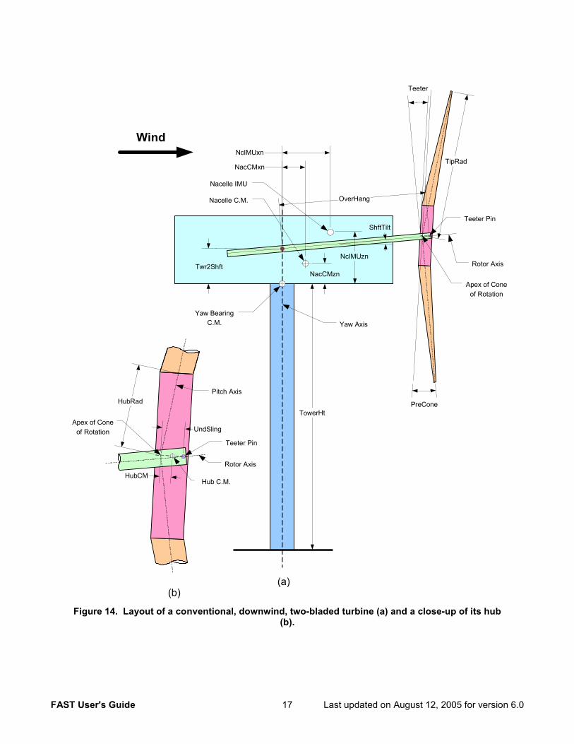
FAST User's Guide 17 Last updated on August 12, 2005 for version 6.0
Figure 14. Layout of a conventional, downwind, two-bladed turbine (a) and a close-up of its hub (b).
Wind
Teeter Pin
UndSling
HubCM
OverHang
Teeter Pin
HubRadPitch Axis
Rotor Axis
TipRad
TowerHtApex of Cone
of Rotation
Hub C.M.
Nacelle C.M.
(a)(b)
PreCone
Teeter
Apex of Coneof Rotation
Yaw Axis
Rotor Axis
Twr2ShftNacCMzn
NacCMxn
ShftTilt
Yaw BearingC.M.
NcIMUzn
NcIMUxn
Nacelle IMU
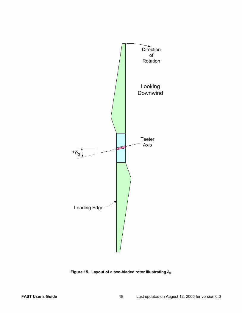
FAST User's Guide 18 Last updated on August 12, 2005 for version 6.0
Figure 15. Layout of a two-bladed rotor illustrating δ3.
TeeterAxis
LookingDownwind
+δ3
Directionof
Rotation
Leading Edge
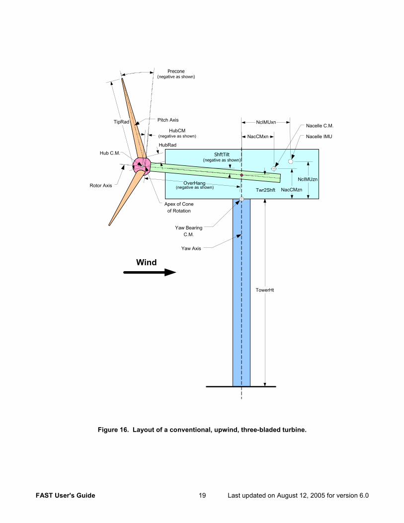
FAST User's Guide 19 Last updated on August 12, 2005 for version 6.0
Figure 16. Layout of a conventional, upwind, three-bladed turbine.
Wind
Rotor Axis
Yaw Axis
TipRad
Precone(negative as shown)
Apex of Coneof Rotation
ShftTilt(negative as shown)
OverHang
Nacelle C.M.
Hub C.M.
HubCM(negative as shown)
Pitch Axis
HubRad
TowerHt
(negative as shown) Twr2Shft
Yaw BearingC.M.
NacCMzn
NacCMxn
NcIMUzn
NcIMUxn
Nacelle IMU
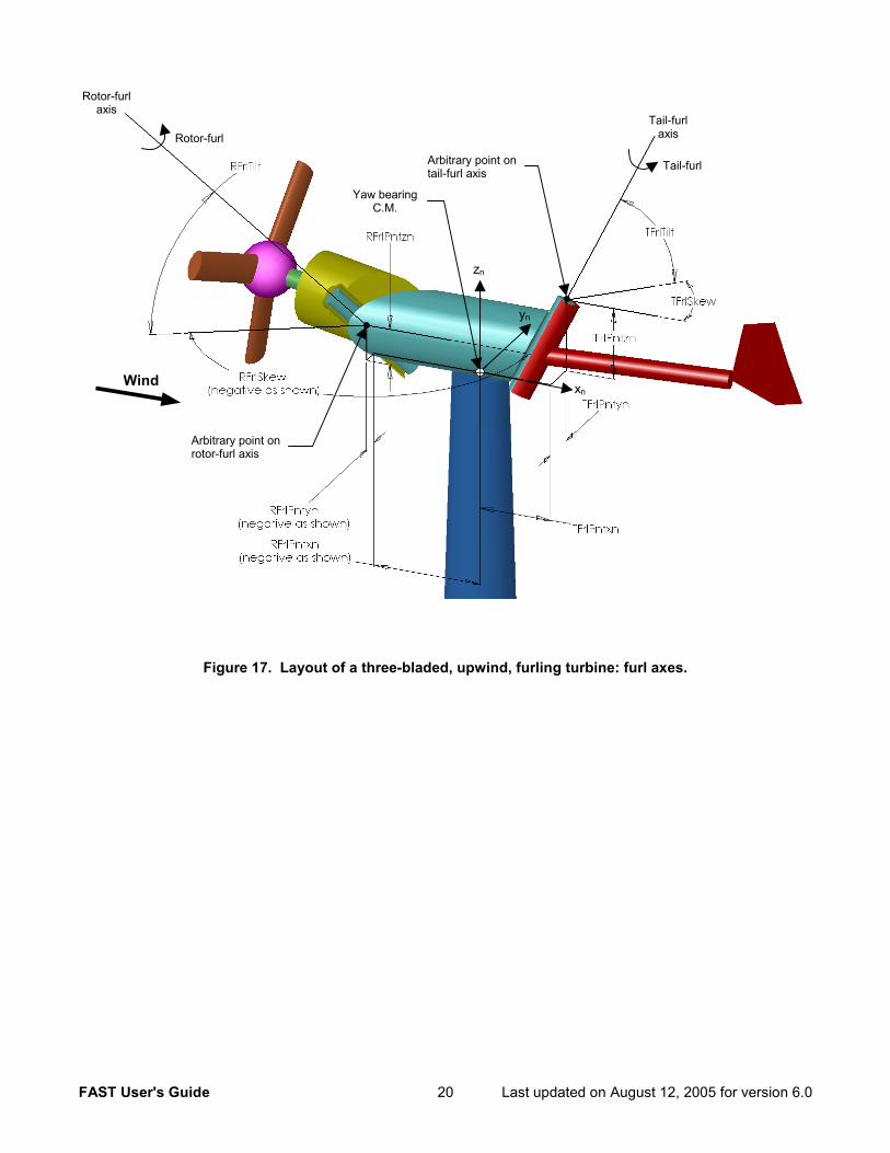
FAST User's Guide 20 Last updated on August 12, 2005 for version 6.0
Figure 17. Layout of a three-bladed, upwind, furling turbine: furl axes.
zn
yn
xn
Tail-furl axis
Arbitrary point on rotor-furl axis
Arbitrary point on tail-furl axis
Rotor-furl axis
Yaw bearing C.M.
Rotor-furl
Tail-furl
Wind
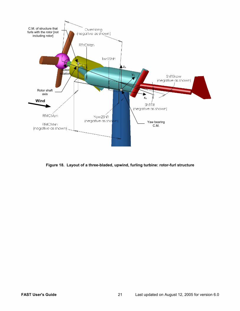
FAST User's Guide 21 Last updated on August 12, 2005 for version 6.0
Figure 18. Layout of a three-bladed, upwind, furling turbine: rotor-furl structure
zn
yn
xn
Rotor shaft axis
C.M. of structure that furls with the rotor [not
including rotor]
Rotor rotation
Wind
Yaw bearing C.M.
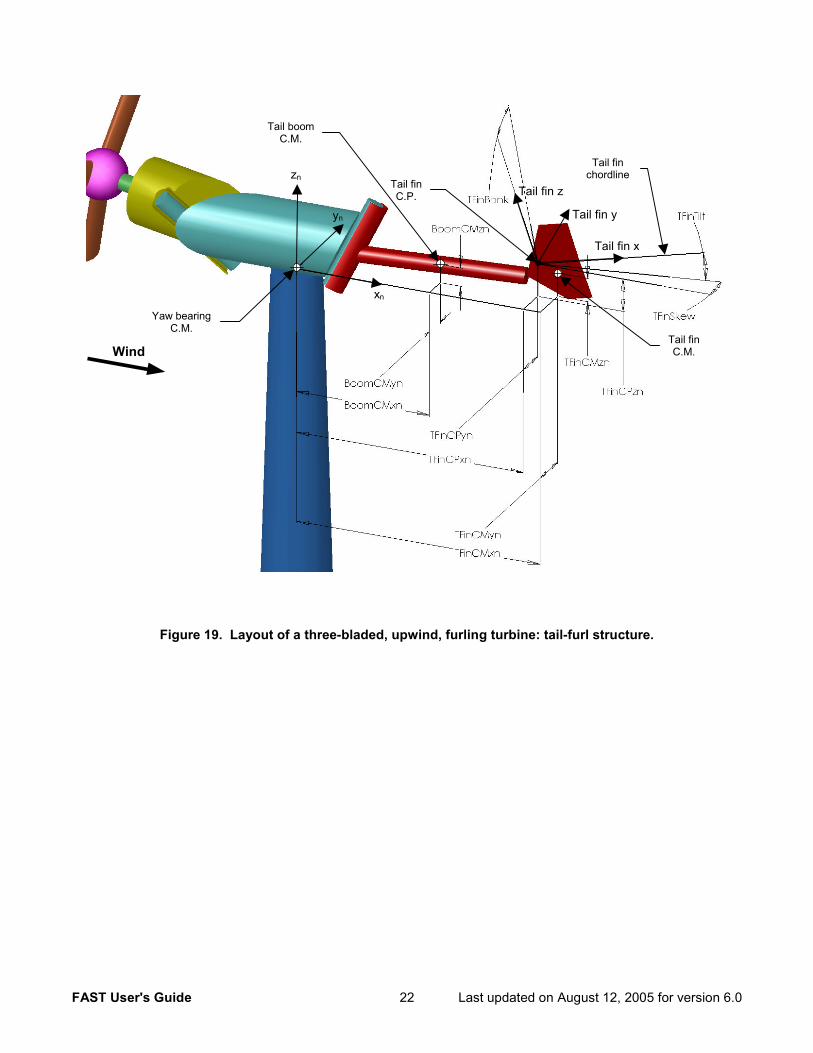
FAST User's Guide 22 Last updated on August 12, 2005 for version 6.0
Figure 19. Layout of a three-bladed, upwind, furling turbine: tail-furl structure.
zn
yn
xn
Tail fin chordline
Tail boom C.M.
Tail fin C.M.
Tail fin C.P.
Yaw bearing C.M.
Wind
Tail fin x
Tail fin z
Tail fin y
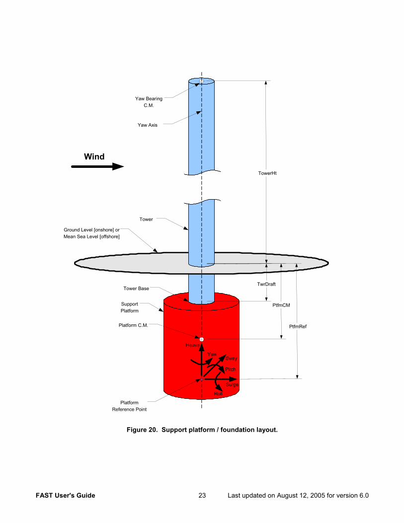
FAST User's Guide 23 Last updated on August 12, 2005 for version 6.0
Figure 20. Support platform / foundation layout.
Wind
TowerHt
TwrDraft
PtfmCM
Yaw BearingC.M.
Yaw Axis
PtfmRef
Ground Level [onshore] orMean Sea Level [offshore]
Platform C.M.
PlatformReference Point
SupportPlatform
Tower
Surge
Roll
Sway
Pitch
Yaw
Heave
Tower Base

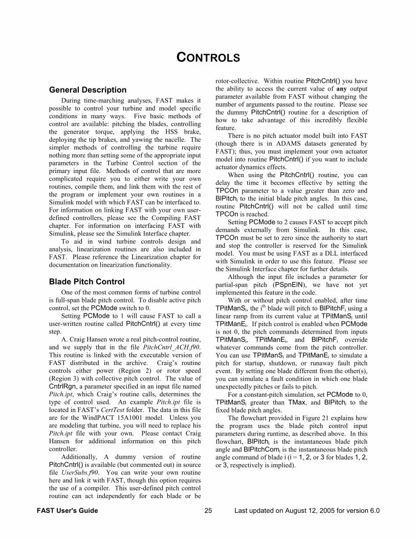
FAST User's Guide 25 Last updated on August 12, 2005 for version 6.0
CONTROLS
General Description During time-marching analyses, FAST makes it
possible to control your turbine and model specific conditions in many ways. Five basic methods of control are available: pitching the blades, controlling the generator torque, applying the HSS brake, deploying the tip brakes, and yawing the nacelle. The simpler methods of controlling the turbine require nothing more than setting some of the appropriate input parameters in the Turbine Control section of the primary input file. Methods of control that are more complicated require you to either write your own routines, compile them, and link them with the rest of the program or implement your own routines in a Simulink model with which FAST can be interfaced to. For information on linking FAST with your own user-defined controllers, please see the Compiling FAST chapter. For information on interfacing FAST with Simulink, please see the Simulink Interface chapter.
To aid in wind turbine controls design and analysis, linearization routines are also included in FAST. Please reference the Linearization chapter for documentation on linearization functionality.
Blade Pitch Control One of the most common forms of turbine control
is full-span blade pitch control. To disable active pitch control, set the PCMode switch to 0.
Setting PCMode to 1 will cause FAST to call a user-written routine called PitchCntrl() at every time step.
A. Craig Hansen wrote a real pitch-control routine, and we supply that in the file PitchCntrl_ACH.f90. This routine is linked with the executable version of FAST distributed in the archive. Craig’s routine controls either power (Region 2) or rotor speed (Region 3) with collective pitch control. The value of CntrlRgn, a parameter specified in an input file named Pitch.ipt, which Craig’s routine calls, determines the type of control used. An example Pitch.ipt file is located in FAST’s CertTest folder. The data in this file are for the WindPACT 15A1001 model. Unless you are modeling that turbine, you will need to replace his Pitch.ipt file with your own. Please contact Craig Hansen for additional information on this pitch controller.
Additionally, A dummy version of routine PitchCntrl() is available (but commented out) in source file UserSubs.f90. You can write your own routine here and link it with FAST, though this option requires the use of a compiler. This user-defined pitch control routine can act independently for each blade or be
rotor-collective. Within routine PitchCntrl() you have the ability to access the current value of any output parameter available from FAST without changing the number of arguments passed to the routine. Please see the dummy PitchCntrl() routine for a description of how to take advantage of this incredibly flexible feature.
There is no pitch actuator model built into FAST (though there is in ADAMS datasets generated by FAST); thus, you must implement your own actuator model into routine PitchCntrl() if you want to include actuator dynamics effects.
When using the PitchCntrl() routine, you can delay the time it becomes effective by setting the TPCOn parameter to a value greater than zero and BlPitchi to the initial blade pitch angles. In this case, routine PitchCntrl() will not be called until time TPCOn is reached.
Setting PCMode to 2 causes FAST to accept pitch demands externally from Simulink. In this case, TPCOn must be set to zero since the authority to start and stop the controller is reserved for the Simulink model. You must be using FAST as a DLL interfaced with Simulink in order to use this feature. Please see the Simulink Interface chapter for further details.
Although the input file includes a parameter for partial-span pitch (PSpnElN), we have not yet implemented this feature in the code.
With or without pitch control enabled, after time TPitManSi, the ith blade will pitch to BlPitchFi using a linear ramp from its current value at TPitManSi until TPitManEi. If pitch control is enabled when PCMode is not 0, the pitch commands determined from inputs TPitManSi, TPitManEi, and BlPitchFi override whatever commands come from the pitch controller. You can use TPitManSi and TPitManEi to simulate a pitch for startup, shutdown, or runaway fault pitch event. By setting one blade different from the other(s), you can simulate a fault condition in which one blade unexpectedly pitches or fails to pitch.
For a constant-pitch simulation, set PCMode to 0, TPitManSi greater than TMax, and BlPitchi to the fixed blade pitch angles.
The flowchart provided in Figure 21 explains how the program uses the blade pitch control input parameters during runtime, as described above. In this flowchart, BlPitchi is the instantaneous blade pitch angle and BlPitchComi is the instantaneous blade pitch angle command of blade i (i = 1, 2, or 3 for blades 1, 2, or 3, respectively is implied).
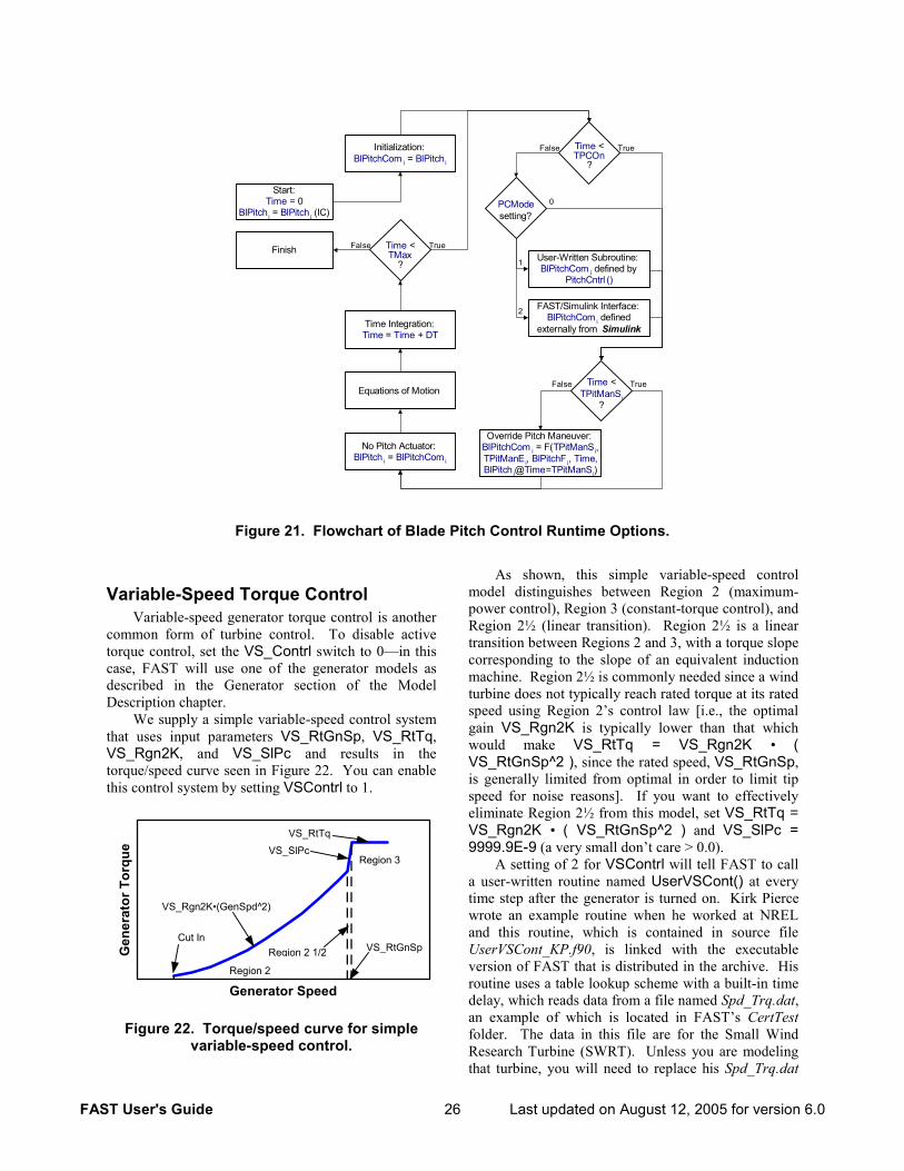
FAST User's Guide 26 Last updated on August 12, 2005 for version 6.0
Figure 21. Flowchart of Blade Pitch Control Runtime Options.
Variable-Speed Torque Control Variable-speed generator torque control is another
common form of turbine control. To disable active torque control, set the VS_Contrl switch to 0—in this case, FAST will use one of the generator models as described in the Generator section of the Model Description chapter.
We supply a simple variable-speed control system that uses input parameters VS_RtGnSp, VS_RtTq, VS_Rgn2K, and VS_SlPc and results in the torque/speed curve seen in Figure 22. You can enable this control system by setting VSContrl to 1.
Generator Speed
Gen
erat
or T
orqu
e
VS_RtGnSp
VS_Rgn2K•(GenSpd^2)
Region 2
Region 3
Cut InRegion 2 1/2
VS_RtTq
VS_SlPc
Figure 22. Torque/speed curve for simple
variable-speed control.
As shown, this simple variable-speed control model distinguishes between Region 2 (maximum-power control), Region 3 (constant-torque control), and Region 2½ (linear transition). Region 2½ is a linear transition between Regions 2 and 3, with a torque slope corresponding to the slope of an equivalent induction machine. Region 2½ is commonly needed since a wind turbine does not typically reach rated torque at its rated speed using Region 2’s control law [i.e., the optimal gain VS_Rgn2K is typically lower than that which would make VS_RtTq = VS_Rgn2K • ( VS_RtGnSp^2 ), since the rated speed, VS_RtGnSp, is generally limited from optimal in order to limit tip speed for noise reasons]. If you want to effectively eliminate Region 2½ from this model, set VS_RtTq = VS_Rgn2K • ( VS_RtGnSp^2 ) and VS_SlPc = 9999.9E-9 (a very small don’t care > 0.0).
A setting of 2 for VSContrl will tell FAST to call a user-written routine named UserVSCont() at every time step after the generator is turned on. Kirk Pierce wrote an example routine when he worked at NREL and this routine, which is contained in source file UserVSCont_KP.f90, is linked with the executable version of FAST that is distributed in the archive. His routine uses a table lookup scheme with a built-in time delay, which reads data from a file named Spd_Trq.dat, an example of which is located in FAST’s CertTest folder. The data in this file are for the Small Wind Research Turbine (SWRT). Unless you are modeling that turbine, you will need to replace his Spd_Trq.dat
FinishUser-Written Subroutine:BlPitchCom i defined by
PitchCntrl ()
FAST/Simulink Interface:BlPitchCom i defined
externally from Simulink
0
1
2
PCModesetting?
Time <TPCOn
?
False True
Time Integration:Time = Time + DT
Time <TMax
?
TrueFalse
Equations of MotionTime <
TPitManSi?
False True
Override Pitch Maneuver:BlPitchCom i = F(TPitManSi,TPitManEi, BlPitchFi, Time,BlPitchi@Time=TPitManSi)
No Pitch Actuator:BlPitch i = BlPitchComi
Initialization:BlPitchCom i = BlPitchi
Start:Time = 0
BlPitchi = BlPitchi (IC)
FAST User's Guide 27 Last updated on August 12, 2005 for version 6.0
file with your own. Please note that Kirk Pierce’s routine only works when GBRatio is set to 1.0.
Additionally, A dummy version of routine UserVSCont() is available (but commented out) in source file UserSubs.f90. You can write your own routine here and link it with FAST, though this option requires the use of a compiler. The routine that calls UserVSCont() passes the HSS speed and expects the electrical generator torque and electrical power to be returned. But within routine UserVSCont(), you have the ability to access the current value of any output parameter available from FAST without changing the number of arguments passed to the routine. Also, you have the option of switching the generator DOF on-or-off at runtime within UserVSCont() by overriding input GenDOF. Please see the supplied dummy routine in UserSubs.f90 for further details.
Setting VSContrl to 3 causes FAST to accept electrical generator torque and electrical power demands externally from Simulink. In this case, the authority to start and stop the generator is reserved for the Simulink model. Thus, GenTiStr and GenTiStp must be set to True, TimGenOn must be set to zero, and TimGenOf must be set greater than TMax. You must be using FAST as a DLL interfaced with Simulink in order to use this feature. Please see the Simulink Interface chapter for further details.
The flowchart provided in Figure 23 explains how the program uses the variable-speed torque control input parameters during runtime, as described above. In this flowchart, GenTq is the instantaneous electrical generator torque, GenPwr is the instantaneous electrical generator power, and GenSpeed is the instantaneous HSS (generator) speed. The additional logic presented in the flowchart explains how the program uses the generator model and HSS brake control input parameters during runtime.
HSS Brake Control By default, the HSS brake is disabled at the
beginning of a run. At time THSSBrDp, the brake will start to deploy. If you do not want the brake to deploy during a given run, set THSSBrDp to a value greater than TMax.
If you set HSSBrMode to 1, FAST will use a simple HSS brake model in which the brake torque will ramp linearly from zero at time THSSBrDp to full brake torque of HSSBrTqF over HSSBrDT seconds. The HSS brake is based on the Coulomb model of
sliding friction. Once full brake torque is reached, the magnitude of the torque is constant as long as the shaft speed is nonzero. When the speed is zero, the torque takes on any value to prevent motion of the shaft (the HSS can only move again if the external torque exceeds the full braking torque).
A user-defined HSS brake model is also available. Set HSSBRMode to 2 to tell FAST to call the user-written routine named UserHSSBr() at every time step after time THSSBrDp. A dummy version of routine UserHSSBr() is available in source file UserSubs.f90. You can write your own routine here and link it with FAST, though this option requires the use of a compiler. The routine that calls UserHSSBr() passes the HSS speed and time and expects the fraction of full braking torque to be returned (0.0 = off – no brake torque, 1.0 = full brake torque). As in the simple HSS brake model, the magnitude of the full breaking torque is specified in input HSSBrTqF. The fraction of full braking torque may continually vary, permitting you to continually switch the HSS brake on and off during the simulation. Input HSSBrDT is ignored when HSSBRMode is set to 2.
Within routine UserHSSBr(), you have the ability to access the current value of any output parameter available from FAST without changing the number of arguments passed to the routine. Also, you have the option of switching the generator DOF on-or-off at runtime within UserHSSBr() by overriding input GenDOF. Please see the supplied dummy routine in UserSubs.f90 for further details.
The flowchart provided in Figure 23 explains how the program uses the HSS brake control input parameters during runtime, as described above. In this flowchart, HSSBrFrac is the instantaneous fraction of full braking torque [limited to values between 0.0 and 1.0 (inclusive)] and GenSpeed is the instantaneous HSS (generator) speed. The additional logic presented in the flowchart explains how the program uses the variable-speed and generator model control input parameters during runtime.
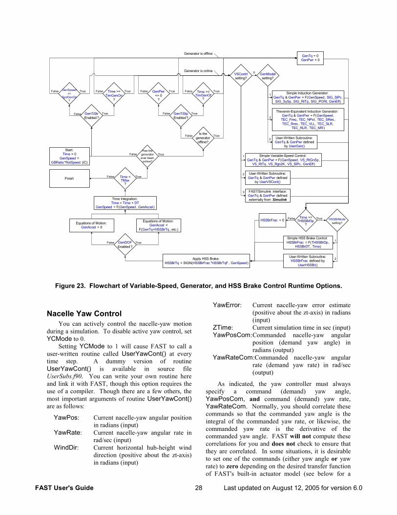
FAST User's Guide 28 Last updated on August 12, 2005 for version 6.0
Figure 23. Flowchart of Variable-Speed, Generator, and HSS Brake Control Runtime Options.
Nacelle Yaw Control You can actively control the nacelle-yaw motion
during a simulation. To disable active yaw control, set YCMode to 0.
Setting YCMode to 1 will cause FAST to call a user-written routine called UserYawCont() at every time step. A dummy version of routine UserYawCont() is available in source file UserSubs.f90. You can write your own routine here and link it with FAST, though this option requires the use of a compiler. Though there are a few others, the most important arguments of routine UserYawCont() are as follows:
YawPos: Current nacelle-yaw angular position in radians (input)
YawRate: Current nacelle-yaw angular rate in rad/sec (input)
WindDir: Current horizontal hub-height wind direction (positive about the zt-axis) in radians (input)
YawError: Current nacelle-yaw error estimate (positive about the zt-axis) in radians (input)
ZTime: Current simulation time in sec (input) YawPosCom: Commanded nacelle-yaw angular
position (demand yaw angle) in radians (output)
YawRateCom:Commanded nacelle-yaw angular rate (demand yaw rate) in rad/sec (output)
As indicated, the yaw controller must always specify a command (demand) yaw angle, YawPosCom, and command (demand) yaw rate, YawRateCom. Normally, you should correlate these commands so that the commanded yaw angle is the integral of the commanded yaw rate, or likewise, the commanded yaw rate is the derivative of the commanded yaw angle. FAST will not compute these correlations for you and does not check to ensure that they are correlated. In some situations, it is desirable to set one of the commands (either yaw angle or yaw rate) to zero depending on the desired transfer function of FAST's built-in actuator model (see below for a
User-Written Subroutine:GenTq & GenPwr defined
by UserVSCont()
Simple Variable-Speed Control:GenTq & GenPwr = F(GenSpeed , VS_RtGnSp ,
VS_RtTq , VS_Rgn2K, VS_SlPc, GenEff)
Simple Induction Generator:GenTq & GenPwr = F(GenSpeed, SIG_SlPc,SIG_SySp, SIG_RtTq, SIG_PORt, GenEff)
FAST/Simulink Interface:GenTq & GenPwr definedexternally from Simulink
Thevenin-Equivalent Induction Generator:GenTq & GenPwr = F(GenSpeed,
TEC_Freq , TEC_NPol , TEC_SRes,TEC_Rres , TEC_VLL , TEC_SLR,
TEC_RLR, TEC_MR)
GenTiStpEnabled?
GenTiStrEnabled?
GenSpeed>=
SpdGenOn?
Time >=TimGenOf
?
GenPwr<= 0
?
GenDOFEnabled?
TrueFalse TrueFalse
0
1
2
3
1
2
3
TrueTrue TrueTrueFalseFalse FalseFalse
GenTq = 0GenPwr = 0
TrueFalse
Time Integration:Time = Time + DT
GenSpeed = F(GenSpeed , GenAccel)
Time >=TimGenOn
?
Has thegeneratorever been
online?
False TrueStart:
Time = 0GenSpeed =
GBRatio*RotSpeed (IC)
Is thegeneratoroffline?
False True User-Written Subroutine:GenTq & GenPwr defined
by UserGen()
Generator is offline
Generator is onlineVSContrlsetting?
GenModelsetting?
Time <TMax
?
TrueFinish False
Equations of Motion:GenAccel = 0
Equations of Motion:GenAccel =
F(GenTq+HSSBrTq , etc.)
Simple HSS Brake Control:HSSBrFrac = F(THSSBrDp ,
HSSBrDT , Time)
HSSBrModesetting?
User-Written Subroutine:HSSBrFrac defined by
UserHSSBr()
1
2Apply HSS Brake:HSSBrTq = SIGN(HSSBrFrac *HSSBrTqF , GenSpeed)
HSSBrFrac = 0Time >=
THSSBrDp?
TrueFalse
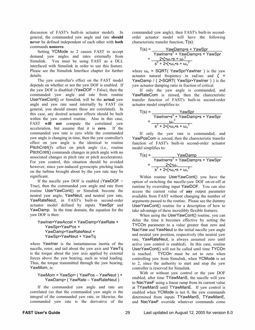
FAST User's Guide 29 Last updated on August 12, 2005 for version 6.0
discussion of FAST's built-in actuator model). In general, the commanded yaw angle and rate should never be defined independent of each other with both commands nonzero.
Setting YCMode to 2 causes FAST to accept demand yaw angles and rates externally from Simulink. You must be using FAST as a DLL interfaced with Simulink in order to use this feature. Please see the Simulink Interface chapter for further details.
The yaw controller's effect on the FAST model depends on whether or not the yaw DOF is enabled. If the yaw DOF is disabled (YawDOF = False), then the commanded yaw angle and rate from routine UserYawCont() or Simulink will be the actual yaw angle and yaw rate used internally by FAST (in general, you should ensure these are correlated). In this case, any desired actuator effects should be built within the yaw control routine. Also in this case, FAST will not compute the correlated yaw acceleration, but assume that it is zero. If the commanded yaw rate is zero while the commanded yaw angle is changing in time, then the yaw controller's effect on yaw angle is the identical to routine PitchCntrl()'s effect on pitch angle (i.e., routine PitchCntrl() commands changes in pitch angle with no associated changes in pitch rate or pitch acceleration). For yaw control, this situation should be avoided however, since yaw-induced gyroscopic pitching loads on the turbine brought about by the yaw rate may be significant.
If the nacelle yaw DOF is enabled (YawDOF = True), then the commanded yaw angle and rate from routine UserYawCont() or Simulink become the neutral yaw angle, YawNeut, and neutral yaw rate, YawRateNeut, in FAST's built-in second-order actuator model defined by inputs YawSpr and YawDamp. In the time domain, the equation for the yaw DOF is then:
YawIner•YawAccel + YawDamp•YawRate + YawSpr•YawPos = YawDamp•YawRateNeut + YawSpr•YawNeut + YawTq
where YawIner is the instantaneous inertia of the nacelle, rotor, and tail about the yaw axis and YawTq is the torque about the yaw axis applied by external forces above the yaw bearing, such as wind loading. Thus, the torque transmitted through the yaw bearing, YawMom, is:
YawMom = YawSpr• ( YawPos – YawNeut ) + YawDamp• ( YawRate – YawRateNeut )
If the commanded yaw angle and rate are correlated (so that the commanded yaw angle is the integral of the commanded yaw rate, or likewise, the commanded yaw rate is the derivative of the
commanded yaw angle), then FAST's built-in second-order actuator model will have the following characteristic transfer function, T(s):
T(s) = YawDamp•s + YawSpr YawIner•s2 + YawDamp•s + YawSpr = 2•ζ•ω n•s + ω n
2 s2 + 2•ζ•ωn•s + ωn
2
where ωn = SQRT( YawSpr/YawIner ) is the yaw actuator natural frequency in rad/sec and ζ = YawDamp / ( 2•SQRT( YawSpr•YawIner ) ) is the yaw actuator damping ratio in fraction of critical.
If only the yaw angle is commanded, and YawRateCom is zeroed, then the charecteristic transfer function of FAST's built-in second-order actuator model simplifies to:
T(s) = YawSpr YawIner•s2 + YawDamp•s + YawSpr = ω n
2 s2 + 2•ζ•ωn•s + ωn
2
If only the yaw rate is commanded, and YawPosCom is zeroed, then the charecteristic transfer function of FAST's built-in second-order actuator model simplifies to:
T(s) = YawDamp YawIner•s2 + YawDamp•s + YawSpr = 2•ζ•ω n s2 + 2•ζ•ωn•s + ωn
2
Within routine UserYawCont() you have the option of switching the nacelle-yaw DOF on-or-off at runtime by overriding input YawDOF. You can also access the current value of any output parameter available from FAST without changing the number of arguments passed to the routine. Please see the dummy UserYawCont() routine for a description of how to take advantage of these incredibly flexible features.
When using the UserYawCont() routine, you can delay the time it becomes effective by setting the TYCOn parameter to a value greater than zero and NacYaw and YawNeut to the initial nacelle yaw angle and neutral yaw position, respectively (the neutral yaw rate, YawRateNeut, is always assumed zero until active yaw control is enabled). In this case, routine UserYawCont() will not be called until time TYCOn is reached. TYCOn must be set to zero when controlling yaw from Simulink, when YCMode is set to 2, since the authority to start and stop the yaw controller is reserved for Simulink.
With or without yaw control or the yaw DOF enabled, after time TYawManS, the nacelle will yaw to NacYawF using a linear ramp from its current value at TYawManS until TYawManE. If yaw control is enabled when YCMode is not 0, the yaw commands determined from inputs TYawManS, TYawManE, and NacYawF override whatever commands come
FAST User's Guide 30 Last updated on August 12, 2005 for version 6.0
from the yaw controller. Also, the yaw commands determined from inputs TYawManS, TYawManE, and NacYawF pass through FAST’s built-in second-order actuator model if the yaw DOF is enabled when YawDOF is set to True. You can use TYawManS and TYawManE to simulate a yaw for startup, shutdown, or runaway yaw event.
For a fixed-yaw simulation, set YawDOF to False, YCMode to 0, TYawManS greater than TMax, and NacYaw to the fixed nacelle yaw angle.
You can also enable passive nacelle-yaw control during a simulation. Please see the Nacelle Yaw section in the Model Description chapter for information on passive yaw control options.
The flowchart provided in Figure 24 explains how the program uses the nacelle yaw control input parameters during runtime, as described above.
Figure 24. Flowchart of Nacelle Yaw Control Runtime Options.
Master Controllers and the Bladed-Style DLL Interface
In the Source folder of the FAST archive, we distribute a source file named BladedDLLInterface.f90. This source file contains example PitchCntrl(), UserHSSBr(), UserVSCont(), and UserYawCont() routines that may be used to interface FAST with a master controller implemented as a dynamic-link-library (DLL) in the style of Garrad Hassan's Bladed
wind turbine software package. All four routines call routine BladedDLLInterface(), which contains a call to the Bladed-style DLL that evaluates as DISCON(). See Figure 25 for a schematic. Routine BladedDLLInterface() USEs a MODULE named BladedDLLParameters(), which stores values of PARAMETER constants used in the interface. Routines BladedDLLInterface() and BladedDLLParameters() are also contained in source file BladedDLLInterface.f90.
Finish
User-Written Subroutine:YawPosCom & YawRateCom
defined by UserYawCont()
FAST/Simulink Interface:YawPosCom & YawRateCom
defined externally from Simulink
0
1
2
YCModesetting?
Time <TYCOn
?
False True
YawDOFEnabled?
TrueFalse
Time Integration:Time = Time + DT
YawPos = F(YawPos , YawRate )YawRate = F(YawRate , YawAccel )
Time <TMax
?
TrueFalse
Equations of Motion:YawAccel = 0
Equations of Motion:YawAccel = F(YawMom, etc.)
Yaw Actuator:YawNeut = YawPosCom
YawRateNeut = YawRateComYawMom = YawSpr*(YawPos-YawNeut )+ YawDamp*(YawRate -YawRateNeut )
Time <TYawManS
?
False True
Override Yaw Maneuver:YawPosCom & YawRateCom =
F(TYawManS, TYawManE, NacYawF,Time, YawPos@Time=TYawManS)
No Yaw Actuator:YawPos = YawPosCom
YawRate = YawRateCom
YawDOFEnabled?
TrueFalse
Initialization:YawPosCom = YawPos
YawRateCom = YawRate
Initialization:YawPosCom = YawNeut
YawRateCom = 0
Start:Time = 0
YawPos = NacYaw (IC)YawRate = 0
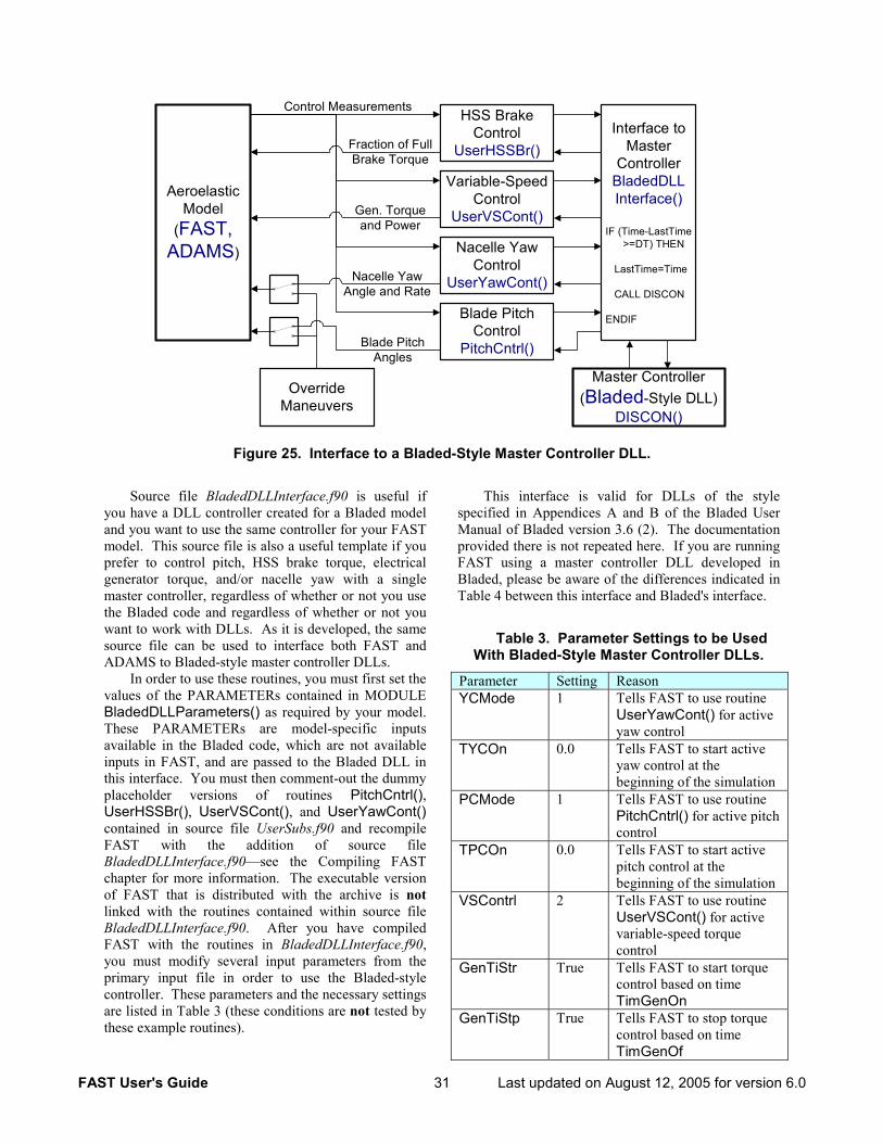
FAST User's Guide 31 Last updated on August 12, 2005 for version 6.0
Figure 25. Interface to a Bladed-Style Master Controller DLL.
Source file BladedDLLInterface.f90 is useful if you have a DLL controller created for a Bladed model and you want to use the same controller for your FAST model. This source file is also a useful template if you prefer to control pitch, HSS brake torque, electrical generator torque, and/or nacelle yaw with a single master controller, regardless of whether or not you use the Bladed code and regardless of whether or not you want to work with DLLs. As it is developed, the same source file can be used to interface both FAST and ADAMS to Bladed-style master controller DLLs.
In order to use these routines, you must first set the values of the PARAMETERs contained in MODULE BladedDLLParameters() as required by your model. These PARAMETERs are model-specific inputs available in the Bladed code, which are not available inputs in FAST, and are passed to the Bladed DLL in this interface. You must then comment-out the dummy placeholder versions of routines PitchCntrl(), UserHSSBr(), UserVSCont(), and UserYawCont() contained in source file UserSubs.f90 and recompile FAST with the addition of source file BladedDLLInterface.f90—see the Compiling FAST chapter for more information. The executable version of FAST that is distributed with the archive is not linked with the routines contained within source file BladedDLLInterface.f90. After you have compiled FAST with the routines in BladedDLLInterface.f90, you must modify several input parameters from the primary input file in order to use the Bladed-style controller. These parameters and the necessary settings are listed in Table 3 (these conditions are not tested by these example routines).
This interface is valid for DLLs of the style specified in Appendices A and B of the Bladed User Manual of Bladed version 3.6 (2). The documentation provided there is not repeated here. If you are running FAST using a master controller DLL developed in Bladed, please be aware of the differences indicated in Table 4 between this interface and Bladed's interface.
Table 3. Parameter Settings to be Used With Bladed-Style Master Controller DLLs.
Parameter Setting Reason YCMode 1 Tells FAST to use routine
UserYawCont() for active yaw control
TYCOn 0.0 Tells FAST to start active yaw control at the beginning of the simulation
PCMode 1 Tells FAST to use routine PitchCntrl() for active pitch control
TPCOn 0.0 Tells FAST to start active pitch control at the beginning of the simulation
VSContrl 2 Tells FAST to use routine UserVSCont() for active variable-speed torque control
GenTiStr True Tells FAST to start torque control based on time TimGenOn
GenTiStp True Tells FAST to stop torque control based on time TimGenOf
Blade PitchControl
PitchCntrl()
Nacelle YawControl
UserYawCont()
Variable-SpeedControl
UserVSCont()
AeroelasticModel
(FAST,ADAMS)
Blade PitchAngles
Nacelle YawAngle and Rate
Control Measurements
Gen. Torqueand Power
OverrideManeuvers
Interface toMaster
ControllerBladedDLLInterface()
IF (Time-LastTime >=DT) THEN
LastTime=Time
CALL DISCON
ENDIF
Master Controller(Bladed-Style DLL)
DISCON()
HSS BrakeControl
UserHSSBr()Fraction of FullBrake Torque
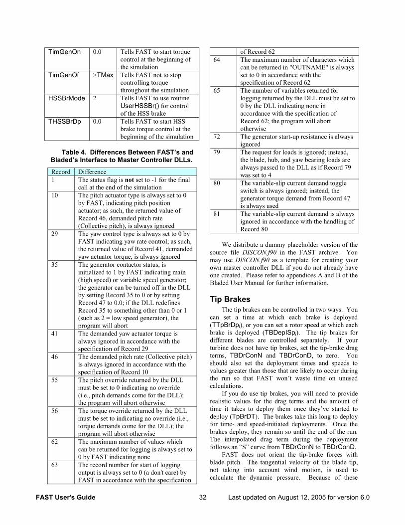
FAST User's Guide 32 Last updated on August 12, 2005 for version 6.0
TimGenOn 0.0 Tells FAST to start torque control at the beginning of the simulation
TimGenOf >TMax Tells FAST not to stop controlling torque throughout the simulation
HSSBrMode 2 Tells FAST to use routine UserHSSBr() for control of the HSS brake
THSSBrDp 0.0 Tells FAST to start HSS brake torque control at the beginning of the simulation
Table 4. Differences Between FAST’s and
Bladed’s Interface to Master Controller DLLs.
Record Difference 1 The status flag is not set to -1 for the final
call at the end of the simulation 10 The pitch actuator type is always set to 0
by FAST, indicating pitch position actuator; as such, the returned value of Record 46, demanded pitch rate (Collective pitch), is always ignored
29 The yaw control type is always set to 0 by FAST indicating yaw rate control; as such, the returned value of Record 41, demanded yaw actuator torque, is always ignored
35 The generator contactor status, is initialized to 1 by FAST indicating main (high speed) or variable speed generator; the generator can be turned off in the DLL by setting Record 35 to 0 or by setting Record 47 to 0.0; if the DLL redefines Record 35 to something other than 0 or 1 (such as 2 = low speed generator), the program will abort
41 The demanded yaw actuator torque is always ignored in accordance with the specification of Record 29
46 The demanded pitch rate (Collective pitch) is always ignored in accordance with the specification of Record 10
55 The pitch override returned by the DLL must be set to 0 indicating no override (i.e., pitch demands come for the DLL); the program will abort otherwise
56 The torque override returned by the DLL must be set to indicating no override (i.e., torque demands come for the DLL); the program will abort otherwise
62 The maximum number of values which can be returned for logging is always set to 0 by FAST indicating none
63 The record number for start of logging output is always set to 0 (a don't care) by FAST in accordance with the specification
of Record 62 64 The maximum number of characters which
can be returned in "OUTNAME" is always set to 0 in accordance with the specification of Record 62
65 The number of variables returned for logging returned by the DLL must be set to 0 by the DLL indicating none in accordance with the specification of Record 62; the program will abort otherwise
72 The generator start-up resistance is always ignored
79 The request for loads is ignored; instead, the blade, hub, and yaw bearing loads are always passed to the DLL as if Record 79 was set to 4
80 The variable-slip current demand toggle switch is always ignored; instead, the generator torque demand from Record 47 is always used
81 The variable-slip current demand is always ignored in accordance with the handling of Record 80
We distribute a dummy placeholder version of the
source file DISCON.f90 in the FAST archive. You may use DISCON.f90 as a template for creating your own master controller DLL if you do not already have one created. Please refer to appendices A and B of the Bladed User Manual for further information.
Tip Brakes The tip brakes can be controlled in two ways. You
can set a time at which each brake is deployed (TTpBrDpi), or you can set a rotor speed at which each brake is deployed (TBDepISpi). The tip brakes for different blades are controlled separately. If your turbine does not have tip brakes, set the tip-brake drag terms, TBDrConN and TBDrConD, to zero. You should also set the deployment times and speeds to values greater than those that are likely to occur during the run so that FAST won’t waste time on unused calculations.
If you do use tip brakes, you will need to provide realistic values for the drag terms and the amount of time it takes to deploy them once they’ve started to deploy (TpBrDT). The brakes take this long to deploy for time- and speed-initiated deployments. Once the brakes deploy, they remain so until the end of the run. The interpolated drag term during the deployment follows an “S” curve from TBDrConN to TBDrConD.
FAST does not orient the tip-brake forces with blade pitch. The tangential velocity of the blade tip, not taking into account wind motion, is used to calculate the dynamic pressure. Because of these
FAST User's Guide 33 Last updated on August 12, 2005 for version 6.0
approximations, you should adjust TBDrConD so that the rotor decelerates as expected.
Simulating Special Events There are many special events that can be modeled
with FAST. Although we will illustrate many of them in this section, we cannot document all of them. We hope that these examples will be sufficient so that you can figure out how to model other cases.
Turbine Startup There are several ways to start a turbine. One
common way is to pitch the blades from feather to the run position and let the wind accelerate the rotor until a certain speed is reached. To model this case, set PCMode to 0, GenTiStr to False, and SpdGenOn to an appropriate value. For each blade, set TPitManS to the time you want to start the maneuver, TPitManE to the end time for the maneuver, BlPitch to the feather position, and BlPitchF to the run position.
You can also start a stall-regulated turbine by motoring. To perform a motor start, set PCMode to 0, GenTiStr to True, and TimGenOn to an appropriate value. You should also use either variable-speed control or the Thevenin-equivalent-induction-generator model. Do not use the simple-induction-generator model, because it does not have a realistic startup torque.
Normal Pitch-to-Feather Shutdown To simulate this case, you’ll need to set the pitch
maneuver start and stop times (TPitManS and TPitManE) and the initial and final pitch settings (BlPitch and BlPitchF). Set TiGenOn to zero and, if you want to use the generator as a brake, set GenTiStp to False. This will disengage the generator when the turbine slows enough to drop the power to zero.
Shutdown Where One Blade Fails to Feather This case is the same as the previous example, but
either set the times (TPitManS and TPitManE) for one blade to values greater than TMax or set the final pitch value, BlPitchF, to the initial pitch value (BlPitch) or some other value that is different from the other blade(s).
One Blade Feathers Accidentally This case is the same as the previous example, but
either set the times (TPitManS and TPitManE) for the non-feathering blade(s) to values greater than TMax, or set the final pitch value(s), BlPitchF, to the initial pitch value(s) (BlPitch).
HSS Brake Shutdown after Loss of Grid To model an emergency shutdown where the HSS
brake stops the rotor, set GenTiStp to True and TimGenOf to the time you want the grid to fail. When using the simple built-in HSS brake model
(HSSBrMode = 1), set THSSBrDp to a short time after TimGenOf and HSSBrDt to the amount of time it takes to fully apply the brake (the brake torque will ramp from zero to full in a linear fashion). When using a user-defined HSS brake model (HSSBrMode = 2), you may specify a nonlinear ramp. Input HSSBrTqF specifies the maximum full brake torque in both cases.
HSS Brake Shutdown with Generator Brake FAST can model a shutdown in which the
generator acts as a dynamic brake until the rotor slows enough that the HSS brake can stop the rotor, but for now you must write the logic yourself by supplying a UserGen() routine and linking it with the rest of the code. We hope to find an easier way by adding a few input parameters.
Normal Tip Brake Shutdown To model a normal shutdown, in which the tip
brakes decelerate the rotor, set TTpBrDp to appropriate values for each blade. As with the pitch-to-feather shutdown, set GenTiStp to False so that the generator will disengage when power drops to zero.
Tip Brake Shutdown after Loss of Grid This case is similar to the previous case, but you’ll
use the TBDepISp array to make FAST use rotor speed to deploy the tip brakes. You can also model the special case in which one brake deploys at a higher speed than the other(s) or not at all by setting its deployment initiation speed to a higher speed.
Accidental Deployment of a Tip Brake You can easily model the accidental deployment
of a tip brake. For one blade, set TTpBrDp to a value less than TMax. For the other blade(s), set TTpBrDp to value(s) greater than TMax. For all blades, set TBDepISp to large numbers so that the brakes will never deploy because of rotor speed. You will also need to set TBDrConN, TBDrConD, and TpBrDT to appropriate values.
Idling Turbine You can simulate an idling turbine by enabling the
generator DOF (GenDOF) and setting GenTiStr to True and TimGenOn to a value greater than TMax to ensure that the generator never goes online. You will also want to initialize the rotor speed (RotSpeed) to a small or zero value, set the generator inertia (GenIner) to a non-zero value, and set the gearbox efficiency (GboxEff) to a value less than 100%. The torque passing through the non-perfect gearbox to the generator-rotor inertia will tend to resist acceleration of the turbine rotor. You can also add some speed-independent drag to the drivetrain by applying a light brake load. To do so, tell the brake to always be on by setting THSSBrDp and HSSBrDt to 0, and then set the brake torque (HSSBrTqF) to a small value.
FAST User's Guide 34 Last updated on August 12, 2005 for version 6.0
Parked Turbine One of the standard IEC test cases is to model the
turbine in high winds when the turbine is parked. If your turbine uses full-span pitch, set the values of BlPitch and BlPitchF to the feathered setting. Also set TpitManS and TpitManE to 0 so the blades are feathered during the entire simulation.
If you park your turbine by applying a HSS brake, you can model this condition by disabling the generator DOF (GenDOF) with RotSpeed set to zero and enabling the drivetrain DOF (DrTrDOF) to allow the
drivetrain to ring. Another possibility is to enable GenDOF, but set GenTiStr and TimGenOn so the generator never starts. Set THSSBrDp and HSSBrDT to zero so the HSS brake is always on. You will need to set the HSSBrTqF to a realistic value.
For potential failure modes, you can model the case in which the brake torque is insufficient to hold the turbine. The generator DOF must be enabled for this case. You can examine another potential failure by setting one of the blades so that it pitches to a non-feathered value at some time during the run.
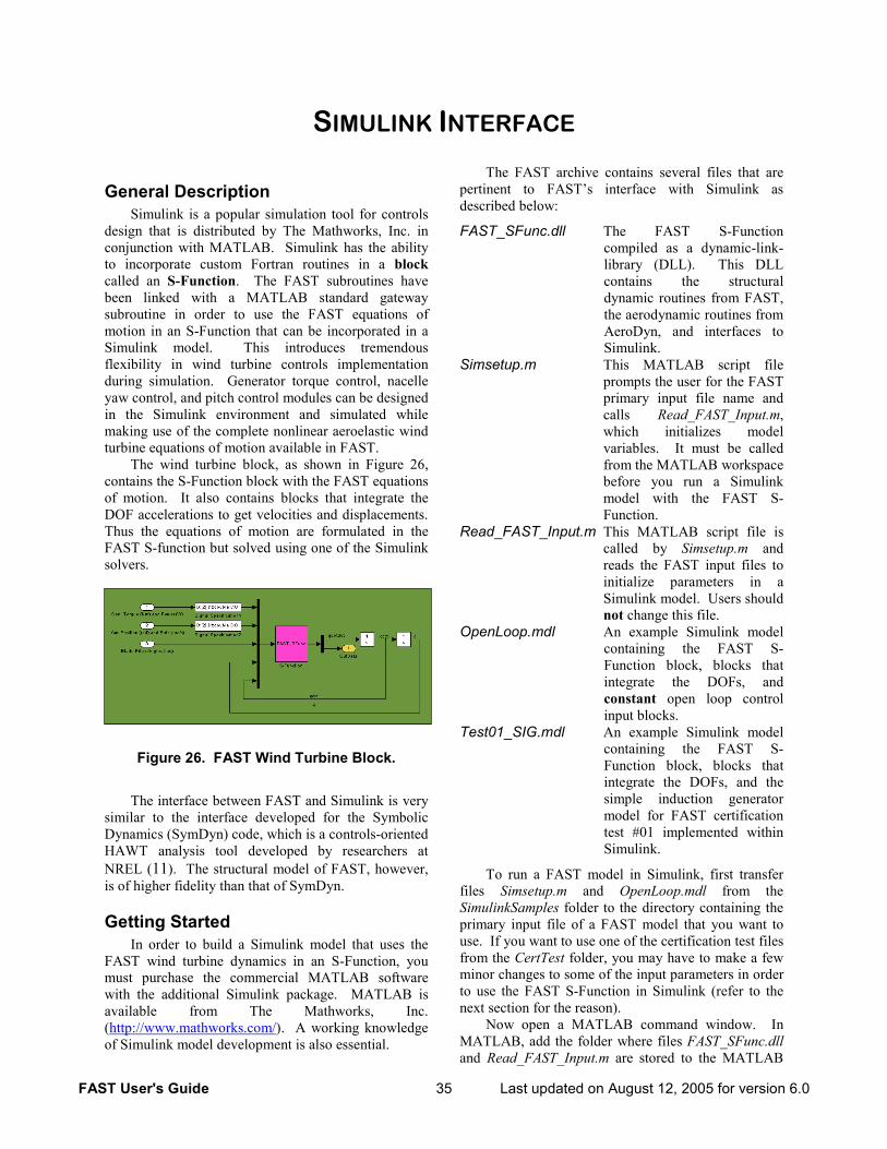
FAST User's Guide 35 Last updated on August 12, 2005 for version 6.0
SIMULINK INTERFACE
General Description Simulink is a popular simulation tool for controls
design that is distributed by The Mathworks, Inc. in conjunction with MATLAB. Simulink has the ability to incorporate custom Fortran routines in a block called an S-Function. The FAST subroutines have been linked with a MATLAB standard gateway subroutine in order to use the FAST equations of motion in an S-Function that can be incorporated in a Simulink model. This introduces tremendous flexibility in wind turbine controls implementation during simulation. Generator torque control, nacelle yaw control, and pitch control modules can be designed in the Simulink environment and simulated while making use of the complete nonlinear aeroelastic wind turbine equations of motion available in FAST.
The wind turbine block, as shown in Figure 26, contains the S-Function block with the FAST equations of motion. It also contains blocks that integrate the DOF accelerations to get velocities and displacements. Thus the equations of motion are formulated in the FAST S-function but solved using one of the Simulink solvers.
Figure 26. FAST Wind Turbine Block.
The interface between FAST and Simulink is very similar to the interface developed for the Symbolic Dynamics (SymDyn) code, which is a controls-oriented HAWT analysis tool developed by researchers at NREL (11). The structural model of FAST, however, is of higher fidelity than that of SymDyn.
Getting Started In order to build a Simulink model that uses the
FAST wind turbine dynamics in an S-Function, you must purchase the commercial MATLAB software with the additional Simulink package. MATLAB is available from The Mathworks, Inc. (http://www.mathworks.com/). A working knowledge of Simulink model development is also essential.
The FAST archive contains several files that are pertinent to FAST’s interface with Simulink as described below:
FAST_SFunc.dll The FAST S-Function compiled as a dynamic-link-library (DLL). This DLL contains the structural dynamic routines from FAST, the aerodynamic routines from AeroDyn, and interfaces to Simulink.
Simsetup.m This MATLAB script file prompts the user for the FAST primary input file name and calls Read_FAST_Input.m, which initializes model variables. It must be called from the MATLAB workspace before you run a Simulink model with the FAST S-Function.
Read_FAST_Input.m This MATLAB script file is called by Simsetup.m and reads the FAST input files to initialize parameters in a Simulink model. Users should not change this file.
OpenLoop.mdl An example Simulink model containing the FAST S-Function block, blocks that integrate the DOFs, and constant open loop control input blocks.
Test01_SIG.mdl An example Simulink model containing the FAST S-Function block, blocks that integrate the DOFs, and the simple induction generator model for FAST certification test #01 implemented within Simulink.
To run a FAST model in Simulink, first transfer files Simsetup.m and OpenLoop.mdl from the SimulinkSamples folder to the directory containing the primary input file of a FAST model that you want to use. If you want to use one of the certification test files from the CertTest folder, you may have to make a few minor changes to some of the input parameters in order to use the FAST S-Function in Simulink (refer to the next section for the reason).
Now open a MATLAB command window. In MATLAB, add the folder where files FAST_SFunc.dll and Read_FAST_Input.m are stored to the MATLAB
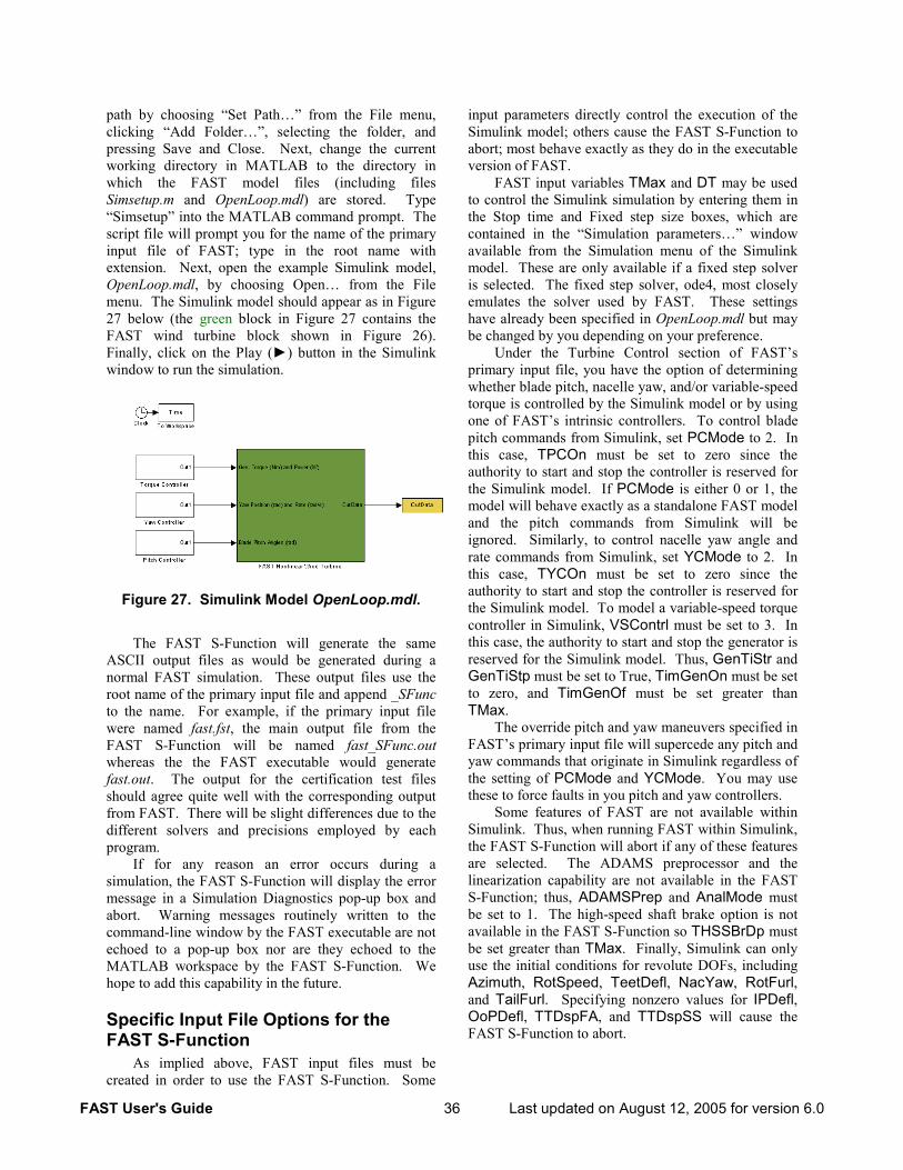
FAST User's Guide 36 Last updated on August 12, 2005 for version 6.0
path by choosing “Set Path…” from the File menu, clicking “Add Folder…”, selecting the folder, and pressing Save and Close. Next, change the current working directory in MATLAB to the directory in which the FAST model files (including files Simsetup.m and OpenLoop.mdl) are stored. Type “Simsetup” into the MATLAB command prompt. The script file will prompt you for the name of the primary input file of FAST; type in the root name with extension. Next, open the example Simulink model, OpenLoop.mdl, by choosing Open… from the File menu. The Simulink model should appear as in Figure 27 below (the green block in Figure 27 contains the FAST wind turbine block shown in Figure 26). Finally, click on the Play () button in the Simulink window to run the simulation.
Figure 27. Simulink Model OpenLoop.mdl.
The FAST S-Function will generate the same ASCII output files as would be generated during a normal FAST simulation. These output files use the root name of the primary input file and append _SFunc to the name. For example, if the primary input file were named fast.fst, the main output file from the FAST S-Function will be named fast_SFunc.out whereas the the FAST executable would generate fast.out. The output for the certification test files should agree quite well with the corresponding output from FAST. There will be slight differences due to the different solvers and precisions employed by each program.
If for any reason an error occurs during a simulation, the FAST S-Function will display the error message in a Simulation Diagnostics pop-up box and abort. Warning messages routinely written to the command-line window by the FAST executable are not echoed to a pop-up box nor are they echoed to the MATLAB workspace by the FAST S-Function. We hope to add this capability in the future.
Specific Input File Options for the FAST S-Function
As implied above, FAST input files must be created in order to use the FAST S-Function. Some
input parameters directly control the execution of the Simulink model; others cause the FAST S-Function to abort; most behave exactly as they do in the executable version of FAST.
FAST input variables TMax and DT may be used to control the Simulink simulation by entering them in the Stop time and Fixed step size boxes, which are contained in the “Simulation parameters…” window available from the Simulation menu of the Simulink model. These are only available if a fixed step solver is selected. The fixed step solver, ode4, most closely emulates the solver used by FAST. These settings have already been specified in OpenLoop.mdl but may be changed by you depending on your preference.
Under the Turbine Control section of FAST’s primary input file, you have the option of determining whether blade pitch, nacelle yaw, and/or variable-speed torque is controlled by the Simulink model or by using one of FAST’s intrinsic controllers. To control blade pitch commands from Simulink, set PCMode to 2. In this case, TPCOn must be set to zero since the authority to start and stop the controller is reserved for the Simulink model. If PCMode is either 0 or 1, the model will behave exactly as a standalone FAST model and the pitch commands from Simulink will be ignored. Similarly, to control nacelle yaw angle and rate commands from Simulink, set YCMode to 2. In this case, TYCOn must be set to zero since the authority to start and stop the controller is reserved for the Simulink model. To model a variable-speed torque controller in Simulink, VSContrl must be set to 3. In this case, the authority to start and stop the generator is reserved for the Simulink model. Thus, GenTiStr and GenTiStp must be set to True, TimGenOn must be set to zero, and TimGenOf must be set greater than TMax.
The override pitch and yaw maneuvers specified in FAST’s primary input file will supercede any pitch and yaw commands that originate in Simulink regardless of the setting of PCMode and YCMode. You may use these to force faults in you pitch and yaw controllers.
Some features of FAST are not available within Simulink. Thus, when running FAST within Simulink, the FAST S-Function will abort if any of these features are selected. The ADAMS preprocessor and the linearization capability are not available in the FAST S-Function; thus, ADAMSPrep and AnalMode must be set to 1. The high-speed shaft brake option is not available in the FAST S-Function so THSSBrDp must be set greater than TMax. Finally, Simulink can only use the initial conditions for revolute DOFs, including Azimuth, RotSpeed, TeetDefl, NacYaw, RotFurl, and TailFurl. Specifying nonzero values for IPDefl, OoPDefl, TTDspFA, and TTDspSS will cause the FAST S-Function to abort.
FAST User's Guide 37 Last updated on August 12, 2005 for version 6.0
Customizing the Simulink Model This section provides a few more details on the
FAST interface to Simulink. This should provide you with enough guidance so that you can modify the example Simulink models to include your own torque, yaw, and/or pitch controllers.
The wind turbine block requires three inputs and has one output as shown in Figure 26 and Figure 27. Electrical generator torque and electric power demands must be supplied in the first input, nacelle yaw position and rate demands must be supplied in the second input, and blade pitch demand angles for all blades must be supplied in the third input. Data must be provided for all inputs in order for the Simulink model to run. For instance, if you want to use the FAST simple induction generator model (by setting VSContrl to 0 and GenModel to 1) rather than developing a torque controller in your Simulink model, you may use Constant blocks to supply dummy electrical generator torque and electrical power demands to the FAST wind turbine block—these will not be used by the wind turbine block, but they must be present. This is demonstrated in OpenLoop.mdl. Similarly, values must be supplied for the yaw position and rate, and the blade pitch angles. The blade pitch angles are stored in a vector sized according to the number of blades.
In addition to the data available in the primary output file generated by the S-Function, the wind turbine block will also output a variable array named OutData that contains the output data selected in the FAST input file through input OutList. OutData contains output data at every model time step (whereas the primary output file uses the value of DecFact) and is available in the Simulink environment at runtime for feeding back control measurements. Thus, the control measurement channels your Simulink controller needs must be specified in OutList. OutData will also be available in the MATLAB workspace for postprocessing.
The output data names listed in OutList are also available in MATLAB and Simulink workspaces in a variable cell array named, appropriately, OutList. This variable is created by the Read_FAST_Input.m script
file. You can access specific channels from the OutData array by using the OutList cell array. For example, to obtain the rotor speed (assuming rotor speed was specified in OutList) at the 3rd time step (3rd row) in the MATLAB workspace, type “OutData(3,strmatch(‘RotSpeed’,OutList))” in the MATLAB command prompt. Using this technique, you don’t need to remember the specific order you listed the output channel names in OutList.
You can modify the Simsetup.m script file to initialize variables for any additions you make to the Simulink model for torque, yaw, and pitch control. If you modify Simsetup.m, remember to use “clear all” or “clear functions” to clear the MATLAB memory before repeating a simulation. As provided, “clear all” is the first command in Simsetup.m. The character array named input_fast, which is defined in Simsetup.m, must contain the name of the primary input file. Also, the script that reads the FAST input file for model initialization, Read_FAST_Input.m, must be called before running a simulation and after input_fast has been defined. Other than these requirements, you are free to perform any controller design or initialization steps in Simsetup.m or your own script before performing a simulation in Simulink.
As an example of a Simulink model more advanced than OpenLoop.mdl, we distribute a Simulink model named Test01_SIG.mdl in the FAST archive. In this example, the simple induction generator (available when VSContrl is set to 0 and GenModel is set to 1) is implemented in Simulink rather than FAST for certification test #01 (by setting VSContrl to 2). To run this example, follow the directions in the comments at the end of Simsetup.m. The output should be very similar to that of certification test #01 run with the FAST executable. There will be slight differences due to the different solvers and precisions employed by each program.

FAST User's Guide 39 Last updated on August 12, 2005 for version 6.0
LINEARIZATION
General Description FAST has the capability of extracting linearized
representations of the complete nonlinear aeroelastic wind turbine modeled in the code. This analysis capability is useful for developing state matrices of a wind turbine “plant” to aid in controls design and analysis. It is also useful for determining the full system modes of an operating or stationary HAWT through the use of a simple eigenanalysis. A FAST linearization analysis is invoked by setting input parameter AnalMode in the primary input file to 2.
The linearization routines follow a procedure similar to that used by the Symbolic Dynamics (SymDyn) code, which is a controls-oriented HAWT analysis tool developed by researchers at NREL (11). The structural model of FAST, however, is of higher fidelity than that of SymDyn.
The linearization process consists of two steps: (1) computing a periodic steady state operating point condition for the DOFs and (2) numerically linearizing the FAST model about this operating point to form periodic state matrices. The output state matrices can then be azimuth-averaged for nonperiodic, or time-invariant controls development.
Periodic Steady State Solution The first step in the linearization process is
determining an operating point to linearize the model about. An operating point is a set of values of the system DOF displacements, DOF velocities, DOF accelerations, control inputs, and wind inputs that characterize a steady condition of the wind turbine. For a wind turbine operating in steady winds, this operating point is periodic—that is, the operating point values depend on the rotor azimuth orientation. This periodicity is driven by aerodynamic loads, which depend on the rotor azimuth position in the presence of prescribed shaft tilt, wind shear, yaw error, or tower shadow. Gravitational loads also drive the periodic behavior when there is a prescribed shaft tilt or appreciable deflection of the tower due to thrust loading. It is important to determine an accurate operating point because the linearized model is only accurate for values of the DOFs and inputs that are close to the operating point values.
To compute a steady state solution, the program inputs must necessarily produce a time invariant model (other than azimuth dependence). To insure this time invariant condition, FAST performs a number of checks on some of the input parameters before running a linearization analysis. FAST will abort without computing the linearized state matrices if any of the
following conditions are not met. First, active yaw and pitch control must be disabled by setting YCMode and PCMode to 0. FAST can’t be linearized during a startup or shutdown event, thus GenTiStr and GenTiStp must both be set True, TimGenOn must be set to 0.0, and TimGenOf must be set greater than TMax during a linearization analysis. Inputs THSSBrDp, TiDynBrk, TTpBrDpi, TYawManS, and TPitManSi must also be set greater than TMax, and TBDepISpi must be set much greater than RotSpeed. In AeroDyn, dynamic stall and dynamic inflow must be disabled if CompAero is True; thus StallMod should be set to “STEADY” and InfModel to “EQUIIL”ibrium. Also, you must use a hub-height wind data file (input WindFile) that does not vary with time. At least one DOF must be enabled during a linearization analysis because it is useless to have a “plant” model with zero states. Finally, CompNoise must be disabled during a linearization analysis.
Inputs CalcStdy, TrimCase, DispTol, and VelTol, which are available in the linearization control-input-file of FAST (identified by parameter LinFile in FAST’s primary input file), are the parameters used to manage the steady state solution computation in FAST.
Input parameter CalcStdy is a flag used to indicate whether a periodic steady state solution is computed before linearizing the model. To disable the steady state solution computation, set CalcStdy to False. In this case, the operating point is prescribed by the values of the initial conditions specified in FAST’s primary input file. That is, when CalcStdy is False, the operating point is set to the condition in which all displacements, velocities, and accelerations are zero, except those specified with nonzero initial conditions (for instance, the azimuth DOF will increment at a constant rate if and when the rotor is spinning).
Setting CalcStdy to True causes FAST to compute a steady state solution before linearizing the model. During a steady state solution computation, FAST integrates the nonlinear equations of motion in time until the solution “converges”. “Convergence” is determined as follows. At each iteration, or one period of revolution of the rotor, a 2-norm of the differences between conditions at the beginning and end of the iteration is computed. A 2-norm is computed for both the angular displacement vector differences and angular velocity vector differences. Input parameters DispTol and VelTol are used as convergence tolerances for the displacement 2-norm and velocity 2-norm, respectively. The smaller the values of DispTol and VelTol, the tighter the tolerances. Once both of the computed 2-norms become smaller than or equal to the input convergence tolerances, the solution is considered to have “converged”. If the solution has not
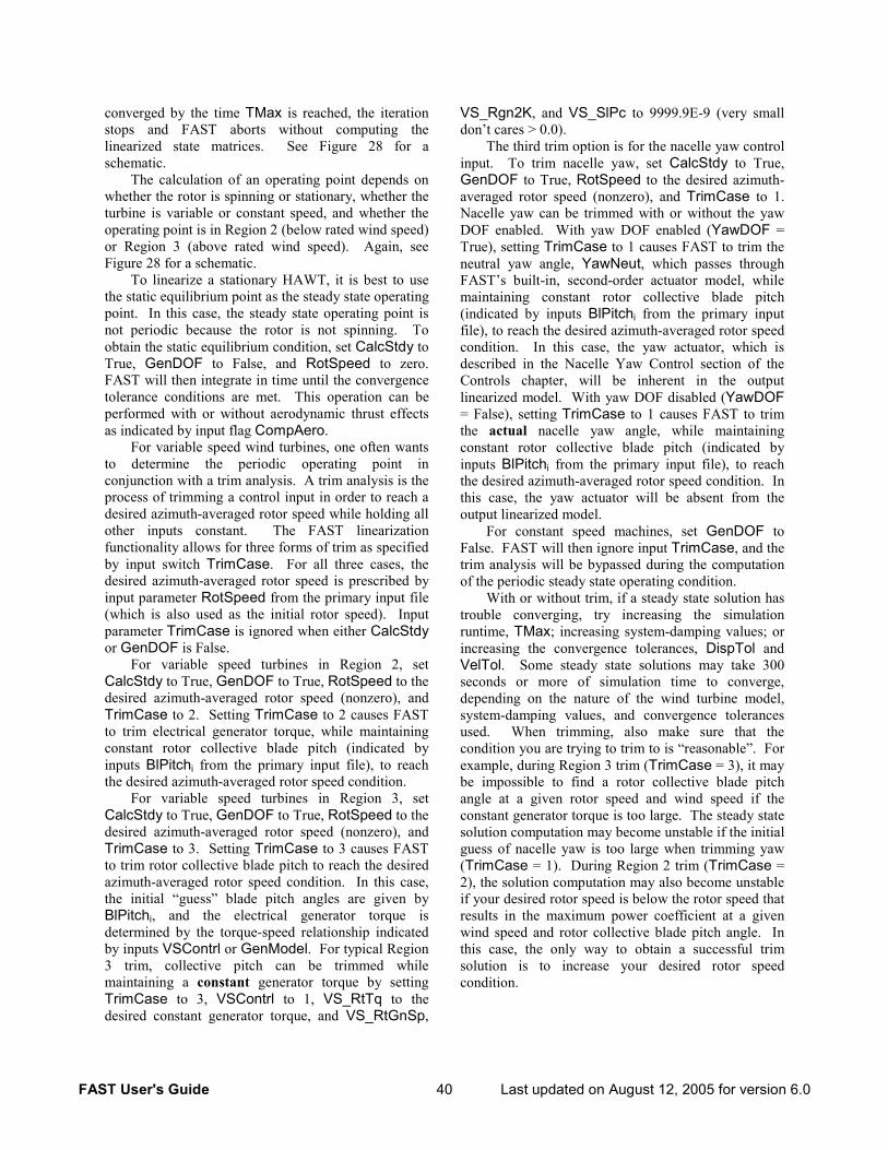
FAST User's Guide 40 Last updated on August 12, 2005 for version 6.0
converged by the time TMax is reached, the iteration stops and FAST aborts without computing the linearized state matrices. See Figure 28 for a schematic.
The calculation of an operating point depends on whether the rotor is spinning or stationary, whether the turbine is variable or constant speed, and whether the operating point is in Region 2 (below rated wind speed) or Region 3 (above rated wind speed). Again, see Figure 28 for a schematic.
To linearize a stationary HAWT, it is best to use the static equilibrium point as the steady state operating point. In this case, the steady state operating point is not periodic because the rotor is not spinning. To obtain the static equilibrium condition, set CalcStdy to True, GenDOF to False, and RotSpeed to zero. FAST will then integrate in time until the convergence tolerance conditions are met. This operation can be performed with or without aerodynamic thrust effects as indicated by input flag CompAero.
For variable speed wind turbines, one often wants to determine the periodic operating point in conjunction with a trim analysis. A trim analysis is the process of trimming a control input in order to reach a desired azimuth-averaged rotor speed while holding all other inputs constant. The FAST linearization functionality allows for three forms of trim as specified by input switch TrimCase. For all three cases, the desired azimuth-averaged rotor speed is prescribed by input parameter RotSpeed from the primary input file (which is also used as the initial rotor speed). Input parameter TrimCase is ignored when either CalcStdy or GenDOF is False.
For variable speed turbines in Region 2, set CalcStdy to True, GenDOF to True, RotSpeed to the desired azimuth-averaged rotor speed (nonzero), and TrimCase to 2. Setting TrimCase to 2 causes FAST to trim electrical generator torque, while maintaining constant rotor collective blade pitch (indicated by inputs BlPitchi from the primary input file), to reach the desired azimuth-averaged rotor speed condition.
For variable speed turbines in Region 3, set CalcStdy to True, GenDOF to True, RotSpeed to the desired azimuth-averaged rotor speed (nonzero), and TrimCase to 3. Setting TrimCase to 3 causes FAST to trim rotor collective blade pitch to reach the desired azimuth-averaged rotor speed condition. In this case, the initial “guess” blade pitch angles are given by BlPitchi, and the electrical generator torque is determined by the torque-speed relationship indicated by inputs VSContrl or GenModel. For typical Region 3 trim, collective pitch can be trimmed while maintaining a constant generator torque by setting TrimCase to 3, VSContrl to 1, VS_RtTq to the desired constant generator torque, and VS_RtGnSp,
VS_Rgn2K, and VS_SlPc to 9999.9E-9 (very small don’t cares > 0.0).
The third trim option is for the nacelle yaw control input. To trim nacelle yaw, set CalcStdy to True, GenDOF to True, RotSpeed to the desired azimuth-averaged rotor speed (nonzero), and TrimCase to 1. Nacelle yaw can be trimmed with or without the yaw DOF enabled. With yaw DOF enabled (YawDOF = True), setting TrimCase to 1 causes FAST to trim the neutral yaw angle, YawNeut, which passes through FAST’s built-in, second-order actuator model, while maintaining constant rotor collective blade pitch (indicated by inputs BlPitchi from the primary input file), to reach the desired azimuth-averaged rotor speed condition. In this case, the yaw actuator, which is described in the Nacelle Yaw Control section of the Controls chapter, will be inherent in the output linearized model. With yaw DOF disabled (YawDOF = False), setting TrimCase to 1 causes FAST to trim the actual nacelle yaw angle, while maintaining constant rotor collective blade pitch (indicated by inputs BlPitchi from the primary input file), to reach the desired azimuth-averaged rotor speed condition. In this case, the yaw actuator will be absent from the output linearized model.
For constant speed machines, set GenDOF to False. FAST will then ignore input TrimCase, and the trim analysis will be bypassed during the computation of the periodic steady state operating condition.
With or without trim, if a steady state solution has trouble converging, try increasing the simulation runtime, TMax; increasing system-damping values; or increasing the convergence tolerances, DispTol and VelTol. Some steady state solutions may take 300 seconds or more of simulation time to converge, depending on the nature of the wind turbine model, system-damping values, and convergence tolerances used. When trimming, also make sure that the condition you are trying to trim to is “reasonable”. For example, during Region 3 trim (TrimCase = 3), it may be impossible to find a rotor collective blade pitch angle at a given rotor speed and wind speed if the constant generator torque is too large. The steady state solution computation may become unstable if the initial guess of nacelle yaw is too large when trimming yaw (TrimCase = 1). During Region 2 trim (TrimCase = 2), the solution computation may also become unstable if your desired rotor speed is below the rotor speed that results in the maximum power coefficient at a given wind speed and rotor collective blade pitch angle. In this case, the only way to obtain a successful trim solution is to increase your desired rotor speed condition.
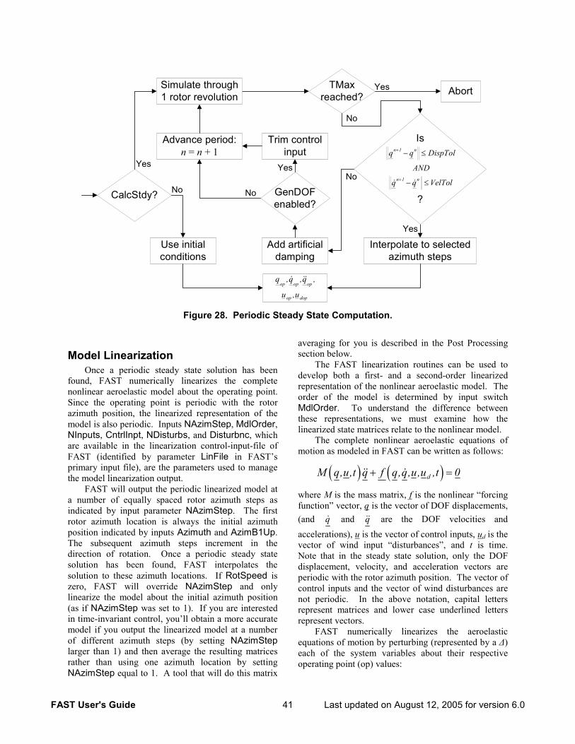
FAST User's Guide 41 Last updated on August 12, 2005 for version 6.0
Figure 28. Periodic Steady State Computation.
Model Linearization Once a periodic steady state solution has been
found, FAST numerically linearizes the complete nonlinear aeroelastic model about the operating point. Since the operating point is periodic with the rotor azimuth position, the linearized representation of the model is also periodic. Inputs NAzimStep, MdlOrder, NInputs, CntrlInpt, NDisturbs, and Disturbnc, which are available in the linearization control-input-file of FAST (identified by parameter LinFile in FAST’s primary input file), are the parameters used to manage the model linearization output.
FAST will output the periodic linearized model at a number of equally spaced rotor azimuth steps as indicated by input parameter NAzimStep. The first rotor azimuth location is always the initial azimuth position indicated by inputs Azimuth and AzimB1Up. The subsequent azimuth steps increment in the direction of rotation. Once a periodic steady state solution has been found, FAST interpolates the solution to these azimuth locations. If RotSpeed is zero, FAST will override NAzimStep and only linearize the model about the initial azimuth position (as if NAzimStep was set to 1). If you are interested in time-invariant control, you’ll obtain a more accurate model if you output the linearized model at a number of different azimuth steps (by setting NAzimStep larger than 1) and then average the resulting matrices rather than using one azimuth location by setting NAzimStep equal to 1. A tool that will do this matrix
averaging for you is described in the Post Processing section below.
The FAST linearization routines can be used to develop both a first- and a second-order linearized representation of the nonlinear aeroelastic model. The order of the model is determined by input switch MdlOrder. To understand the difference between these representations, we must examine how the linearized state matrices relate to the nonlinear model.
The complete nonlinear aeroelastic equations of motion as modeled in FAST can be written as follows:
( ) ( )dM q,u,t q f q,q,u,u ,t 0+ =
where M is the mass matrix, f is the nonlinear “forcing function” vector, q is the vector of DOF displacements, (and q and q are the DOF velocities and accelerations), u is the vector of control inputs, ud is the vector of wind input “disturbances”, and t is time. Note that in the steady state solution, only the DOF displacement, velocity, and acceleration vectors are periodic with the rotor azimuth position. The vector of control inputs and the vector of wind disturbances are not periodic. In the above notation, capital letters represent matrices and lower case underlined letters represent vectors.
FAST numerically linearizes the aeroelastic equations of motion by perturbing (represented by a ∆) each of the system variables about their respective operating point (op) values:
Interpolate to selectedazimuth steps
Add artificialdamping
Yes
Is
?
n 1 n
n 1 n
q q DispTol
AND
q q VelTol
+
+
− ≤
− ≤
Simulate through1 rotor revolution
Trim controlinput
No
Advance period:n = n + 1
GenDOFenabled?
No
Yes
CalcStdy?
Yes
Use initialconditions
No
op op op
op dop
q ,q ,q ,
u ,u
TMaxreached? Abort
No
Yes
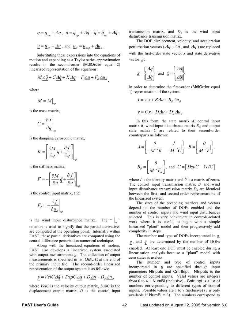
FAST User's Guide 42 Last updated on August 12, 2005 for version 6.0
opq q q∆= + ,
opq q q∆= + ,
opq q q∆= + ,
opu u u∆= + , and d dop du u u∆= + .
Substituting these expressions into the equations of motion and expanding as a Taylor series approximation results in the second-order (MdlOrder equal 2) linearized representation of the equations:
ddM q C q K q F u F u∆ ∆ ∆ ∆ ∆+ + = +,
where
opM M=
is the mass matrix,
op
fC
q∂
=∂
is the damping/gyroscopic matrix,
op
fMK qq q
∂∂= +
∂ ∂
is the stiffness matrix,
op
fMF qu u
∂ ∂= − + ∂ ∂
is the control input matrix, and
dd op
fF
u∂
= −∂
is the wind input disturbance matrix. The “op
” notation is used to signify that the partial derivatives are computed at the operating point. Internally within FAST, these partial derivatives are computed using the central difference perturbation numerical technique.
Along with the linearized equations of motion, FAST also develops a linearized system associated with output measurements y. The collection of output measurements is specified in list OutList at the end of the primary input file. The second-order linearized representation of the output system is as follows:
ddy VelC q DspC q D u D u∆ ∆ ∆ ∆= + + +
where VelC is the velocity output matrix, DspC is the displacement output matrix, D is the control input
transmission matrix, and Dd is the wind input disturbance transmission matrix.
The DOF displacement, velocity, and acceleration perturbation vectors ( q∆ , q∆ , and q∆ ) are replaced with the first-order state vector x and state derivative vector x :
qx
q
∆
∆ =
and q
xq
∆
∆ =
in order to determine the first-order (MdlOrder equal 1) representation of the system:
ddx Ax B u B u∆ ∆= + +
ddy C x D u D u∆ ∆= + +
In this form, the state matrix A, control input matrix B, wind input disturbance matrix Bd, and output state matrix C are related to their second-order counterparts as follows:
1 1
0 IA
M K M C− −
= − −
, 1
0B
M F−
=
,
d 1d
0B
M F−
=
, and [ ]C DspC VelC=
where I is the identity matrix and 0 is a matrix of zeros. The control input transmission matrix D and wind input disturbance transmission matrix Dd are identical between the first- and second-order representations of the linearized system.
The sizes of the preceding matrices and vectors depend on the number of DOFs enabled and the number of control inputs and wind input disturbances selected. This is very convenient in controls-related work where it is useful to begin with a simple linearized “plant” model and then progressively add complexity in steps.
The number and type of DOFs incorporated in q, q , and q are determined by the number of DOFs enabled. At least one DOF must be enabled during a linearization analysis because a “plant” model with zero states is useless.
The number and type of control inputs incorporated in u are specified through input parameters NInputs and CntrlInpt. NInputs is the number of control inputs. Valid values are integers from 0 to 4 + NumBl (inclusive). CntrlInpt is a list of numbers corresponding to different types of control inputs. Possible values are 1 to 7 (inclusive) (7 is only available if NumBl = 3). The numbers correspond to
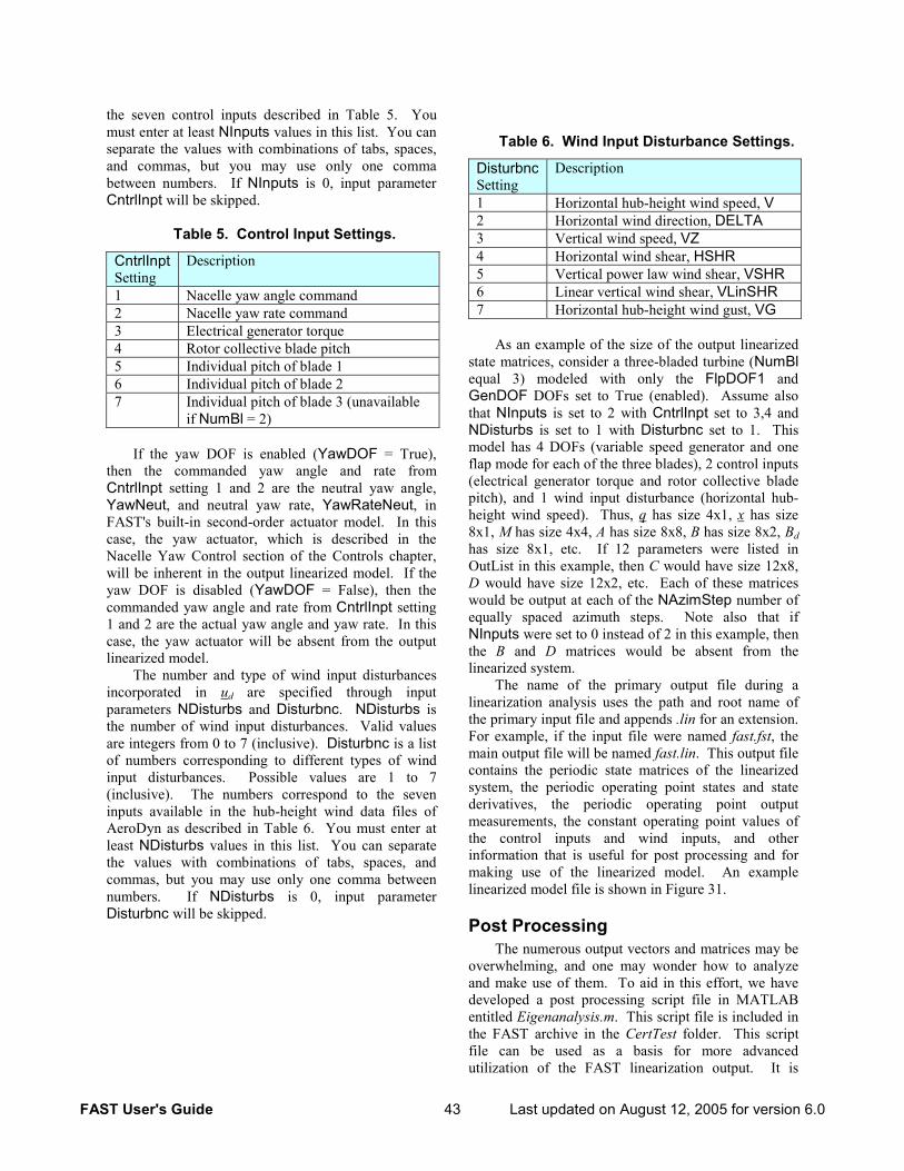
FAST User's Guide 43 Last updated on August 12, 2005 for version 6.0
the seven control inputs described in Table 5. You must enter at least NInputs values in this list. You can separate the values with combinations of tabs, spaces, and commas, but you may use only one comma between numbers. If NInputs is 0, input parameter CntrlInpt will be skipped.
Table 5. Control Input Settings.
CntrlInpt Setting
Description
1 Nacelle yaw angle command 2 Nacelle yaw rate command 3 Electrical generator torque 4 Rotor collective blade pitch 5 Individual pitch of blade 1 6 Individual pitch of blade 2 7 Individual pitch of blade 3 (unavailable
if NumBl = 2) If the yaw DOF is enabled (YawDOF = True),
then the commanded yaw angle and rate from CntrlInpt setting 1 and 2 are the neutral yaw angle, YawNeut, and neutral yaw rate, YawRateNeut, in FAST's built-in second-order actuator model. In this case, the yaw actuator, which is described in the Nacelle Yaw Control section of the Controls chapter, will be inherent in the output linearized model. If the yaw DOF is disabled (YawDOF = False), then the commanded yaw angle and rate from CntrlInpt setting 1 and 2 are the actual yaw angle and yaw rate. In this case, the yaw actuator will be absent from the output linearized model.
The number and type of wind input disturbances incorporated in ud are specified through input parameters NDisturbs and Disturbnc. NDisturbs is the number of wind input disturbances. Valid values are integers from 0 to 7 (inclusive). Disturbnc is a list of numbers corresponding to different types of wind input disturbances. Possible values are 1 to 7 (inclusive). The numbers correspond to the seven inputs available in the hub-height wind data files of AeroDyn as described in Table 6. You must enter at least NDisturbs values in this list. You can separate the values with combinations of tabs, spaces, and commas, but you may use only one comma between numbers. If NDisturbs is 0, input parameter Disturbnc will be skipped.
Table 6. Wind Input Disturbance Settings.
Disturbnc Setting
Description
1 Horizontal hub-height wind speed, V 2 Horizontal wind direction, DELTA 3 Vertical wind speed, VZ 4 Horizontal wind shear, HSHR 5 Vertical power law wind shear, VSHR 6 Linear vertical wind shear, VLinSHR 7 Horizontal hub-height wind gust, VG
As an example of the size of the output linearized
state matrices, consider a three-bladed turbine (NumBl equal 3) modeled with only the FlpDOF1 and GenDOF DOFs set to True (enabled). Assume also that NInputs is set to 2 with CntrlInpt set to 3,4 and NDisturbs is set to 1 with Disturbnc set to 1. This model has 4 DOFs (variable speed generator and one flap mode for each of the three blades), 2 control inputs (electrical generator torque and rotor collective blade pitch), and 1 wind input disturbance (horizontal hub-height wind speed). Thus, q has size 4x1, x has size 8x1, M has size 4x4, A has size 8x8, B has size 8x2, Bd has size 8x1, etc. If 12 parameters were listed in OutList in this example, then C would have size 12x8, D would have size 12x2, etc. Each of these matrices would be output at each of the NAzimStep number of equally spaced azimuth steps. Note also that if NInputs were set to 0 instead of 2 in this example, then the B and D matrices would be absent from the linearized system.
The name of the primary output file during a linearization analysis uses the path and root name of the primary input file and appends .lin for an extension. For example, if the input file were named fast.fst, the main output file will be named fast.lin. This output file contains the periodic state matrices of the linearized system, the periodic operating point states and state derivatives, the periodic operating point output measurements, the constant operating point values of the control inputs and wind inputs, and other information that is useful for post processing and for making use of the linearized model. An example linearized model file is shown in Figure 31.
Post Processing The numerous output vectors and matrices may be
overwhelming, and one may wonder how to analyze and make use of them. To aid in this effort, we have developed a post processing script file in MATLAB entitled Eigenanalysis.m. This script file is included in the FAST archive in the CertTest folder. This script file can be used as a basis for more advanced utilization of the FAST linearization output. It is
FAST User's Guide 44 Last updated on August 12, 2005 for version 6.0
written in MATLAB because MATLAB is the tool most commonly used in controls-related design work.
To run the Eigenanalysis.m script file, open a MATLAB command window, change the current working directory to the directory in which the script file is stored, and type “Eigenanalysis” into the MATLAB command prompt. The script file will prompt you for the name of the FAST linearization output file to process. Type only the root name of this file—omit the .lin extension. The name may optionally include an absolute or relative path if Eigenanalysis.m is not stored in the same directory as the FAST linearization output file. Naturally, a FAST linearization analysis must be run before the Eigenanalysis.m script file is run, and a linearization output file must be available for processing.
Running Eigenanalysis.m will cause MATLAB to read in the periodic state matrices from the FAST linearization output file. If the linearized model is second-order, the script will then compute the first-order state matrices from the second-order matrices using the equations documented above. If the linearized model is first-order, the script will not compute the second-order matrices from the first-order state matrices because the process cannot be reversed (there is no unique solution available without
knowledge of the mass matrix). The form of the state matrix A without damping (as if C were zero) is computed next. Azimuth-averaged matrices are then computed for all available periodic matrices. Finally, the script will perform an eigenanalysis on the periodic and azimuth-averaged state matrix A, with and without damping. The resulting eigenvalues and eigenvectors are the full system natural frequencies and mode shapes. The natural frequencies are available in both rad/sec and Hz.
After the script file has completed execution, type “who” into the MATLAB command prompt. This will cause MATLAB to list the available variables. The variable names are descriptive enough that they can be discerned without further documentation. For example, the azimuth-averaged full system natural frequencies of the nondamped system, in Hz, are available in variable FrequenciesAvgHzNoDamp. Their associated mode shapes are available in variable ModeShapesAvgNoDamp.
Please refer to MATLAB documentation for additional help on running MATLAB and learning commands that are useful for controls-related design work, which make use of linearized models output from FAST.
FAST User's Guide 45 Last updated on August 12, 2005 for version 6.0
ADAMS PREPROCESSOR
General Description FAST has the capability of extracting “equivalent”
ADAMS (Automatic Dynamic Analysis of Mechanical Systems) wind turbine datasets from the turbine properties specified in the FAST input file(s). That is, FAST has the functionality of acting like an ADAMS preprocessor capable of creating ADAMS datasets of wind turbine models through FAST’s simple property-input-style interface. Thus, FAST can be used as an alternative to the ADAMS/WT toolkit (12) or other preprocessors used to create ADAMS datasets of wind turbine models. The FAST to ADAMS preprocessor feature is enabled through the switch ADAMSPrep in the primary input file. This chapter, which describes the FAST to ADAMS preprocessor, assumes the reader is familiar with the basics of ADAMS.
The main advantages for using FAST to create ADAMS datasets are to ensure consistency between FAST and ADAMS models and to facilitate quick and easy creation of ADAMS datasets. The FAST-to-ADAMS preprocessor supports the mentality that all pertinent configuration information be stored in a single location (i.e., the FAST input files). The FAST to ADAMS preprocessor provides a natural progression from the medium-complexity FAST wind turbine models to the highly complex models possible using ADAMS. Once a working FAST model has been developed, little additional effort is required to create the more advanced ADAMS model. This is a useful way to impress your boss—you can accomplish a lot of work with very little effort.
The ADAMS datasets extracted from FAST contain all the functionality and usability associated with the FAST model, while bypassing some of FAST’s limitations. All the turbine control paradigms available in FAST, as discussed in the Controls chapter, are incorporated into the ADAMS model. These include the functionality of yawing the nacelle, pitching the blades, controlling the generator and HSS brake torque, and deploying the tip brakes. The ADAMS datasets incorporate the same generator, drivetrain compliance, nacelle yaw, rotor-furl, tail-furl, rotor teeter, and support platform models and DOFs used by FAST. Also, all of the output parameters specified at the end of FAST’s primary input file are passed into the ADAMS datasets. This eliminates the need to develop a REQSUB() user-written subroutine for request output every time an ADAMS dataset is generated. Once an ADAMS analysis is run, the format of the ADAMS output file containing time-series data is identical to that of the FAST format so
that post-processing techniques are compatible for the codes.
Additionally, the ADAMS interface is developed in such a way that all user-defined routines developed for FAST, including UserGen(), UserVSCont(), UserHSSBr(), UserPtfmLd(), UserTeet(), UserRFrl(), UserTFrl(), UserTFin(), UserYawCont(), and PitchCntrl(), can be linked with ADAMS just as easily as they can be with FAST. The routines do not need to be modified in any way for compatibility with ADAMS. The AeroDyn input files are also fully compatible between the FAST models and the associated, extracted ADAMS datasets.
One of FAST’s limitations that is bypassed by ADAMS is the assumed-mode approximation of the blades and tower. The blades and tower of the extracted ADAMS model are developed from FAST’s distributed mass and stiffness inputs using ADAMS’ conventional approach of modeling flexible members through a series of lumped masses connected by stiffness and damping FIELDs. Nevertheless, FAST’s valuable DOF-switching functionality is still available in the ADAMS model, so these flexibilities can be eliminated through a simple flag, just as they can be in FAST (in ADAMS the flexibilities are eliminated collectively, not one mode at a time).
Moreover, several characteristics not implemented in the FAST model are incorporated into the extracted ADAMS model. These include torsional and extensional DOFs for the blades and tower, flap/twist coupling in the blades, precurved and preswept blades, mass and elastic offsets for the blades, mass offsets for the tower, actuator dynamics for the blade pitch controls, graphical output capabilities, and others documented below.
Compiling and Linking ADAMS Using the extracted ADAMS datasets requires the
purchase and installation of the commercial ADAMS multibody-dynamics and analysis package. ADAMS is available from MSC.Software Corporation of Santa Ana, California. You will also need a compiler. For the PC, you should use the Compaq Visual Fortran compiler, but its predecessor, Digital Fortran, will also work.
Additionally, one must download the ADAMS to AeroDyn (A2AD) source files (13) and compile and link the ADAMS user-created dynamic-link-library (DLL). This is where the compiler is required.
The A2AD archive is available for download from our Web page http://wind.nrel.gov/designcodes/simulators/adams2ad/. The source files included in the archive, which are
FAST User's Guide 46 Last updated on August 12, 2005 for version 6.0
pertinent to creating the DLL needed to run the ADAMS datasets extracted from FAST, are as follows:
GFOSUB.f90 Contains an interface for the user-defined support platform loading model and routines that interface ADAMS to AeroDyn so that AeroDyn can provide ADAMS with aerodynamic forces on each blade element.
SENSUB.f90 Contains a routine to detect the occurrence of a successful forward time step. This is needed for the AeroDyn interface.
REQSUB_FAST.f90 Contains routines for calculating the desired ADAMS output as specified in FAST’s primary input file.
SFOSUB_FAST.f90 Contains a routine for implementing the generator and variable-speed control models and an interface for the user-defined rotor teeter, rotor-furl, and tail-furl spring and damper models.
VARSUB_FAST.f90 Contains a routine for computing the demand blade pitch angles and demand nacelle yaw angle and rate.
VFOSUB_FAST.f90 Contains routines for computing the tip-brake drag and tail fin aerodynamic forces.
Source files GFOSUB.f90 and SENSUB.f90 are the generic routines provided in the A2AD archive for interfacing any ADAMS model to AeroDyn. A good description of these files is provided in (13). GFOSUB.f90 had to be modified slightly in order to incorporate an interface to the user-defined support platform loading model contained in routine UserPtfmLd(). Source files REQSUB_FAST.f90, SFOSUB_FAST.f90, VARSUB_FAST.f90, and VFOSUB_FAST.f90 were written explicitly for running ADAMS datasets extracted from FAST.
Also included in the A2AD archive is a file named CompileLinkA2AD.bat. This is a DOS command script useful for compiling and linking the ADAMS DLL, named appropriately, ADAMS.dll. You will need to modify this script before you can run it on your PC. Open the script with your favorite editor. You will need to change the variables DF_LOC, A2AD_LOC, AD_LOC, and FAST_LOC. Set them so they point to the locations of Digital Fortran and the A2AD, AeroDyn, and FAST source files respectively. The location of the FAST source files is needed so that the
same user-defined routines developed for FAST, including UserGen(), UserVSCont(), UserHSSBr(), UserPtfmLd(), UserTeet(), UserRFrl(), UserTFrl(), UserTFin(), UserYawCont(), and PitchCntrl(), can be used with the ADAMS model as well.
Once these path variables are set, save the updated script and run it from a command prompt by simply typing its name. You can also run the script by double-clicking on it from Windows Explorer. Note that a file named newline.txt, which is also contained in the A2AD archive, must be located in the same directory as the CompileLinkA2AD.bat script in order for the script to work. The script will create ADAMS.dll. This one DLL can be used to run any ADAMS datasets extracted from FAST. In other words, you will only need to create ADAMS.dll once (unless you change any of the user-defined routines or source files).
Guidelines for Creating ADAMS Datasets
Here is the recommended procedure for creating ADAMS datasets using the FAST to ADAMS preprocessor:
Step 1. Create a working FAST model. Do this by specifying the desired settings in the FAST input files, running a simulation, and then verifying that the response predictions are reasonable.
One drawback to creating both FAST and ADAMS models from the same input file(s) is that if an error is made when inputting properties for a FAST model, the extracted ADAMS model will contain the same error. All redundancy checks available when FAST and ADAMS models are created independently are eliminated. To minimize resulting repercussions, make sure that the FAST model is in working order and is outputting reasonable response predictions before creating the ADAMS datasets.
Step 2. Update the FAST input files to include the additional input specifications required for creating ADAMS datasets.
The creation of ADAMS datasets using the FAST to ADAMS preprocessor requires the specification of additional parameters in the input file ADAMSFile. This file contains ADAMS-specific inputs related to the blade pitch actuators, graphical output capabilities, and other ADAMS-specific functionalities.
Furthermore, additional distributed blade and tower stiffness and inertial properties must be specified in the blade and tower input files. These are input by including additional columns of distributed data. For the blades, the additional columns are for distributed torsional and extensional stiffnesses, the distributed flap/twist coupling coefficient, distributed inertias, distributed offsets for identifying the reference axis for precurved and preswept blades, and distributed mass and elastic offsets. For the tower, the additional columns are for distributed torsional and extensional

FAST User's Guide 47 Last updated on August 12, 2005 for version 6.0
stiffnesses, distributed inertias, and distributed mass offsets. See the sample input files and the Input Files chapter for more details on these additional inputs.
Several input parameters are handled differently between FAST and the ADAMS preprocessor. Users of the FAST to ADAMS preprocessor should be aware of these differences.
The time step size input parameter, DT, is used by the ADAMS preprocessor to specify the maximum step size the integrator is allowed to take in the variable-step-size numerical-integration scheme that is used by ADAMS. Users of the ADAMS preprocessor should be aware that this is in slight contradiction to how DT is used to specify the constant time step size for the numerical integration scheme that is used by FAST.
Since the blade and tower models incorporated into the ADAMS datasets do not operate on the modal principle, input parameters associated with modal properties are naturally handled differently in the ADAMS preprocessor.
Blade flap and edge damping ratios incorporated in ADAMS FIELD statements are set equal to the same ratios used for the first flap and edge modes in FAST. These ratios are determined by inputs BldFlDmp(1) and BldEdDmp(1) in the blade input file(s). The value of input BldFlDmp(2) does not affect the creation of ADAMS datasets.
Likewise, tower fore-aft and side-to-side damping ratios incorporated in ADAMS FIELD statements are set equal to the same ratios used for the first fore-aft and side-to-side modes in FAST. These ratios are determined by inputs TwrFADmp(1) and TwrSSDmp(1) in the tower input files. The values of inputs TwrFADmp(2) and TwrSSDmp(2) do not affect the creation of ADAMS datasets.
Moreover, the modal stiffness tuner input parameters contained in the blade and tower data files are completely ignored by the ADAMS preprocessor.
Blade flexibility is controlled by enabling the first blade modes through input flags FlapDOF1 and EdgeDOF. Enabling blade flexibility enables all blade flap, edge, torsional, and extensional DOFs; conversely, disabling the flexibility removes all of these DOFs. When using the ADAMS extractor, the setting of FlapDOF1 must be identical to that of EdgeDOF to emphasize that the flap DOFs can’t be enabled without also enabling edge DOFs or vice-versa. The setting of input flag FlapDOF2 does not affect the creation of the ADAMS datasets.
Tower flexibility is controlled by enabling the first tower modes through input flags TwFADOF1 and TwSSDOF1. Enabling tower flexibility enables all tower fore-aft, side-to-side, torsional, and extensional DOFs, and conversely, disabling the flexibility removes all of these DOFs. When using the ADAMS extractor, the setting of TwFADOF1 must be identical to that of TwSSDOF1 to emphasize that the fore-aft
DOFs can’t be enabled without also enabling side-to-side DOFs or vice-versa. The setting of input flags TwFADOF2 and TwSSDOF2 do not effect the creation of the ADAMS datasets.
Support platform rotational DOFs are controlled by enabling input flags PtfmRDOF, PtfmPDOF, and PtfmYDOF. Due to the method ADAMS uses to implement the rotational DOFs, FAST cannot build an ADAMS dataset if one of the platform rotational DOFs is set differently than the other two. Thus, you must set PtfmRDOF, PtfmPDOF, and PtfmYDOF to the same value (i.e., all .True or all False). There is no restriction on which combination of support platform translational DOFs are enabled.
Additionally, some features available in FAST can’t be modeled in ADAMS. Thus, when creating ADAMS datasets using the FAST to ADAMS preprocessor, FAST will abort and not create the ADAMS dataset if any of these features are selected.
Mechanical gearbox efficiency losses are very difficult to model in ADAMS. Thus, GboxEff must be set to 100% when creating ADAMS datasets. Similarly, the physics of a gearbox whose LSS and HSS rotate in opposite directions are difficult to model in ADAMS. Thus, GBRevers must be set to False when creating ADAMS datasets.
The initial displacements of the blades and tower, specified using inputs OoPDefl, IPDefl, TTDspFA, and TTDspSS, must all be zero when creating ADAMS datasets. This is due to the difficulty involved in assembling an ADAMS dataset that contains deflected flexible members at the model definition phase. The initial teeter angle, TeetDefl, must also be set to zero when creating ADAMS datasets. This restriction exists since the generic GFOSUB.f90 routines provided in the A2AD archive will not read initial blade element data properly if TeetDefl is nonzero. All of the other initial conditions specified in FAST’s primary input file, including the initial rotor speed (RotSpeed), are incorporated in the ADAMS datasets.
Due to a restriction in ADAMS, the title line of FAST’s primary input file, the third line in the file, must not contain any of the characters “,”, “;”, “&”, or “!” when creating ADAMS datasets. This is because the title is stored as a STRING statement in the ADAMS datasets (used for providing header information in the primary output file) and because ADAMS STRING statements prohibit the use of these characters.
Sensible limits are placed on the number of blade and tower elements so that a reasonable numbering scheme could be implemented for ADAMS blade and tower PART, MARKER, and FIELD statements. This restriction is that neither TwrNodes nor BldNodes can be greater than 99.
FAST User's Guide 48 Last updated on August 12, 2005 for version 6.0
Finally, users of the FAST-to-ADAMS preprocessor should also be aware that the linearization control features and Simulink interface available in FAST are not available in the extracted ADAMS models.
Step 3. Run FAST with ADAMSPrep set at 2 or 3. When ADAMSPrep is set to 2, FAST creates the ADAMS datasets and stops. When ADAMSPrep is set to 3, FAST creates the ADAMS datasets and then proceeds to run the FAST simulation as well.
When running, FAST generates two ADAMS files as follows: <RootName>_ADAMS.adm The ADAMS dataset containing
statements that characterize the model configuration, analysis settings, and output.
<RootName>_ADAMS.acf The ADAMS command file
containing statements that enable DOFs and drive the time-marching simulation.
where RootName is the name of the primary input file. For example, if the input file were named fast.fst, the extracted ADAMS files will be named fast_ADAMS.adm and fast_ADAMS.acf.
An additional file named <RootName>_ADAMS_LIN.acf is generated when flag MakeLINacf is enabled in the ADAMSFile. This third file contains statements that drive an ADAMS/LINEAR eigenanalysis of the model. The eigenanalysis is performed with no gravity, rotor speed, damping, or aerodynamics, no matter how the associated inputs are otherwise specified in FAST’s input files.
If you want to change the ADAMS model properties or analysis settings, simply change the desired input properties in the FAST input file(s) and run FAST again to create the updated ADAMS datasets. This causes FAST to overwrite your old datasets if they are located in the same directory in which FAST is called. You never need to manually change the ADAMS datasets unless you want to change the ADAMS model to include features not supported by the FAST-to-ADAMS preprocessor.
Before running the ADAMS simulation, it may be beneficial to examine the model in ADAMS View to make sure the configuration is as expected. To do this, open ADAMS View, choose Import… from the File menu, and then browse and select the ADAMS dataset (.adm) of interest.
Running ADAMS Before running ADAMS, it is imperative that you
first understand FAST. This is because the extracted ADAMS datasets are considerably more complex than
their associated FAST models. Please refer to Step 1 of the previous section for additional information regarding this issue.
Using ADAMS.dll, an extracted ADAMS dataset, and an extracted ADAMS control/command file, you can run the ADAMS simulation using the Run Custom Solver prompts available in ADAMS Solver. Experienced users of ADAMS can also develop script files so that ADAMS.dll can be run from any directory without manually going through the ADAMS Solver prompts.
In order to get the ADAMS simulation to run smoothly and converge accurately, you will most likely need to play around with the time step size and integrator error. The FAST-to-ADAMS preprocessor automatically enters a default integrator error of 0.001 for all of the ADAMS INTEGRATOR/GSTIFF statements. This should be suitable for most simulations, but may require adjustment for some.
Please refer to (13) for additional hints on running ADAMS simulations.
ADAMS generates several output files. The primary output file of interest has a .plt (for plot) extension. This file contains the columns of time-series data with one column for each parameter that is requested in the primary input file. The format of this output file is identical to that of FAST’s .out file so that post-processing techniques are compatible for the codes. The other files created are generic ADAMS output files generated by ADAMS Solver. It may or may not be useful to review these.
When examining time-series data output from ADAMS, please be aware of the following limitations. If the tower is rigid, the tower base loads will all be output with zeros—unfortunately, we haven’t found a reason or workaround for this anomoly. Also, when outputting local span blade loads, be aware that the loads at the outboard strain gages will be under-predicted by ADAMS. This is because ADAMS lumps all of its mass at the center of each segment (rigid body inertia effects are also included), and thus, the mass of the segment in which the local span loads are output does not contribute to the local load. This difference shows most in the outboard part of the blade and becomes insignificant toward the root. Finally, be aware that the gyroscopic pitching moments induced when the nacelle yaws while the drivetrain is spinning will be over-predicted by ADAMS. This results from the fact that the HSS is lumped to the LSS in the ADAMS model. A detailed explanation of why this lumping affects the gyroscopic pitch moments is provided in (6).
If SaveGrphcs is enabled in ADAMSFile, ADAMS will also generate a graphics output file with a .gra extension. The graphics output file may be used to view an animation of the ADAMS simulation. To view the simulation, open ADAMS View, choose
FAST User's Guide 49 Last updated on August 12, 2005 for version 6.0
Import… from the File menu, and then browse and select the ADAMS graphics file of interest. Once loaded, the animation can be played by choosing Animation Controls… from the Review menu. When running many ADAMS simulations, it is beneficial to disable SaveGrphcs—ADAMS will not then generate the graphics output file and will run faster as a result.
When ADAMS is run using the control/command file for the ADAMS/LINEAR analysis, a results output file with a .res extension is generated. To animate the system mode shapes, open ADAMS View, choose Import… from the File menu, and then browse and select the ADAMS results file of interest. Once loaded, the system modes can be animated by choosing Linear Modes Controls… from the Review menu. If you only require a listing of the system natural frequencies, these results are written and can be retrieved from either the .out (output) or .msg (message) files automatically generated by ADAMS Solver.
Description of the Extracted ADAMS Datasets
This section documents qualitatively how the extracted ADAMS datasets are organized and how the various components of the wind turbine model are implemented in ADAMS. If you are interested in manually modifying the ADAMS datasets in order to incorporate features not available by the FAST-to-ADAMS preprocessor, it is important to review this section first. If you have no interest in learning how the various components of the wind turbine model are implemented in ADAMS, you may skip this section entirely.
To learn the exact details on how the ADAMS datasets are generated, see the file FAST2ADAMS.f90 in the FAST source code. This Fortran file contains three subroutines, one for generating each of the ADAMS files output by FAST.
In general, the ADAMS datasets generated by FAST employ the same PART and MARKER numbering conventions as recommended in (13). For reference, a complete listing of all of the ADAMS statements (PARTs, MARKERs, FIELDs, JOINTs, etc.) contained in the extracted ADAMS datasets is provided on our Web page http://wind.nrel.gov/ designcodes/adams2ad/FAST2ADAMSStatements .xls. However, not all extracted ADAMS datasets contain every statement documented in this spreadsheet—only statements that are needed are included. For example, if the generator speed is held fixed by disabling the generator DOF, then the SFORCE statement used to model an unneeded generator torque will not be included in the ADAMS dataset.
When examining the ADAMS datasets, it is important to note that the system units for all
statements in the ADAMS datasets are in kilonewtons, kilograms, meters, and seconds for the force, mass, length, and time units respectively. These are specified through the use of a UNITS statement. The acceleration of gravity, specified using an ACCGRAV statement, acts in the negative z-direction of the GROUND reference frame and MARKER.
The ADAMS dataset containing statements that characterize the model configuration, analysis settings, and output (the .adm file) is organized into five main sections. The first is a header section containing comments that identify the model name and describe how and when the dataset was created. The second section contains definitions of all model PART, MARKER, and GRAPHICS statements. The third section contains the constraint JOINT and MOTION statements, and the fourth section contains force definitions, including FIELD, FRICTION, SFORCE, VFORCE, GFORCE, and SPRINGDAMPER statements. The last section contains definitions of analysis settings and output.
In each section that contains model definition statements, the model is assembled from the ground up, from the support platform through the blade tip. So, for example, if you want to examine the tower FIELD statements, look at the statements near the beginning of the force definition section.
The ADAMS command (.acf) files contain commands used to drive the simulation. These include an INTEGRATOR statement and either SIMULATE/DYNAMICS or LINEAR/EIGENSOL commands, depending on the type of analysis performed. The .acf files also contain DEACTIVATE commands used to remove superfluous constraints and enable DOFs based on the specifications in the feature flags section of FAST’s primary input file. Additional details on this last point are provided at the end of this section.
Each tower and blade element is characterized by its own PART statement. The center of mass MARKERs of these PARTs are located at the same vertical (for tower) and radial (for blade) locations as the analysis nodes used in FAST. For blades, the transverse locations of the center of mass MARKERs are positioned with the reference axis and center-of-gravity offsets specified in the blade input file. For towers, the transverse locations of the center of mass MARKERs are identified using the distributed center-of-gravity offsets specified in the tower input file. Interconnecting each PART is a stiffness and damping FIELD statement. The FIELDs attach to the PARTs at elastic axis MARKERs, which are located in the same transverse planes as the center of mass MARKERs of each PART. For the blades, the transverse locations of the elastic axis MARKERs are identified using the distributed reference axis and elastic-axis offsets
FAST User's Guide 50 Last updated on August 12, 2005 for version 6.0
specified in the blade file, and for the tower, are assumed coincident with the tower axis.
Users should note that a flexible member (a blade or tower) with “N” analysis nodes, will be assembled using “N+1” FIELD statements. “N-1” of the FIELD statements are used to interconnect the “N” analysis nodes to each another. The “Nth” FIELD statement is used to cantilever node 1 to the flexible member’s rigid base. The “(N+1)th” FIELD statement is used to connect node “N” to the tip of the flexible member, which for the tower is the tower-top and for a blade is the tip brake. For blades with no tip brakes (indicated by setting the associated TipMass to zero), the DOFs associated with the outermost FIELD statement are never enabled.
The support platform, tower top, bed plate, nacelle, generator, HSS, LSS, teeter pin, hub, pitch plates, tip brakes, tail, and structure furling with the rotor are all modeled using rigid PART statements. Each of these PARTs contains several MARKERs for identifying various locations and directions.
In the graphics output, each tower and blade element is identified with its own unique GRAPHICS statement. Additional GRAPHICS statements are used to illustrate the rigid tower base, nacelle, gearbox, HSS, LSS, generator, hub, tail boom, and tail fin.
The yaw bearing is modeled with a revolute JOINT. Nacelle yaw demand angles and rates, arising from both advanced yaw control algorithms and override yaw maneuver specifications, are computed in VARSUB() and stored in VARIABLE statements. If necessary, based on settings in FAST’s primary input file, routine VARSUB() calls FAST’s user-defined yaw control routine, UserYawCont(). The difference between the yaw demand angle and actual yaw angle (yaw error) and the yaw demand rate and actual yaw rate (yaw rate error) is passed through a yaw actuator model that is implemented with an explicit function-based SFORCE statement. This is the same yaw actuator inherent in equivalent FAST models. If the yaw DOF is disabled, the yaw JOINT is “locked” using a steady MOTION statement, but the yaw DOF cannot be disabled if yaw control is enabled (the ADAMS preprocessor will abort if you try).
The rotor-furl bearing is modeled with a revolute JOINT. When RFrlMod is set to 1, the standard, linear compliance is modeled with a rotational SPRINGDAMPER statement and the nonlinear up- and down- spring and damper stops are modeled with explicit function-based SFORCE statements. When RFrlMod is set to 2, the user-defined rotor-furl spring and damper model provided in routine UserRFrl() is interfaced to ADAMS from routine SFOSUB(), which in turn, is called from an SFORCE statement. If the rotor-furl DOF is disabled, the rotor-furl JOINT is “locked” using a steady MOTION statement.
Likewise, the tail-furl bearing is modeled with a revolute JOINT. When TFrlMod is set to 1, the standard, linear compliance is modeled with a rotational SPRINGDAMPER statement and the nonlinear up- and down- spring and damper stops are modeled with explicit function-based SFORCE statements. When TFrlMod is set to 2, the user-defined tail-furl spring and damper model provided in routine UserTFrl() is interfaced to ADAMS from routine SFOSUB(), which in turn, is called from an SFORCE statement. If the tail-furl DOF is disabled, the tail-furl JOINT is “locked” using a steady MOTION statement.
Low-speed shaft compliance is modeled with a revolute JOINT and a rotational SPRINGDAMPER statement. When drivetrain rotational flexibility is disabled, the JOINT is “locked” with a zero-valued MOTION statement.
Drivetrain torque models, including both the generator models and variable-speed control models, are implemented with an SFORCE (1-component scalar force) statement that calls routine SFOSUB(). This routine implements each type of drivetrain torque model available in FAST. The parameters passed to SFOSUB() depend on the type of drivetrain torque model selected in FAST’s primary input file. If necessary, SFOSUB() will call the user-defined UserGen() or UserVSCont() routines.
The high-speed shaft brake is implemented with a preload-only FRICTION statement. Since the magnitude of the preload torque cannot be time-varying, the full friction torque is applied throughout the entire simulation. To negate the unwanted resistance before THSSBrDp, an SFORCE statement that calls SFOSUB() is used to apply a cancellation torque between the shaft and the nacelle. The SFOSUB() also applies the linear ramping component of the braking torque (over time increment HSSBrDT) when HSSBrMode is set to 1. Alternatively, SFOSUB() calls FAST’s user-defined HSS brake routine UserHSSBr() to determine the fraction of torque to cancel out when HSSBrMode is set to 2.
The teeter bearing is modeled with a revolute JOINT. When TeetMod is set to 1, the standard, nonlinear teeter spring and damper models are implemented with explicit function-based SFORCE statements. When TeetMod is set to 2, the user-defined teeter spring and damper model provided in routine UserTeet() is interfaced to ADAMS from routine SFOSUB(), which in turn, is called from an SFORCE statement. If the teeter DOF is disabled, the teeter JOINT is “locked” using a steady MOTION statement.
The blade pitch bearing is modeled with a revolute JOINT. Blade pitch demand angles, arising from both advanced pitch control algorithms and override pitch maneuver specifications, are computed in VARSUB()
FAST User's Guide 51 Last updated on August 12, 2005 for version 6.0
and stored in VARIABLE statements. If necessary, based on settings in FAST’s primary input file, routine VARSUB() calls FAST’s user-defined pitch control routine, PitchCntrl(). The difference between the pitch demand angle and actual pitch angle (pitch error) is passed through a pitch actuator model that is implemented with an explicit function-based SFORCE statement. If pitch is not actively controlled during the simulation, the pitch JOINT is “locked” using a steady MOTION statement.
As described in the A2AD User’s Guide (13), ADAMS is interfaced to AeroDyn through routines provided in the A2AD source file GFOSUB.f90. Routine GFOSUB(), which is contained in GFOSUB.f90, is called from GFORCE (6-component general force) statements placed in the ADAMS dataset. There is one GFORCE statement for each blade analysis node (or element) in every blade.
A GFORCE statement, together with the GFOSUB(), is also used to interface ADAMS with the user-defined support platform loading model, routine UserPtfmLd().
Tip-brake drag forces are modeled using VFORCE (3-component vector force) statements that call routine VFOSUB(). The VFOSUB() routine employs the same simple logic FAST uses for computing tip brake drag forces.
Tail fin aerodynamic loads are also modeled using a VFORCE (3-component vector force) statement that calls routine VFOSUB(). When TFinMod is set to 1, the VFOSUB() routine employs the same simple logic FAST uses for computing the tail fin aerodynamic loads. When TFinMod is set to 2, the user-defined tail fin aerodynamic model provided in routine UserTFin() is interfaced to ADAMS from routine VFOSUB().
All output parameter names, units, and identifiers are stored in the ADAMS dataset using ARRAY and STRING statements. These are read in by routines in
the A2AD source file REQSUB_FAST.f90 to determine which channels to output. Additional parameters needed for computing output data are passed to REQSUB(), a routine contained in file REQSUB_FAST.f90. Routine REQSUB() is, in turn, called using a REQUEST statement in the ADAMS dataset.
No matter which DOFs are enabled when generating the ADAMS datasets with the FAST-to-ADAMS preprocessor, the ADAMS dataset is always assembled so that it possesses no DOFs upon initiation. That is, all DOFs are essentially “locked” during the model-loading phase. This is achieved by placing fixed JOINTs between each PART of the flexible blades and tower, placing an ORIENTATION JOINT between the GROUND and support platform PART, and by specifying steady MOTION statements at all revolute JOINTs for the yaw, rotor-furl, tail-furl, teeter, shaft, and blade pitch bearings.
Once the simulation begins using the ADAMS command (.acf) file, the first time step is processed with all the DOFs “locked”. After the first time step, the selected DOFs are enabled by removing the superfluous MOTION, JPRIM, and fixed JOINT statements through the use of DEACTIVATE commands. Processing the first time step with zero DOFs ensures that the initial condition solution, which always precedes the first SIMULATE/DYNAMICS event, does not “kick” the system when the rotor is initially spinning at some nonzero-valued rate. Instead, the simulation always begins with no initial deflections. This technique essentially bypasses the startup problems pertaining to most ADAMS datasets as discussed in (13). The transient behavior associated with the startup of an ADAMS analysis, should be nearly identical to that associated with the startup of a corresponding FAST analysis.

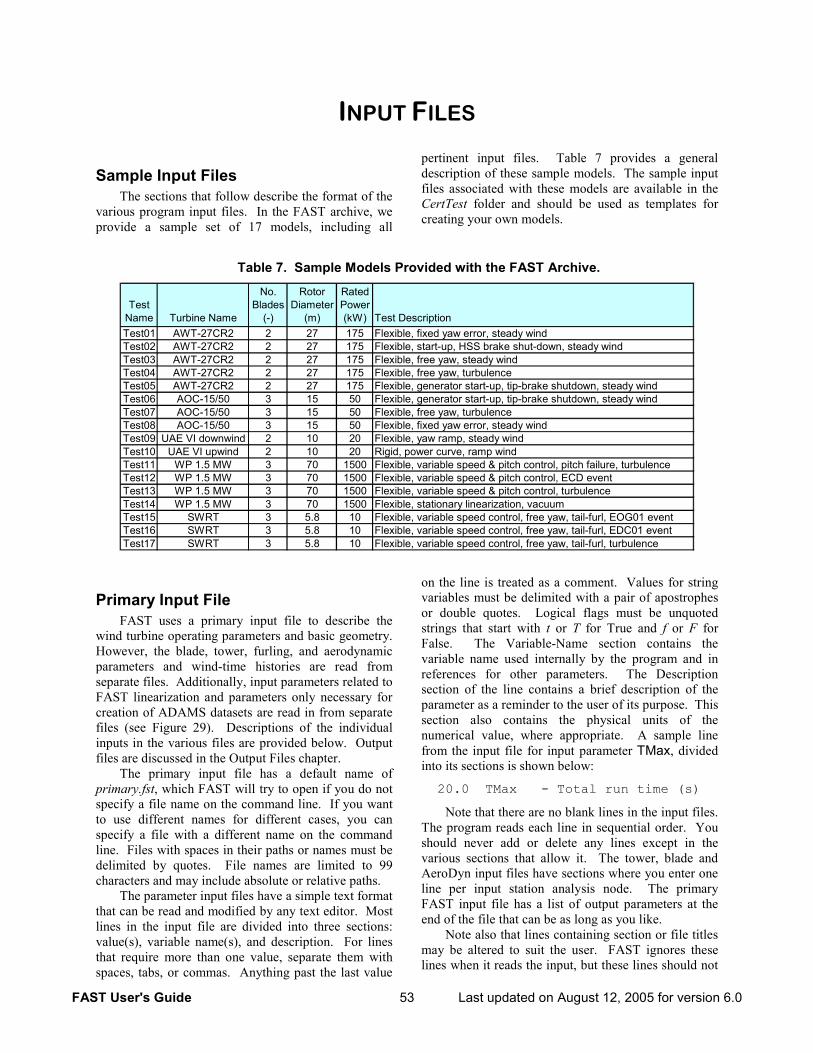
FAST User's Guide 53 Last updated on August 12, 2005 for version 6.0
INPUT FILES
Sample Input Files The sections that follow describe the format of the
various program input files. In the FAST archive, we provide a sample set of 17 models, including all
pertinent input files. Table 7 provides a general description of these sample models. The sample input files associated with these models are available in the CertTest folder and should be used as templates for creating your own models.
Table 7. Sample Models Provided with the FAST Archive.
Test Name Turbine Name
No. Blades
(-)
Rotor Diameter
(m)
Rated Power (kW) Test Description
Test01 AWT-27CR2 2 27 175 Flexible, fixed yaw error, steady windTest02 AWT-27CR2 2 27 175 Flexible, start-up, HSS brake shut-down, steady windTest03 AWT-27CR2 2 27 175 Flexible, free yaw, steady windTest04 AWT-27CR2 2 27 175 Flexible, free yaw, turbulenceTest05 AWT-27CR2 2 27 175 Flexible, generator start-up, tip-brake shutdown, steady windTest06 AOC-15/50 3 15 50 Flexible, generator start-up, tip-brake shutdown, steady windTest07 AOC-15/50 3 15 50 Flexible, free yaw, turbulenceTest08 AOC-15/50 3 15 50 Flexible, fixed yaw error, steady windTest09 UAE VI downwind 2 10 20 Flexible, yaw ramp, steady windTest10 UAE VI upwind 2 10 20 Rigid, power curve, ramp windTest11 WP 1.5 MW 3 70 1500 Flexible, variable speed & pitch control, pitch failure, turbulenceTest12 WP 1.5 MW 3 70 1500 Flexible, variable speed & pitch control, ECD eventTest13 WP 1.5 MW 3 70 1500 Flexible, variable speed & pitch control, turbulenceTest14 WP 1.5 MW 3 70 1500 Flexible, stationary linearization, vacuumTest15 SWRT 3 5.8 10 Flexible, variable speed control, free yaw, tail-furl, EOG01 eventTest16 SWRT 3 5.8 10 Flexible, variable speed control, free yaw, tail-furl, EDC01 eventTest17 SWRT 3 5.8 10 Flexible, variable speed control, free yaw, tail-furl, turbulence
Primary Input File FAST uses a primary input file to describe the
wind turbine operating parameters and basic geometry. However, the blade, tower, furling, and aerodynamic parameters and wind-time histories are read from separate files. Additionally, input parameters related to FAST linearization and parameters only necessary for creation of ADAMS datasets are read in from separate files (see Figure 29). Descriptions of the individual inputs in the various files are provided below. Output files are discussed in the Output Files chapter.
The primary input file has a default name of primary.fst, which FAST will try to open if you do not specify a file name on the command line. If you want to use different names for different cases, you can specify a file with a different name on the command line. Files with spaces in their paths or names must be delimited by quotes. File names are limited to 99 characters and may include absolute or relative paths.
The parameter input files have a simple text format that can be read and modified by any text editor. Most lines in the input file are divided into three sections: value(s), variable name(s), and description. For lines that require more than one value, separate them with spaces, tabs, or commas. Anything past the last value
on the line is treated as a comment. Values for string variables must be delimited with a pair of apostrophes or double quotes. Logical flags must be unquoted strings that start with t or T for True and f or F for False. The Variable-Name section contains the variable name used internally by the program and in references for other parameters. The Description section of the line contains a brief description of the parameter as a reminder to the user of its purpose. This section also contains the physical units of the numerical value, where appropriate. A sample line from the input file for input parameter TMax, divided into its sections is shown below:
20.0 TMax - Total run time (s)
Note that there are no blank lines in the input files. The program reads each line in sequential order. You should never add or delete any lines except in the various sections that allow it. The tower, blade and AeroDyn input files have sections where you enter one line per input station analysis node. The primary FAST input file has a list of output parameters at the end of the file that can be as long as you like.
Note also that lines containing section or file titles may be altered to suit the user. FAST ignores these lines when it reads the input, but these lines should not
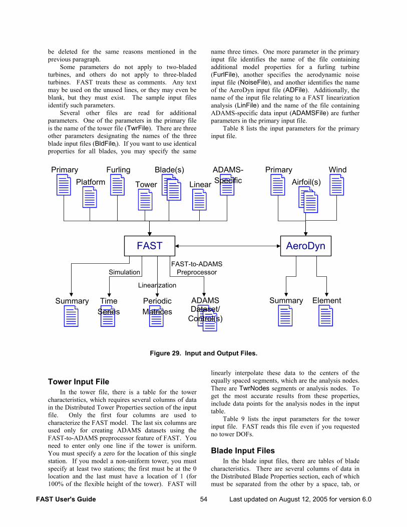
FAST User's Guide 54 Last updated on August 12, 2005 for version 6.0
be deleted for the same reasons mentioned in the previous paragraph.
Some parameters do not apply to two-bladed turbines, and others do not apply to three-bladed turbines. FAST treats these as comments. Any text may be used on the unused lines, or they may even be blank, but they must exist. The sample input files identify such parameters.
Several other files are read for additional parameters. One of the parameters in the primary file is the name of the tower file (TwrFile). There are three other parameters designating the names of the three blade input files (BldFilei). If you want to use identical properties for all blades, you may specify the same
name three times. One more parameter in the primary input file identifies the name of the file containing additional model properties for a furling turbine (FurlFile), another specifies the aerodynamic noise input file (NoiseFile), and another identifies the name of the AeroDyn input file (ADFile). Additionally, the name of the input file relating to a FAST linearization analysis (LinFile) and the name of the file containing ADAMS-specific data input (ADAMSFile) are further parameters in the primary input file.
Table 8 lists the input parameters for the primary input file.
Linearization
FAST AeroDyn
SimulationFAST-to-ADAMS
Preprocessor
Primary
Tower
Furling Primary
PeriodicMatrices
Element
Wind
Linear
ADAMS-Specific
TimeSeries
Blade(s)Airfoil(s)
ADAMSDataset/
Control(s)
Platform
Summary Summary
Figure 29. Input and Output Files.
Tower Input File In the tower file, there is a table for the tower
characteristics, which requires several columns of data in the Distributed Tower Properties section of the input file. Only the first four columns are used to characterize the FAST model. The last six columns are used only for creating ADAMS datasets using the FAST-to-ADAMS preprocessor feature of FAST. You need to enter only one line if the tower is uniform. You must specify a zero for the location of this single station. If you model a non-uniform tower, you must specify at least two stations; the first must be at the 0 location and the last must have a location of 1 (for 100% of the flexible height of the tower). FAST will
linearly interpolate these data to the centers of the equally spaced segments, which are the analysis nodes. There are TwrNodes segments or analysis nodes. To get the most accurate results from these properties, include data points for the analysis nodes in the input table.
Table 9 lists the input parameters for the tower input file. FAST reads this file even if you requested no tower DOFs.
Blade Input Files In the blade input files, there are tables of blade
characteristics. There are several columns of data in the Distributed Blade Properties section, each of which must be separated from the other by a space, tab, or
FAST User's Guide 55 Last updated on August 12, 2005 for version 6.0
comma. Only the first six columns are used to characterize the FAST model. The last 11 columns are used only for creating ADAMS datasets using the FAST-to-ADAMS preprocessor feature of FAST. You need to enter only one line if the blade is uniform. You must specify a zero for the location of this single station. If you model non-uniform blades, you must specify at least two stations; the first must be at the zero location and the last must have a location of 1 (for 100% span). FAST will linearly interpolate these data to the analysis nodes specified in the AeroDyn input file. There are BldNodes segments or analysis nodes. To get the most accurate results from these properties, include data points for the analysis nodes in the input table.
Table 10 lists the input parameters for the blade input files. FAST reads this file even if you requested no blade DOFs.
AeroDyn Input Files Table 11 lists the input parameters for the primary
AeroDyn input file. AeroDyn also uses other input files. The current version of AeroDyn accommodates two types of wind files. One type specifies hub-height wind data that also includes wind shears and gusts. You can use IECWind (14) or WindMaker (15) to generate these files for standard IEC wind conditions. You can also fabricate these simple text files from scratch or even use field-test data. The other type of wind file contains full-field wind data in a binary form. TurbSim (16), SNwind (17), or SNLWIND-3D (18) can generate these files. They contain two-dimensional grids of three-component winds that march past the turbine at a mean wind speed. AeroDyn also reads one or more files containing airfoil data.
Please see the AeroDyn user’s guide (1) for additional details on these files. FAST reads these files even if you disabled aerodynamic calculations.
Platform Input File Table 12 lists the input parameters for the platform
input data file. This file contains inputs related to the support platform configuration, motions, and loading.
FAST only reads the platform input file if PtfmModel from the primary input file is nonzero. In FAST v6.0, all nonzero PtfmModel options will work the same way by reading in the PtfmFile described in Table 12. In future versions, the format of this file will depend on which PtfmModel option is selected.
Furling Input File Table 13 lists the input parameters for the furling
input file. The inputs pertain to the lateral offset and skew angle of the rotor shaft, rotor-furling, tail-furling, and tail inertia and aerodynamics. If the turbine you want to model contains any of these characteristics, you must assemble the furling input file even if your turbine does not “furl” in the common sense of the word. For example, if the turbine you want to model contains a tail, you must assemble the furling input file regardless of whether or not your tail, or rotor, actively furls about the yawing-portion of the structure atop the tower.
It is clear that the inputs available in the furling input file define the core configuration of the turbine, just like those available in the primary input file. The reason we separated the parameters between the two input files is that the parameters available in the furling input are unique to small wind turbines. The challenge in defining the unique configurations of small wind turbines relative to the configurations of conventional machines is clearly demonstrated by the contents of the furling input file. Who said small wind turbines are easier to design than large wind turbines?
The furling input file is organized into sections similar to those available in the primary input file. This supports the notion that the furling file is simply a continuation and expansion of the core configuration-definition designations available in the primary file.
FAST only reads the furling input file if the model is designated as a furling machine (when Furling is set to True).
ADAMS-Specific Input File Table 14 lists the input parameters for the
ADAMS-specific-input data file. This file contains inputs related to the blade pitch actuators, graphical output capabilities, and other ADAMS-specific functionalities.
FAST does not read this file if ADAMS datasets are not generated (when ADAMSPrep is set to 1).
Linearization Control-Input File Table 15 lists the input parameters relating to a
FAST linearization analysis. FAST only reads in this file when performing a linearization analysis (when AnalMode is set to 2).
FAST User's Guide 56 Last updated on August 12, 2005 for version 6.0
Table 8. Primary-Input-File Parameters.
Simulation Control
Echo Setting this flag to True will cause FAST to echo input values as it reads them. It writes the data to the file echo.out. This is a useful tool to debug problems with your input files. For normal operation, set this parameter to False. (flag)
ADAMSPrep This switch determines whether or not the ADAMS preprocessor is enabled. Setting ADAMSPrep to 1 disables the ADAMS preprocessor and causes FAST to run its simulation as normal. A setting of 2 turns on the ADAMS preprocessor and turns off FAST; when FAST is run, the ADAMS datasets are created and FAST stops without performing a simulation. A setting of 3 enables both FAST and the ADAMS preprocessor; when FAST is run, the ADAMS datasets are created and FAST proceeds to run its simulation. Using values other than 1, 2, or 3 will cause FAST to abort. ADAMSPrep must be 1 when FAST is interfaced with Simulink. (switch)
AnalMode This switch determines whether to perform a time-marching analysis (simulation) or a linearization analysis (i.e., AnalMode stands for the analysis mode). A setting of 1 indicates a time-marching analysis. To perform a linearization analysis, set AnalMode to 2. Using values other than 1 or 2 will cause FAST to abort. AnalMode must be 1 when FAST is interfaced with Simulink. This input is not used in the FAST-to-ADAMS preprocessor. (switch)
NumBl This is the number of blades on the rotor. Valid values are 2 and 3. (-) TMax The overall simulation runtime. For time-marching simulations, the simulation stops when TMax
is reached. When computing a steady state solution during a linearization analysis, the iteration stops and FAST aborts if the solution has not converged by the time TMax is reached. (sec)
DT This is the time step for the constant-step-size numerical-integration scheme that is used by FAST. For ADAMS datasets extracted from FAST, DT is used to specify the maximum step size the integrator is allowed to take in the variable-step-size numerical-integration scheme that is used by ADAMS. You should be careful to choose an appropriate value for DT because if DT is too small or too large, the numerical solution will become unstable. Whenever you make changes to the configuration of your model, you should experiment with different values for DT and choose the largest value that does not affect your results. (sec)
Turbine Control
YCMode This is the yaw-control-mode switch for user-defined nacelle yaw control. Setting it to 0 disables user-defined yaw control. Setting it to 1 causes FAST to call a user-written routine called UserYawCont() at every time step past TYCOn. We supply a dummy routine in the software folder to help you write your own. Setting YCMode to 2 causes FAST to accept yaw position and rate demands externally from Simulink. The simple yaw maneuvers described below override the control setting determined by the user-supplied yaw controllers. Please see the Controls chapter for further details. YCMode must be 0 during a linearization analysis and must not be 2 unless FAST is interfaced with Simulink. Using values other than 0, 1, or 2 will cause FAST to abort. (switch)
TYCOn The time to enable active nacelle yaw control. This parameter is used only if YCMode is set to a non-zero value. TYCOn must not be negative and must equal zero when YCMode is 2. Please see the Controls chapter for further details. (sec)
PCMode This is the pitch-control-mode switch for user-defined pitch control. Setting it to 0 disables user-defined pitch control. Setting it to 1 causes FAST to call a user-written routine called PitchCntrl() at every time step past TPCOn. A real pitch-control routine created by Craig Hansen is linked with FAST, but we supply a dummy routine in the software folder to help you write your own. Setting PCMode to 2 causes FAST to accept pitch demands externally from Simulink. The simple pitch maneuvers described below override the control setting determined by the user-supplied pitch controllers. Please see the Controls chapter for further details. PCMode must be 0 during a linearization analysis and must not be 2 unless FAST is interfaced with Simulink. Using values other than 0, 1, or 2 will cause FAST to abort. (switch)
FAST User's Guide 57 Last updated on August 12, 2005 for version 6.0
Table 8. Primary-Input-File Parameters (continued).
Turbine Control (continued)
TPCOn The time to enable active pitch control. This parameter is used only if PCMode is set to a non-zero value. TPCOn must not be negative and must equal zero when PCMode is 2. Please see the Controls chapter for further details. (sec)
VSContrl This switch determines whether the generator torque is actively controlled for variable speed machines. The generator DOF flag, GenDOF, must be enabled to use this feature. Setting VSContrl to 0 will cause FAST to use one of the generator models defined by GenModel below to determine the generator torque. A setting of 1 for VSContrl will invoke a simple variable-speed model that uses the next four input parameters to determine the generator torque. Setting VSContrl to 2 will enable a user-written routine, UserVSCont(), to determine the generator torque. A sample routine is included in the file UserVSCont_KP.f90 and a dummy placeholder is available (and commented out) in UserSubs.f90. Setting VSContrl to 3 causes FAST to accept generator torque and electrical power demands externally from Simulink. VSContrl must not be 3 unless FAST is interfaced with Simulink. Using values other than 0, 1, 2, or 3 will cause FAST to abort. Please see the Controls chapter for further details. (switch)
VS_RtGnSp The simple variable-speed control changes from the Region 2½ (linear torque versus speed transition) to Region 3 (constant-torque control) at this generator speed (HSS speed). See Figure 22 for details. This value must not be less than zero, but it is ignored if VSContrl is not equal to 1. (rpm)
VS_RtTq This is the constant (or rated) torque applied to the HSS by the generator in Region 3 for the simple variable-speed controller. See Figure 22 for details. This value must not be less than zero, but it is ignored if VSContrl is not equal to 1. (N·m)
VS_Rgn2K When in Region 2 for the simple variable-speed controller, the generator speed is squared and multiplied by VS_Rgn2K to compute the generator torque to apply to the HSS. See Figure 22 for details. This value must not be less than zero, but it is ignored if VSContrl is not equal to 1. (N·m/rpm2)
VS_SlPc This is the rated generator slip percentage in the linear torque versus speed transition Region 2½ for the simple variable-speed controller. Similar to the simple induction generator input parameter SIG_SlPc, input VS_SlPc should be computed as the difference between the rated and the equivalent synchronous generator speed, divided by the equivalent synchronous speed, and then converted to percent. See Figure 22 for details. This value must greater than zero, but it is ignored if VSContrl is not equal to 1. (%)
GenModel This switch determines which generator model is used when GenDOF is enabled and VSContrl is set to 0. Setting it to 1 enables the simple-induction-generator model, whose parameters are defined in the Simple-Induction-Generator section below. Setting it to 2 enables the Thevenin-equivalent induction-generator model, whose parameters are defined in the Thevenin-Equivalent-Induction-Generator section below. Setting it to 3 will cause FAST to call the user-written subroutine, UserGen(). A UserGen() routine (found in UserVSCont_KP.f90), which calls routine UserVSCont() as if VSContrl was set to 2, is normally linked with the program and a dummy placeholder of UserGen() is also available (and commented out) in source file UserSubs.f90. In order to define your own generator model, you will need to write your own routine to replace it to use this option. Using values other than 1, 2, or 3 will cause FAST to abort. (switch)
GenTiStr This flag determines whether the generator is brought online at a specific time (TimGenOn) or a specific generator speed (SpGenOn). To use this feature, you must enable the generator DOF (GenDOF). GenTiStr must be True and TimGenOn must be 0.0 during a linearization analysis (AnalMod = 2) or when VSContrl is set to 3. (flag)
GenTiStp This flag determines whether the generator is taken offline at a specific time (TimGenOf) or when power falls to zero. To use this feature, you must enable the generator DOF (GenDOF). GenTiStp must be True and TimGenOf must greater than TMax during a linearization analysis (AnalMod = 2) or when VSContrl is set to 3. (flag)
SpGenOn If GenTiStr is False, the generator will switch on and stay on once the HSS speed reaches SpGenOn. This is used to do a speed startup of the generator. It applies to all generator models, including user-defined and variable-speed control. (rpm)
FAST User's Guide 58 Last updated on August 12, 2005 for version 6.0
Table 8. Primary-Input-File Parameters (continued).
Turbine Control (continued)
TimGenOn If GenTiStr is True, the generator will switch on at time TimGenOn. This is used to do a timed startup of the generator. It applies to all generator models, including user-defined and variable-speed control. GenTiStr must be True and TimGenOn must be 0.0 during a linearization analysis (AnalMod = 2) or when VSContrl is set to 3. (sec)
TimGenOf This parameter determines the time to turn off the generator when GenTiStp is True. This can be used for a shutdown maneuver or to simulate a loss of grid. This value is used whether you do a timed or speed-based startup. Normally, you won’t simulate a startup and a loss of grid (or shut-down) in the same run. In those cases, you will probably want to set this value to be greater than TMax. When you do want to use TimGenOf, you will probably want to enable GenTiStr and set TimGenOn to 0. TimGenOf must be greater than or equal to TimGenOn if GenTiStr is enabled. This parameter is not used if GenTiStp is False. In that case, the generator is taken offline when the power drops to zero. GenTiStp must be True and TimGenOf must greater than TMax during a linearization analysis (AnalMod = 2) or when VSContrl is set to 3. (sec)
HSSBrMode This switch determines which HSS brake model is used when GenDOF is enabled. Setting it to 1 enables the simple built-in HSS brake torque with a linear ramp-up from zero to HSSBrTqF over time HSSBrDT. Setting it to 2 causes FAST to call a user-written routine called UserHSSBr() at every time step past THSSBrDp. We supply a dummy routine in the software folder to help you write your own. Please see the Controls chapter for further details. Using values other than 1 or 2 will cause FAST to abort. (switch)
THSSBrDp At this time, the HSS brake will be deployed. In the simple model (HSSBrMode = 1), the braking torque will start its linear ramp to full torque, which happens after HSSBrDT seconds. In the user-defined model (HSSBrMode = 2), routine UserHSSBr() determines the fraction of full braking torque after deployment. You will probably want to turn the generator off a short time before this with TimGenOf before starting the HSS brake maneuver. THSSBrDp must greater than TMax during a linearization analysis (AnalMod = 2) or when FAST is interfaced with Simulink. (sec)
TiDynBrk The dynamic generator brake engages at this time. This input is CURRENTLY IGNORED since logic for the dynamic generator brake is not currently coded in FAST. TiDynBrk must greater than TMax during a linearization analysis. (sec)
TTpBrDpi The ith tip brake will start to deploy at this time. The drag constant for this brake will start to ramp up from TBDrConN to TBDrConD. You can specify different times for different brakes to simulate such conditions as one brake accidentally deploying or a situation in which one brake fails to deploy when commanded to do so. TTpBrDpi must greater than TMax during a linearization analysis. Only the first two values are used for two-bladed turbines. (sec)
TBDepISpi The ith tip brake will start to deploy when the rotor speed reaches TBDepISpi. Up to this point, the drag constant for the tip brake is TBDrConN. Once the tip brake starts to deploy, it will take TpBrDT seconds to reach full deployment, where it will remain deployed and using TBDrConD for the drag constant. During the TpBrDT second deployment, the drag constant for the tip brake will have an s-shaped ramp from TBDrConN to TBDrConD. TBDeplSpi must much greater than RotSpeed during a linearization analysis. Only the first two values are used for two-bladed turbines. (rpm)
TYawManS With or without yaw control or the yaw DOF enabled, after time TYawManS, the nacelle will yaw to NacYawF using a linear ramp from its current value at TYawManS until TYawManE. If yaw control is enabled when YCMode is not 0, the yaw commands determined from inputs TYawManS, TYawManE, and NacYawF override whatever commands come from the yaw controller. Also, the yaw commands determined from inputs TYawManS, TYawManE, and NacYawF pass through FAST’s built-in second-order actuator model if the yaw DOF is enabled when YawDOF is set to True. You can use TYawManS and TYawManE to simulate a yaw for startup, shutdown, or runaway yaw event. For a fixed-yaw simulation, set YawDOF to False, YCMode to 0, TYawManS greater than TMax, and NacYaw to the fixed nacelle yaw angle. TYawManS must greater than TMax during a linearization analysis. (sec)
TYawManE The nacelle yaw command will hold at a constant a setting of NacYawF from this time until the end of the run. TYawManE must be set larger or equal to TYawManS. (sec)
FAST User's Guide 59 Last updated on August 12, 2005 for version 6.0
Table 8. Primary-Input-File Parameters (continued).
Turbine Control (concluded)
NacYawF The nacelle yaw command will hold at a constant setting of NacYawF from TYawManE until the end of the run. (degrees)
TPitManSi With or without pitch control enabled, after time TPitManSi, the ith blade will pitch to BlPitchFi using a linear ramp from its current value at TPitManSi until TPitManEi. If pitch control is enabled when PCMode is not 0, the pitch commands determined from inputs TPitManSi, TPitManEi, and BlPitchFi override whatever commands come from the pitch controller. You can use TPitManSi and TPitManEi to simulate a pitch for startup, shutdown, or runaway pitch event. By setting one blade different from the other(s), you can simulate a fault condition in which one blade unexpectedly pitches or fails to pitch. For a constant-pitch simulation, set PCMode to 0, TPitManSi greater than TMax, and BlPitchi to the fixed blade pitch angles. TPitManSi must greater than TMax during a linearization analysis. Only the first two values are used for two-bladed turbines. (sec)
TPitManEi The ith blade will hold at a constant a setting of BlPitchFi from this time until the end of the run. TPitManEi must be set larger or equal to TPitManSi. Only the first two values are used for two-bladed turbines. (sec)
BlPitchi When PCMode is 0 during a time-marching analysis or if TrimCase is 1 or 2 while computing a steady state solution during a linearization analysis, the ith blade will hold at a constant setting of BlPitchi until TPitManSi. If PCMode is not 0 or if TrimCase is 3 while computing a steady state solution during a linearization analysis, BlPitchi is the initial pitch. The pitch angle is relative to the chord line at the point of zero aerodynamic twist and is positive towards feather (leading edge upwind). These values must be greater than –180 and less than or equal to 180 degrees. Only the first two values are used for two-bladed turbines. (deg)
BlPitchFi The ith blade will hold at a constant setting of BlPitchFi from TPitManEi until the end of the run. This is relative to the chord line at the point of zero aerodynamic twist and is positive towards feather (leading edge upwind). Only the first two values are used for two-bladed turbines. (deg)
Environmental Conditions
Gravity The gravitational acceleration constant. (m/sec2)
Feature Flags*
FlapDOF1 The first flapwise blade-bending mode will be enabled when this flag is True. When enabled, you should ensure that the corresponding mode shape specified in the blade input files is accurate. For ADAMS datasets extracted from FAST, this flag is used to enable or disable blade flexibility and its value must be identical to that of EdgeDOF. (flag)
FlapDOF2 The second flapwise blade-bending mode will be enabled when this flag is True. It is possible to enable the second mode without enabling the first mode, but it should be done only for research purposes. When enabled, you should ensure that the corresponding mode shape specified in the blade input files is accurate. The value of this input does not effect the creation of ADAMS datasets. (flag)
EdgeDOF The first edgewise blade-bending mode will be enabled when this flag is True. When enabled, you should ensure that the corresponding mode shape specified in the blade input files is accurate. For ADAMS datasets extracted from FAST, this flag is used to enable or disable blade flexibility and its value must be identical to that of FlapDOF1. (flag)
TeetDOF This flag enables rotor teetering when set to True. If this option is disabled, teeter can be set to any fixed angle. This flag is ignored for three-bladed turbines. (flag)
* You must enable at least one DOF during a linearization analysis (AnalMode set to 2). During a time-marching analysis (AnalMode set to 1), there is no restriction.
FAST User's Guide 60 Last updated on August 12, 2005 for version 6.0
Table 8. Primary-Input-File Parameters (continued).
Feature Flags (concluded)
DrTrDOF If set to True, this flag will enable torsional flexibility of the drivetrain. This models the drivetrain between the generator and rotor as a lumped torsion spring and damper. (flag)
GenDOF The generator DOF will be enabled when this flag is True. This allows use of the various variable-speed control schemes and generator models during a time-marching analysis or a trim solution during a linearization analysis. If False, the HSS will rotate at a fixed rate (RotSpeed*GBRatio). (flag)
YawDOF When set to True, this flag enables the nacelle yaw DOF. The initial nacelle yaw angle is specified with NacYaw. If YawDOF is disabled, the yaw angle will be fixed at NacYaw. (flag)
TwFADOF1 The first tower fore-aft bending mode will be enabled when this variable is set to True. When en-abled, you should ensure that the corresponding mode shape specified in the tower input file is ac-curate. For ADAMS datasets extracted from FAST, this flag is used to enable or disable tower flexibility and its value must be identical to that of TwSSDOF1. (flag)
TwFADOF2 The second tower fore-aft bending mode will be enabled when this variable is set to True. Except for research purposes, this flag should be set to True only if TwFADOF1is True. When enabled, you should ensure that the corresponding mode shape specified in the tower input file is accurate. The value of this input does not effect the creation of ADAMS datasets. (flag)
TwSSDOF1 The first tower side-to-side bending mode will be enabled when this variable is set to True. When enabled, you should ensure that the corresponding mode shape specified in the tower input file is accurate. For ADAMS datasets extracted from FAST, this flag is used to enable or disable tower flexibility and its value must be identical to that of TwFADOF1. (flag)
TwSSDOF2 The second tower side-to-side bending mode will be enabled when this variable is set to True. Ex-cept for research purposes, this flag should be set to True only if TwSSDOF1 is True. When en-abled, you should ensure that the corresponding mode shape specified in the tower input file is ac-curate. The value of this input does not effect the creation of ADAMS datasets. (flag)
CompAero This flag determines whether aerodynamic loads will be computed using the AeroDyn aerodynamic modules. If False, the simulation will occur in a vacuum (no airloads). AeroDyn input properties are specified in the ADFile (see input below). The ADFile must exist even if CompAero is False, since RNodes determines the location of the structural analysis points. (flag)
CompNoise A series of semi-empirical aeroacoustic noise prediction algorithms has been incorporated into FAST by Pat Moriarty of NREL/NWTC. The algorithms predict six different forms of aerodynamically produced noise including turbulent inflow, turbulent boundary layer trailing edge, separating flow, laminar boundary layer vortex shedding, trailing edge bluntness vortex shedding, and tip vortex formation. These noise sources are then superimposed to calculate and output the total aerocoustic signature of an operating wind turbine. CURRENTLY, THE NOISE PREDICTION INTERFACE IS NOT DOCUMENTED IN THIS GUIDE (except as it effects the primary-input-file). Details on the contents and validation of the aeroacoustic noise prediction models are provided in [19]. Questions related to the noise prediction models and interface should be directed to Pat Moriarty, preferably at night or on weekends .
The CompNoise flag determines whether aerodynamic noise will be computed. Aerodynamic noise input properties are specified in the NoiseFile (see input below). CompAero must be enabled if CompNoise is enabled. CompNoise must be False during a linearization analysis. The value of this input does not effect the creation of ADAMS datasets since the aeroacoustic algorithms are not linked to ADAMS. (flag)
FAST User's Guide 61 Last updated on August 12, 2005 for version 6.0
Table 8. Primary-Input-File Parameters (continued).
Initial Conditions
OoPDefl This is the initial, out-of-plane, blade-tip displacement. The same value is used for all blades. Note that by specifying values for initial conditions close to the steady-state conditions, the numerical solution technique will reach trimmed conditions faster. It is positive downwind. It is possible to specify combinations of tip displacements that are not meaningful for the blade structural pretwist distribution and the DOFs that are enabled. If so, FAST will issue a warning message and choose meaningful values for you. The value of OoPDefl must be zero (no initial deflection) when creating ADAMS datasets or when FAST is interfaced with Simulink. (m)
IPDefl This is the initial, in-plane, blade-tip displacement. The same value is used for all blades. Note that by specifying values for initial conditions close to the steady-state conditions, the numerical solution technique will reach “trimmed conditions” faster. It is positive clockwise when looking upwind. It is possible to specify combinations of tip displacements that are not meaningful for the blade structural pretwist distribution and the DOFs that are enabled. If so, FAST will issue a warning message and choose meaningful values for you. The value of IPDefl must be zero (no initial deflection) when creating ADAMS datasets or when FAST is interfaced with Simulink. (m)
TeetDefl This is the initial or fixed teeter angle. It is positive when Blade 1 is deflected downwind of the rotor. This value must be greater than –180 and less than or equal to 180 degrees and must be zero when creating ADAMS datasets. This parameter is ignored for three-bladed turbines. (deg)
Azimuth This is the initial azimuth angle for Blade 1. Please note that for three-bladed rotors, blade 3 is ahead of blade 2, which is ahead of blade 1, so that the order of blades passing through a given azimuth is 3-2-1-repeat. Azimuth works in conjunction with AzimB1Up, which is input in the Turbine Configuration section that follows. This value must be greater or equal to 0 and less than 360 degrees. (deg)
RotSpeed This is the initial angular speed of the rotor. During a linearization analysis, this is also the desired azimuth-average rotor speed for a trim solution. This value must not be negative. The turbine rotates clockwise when looking downwind. (rpm)
NacYaw This is the initial or fixed nacelle yaw angle. It is positive counterclockwise when looking down on the turbine. This value must be greater than –180 and less than or equal to 180 degrees. (deg)
TTDspFA This is the initial fore-aft tower-top displacement. It is positive downwind. The value of TTDspFA must be zero (no initial deflection) when creating ADAMS datasets or when FAST is interfaced with Simulink. (m)
TTDspSS This is the initial side-to-side tower-top displacement. It is positive to the right when looking upwind. The value of TTDspSS must be zero (no initial deflection) when creating ADAMS datasets or when FAST is interfaced with Simulink. (m)
Turbine Configuration
TipRad The blade-tip radius is the distance from the apex of the cone of rotation to the blade tip along the pitch axis instead of the perpendicular distance from the axis of rotation. See Figure 14(a) and Figure 16. This value must be greater than zero. (m)
HubRad The hub radius is the distance from the apex of the cone of rotation to the blade root along the pitch axis instead of the perpendicular distance from the axis of rotation. The blade root loads are defined at this radial span location. See Figure 14(b) and Figure 16. This value must be greater than or equal to zero and less than TipRad. (m)
PSpnElN This is the blade element number corresponding to the innermost blade element that is part of the pitchable portion of the blade for partial-span pitch control. The pitch of all the blade elements from PSpnElN to BldNodes are controlled by the BlPitch(:) array, whereas all the blade elements from 1 to (PSpnElN - 1) are not pitchable. Note that PSpnElN is CURRENTLY IGNORED by FAST; that is, the logic for partial-span pitch control has not yet been codified in FAST. This value must be an integer between 1 and BldNodes (inclusive). (-)
UndSling The undersling is the distance from the teeter pin to the apex of the cone of rotation. It is positive upwind. This parameter is ignored for three-bladed turbines. See Figure 14(b). (m)
HubCM This is the distance from the rotor apex to the hub mass center. It is positive downwind. See Figure 14(b) and Figure 16. (m)
FAST User's Guide 62 Last updated on August 12, 2005 for version 6.0
Table 8. Primary-Input-File Parameters (continued).
Turbine Configuration (concluded)
OverHang This is the distance along the rotor shaft from the yn-/zn-plane to the teeter pin for two-bladed turbines or from the yn-/ zn-plane to the rotor apex for three-bladed turbines. It is positive downwind, so use a negative number for upwind turbines. For turbines with rotor-furl, this distance defines the configuration at a furl angle of zero. See Figure 14(a), Figure 16, and Figure 18. (m)
NacCMxn This is the downwind distance to the nacelle mass center (reference input NacMass) from the top of the tower, measured parallel to the xn-axis. It is positive downwind. See Figure 14(a) and Figure 16. (m)
NacCMyn This is the lateral distance to the nacelle mass center (reference input NacMass) from the top of the tower, measured parallel to the yn-axis. It is positive to the left when looking downwind or positive into the page of Figure 14(a) and Figure 16. (m)
NacCMzn This is the vertical distance to the nacelle mass center (reference input NacMass) from the top of the tower, measured parallel to the zn-axis. It is positive upward when looking downwind. See Figure 14(a) and Figure 16. (m)
TowerHt The tower height is the distance from ground level [onshore] or mean sea level [offshore] to the top of the tower and yaw bearing. This value must be greater than zero. See Figure 14(a), Figure 16, and Figure 20. (m)
Twr2Shft This is the vertical distance from the top of the tower and yaw bearing to the intersection of the rotor shaft axis and the yn-/zn-plane. The distance is measured parallel to the zn-axis. See Figure 14(a), Figure 16, and Figure 18. The combination of TipRad, TowerHt, Twr2Shft, OverHang, and ShftTilt must ensure that the blade tip does not hit the ground. This value also cannot be negative. For turbines with rotor-furl, this distance defines the configuration at a furl angle of zero. (m)
TwrRBHt The tower rigid base height is the distance from tower base to the beginning of the flexible portion of the tower. The tower base loads are defined at this elevation. This value must be greater or equal to zero and less than TowerHt + TwrDraft. (m)
ShftTilt This is the tilt angle of the rotor shaft from the nominally horizontal plane. Positive tilt means that the downwind end of the shaft is the highest. This value must be between –90 and 90 degrees. Upwind turbines have negative tilt for improved tower clearance. For turbines with rotor-furl, this angle defines the configuration at a furl angle of zero. See Figure 14(a), Figure 16, and Figure 18. (deg)
Delta3 This teeter pin orientation angle allows coupling between the flapping due to teeter and blade pitch. A positive value means that the blade that teeters downwind has a positive change in pitch (leading edge upwind). See Figure 15 and the discussion on page 13 for details. This value must be between –90 and 90 degrees (exclusive) and is ignored for three-bladed turbines. (deg)
PreConei The coning angle for the ith blade is positive downwind for upwind and downwind rotors. See Figure 14(a) and Figure 16. These values must be greater than –180 and less than or equal to 180 degrees. Only the first two values are used for two-bladed turbines. (deg)
AzimB1Up All input and output azimuth values are measured with respect to this number. If this value is 0 and the rotor azimuth is 180 degrees, then Blade 1 is pointing down. Please keep in mind that the rotor rotates clockwise when looking downwind, so an azimuth value of 90 degrees means Blade 1 is pointing to the right (looking downwind) when AzimB1Up is 0. If AzimB1Up is 270 degrees and Azimuth is 0 degrees, then Blade 1 is to the right when looking downwind. Also note that for three-bladed rotors, blade 3 is ahead of blade 2, which is ahead of blade 1, so that the order of blades passing through a given azimuth is 3-2-1-repeat. (deg)
FAST User's Guide 63 Last updated on August 12, 2005 for version 6.0
Table 8. Primary-Input-File Parameters (continued).
Mass and Inertia
YawBrMass This is the mass of the yaw bearing. Its center is located at the top of the tower, at the origin of the tower-top/base-plate and nacelle/yaw coordinate systems. This value must not be negative. (kg)
NacMass This is the mass of the nacelle. The center of the nacelle mass is located at the point specified by inputs NacCMxn, NacCMyn, and NacCMzn relative to the tower-top. It includes everything atop the tower excluding the rotor (blades, hub, and tip brakes), yaw bearing, and systems that furl (tail boom, tail fin, and structure furling with the rotor). This value must not be negative. (kg)
HubMass This is the mass of the hub. Its center is located a distance of HubCM from the rotor apex. This value must not be negative. (kg)
TipMassi This is the tip-brake mass for the ith blade. This value must not be negative. Only the first two values are used for two-bladed turbines. (kg)
NacYIner This is the nacelle moment of inertia about the yaw axis. It includes all mass contained in NacMass. This value must be greater than NacMass•( NacCMxn2 + NacCMyn2 ). (kg·m2)
GenIner This is the moment of inertia of the high-speed portion of the drivetrain including the gearbox, HSS, and generator. If torsional flexibility of the drivetrain is enabled, the compliance is between the inertia of the rotor and this inertia. This value will be multiplied by the square of the gear ratio to map it to the low-speed reference frame. This value must not be negative. (kg·m2)
HubIner The hub moment of inertia is measured about the teeter axis for two-bladed turbines or about the rotor shaft axis for three-bladed turbines. For two-bladed turbines, it includes those parts that teeter, except for the blades and tip brakes, and must be greater than HubMass•( UndSling – HubCM )2. For three-bladed turbines, it excludes the blades and tip brakes and must not be negative. (kg·m2)
Drivetrain
GBoxEff The gearbox efficiency is the ratio of the output shaft power to the input shaft power. Enter it as a percentage from 0 to 100. The value of GboxEff must be 100 (no mechanical losses) when creating ADAMS datasets. (%)
GenEff The generator efficiency is the ratio of its output power to its input power. It is used by the simple-induction-generator model (GenModel = 1) to obtain the electrical power from the mechanical power, which is a product of the generator torque and HSS speed. It is also used by the simple variable-speed, generator torque controller (VSContrl = 1) in the same manor. Enter it as a percentage from 0 to 100. GenEff is ignored by the Thevenin-equivalent induction-generator model (GenModel = 2), which incorporates a more complex expression for the electrical power based on the input circuit resistances. The value of GenEff is passed to UserGen() and UserVSCont() for the user-defined generator model (GenModel = 3) and user-defined variable-speed, generator torque controller (VSContrl = 2) respectively, but the user-defined models allow for the flexibility of implementing any relationship between input and output power. (%)
GBRatio This is the ratio of the HSS speed to the LSS speed. This value must be greater than zero and should be 1.0 for a direct-drive turbine. (-)
GBRevers Set this value to True if the direction of rotation of the LSS is opposite that of the HSS. GBRevers must be set to False when creating ADAMS datasets. (flag)
HSSBrTqF This maximum mechanical brake torque value is applied to the HSS end of the drivetrain compliance. This value must not be negative. It is used by both the simple (HSSBrMode = 1) and user-defined (HSSBrMode = 2) HSS brake models. (N·m)
HSSBrDT For the simple HSS brake model (HSSBrMode = 1), this is the amount of time it takes the HSS brake to reach full torque once it is applied. The ramp from off to full torque is linear. This value must not be negative and is unused when HSSBrMode is set to 2. (sec)
DynBrkFi This is name of a file containing a curve of mechanical generator torques versus HSS speeds defining the dynamic generator brake characteristics. The name may optionally include an absolute or relative path. This file name must contain fewer than 100 characters and must be enclosed in apostrophes or double quotes. This input is CURRENTLY IGNORED since logic for the dynamic generator brake is not currently coded in FAST. (-)
FAST User's Guide 64 Last updated on August 12, 2005 for version 6.0
Table 8. Primary-Input-File Parameters (continued).
Drivetrain (concluded)
DTTorSpr The equivalent drive-train torsional spring constant includes compliance in the LSS, the gearbox, and the HSS. This value must not be negative. (N·m/rad)
DTTorDmp The equivalent drive-train torsional damping constant includes compliance in the LSS, the gearbox, and the HSS. This value must not be negative. (N·m/sec)
Simple Induction Generator
SIG_SlPc The rated generator slip percentage is the difference between the rated and the synchronous generator speed divided by the synchronous generator speed, and then converted to percent. See Figure 12 for details. This value must be greater than zero, but it is ignored if GenModel is not equal to 1 or VSContrl is not equal to 0. (%)
SIG_SySp This is the synchronous or zero-torque generator speed. See Figure 12 for details. This value must be greater than zero, but it is ignored if GenModel is not equal to 1 or VSContrl is not equal to 0. (rpm)
SIG_RtTq This is the torque supplied by the generator when running at rated speed. See Figure 12 for de-tails. This value must be greater than zero, but it is ignored if GenModel is not equal to 1 or VSContrl is not equal to 0. (N·m)
SIG_PORt The pullout ratio is the ratio of the pullout torque and the rated torque. The negative of this value is also used for the startup torque. See Figure 12 for details. This value must be greater than or equal to one, but it is ignored if GenModel is not equal to 1 or VSContrl is not equal to 0. (-)
Thevenin-Equivalent, 3-Phase, Induction Generator
TEC_Freq This is the line frequency of the electrical grid. This value must be greater than zero and should be 50 (Europe) or 60 (U.S.), but it is ignored if GenModel is not equal to 2 or VSContrl is not equal to 0. (Hz)
TEC_NPol This is the number of poles in the generator. This value must be an even integer greater than zero, but it is ignored if GenModel is not equal to 2 or VSContrl is not equal to 0. (-)
TEC_SRes This is the resistance of the generator stator in the complete circuit. This value must be greater than zero, but it is ignored if GenModel is not equal to 2 or VSContrl is not equal to 0. (ohms)
TEC_RRes This is the resistance of the generator rotor in the complete circuit. This value must be greater than zero, but it is ignored if GenModel is not equal to 2 or VSContrl is not equal to 0. (ohms)
TEC_VLL This is the line-to-line voltage of the generator. This value must be greater than zero and is often 690 in Europe or 480 or 575 in the U.S., but it is ignored if GenModel is not equal to 2 or VSContrl is not equal to 0. (volts)
TEC_SLR This is the leakage reactance of the generator stator in the complete circuit. This value must be greater than zero, but it is ignored if GenModel is not equal to 2 or VSContrl is not equal to 0. It is usually a small number and is close in value to the stator resistance. (ohms)
TEC_RLR This is the leakage reactance of the generator rotor in the complete circuit. This value must be greater than zero, but it is ignored if GenModel is not equal to 2 or VSContrl is not equal to 0. It is usually a small number and is close in value to the rotor resistance. (ohms)
TEC_MR This is the magnetizing reactance of the complete generator circuit. This value must be greater than zero, but it is ignored if GenModel is not equal to 2 or VSContrl is not equal to 0. It is usually about 10-50 times greater than the leakage reactances. (ohms)

FAST User's Guide 65 Last updated on August 12, 2005 for version 6.0
Table 8. Primary-Input-File Parameters (continued).
Platform Model
PtfmModel This is a switch used to indicate the type of support platform and to tell FAST whether or not to read in an additional file of inputs for defining the model properties of the support platform (see next input PtfmFile). The additional inputs in PtfmFile pertain to the to the support platform configuration, motions, and loading. Setting PtfmModel to 1 specifies an onshore foundation. Setting it to 2 specifies a fixed bottom offshore foundation. Setting it to 3 specifies a floating offshore configuration. Setting PtfmModel to 0 disables the platform models—in this case, FAST will rigidly attach the tower to the inertia frame (ground) through a cantilever connection. Using values other than 0, 1, 2, or 3 will cause FAST to abort.
PtfmFile This is the name of the file that contains additional model properties for the support platform. The name may optionally include an absolute or relative path. This file name must contain fewer than 100 characters and must be enclosed in apostrophes or double quotes. FAST will only read this file if PtfmModel is nonzero. See Table 12 for a listing of input parameters contained in this file. In FAST v6.0, all nonzero PtfmModel options will work the same way by reading in PtfmFile. In future versions, the format of this file will depend on which PtfmModel option is selected. (quoted string)
Tower
TwrNodes The tower is divided into TwrNodes equal-length segments. The nodes at the centers of these segments are used for the integration of elastic forces. The more segments you use, the more accurate the integral will be, but the greater the computational time will be. A good compromise for this parameter is 20. This value must be an integer greater than 0. When creating ADAMS datasets, this value must be no more than 99. (-)
TwrFile This is the name of the file that contains the tower properties. The name may optionally include an absolute or relative path. This file name must contain fewer than 100 characters and must be enclosed in apostrophes or double quotes. FAST will read this file even when there are no tower DOFs. See Table 9 for a listing of input parameters contained in this file. (quoted string)
Nacelle Yaw
YawSpr This is the torsional spring stiffness in FAST’s built-in, second-order, nacelle yaw actuator model. The linear nacelle-yaw spring moment is proportional to the nacelle-yaw error through this constant. If a yaw actuator natural frequency is known in place of an actuator spring stiffness, compute the spring stiffness as follows: YawSpr = YawIner•ωn
2, where ωn is the natural frequency in rad/sec and YawIner is the nominal inertia of the nacelle, rotor, and tail about the yaw axis in kg·m2. This value must not be negative. (N·m/rad)
YawDamp This is the torsional damping constant in FAST’s built-in, second-order, nacelle yaw actuator model. The linear nacelle-yaw damping moment is proportional to the nacelle-yaw rate error through this constant. If a yaw actuator natural frequency and damping ratio are known in place of an actuator damping constant, compute the damping constant as follows: YawDamp = 2•ζ•YawIner•ωn, where ωn is the natural frequency in rad/sec, ζ is the damping ratio in fraction of critical, and YawIner is the nominal inertia of the nacelle, rotor, and tail about the yaw axis in kg·m2. This value must not be negative. (N·m/(rad/sec))
YawNeut When YCMode is 0, this is the neutral nacelle yaw position (constant yaw command) as described on page 12. When YCMode is not zero, this is the initial, constant yaw command before active yaw control is enabled at time TYCOn. This value must be greater than –180 and less than or equal to 180 degrees. (deg)
FAST User's Guide 66 Last updated on August 12, 2005 for version 6.0
Table 8. Primary-Input-File Parameters (continued).
Furling
Furling This flag is used to tell FAST whether or not to read in an additional file of inputs for defining the model configuration of a furling turbine (see next input FurlFile). The additional inputs in FurlFile pertain to the lateral offset and skew angle of the rotor shaft, rotor-furling, tail-furling, and tail inertia and aerodynamics. If the turbine you want to model contains any of these characteristics, you must assemble the furling input file even if your turbine does not “furl” in the common sense of the word. For example, if the turbine you want to model contains a tail, you must assemble the furling input file regardless of whether or not your tail, or rotor, actively furls about the yawing-portion of the structure atop the tower. (flag)
FurlFile This is the name of the file that contains additional model properties for a furling turbine. The name may optionally include an absolute or relative path. This file name must contain fewer than 100 characters and must be enclosed in apostrophes or double quotes. FAST will only read this file if the model is designated as a furling machine (when Furling is set to True). See Table 13 for a listing of input parameters contained in this file. (quoted string)
Rotor Teeter
TeetMod The teeter springs and dampers can be modeled three ways. For a value of 0 for TeetMod, there will be no teeter spring nor damper and the moment normally produced will be set to zero. A TeetMod of 1 will invoke simple spring and damper models using the inputs provided below as appropriate coefficients. If you set TeetMod to 2, FAST will call the routine UserTeet() to compute the teeter spring and damper moments. You should replace the dummy routine supplied with the code with your own, which will need to be linked with the rest of FAST. Using values other than 0, 1, or 2 will cause FAST to abort. This parameter is ignored for three-bladed turbines. (switch)
TeetDmpP The teeter damper is effective when the teeter deflection exceeds this value. This value must be between 0 and 180 degrees (inclusive). This parameter is ignored for three-bladed turbines and when TeetMod is not set to 1. (deg)
TeetDmp The linear teeter damping moment is proportional to the teeter rate through this constant and is effective when the teeter deflection exceeds TeetDmpP. This value must not be negative. This parameter is ignored for three-bladed turbines and when TeetMod is not set to 1. (N·m/(rad/sec))
TeetCDmp The Coulomb-friction damping moment resists teeter motion, but it is a constant that is not proportional to the teeter rate. However, if the teeter rate is zero, the damping is zero. This value must not be negative. This parameter is ignored for three-bladed turbines and when TeetMod is not set to 1. (N·m)
TeetSStP The teeter soft-stop spring is effective when the teeter deflection exceeds this value. This value must be between 0 and 180 degrees (inclusive). This parameter is ignored for three-bladed turbines and when TeetMod is not set to 1. (deg)
TeetHStP The teeter hard-stop spring is effective when the teeter deflection exceeds this value. This value must be between TeetSStP and 180 degrees (inclusive). This parameter is ignored for three-bladed turbines and when TeetMod is not set to 1. (deg)
TeetSSSp The linear teeter soft-stop spring restoring moment is proportional to the teeter soft-stop deflection by this constant and is effective when the teeter deflection exceeds TeetSStP. This value must not be negative. This parameter is ignored for three-bladed turbines and when TeetMod is not set to 1. (N·m/rad)
TeetHSSp The linear teeter hard-stop spring restoring moment is proportional to the teeter hard-stop deflection by this constant and is effective when the teeter deflection exceeds TeetHStP. This value must not be negative. This parameter is ignored for three-bladed turbines and when TeetMod is not set to 1. (N·m/rad)
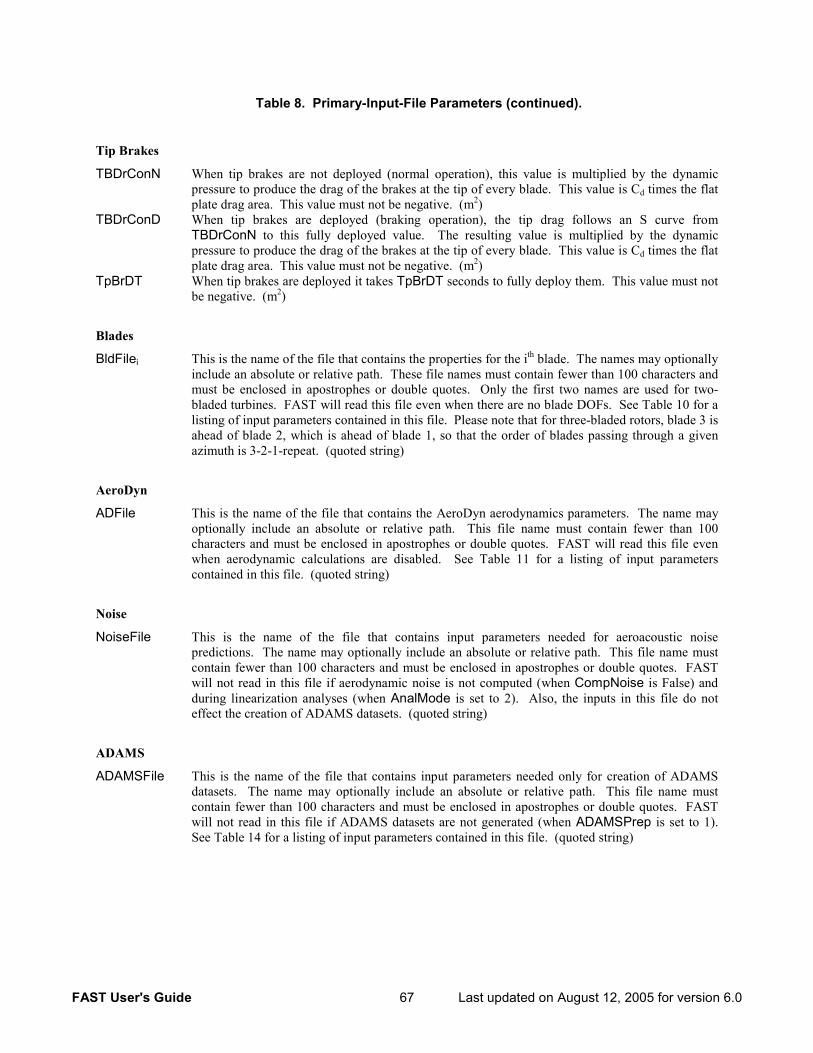
FAST User's Guide 67 Last updated on August 12, 2005 for version 6.0
Table 8. Primary-Input-File Parameters (continued).
Tip Brakes
TBDrConN When tip brakes are not deployed (normal operation), this value is multiplied by the dynamic pressure to produce the drag of the brakes at the tip of every blade. This value is Cd times the flat plate drag area. This value must not be negative. (m2)
TBDrConD When tip brakes are deployed (braking operation), the tip drag follows an S curve from TBDrConN to this fully deployed value. The resulting value is multiplied by the dynamic pressure to produce the drag of the brakes at the tip of every blade. This value is Cd times the flat plate drag area. This value must not be negative. (m2)
TpBrDT When tip brakes are deployed it takes TpBrDT seconds to fully deploy them. This value must not be negative. (m2)
Blades
BldFilei This is the name of the file that contains the properties for the ith blade. The names may optionally include an absolute or relative path. These file names must contain fewer than 100 characters and must be enclosed in apostrophes or double quotes. Only the first two names are used for two-bladed turbines. FAST will read this file even when there are no blade DOFs. See Table 10 for a listing of input parameters contained in this file. Please note that for three-bladed rotors, blade 3 is ahead of blade 2, which is ahead of blade 1, so that the order of blades passing through a given azimuth is 3-2-1-repeat. (quoted string)
AeroDyn
ADFile This is the name of the file that contains the AeroDyn aerodynamics parameters. The name may optionally include an absolute or relative path. This file name must contain fewer than 100 characters and must be enclosed in apostrophes or double quotes. FAST will read this file even when aerodynamic calculations are disabled. See Table 11 for a listing of input parameters contained in this file. (quoted string)
Noise
NoiseFile This is the name of the file that contains input parameters needed for aeroacoustic noise predictions. The name may optionally include an absolute or relative path. This file name must contain fewer than 100 characters and must be enclosed in apostrophes or double quotes. FAST will not read in this file if aerodynamic noise is not computed (when CompNoise is False) and during linearization analyses (when AnalMode is set to 2). Also, the inputs in this file do not effect the creation of ADAMS datasets. (quoted string)
ADAMS
ADAMSFile This is the name of the file that contains input parameters needed only for creation of ADAMS datasets. The name may optionally include an absolute or relative path. This file name must contain fewer than 100 characters and must be enclosed in apostrophes or double quotes. FAST will not read in this file if ADAMS datasets are not generated (when ADAMSPrep is set to 1). See Table 14 for a listing of input parameters contained in this file. (quoted string)
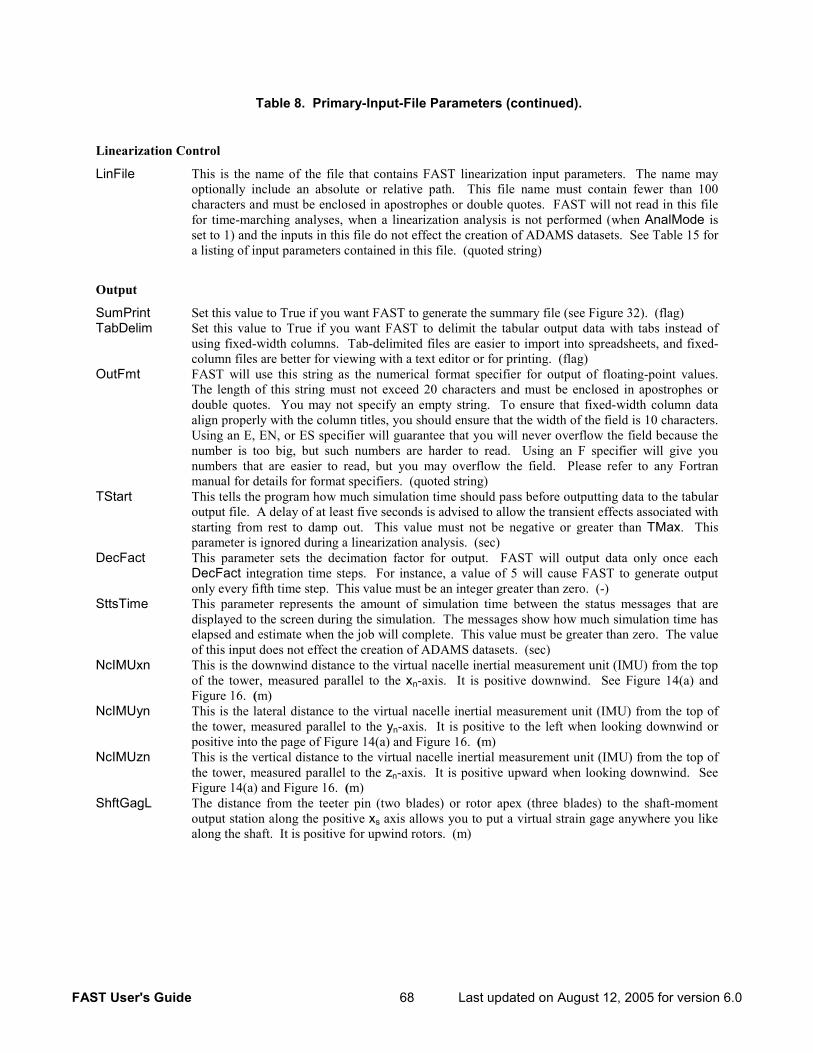
FAST User's Guide 68 Last updated on August 12, 2005 for version 6.0
Table 8. Primary-Input-File Parameters (continued).
Linearization Control
LinFile This is the name of the file that contains FAST linearization input parameters. The name may optionally include an absolute or relative path. This file name must contain fewer than 100 characters and must be enclosed in apostrophes or double quotes. FAST will not read in this file for time-marching analyses, when a linearization analysis is not performed (when AnalMode is set to 1) and the inputs in this file do not effect the creation of ADAMS datasets. See Table 15 for a listing of input parameters contained in this file. (quoted string)
Output
SumPrint Set this value to True if you want FAST to generate the summary file (see Figure 32). (flag) TabDelim Set this value to True if you want FAST to delimit the tabular output data with tabs instead of
using fixed-width columns. Tab-delimited files are easier to import into spreadsheets, and fixed-column files are better for viewing with a text editor or for printing. (flag)
OutFmt FAST will use this string as the numerical format specifier for output of floating-point values. The length of this string must not exceed 20 characters and must be enclosed in apostrophes or double quotes. You may not specify an empty string. To ensure that fixed-width column data align properly with the column titles, you should ensure that the width of the field is 10 characters. Using an E, EN, or ES specifier will guarantee that you will never overflow the field because the number is too big, but such numbers are harder to read. Using an F specifier will give you numbers that are easier to read, but you may overflow the field. Please refer to any Fortran manual for details for format specifiers. (quoted string)
TStart This tells the program how much simulation time should pass before outputting data to the tabular output file. A delay of at least five seconds is advised to allow the transient effects associated with starting from rest to damp out. This value must not be negative or greater than TMax. This parameter is ignored during a linearization analysis. (sec)
DecFact This parameter sets the decimation factor for output. FAST will output data only once each DecFact integration time steps. For instance, a value of 5 will cause FAST to generate output only every fifth time step. This value must be an integer greater than zero. (-)
SttsTime This parameter represents the amount of simulation time between the status messages that are displayed to the screen during the simulation. The messages show how much simulation time has elapsed and estimate when the job will complete. This value must be greater than zero. The value of this input does not effect the creation of ADAMS datasets. (sec)
NcIMUxn This is the downwind distance to the virtual nacelle inertial measurement unit (IMU) from the top of the tower, measured parallel to the xn-axis. It is positive downwind. See Figure 14(a) and Figure 16. (m)
NcIMUyn This is the lateral distance to the virtual nacelle inertial measurement unit (IMU) from the top of the tower, measured parallel to the yn-axis. It is positive to the left when looking downwind or positive into the page of Figure 14(a) and Figure 16. (m)
NcIMUzn This is the vertical distance to the virtual nacelle inertial measurement unit (IMU) from the top of the tower, measured parallel to the zn-axis. It is positive upward when looking downwind. See Figure 14(a) and Figure 16. (m)
ShftGagL The distance from the teeter pin (two blades) or rotor apex (three blades) to the shaft-moment output station along the positive xs axis allows you to put a virtual strain gage anywhere you like along the shaft. It is positive for upwind rotors. (m)
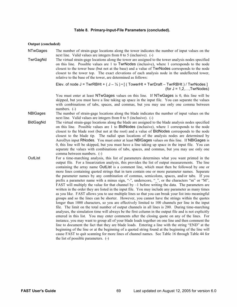
FAST User's Guide 69 Last updated on August 12, 2005 for version 6.0
Table 8. Primary-Input-File Parameters (concluded).
Output (concluded)
NTwGages The number of strain-gage locations along the tower indicates the number of input values on the next line. Valid values are integers from 0 to 5 (inclusive). (-)
TwrGagNd The virtual strain-gage locations along the tower are assigned to the tower analysis nodes specified on this line. Possible values are 1 to TwrNodes (inclusive), where 1 corresponds to the node closest to the tower base (but not at the base) and a value of TwrNodes corresponds to the node closest to the tower top. The exact elevations of each analysis node in the undeflected tower, relative to the base of the tower, are determined as follows:
Elev. of node J = TwrRBHt + ( J – ½ ) • [ ( TowerHt + TwrDraft – TwrRBHt ) / TwrNodes ] (for J = 1,2,…,TwrNodes)
You must enter at least NTwGages values on this line. If NTwGages is 0, this line will be skipped, but you must have a line taking up space in the input file. You can separate the values with combinations of tabs, spaces, and commas, but you may use only one comma between numbers. (-)
NBlGages The number of strain-gage locations along the blade indicates the number of input values on the next line. Valid values are integers from 0 to 5 (inclusive). (-)
BldGagNd The virtual strain-gage locations along the blade are assigned to the blade analysis nodes specified on this line. Possible values are 1 to BldNodes (inclusive), where 1 corresponds to the node closest to the blade root (but not at the root) and a value of BldNodes corresponds to the node closest to the blade tip. The radial span locations of the analysis nodes are determined by AeroDyn input RNodes. You must enter at least NBlGages values on this line. If NBlGages is 0, this line will be skipped, but you must have a line taking up space in the input file. You can separate the values with combinations of tabs, spaces, and commas, but you may use only one comma between numbers. (-)
OutList For a time-marching analysis, this list of parameters determines what you want printed in the output file. For a linearization analysis, this provides the list of output measurements. The line containing the array name OutList is a comment line, which must then be followed by one or more lines containing quoted strings that in turn contain one or more parameter names. Separate the parameter names by any combination of commas, semicolons, spaces, and/or tabs. If you prefix a parameter name with a minus sign, “-”, underscore, “_”, or the characters “m” or “M”, FAST will multiply the value for that channel by –1 before writing the data. The parameters are written in the order they are listed in the input file. You may include any parameter as many times as you like. FAST allows you to use multiple lines so that you can break your list into meaningful groups and so the lines can be shorter. However, you cannot have the strings within the quotes longer than 1000 characters, so you are effectively limited to 100 channels per line in the input file. The limit on the total number of output channels in all lines is 200. During time-marching analyses, the simulation time will always be the first column in the output file and is not explicitly entered in this list. You may enter comments after the closing quote on any of the lines. For instance, you may want to group all of your blade loads together on one line and then comment the line to document the fact that they are blade loads. Entering a line with the string “END” at the beginning of the line or at the beginning of a quoted string found at the beginning of the line will cause FAST to quit scanning for more lines of channel names. See Table 16 through Table 44 for the list of possible parameters. (-)
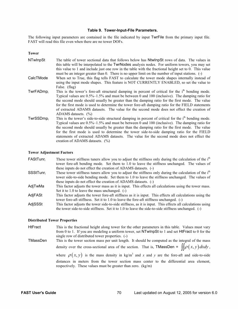
FAST User's Guide 70 Last updated on August 12, 2005 for version 6.0
Table 9. Tower-Input-File Parameters.
The following input parameters are contained in the file indicated by input TwrFile from the primary input file. FAST will read this file even when there are no tower DOFs.
Tower
NTwInpSt The table of tower sectional data that follows below has NtwInpSt rows of data. The values in this table will be interpolated to the TwrNodes analysis nodes. For uniform towers, you may set this value to 1 and include just one row in the table with the fractional height set to 0. This value must be an integer greater than 0. There is no upper limit on the number of input stations. (-)
CalcTMode When set to True, this flag tells FAST to calculate the tower mode shapes internally instead of using the input mode shapes. This feature is NOT CURRENTLY ENABLED, so set the value to False. (flag)
TwrFADmpi This is the tower’s fore-aft structural damping in percent of critical for the ith bending mode. Typical values are 0.5%–1.5% and must be between 0 and 100 (inclusive). The damping ratio for the second mode should usually be greater than the damping ratio for the first mode. The value for the first mode is used to determine the tower fore-aft damping ratio for the FIELD statements of extracted ADAMS datasets. The value for the second mode does not effect the creation of ADAMS datasets. (%)
TwrSSDmpi This is the tower’s side-to-side structural damping in percent of critical for the ith bending mode. Typical values are 0.5%–1.5% and must be between 0 and 100 (inclusive). The damping ratio for the second mode should usually be greater than the damping ratio for the first mode. The value for the first mode is used to determine the tower side-to-side damping ratio for the FIELD statements of extracted ADAMS datasets. The value for the second mode does not effect the creation of ADAMS datasets. (%)
Tower Adjustment Factors
FAStTunri These tower stiffness tuners allow you to adjust the stiffness only during the calculation of the ith tower fore-aft bending mode. Set them to 1.0 to leave the stiffness unchanged. The values of these inputs do not effect the creation of ADAMS datasets. (-)
SSStTunri These tower stiffness tuners allow you to adjust the stiffness only during the calculation of the ith tower side-to-side bending mode. Set them to 1.0 to leave the stiffness unchanged. The values of these inputs do not effect the creation of ADAMS datasets. (-)
AdjTwMa This factor adjusts the tower mass as it is input. This effects all calculations using the tower mass. Set it to 1.0 to leave the mass unchanged. (-)
AdjFASt This factor adjusts the tower fore-aft stiffness as it is input. This effects all calculations using the tower fore-aft stiffness. Set it to 1.0 to leave the fore-aft stiffness unchanged. (-)
AdjSSSt This factor adjusts the tower side-to-side stiffness, as it is input. This effects all calculations using the tower side-to-side stiffness. Set it to 1.0 to leave the side-to-side stiffness unchanged. (-)
Distributed Tower Properties
HtFract This is the fractional height along tower for the other parameters in this table. Values must vary from 0 to 1. If you are modeling a uniform tower, set NTwInpSt to 1 and set HtFract to 0 for the single row of distributed tower properties. (-)
TMassDen This is the tower section mass per unit length. It should be computed as the integral of the mass density over the cross-sectional area of the section. That is, TMassDen = ( ),ρ∫∫ x y dxdy ,
where ( ),ρ x y is the mass density in kg/m3 and x and y are the fore-aft and side-to-side distances in meters from the tower section mass center to the differential area element, respectively. These values must be greater than zero. (kg/m)
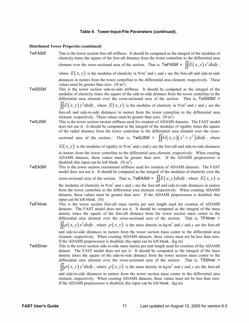
FAST User's Guide 71 Last updated on August 12, 2005 for version 6.0
Table 9. Tower-Input-File Parameters (continued).
Distributed Tower Properties (continued)
TwFAStif This is the tower section fore-aft stiffness. It should be computed as the integral of the modulus of elasticity times the square of the fore-aft distance from the tower centerline to the differential area
element over the cross-sectional area of the section. That is, TwFAStif = ( ) 2,∫∫ E x y x dxdy ,
where ( ),E x y is the modulus of elasticity in N/m2 and x and y are the fore-aft and side-to-side distances in meters from the tower centerline to the differential area element, respectively. These values must be greater than zero. (N·m2)
TwSSStif This is the tower section side-to-side stiffness. It should be computed as the integral of the modulus of elasticity times the square of the side-to-side distance from the tower centerline to the differential area element over the cross-sectional area of the section. That is, TwSSStif =
( ) 2,∫∫ E x y y dxdy , where ( ),E x y is the modulus of elasticity in N/m2 and x and y are the
fore-aft and side-to-side distances in meters from the tower centerline to the differential area element, respectively. These values must be greater than zero. (N·m2)
TwGJStif This is the tower section torsion stiffness used for creation of ADAMS datasets. The FAST model does not use it. It should be computed as the integral of the modulus of rigidity times the square of the radial distance from the tower centerline to the differential area element over the cross-sectional area of the section. That is, TwGJStif = ( )( )2 2, +∫∫G x y x y dxdy , where
( ),G x y is the modulus of rigidity in N/m2 and x and y are the fore-aft and side-to-side distances in meters from the tower centerline to the differential area element, respectively. When creating ADAMS datasets, these values must be greater than zero. If the ADAMS preprocessor is disabled, this input can be left blank. (N m2)
TwEAStif This is the tower section extensional stiffness used for creation of ADAMS datasets. The FAST model does not use it. It should be computed as the integral of the modulus of elasticity over the
cross-sectional area of the section. That is, TwEAStif = ( ),∫∫ E x y dxdy , where ( ),E x y is
the modulus of elasticity in N/m2 and x and y are the fore-aft and side-to-side distances in meters from the tower centerline to the differential area element, respectively. When creating ADAMS datasets, these values must be greater than zero. If the ADAMS preprocessor is disabled, this input can be left blank. (N)
TwFAIner This is the tower section fore-aft mass inertia per unit length used for creation of ADAMS datasets. The FAST model does not use it. It should be computed as the integral of the mass density times the square of the fore-aft distance from the tower section mass center to the differential area element over the cross-sectional area of the section. That is, TFAIner =
( ) 2,ρ∫∫ x y x dxdy , where ( ),ρ x y is the mass density in kg/m3 and x and y are the fore-aft
and side-to-side distances in meters from the tower section mass center to the differential area element, respectively. When creating ADAMS datasets, these values must not be less than zero. If the ADAMS preprocessor is disabled, this input can be left blank. (kg m)
TwSSIner This is the tower section side-to-side mass inertia per unit length used for creation of the ADAMS dataset. The FAST model does not use it. It should be computed as the integral of the mass density times the square of the side-to-side distance from the tower section mass center to the differential area element over the cross-sectional area of the section. That is, TSSIner =
( ) 2,ρ∫∫ x y y dxdy , where ( ),ρ x y is the mass density in kg/m3 and x and y are the fore-aft
and side-to-side distances in meters from the tower section mass center to the differential area element, respectively. When creating ADAMS datasets, these values must not be less than zero. If the ADAMS preprocessor is disabled, this input can be left blank. (kg m)
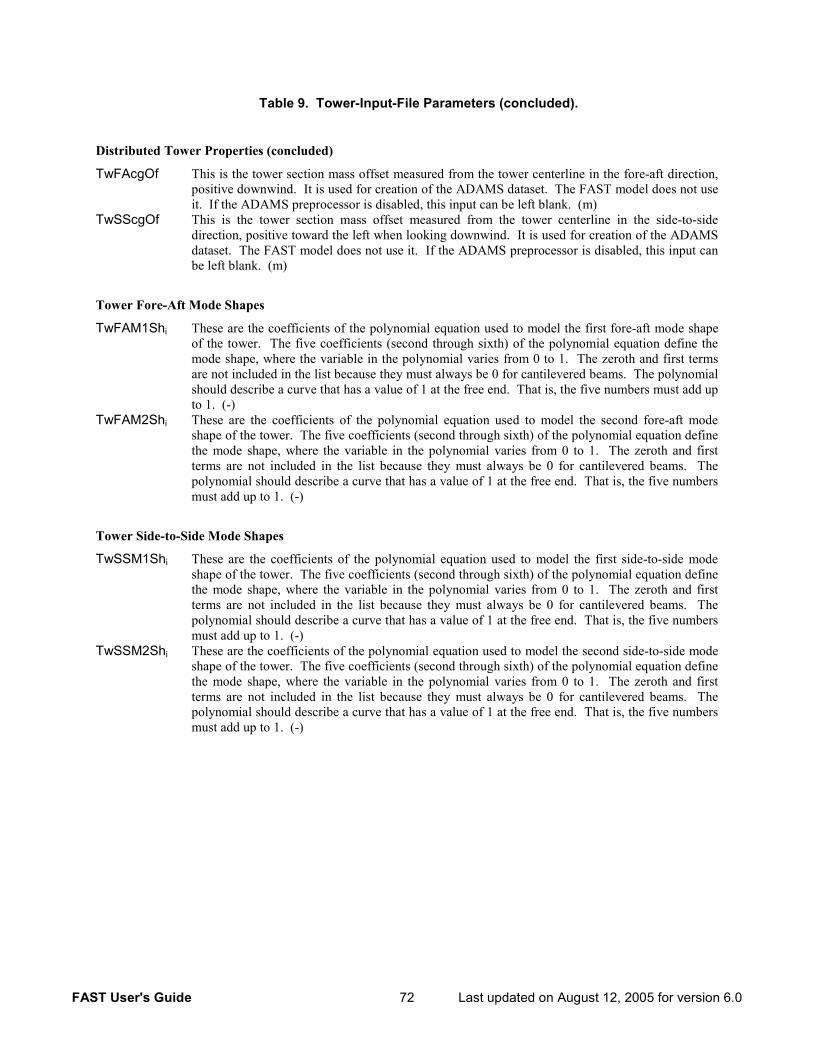
FAST User's Guide 72 Last updated on August 12, 2005 for version 6.0
Table 9. Tower-Input-File Parameters (concluded).
Distributed Tower Properties (concluded)
TwFAcgOf This is the tower section mass offset measured from the tower centerline in the fore-aft direction, positive downwind. It is used for creation of the ADAMS dataset. The FAST model does not use it. If the ADAMS preprocessor is disabled, this input can be left blank. (m)
TwSScgOf This is the tower section mass offset measured from the tower centerline in the side-to-side direction, positive toward the left when looking downwind. It is used for creation of the ADAMS dataset. The FAST model does not use it. If the ADAMS preprocessor is disabled, this input can be left blank. (m)
Tower Fore-Aft Mode Shapes
TwFAM1Shi These are the coefficients of the polynomial equation used to model the first fore-aft mode shape of the tower. The five coefficients (second through sixth) of the polynomial equation define the mode shape, where the variable in the polynomial varies from 0 to 1. The zeroth and first terms are not included in the list because they must always be 0 for cantilevered beams. The polynomial should describe a curve that has a value of 1 at the free end. That is, the five numbers must add up to 1. (-)
TwFAM2Shi These are the coefficients of the polynomial equation used to model the second fore-aft mode shape of the tower. The five coefficients (second through sixth) of the polynomial equation define the mode shape, where the variable in the polynomial varies from 0 to 1. The zeroth and first terms are not included in the list because they must always be 0 for cantilevered beams. The polynomial should describe a curve that has a value of 1 at the free end. That is, the five numbers must add up to 1. (-)
Tower Side-to-Side Mode Shapes
TwSSM1Shi These are the coefficients of the polynomial equation used to model the first side-to-side mode shape of the tower. The five coefficients (second through sixth) of the polynomial equation define the mode shape, where the variable in the polynomial varies from 0 to 1. The zeroth and first terms are not included in the list because they must always be 0 for cantilevered beams. The polynomial should describe a curve that has a value of 1 at the free end. That is, the five numbers must add up to 1. (-)
TwSSM2Shi These are the coefficients of the polynomial equation used to model the second side-to-side mode shape of the tower. The five coefficients (second through sixth) of the polynomial equation define the mode shape, where the variable in the polynomial varies from 0 to 1. The zeroth and first terms are not included in the list because they must always be 0 for cantilevered beams. The polynomial should describe a curve that has a value of 1 at the free end. That is, the five numbers must add up to 1. (-)
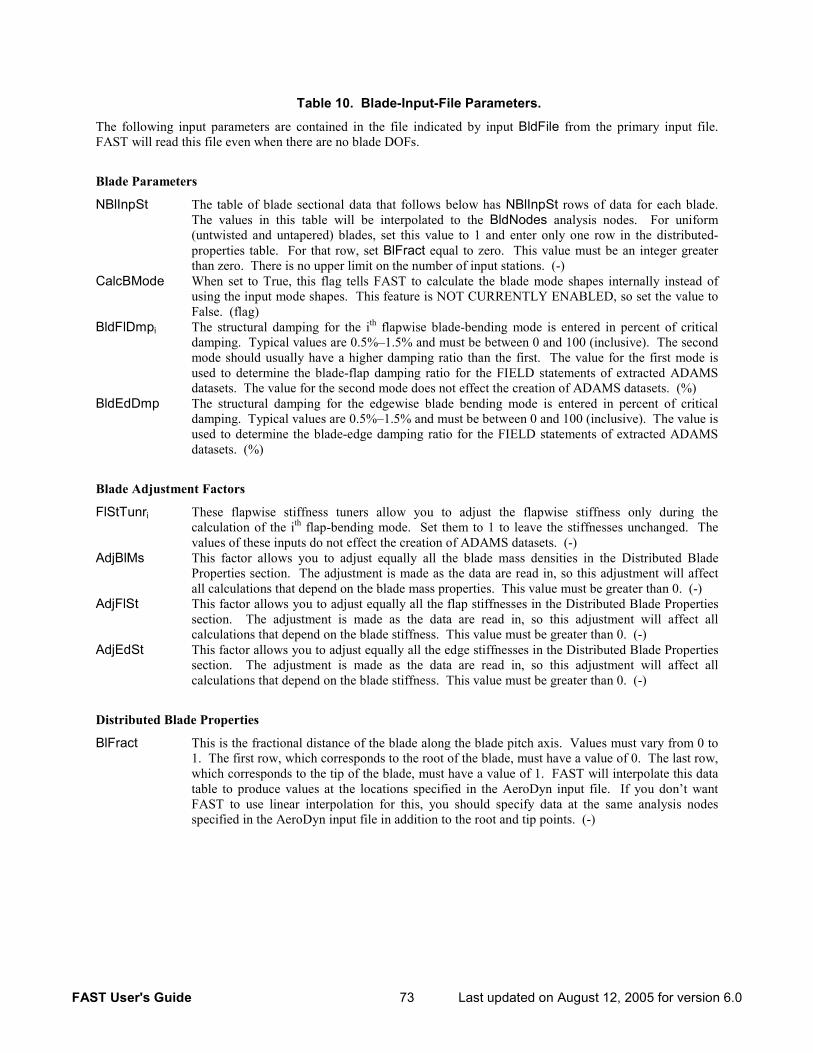
FAST User's Guide 73 Last updated on August 12, 2005 for version 6.0
Table 10. Blade-Input-File Parameters.
The following input parameters are contained in the file indicated by input BldFile from the primary input file. FAST will read this file even when there are no blade DOFs.
Blade Parameters
NBlInpSt The table of blade sectional data that follows below has NBlInpSt rows of data for each blade. The values in this table will be interpolated to the BldNodes analysis nodes. For uniform (untwisted and untapered) blades, set this value to 1 and enter only one row in the distributed-properties table. For that row, set BlFract equal to zero. This value must be an integer greater than zero. There is no upper limit on the number of input stations. (-)
CalcBMode When set to True, this flag tells FAST to calculate the blade mode shapes internally instead of using the input mode shapes. This feature is NOT CURRENTLY ENABLED, so set the value to False. (flag)
BldFlDmpi The structural damping for the ith flapwise blade-bending mode is entered in percent of critical damping. Typical values are 0.5%–1.5% and must be between 0 and 100 (inclusive). The second mode should usually have a higher damping ratio than the first. The value for the first mode is used to determine the blade-flap damping ratio for the FIELD statements of extracted ADAMS datasets. The value for the second mode does not effect the creation of ADAMS datasets. (%)
BldEdDmp The structural damping for the edgewise blade bending mode is entered in percent of critical damping. Typical values are 0.5%–1.5% and must be between 0 and 100 (inclusive). The value is used to determine the blade-edge damping ratio for the FIELD statements of extracted ADAMS datasets. (%)
Blade Adjustment Factors
FlStTunri These flapwise stiffness tuners allow you to adjust the flapwise stiffness only during the calculation of the ith flap-bending mode. Set them to 1 to leave the stiffnesses unchanged. The values of these inputs do not effect the creation of ADAMS datasets. (-)
AdjBlMs This factor allows you to adjust equally all the blade mass densities in the Distributed Blade Properties section. The adjustment is made as the data are read in, so this adjustment will affect all calculations that depend on the blade mass properties. This value must be greater than 0. (-)
AdjFlSt This factor allows you to adjust equally all the flap stiffnesses in the Distributed Blade Properties section. The adjustment is made as the data are read in, so this adjustment will affect all calculations that depend on the blade stiffness. This value must be greater than 0. (-)
AdjEdSt This factor allows you to adjust equally all the edge stiffnesses in the Distributed Blade Properties section. The adjustment is made as the data are read in, so this adjustment will affect all calculations that depend on the blade stiffness. This value must be greater than 0. (-)
Distributed Blade Properties
BlFract This is the fractional distance of the blade along the blade pitch axis. Values must vary from 0 to 1. The first row, which corresponds to the root of the blade, must have a value of 0. The last row, which corresponds to the tip of the blade, must have a value of 1. FAST will interpolate this data table to produce values at the locations specified in the AeroDyn input file. If you don’t want FAST to use linear interpolation for this, you should specify data at the same analysis nodes specified in the AeroDyn input file in addition to the root and tip points. (-)
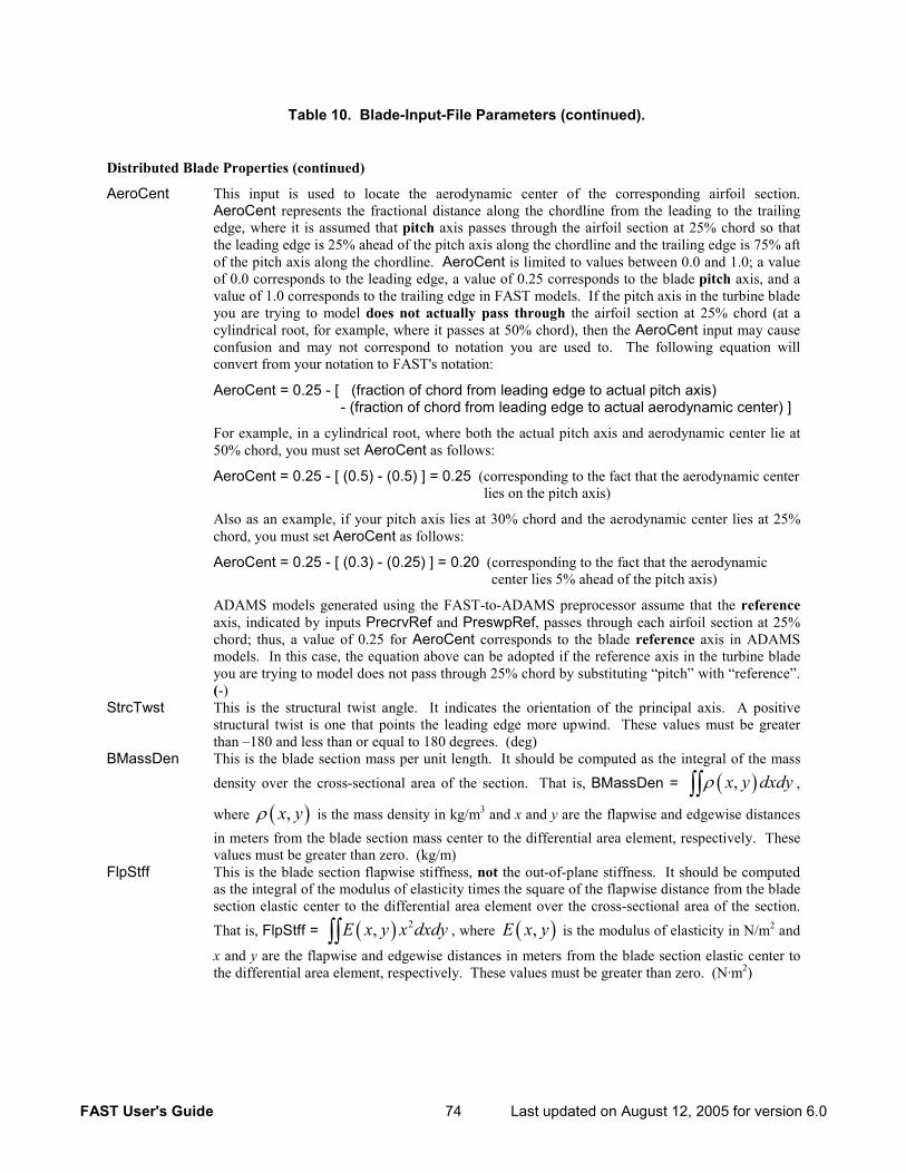
FAST User's Guide 74 Last updated on August 12, 2005 for version 6.0
Table 10. Blade-Input-File Parameters (continued).
Distributed Blade Properties (continued)
AeroCent This input is used to locate the aerodynamic center of the corresponding airfoil section. AeroCent represents the fractional distance along the chordline from the leading to the trailing edge, where it is assumed that pitch axis passes through the airfoil section at 25% chord so that the leading edge is 25% ahead of the pitch axis along the chordline and the trailing edge is 75% aft of the pitch axis along the chordline. AeroCent is limited to values between 0.0 and 1.0; a value of 0.0 corresponds to the leading edge, a value of 0.25 corresponds to the blade pitch axis, and a value of 1.0 corresponds to the trailing edge in FAST models. If the pitch axis in the turbine blade you are trying to model does not actually pass through the airfoil section at 25% chord (at a cylindrical root, for example, where it passes at 50% chord), then the AeroCent input may cause confusion and may not correspond to notation you are used to. The following equation will convert from your notation to FAST's notation:
AeroCent = 0.25 - [ (fraction of chord from leading edge to actual pitch axis) - (fraction of chord from leading edge to actual aerodynamic center) ]
For example, in a cylindrical root, where both the actual pitch axis and aerodynamic center lie at 50% chord, you must set AeroCent as follows:
AeroCent = 0.25 - [ (0.5) - (0.5) ] = 0.25 (corresponding to the fact that the aerodynamic center lies on the pitch axis)
Also as an example, if your pitch axis lies at 30% chord and the aerodynamic center lies at 25% chord, you must set AeroCent as follows:
AeroCent = 0.25 - [ (0.3) - (0.25) ] = 0.20 (corresponding to the fact that the aerodynamic center lies 5% ahead of the pitch axis)
ADAMS models generated using the FAST-to-ADAMS preprocessor assume that the reference axis, indicated by inputs PrecrvRef and PreswpRef, passes through each airfoil section at 25% chord; thus, a value of 0.25 for AeroCent corresponds to the blade reference axis in ADAMS models. In this case, the equation above can be adopted if the reference axis in the turbine blade you are trying to model does not pass through 25% chord by substituting “pitch” with “reference”. (-)
StrcTwst This is the structural twist angle. It indicates the orientation of the principal axis. A positive structural twist is one that points the leading edge more upwind. These values must be greater than –180 and less than or equal to 180 degrees. (deg)
BMassDen This is the blade section mass per unit length. It should be computed as the integral of the mass
density over the cross-sectional area of the section. That is, BMassDen = ( ),ρ∫∫ x y dxdy ,
where ( ),ρ x y is the mass density in kg/m3 and x and y are the flapwise and edgewise distances in meters from the blade section mass center to the differential area element, respectively. These values must be greater than zero. (kg/m)
FlpStff This is the blade section flapwise stiffness, not the out-of-plane stiffness. It should be computed as the integral of the modulus of elasticity times the square of the flapwise distance from the blade section elastic center to the differential area element over the cross-sectional area of the section.
That is, FlpStff = ( ) 2,∫∫ E x y x dxdy , where ( ),E x y is the modulus of elasticity in N/m2 and
x and y are the flapwise and edgewise distances in meters from the blade section elastic center to the differential area element, respectively. These values must be greater than zero. (N·m2)
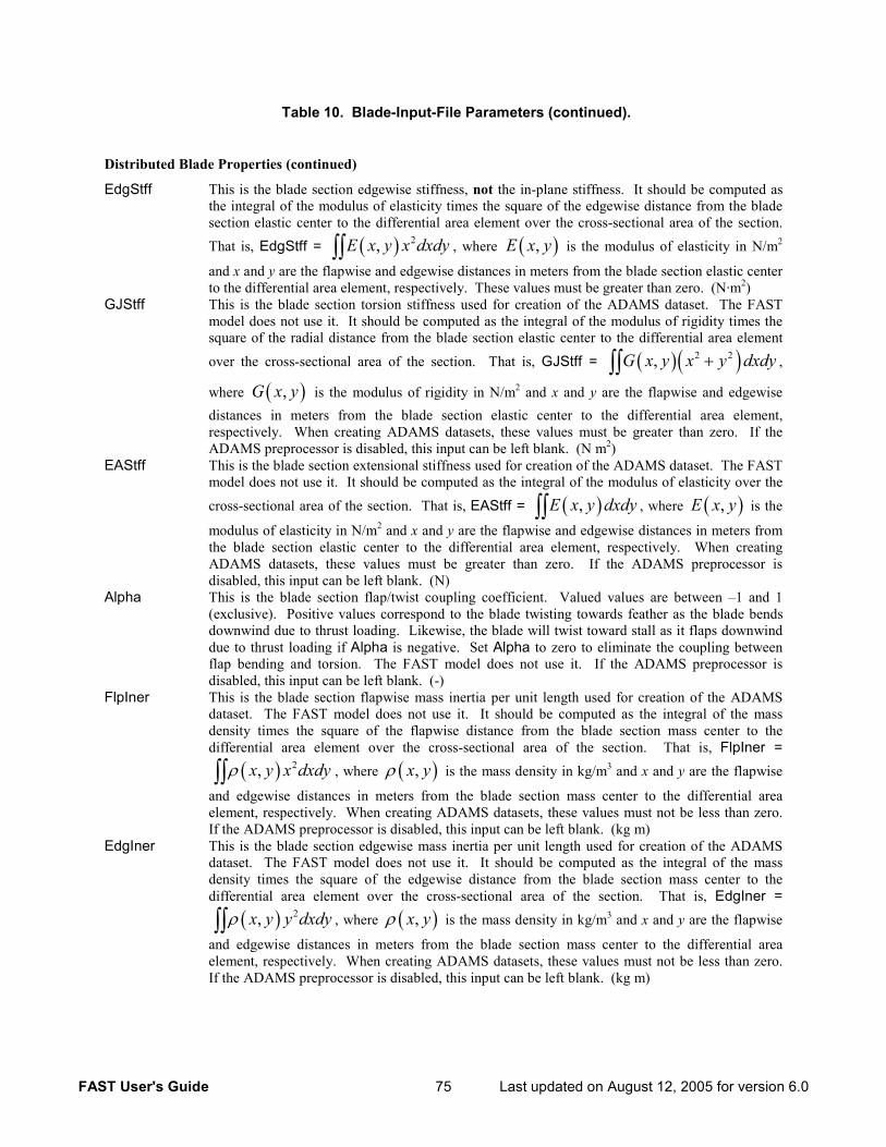
FAST User's Guide 75 Last updated on August 12, 2005 for version 6.0
Table 10. Blade-Input-File Parameters (continued).
Distributed Blade Properties (continued)
EdgStff This is the blade section edgewise stiffness, not the in-plane stiffness. It should be computed as the integral of the modulus of elasticity times the square of the edgewise distance from the blade section elastic center to the differential area element over the cross-sectional area of the section. That is, EdgStff = ( ) 2,∫∫ E x y x dxdy , where ( ),E x y is the modulus of elasticity in N/m2
and x and y are the flapwise and edgewise distances in meters from the blade section elastic center to the differential area element, respectively. These values must be greater than zero. (N·m2)
GJStff This is the blade section torsion stiffness used for creation of the ADAMS dataset. The FAST model does not use it. It should be computed as the integral of the modulus of rigidity times the square of the radial distance from the blade section elastic center to the differential area element
over the cross-sectional area of the section. That is, GJStff = ( )( )2 2, +∫∫G x y x y dxdy ,
where ( ),G x y is the modulus of rigidity in N/m2 and x and y are the flapwise and edgewise distances in meters from the blade section elastic center to the differential area element, respectively. When creating ADAMS datasets, these values must be greater than zero. If the ADAMS preprocessor is disabled, this input can be left blank. (N m2)
EAStff This is the blade section extensional stiffness used for creation of the ADAMS dataset. The FAST model does not use it. It should be computed as the integral of the modulus of elasticity over the
cross-sectional area of the section. That is, EAStff = ( ),E x y dxdy∫∫ , where ( ),E x y is the
modulus of elasticity in N/m2 and x and y are the flapwise and edgewise distances in meters from the blade section elastic center to the differential area element, respectively. When creating ADAMS datasets, these values must be greater than zero. If the ADAMS preprocessor is disabled, this input can be left blank. (N)
Alpha This is the blade section flap/twist coupling coefficient. Valued values are between –1 and 1 (exclusive). Positive values correspond to the blade twisting towards feather as the blade bends downwind due to thrust loading. Likewise, the blade will twist toward stall as it flaps downwind due to thrust loading if Alpha is negative. Set Alpha to zero to eliminate the coupling between flap bending and torsion. The FAST model does not use it. If the ADAMS preprocessor is disabled, this input can be left blank. (-)
FlpIner This is the blade section flapwise mass inertia per unit length used for creation of the ADAMS dataset. The FAST model does not use it. It should be computed as the integral of the mass density times the square of the flapwise distance from the blade section mass center to the differential area element over the cross-sectional area of the section. That is, FlpIner =
( ) 2,ρ∫∫ x y x dxdy , where ( ),ρ x y is the mass density in kg/m3 and x and y are the flapwise
and edgewise distances in meters from the blade section mass center to the differential area element, respectively. When creating ADAMS datasets, these values must not be less than zero. If the ADAMS preprocessor is disabled, this input can be left blank. (kg m)
EdgIner This is the blade section edgewise mass inertia per unit length used for creation of the ADAMS dataset. The FAST model does not use it. It should be computed as the integral of the mass density times the square of the edgewise distance from the blade section mass center to the differential area element over the cross-sectional area of the section. That is, EdgIner =
( ) 2,x y y dxdyρ∫∫ , where ( ),ρ x y is the mass density in kg/m3 and x and y are the flapwise
and edgewise distances in meters from the blade section mass center to the differential area element, respectively. When creating ADAMS datasets, these values must not be less than zero. If the ADAMS preprocessor is disabled, this input can be left blank. (kg m)
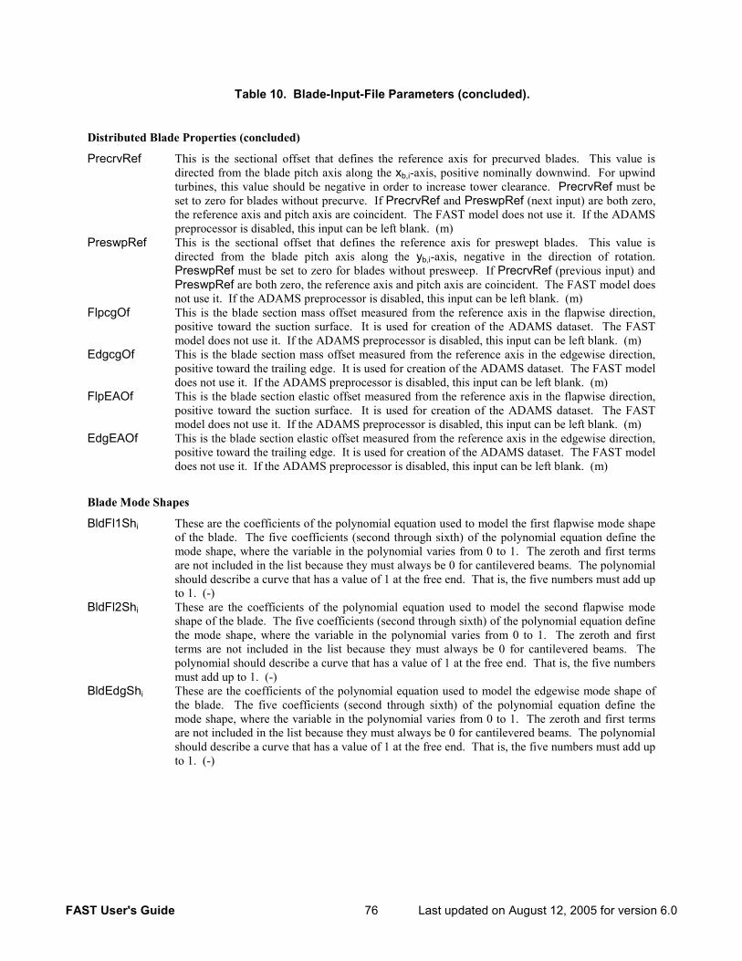
FAST User's Guide 76 Last updated on August 12, 2005 for version 6.0
Table 10. Blade-Input-File Parameters (concluded).
Distributed Blade Properties (concluded)
PrecrvRef This is the sectional offset that defines the reference axis for precurved blades. This value is directed from the blade pitch axis along the xb,i-axis, positive nominally downwind. For upwind turbines, this value should be negative in order to increase tower clearance. PrecrvRef must be set to zero for blades without precurve. If PrecrvRef and PreswpRef (next input) are both zero, the reference axis and pitch axis are coincident. The FAST model does not use it. If the ADAMS preprocessor is disabled, this input can be left blank. (m)
PreswpRef This is the sectional offset that defines the reference axis for preswept blades. This value is directed from the blade pitch axis along the yb,i-axis, negative in the direction of rotation. PreswpRef must be set to zero for blades without presweep. If PrecrvRef (previous input) and PreswpRef are both zero, the reference axis and pitch axis are coincident. The FAST model does not use it. If the ADAMS preprocessor is disabled, this input can be left blank. (m)
FlpcgOf This is the blade section mass offset measured from the reference axis in the flapwise direction, positive toward the suction surface. It is used for creation of the ADAMS dataset. The FAST model does not use it. If the ADAMS preprocessor is disabled, this input can be left blank. (m)
EdgcgOf This is the blade section mass offset measured from the reference axis in the edgewise direction, positive toward the trailing edge. It is used for creation of the ADAMS dataset. The FAST model does not use it. If the ADAMS preprocessor is disabled, this input can be left blank. (m)
FlpEAOf This is the blade section elastic offset measured from the reference axis in the flapwise direction, positive toward the suction surface. It is used for creation of the ADAMS dataset. The FAST model does not use it. If the ADAMS preprocessor is disabled, this input can be left blank. (m)
EdgEAOf This is the blade section elastic offset measured from the reference axis in the edgewise direction, positive toward the trailing edge. It is used for creation of the ADAMS dataset. The FAST model does not use it. If the ADAMS preprocessor is disabled, this input can be left blank. (m)
Blade Mode Shapes
BldFl1Shi These are the coefficients of the polynomial equation used to model the first flapwise mode shape of the blade. The five coefficients (second through sixth) of the polynomial equation define the mode shape, where the variable in the polynomial varies from 0 to 1. The zeroth and first terms are not included in the list because they must always be 0 for cantilevered beams. The polynomial should describe a curve that has a value of 1 at the free end. That is, the five numbers must add up to 1. (-)
BldFl2Shi These are the coefficients of the polynomial equation used to model the second flapwise mode shape of the blade. The five coefficients (second through sixth) of the polynomial equation define the mode shape, where the variable in the polynomial varies from 0 to 1. The zeroth and first terms are not included in the list because they must always be 0 for cantilevered beams. The polynomial should describe a curve that has a value of 1 at the free end. That is, the five numbers must add up to 1. (-)
BldEdgShi These are the coefficients of the polynomial equation used to model the edgewise mode shape of the blade. The five coefficients (second through sixth) of the polynomial equation define the mode shape, where the variable in the polynomial varies from 0 to 1. The zeroth and first terms are not included in the list because they must always be 0 for cantilevered beams. The polynomial should describe a curve that has a value of 1 at the free end. That is, the five numbers must add up to 1. (-)
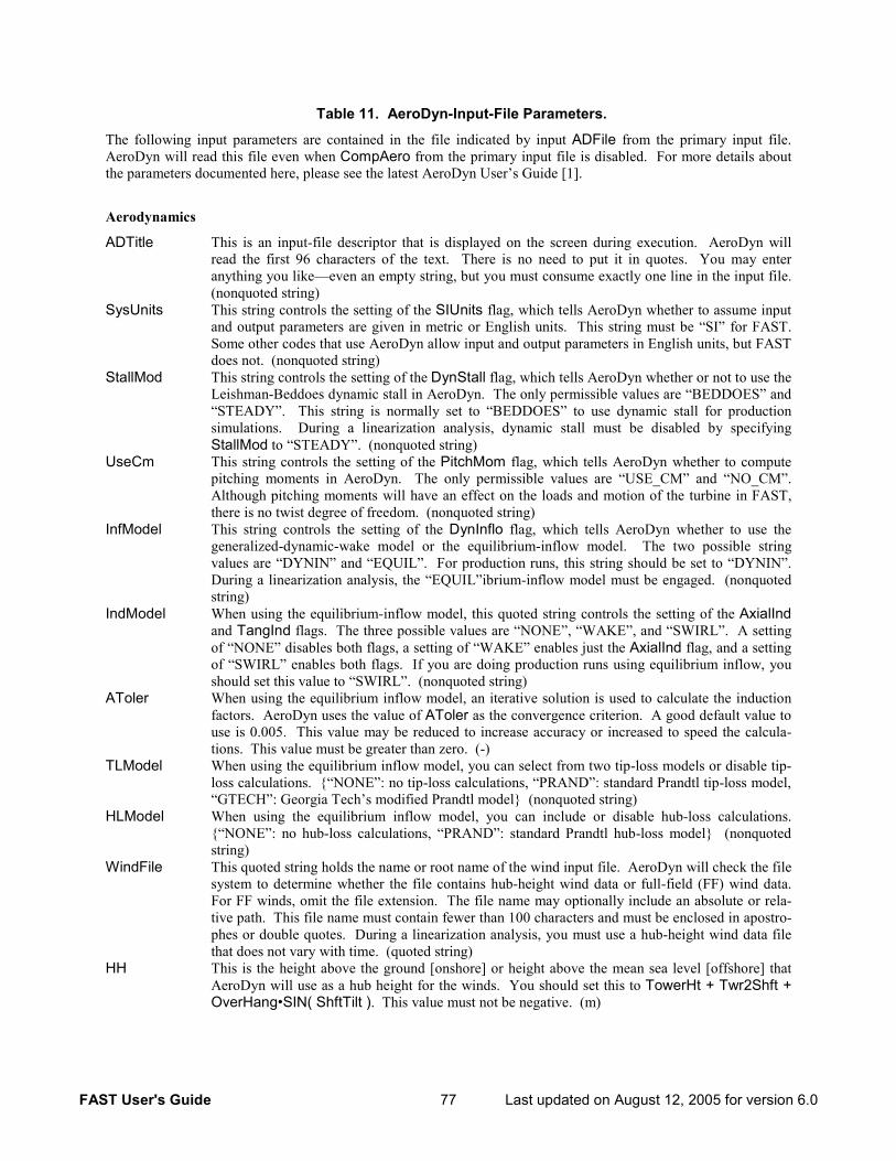
FAST User's Guide 77 Last updated on August 12, 2005 for version 6.0
Table 11. AeroDyn-Input-File Parameters.
The following input parameters are contained in the file indicated by input ADFile from the primary input file. AeroDyn will read this file even when CompAero from the primary input file is disabled. For more details about the parameters documented here, please see the latest AeroDyn User’s Guide [1].
Aerodynamics
ADTitle This is an input-file descriptor that is displayed on the screen during execution. AeroDyn will read the first 96 characters of the text. There is no need to put it in quotes. You may enter anything you like—even an empty string, but you must consume exactly one line in the input file. (nonquoted string)
SysUnits This string controls the setting of the SIUnits flag, which tells AeroDyn whether to assume input and output parameters are given in metric or English units. This string must be “SI” for FAST. Some other codes that use AeroDyn allow input and output parameters in English units, but FAST does not. (nonquoted string)
StallMod This string controls the setting of the DynStall flag, which tells AeroDyn whether or not to use the Leishman-Beddoes dynamic stall in AeroDyn. The only permissible values are “BEDDOES” and “STEADY”. This string is normally set to “BEDDOES” to use dynamic stall for production simulations. During a linearization analysis, dynamic stall must be disabled by specifying StallMod to “STEADY”. (nonquoted string)
UseCm This string controls the setting of the PitchMom flag, which tells AeroDyn whether to compute pitching moments in AeroDyn. The only permissible values are “USE_CM” and “NO_CM”. Although pitching moments will have an effect on the loads and motion of the turbine in FAST, there is no twist degree of freedom. (nonquoted string)
InfModel This string controls the setting of the DynInflo flag, which tells AeroDyn whether to use the generalized-dynamic-wake model or the equilibrium-inflow model. The two possible string values are “DYNIN” and “EQUIL”. For production runs, this string should be set to “DYNIN”. During a linearization analysis, the “EQUIL”ibrium-inflow model must be engaged. (nonquoted string)
IndModel When using the equilibrium-inflow model, this quoted string controls the setting of the AxialInd and TangInd flags. The three possible values are “NONE”, “WAKE”, and “SWIRL”. A setting of “NONE” disables both flags, a setting of “WAKE” enables just the AxialInd flag, and a setting of “SWIRL” enables both flags. If you are doing production runs using equilibrium inflow, you should set this value to “SWIRL”. (nonquoted string)
AToler When using the equilibrium inflow model, an iterative solution is used to calculate the induction factors. AeroDyn uses the value of AToler as the convergence criterion. A good default value to use is 0.005. This value may be reduced to increase accuracy or increased to speed the calcula-tions. This value must be greater than zero. (-)
TLModel When using the equilibrium inflow model, you can select from two tip-loss models or disable tip-loss calculations. “NONE”: no tip-loss calculations, “PRAND”: standard Prandtl tip-loss model, “GTECH”: Georgia Tech’s modified Prandtl model (nonquoted string)
HLModel When using the equilibrium inflow model, you can include or disable hub-loss calculations. “NONE”: no hub-loss calculations, “PRAND”: standard Prandtl hub-loss model (nonquoted string)
WindFile This quoted string holds the name or root name of the wind input file. AeroDyn will check the file system to determine whether the file contains hub-height wind data or full-field (FF) wind data. For FF winds, omit the file extension. The file name may optionally include an absolute or rela-tive path. This file name must contain fewer than 100 characters and must be enclosed in apostro-phes or double quotes. During a linearization analysis, you must use a hub-height wind data file that does not vary with time. (quoted string)
HH This is the height above the ground [onshore] or height above the mean sea level [offshore] that AeroDyn will use as a hub height for the winds. You should set this to TowerHt + Twr2Shft + OverHang•SIN( ShftTilt ). This value must not be negative. (m)
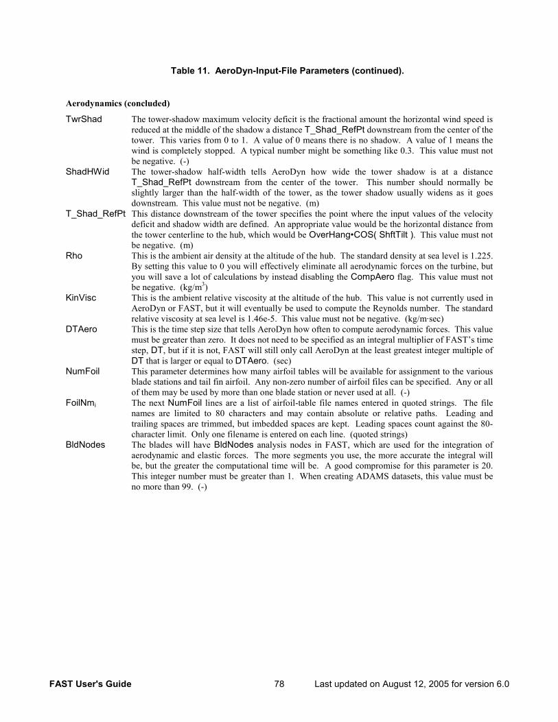
FAST User's Guide 78 Last updated on August 12, 2005 for version 6.0
Table 11. AeroDyn-Input-File Parameters (continued).
Aerodynamics (concluded)
TwrShad The tower-shadow maximum velocity deficit is the fractional amount the horizontal wind speed is reduced at the middle of the shadow a distance T_Shad_RefPt downstream from the center of the tower. This varies from 0 to 1. A value of 0 means there is no shadow. A value of 1 means the wind is completely stopped. A typical number might be something like 0.3. This value must not be negative. (-)
ShadHWid The tower-shadow half-width tells AeroDyn how wide the tower shadow is at a distance T_Shad_RefPt downstream from the center of the tower. This number should normally be slightly larger than the half-width of the tower, as the tower shadow usually widens as it goes downstream. This value must not be negative. (m)
T_Shad_RefPt This distance downstream of the tower specifies the point where the input values of the velocity deficit and shadow width are defined. An appropriate value would be the horizontal distance from the tower centerline to the hub, which would be OverHang•COS( ShftTilt ). This value must not be negative. (m)
Rho This is the ambient air density at the altitude of the hub. The standard density at sea level is 1.225. By setting this value to 0 you will effectively eliminate all aerodynamic forces on the turbine, but you will save a lot of calculations by instead disabling the CompAero flag. This value must not be negative. (kg/m3)
KinVisc This is the ambient relative viscosity at the altitude of the hub. This value is not currently used in AeroDyn or FAST, but it will eventually be used to compute the Reynolds number. The standard relative viscosity at sea level is 1.46e-5. This value must not be negative. (kg/m·sec)
DTAero This is the time step size that tells AeroDyn how often to compute aerodynamic forces. This value must be greater than zero. It does not need to be specified as an integral multiplier of FAST’s time step, DT, but if it is not, FAST will still only call AeroDyn at the least greatest integer multiple of DT that is larger or equal to DTAero. (sec)
NumFoil This parameter determines how many airfoil tables will be available for assignment to the various blade stations and tail fin airfoil. Any non-zero number of airfoil files can be specified. Any or all of them may be used by more than one blade station or never used at all. (-)
FoilNmi The next NumFoil lines are a list of airfoil-table file names entered in quoted strings. The file names are limited to 80 characters and may contain absolute or relative paths. Leading and trailing spaces are trimmed, but imbedded spaces are kept. Leading spaces count against the 80-character limit. Only one filename is entered on each line. (quoted strings)
BldNodes The blades will have BldNodes analysis nodes in FAST, which are used for the integration of aerodynamic and elastic forces. The more segments you use, the more accurate the integral will be, but the greater the computational time will be. A good compromise for this parameter is 20. This integer number must be greater than 1. When creating ADAMS datasets, this value must be no more than 99. (-)
FAST User's Guide 79 Last updated on August 12, 2005 for version 6.0
Table 11. AeroDyn-Input-File Parameters (concluded).
Distributed Blade Information
RNodes These values are the distances of the analysis nodes from the rotor apex along the pitch axis, which is not consistent with the YawDyn convention for 3-bladed turbines (but is consistent for 2-bladed turbines). The analysis nodes are located at the centers of the blade segments. You do not have complete freedom to put the RNodes anywhere you like. For instance, they cannot be at the blade root or tip. It is also not always possible to alternate between nodes that are close together and far apart. An easy way to ensure consistency is to divide the blade segments and then compute the centers of the segments to use for the RNodes. The nodes do not need to be equally spaced. These values must fall between the HubRad and TipRad (exclusive). (m)
AeroTwst This is the aerodynamic twist angle. It indicates the orientation of the chord of the local airfoil. A positive aerodynamic twist is one that points the leading edge more upwind. These values must be greater than –180 and less than or equal to 180 degrees. (deg)
DRNodes These values represent the portion of the blade span that is assigned to an analysis node. This length times the local chord defines the area used in the aerodynamics calculations. The sum of all the DRNodes should add up to the blade length. FAST checks the values of the RNodes and DRNodes to make sure they are consistent and meaningful. These values must be greater than zero. (m)
Chord These values are the local chords of the analysis nodes. This local chord times DRNodes defines the area used in the aerodynamics calculations. These values must be greater than zero. (m)
NFoil These integers tell AeroDyn which of the input airfoil files (FoilNm) are assigned to the various analysis nodes. For instance, a value of 2 means that node 2 will use FoilNm2 for the local airfoil. Airfoils may be assigned to more than one blade station. These values must be between 1 and NumFoil. (-)
PrnElm If the whole word “PRINT” is found anywhere on a line, the element data for that element will be printed to the element output file (element.plt). You can also enter the nonquoted string “NOPRINT”, or leave this field blank to skip printing element data for this element. (nonquoted, case-insensitive string)

FAST User's Guide 80 Last updated on August 12, 2005 for version 6.0
Table 12. Platform-Input-File Parameters.
The following input parameters are contained in the file indicated by input PtfmFile from the primary input file. FAST will only read this file if PtfmModel from the primary input file is nonzero. In FAST v6.0, all nonzero PtfmModel options will work the same way by reading in the PtfmFile described here. In future versions, the format of this file will depend on which PtfmModel option is selected.
Feature Flags
PtfmSgDOF The support platform surge DOF will be enabled when this is True. The surge DOF allows the platform to translate horizontally relative to the inertia frame as shown in Figure 20. The platform reference point (located by input PtfmRef) translates with the platform during this motion. The initial surge displacement is specified with PtfmSurge. If PtfmSgDOF is disabled, the surge displacement will be fixed at PtfmSurge. (flag)
PtfmSwDOF The support platform sway DOF will be enabled when this is True. The sway DOF allows the platform to translate horizontally relative to the inertia frame as shown in Figure 20. The platform reference point (located by input PtfmRef) translates with the platform during this motion. The initial sway displacement is specified with PtfmSway. If PtfmSwDOF is disabled, the sway displacement will be fixed at PtfmSway. (flag)
PtfmHvDOF The support platform heave DOF will be enabled when this is True. The heave DOF allows the platform to translate vertically relative to the inertia frame as shown in Figure 20. The platform reference point (located by input PtfmRef) translates with the platform during this motion. The initial heave displacement is specified with PtfmHeave. If PtfmHvDOF is disabled, the heave displacement will be fixed at PtfmHeave. (flag)
PtfmRDOF The support platform roll DOF will be enabled when this is True. The roll DOF allows the platform to tilt (rotate) about its reference point (located by input PtfmRef) relative to the inertia frame as shown in Figure 20. The initial roll displacement is specified with PtfmRoll. If PtfmRDOF is disabled, the roll displacement will be fixed at PtfmRoll. (flag)
PtfmPDOF The support platform pitch DOF will be enabled when this is True. The pitch DOF allows the platform to tilt (rotate) about its reference point (located by input PtfmRef) relative to the inertia frame as shown in Figure 20. The initial pitch displacement is specified with PtfmPitch. If PtfmPDOF is disabled, the pitch displacement will be fixed at PtfmPitch. (flag)
PtfmYDOF The support platform yaw DOF will be enabled when this is True. The yaw DOF allows the platform to yaw (rotate) about its reference point (located by input PtfmRef) relative to the inertia frame as shown in Figure 20. The initial yaw displacement is specified with PtfmYaw. If PtfmYDOF is disabled, the yaw displacement will be fixed at PtfmYaw. (flag)
Initial Conditions
PtfmSurge This is the fixed or initial support platform surge displacement. The surge displacement indicates a horizontal translation of the platform relative to the inertia frame as shown in Figure 20. (m)
PtfmSway This is the fixed or initial support platform sway displacement. The sway displacement indicates a horizontal translation of the platform relative to the inertia frame as shown in Figure 20. (m)
PtfmHeave This is the fixed or initial support platform heave displacement. The heave displacement indicates a vertical translation of the platform relative to the inertia frame as shown in Figure 20. (m)
PtfmRoll This is the fixed or initial support platform roll displacement. The roll displacement indicates a tilt rotation of the platform about its reference point (located by input PtfmRef) relative to the inertia frame as shown in Figure 20. This value must be between –15 and 15 degrees (inclusive). (deg)
PtfmPitch This is the fixed or initial support platform pitch displacement. The pitch displacement indicates a tilt rotation of the platform about its reference point (located by input PtfmRef) relative to the inertia frame as shown in Figure 20. This value must be between –15 and 15 degrees (inclusive). (deg)
PtfmYaw This is the fixed or initial support platform yaw displacement. The yaw displacement indicates a yaw rotation of the platform about its reference point (located by input PtfmRef) relative to the inertia frame as shown in Figure 20. This value must be between –15 and 15 degrees (inclusive). (deg)
FAST User's Guide 81 Last updated on August 12, 2005 for version 6.0
Table 12. Platform-Input-File Parameters (concluded).
Turbine Configuration
TwrDraft The tower draft is the downward distance from ground level [onshore] or mean sea level [offshore] to the tower base platform connection. This value must be greater than –TowerHt. See Figure 20. (m)
PtfmCM This is the downward distance from ground level [onshore] or mean sea level [offshore] to the support platform mass center. This value must not be less than TwrDraft. See Figure 20. (m)
PtfmRef This is the downward distance from ground level [onshore] or mean sea level [offshore] to the support platform reference point. The platform reference point is the origin in the platform about which the translational (surge, sway, and heave) and rotational (roll, pitch, and yaw) motions of the support platform are defined. It is also the point at which external loading is applied to the platform—see input parameter PtfmLdMod. This value must not be less than TwrDraft. See Figure 20. (m)
Mass and Inertia
PtfmMass This is the mass of the support platform. Its center is located a downward distance of PtfmCM from ground level [onshore] or mean sea level [offshore]. If TwrRBHt is nonzero, the mass of the rigid portion of the tower should be included with the support platform mass in PtfmMass. This value must not be negative. (kg)
PtfmRIner This is the support platform moment of inertia in roll about the platform mass center. It includes all mass contained in PtfmMass. This value must not be negative. (kg·m2)
PtfmPIner This is the support platform moment of inertia in pitch about the platform mass center. It includes all mass contained in PtfmMass. This value must not be negative. (kg·m2)
PtfmYIner This is the support platform moment of inertia in yaw about the platform mass center. It includes all mass contained in PtfmMass. This value must not be negative. (kg·m2)
Platform Loading
PtfmLdMod In FAST v6.0, only user-defined platform loading is available. For a value of 0 for PtfmLdMod, there will be no platform loading and the support reactions normally produced will be set to zero (causing the wind turbine to fall due to gravity if PtfmHvDOF is True). If you set PtfmLdMod to 1, FAST will call the routine UserPtfmLd() to compute the platform loading. You should replace the dummy routine supplied with the code with your own, which will need to be linked with the rest of FAST. The platform loads returned by UserPtfmLd() should contain contributions from any external load acting on the platform other than loads transmitted from the wind turbine. For example, these loads should contain contributions from foundation stiffness and damping [not floating] or mooring line restoring and damping [floating], as well as hydrostatic and hydrodynamic contributions [offshore]. The platform loads will be applied on the platform at the instantaneous platform reference position (located by input PtfmRef). The routine assumes that the platform loads are transmitted through a medium like soil [foundation] and/or water [offshore], so that added mass effects are important. See the dummy UserPtfmLd() routine for more information. Using values other than 0 or 1 for PtfmLdMod will cause FAST to abort. (switch)
FAST User's Guide 82 Last updated on August 12, 2005 for version 6.0
Table 13. Furling-Input-File Parameters.
The following input parameters are contained in the file indicated by input FurlFile from the primary input file. FAST will only read this file if the model is designated as a furling machine (when Furling from the primary input file is set to True).
Feature Flags
RFrlDOF The rotor-furl DOF will be enabled when this is True. The initial rotor-furl angle is specified with RotFurl. If RFrlDOF is disabled, the rotor-furl angle will be fixed at RotFurl. (flag)
TFrlDOF The tail-furl DOF will be enabled when this is True. The initial tail-furl angle is specified with TailFurl. If TFrlDOF is disabled, the tail-furl angle will be fixed at TailFurl. (flag)
Initial Conditions
RotFurl This is the fixed or initial rotor-furl angle. It is positive about the rotor-furl axis as shown in Figure 17. The rotor-furl axis is defined through inputs RFrlPntxn, RFrlPntyn, RFrlPntzn, RFrlSkew, and RFrlTilt below. This value must be greater than –180 and less than or equal to 180 degrees. (deg)
TailFurl This is the fixed or initial tail-furl angle. It is positive about the tail-furl axis as shown in Figure 17. The tail-furl axis is defined through inputs TFrlPntxn, TFrlPntyn, TFrlPntzn, TFrlSkew, and TFrlTilt below. This value must be greater than –180 and less than or equal to 180 degrees. (deg)
Turbine Configuration
Yaw2Shft This is the lateral offset distance from the yaw axis to the intersection of the rotor shaft axis with the yn-/zn-plane. The distance is measured parallel to the yn-axis. It is positive to the left when looking downwind as shown in Figure 18. For turbines with rotor-furl, this distance defines the configuration at a furl angle of zero. (m)
ShftSkew This is the skew angle of the rotor shaft in the nominally horizontal plane. Positive skew acts like positive nacelle yaw as shown in Figure 18; however, ShftSkew should only be used to skew the shaft a few degrees away from the zero-yaw position and must not be used as a replacement for the yaw angle. This value must be between –15 and 15 degrees (inclusive). For turbines with rotor-furl, this angle defines the configuration at a furl angle of zero. (deg)
RFrlCMxn This is the downwind distance to the center of mass of the structure that furls with the rotor (not including the rotor—reference input RFrlMass) from the top of the tower, measured parallel to the xn-axis. It is positive downwind. See Figure 18. For turbines with rotor-furl, this distance defines the configuration at a furl angle of zero. (m)
RFrlCMyn This is the lateral distance to the center of mass of the structure that furls with the rotor (not including the rotor—reference input RFrlMass) from the top of the tower, measured parallel to the yn-axis. It is positive to the left when looking downwind. See Figure 18. For turbines with rotor-furl, this distance defines the configuration at a furl angle of zero. (m)
RFrlCMzn This is the vertical distance to the center of mass of the structure that furls with the rotor (not including the rotor—reference input RFrlMass) from the top of the tower, measured parallel to the zn-axis. It is positive upward when looking downwind. See Figure 18. For turbines with rotor-furl, this distance defines the configuration at a furl angle of zero. (m)
BoomCMxn This is the downwind distance to the tail boom mass center (reference input BoomMass) from the top of the tower, measured parallel to the xn-axis. It is positive downwind. See Figure 19. For turbines with tail-furl, this distance defines the configuration at a furl angle of zero. (m)
BoomCMyn This is the lateral distance to the tail boom mass center (reference input BoomMass) from the top of the tower, measured parallel to the yn-axis. It is positive to the left when looking downwind. See Figure 19. For turbines with tail-furl, this distance defines the configuration at a furl angle of zero. (m)
BoomCMzn This is the vertical distance to the tail boom mass center (reference input BoomMass) from the top of the tower, measured parallel to the zn-axis. It is positive upward when looking downwind. See Figure 19. For turbines with tail-furl, this distance defines the configuration at a furl angle of zero. (m)
FAST User's Guide 83 Last updated on August 12, 2005 for version 6.0
Table 13. Furling-Input-File Parameters (continued).
Turbine Configuration (continued)
TFinCMxn This is the downwind distance to the tail fin mass center (reference input TFinMass) from the top of the tower, measured parallel to the xn-axis. It is positive downwind. See Figure 19. For turbines with tail-furl, this distance defines the configuration at a furl angle of zero. (m)
TFinCMyn This is the lateral distance to the tail fin mass center (reference input TFinMass) from the top of the tower, measured parallel to the yn-axis. It is positive to the left when looking downwind. See Figure 19. For turbines with tail-furl, this distance defines the configuration at a furl angle of zero. (m)
TFinCMzn This is the vertical distance to the tail fin mass center (reference input TFinMass) from the top of the tower, measured parallel to the zn-axis. It is positive upward when looking downwind. See Figure 19. For turbines with tail-furl, this distance defines the configuration at a furl angle of zero. (m)
TFinCPxn This is the downwind distance to the tail fin center-of-pressure from the top of the tower, measured parallel to the xn-axis. It is positive downwind. See Figure 19. For turbines with tail-furl, this distance defines the configuration at a furl angle of zero. (m)
TFinCPyn This is the lateral distance to the tail fin center-of-pressure from the top of the tower, measured parallel to the yn-axis. It is positive to the left when looking downwind. See Figure 19. For turbines with tail-furl, this distance defines the configuration at a furl angle of zero. (m)
TFinCPzn This is the vertical distance to the tail fin center-of-pressure from the top of the tower, measured parallel to the zn-axis. It is positive upward when looking downwind. See Figure 19. For turbines with tail-furl, this distance defines the configuration at a furl angle of zero. (m)
TFinSkew This is the skew angle of the tail fin chordline in the nominally horizontal plane. Positive skew orients the nominal horizontal projection of the tail fin chordline about the zn-axis. The aforementioned chordline is the chordline passing through the tail fin center-of-pressure. See Figure 19. This value must be greater than –180 and less than or equal to 180 degrees. For turbines with tail-furl, this angle defines the configuration at a furl angle of zero. (deg)
TFinTilt This is the tilt angle of the tail fin chordline from the nominally horizontal plane. The aforementioned chordline is the chordline passing through the tail fin center-of-pressure. This value must be between –90 and 90 degrees (inclusive). Positive tilt means that the trailing edge of the tail fin is higher than the leading edge. See Figure 19. For turbines with tail-furl, this angle defines the configuration at a furl angle of zero. (deg)
TFinBank This is the bank angle of the tail fin plane about the tail fin chordline. The aforementioned chordline is the chordline passing through the tail fin center-of-pressure. This value must be greater than –180 and less than or equal to 180 degrees. See Figure 19. For turbines with tail-furl, this angle defines the configuration at a furl angle of zero. (deg)
RFrlPntxn This is the downwind distance to an arbitrary point on the rotor-furl axis from the top of the tower, measured parallel to the xn-axis. It is positive downwind. The arbitrary point referred to in this input must be the same point identified by inputs RFrlPntyn and RFrlPntzn. Inputs RFrlPntxn, RFrlPntyn, RFrlPntzn, RFrlSkew, and RFrlTilt define the orientation of the rotor-furl axis and associated DOF, RFrlDOF. See Figure 17. (m)
RFrlPntyn This is the lateral distance to an arbitrary point on the rotor-furl axis from the top of the tower, measured parallel to the yn-axis. It is positive to the left when looking downwind. The arbitrary point referred to in this input must be the same point identified by inputs RFrlPntxn and RFrlPntzn. Inputs RFrlPntxn, RFrlPntyn, RFrlPntzn, RFrlSkew, and RFrlTilt define the orientation of the rotor-furl axis and associated DOF, RFrlDOF. See Figure 17. (m)
RFrlPntzn This is the vertical distance to an arbitrary point on the rotor-furl axis from the top of the tower, measured parallel to the zn-axis. It is positive upward when looking downwind. The arbitrary point referred to in this input must be the same point identified by inputs RFrlPntxn and RFrlPntyn. Inputs RFrlPntxn, RFrlPntyn, RFrlPntzn, RFrlSkew, and RFrlTilt define the orientation of the rotor-furl axis and associated DOF, RFrlDOF. See Figure 17. (m)
FAST User's Guide 84 Last updated on August 12, 2005 for version 6.0
Table 13. Furling-Input-File Parameters (continued).
Turbine Configuration (concluded)
RFrlSkew This is the skew angle of the rotor-furl axis in the nominally horizontal plane. Positive skew orients the nominal horizontal projection of the rotor-furl axis about the zn-axis. Inputs RFrlPntxn, RFrlPntyn, RFrlPntzn, RFrlSkew, and RFrlTilt define the orientation of the rotor-furl axis and associated DOF, RFrlDOF. See Figure 17. This value must be greater than –180 and less than or equal to 180 degrees. (deg)
RFrlTilt This is the tilt angle of the rotor-furl axis from the nominally horizontal plane. This value must be between –90 and 90 degrees (inclusive). Inputs RFrlPntxn, RFrlPntyn, RFrlPntzn, RFrlSkew, and RFrlTilt define the orientation of the rotor-furl axis and associated DOF, RFrlDOF. See Figure 17. (deg)
TFrlPntxn This is the downwind distance to an arbitrary point on the tail-furl axis from the top of the tower, measured parallel to the xn-axis. It is positive downwind. The arbitrary point referred to in this input must be the same point identified by inputs TFrlPntyn and TFrlPntzn. Inputs TFrlPntxn, TFrlPntyn, TFrlPntzn, TFrlSkew, and TFrlTilt define the orientation of the tail-furl axis and associated DOF, TFrlDOF. See Figure 17. (m)
TFrlPntyn This is the lateral distance to an arbitrary point on the tail-furl axis from the top of the tower, measured parallel to the yn-axis. It is positive to the left when looking downwind. The arbitrary point referred to in this input must be the same point identified by inputs TFrlPntxn and TFrlPntzn. Inputs TFrlPntxn, TFrlPntyn, TFrlPntzn, TFrlSkew, and TFrlTilt define the orientation of the tail-furl axis and associated DOF, TFrlDOF. See Figure 17. (m)
TFrlPntzn This is the vertical distance to an arbitrary point on the tail-furl axis from the top of the tower, measured parallel to the zn-axis. It is positive upward when looking downwind. The arbitrary point referred to in this input must be the same point identified by inputs TFrlPntxn and TFrlPntyn. Inputs TFrlPntxn, TFrlPntyn, TFrlPntzn, TFrlSkew, and TFrlTilt define the orientation of the tail-furl axis and associated DOF, RFrlDOF. See Figure 17. (m)
TFrlSkew This is the skew angle of the tail-furl axis in the nominally horizontal plane. Positive skew orients the nominal horizontal projection of the tail-furl axis about the zn-axis. Inputs TFrlPntxn, TFrlPntyn, TFrlPntzn, TFrlSkew, and TFrlTilt define the orientation of the tail-furl axis and associated DOF, TFrlDOF. See Figure 17. This value must be greater than –180 and less than or equal to 180 degrees. (deg)
TFrlTilt This is the tilt angle of the tail-furl axis from the nominally horizontal plane. This value must be between –90 and 90 degrees (inclusive). Inputs TFrlPntxn, TFrlPntyn, TFrlPntzn, TFrlSkew, and TFrlTilt define the orientation of the tail-furl axis and associated DOF, TFrlDOF. See Figure 17. (deg)
Mass and Inertia
RFrlMass This is the mass of the structure that furls with the rotor (not including the rotor). The center of this mass is located at the point specified by inputs RFrlCMxn, RFrlCMyn, and RFrlCMzn relative to the tower-top at a rotor-furl angle of zero. It includes everything that furls with the rotor excluding the rotor (blades, hub, and tip brakes). This value must not be negative. (kg)
BoomMass This is the mass of the tail boom. The center of the tail boom mass is located at the point specified by inputs BoomCMxn, BoomCMyn, and BoomCMzn relative to the tower-top at a tail-furl angle of zero. It includes everything that furls with the tail except the tail fin (see next input). This value must not be negative. (kg)
TFinMass This is the mass of the tail fin. The center of the tail fin mass is located at the point specified by inputs TFinCMxn, TFinCMyn, and TFinCMzn relative to the tower-top at a tail-furl angle of zero. TFinMass and BoomMass combined should include everything that furls with the tail. This value must not be negative. (kg)
RFrlIner This is the moment of inertia of the structure that furls with the rotor (not including the rotor) about the rotor-furl axis. It includes all mass contained in RFrlMass. This value must be greater than RFrlMass•( perpendicular distance between rotor-furl axis and C.M. of the structure that furls with the rotor [not including the rotor] )2. (kg·m2)
FAST User's Guide 85 Last updated on August 12, 2005 for version 6.0
Table 13. Furling-Input-File Parameters (continued).
Mass and Inertia (concluded)
TFrlIner This is the tail boom moment of inertia about the tail-furl axis. It includes all mass contained in BoomMass. This value must be greater than BoomMass•( perpendicular distance between tail-furl axis and tail boom C.M. )2. (kg·m2)
Rotor-Furl
RFrlMod The rotor-furl springs and dampers can be modeled three ways. For a value of 0 for RFrlMod, there will be no rotor-furl spring nor damper and the moment normally produced will be set to zero. A RFrlMod of 1 will invoke simple spring and damper models using the inputs provided below as appropriate coefficients. If you set RFrlMod to 2, FAST will call the routine UserRFrl() to compute the rotor-furl spring and damper moments. You should replace the dummy routine supplied with the code with your own, which will need to be linked with the rest of FAST. Using values other than 0, 1, or 2 will cause FAST to abort. (switch)
RFrlSpr The linear rotor-furl spring restoring moment is proportional to the rotor-furl deflection through this constant. This value must not be negative and is only used when RFrlMod is set to 1. (N·m/rad)
RFrlDmp The linear rotor-furl damping moment is proportional to the rotor-furl rate through this constant. This value must not be negative and is only used when RFrlMod is set to 1. (N·m/(rad/sec))
RFrlCDmp This Coulomb-friction damping moment resists rotor-furl motion, but it is a constant that is not proportional to the rotor-furl rate. However, if the rotor-furl rate is zero, the damping is zero. This value must not be negative and is only used when RFrlMod is set to 1. (N·m)
RFrlUSSP The rotor-furl up-stop spring is effective when the rotor-furl deflection exceeds this value. This value must be greater than –180 and less than or equal to 180 degrees and is only used when RFrlMod is set to 1. (deg)
RFrlDSSP The rotor-furl down-stop spring is effective when the rotor-furl deflection exceeds this value. This value must be greater than –180 and less than or equal to RFrlUSSP degrees and is only used when RFrlMod is set to 1. (deg)
RFrlUSSpr The linear rotor-furl up-stop spring restoring moment is proportional to the rotor-furl up-stop deflection by this constant and is effective when the rotor-furl deflection exceeds RFrlUSSP. This value must not be negative and is only used when RFrlMod is set to 1. (N·m/rad)
RFrlDSSpr The linear rotor-furl down-stop spring restoring moment is proportional to the rotor-furl down-stop deflection by this constant and is effective when the rotor-furl deflection exceeds RFrlDSSP. This value must not be negative and is only used when RFrlMod is set to 1. (N·m/rad)
RFrlUSDP The rotor-furl up-stop damper is effective when the rotor-furl deflection exceeds this value. This value must be greater than –180 and less than or equal to 180 degrees and is only used when RFrlMod is set to 1. (deg)
RFrlDSDP The rotor-furl down-stop damper is effective when the rotor-furl deflection exceeds this value. This value must be greater than –180 and less than or equal to RFrlUSDP degrees and is only used when RFrlMod is set to 1. (deg)
RFrlUSDmp The linear rotor-furl up-stop damping moment is proportional to the rotor-furl rate by this constant and is effective when the rotor-furl deflection exceeds RFrlUSDP. This value must not be negative and is only used when RFrlMod is set to 1. (N·m/(rad/sec))
RFrlDSDmp The linear rotor-furl down-stop damping restoring moment is proportional to the rotor-furl rate by this constant and is effective when the rotor-furl deflection exceeds RFrlDSDP. This value must not be negative and is only used when RFrlMod is set to 1. (N·m/(rad/sec))
FAST User's Guide 86 Last updated on August 12, 2005 for version 6.0
Table 13. Furling-Input-File Parameters (continued).
Tail-Furl
TFrlMod The tail-furl springs and dampers can be modeled three ways. For a value of 0 for TFrlMod, there will be no tail-furl spring nor damper and the moment normally produced will be set to zero. A TFrlMod of 1 will invoke simple spring and damper models using the inputs provided below as appropriate coefficients. If you set TFrlMod to 2, FAST will call the routine UserTFrl() to compute the tail-furl spring and damper moments. You should replace the dummy routine supplied with the code with your own, which will need to be linked with the rest of FAST. Using values other than 0, 1, or 2 will cause FAST to abort. (switch)
TFrlSpr The linear tail-furl spring restoring moment is proportional to the tail-furl deflection through this constant. This value must not be negative and is only used when TFrlMod is set to 1. (N·m/rad)
TFrlDmp The linear tail-furl damping moment is proportional to the tail-furl rate through this constant. This value must not be negative and is only used when TFrlMod is set to 1. (N·m/(rad/sec))
TFrlCDmp This Coulomb-friction damping moment resists tail-furl motion, but it is a constant that is not proportional to the tail-furl rate. However, if the tail-furl rate is zero, the damping is zero. This value must not be negative and is only used when TFrlMod is set to 1. (N·m)
TFrlUSSP The tail-furl up-stop spring is effective when the tail-furl deflection exceeds this value. This value must be greater than –180 and less than or equal to 180 degrees and is only used when TFrlMod is set to 1. (deg)
TFrlDSSP The tail-furl down-stop spring is effective when the tail-furl deflection exceeds this value. This value must be greater than –180 and less than or equal to TFrlUSSP degrees and is only used when TFrlMod is set to 1. (deg)
TFrlUSSpr The linear tail-furl up-stop spring restoring moment is proportional to the tail-furl up-stop deflection by this constant and is effective when the tail-furl deflection exceeds TFrlUSSP. This value must not be negative and is only used when TFrlMod is set to 1. (N·m/rad)
TFrlDSSpr The linear tail-furl down-stop spring restoring moment is proportional to the tail-furl down-stop deflection by this constant and is effective when the tail-furl deflection exceeds TFrlDSSP. This value must not be negative and is only used when TFrlMod is set to 1. (N·m/rad)
TFrlUSDP The tail-furl up-stop damper is effective when the tail-furl deflection exceeds this value. This value must be greater than –180 and less than or equal to 180 degrees and is only used when TFrlMod is set to 1. (deg)
TFrlDSDP The tail-furl down-stop damper is effective when the tail-furl deflection exceeds this value. This value must be greater than –180 and less than or equal to TFrlUSDP degrees and is only used when TFrlMod is set to 1. (deg)
TFrlUSDmp The linear tail-furl up-stop damping moment is proportional to the tail-furl rate by this constant and is effective when the tail-furl deflection exceeds TFrlUSDP. This value must not be negative and is only used when TFrlMod is set to 1. (N·m/(rad/sec))
TFrlDSDmp The linear tail-furl down-stop damping restoring moment is proportional to the tail-furl rate by this constant and is effective when the tail-furl deflection exceeds TFrlDSDP. This value must not be negative and is only used when TFrlMod is set to 1. (N·m/(rad/sec))
FAST User's Guide 87 Last updated on August 12, 2005 for version 6.0
Table 13. Furling-Input-File Parameters (concluded).
Tail Fin Aerodynamics
TFinMod The tail fin aerodynamics can be modeled three ways. For a value of 0 for TFinMod, there will be no tail fin aerodynamics and the aerodynamic loads normally produced will be set to zero. A TFinMod of 1 will invoke a simplified tail fin aerodynamics model using the inputs provided below as appropriate parameters. If you set TFinMod to 2, FAST will call the routine UserTFin() to compute the tail fin aerodynamic loads. You should replace the dummy routine supplied with the code with your own, which will need to be linked with the rest of FAST. Using values other than 0, 1, or 2 will cause FAST to abort. (switch)
TFinNFoil This integer tells AeroDyn which of the input airfoil files (FoilNm) is assigned to the tail fin. For instance, a value of 2 means that the tail fin will use FoilNm2 for the local tail fin airfoil. The tail fin airfoil may be assigned to the same airfoil as one or more blade stations. This value must be between 1 and NumFoil and is only used when TFinMod is set to 1. (-)
TFinArea This is the plan form area of the tail fin plate used to relate the local dynamic pressure and airfoil coefficients to aerodynamic loads. This value must not be negative and is only used when TFinMod is set to 1. (m2)
SubAxInd Set this value to False if you want the wind velocity at the tail fin to be unobstructed by the rotor wake. Set this value to True if you want FAST to decrease (i.e., subtract) the wind velocity at the tail fin center-of-pressure in the rotor shaft direction by the average rotor axial induction. This input is only used when TFinMod is set to 1. (flag)
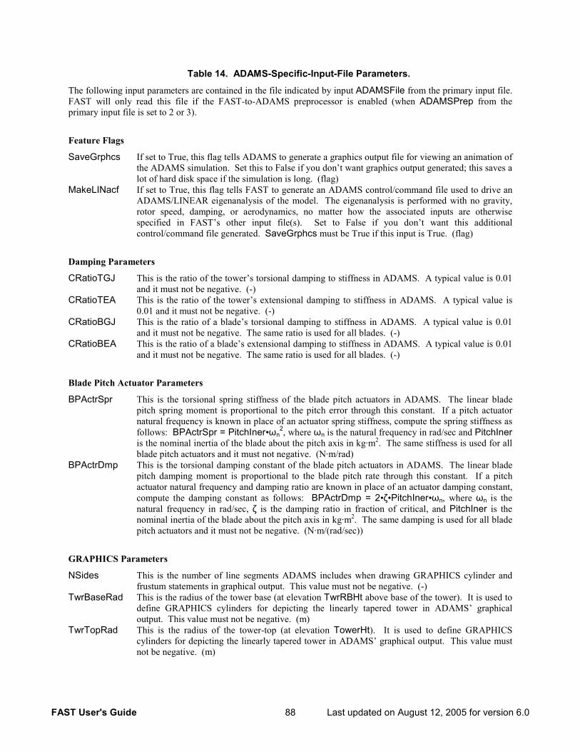
FAST User's Guide 88 Last updated on August 12, 2005 for version 6.0
Table 14. ADAMS-Specific-Input-File Parameters.
The following input parameters are contained in the file indicated by input ADAMSFile from the primary input file. FAST will only read this file if the FAST-to-ADAMS preprocessor is enabled (when ADAMSPrep from the primary input file is set to 2 or 3).
Feature Flags
SaveGrphcs If set to True, this flag tells ADAMS to generate a graphics output file for viewing an animation of the ADAMS simulation. Set this to False if you don’t want graphics output generated; this saves a lot of hard disk space if the simulation is long. (flag)
MakeLINacf If set to True, this flag tells FAST to generate an ADAMS control/command file used to drive an ADAMS/LINEAR eigenanalysis of the model. The eigenanalysis is performed with no gravity, rotor speed, damping, or aerodynamics, no matter how the associated inputs are otherwise specified in FAST’s other input file(s). Set to False if you don’t want this additional control/command file generated. SaveGrphcs must be True if this input is True. (flag)
Damping Parameters
CRatioTGJ This is the ratio of the tower’s torsional damping to stiffness in ADAMS. A typical value is 0.01 and it must not be negative. (-)
CRatioTEA This is the ratio of the tower’s extensional damping to stiffness in ADAMS. A typical value is 0.01 and it must not be negative. (-)
CRatioBGJ This is the ratio of a blade’s torsional damping to stiffness in ADAMS. A typical value is 0.01 and it must not be negative. The same ratio is used for all blades. (-)
CRatioBEA This is the ratio of a blade’s extensional damping to stiffness in ADAMS. A typical value is 0.01 and it must not be negative. The same ratio is used for all blades. (-)
Blade Pitch Actuator Parameters
BPActrSpr This is the torsional spring stiffness of the blade pitch actuators in ADAMS. The linear blade pitch spring moment is proportional to the pitch error through this constant. If a pitch actuator natural frequency is known in place of an actuator spring stiffness, compute the spring stiffness as follows: BPActrSpr = PitchIner•ωn
2, where ωn is the natural frequency in rad/sec and PitchIner is the nominal inertia of the blade about the pitch axis in kg·m2. The same stiffness is used for all blade pitch actuators and it must not negative. (N·m/rad)
BPActrDmp This is the torsional damping constant of the blade pitch actuators in ADAMS. The linear blade pitch damping moment is proportional to the blade pitch rate through this constant. If a pitch actuator natural frequency and damping ratio are known in place of an actuator damping constant, compute the damping constant as follows: BPActrDmp = 2•ζ•PitchIner•ωn, where ωn is the natural frequency in rad/sec, ζ is the damping ratio in fraction of critical, and PitchIner is the nominal inertia of the blade about the pitch axis in kg·m2. The same damping is used for all blade pitch actuators and it must not be negative. (N·m/(rad/sec))
GRAPHICS Parameters
NSides This is the number of line segments ADAMS includes when drawing GRAPHICS cylinder and frustum statements in graphical output. This value must not be negative. (-)
TwrBaseRad This is the radius of the tower base (at elevation TwrRBHt above base of the tower). It is used to define GRAPHICS cylinders for depicting the linearly tapered tower in ADAMS’ graphical output. This value must not be negative. (m)
TwrTopRad This is the radius of the tower-top (at elevation TowerHt). It is used to define GRAPHICS cylinders for depicting the linearly tapered tower in ADAMS’ graphical output. This value must not be negative. (m)
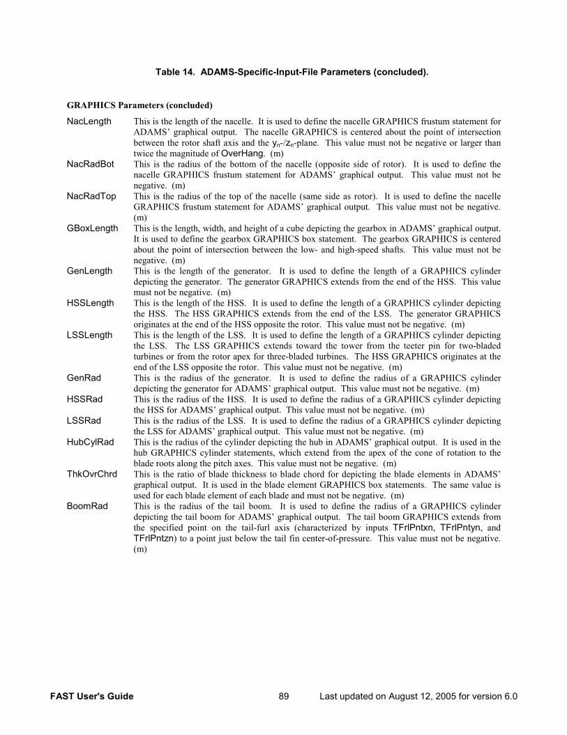
FAST User's Guide 89 Last updated on August 12, 2005 for version 6.0
Table 14. ADAMS-Specific-Input-File Parameters (concluded).
GRAPHICS Parameters (concluded)
NacLength This is the length of the nacelle. It is used to define the nacelle GRAPHICS frustum statement for ADAMS’ graphical output. The nacelle GRAPHICS is centered about the point of intersection between the rotor shaft axis and the yn-/zn-plane. This value must not be negative or larger than twice the magnitude of OverHang. (m)
NacRadBot This is the radius of the bottom of the nacelle (opposite side of rotor). It is used to define the nacelle GRAPHICS frustum statement for ADAMS’ graphical output. This value must not be negative. (m)
NacRadTop This is the radius of the top of the nacelle (same side as rotor). It is used to define the nacelle GRAPHICS frustum statement for ADAMS’ graphical output. This value must not be negative. (m)
GBoxLength This is the length, width, and height of a cube depicting the gearbox in ADAMS’ graphical output. It is used to define the gearbox GRAPHICS box statement. The gearbox GRAPHICS is centered about the point of intersection between the low- and high-speed shafts. This value must not be negative. (m)
GenLength This is the length of the generator. It is used to define the length of a GRAPHICS cylinder depicting the generator. The generator GRAPHICS extends from the end of the HSS. This value must not be negative. (m)
HSSLength This is the length of the HSS. It is used to define the length of a GRAPHICS cylinder depicting the HSS. The HSS GRAPHICS extends from the end of the LSS. The generator GRAPHICS originates at the end of the HSS opposite the rotor. This value must not be negative. (m)
LSSLength This is the length of the LSS. It is used to define the length of a GRAPHICS cylinder depicting the LSS. The LSS GRAPHICS extends toward the tower from the teeter pin for two-bladed turbines or from the rotor apex for three-bladed turbines. The HSS GRAPHICS originates at the end of the LSS opposite the rotor. This value must not be negative. (m)
GenRad This is the radius of the generator. It is used to define the radius of a GRAPHICS cylinder depicting the generator for ADAMS’ graphical output. This value must not be negative. (m)
HSSRad This is the radius of the HSS. It is used to define the radius of a GRAPHICS cylinder depicting the HSS for ADAMS’ graphical output. This value must not be negative. (m)
LSSRad This is the radius of the LSS. It is used to define the radius of a GRAPHICS cylinder depicting the LSS for ADAMS’ graphical output. This value must not be negative. (m)
HubCylRad This is the radius of the cylinder depicting the hub in ADAMS’ graphical output. It is used in the hub GRAPHICS cylinder statements, which extend from the apex of the cone of rotation to the blade roots along the pitch axes. This value must not be negative. (m)
ThkOvrChrd This is the ratio of blade thickness to blade chord for depicting the blade elements in ADAMS’ graphical output. It is used in the blade element GRAPHICS box statements. The same value is used for each blade element of each blade and must not be negative. (m)
BoomRad This is the radius of the tail boom. It is used to define the radius of a GRAPHICS cylinder depicting the tail boom for ADAMS’ graphical output. The tail boom GRAPHICS extends from the specified point on the tail-furl axis (characterized by inputs TFrlPntxn, TFrlPntyn, and TFrlPntzn) to a point just below the tail fin center-of-pressure. This value must not be negative. (m)
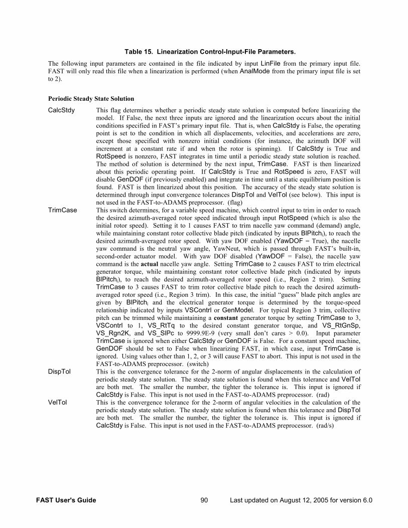
FAST User's Guide 90 Last updated on August 12, 2005 for version 6.0
Table 15. Linearization Control-Input-File Parameters.
The following input parameters are contained in the file indicated by input LinFile from the primary input file. FAST will only read this file when a linearization is performed (when AnalMode from the primary input file is set to 2).
Periodic Steady State Solution
CalcStdy This flag determines whether a periodic steady state solution is computed before linearizing the model. If False, the next three inputs are ignored and the linearization occurs about the initial conditions specified in FAST’s primary input file. That is, when CalcStdy is False, the operating point is set to the condition in which all displacements, velocities, and accelerations are zero, except those specified with nonzero initial conditions (for instance, the azimuth DOF will increment at a constant rate if and when the rotor is spinning). If CalcStdy is True and RotSpeed is nonzero, FAST integrates in time until a periodic steady state solution is reached. The method of solution is determined by the next input, TrimCase. FAST is then linearized about this periodic operating point. If CalcStdy is True and RotSpeed is zero, FAST will disable GenDOF (if previously enabled) and integrate in time until a static equilibrium position is found. FAST is then linearized about this position. The accuracy of the steady state solution is determined through input convergence tolerances DispTol and VelTol (see below). This input is not used in the FAST-to-ADAMS preprocessor. (flag)
TrimCase This switch determines, for a variable speed machine, which control input to trim in order to reach the desired azimuth-averaged rotor speed indicated through input RotSpeed (which is also the initial rotor speed). Setting it to 1 causes FAST to trim nacelle yaw command (demand) angle, while maintaining constant rotor collective blade pitch (indicated by inputs BlPitchi), to reach the desired azimuth-averaged rotor speed. With yaw DOF enabled (YawDOF = True), the nacelle yaw command is the neutral yaw angle, YawNeut, which is passed through FAST’s built-in, second-order actuator model. With yaw DOF disabled (YawDOF = False), the nacelle yaw command is the actual nacelle yaw angle. Setting TrimCase to 2 causes FAST to trim electrical generator torque, while maintaining constant rotor collective blade pitch (indicated by inputs BlPitchi), to reach the desired azimuth-averaged rotor speed (i.e., Region 2 trim). Setting TrimCase to 3 causes FAST to trim rotor collective blade pitch to reach the desired azimuth-averaged rotor speed (i.e., Region 3 trim). In this case, the initial “guess” blade pitch angles are given by BlPitchi and the electrical generator torque is determined by the torque-speed relationship indicated by inputs VSContrl or GenModel. For typical Region 3 trim, collective pitch can be trimmed while maintaining a constant generator torque by setting TrimCase to 3, VSContrl to 1, VS_RtTq to the desired constant generator torque, and VS_RtGnSp, VS_Rgn2K, and VS_SlPc to 9999.9E-9 (very small don’t cares > 0.0). Input parameter TrimCase is ignored when either CalcStdy or GenDOF is False. For a constant speed machine, GenDOF should be set to False when linearizing FAST, in which case, input TrimCase is ignored. Using values other than 1, 2, or 3 will cause FAST to abort. This input is not used in the FAST-to-ADAMS preprocessor. (switch)
DispTol This is the convergence tolerance for the 2-norm of angular displacements in the calculation of periodic steady state solution. The steady state solution is found when this tolerance and VelTol are both met. The smaller the number, the tighter the tolerance is. This input is ignored if CalcStdy is False. This input is not used in the FAST-to-ADAMS preprocessor. (rad)
VelTol This is the convergence tolerance for the 2-norm of angular velocities in the calculation of the periodic steady state solution. The steady state solution is found when this tolerance and DispTol are both met. The smaller the number, the tighter the tolerance is. This input is ignored if CalcStdy is False. This input is not used in the FAST-to-ADAMS preprocessor. (rad/s)
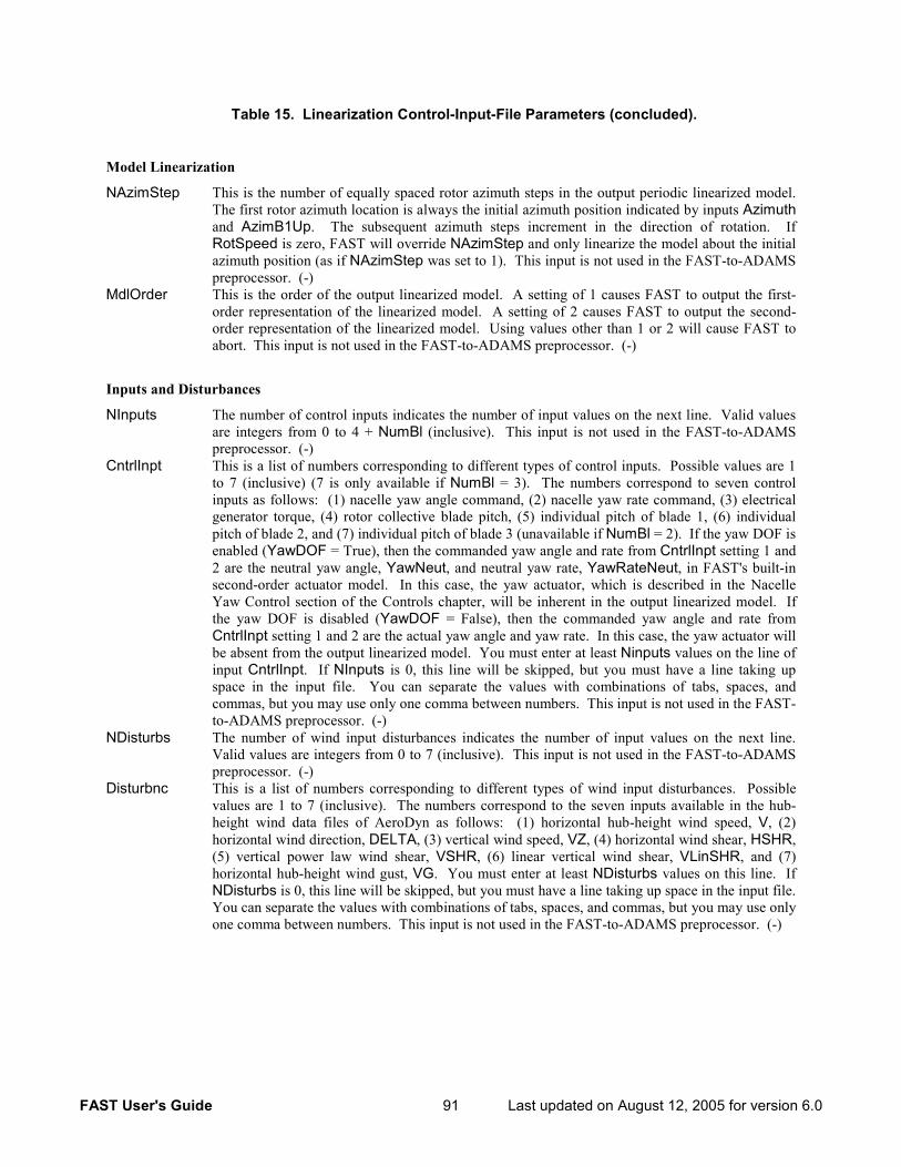
FAST User's Guide 91 Last updated on August 12, 2005 for version 6.0
Table 15. Linearization Control-Input-File Parameters (concluded).
Model Linearization
NAzimStep This is the number of equally spaced rotor azimuth steps in the output periodic linearized model. The first rotor azimuth location is always the initial azimuth position indicated by inputs Azimuth and AzimB1Up. The subsequent azimuth steps increment in the direction of rotation. If RotSpeed is zero, FAST will override NAzimStep and only linearize the model about the initial azimuth position (as if NAzimStep was set to 1). This input is not used in the FAST-to-ADAMS preprocessor. (-)
MdlOrder This is the order of the output linearized model. A setting of 1 causes FAST to output the first-order representation of the linearized model. A setting of 2 causes FAST to output the second-order representation of the linearized model. Using values other than 1 or 2 will cause FAST to abort. This input is not used in the FAST-to-ADAMS preprocessor. (-)
Inputs and Disturbances
NInputs The number of control inputs indicates the number of input values on the next line. Valid values are integers from 0 to 4 + NumBl (inclusive). This input is not used in the FAST-to-ADAMS preprocessor. (-)
CntrlInpt This is a list of numbers corresponding to different types of control inputs. Possible values are 1 to 7 (inclusive) (7 is only available if NumBl = 3). The numbers correspond to seven control inputs as follows: (1) nacelle yaw angle command, (2) nacelle yaw rate command, (3) electrical generator torque, (4) rotor collective blade pitch, (5) individual pitch of blade 1, (6) individual pitch of blade 2, and (7) individual pitch of blade 3 (unavailable if NumBl = 2). If the yaw DOF is enabled (YawDOF = True), then the commanded yaw angle and rate from CntrlInpt setting 1 and 2 are the neutral yaw angle, YawNeut, and neutral yaw rate, YawRateNeut, in FAST's built-in second-order actuator model. In this case, the yaw actuator, which is described in the Nacelle Yaw Control section of the Controls chapter, will be inherent in the output linearized model. If the yaw DOF is disabled (YawDOF = False), then the commanded yaw angle and rate from CntrlInpt setting 1 and 2 are the actual yaw angle and yaw rate. In this case, the yaw actuator will be absent from the output linearized model. You must enter at least Ninputs values on the line of input CntrlInpt. If NInputs is 0, this line will be skipped, but you must have a line taking up space in the input file. You can separate the values with combinations of tabs, spaces, and commas, but you may use only one comma between numbers. This input is not used in the FAST-to-ADAMS preprocessor. (-)
NDisturbs The number of wind input disturbances indicates the number of input values on the next line. Valid values are integers from 0 to 7 (inclusive). This input is not used in the FAST-to-ADAMS preprocessor. (-)
Disturbnc This is a list of numbers corresponding to different types of wind input disturbances. Possible values are 1 to 7 (inclusive). The numbers correspond to the seven inputs available in the hub-height wind data files of AeroDyn as follows: (1) horizontal hub-height wind speed, V, (2) horizontal wind direction, DELTA, (3) vertical wind speed, VZ, (4) horizontal wind shear, HSHR, (5) vertical power law wind shear, VSHR, (6) linear vertical wind shear, VLinSHR, and (7) horizontal hub-height wind gust, VG. You must enter at least NDisturbs values on this line. If NDisturbs is 0, this line will be skipped, but you must have a line taking up space in the input file. You can separate the values with combinations of tabs, spaces, and commas, but you may use only one comma between numbers. This input is not used in the FAST-to-ADAMS preprocessor. (-)

FAST User's Guide 93 Last updated on August 12, 2005 for version 6.0
OUTPUT FILES
The program generates one or more output files based on settings in the input file.
For time-marching analyses, the primary output file contains columns of time-series data with one column for each parameter that is requested in the primary input file. The name of this file uses the path and root name of the primary input file and appends .out for an extension. For example, if the input file were named fast.fst, the main output file will be named fast.out. The available output parameters are shown in Table 16 through Table 44 and are also documented in the OutList.txt file of the FAST archive. An example output file is shown in Figure 30.
In some situations, some output channels are meaningless. For instance, if aerodynamic calculations are disabled, parameters such as the wind speed are invalid. You can still leave those parameters in your output list, but the data generated will be all zeros. The name and units for the channel will also be replaced with “INVALID” and “CHANNEL” respectively. Output loads and motions follow the IEC system. Please refer to Figure 3 through Figure 9 to get a sense for which directions are positive.
For linearization analyses, the primary output file provides the periodic state matrices of the linearized model. The name of this file uses the path and root name of the primary input file and appends .lin for an extension. For example, if the input file were named fast.fst, the main output file will be named fast.lin. An example linearized model file is shown in Figure 31.
If the SumPrint flag is set to True, FAST generates a second output file, with a .fsm for an extension. In the above example, this file will be
named fast.fsm. This file contains some of the basic input file parameters and computed inertia properties of the blades and tower. An example summary file is shown in Figure 32.
If the SumPrint flag is set to True, AeroDyn also generates a summary file that contains blade-element geometry data, airfoil data files at the corresponding blade element, and the summary of combined FAST/AeroDyn input parameters. In the above example, this file will be named fast.opt. An example of this AeroDyn output can be found in Figure 33.
If ADAMSPrep is set to 2 or 3, FAST generates ADAMS dataset files corresponding to the model configuration and analysis settings specified in the FAST input file(s). See the ADAMS Preprocessor chapter for a description of these output files.
A final file is generated only when the word “PRINT” is found on one or more of the lines defining the blade elements in the AeroDyn input file. This file contains a time series of aerodynamic data and has a .elm extension, as in, fast.elm. Please see the AeroDyn User’s Guide [1] for details on this file.
When running FAST within Simulink, the output file names use the root name of the primary input file and append _SFunc to the name. For example, if the primary input file were named fast.fst, the main output file from the FAST S-Function will be named fast_SFunc.out whereas the the FAST executable would generate fast.out. Please see the Simulink Interface chapter for further details.
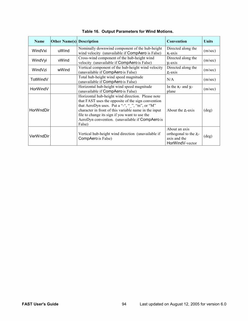
FAST User's Guide 94 Last updated on August 12, 2005 for version 6.0
Table 16. Output Parameters for Wind Motions.
Name Other Name(s) Description Convention Units
WindVxi uWind Nominally downwind component of the hub-height wind velocity (unavailable if CompAero is False)
Directed along the xi-axis (m/sec)
WindVyi vWind Cross-wind component of the hub-height wind velocity (unavailable if CompAero is False)
Directed along the yi-axis (m/sec)
WindVzi wWind Vertical component of the hub-height wind velocity (unavailable if CompAero is False)
Directed along the zi-axis (m/sec)
TotWindV Total hub-height wind speed magnitude (unavailable if CompAero is False) N/A (m/sec)
HorWindV Horizontal hub-height wind speed magnitude (unavailable if CompAero is False)
In the xi- and yi-plane (m/sec)
HorWndDir
Horizontal hub-height wind direction. Please note that FAST uses the opposite of the sign convention that AeroDyn uses. Put a “-“, “_”, “m”, or “M” character in front of this variable name in the input file to change its sign if you want to use the AeroDyn convention. (unavailable if CompAero is False)
About the zi-axis (deg)
VerWndDir Vertical hub-height wind direction (unavailable if CompAero is False)
About an axis orthogonal to the zi-axis and the HorWindV-vector
(deg)
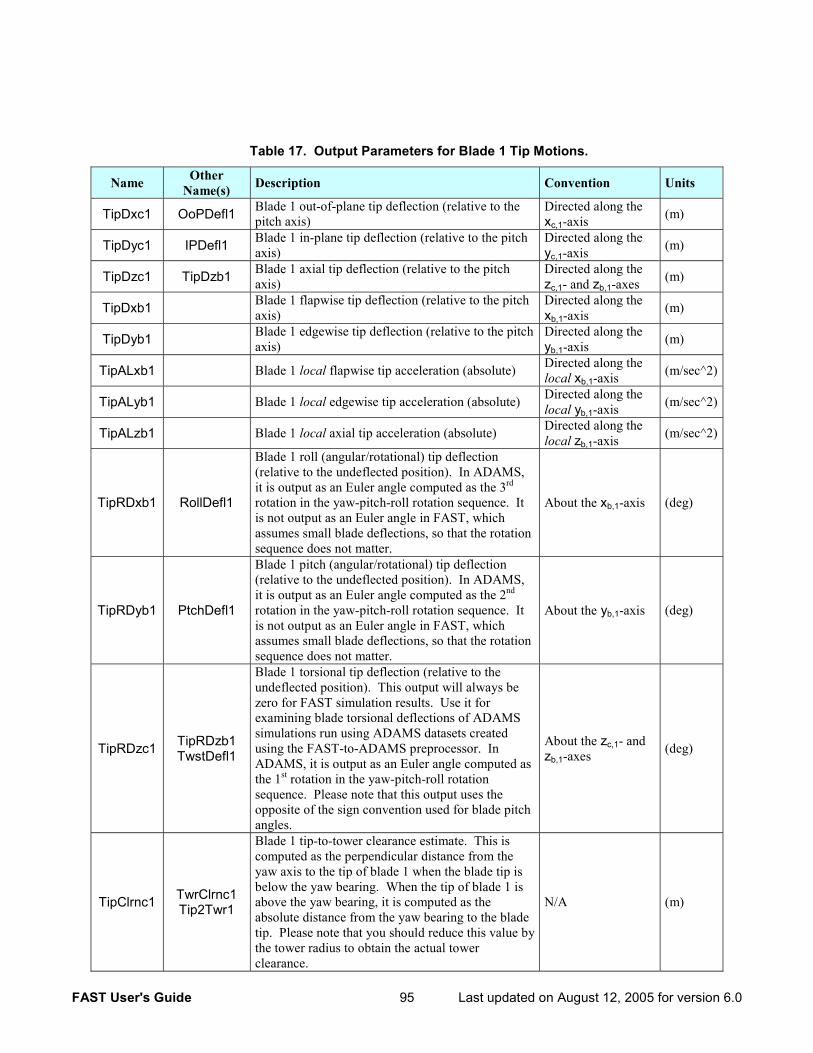
FAST User's Guide 95 Last updated on August 12, 2005 for version 6.0
Table 17. Output Parameters for Blade 1 Tip Motions.
Name Other Name(s) Description Convention Units
TipDxc1 OoPDefl1 Blade 1 out-of-plane tip deflection (relative to the pitch axis)
Directed along the xc,1-axis (m)
TipDyc1 IPDefl1 Blade 1 in-plane tip deflection (relative to the pitch axis)
Directed along the yc,1-axis (m)
TipDzc1 TipDzb1 Blade 1 axial tip deflection (relative to the pitch axis)
Directed along the zc,1- and zb,1-axes (m)
TipDxb1 Blade 1 flapwise tip deflection (relative to the pitch axis)
Directed along the xb,1-axis (m)
TipDyb1 Blade 1 edgewise tip deflection (relative to the pitch axis)
Directed along the yb,1-axis (m)
TipALxb1 Blade 1 local flapwise tip acceleration (absolute) Directed along the local xb,1-axis (m/sec^2)
TipALyb1 Blade 1 local edgewise tip acceleration (absolute) Directed along the local yb,1-axis (m/sec^2)
TipALzb1 Blade 1 local axial tip acceleration (absolute) Directed along the local zb,1-axis (m/sec^2)
TipRDxb1 RollDefl1
Blade 1 roll (angular/rotational) tip deflection (relative to the undeflected position). In ADAMS, it is output as an Euler angle computed as the 3rd rotation in the yaw-pitch-roll rotation sequence. It is not output as an Euler angle in FAST, which assumes small blade deflections, so that the rotation sequence does not matter.
About the xb,1-axis (deg)
TipRDyb1 PtchDefl1
Blade 1 pitch (angular/rotational) tip deflection (relative to the undeflected position). In ADAMS, it is output as an Euler angle computed as the 2nd rotation in the yaw-pitch-roll rotation sequence. It is not output as an Euler angle in FAST, which assumes small blade deflections, so that the rotation sequence does not matter.
About the yb,1-axis (deg)
TipRDzc1 TipRDzb1 TwstDefl1
Blade 1 torsional tip deflection (relative to the undeflected position). This output will always be zero for FAST simulation results. Use it for examining blade torsional deflections of ADAMS simulations run using ADAMS datasets created using the FAST-to-ADAMS preprocessor. In ADAMS, it is output as an Euler angle computed as the 1st rotation in the yaw-pitch-roll rotation sequence. Please note that this output uses the opposite of the sign convention used for blade pitch angles.
About the zc,1- and zb,1-axes (deg)
TipClrnc1 TwrClrnc1 Tip2Twr1
Blade 1 tip-to-tower clearance estimate. This is computed as the perpendicular distance from the yaw axis to the tip of blade 1 when the blade tip is below the yaw bearing. When the tip of blade 1 is above the yaw bearing, it is computed as the absolute distance from the yaw bearing to the blade tip. Please note that you should reduce this value by the tower radius to obtain the actual tower clearance.
N/A (m)
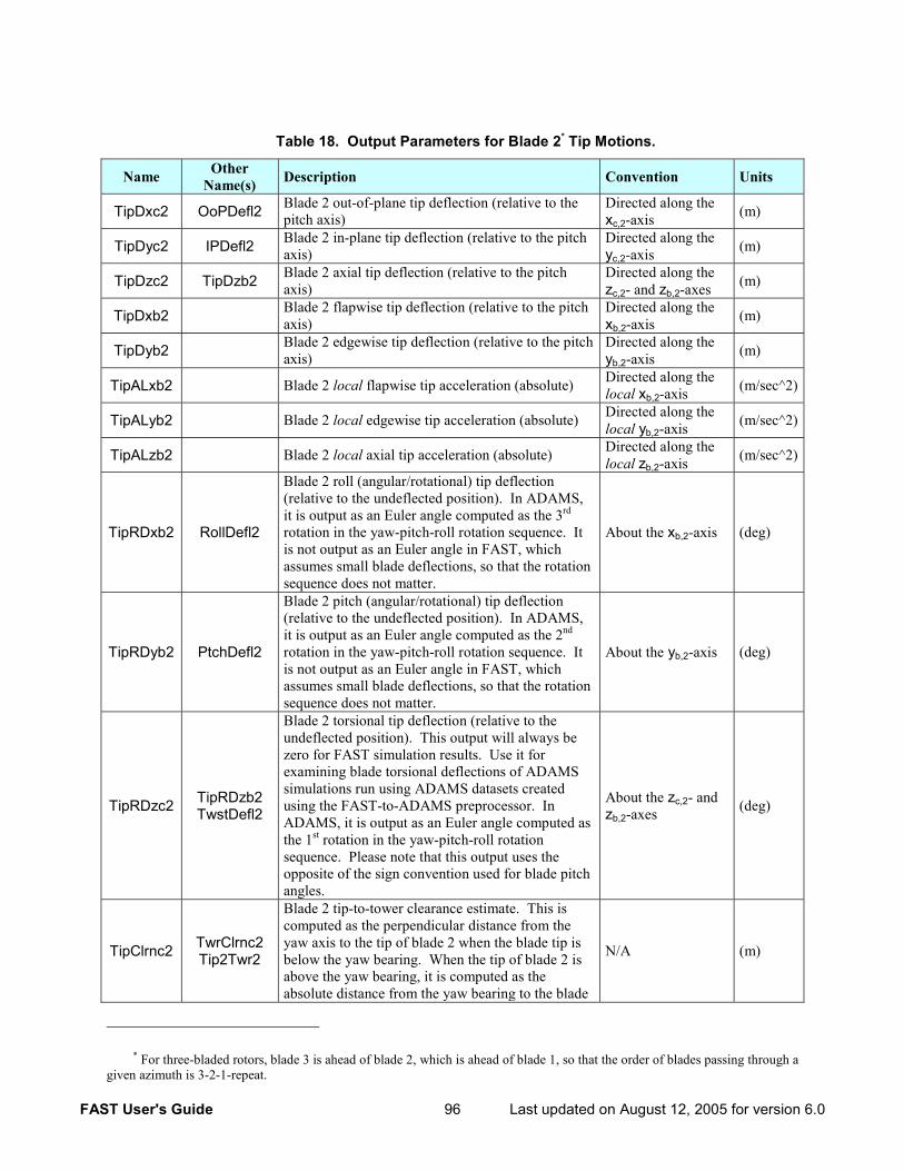
FAST User's Guide 96 Last updated on August 12, 2005 for version 6.0
Table 18. Output Parameters for Blade 2* Tip Motions.
Name Other Name(s) Description Convention Units
TipDxc2 OoPDefl2 Blade 2 out-of-plane tip deflection (relative to the pitch axis)
Directed along the xc,2-axis (m)
TipDyc2 IPDefl2 Blade 2 in-plane tip deflection (relative to the pitch axis)
Directed along the yc,2-axis (m)
TipDzc2 TipDzb2 Blade 2 axial tip deflection (relative to the pitch axis)
Directed along the zc,2- and zb,2-axes (m)
TipDxb2 Blade 2 flapwise tip deflection (relative to the pitch axis)
Directed along the xb,2-axis (m)
TipDyb2 Blade 2 edgewise tip deflection (relative to the pitch axis)
Directed along the yb,2-axis (m)
TipALxb2 Blade 2 local flapwise tip acceleration (absolute) Directed along the local xb,2-axis (m/sec^2)
TipALyb2 Blade 2 local edgewise tip acceleration (absolute) Directed along the local yb,2-axis (m/sec^2)
TipALzb2 Blade 2 local axial tip acceleration (absolute) Directed along the local zb,2-axis (m/sec^2)
TipRDxb2 RollDefl2
Blade 2 roll (angular/rotational) tip deflection (relative to the undeflected position). In ADAMS, it is output as an Euler angle computed as the 3rd rotation in the yaw-pitch-roll rotation sequence. It is not output as an Euler angle in FAST, which assumes small blade deflections, so that the rotation sequence does not matter.
About the xb,2-axis (deg)
TipRDyb2 PtchDefl2
Blade 2 pitch (angular/rotational) tip deflection (relative to the undeflected position). In ADAMS, it is output as an Euler angle computed as the 2nd rotation in the yaw-pitch-roll rotation sequence. It is not output as an Euler angle in FAST, which assumes small blade deflections, so that the rotation sequence does not matter.
About the yb,2-axis (deg)
TipRDzc2 TipRDzb2 TwstDefl2
Blade 2 torsional tip deflection (relative to the undeflected position). This output will always be zero for FAST simulation results. Use it for examining blade torsional deflections of ADAMS simulations run using ADAMS datasets created using the FAST-to-ADAMS preprocessor. In ADAMS, it is output as an Euler angle computed as the 1st rotation in the yaw-pitch-roll rotation sequence. Please note that this output uses the opposite of the sign convention used for blade pitch angles.
About the zc,2- and zb,2-axes (deg)
TipClrnc2 TwrClrnc2 Tip2Twr2
Blade 2 tip-to-tower clearance estimate. This is computed as the perpendicular distance from the yaw axis to the tip of blade 2 when the blade tip is below the yaw bearing. When the tip of blade 2 is above the yaw bearing, it is computed as the absolute distance from the yaw bearing to the blade
N/A (m)
* For three-bladed rotors, blade 3 is ahead of blade 2, which is ahead of blade 1, so that the order of blades passing through a given azimuth is 3-2-1-repeat.

FAST User's Guide 97 Last updated on August 12, 2005 for version 6.0
Name Other Name(s) Description Convention Units
tip. Please note that you should reduce this value by the tower radius to obtain the actual tower clearance.
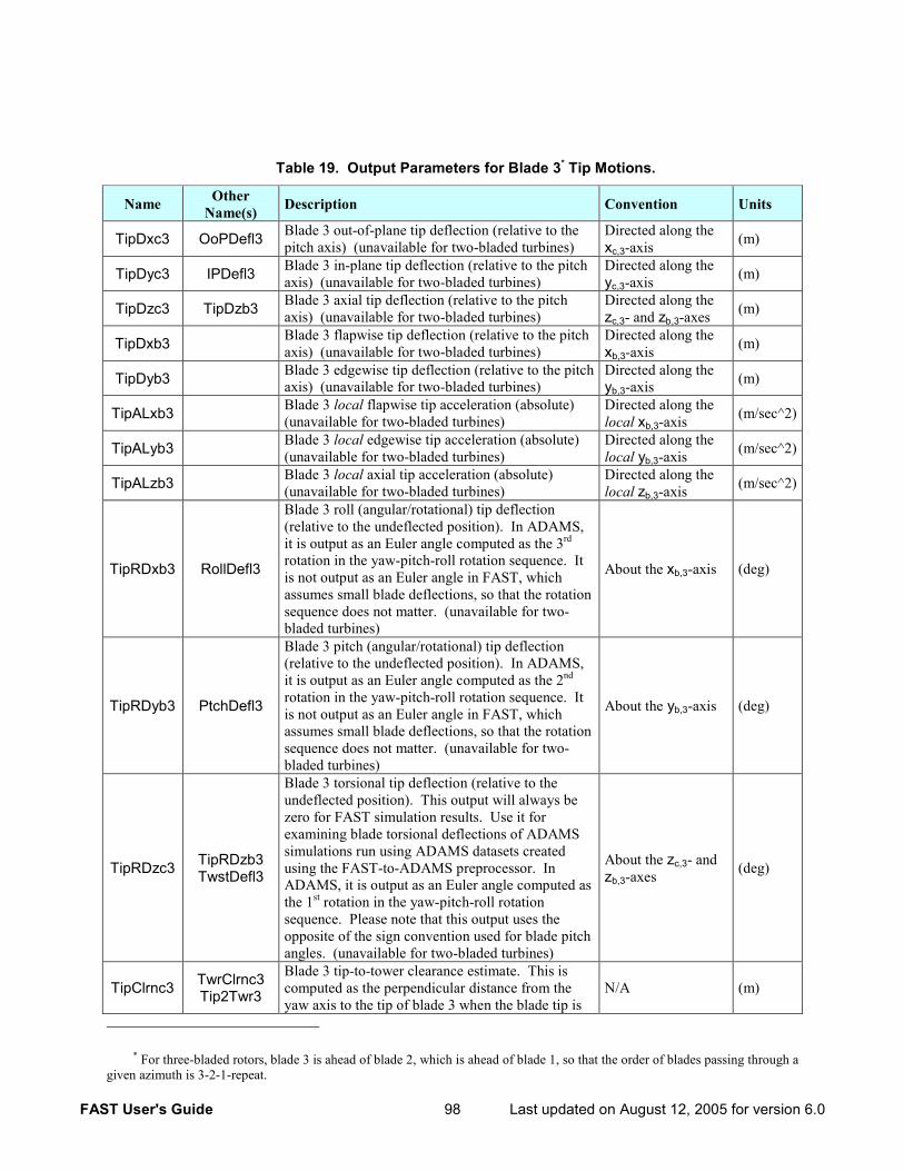
FAST User's Guide 98 Last updated on August 12, 2005 for version 6.0
Table 19. Output Parameters for Blade 3* Tip Motions.
Name Other Name(s) Description Convention Units
TipDxc3 OoPDefl3 Blade 3 out-of-plane tip deflection (relative to the pitch axis) (unavailable for two-bladed turbines)
Directed along the xc,3-axis (m)
TipDyc3 IPDefl3 Blade 3 in-plane tip deflection (relative to the pitch axis) (unavailable for two-bladed turbines)
Directed along the yc,3-axis (m)
TipDzc3 TipDzb3 Blade 3 axial tip deflection (relative to the pitch axis) (unavailable for two-bladed turbines)
Directed along the zc,3- and zb,3-axes (m)
TipDxb3 Blade 3 flapwise tip deflection (relative to the pitch axis) (unavailable for two-bladed turbines)
Directed along the xb,3-axis (m)
TipDyb3 Blade 3 edgewise tip deflection (relative to the pitch axis) (unavailable for two-bladed turbines)
Directed along the yb,3-axis (m)
TipALxb3 Blade 3 local flapwise tip acceleration (absolute) (unavailable for two-bladed turbines)
Directed along the local xb,3-axis (m/sec^2)
TipALyb3 Blade 3 local edgewise tip acceleration (absolute) (unavailable for two-bladed turbines)
Directed along the local yb,3-axis (m/sec^2)
TipALzb3 Blade 3 local axial tip acceleration (absolute) (unavailable for two-bladed turbines)
Directed along the local zb,3-axis (m/sec^2)
TipRDxb3 RollDefl3
Blade 3 roll (angular/rotational) tip deflection (relative to the undeflected position). In ADAMS, it is output as an Euler angle computed as the 3rd rotation in the yaw-pitch-roll rotation sequence. It is not output as an Euler angle in FAST, which assumes small blade deflections, so that the rotation sequence does not matter. (unavailable for two-bladed turbines)
About the xb,3-axis (deg)
TipRDyb3 PtchDefl3
Blade 3 pitch (angular/rotational) tip deflection (relative to the undeflected position). In ADAMS, it is output as an Euler angle computed as the 2nd rotation in the yaw-pitch-roll rotation sequence. It is not output as an Euler angle in FAST, which assumes small blade deflections, so that the rotation sequence does not matter. (unavailable for two-bladed turbines)
About the yb,3-axis (deg)
TipRDzc3 TipRDzb3 TwstDefl3
Blade 3 torsional tip deflection (relative to the undeflected position). This output will always be zero for FAST simulation results. Use it for examining blade torsional deflections of ADAMS simulations run using ADAMS datasets created using the FAST-to-ADAMS preprocessor. In ADAMS, it is output as an Euler angle computed as the 1st rotation in the yaw-pitch-roll rotation sequence. Please note that this output uses the opposite of the sign convention used for blade pitch angles. (unavailable for two-bladed turbines)
About the zc,3- and zb,3-axes (deg)
TipClrnc3 TwrClrnc3 Tip2Twr3
Blade 3 tip-to-tower clearance estimate. This is computed as the perpendicular distance from the yaw axis to the tip of blade 3 when the blade tip is
N/A (m)
* For three-bladed rotors, blade 3 is ahead of blade 2, which is ahead of blade 1, so that the order of blades passing through a given azimuth is 3-2-1-repeat.

FAST User's Guide 99 Last updated on August 12, 2005 for version 6.0
Name Other Name(s) Description Convention Units
below the yaw bearing. When the tip of blade 3 is above the yaw bearing, it is computed as the absolute distance from the yaw bearing to the blade tip. Please note that you should reduce this value by the tower radius to obtain the actual tower clearance. (unavailable for two-bladed turbines)
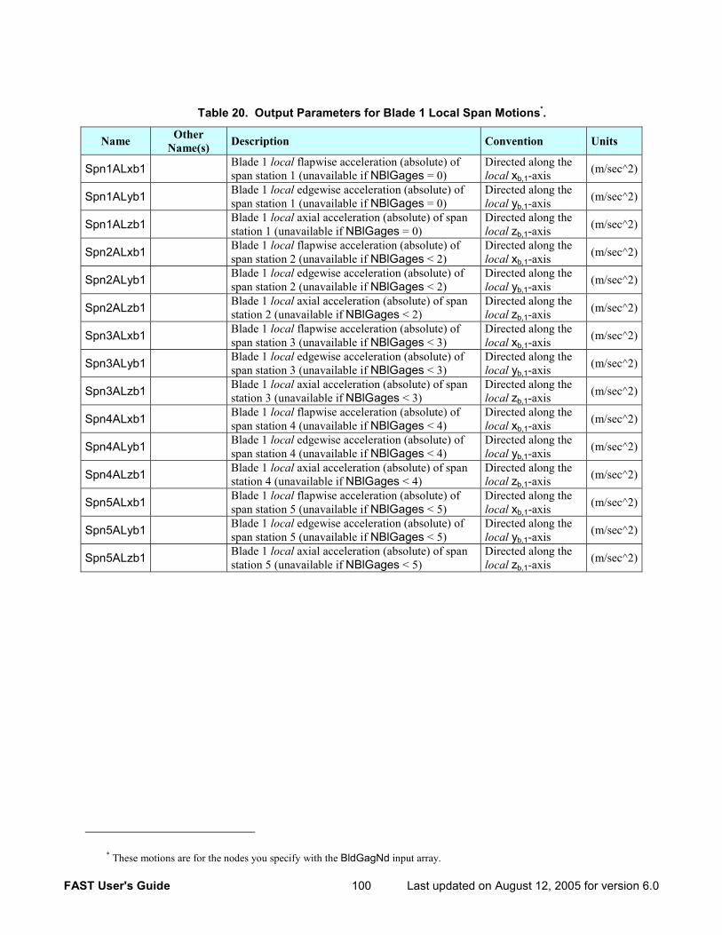
FAST User's Guide 100 Last updated on August 12, 2005 for version 6.0
Table 20. Output Parameters for Blade 1 Local Span Motions*.
Name Other Name(s) Description Convention Units
Spn1ALxb1 Blade 1 local flapwise acceleration (absolute) of span station 1 (unavailable if NBlGages = 0)
Directed along the local xb,1-axis (m/sec^2)
Spn1ALyb1 Blade 1 local edgewise acceleration (absolute) of span station 1 (unavailable if NBlGages = 0)
Directed along the local yb,1-axis (m/sec^2)
Spn1ALzb1 Blade 1 local axial acceleration (absolute) of span station 1 (unavailable if NBlGages = 0)
Directed along the local zb,1-axis (m/sec^2)
Spn2ALxb1 Blade 1 local flapwise acceleration (absolute) of span station 2 (unavailable if NBlGages < 2)
Directed along the local xb,1-axis (m/sec^2)
Spn2ALyb1 Blade 1 local edgewise acceleration (absolute) of span station 2 (unavailable if NBlGages < 2)
Directed along the local yb,1-axis (m/sec^2)
Spn2ALzb1 Blade 1 local axial acceleration (absolute) of span station 2 (unavailable if NBlGages < 2)
Directed along the local zb,1-axis (m/sec^2)
Spn3ALxb1 Blade 1 local flapwise acceleration (absolute) of span station 3 (unavailable if NBlGages < 3)
Directed along the local xb,1-axis (m/sec^2)
Spn3ALyb1 Blade 1 local edgewise acceleration (absolute) of span station 3 (unavailable if NBlGages < 3)
Directed along the local yb,1-axis (m/sec^2)
Spn3ALzb1 Blade 1 local axial acceleration (absolute) of span station 3 (unavailable if NBlGages < 3)
Directed along the local zb,1-axis (m/sec^2)
Spn4ALxb1 Blade 1 local flapwise acceleration (absolute) of span station 4 (unavailable if NBlGages < 4)
Directed along the local xb,1-axis (m/sec^2)
Spn4ALyb1 Blade 1 local edgewise acceleration (absolute) of span station 4 (unavailable if NBlGages < 4)
Directed along the local yb,1-axis (m/sec^2)
Spn4ALzb1 Blade 1 local axial acceleration (absolute) of span station 4 (unavailable if NBlGages < 4)
Directed along the local zb,1-axis (m/sec^2)
Spn5ALxb1 Blade 1 local flapwise acceleration (absolute) of span station 5 (unavailable if NBlGages < 5)
Directed along the local xb,1-axis (m/sec^2)
Spn5ALyb1 Blade 1 local edgewise acceleration (absolute) of span station 5 (unavailable if NBlGages < 5)
Directed along the local yb,1-axis (m/sec^2)
Spn5ALzb1 Blade 1 local axial acceleration (absolute) of span station 5 (unavailable if NBlGages < 5)
Directed along the local zb,1-axis (m/sec^2)
* These motions are for the nodes you specify with the BldGagNd input array.
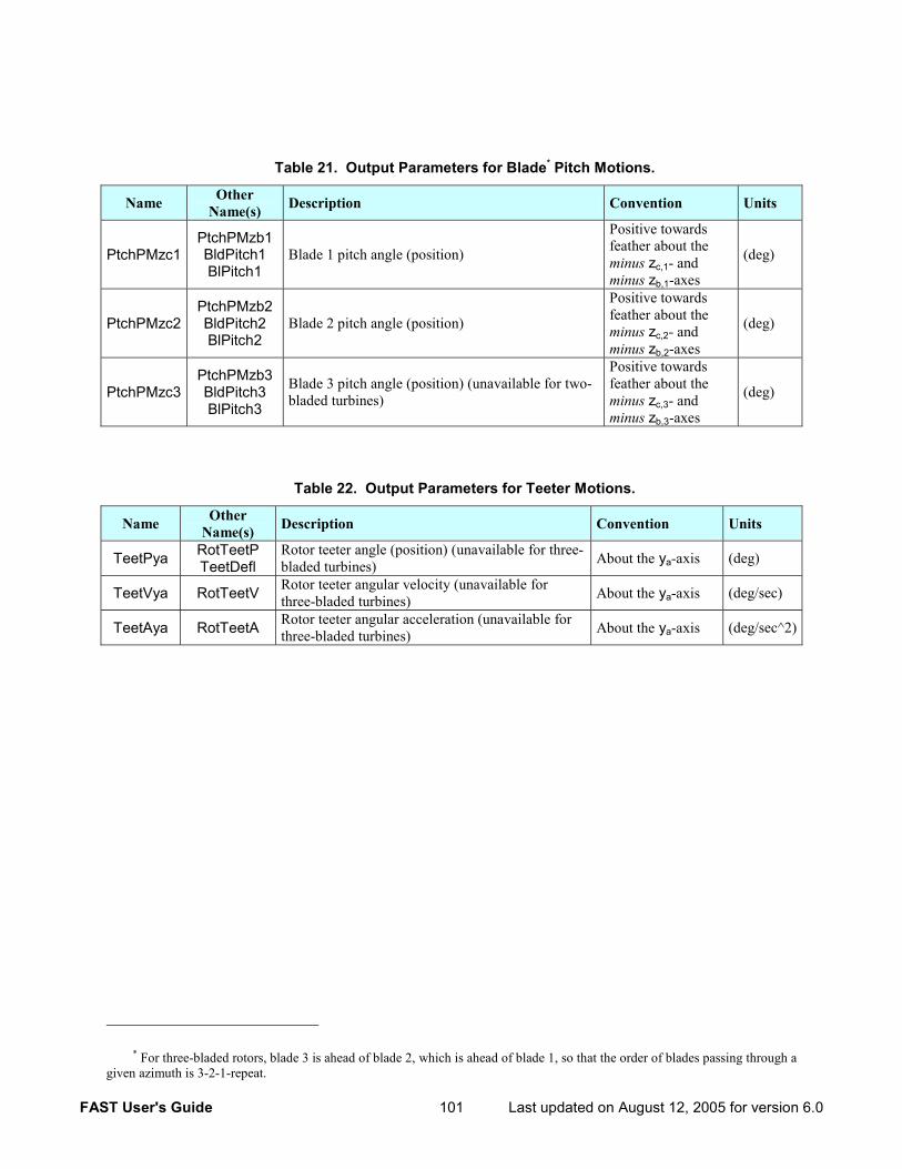
FAST User's Guide 101 Last updated on August 12, 2005 for version 6.0
Table 21. Output Parameters for Blade* Pitch Motions.
Name Other Name(s) Description Convention Units
PtchPMzc1 PtchPMzb1 BldPitch1 BlPitch1
Blade 1 pitch angle (position)
Positive towards feather about the minus zc,1- and minus zb,1-axes
(deg)
PtchPMzc2 PtchPMzb2 BldPitch2 BlPitch2
Blade 2 pitch angle (position)
Positive towards feather about the minus zc,2- and minus zb,2-axes
(deg)
PtchPMzc3 PtchPMzb3 BldPitch3 BlPitch3
Blade 3 pitch angle (position) (unavailable for two-bladed turbines)
Positive towards feather about the minus zc,3- and minus zb,3-axes
(deg)
Table 22. Output Parameters for Teeter Motions.
Name Other Name(s) Description Convention Units
TeetPya RotTeetP TeetDefl
Rotor teeter angle (position) (unavailable for three-bladed turbines) About the ya-axis (deg)
TeetVya RotTeetV Rotor teeter angular velocity (unavailable for three-bladed turbines) About the ya-axis (deg/sec)
TeetAya RotTeetA Rotor teeter angular acceleration (unavailable for three-bladed turbines) About the ya-axis (deg/sec^2)
* For three-bladed rotors, blade 3 is ahead of blade 2, which is ahead of blade 1, so that the order of blades passing through a given azimuth is 3-2-1-repeat.
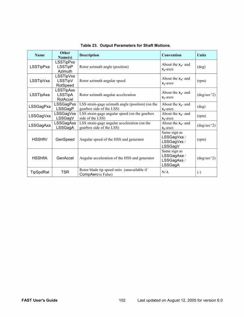
FAST User's Guide 102 Last updated on August 12, 2005 for version 6.0
Table 23. Output Parameters for Shaft Motions.
Name Other Name(s) Description Convention Units
LSSTipPxa LSSTipPxs LSSTipP Azimuth
Rotor azimuth angle (position) About the xa- and xs-axes (deg)
LSSTipVxa LSSTipVxs LSSTipV RotSpeed
Rotor azimuth angular speed About the xa- and xs-axes (rpm)
LSSTipAxa LSSTipAxs LSSTipA RotAccel
Rotor azimuth angular acceleration About the xa- and xs-axes (deg/sec^2)
LSSGagPxa LSSGagPxs LSSGagP
LSS strain-gage azimuth angle (position) (on the gearbox side of the LSS)
About the xa- and xs-axes (deg)
LSSGagVxa LSSGagVxs LSSGagV
LSS strain-gage angular speed (on the gearbox side of the LSS)
About the xa- and xs-axes (rpm)
LSSGagAxa LSSGagAxs LSSGagA
LSS strain-gage angular acceleration (on the gearbox side of the LSS)
About the xa- and xs-axes (deg/sec^2)
HSShftV GenSpeed Angular speed of the HSS and generator
Same sign as LSSGagVxa / LSSGagVxs / LSSGagV
(rpm)
HSShftA GenAccel Angular acceleration of the HSS and generator
Same sign as LSSGagAxa / LSSGagAxs / LSSGagA
(deg/sec^2)
TipSpdRat TSR Rotor blade tip speed ratio (unavailable if CompAero is False) N/A (-)
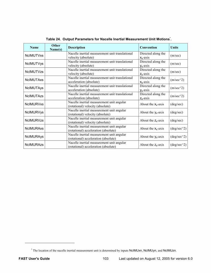
FAST User's Guide 103 Last updated on August 12, 2005 for version 6.0
Table 24. Output Parameters for Nacelle Inertial Measurement Unit Motions*.
Name Other Name(s) Description Convention Units
NcIMUTVxs Nacelle inertial measurement unit translational velocity (absolute)
Directed along the xs-axis (m/sec)
NcIMUTVys Nacelle inertial measurement unit translational velocity (absolute)
Directed along the ys-axis (m/sec)
NcIMUTVzs Nacelle inertial measurement unit translational velocity (absolute)
Directed along the zs-axis (m/sec)
NcIMUTAxs Nacelle inertial measurement unit translational acceleration (absolute)
Directed along the xs-axis (m/sec^2)
NcIMUTAys Nacelle inertial measurement unit translational acceleration (absolute)
Directed along the ys-axis (m/sec^2)
NcIMUTAzs Nacelle inertial measurement unit translational acceleration (absolute)
Directed along the zs-axis (m/sec^2)
NcIMURVxs Nacelle inertial measurement unit angular (rotational) velocity (absolute) About the xs-axis (deg/sec)
NcIMURVys Nacelle inertial measurement unit angular (rotational) velocity (absolute) About the ys-axis (deg/sec)
NcIMURVzs Nacelle inertial measurement unit angular (rotational) velocity (absolute) About the zs-axis (deg/sec)
NcIMURAxs Nacelle inertial measurement unit angular (rotational) acceleration (absolute) About the xs-axis (deg/sec^2)
NcIMURAys Nacelle inertial measurement unit angular (rotational) acceleration (absolute) About the ys-axis (deg/sec^2)
NcIMURAzs Nacelle inertial measurement unit angular (rotational) acceleration (absolute) About the zs-axis (deg/sec^2)
* The location of the nacelle inertial measurement unit is determined by inputs NcIMUxn, NcIMUyn, and NcIMUzn.
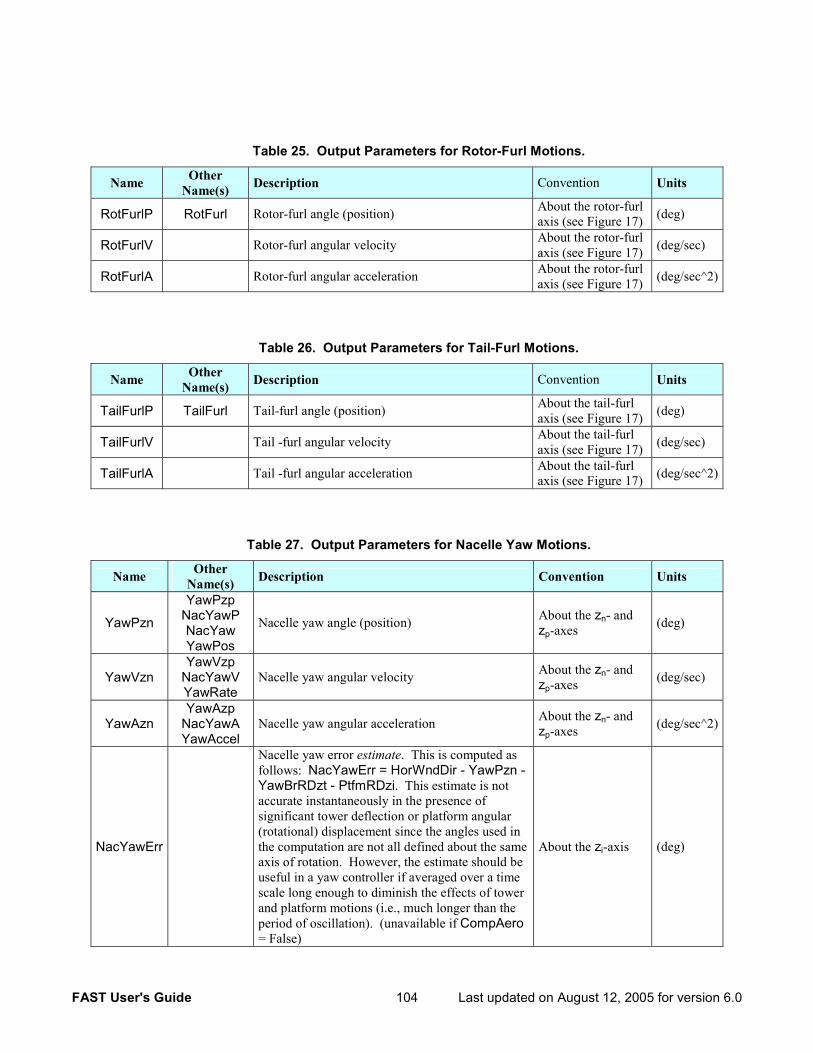
FAST User's Guide 104 Last updated on August 12, 2005 for version 6.0
Table 25. Output Parameters for Rotor-Furl Motions.
Name Other Name(s) Description Convention Units
RotFurlP RotFurl Rotor-furl angle (position) About the rotor-furl axis (see Figure 17) (deg)
RotFurlV Rotor-furl angular velocity About the rotor-furl axis (see Figure 17) (deg/sec)
RotFurlA Rotor-furl angular acceleration About the rotor-furl axis (see Figure 17) (deg/sec^2)
Table 26. Output Parameters for Tail-Furl Motions.
Name Other Name(s) Description Convention Units
TailFurlP TailFurl Tail-furl angle (position) About the tail-furl axis (see Figure 17) (deg)
TailFurlV Tail -furl angular velocity About the tail-furl axis (see Figure 17) (deg/sec)
TailFurlA Tail -furl angular acceleration About the tail-furl axis (see Figure 17) (deg/sec^2)
Table 27. Output Parameters for Nacelle Yaw Motions.
Name Other Name(s) Description Convention Units
YawPzn
YawPzp NacYawP NacYaw YawPos
Nacelle yaw angle (position) About the zn- and zp-axes (deg)
YawVzn YawVzp
NacYawV YawRate
Nacelle yaw angular velocity About the zn- and zp-axes (deg/sec)
YawAzn YawAzp
NacYawA YawAccel
Nacelle yaw angular acceleration About the zn- and zp-axes (deg/sec^2)
NacYawErr
Nacelle yaw error estimate. This is computed as follows: NacYawErr = HorWndDir - YawPzn - YawBrRDzt - PtfmRDzi. This estimate is not accurate instantaneously in the presence of significant tower deflection or platform angular (rotational) displacement since the angles used in the computation are not all defined about the same axis of rotation. However, the estimate should be useful in a yaw controller if averaged over a time scale long enough to diminish the effects of tower and platform motions (i.e., much longer than the period of oscillation). (unavailable if CompAero = False)
About the zi-axis (deg)
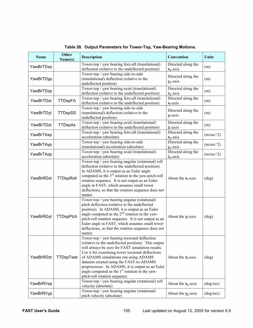
FAST User's Guide 105 Last updated on August 12, 2005 for version 6.0
Table 28. Output Parameters for Tower-Top, Yaw-Bearing Motions.
Name Other Name(s) Description Convention Units
YawBrTDxp Tower-top / yaw bearing fore-aft (translational) deflection (relative to the undeflected position)
Directed along the xp-axis (m)
YawBrTDyp Tower-top / yaw bearing side-to-side (translational) deflection (relative to the undeflected position)
Directed along the yp-axis (m)
YawBrTDzp Tower-top / yaw bearing axial (translational) deflection (relative to the undeflected position)
Directed along the zp-axis (m)
YawBrTDxt TTDspFA Tower-top / yaw bearing fore-aft (translational) deflection (relative to the undeflected position)
Directed along the xt-axis (m)
YawBrTDyt TTDspSS Tower-top / yaw bearing side-to-side (translational) deflection (relative to the undeflected position)
Directed along the yt-axis (m)
YawBrTDzt TTDspAx Tower-top / yaw bearing axial (translational) deflection (relative to the undeflected position)
Directed along the zt-axis (m)
YawBrTAxp Tower-top / yaw bearing fore-aft (translational) acceleration (absolute)
Directed along the xp-axis (m/sec^2)
YawBrTAyp Tower-top / yaw bearing side-to-side (translational) acceleration (absolute)
Directed along the yp-axis (m/sec^2)
YawBrTAzp Tower-top / yaw bearing axial (translational) acceleration (absolute)
Directed along the zp-axis (m/sec^2)
YawBrRDxt TTDspRoll
Tower-top / yaw bearing angular (rotational) roll deflection (relative to the undeflected position). In ADAMS, it is output as an Euler angle computed as the 3rd rotation in the yaw-pitch-roll rotation sequence. It is not output as an Euler angle in FAST, which assumes small tower deflections, so that the rotation sequence does not matter.
About the xt-axis (deg)
YawBrRDyt TTDspPtch
Tower-top / yaw bearing angular (rotational) pitch deflection (relative to the undeflected position). In ADAMS, it is output as an Euler angle computed as the 2nd rotation in the yaw-pitch-roll rotation sequence. It is not output as an Euler angle in FAST, which assumes small tower deflections, so that the rotation sequence does not matter.
About the yt-axis (deg)
YawBrRDzt TTDspTwst
Tower-top / yaw bearing torsional deflection (relative to the undeflected position). This output will always be zero for FAST simulation results. Use it for examining tower torsional deflections of ADAMS simulations run using ADAMS datasets created using the FAST-to-ADAMS preprocessor. In ADAMS, it is output as an Euler angle computed as the 1st rotation in the yaw-pitch-roll rotation sequence.
About the zt-axis (deg)
YawBrRVxp Tower-top / yaw bearing angular (rotational) roll velocity (absolute) About the xp-axis (deg/sec)
YawBrRVyp Tower-top / yaw bearing angular (rotational) pitch velocity (absolute) About the yp-axis (deg/sec)
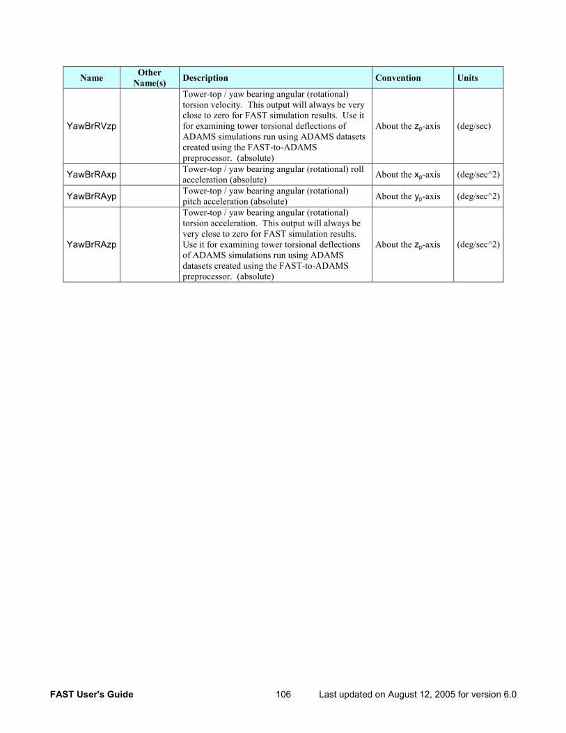
FAST User's Guide 106 Last updated on August 12, 2005 for version 6.0
Name Other Name(s) Description Convention Units
YawBrRVzp
Tower-top / yaw bearing angular (rotational) torsion velocity. This output will always be very close to zero for FAST simulation results. Use it for examining tower torsional deflections of ADAMS simulations run using ADAMS datasets created using the FAST-to-ADAMS preprocessor. (absolute)
About the zp-axis (deg/sec)
YawBrRAxp Tower-top / yaw bearing angular (rotational) roll acceleration (absolute) About the xp-axis (deg/sec^2)
YawBrRAyp Tower-top / yaw bearing angular (rotational) pitch acceleration (absolute) About the yp-axis (deg/sec^2)
YawBrRAzp
Tower-top / yaw bearing angular (rotational) torsion acceleration. This output will always be very close to zero for FAST simulation results. Use it for examining tower torsional deflections of ADAMS simulations run using ADAMS datasets created using the FAST-to-ADAMS preprocessor. (absolute)
About the zp-axis (deg/sec^2)
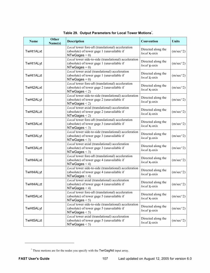
FAST User's Guide 107 Last updated on August 12, 2005 for version 6.0
Table 29. Output Parameters for Local Tower Motions*.
Name Other Name(s) Description Convention Units
TwHt1ALxt Local tower fore-aft (translational) acceleration (absolute) of tower gage 1 (unavailable if NTwGages = 0)
Directed along the local xt-axis (m/sec^2)
TwHt1ALyt Local tower side-to-side (translational) acceleration (absolute) of tower gage 1 (unavailable if NTwGages = 0)
Directed along the local yt-axis (m/sec^2)
TwHt1ALzt Local tower axial (translational) acceleration (absolute) of tower gage 1 (unavailable if NTwGages = 0)
Directed along the local zt-axis (m/sec^2)
TwHt2ALxt Local tower fore-aft (translational) acceleration (absolute) of tower gage 2 (unavailable if NTwGages < 2)
Directed along the local xt-axis (m/sec^2)
TwHt2ALyt Local tower side-to-side (translational) acceleration (absolute) of tower gage 2 (unavailable if NTwGages < 2)
Directed along the local yt-axis (m/sec^2)
TwHt2ALzt Local tower axial (translational) acceleration (absolute) of tower gage 2 (unavailable if NTwGages < 2)
Directed along the local zt-axis (m/sec^2)
TwHt3ALxt Local tower fore-aft (translational) acceleration (absolute) of tower gage 3 (unavailable if NTwGages < 3)
Directed along the local xt-axis (m/sec^2)
TwHt3ALyt Local tower side-to-side (translational) acceleration (absolute) of tower gage 3 (unavailable if NTwGages < 3)
Directed along the local yt-axis (m/sec^2)
TwHt3ALzt Local tower axial (translational) acceleration (absolute) of tower gage 3 (unavailable if NTwGages < 3)
Directed along the local zt-axis (m/sec^2)
TwHt4ALxt Local tower fore-aft (translational) acceleration (absolute) of tower gage 4 (unavailable if NTwGages < 4)
Directed along the local xt-axis (m/sec^2)
TwHt4ALyt Local tower side-to-side (translational) acceleration (absolute) of tower gage 4 (unavailable if NTwGages < 4)
Directed along the local yt-axis (m/sec^2)
TwHt4ALzt Local tower axial (translational) acceleration (absolute) of tower gage 4 (unavailable if NTwGages < 4)
Directed along the local zt-axis (m/sec^2)
TwHt5ALxt Local tower fore-aft (translational) acceleration (absolute) of tower gage 5 (unavailable if NTwGages < 5)
Directed along the local xt-axis (m/sec^2)
TwHt5ALyt Local tower side-to-side (translational) acceleration (absolute) of tower gage 5 (unavailable if NTwGages < 5)
Directed along the local yt-axis (m/sec^2)
TwHt5ALzt Local tower axial (translational) acceleration (absolute) of tower gage 5 (unavailable if NTwGages < 5)
Directed along the local zt-axis (m/sec^2)
* These motions are for the nodes you specify with the TwrGagNd input array.
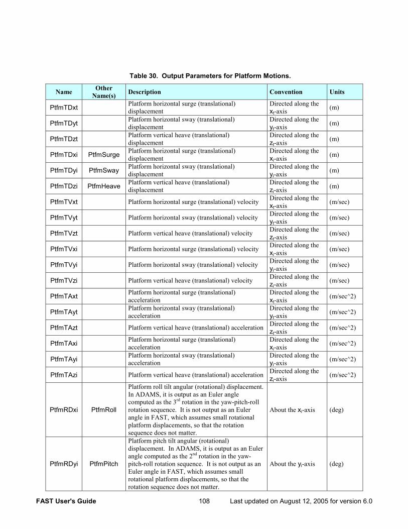
FAST User's Guide 108 Last updated on August 12, 2005 for version 6.0
Table 30. Output Parameters for Platform Motions.
Name Other Name(s) Description Convention Units
PtfmTDxt Platform horizontal surge (translational) displacement
Directed along the xt-axis (m)
PtfmTDyt Platform horizontal sway (translational) displacement
Directed along the yt-axis (m)
PtfmTDzt Platform vertical heave (translational) displacement
Directed along the zt-axis (m)
PtfmTDxi PtfmSurge Platform horizontal surge (translational) displacement
Directed along the xi-axis (m)
PtfmTDyi PtfmSway Platform horizontal sway (translational) displacement
Directed along the yi-axis (m)
PtfmTDzi PtfmHeave Platform vertical heave (translational) displacement
Directed along the zi-axis (m)
PtfmTVxt Platform horizontal surge (translational) velocity Directed along the xt-axis (m/sec)
PtfmTVyt Platform horizontal sway (translational) velocity Directed along the yt-axis (m/sec)
PtfmTVzt Platform vertical heave (translational) velocity Directed along the zt-axis (m/sec)
PtfmTVxi Platform horizontal surge (translational) velocity Directed along the xi-axis (m/sec)
PtfmTVyi Platform horizontal sway (translational) velocity Directed along the yi-axis (m/sec)
PtfmTVzi Platform vertical heave (translational) velocity Directed along the zi-axis (m/sec)
PtfmTAxt Platform horizontal surge (translational) acceleration
Directed along the xt-axis (m/sec^2)
PtfmTAyt Platform horizontal sway (translational) acceleration
Directed along the yt-axis (m/sec^2)
PtfmTAzt Platform vertical heave (translational) acceleration Directed along the zt-axis (m/sec^2)
PtfmTAxi Platform horizontal surge (translational) acceleration
Directed along the xi-axis (m/sec^2)
PtfmTAyi Platform horizontal sway (translational) acceleration
Directed along the yi-axis (m/sec^2)
PtfmTAzi Platform vertical heave (translational) acceleration Directed along the zi-axis (m/sec^2)
PtfmRDxi PtfmRoll
Platform roll tilt angular (rotational) displacement. In ADAMS, it is output as an Euler angle computed as the 3rd rotation in the yaw-pitch-roll rotation sequence. It is not output as an Euler angle in FAST, which assumes small rotational platform displacements, so that the rotation sequence does not matter.
About the xi-axis (deg)
PtfmRDyi PtfmPitch
Platform pitch tilt angular (rotational) displacement. In ADAMS, it is output as an Euler angle computed as the 2nd rotation in the yaw-pitch-roll rotation sequence. It is not output as an Euler angle in FAST, which assumes small rotational platform displacements, so that the rotation sequence does not matter.
About the yi-axis (deg)
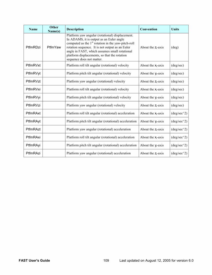
FAST User's Guide 109 Last updated on August 12, 2005 for version 6.0
Name Other Name(s) Description Convention Units
PtfmRDzi PtfmYaw
Platform yaw angular (rotational) displacement. In ADAMS, it is output as an Euler angle computed as the 1st rotation in the yaw-pitch-roll rotation sequence. It is not output as an Euler angle in FAST, which assumes small rotational platform displacements, so that the rotation sequence does not matter.
About the zi-axis (deg)
PtfmRVxt Platform roll tilt angular (rotational) velocity About the xt-axis (deg/sec)
PtfmRVyt Platform pitch tilt angular (rotational) velocity About the yt-axis (deg/sec)
PtfmRVzt Platform yaw angular (rotational) velocity About the zt-axis (deg/sec)
PtfmRVxi Platform roll tilt angular (rotational) velocity About the xi-axis (deg/sec)
PtfmRVyi Platform pitch tilt angular (rotational) velocity About the yi-axis (deg/sec)
PtfmRVzi Platform yaw angular (rotational) velocity About the zi-axis (deg/sec)
PtfmRAxt Platform roll tilt angular (rotational) acceleration About the xt-axis (deg/sec^2)
PtfmRAyt Platform pitch tilt angular (rotational) acceleration About the yt-axis (deg/sec^2)
PtfmRAzt Platform yaw angular (rotational) acceleration About the zt-axis (deg/sec^2)
PtfmRAxi Platform roll tilt angular (rotational) acceleration About the xi-axis (deg/sec^2)
PtfmRAyi Platform pitch tilt angular (rotational) acceleration About the yi-axis (deg/sec^2)
PtfmRAzi Platform yaw angular (rotational) acceleration About the zi-axis (deg/sec^2)
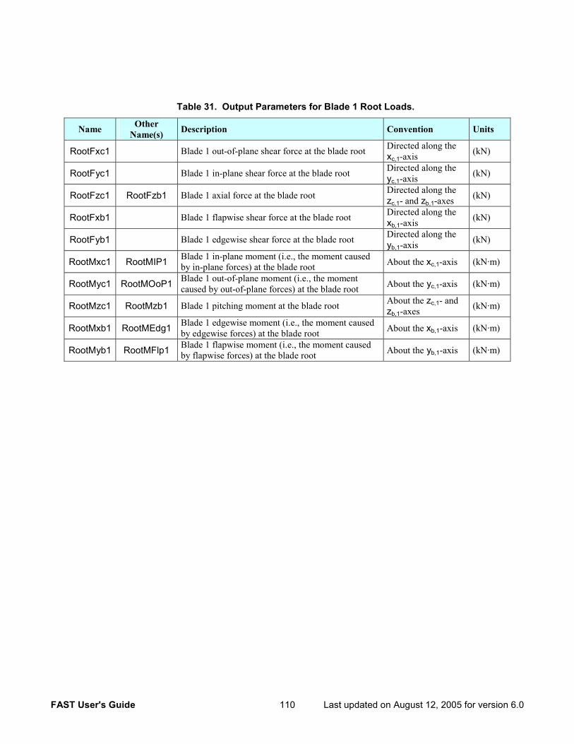
FAST User's Guide 110 Last updated on August 12, 2005 for version 6.0
Table 31. Output Parameters for Blade 1 Root Loads.
Name Other Name(s) Description Convention Units
RootFxc1 Blade 1 out-of-plane shear force at the blade root Directed along the xc,1-axis (kN)
RootFyc1 Blade 1 in-plane shear force at the blade root Directed along the yc,1-axis (kN)
RootFzc1 RootFzb1 Blade 1 axial force at the blade root Directed along the zc,1- and zb,1-axes (kN)
RootFxb1 Blade 1 flapwise shear force at the blade root Directed along the xb,1-axis (kN)
RootFyb1 Blade 1 edgewise shear force at the blade root Directed along the yb,1-axis (kN)
RootMxc1 RootMIP1 Blade 1 in-plane moment (i.e., the moment caused by in-plane forces) at the blade root About the xc,1-axis (kN·m)
RootMyc1 RootMOoP1 Blade 1 out-of-plane moment (i.e., the moment caused by out-of-plane forces) at the blade root About the yc,1-axis (kN·m)
RootMzc1 RootMzb1 Blade 1 pitching moment at the blade root About the zc,1- and zb,1-axes (kN·m)
RootMxb1 RootMEdg1 Blade 1 edgewise moment (i.e., the moment caused by edgewise forces) at the blade root About the xb,1-axis (kN·m)
RootMyb1 RootMFlp1 Blade 1 flapwise moment (i.e., the moment caused by flapwise forces) at the blade root About the yb,1-axis (kN·m)
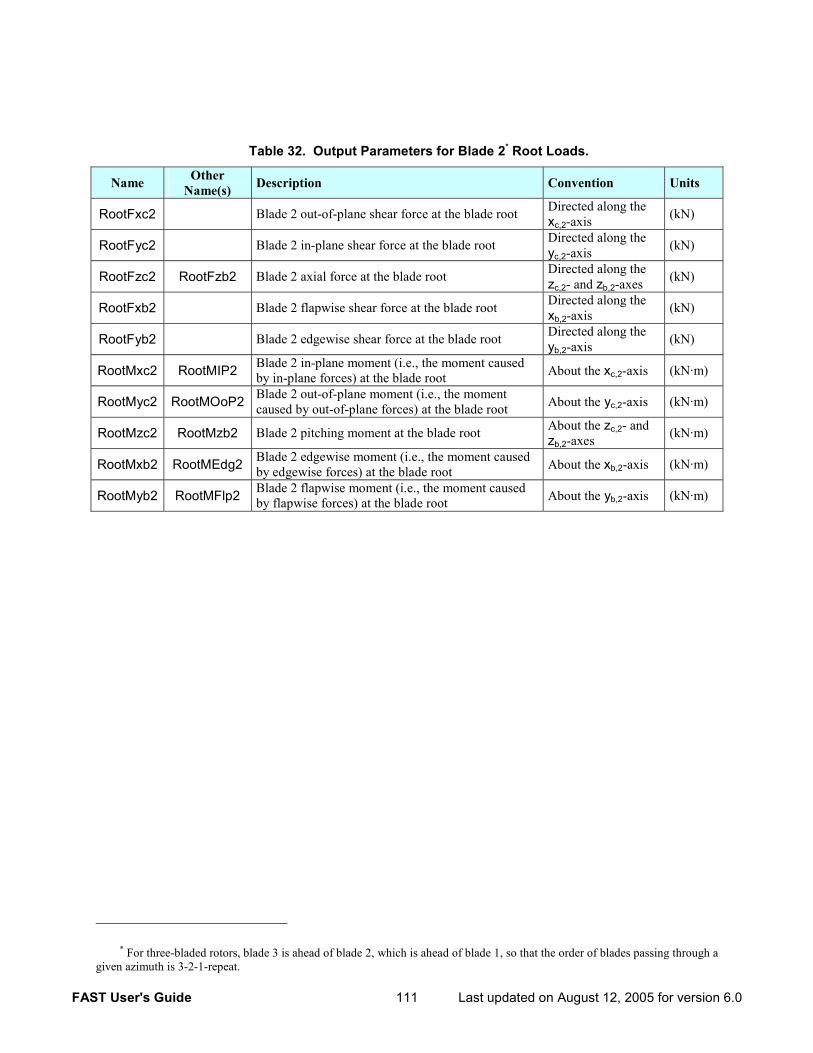
FAST User's Guide 111 Last updated on August 12, 2005 for version 6.0
Table 32. Output Parameters for Blade 2* Root Loads.
Name Other Name(s) Description Convention Units
RootFxc2 Blade 2 out-of-plane shear force at the blade root Directed along the xc,2-axis (kN)
RootFyc2 Blade 2 in-plane shear force at the blade root Directed along the yc,2-axis (kN)
RootFzc2 RootFzb2 Blade 2 axial force at the blade root Directed along the zc,2- and zb,2-axes (kN)
RootFxb2 Blade 2 flapwise shear force at the blade root Directed along the xb,2-axis (kN)
RootFyb2 Blade 2 edgewise shear force at the blade root Directed along the yb,2-axis (kN)
RootMxc2 RootMIP2 Blade 2 in-plane moment (i.e., the moment caused by in-plane forces) at the blade root About the xc,2-axis (kN·m)
RootMyc2 RootMOoP2 Blade 2 out-of-plane moment (i.e., the moment caused by out-of-plane forces) at the blade root About the yc,2-axis (kN·m)
RootMzc2 RootMzb2 Blade 2 pitching moment at the blade root About the zc,2- and zb,2-axes (kN·m)
RootMxb2 RootMEdg2 Blade 2 edgewise moment (i.e., the moment caused by edgewise forces) at the blade root About the xb,2-axis (kN·m)
RootMyb2 RootMFlp2 Blade 2 flapwise moment (i.e., the moment caused by flapwise forces) at the blade root About the yb,2-axis (kN·m)
* For three-bladed rotors, blade 3 is ahead of blade 2, which is ahead of blade 1, so that the order of blades passing through a given azimuth is 3-2-1-repeat.
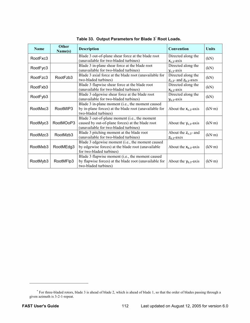
FAST User's Guide 112 Last updated on August 12, 2005 for version 6.0
Table 33. Output Parameters for Blade 3* Root Loads.
Name Other Name(s) Description Convention Units
RootFxc3 Blade 3 out-of-plane shear force at the blade root (unavailable for two-bladed turbines)
Directed along the xc,3-axis (kN)
RootFyc3 Blade 3 in-plane shear force at the blade root (unavailable for two-bladed turbines)
Directed along the yc,3-axis (kN)
RootFzc3 RootFzb3 Blade 3 axial force at the blade root (unavailable for two-bladed turbines)
Directed along the zc,3- and zb,3-axes (kN)
RootFxb3 Blade 3 flapwise shear force at the blade root (unavailable for two-bladed turbines)
Directed along the xb,3-axis (kN)
RootFyb3 Blade 3 edgewise shear force at the blade root (unavailable for two-bladed turbines)
Directed along the yb,3-axis (kN)
RootMxc3 RootMIP3 Blade 3 in-plane moment (i.e., the moment caused by in-plane forces) at the blade root (unavailable for two-bladed turbines)
About the xc,3-axis (kN·m)
RootMyc3 RootMOoP3Blade 3 out-of-plane moment (i.e., the moment caused by out-of-plane forces) at the blade root (unavailable for two-bladed turbines)
About the yc,3-axis (kN·m)
RootMzc3 RootMzb3 Blade 3 pitching moment at the blade root (unavailable for two-bladed turbines)
About the zc,3- and zb,3-axes (kN·m)
RootMxb3 RootMEdg3 Blade 3 edgewise moment (i.e., the moment caused by edgewise forces) at the blade root (unavailable for two-bladed turbines)
About the xb,3-axis (kN·m)
RootMyb3 RootMFlp3 Blade 3 flapwise moment (i.e., the moment caused by flapwise forces) at the blade root (unavailable for two-bladed turbines)
About the yb,3-axis (kN·m)
* For three-bladed rotors, blade 3 is ahead of blade 2, which is ahead of blade 1, so that the order of blades passing through a given azimuth is 3-2-1-repeat.
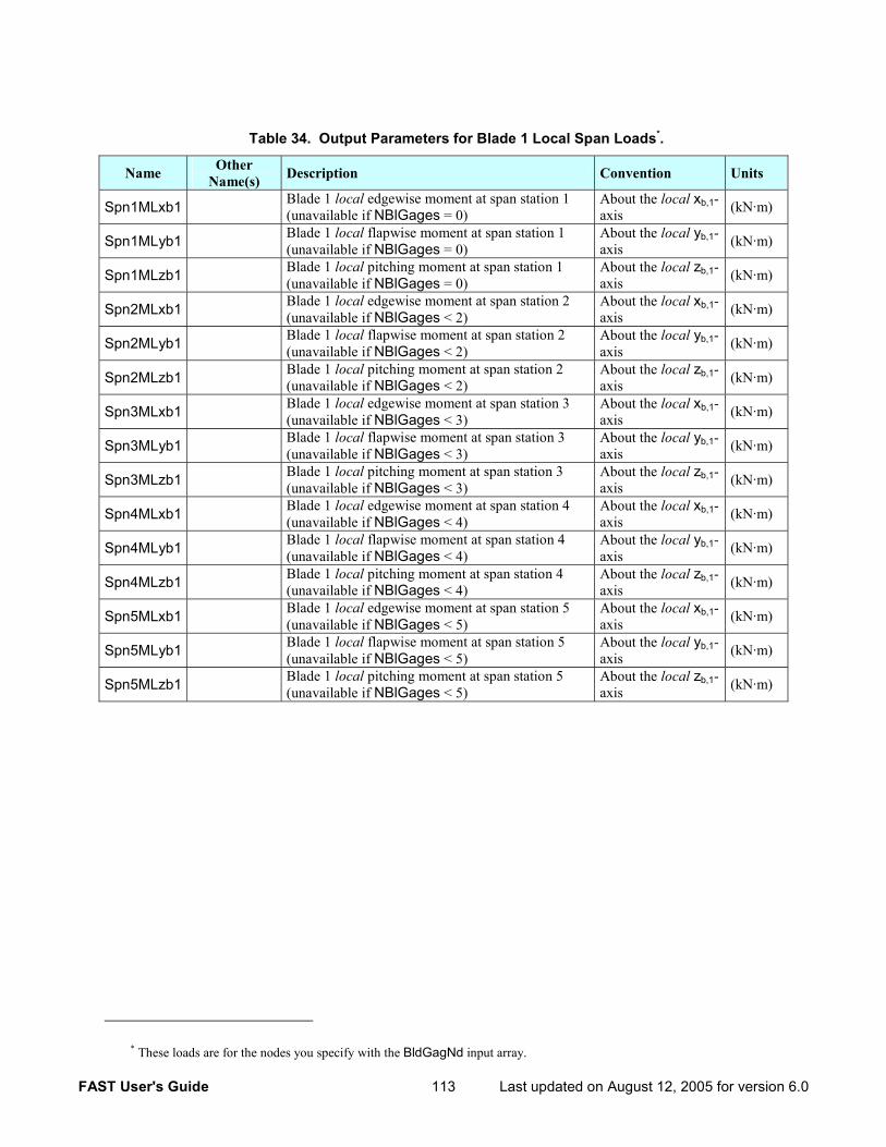
FAST User's Guide 113 Last updated on August 12, 2005 for version 6.0
Table 34. Output Parameters for Blade 1 Local Span Loads*.
Name Other Name(s) Description Convention Units
Spn1MLxb1 Blade 1 local edgewise moment at span station 1 (unavailable if NBlGages = 0)
About the local xb,1-axis (kN·m)
Spn1MLyb1 Blade 1 local flapwise moment at span station 1 (unavailable if NBlGages = 0)
About the local yb,1-axis (kN·m)
Spn1MLzb1 Blade 1 local pitching moment at span station 1 (unavailable if NBlGages = 0)
About the local zb,1-axis (kN·m)
Spn2MLxb1 Blade 1 local edgewise moment at span station 2 (unavailable if NBlGages < 2)
About the local xb,1-axis (kN·m)
Spn2MLyb1 Blade 1 local flapwise moment at span station 2 (unavailable if NBlGages < 2)
About the local yb,1-axis (kN·m)
Spn2MLzb1 Blade 1 local pitching moment at span station 2 (unavailable if NBlGages < 2)
About the local zb,1-axis (kN·m)
Spn3MLxb1 Blade 1 local edgewise moment at span station 3 (unavailable if NBlGages < 3)
About the local xb,1-axis (kN·m)
Spn3MLyb1 Blade 1 local flapwise moment at span station 3 (unavailable if NBlGages < 3)
About the local yb,1-axis (kN·m)
Spn3MLzb1 Blade 1 local pitching moment at span station 3 (unavailable if NBlGages < 3)
About the local zb,1-axis (kN·m)
Spn4MLxb1 Blade 1 local edgewise moment at span station 4 (unavailable if NBlGages < 4)
About the local xb,1-axis (kN·m)
Spn4MLyb1 Blade 1 local flapwise moment at span station 4 (unavailable if NBlGages < 4)
About the local yb,1-axis (kN·m)
Spn4MLzb1 Blade 1 local pitching moment at span station 4 (unavailable if NBlGages < 4)
About the local zb,1-axis (kN·m)
Spn5MLxb1 Blade 1 local edgewise moment at span station 5 (unavailable if NBlGages < 5)
About the local xb,1-axis (kN·m)
Spn5MLyb1 Blade 1 local flapwise moment at span station 5 (unavailable if NBlGages < 5)
About the local yb,1-axis (kN·m)
Spn5MLzb1 Blade 1 local pitching moment at span station 5 (unavailable if NBlGages < 5)
About the local zb,1-axis (kN·m)
* These loads are for the nodes you specify with the BldGagNd input array.
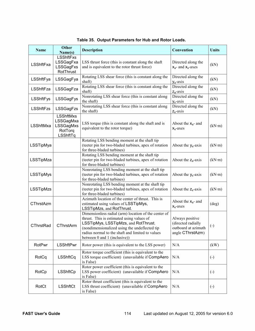
FAST User's Guide 114 Last updated on August 12, 2005 for version 6.0
Table 35. Output Parameters for Hub and Rotor Loads.
Name Other Name(s) Description Convention Units
LSShftFxa
LSShftFxs LSSGagFxa LSSGagFxs RotThrust
LSS thrust force (this is constant along the shaft and is equivalent to the rotor thrust force)
Directed along the xa- and xs-axes (kN)
LSShftFya LSSGagFya Rotating LSS shear force (this is constant along the shaft)
Directed along the ya-axis (kN)
LSShftFza LSSGagFza Rotating LSS shear force (this is constant along the shaft)
Directed along the za-axis (kN)
LSShftFys LSSGagFys Nonrotating LSS shear force (this is constant along the shaft)
Directed along the ys-axis (kN)
LSShftFzs LSSGagFzs Nonrotating LSS shear force (this is constant along the shaft)
Directed along the zs-axis (kN)
LSShftMxa
LSShftMxs LSSGagMxa LSSGagMxs
RotTorq LSShftTq
LSS torque (this is constant along the shaft and is equivalent to the rotor torque)
About the xa- and xs-axes (kN·m)
LSSTipMya Rotating LSS bending moment at the shaft tip (teeter pin for two-bladed turbines, apex of rotation for three-bladed turbines)
About the ya-axis (kN·m)
LSSTipMza Rotating LSS bending moment at the shaft tip (teeter pin for two-bladed turbines, apex of rotation for three-bladed turbines)
About the za-axis (kN·m)
LSSTipMys Nonrotating LSS bending moment at the shaft tip (teeter pin for two-bladed turbines, apex of rotation for three-bladed turbines)
About the ys-axis (kN·m)
LSSTipMzs Nonrotating LSS bending moment at the shaft tip (teeter pin for two-bladed turbines, apex of rotation for three-bladed turbines)
About the zs-axis (kN·m)
CThrstAzm Azimuth location of the center of thrust. This is estimated using values of LSSTipMys, LSSTipMzs, and RotThrust.
About the xa- and xs-axes (deg)
CThrstRad CThrstArm
Dimensionless radial (arm) location of the center of thrust. This is estimated using values of LSSTipMys, LSSTipMzs, and RotThrust. (nondimensionalized using the undeflected tip radius normal to the shaft and limited to values between 0 and 1 (inclusive))
Always positive (directed radially outboard at azimuth angle CThrstAzm)
(-)
RotPwr LSShftPwr Rotor power (this is equivalent to the LSS power) N/A (kW)
RotCq LSShftCq Rotor torque coefficient (this is equivalent to the LSS torque coefficient) (unavailable if CompAero
is False) N/A (-)
RotCp LSShftCp Rotor power coefficient (this is equivalent to the LSS power coefficient) (unavailable if CompAero
is False) N/A (-)
RotCt LSShftCt Rotor thrust coefficient (this is equivalent to the LSS thrust coefficient) (unavailable if CompAero
is False) N/A (-)
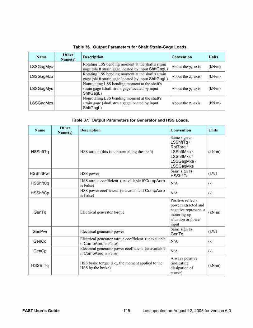
FAST User's Guide 115 Last updated on August 12, 2005 for version 6.0
Table 36. Output Parameters for Shaft Strain-Gage Loads.
Name Other Name(s) Description Convention Units
LSSGagMya Rotating LSS bending moment at the shaft's strain gage (shaft strain gage located by input ShftGagL) About the ya-axis (kN·m)
LSSGagMza Rotating LSS bending moment at the shaft's strain gage (shaft strain gage located by input ShftGagL) About the za-axis (kN·m)
LSSGagMys Nonrotating LSS bending moment at the shaft's strain gage (shaft strain gage located by input ShftGagL)
About the ys-axis (kN·m)
LSSGagMzs Nonrotating LSS bending moment at the shaft's strain gage (shaft strain gage located by input ShftGagL)
About the zs-axis (kN·m)
Table 37. Output Parameters for Generator and HSS Loads.
Name Other Name(s) Description Convention Units
HSShftTq HSS torque (this is constant along the shaft)
Same sign as LSShftTq / RotTorq / LSShftMxa / LSShftMxs / LSSGagMxa / LSSGagMxs
(kN·m)
HSShftPwr HSS power Same sign as HSShftTq (kW)
HSShftCq HSS torque coefficient (unavailable if CompAero is False) N/A (-)
HSShftCp HSS power coefficient (unavailable if CompAero is False) N/A (-)
GenTq Electrical generator torque
Positive reflects power extracted and negative represents a motoring-up situation or power input
(kN·m)
GenPwr Electrical generator power Same sign as GenTq (kW)
GenCq Electrical generator torque coefficient (unavailable if CompAero is False) N/A (-)
GenCp Electrical generator power coefficient (unavailable if CompAero is False) N/A (-)
HSSBrTq HSS brake torque (i.e., the moment applied to the HSS by the brake)
Always positive (indicating dissipation of power)
(kN·m)
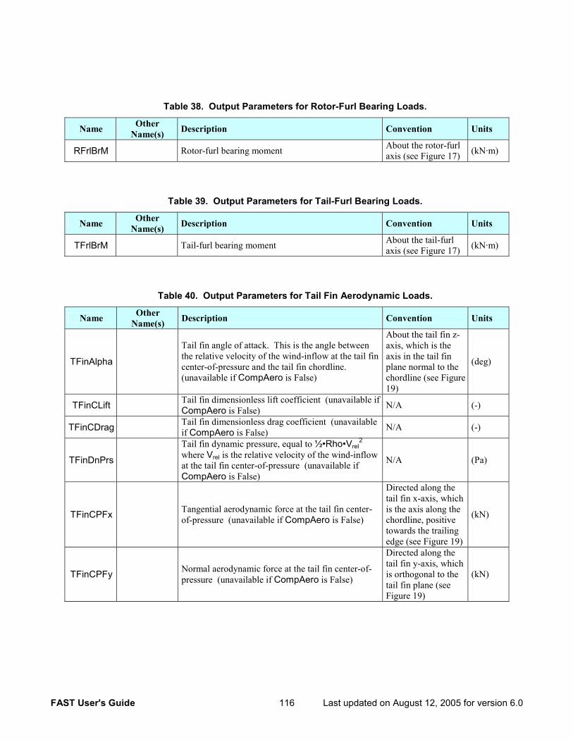
FAST User's Guide 116 Last updated on August 12, 2005 for version 6.0
Table 38. Output Parameters for Rotor-Furl Bearing Loads.
Name Other Name(s) Description Convention Units
RFrlBrM Rotor-furl bearing moment About the rotor-furl axis (see Figure 17) (kN·m)
Table 39. Output Parameters for Tail-Furl Bearing Loads.
Name Other Name(s) Description Convention Units
TFrlBrM Tail-furl bearing moment About the tail-furl axis (see Figure 17) (kN·m)
Table 40. Output Parameters for Tail Fin Aerodynamic Loads.
Name Other Name(s) Description Convention Units
TFinAlpha
Tail fin angle of attack. This is the angle between the relative velocity of the wind-inflow at the tail fin center-of-pressure and the tail fin chordline. (unavailable if CompAero is False)
About the tail fin z-axis, which is the axis in the tail fin plane normal to the chordline (see Figure 19)
(deg)
TFinCLift Tail fin dimensionless lift coefficient (unavailable if CompAero is False) N/A (-)
TFinCDrag Tail fin dimensionless drag coefficient (unavailable if CompAero is False) N/A (-)
TFinDnPrs
Tail fin dynamic pressure, equal to ½•Rho•Vrel2
where Vrel is the relative velocity of the wind-inflow at the tail fin center-of-pressure (unavailable if CompAero is False)
N/A (Pa)
TFinCPFx Tangential aerodynamic force at the tail fin center-of-pressure (unavailable if CompAero is False)
Directed along the tail fin x-axis, which is the axis along the chordline, positive towards the trailing edge (see Figure 19)
(kN)
TFinCPFy Normal aerodynamic force at the tail fin center-of-pressure (unavailable if CompAero is False)
Directed along the tail fin y-axis, which is orthogonal to the tail fin plane (see Figure 19)
(kN)

FAST User's Guide 117 Last updated on August 12, 2005 for version 6.0
Table 41. Output Parameters for Tower-Top, Yaw-Bearing Loads.
Name Other Name(s) Description Convention Units
YawBrFxn Rotating (with nacelle) tower-top / yaw bearing shear force
Directed along the xn-axis (kN)
YawBrFyn Rotating (with nacelle) tower-top / yaw bearing shear force
Directed along the yn-axis (kN)
YawBrFzn YawBrFzp Tower-top / yaw bearing axial force Directed along the zn- and zp-axes (kN)
YawBrFxp Tower-top / yaw bearing fore-aft (nonrotating) shear force
Directed along the xp-axis (kN)
YawBrFyp Tower-top / yaw bearing side-to-side (nonrotating) shear force
Directed along the yp-axis (kN)
YawBrMxn Rotating (with nacelle) tower-top / yaw bearing roll moment About the xn-axis (kN·m)
YawBrMyn Rotating (with nacelle) tower-top / yaw bearing pitch moment About the yn-axis (kN·m)
YawBrMzn YawBrMzp YawMom Tower-top / yaw bearing yaw moment About the zn- and
zp-axes (kN·m)
YawBrMxp Nonrotating tower-top / yaw bearing roll moment About the xp-axis (kN·m)
YawBrMyp Nonrotating tower-top / yaw bearing pitch moment About the yp-axis (kN·m)
Table 42. Output Parameters for Tower Base Loads.
Name Other Name(s) Description Convention Units
TwrBsFxt Tower base fore-aft shear force Directed along the xt-axis (kN)
TwrBsFyt Tower base side-to-side shear force Directed along the yt-axis (kN)
TwrBsFzt Tower base axial force Directed along the zt-axis (kN)
TwrBsMxt Tower base roll (or side-to-side) moment (i.e., the moment caused by side-to-side forces) About the xt-axis (kN·m)
TwrBsMyt Tower base pitching (or fore-aft) moment (i.e., the moment caused by fore-aft forces) About the yt-axis (kN·m)
TwrBsMzt Tower base yaw (or torsional) moment About the zt-axis (kN·m)
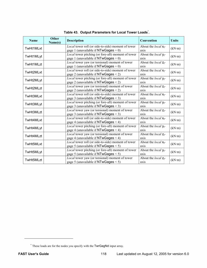
FAST User's Guide 118 Last updated on August 12, 2005 for version 6.0
Table 43. Output Parameters for Local Tower Loads*.
Name Other Name(s) Description Convention Units
TwHt1MLxt Local tower roll (or side-to-side) moment of tower gage 1 (unavailable if NTwGages = 0)
About the local xt-axis (kN·m)
TwHt1MLyt Local tower pitching (or fore-aft) moment of tower gage 1 (unavailable if NTwGages = 0)
About the local yt-axis (kN·m)
TwHt1MLzt Local tower yaw (or torsional) moment of tower gage 1 (unavailable if NTwGages = 0)
About the local zt-axis (kN·m)
TwHt2MLxt Local tower roll (or side-to-side) moment of tower gage 2 (unavailable if NTwGages < 2)
About the local xt-axis (kN·m)
TwHt2MLyt Local tower pitching (or fore-aft) moment of tower gage 2 (unavailable if NTwGages < 2)
About the local yt-axis (kN·m)
TwHt2MLzt Local tower yaw (or torsional) moment of tower gage 2 (unavailable if NTwGages < 2)
About the local zt-axis (kN·m)
TwHt3MLxt Local tower roll (or side-to-side) moment of tower gage 3 (unavailable if NTwGages < 3)
About the local xt-axis (kN·m)
TwHt3MLyt Local tower pitching (or fore-aft) moment of tower gage 3 (unavailable if NTwGages < 3)
About the local yt-axis (kN·m)
TwHt3MLzt Local tower yaw (or torsional) moment of tower gage 3 (unavailable if NTwGages < 3)
About the local zt-axis (kN·m)
TwHt4MLxt Local tower roll (or side-to-side) moment of tower gage 4 (unavailable if NTwGages < 4)
About the local xt-axis (kN·m)
TwHt4MLyt Local tower pitching (or fore-aft) moment of tower gage 4 (unavailable if NTwGages < 4)
About the local yt-axis (kN·m)
TwHt4MLzt Local tower yaw (or torsional) moment of tower gage 4 (unavailable if NTwGages < 4)
About the local zt-axis (kN·m)
TwHt5MLxt Local tower roll (or side-to-side) moment of tower gage 5 (unavailable if NTwGages < 5)
About the local xt-axis (kN·m)
TwHt5MLyt Local tower pitching (or fore-aft) moment of tower gage 5 (unavailable if NTwGages < 5)
About the local yt-axis (kN·m)
TwHt5MLzt Local tower yaw (or torsional) moment of tower gage 5 (unavailable if NTwGages < 5)
About the local zt-axis (kN·m)
* These loads are for the nodes you specify with the TwrGagNd input array.
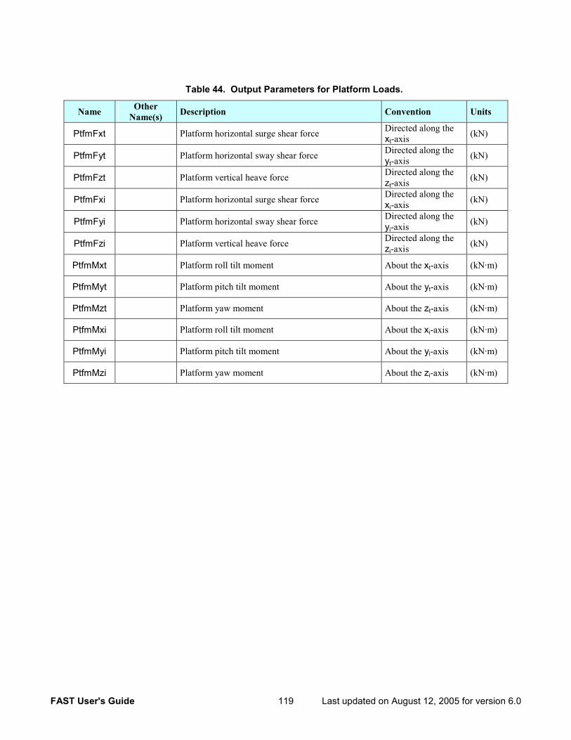
FAST User's Guide 119 Last updated on August 12, 2005 for version 6.0
Table 44. Output Parameters for Platform Loads.
Name Other Name(s) Description Convention Units
PtfmFxt Platform horizontal surge shear force Directed along the xt-axis (kN)
PtfmFyt Platform horizontal sway shear force Directed along the yt-axis (kN)
PtfmFzt Platform vertical heave force Directed along the zt-axis (kN)
PtfmFxi Platform horizontal surge shear force Directed along the xi-axis (kN)
PtfmFyi Platform horizontal sway shear force Directed along the yi-axis (kN)
PtfmFzi Platform vertical heave force Directed along the zi-axis (kN)
PtfmMxt Platform roll tilt moment About the xt-axis (kN·m)
PtfmMyt Platform pitch tilt moment About the yt-axis (kN·m)
PtfmMzt Platform yaw moment About the zt-axis (kN·m)
PtfmMxi Platform roll tilt moment About the xi-axis (kN·m)
PtfmMyi Platform pitch tilt moment About the yi-axis (kN·m)
PtfmMzi Platform yaw moment About the zi-axis (kN·m)
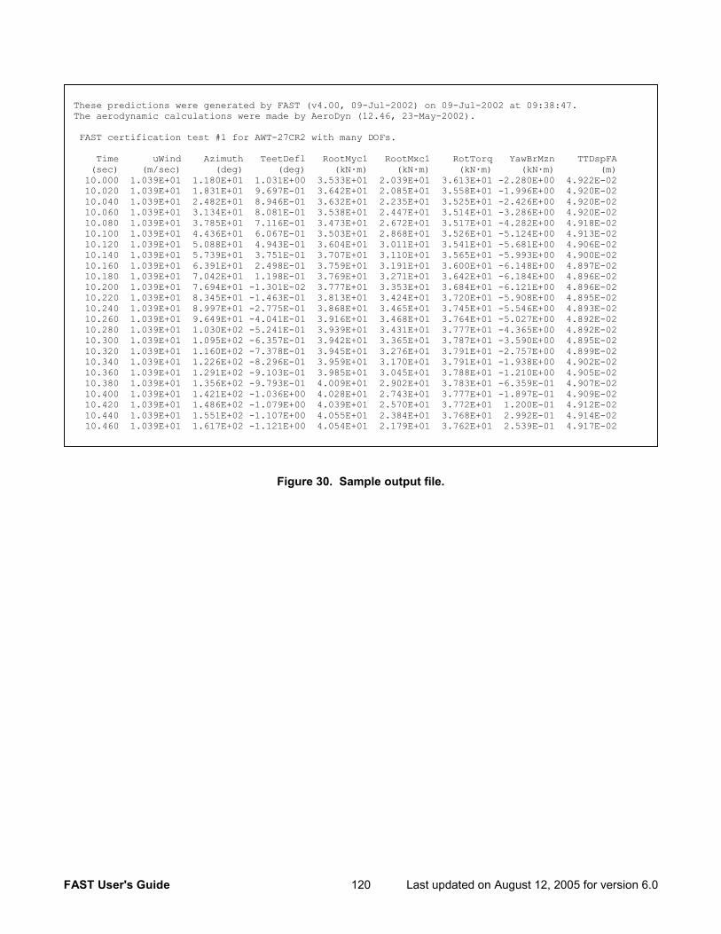
FAST User's Guide 120 Last updated on August 12, 2005 for version 6.0
Figure 30. Sample output file.
These predictions were generated by FAST (v4.00, 09-Jul-2002) on 09-Jul-2002 at 09:38:47. The aerodynamic calculations were made by AeroDyn (12.46, 23-May-2002). FAST certification test #1 for AWT-27CR2 with many DOFs. Time uWind Azimuth TeetDefl RootMyc1 RootMxc1 RotTorq YawBrMzn TTDspFA (sec) (m/sec) (deg) (deg) (kN·m) (kN·m) (kN·m) (kN·m) (m) 10.000 1.039E+01 1.180E+01 1.031E+00 3.533E+01 2.039E+01 3.613E+01 -2.280E+00 4.922E-02 10.020 1.039E+01 1.831E+01 9.697E-01 3.642E+01 2.085E+01 3.558E+01 -1.996E+00 4.920E-02 10.040 1.039E+01 2.482E+01 8.946E-01 3.632E+01 2.235E+01 3.525E+01 -2.426E+00 4.920E-02 10.060 1.039E+01 3.134E+01 8.081E-01 3.538E+01 2.447E+01 3.514E+01 -3.286E+00 4.920E-02 10.080 1.039E+01 3.785E+01 7.116E-01 3.473E+01 2.672E+01 3.517E+01 -4.282E+00 4.918E-02 10.100 1.039E+01 4.436E+01 6.067E-01 3.503E+01 2.868E+01 3.526E+01 -5.124E+00 4.913E-02 10.120 1.039E+01 5.088E+01 4.943E-01 3.604E+01 3.011E+01 3.541E+01 -5.681E+00 4.906E-02 10.140 1.039E+01 5.739E+01 3.751E-01 3.707E+01 3.110E+01 3.565E+01 -5.993E+00 4.900E-02 10.160 1.039E+01 6.391E+01 2.498E-01 3.759E+01 3.191E+01 3.600E+01 -6.148E+00 4.897E-02 10.180 1.039E+01 7.042E+01 1.198E-01 3.769E+01 3.271E+01 3.642E+01 -6.184E+00 4.896E-02 10.200 1.039E+01 7.694E+01 -1.301E-02 3.777E+01 3.353E+01 3.684E+01 -6.121E+00 4.896E-02 10.220 1.039E+01 8.345E+01 -1.463E-01 3.813E+01 3.424E+01 3.720E+01 -5.908E+00 4.895E-02 10.240 1.039E+01 8.997E+01 -2.775E-01 3.868E+01 3.465E+01 3.745E+01 -5.546E+00 4.893E-02 10.260 1.039E+01 9.649E+01 -4.041E-01 3.916E+01 3.468E+01 3.764E+01 -5.027E+00 4.892E-02 10.280 1.039E+01 1.030E+02 -5.241E-01 3.939E+01 3.431E+01 3.777E+01 -4.365E+00 4.892E-02 10.300 1.039E+01 1.095E+02 -6.357E-01 3.942E+01 3.365E+01 3.787E+01 -3.590E+00 4.895E-02 10.320 1.039E+01 1.160E+02 -7.378E-01 3.945E+01 3.276E+01 3.791E+01 -2.757E+00 4.899E-02 10.340 1.039E+01 1.226E+02 -8.296E-01 3.959E+01 3.170E+01 3.791E+01 -1.938E+00 4.902E-02 10.360 1.039E+01 1.291E+02 -9.103E-01 3.985E+01 3.045E+01 3.788E+01 -1.210E+00 4.905E-02 10.380 1.039E+01 1.356E+02 -9.793E-01 4.009E+01 2.902E+01 3.783E+01 -6.359E-01 4.907E-02 10.400 1.039E+01 1.421E+02 -1.036E+00 4.028E+01 2.743E+01 3.777E+01 -1.897E-01 4.909E-02 10.420 1.039E+01 1.486E+02 -1.079E+00 4.039E+01 2.570E+01 3.772E+01 1.200E-01 4.912E-02 10.440 1.039E+01 1.551E+02 -1.107E+00 4.055E+01 2.384E+01 3.768E+01 2.992E-01 4.914E-02
10.460 1.039E+01 1.617E+02 -1.121E+00 4.054E+01 2.179E+01 3.762E+01 2.539E-01 4.917E-02
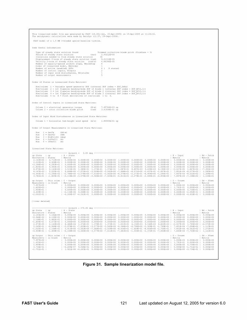
FAST User's Guide 121 Last updated on August 12, 2005 for version 6.0
Figure 31. Sample linearization model file.
This linearized model file was generated by FAST (v6.00c-jmj, 15-Apr-2005) on 15-Apr-2005 at 11:24:16. The aerodynamic calculations were made by AeroDyn (12.57, 29-Sept-2004). FAST model of a 1.5 MW 3-bladed upwind baseline turbine. Some Useful Information: Type of steady state solution found Trimmed collective blade pitch (TrimCase = 3) Period of steady state solution (sec) 2.93212E+00 Iterations needed to find steady state solution 34 Displacement 2-norm of steady state solution (rad) 9.01316E-05 Velocity 2-norm of steady state solution (rad/s) 4.84390E-05 Number of equally-speced azimuth steps, NAzimStep 4 Order of linearized model, MdlOrder 1 Number of active (enabled) DOFs 4 ( 8 states) Number of control inputs, NInputs 2 Number of input wind disturbances, NDisturbs 1 Number of output measurements 5 Order of States in Linearized State Matrices: Row/column 1 = Variable speed generator DOF (internal DOF index = DOF_GeAz) Row/column 2 = 1st flapwise bending-mode DOF of blade 1 (internal DOF index = DOF_BF(1,1)) Row/column 3 = 1st flapwise bending-mode DOF of blade 2 (internal DOF index = DOF_BF(2,1)) Row/column 4 = 1st flapwise bending-mode DOF of blade 3 (internal DOF index = DOF_BF(3,1)) Row/column 5 to 8 = First derivatives of row/column 1 to 4. Order of Control Inputs in Linearized State Matrices: Column 1 = electrical generator torque (N·m) 7.95744E+03 op Column 2 = rotor collective blade pitch (rad) 3.41938E-01 op Order of Input Wind Disturbances in Linearized State Matrices: Column 1 = horizontal hub-height wind speed (m/s) 1.80000E+01 op Order of Output Measurements in Linearized State Matrices: Row 1 = GenTq (kN·m) Row 2 = GenPwr (kW) Row 3 = BldPitch1 (deg) Row 4 = OoPDefl1 (m) Row 5 = IPDefl1 (m) Linearized State Matrices: ----------------------------- Azimuth = 0.00 deg ----------------------------- op State | op | A - State | B - Input | Bd - DstrbDerivativs | States | Matrix | Matrix | Matrix 2.143E+00 | 4.712E+00 | 0.000E+00 0.000E+00 0.000E+00 0.000E+00 1.000E+00 0.000E+00 0.000E+00 0.000E+00 | 0.000E+00 0.000E+00 | 0.000E+00 2.222E-01 | 4.928E-01 | 0.000E+00 0.000E+00 0.000E+00 0.000E+00 0.000E+00 1.000E+00 0.000E+00 0.000E+00 | 0.000E+00 0.000E+00 | 0.000E+00-3.294E-02 | 6.283E-01 | 0.000E+00 0.000E+00 0.000E+00 0.000E+00 0.000E+00 0.000E+00 1.000E+00 0.000E+00 | 0.000E+00 0.000E+00 | 0.000E+00-1.825E-01 | 4.442E-01 | 0.000E+00 0.000E+00 0.000E+00 0.000E+00 0.000E+00 0.000E+00 0.000E+00 1.000E+00 | 0.000E+00 0.000E+00 | 0.000E+00 8.973E-05 | 2.143E+00 | 3.515E-05 1.380E-01 1.373E-01 1.374E-01 1.087E-01 8.897E-03 9.439E-03 6.190E-03 | -3.027E-05 1.867E+00 | -7.305E-03 8.147E-03 | 2.222E-01 | 6.668E+00 -7.072E+01 -3.559E+00 -3.562E+00 -7.968E+01 -8.571E+00 -2.437E-01 -1.607E-01 | 7.851E-04 -8.277E+02 | 1.282E+01-4.493E-01 | -3.294E-02 | -2.788E+00 -3.578E+00 -7.014E+01 -3.563E+00 -8.379E+01 -2.273E-01 -8.909E+00 -1.590E-01 | 7.847E-04 -8.522E+02 | 1.308E+01 3.781E-01 | -1.825E-01 | -4.118E+00 -3.579E+00 -3.560E+00 -7.020E+01 -6.411E+01 -2.279E-01 -2.445E-01 -6.834E+00 | 7.847E-04 -7.148E+02 | 1.124E+01 op Output | This colmn | C - Output | D - Trnsmt | Dd - DTsmtMeasurmnts | is blank | Matrix | Matrix | Matrix 7.957E+00 | | 0.000E+00 0.000E+00 0.000E+00 0.000E+00 0.000E+00 0.000E+00 0.000E+00 0.000E+00 | 1.000E-03 0.000E+00 | 0.000E+00 1.425E+03 | | 0.000E+00 0.000E+00 0.000E+00 0.000E+00 6.650E+02 0.000E+00 0.000E+00 0.000E+00 | 1.791E-01 0.000E+00 | 0.000E+00 1.959E+01 | | 0.000E+00 0.000E+00 0.000E+00 0.000E+00 0.000E+00 0.000E+00 0.000E+00 0.000E+00 | 0.000E+00 5.730E+01 | 0.000E+00 4.459E-01 | | -2.134E-06 9.048E-01 0.000E+00 0.000E+00 0.000E+00 0.000E+00 0.000E+00 0.000E+00 | 0.000E+00 -2.092E-01 | 0.000E+00-2.091E-01 | | -4.269E-07 -4.243E-01 0.000E+00 0.000E+00 0.000E+00 0.000E+00 0.000E+00 0.000E+00 | 0.000E+00 -4.459E-01 | 0.000E+00 [lines deleted] ----------------------------- Azimuth = 270.00 deg ----------------------------- op State | op | A - State | B - Input | Bd - DstrbDerivativs | States | Matrix | Matrix | Matrix 2.143E+00 | 3.142E+00 | 0.000E+00 0.000E+00 0.000E+00 0.000E+00 1.000E+00 0.000E+00 0.000E+00 0.000E+00 | 0.000E+00 0.000E+00 | 0.000E+00-6.944E-02 | 4.126E-01 | 0.000E+00 0.000E+00 0.000E+00 0.000E+00 0.000E+00 1.000E+00 0.000E+00 0.000E+00 | 0.000E+00 0.000E+00 | 0.000E+00 2.108E-01 | 5.462E-01 | 0.000E+00 0.000E+00 0.000E+00 0.000E+00 0.000E+00 0.000E+00 1.000E+00 0.000E+00 | 0.000E+00 0.000E+00 | 0.000E+00-1.409E-01 | 6.073E-01 | 0.000E+00 0.000E+00 0.000E+00 0.000E+00 0.000E+00 0.000E+00 0.000E+00 1.000E+00 | 0.000E+00 0.000E+00 | 0.000E+00 2.973E-05 | 2.143E+00 | 8.486E-04 1.374E-01 1.379E-01 1.373E-01 1.021E-01 6.150E-03 9.160E-03 6.822E-03 | -3.027E-05 1.795E+00 | -4.572E-03 5.245E-01 | -6.944E-02 | -3.978E-01 -7.029E+01 -3.577E+00 -3.560E+00 -6.344E+01 -6.790E+00 -2.369E-01 -1.769E-01 | 7.851E-04 -7.094E+02 | 1.113E+01-1.025E-01 | 2.108E-01 | 5.913E+00 -3.563E+00 -7.069E+01 -3.559E+00 -8.454E+01 -1.609E-01 -8.656E+00 -1.756E-01 | 7.852E-04 -8.561E+02 | 1.272E+01-4.959E-01 | -1.409E-01 | -6.108E+00 -3.565E+00 -3.577E+00 -7.011E+01 -7.481E+01 -1.555E-01 -2.372E-01 -7.050E+00 | 7.845E-04 -7.755E+02 | 1.121E+01 op Output | This colmn | C - Output | D - Trnsmt | Dd - DTsmtMeasurmnts | is blank | Matrix | Matrix | Matrix 7.957E+00 | | 0.000E+00 0.000E+00 0.000E+00 0.000E+00 0.000E+00 0.000E+00 0.000E+00 0.000E+00 | 1.000E-03 0.000E+00 | 0.000E+00 1.425E+03 | | 0.000E+00 0.000E+00 0.000E+00 0.000E+00 6.650E+02 0.000E+00 0.000E+00 0.000E+00 | 1.791E-01 0.000E+00 | 0.000E+00 1.959E+01 | | 0.000E+00 0.000E+00 0.000E+00 0.000E+00 0.000E+00 0.000E+00 0.000E+00 0.000E+00 | 0.000E+00 5.730E+01 | 0.000E+00 3.734E-01 | | -4.269E-07 9.048E-01 0.000E+00 0.000E+00 0.000E+00 0.000E+00 0.000E+00 0.000E+00 | 0.000E+00 -1.751E-01 | 0.000E+00-1.751E-01 | | 1.921E-06 -4.243E-01 0.000E+00 0.000E+00 0.000E+00 0.000E+00 0.000E+00 0.000E+00 | 0.000E+00 -3.734E-01 | 0.000E+00

FAST User's Guide 122 Last updated on August 12, 2005 for version 6.0
Figure 32. Sample summary file.
This summary information was generated by FAST (v6.00c-jmj, 15-Apr-2005) on 15-Apr-2005 at 16:37:53. FAST certification Test #01: AWT-27CR2 with many DOFs with fixed yaw error and steady wind. Turbine features: Downwind, two-bladed rotor with teetering hub. Rigid foundation. The model has 13 of 22 DOFs active (enabled) at start-up. Enabled First flapwise blade mode DOF. Enabled Second flapwise blade mode DOF. Enabled Edgewise blade mode DOF. Enabled Rotor-teeter DOF. Enabled Drivetrain rotational-flexibility DOF. Enabled Generator DOF. Disabled Rotor-furl DOF. Disabled Tail-furl DOF. Disabled Yaw DOF. Enabled First tower fore-aft bending-mode DOF. Enabled Second tower fore-aft bending-mode DOF. Enabled First tower side-to-side bending-mode DOF. Enabled Second tower side-to-side bending-mode DOF. Disabled Platform horizontal surge translation DOF. Disabled Platform horizontal sway translation DOF. Disabled Platform vertical heave translation DOF. Disabled Platform roll tilt rotation DOF. Disabled Platform pitch tilt rotation DOF. Disabled Platform yaw rotation DOF. Enabled Computation of aerodynamic loads. Disabled Computation of aeroacoustics. Time steps: Structural (s) 0.00400000 Aerodynamic (s) 0.00400000 Some calculated parameters: Hub-Height (m) 42.672 Flexible Tower Length (m) 41.980 Flexible Blade Length (m) 12.573 Rotor mass properties: Rotor Mass (kg) 2200.608 Rotor Inertia (kg-m^2) 41755.996 Blade 1 Blade 2 ------- ------- Mass (kg) 435.304 435.304 Second Mass Moment (kg-m^2) 15434.709 15434.709 First Mass Moment (kg-m) 2120.280 2120.280 Center of Mass (m) 4.871 4.871 Additional mass properties: Tower-top Mass (kg) 7216.038 Tower Mass (kg) 36907.137 Turbine Mass (kg) 44123.176 Mass Incl. Platform (kg) 44123.176
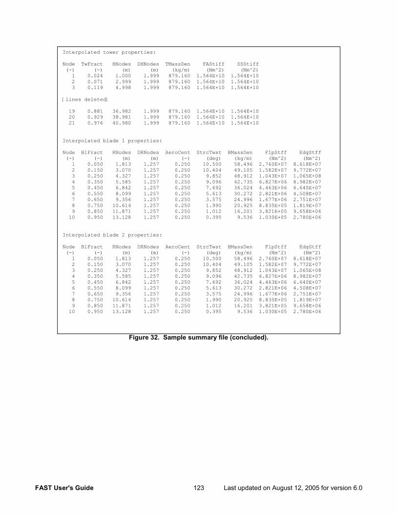
FAST User's Guide 123 Last updated on August 12, 2005 for version 6.0
Figure 32. Sample summary file (concluded).
Interpolated tower properties: Node TwFract HNodes DHNodes TMassDen FAStiff SSStiff (-) (-) (m) (m) (kg/m) (Nm^2) (Nm^2) 1 0.024 1.000 1.999 879.160 1.564E+10 1.564E+10 2 0.071 2.999 1.999 879.160 1.564E+10 1.564E+10 3 0.119 4.998 1.999 879.160 1.564E+10 1.564E+10 [lines deleted] 19 0.881 36.982 1.999 879.160 1.564E+10 1.564E+10 20 0.929 38.981 1.999 879.160 1.564E+10 1.564E+10 21 0.976 40.980 1.999 879.160 1.564E+10 1.564E+10 Interpolated blade 1 properties: Node BlFract RNodes DRNodes AeroCent StrcTwst BMassDen FlpStff EdgStff (-) (-) (m) (m) (-) (deg) (kg/m) (Nm^2) (Nm^2) 1 0.050 1.813 1.257 0.250 10.500 58.496 2.760E+07 8.618E+07 2 0.150 3.070 1.257 0.250 10.404 49.105 1.582E+07 9.772E+07 3 0.250 4.327 1.257 0.250 9.852 48.912 1.043E+07 1.065E+08 4 0.350 5.585 1.257 0.250 9.096 42.735 6.827E+06 8.982E+07 5 0.450 6.842 1.257 0.250 7.692 36.024 4.463E+06 6.640E+07 6 0.550 8.099 1.257 0.250 5.613 30.272 2.821E+06 4.508E+07 7 0.650 9.356 1.257 0.250 3.575 24.996 1.677E+06 2.751E+07 8 0.750 10.614 1.257 0.250 1.990 20.925 8.835E+05 1.819E+07 9 0.850 11.871 1.257 0.250 1.012 16.201 3.821E+05 9.658E+06 10 0.950 13.128 1.257 0.250 0.395 9.536 1.030E+05 2.780E+06 Interpolated blade 2 properties: Node BlFract RNodes DRNodes AeroCent StrcTwst BMassDen FlpStff EdgStff (-) (-) (m) (m) (-) (deg) (kg/m) (Nm^2) (Nm^2) 1 0.050 1.813 1.257 0.250 10.500 58.496 2.760E+07 8.618E+07 2 0.150 3.070 1.257 0.250 10.404 49.105 1.582E+07 9.772E+07 3 0.250 4.327 1.257 0.250 9.852 48.912 1.043E+07 1.065E+08 4 0.350 5.585 1.257 0.250 9.096 42.735 6.827E+06 8.982E+07 5 0.450 6.842 1.257 0.250 7.692 36.024 4.463E+06 6.640E+07 6 0.550 8.099 1.257 0.250 5.613 30.272 2.821E+06 4.508E+07 7 0.650 9.356 1.257 0.250 3.575 24.996 1.677E+06 2.751E+07 8 0.750 10.614 1.257 0.250 1.990 20.925 8.835E+05 1.819E+07 9 0.850 11.871 1.257 0.250 1.012 16.201 3.821E+05 9.658E+06 10 0.950 13.128 1.257 0.250 0.395 9.536 1.030E+05 2.780E+06
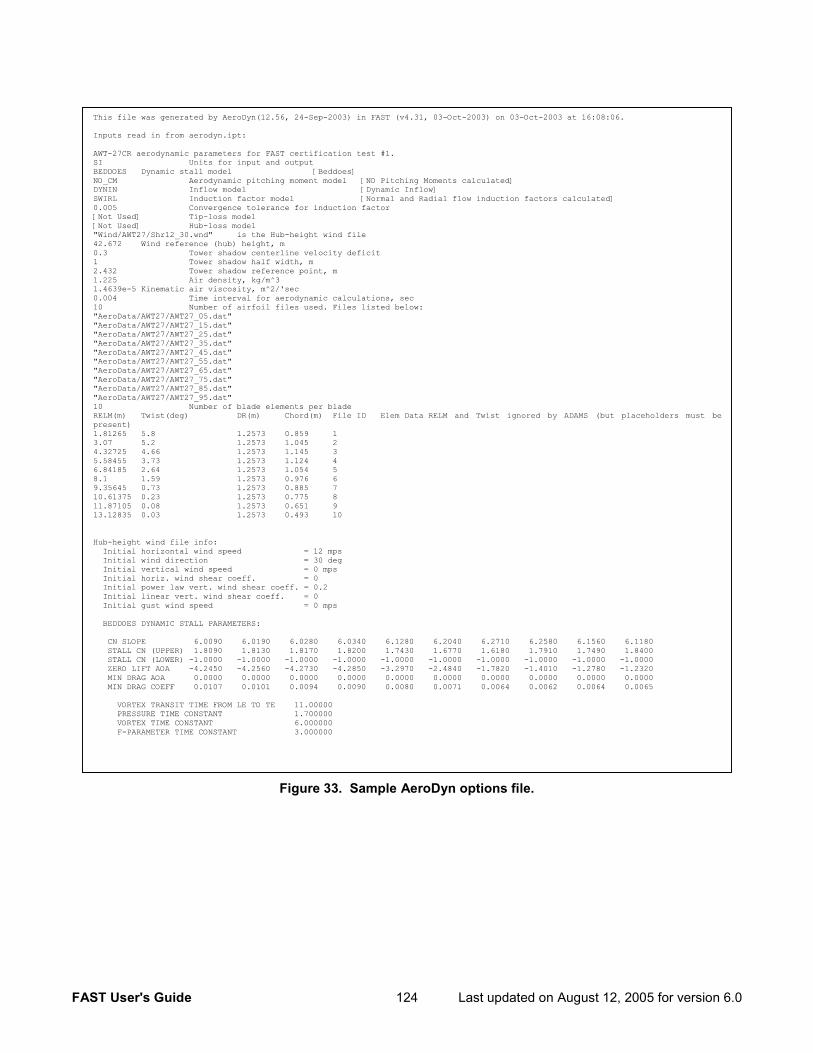
FAST User's Guide 124 Last updated on August 12, 2005 for version 6.0
Figure 33. Sample AeroDyn options file.
This file was generated by AeroDyn(12.56, 24-Sep-2003) in FAST (v4.31, 03-Oct-2003) on 03-Oct-2003 at 16:08:06. Inputs read in from aerodyn.ipt: AWT-27CR aerodynamic parameters for FAST certification test #1. SI Units for input and output BEDDOES Dynamic stall model [Beddoes] NO_CM Aerodynamic pitching moment model [NO Pitching Moments calculated] DYNIN Inflow model [Dynamic Inflow] SWIRL Induction factor model [Normal and Radial flow induction factors calculated] 0.005 Convergence tolerance for induction factor [Not Used] Tip-loss model [Not Used] Hub-loss model "Wind/AWT27/Shr12_30.wnd" is the Hub-height wind file 42.672 Wind reference (hub) height, m 0.3 Tower shadow centerline velocity deficit 1 Tower shadow half width, m 2.432 Tower shadow reference point, m 1.225 Air density, kg/m^3 1.4639e-5 Kinematic air viscosity, m^2/'sec 0.004 Time interval for aerodynamic calculations, sec 10 Number of airfoil files used. Files listed below: "AeroData/AWT27/AWT27_05.dat" "AeroData/AWT27/AWT27_15.dat" "AeroData/AWT27/AWT27_25.dat" "AeroData/AWT27/AWT27_35.dat" "AeroData/AWT27/AWT27_45.dat" "AeroData/AWT27/AWT27_55.dat" "AeroData/AWT27/AWT27_65.dat" "AeroData/AWT27/AWT27_75.dat" "AeroData/AWT27/AWT27_85.dat" "AeroData/AWT27/AWT27_95.dat" 10 Number of blade elements per blade RELM(m) Twist(deg) DR(m) Chord(m) File ID Elem Data RELM and Twist ignored by ADAMS (but placeholders must bepresent) 1.81265 5.8 1.2573 0.859 1 3.07 5.2 1.2573 1.045 2 4.32725 4.66 1.2573 1.145 3 5.58455 3.73 1.2573 1.124 4 6.84185 2.64 1.2573 1.054 5 8.1 1.59 1.2573 0.976 6 9.35645 0.73 1.2573 0.885 7 10.61375 0.23 1.2573 0.775 8 11.87105 0.08 1.2573 0.651 9 13.12835 0.03 1.2573 0.493 10 Hub-height wind file info: Initial horizontal wind speed = 12 mps Initial wind direction = 30 deg Initial vertical wind speed = 0 mps Initial horiz. wind shear coeff. = 0 Initial power law vert. wind shear coeff. = 0.2 Initial linear vert. wind shear coeff. = 0 Initial gust wind speed = 0 mps BEDDOES DYNAMIC STALL PARAMETERS: CN SLOPE 6.0090 6.0190 6.0280 6.0340 6.1280 6.2040 6.2710 6.2580 6.1560 6.1180 STALL CN (UPPER) 1.8090 1.8130 1.8170 1.8200 1.7430 1.6770 1.6180 1.7910 1.7490 1.8400 STALL CN (LOWER) -1.0000 -1.0000 -1.0000 -1.0000 -1.0000 -1.0000 -1.0000 -1.0000 -1.0000 -1.0000 ZERO LIFT AOA -4.2450 -4.2560 -4.2730 -4.2850 -3.2970 -2.4840 -1.7820 -1.4010 -1.2780 -1.2320 MIN DRAG AOA 0.0000 0.0000 0.0000 0.0000 0.0000 0.0000 0.0000 0.0000 0.0000 0.0000 MIN DRAG COEFF 0.0107 0.0101 0.0094 0.0090 0.0080 0.0071 0.0064 0.0062 0.0064 0.0065 VORTEX TRANSIT TIME FROM LE TO TE 11.00000 PRESSURE TIME CONSTANT 1.700000 VORTEX TIME CONSTANT 6.000000 F-PARAMETER TIME CONSTANT 3.000000
FAST User's Guide 125 Last updated on August 12, 2005 for version 6.0
REFERENCES
1. Laino, D.J.; Hansen, A.C. “User’s Guide to the Wind Turbine Dynamics Computer Software AeroDyn.” Salt Lake City, Utah: Windward Engineering, LC, August 2001.
2. Bossanyi, E.A. “GH Bladed Version 3.6 User Manual.” Document 282/BR/010 Issue 12. Garrad Hassan and Partners Limited, 2003.
3. Manjock, A. “Evaluation Report: Design Codes FAST and ADAMS® for Load Calculations of Onshore Wind Turbines.” Report No. 72042. Humburg Germany: Germanischer Lloyd WindEnergie GmbH, May 26, 2005.
4. Wilson, R.E.; Walker, S.N.; Heh, P. “Technical and User’s Manual for the FAST_AD Advanced Dynamics Code.” OSU/NREL Report 99-01. Corvallis, Oregon: Oregon State University, May 1999.
5. Buhl, Jr. M.L.; Wright; A.D.; Pierce, K.G. “FAST_AD Code Verification: A Comparison to ADAMS.” The 20th ASME Wind Energy Symposium, Reno, Nevada, January 8–11, 2001. NREL/CP-500-28848. Golden, Colorado: National Renewable Energy Laboratory, 2001.
6. Jonkman, J.M.; Buhl, Jr. M.L. “New Development’s for the NWTC’s FAST Aeroelastic HAWT Simulator.” The 23rd ASME Wind Energy Symposium, Reno, Nevada, January 5–8, 2004. NREL/CP-500-35077. Golden, Colorado: National Renewable Energy Laboratory, 2004.
7. Buhl, Jr. M.L. “Installing NWTC Design Codes on PCs Running Windows NT®.” National Renewable Energy Laboratory, http://wind.nrel.gov/designcodes/papers/setup.pdf. Last modified Dec. 22, 2000; accessed April 5, 2002. NREL/EP-500-29384. Golden, Colorado.
8. IEC/TS 61400-13 ed. 1 “Wind Turbine Generator Systems – Part 13: Measurement of Mechanical Loads.” International Electrotechnical Commission (IEC), 2001.
9. Buhl Jr., M.L. “A Simple Mode-Shape Generator for Both Towers and Rotating Blades.” NWTC Design Codes (Modes), http://wind.nrel.gov/designcodes/preprocessors/modes/. Last modified April 29, 2002; accessed July 9, 2002.
10. Malcolm, D.J. “How a Teetered Rotor with Delta-3 Really Works.” The 2000 ASME Wind Energy Symposium, January 10-13, 2000, Reno, Nevada. New York, New York: American Institute of Aeronautics and Astronautics, 2000.
11. Stol, K.A.; Bir, G.S. “SymDyn User’s Guide,” NREL/EL-500-33845. Golden, Colorado: National Renewable Energy Laboratory, 2003.
12. Elliot, A.S.; Wright, A.D. “ADAMS/WT User’s Guide,” http://wind.nrel.gov/designcodes/simulators/adamswt/docs_v2.0/index.html. Last modified December, 1998; accessed June 13, 2003.
13. Laino, D.J.; Hansen, A.C. “User’s Guide to the Computer Software Routines AeroDyn Interface for ADAMS®.” Salt Lake City, Utah: Windward Engineering, LC, September 2001.
14. Laino, D., “IECWind: A Program to Create IEC Wind Data Files.” NWTC Design Codes (IECWind), http://wind.nrel.gov/designcodes/preprocessors/iecwind/. Last modified June 19, 2001; accessed July 9, 2002.
15. Laino, D., “WindMaker: A Program to Create IEC Wind Data Files.” NWTC Design Codes (WindMaker), http://wind.nrel.gov/designcodes/preprocessors/windmaker/. Last modified May 12, 2000; accessed July 9, 2002.
16. Jonkman, B.J.; Buhl Jr., M.L. “TurbSim User’s Guide,” http://wind.nrel.gov/designcodes/preprocessors/turbsim/turbsim.pdf. Last modified May 26, 2005; accessed August 11, 2005.
17. Buhl Jr., M.L. “SNwind User’s Guide,” http://wind.nrel.gov/designcodes /preprocessors/snwind/snwind.pdf. Last modified October 22, 2001; accessed July 9, 2002.
18. Kelley, N.D., “SNLWIND-3D: A Stochastic, Full-Field, Turbulent-Wind Simulator for Use with BLADED and the Aerodyn-Based Design Codes (YawDyn, FAST_AD, and ADAMS®).” NWTC Design Codes (SNLWIND-3D), http://wind.nrel.gov/designcodes/preprocessors/snlwind3d/. Last modified July 20, 2000; accessed July 9, 2002.
19. Moriarty, P.J.; Migliore, P.G. “Semi-Emperical Aeroacoustic Noise Prediction Code for Wind Turbines”, NREL/TP-500-34478. Golden, Colorado: National Renewable Energy Laboratory, 2003.