Faster Algorithms for Deep Learning?

Mark Schmidt

University of British Columbia

Motivation: Faster Deep Learning?

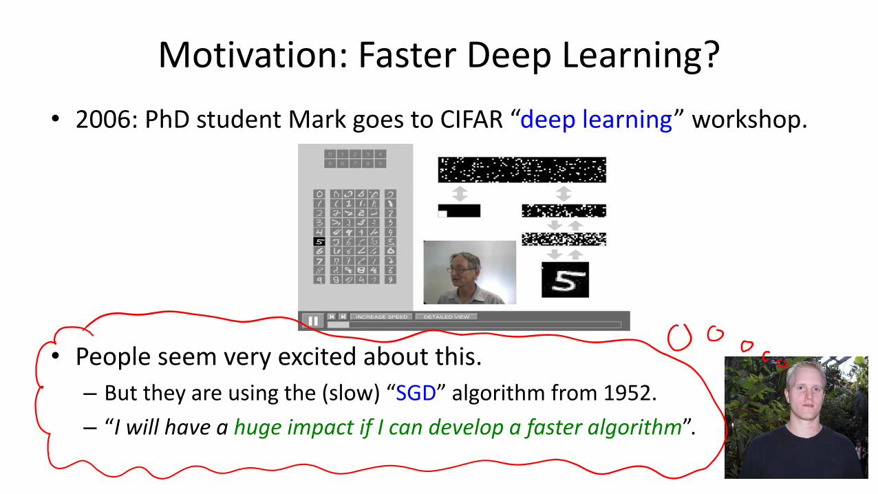
• 2006: PhD student Mark goes to CIFAR “deep learning” workshop.

• People seem very excited about this.

– But they are using the (slow) “SGD” algorithm from 1952.

– “I will have a huge impact if I can develop a faster algorithm”.

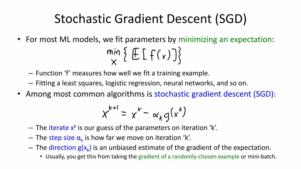
Stochastic Gradient Descent (SGD)

• For most ML models, we fit parameters by minimizing an expectation:

– Function ‘f’ measures how well we fit a training example.

– Fitting a least squares, logistic regression, neural networks, and so on.

• Among most common algorithms is stochastic gradient descent (SGD):

– The iterate xk is our guess of the parameters on iteration ‘k’.

– The step size αk is how far we move on iteration ‘k’.

– The direction g(xk) is an unbiased estimate of the gradient of the expectation.• Usually, you get this from taking the gradient of a randomly-chosen example or mini-batch.

Stochastic Gradient Descent (SGD)

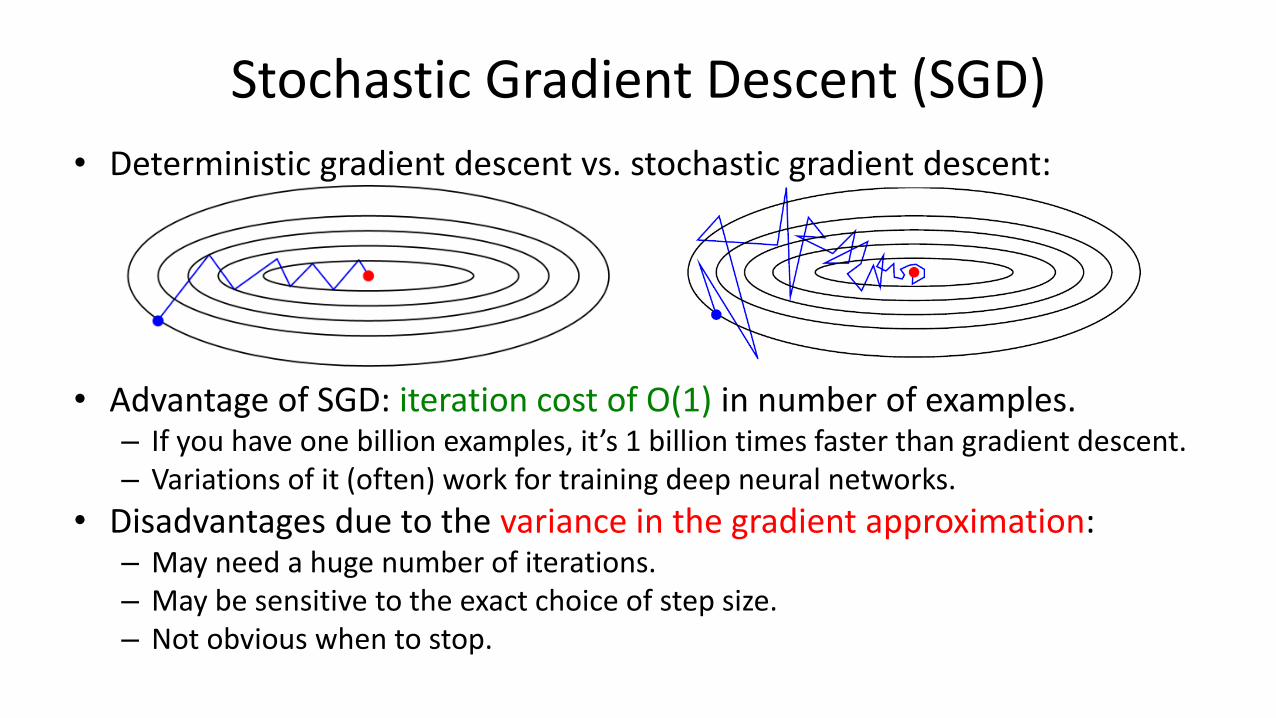
• Deterministic gradient descent vs. stochastic gradient descent:

• Advantage of SGD: iteration cost of O(1) in number of examples.– If you have one billion examples, it’s 1 billion times faster than gradient descent.– Variations of it (often) work for training deep neural networks.

• Disadvantages due to the variance in the gradient approximation:– May need a huge number of iterations.– May be sensitive to the exact choice of step size.– Not obvious when to stop.

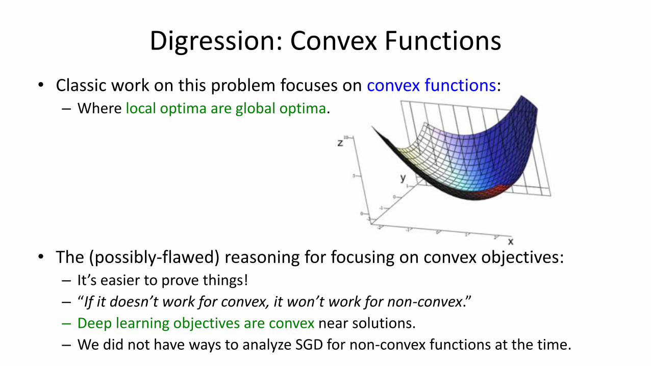
Digression: Convex Functions

• Classic work on this problem focuses on convex functions:– Where local optima are global optima.

• The (possibly-flawed) reasoning for focusing on convex objectives:– It’s easier to prove things!

– “If it doesn’t work for convex, it won’t work for non-convex.”

– Deep learning objectives are convex near solutions.

– We did not have ways to analyze SGD for non-convex functions at the time.

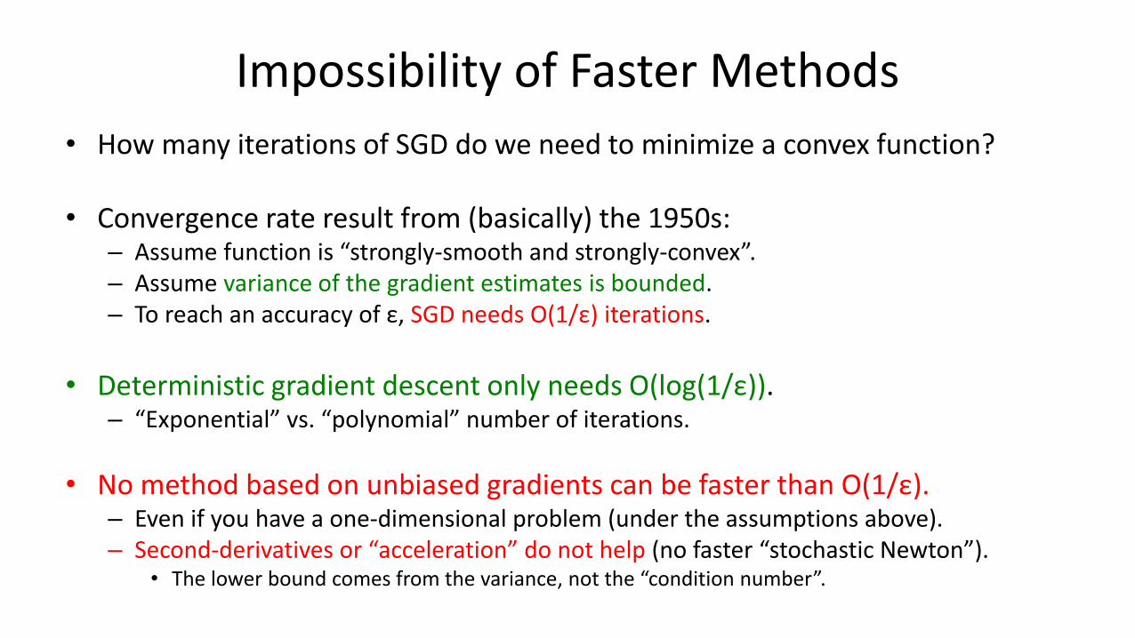
Impossibility of Faster Methods

• How many iterations of SGD do we need to minimize a convex function?

• Convergence rate result from (basically) the 1950s:– Assume function is “strongly-smooth and strongly-convex”.– Assume variance of the gradient estimates is bounded.– To reach an accuracy of ε, SGD needs O(1/ε) iterations.

• Deterministic gradient descent only needs O(log(1/ε)).– “Exponential” vs. “polynomial” number of iterations.

• No method based on unbiased gradients can be faster than O(1/ε). – Even if you have a one-dimensional problem (under the assumptions above).– Second-derivatives or “acceleration” do not help (no faster “stochastic Newton”).

• The lower bound comes from the variance, not the “condition number”.

The Assumptions

• In order to go faster than O(1/ε), we need stronger assumptions.

– Otherwise, the lower bound says it’s impossible.

• We explored two possible stronger assumptions to get O(log(1/ε)):

1. Assume you only have a finite training set.

• Usually don’t have infinite data, so design an algorithm that exploits this.

2. Cheat by finding stronger assumptions where plain SGD would go fast.

• Could explain practical success, and might suggest new methods.

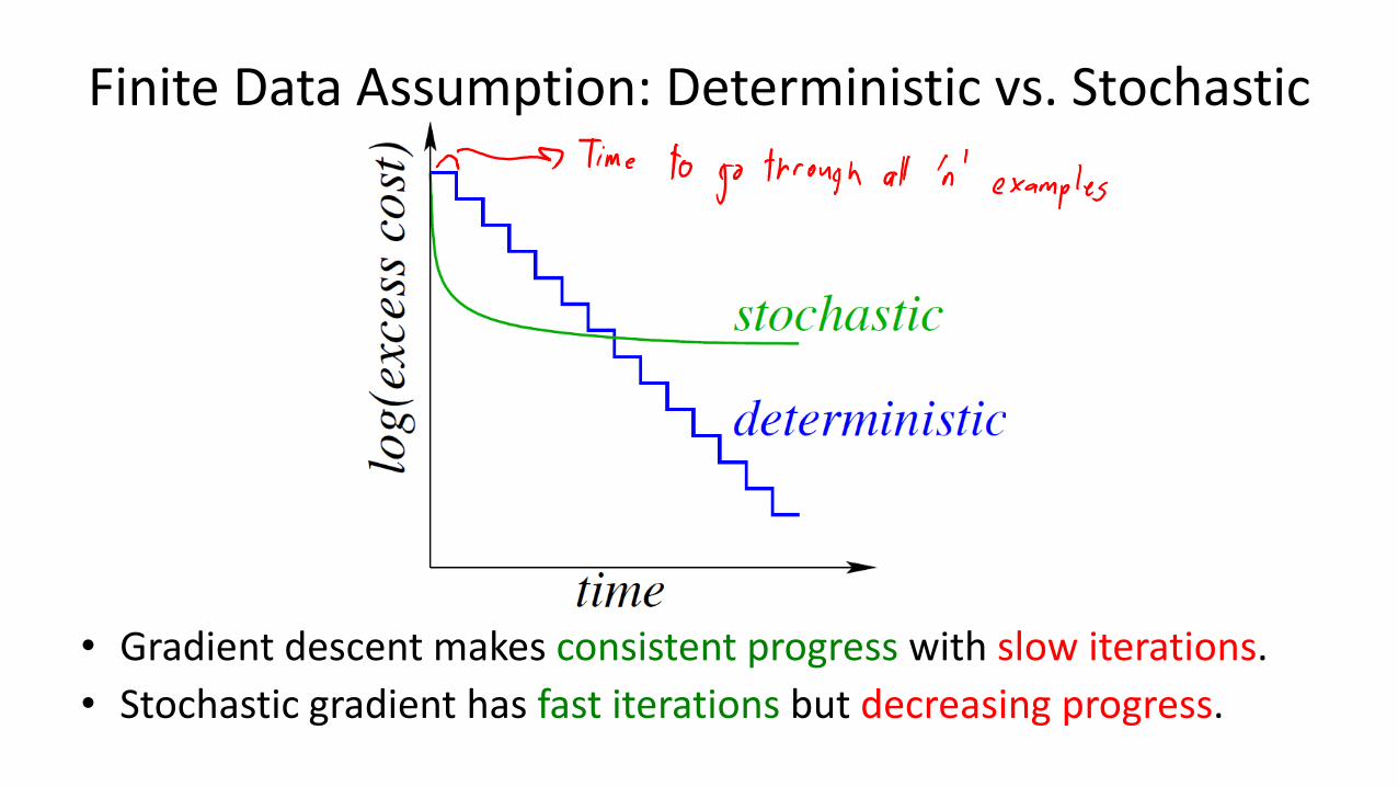
Finite Data Assumption: Deterministic vs. Stochastic

• Gradient descent makes consistent progress with slow iterations.

• Stochastic gradient has fast iterations but decreasing progress.

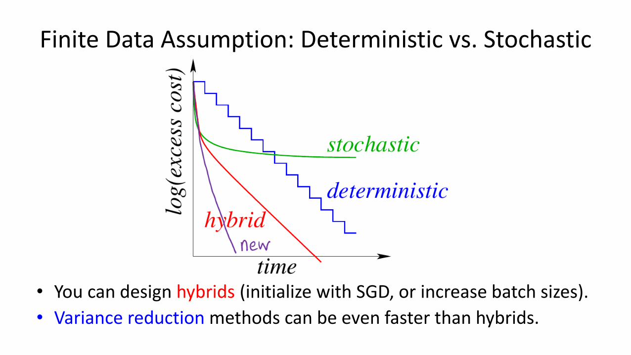
Finite Data Assumption: Deterministic vs. Stochastic

• You can design hybrids (initialize with SGD, or increase batch sizes).

• Variance reduction methods can be even faster than hybrids.

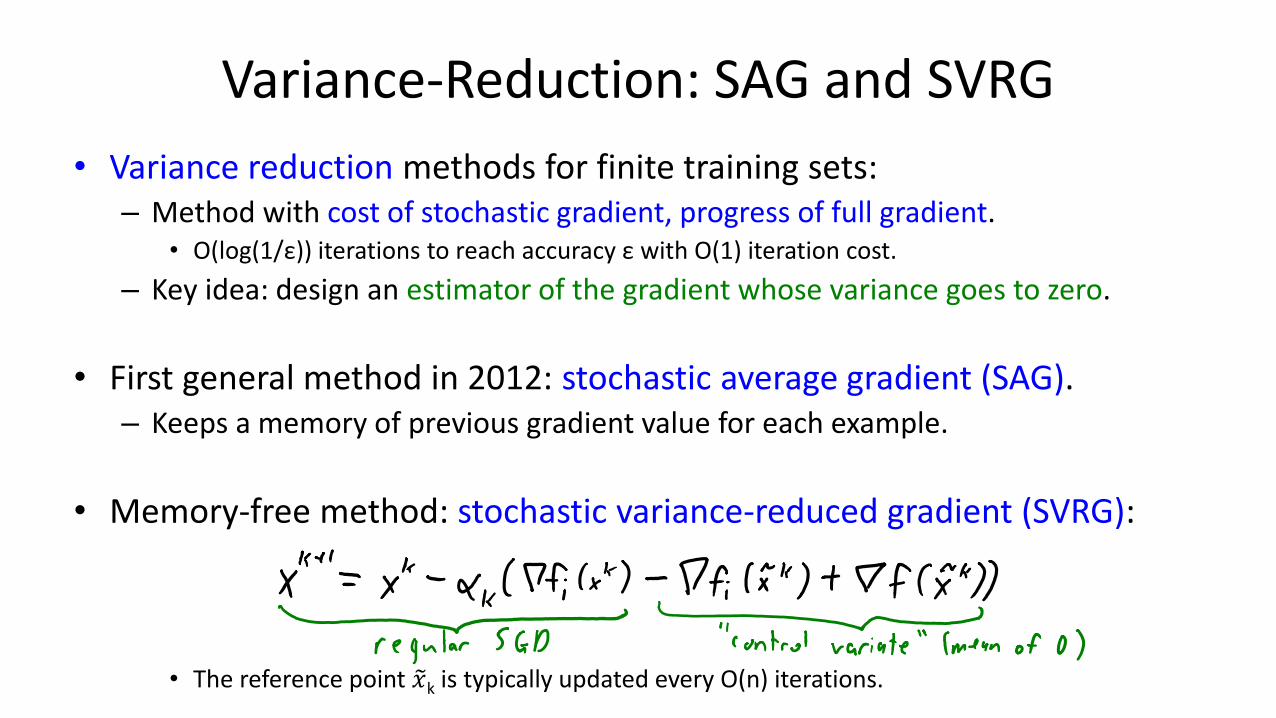
Variance-Reduction: SAG and SVRG

• Variance reduction methods for finite training sets:– Method with cost of stochastic gradient, progress of full gradient.

• O(log(1/ε)) iterations to reach accuracy ε with O(1) iteration cost.

– Key idea: design an estimator of the gradient whose variance goes to zero.

• First general method in 2012: stochastic average gradient (SAG).– Keeps a memory of previous gradient value for each example.

• Memory-free method: stochastic variance-reduced gradient (SVRG):

• The reference point 𝑥k is typically updated every O(n) iterations.

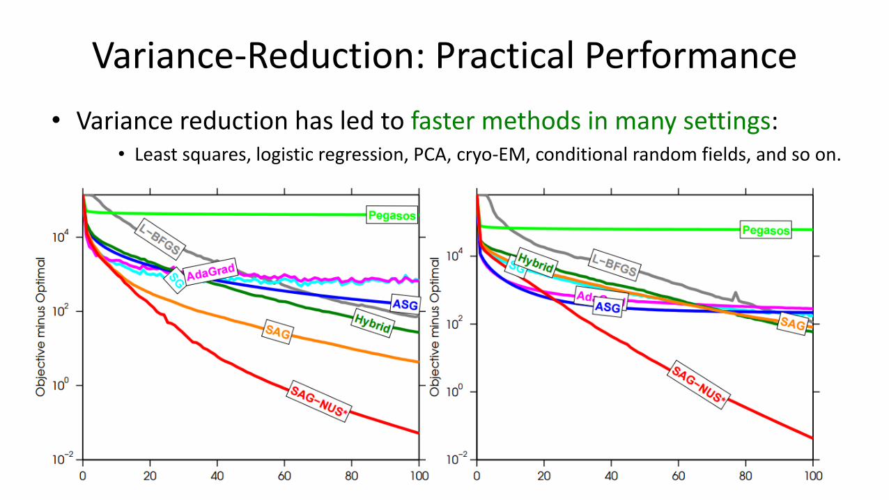
Variance-Reduction: Practical Performance

• Variance reduction has led to faster methods in many settings:• Least squares, logistic regression, PCA, cryo-EM, conditional random fields, and so on.

Variance Reduction: 8 Years Later.

• Variance reduction has been taken in a wide variety of directions:

– Memory-free SAG in some settings (like linear and graphical models).

– Variants giving faster algorithms for some non-smooth problems.

– Variants giving faster algorithms for some non-convex problems.

• Including PCA and problems satisfying the “PL inequality”.

– Momentum-like variants that achieve acceleration.

– Improved test error bounds compared to SGD.

– Parallel and distributed versions.

– SAG won 2018 “Lagrange Prize in Continuous Optimization”.

– Does not seem to help with deep learning.

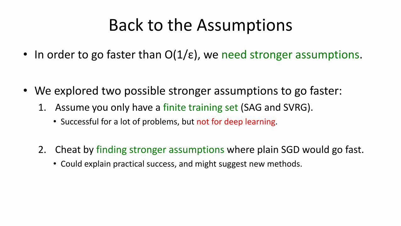
Back to the Assumptions

• In order to go faster than O(1/ε), we need stronger assumptions.

• We explored two possible stronger assumptions to go faster:

1. Assume you only have a finite training set (SAG and SVRG).

• Successful for a lot of problems, but not for deep learning.

2. Cheat by finding stronger assumptions where plain SGD would go fast.

• Could explain practical success, and might suggest new methods.

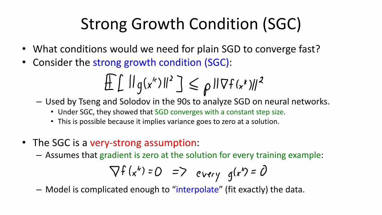
Strong Growth Condition (SGC)

• What conditions would we need for plain SGD to converge fast?• Consider the strong growth condition (SGC):

– Used by Tseng and Solodov in the 90s to analyze SGD on neural networks.• Under SGC, they showed that SGD converges with a constant step size.• This is possible because it implies variance goes to zero at a solution.

• The SGC is a very-strong assumption:– Assumes that gradient is zero at the solution for every training example:

– Model is complicated enough to “interpolate” (fit exactly) the data.

Strong Growth Condition (SGC)

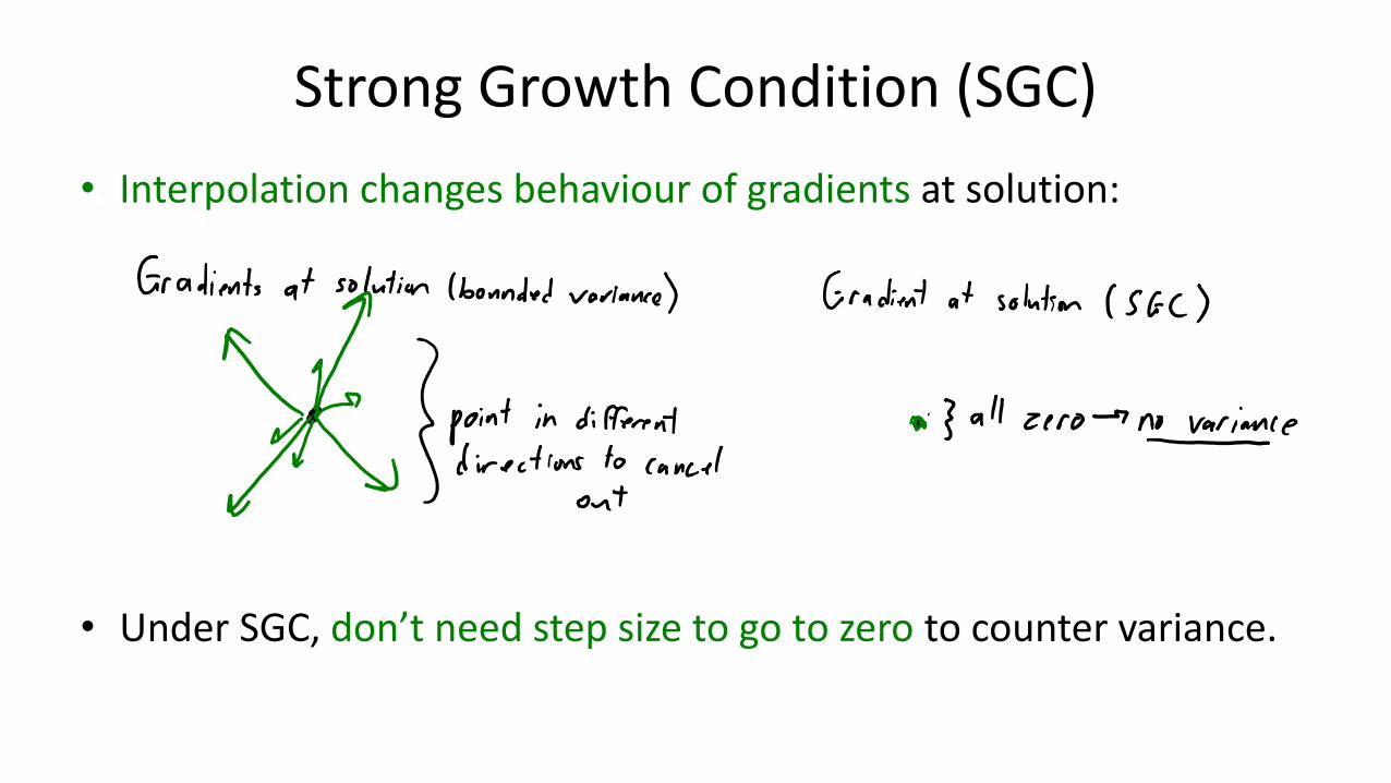
• Interpolation changes behaviour of gradients at solution:

• Under SGC, don’t need step size to go to zero to counter variance.

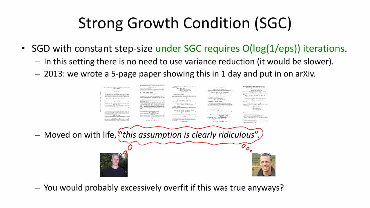
• SGD with constant step-size under SGC requires O(log(1/eps)) iterations.– In this setting there is no need to use variance reduction (it would be slower).

– 2013: we wrote a 5-page paper showing this in 1 day and put in on arXiv.

– Moved on with life, “this assumption is clearly ridiculous”.

– You would probably excessively overfit if this was true anyways?

Strong Growth Condition (SGC)

Interpolation and Deep Learning?

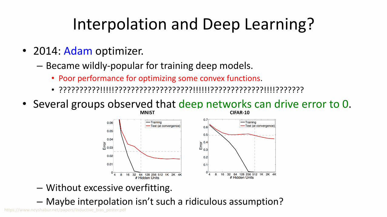
• 2014: Adam optimizer.– Became wildly-popular for training deep models.

• Poor performance for optimizing some convex functions.

• ??????????!!!!!???????????????????!!!!!!?????????????!!!!???????

• Several groups observed that deep networks can drive error to 0.

– Without excessive overfitting.

– Maybe interpolation isn’t such a ridiculous assumption?https://www.neyshabur.net/papers/inductive_bias_poster.pdf

Over-Parameterization and Interpolation

• Ma, Bassily, and Belkin [ICML, 2018]:

– Show that SGD under interpolation has linear convergence rate.

– Provided theoretical justification (and limits) for “linear scaling rule”.

– Discussed connection between interpolation and over-parameterization.

• “Over-parameterization”:

– You have so many parameters that you can drive the loss to 0.

– True for many modern deep neural networks.

– Also true for linear models with a sufficiently-expressive basis.

• You can make it true by making model more complicated (more features = fast SGD).

• Several groups explored implicit regularization of SGD (may not ridiculously ovefit).

Back to the SGC?

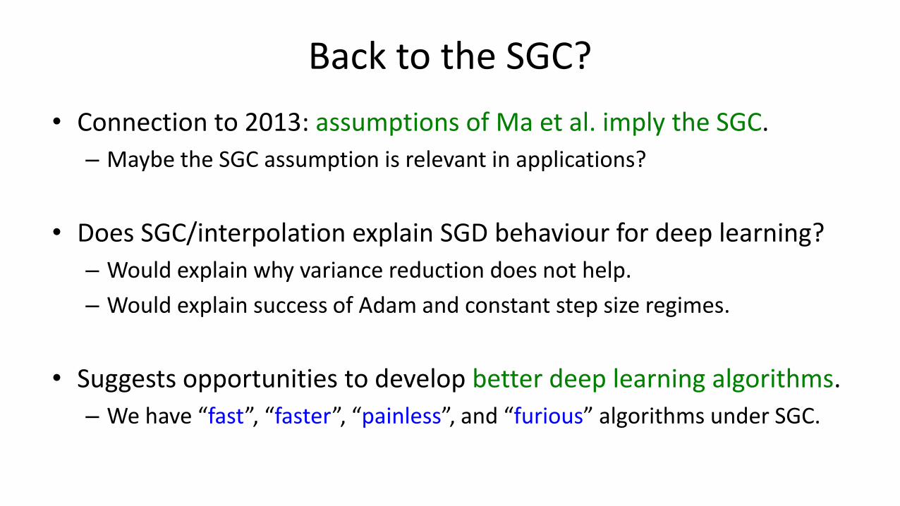
• Connection to 2013: assumptions of Ma et al. imply the SGC.

– Maybe the SGC assumption is relevant in applications?

• Does SGC/interpolation explain SGD behaviour for deep learning?

– Would explain why variance reduction does not help.

– Would explain success of Adam and constant step size regimes.

• Suggests opportunities to develop better deep learning algorithms.

– We have “fast”, “faster”, “painless”, and “furious” algorithms under SGC.

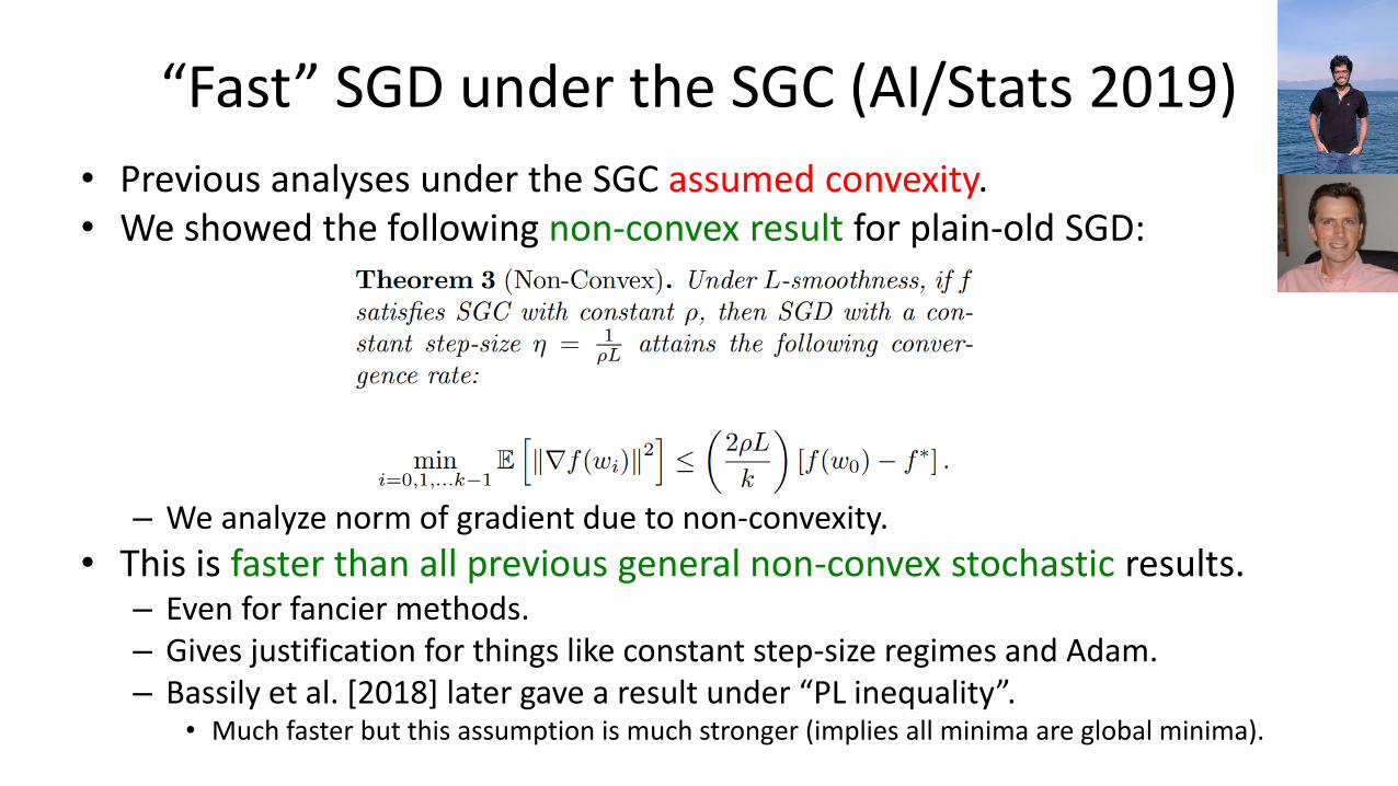
“Fast” SGD under the SGC (AI/Stats 2019)

• Previous analyses under the SGC assumed convexity.• We showed the following non-convex result for plain-old SGD:

– We analyze norm of gradient due to non-convexity.

• This is faster than all previous general non-convex stochastic results.– Even for fancier methods.– Gives justification for things like constant step-size regimes and Adam.– Bassily et al. [2018] later gave a result under “PL inequality”.

• Much faster but this assumption is much stronger (implies all minima are global minima).

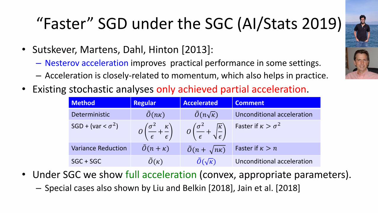
“Faster” SGD under the SGC (AI/Stats 2019)

• Sutskever, Martens, Dahl, Hinton [2013]:– Nesterov acceleration improves practical performance in some settings.

– Acceleration is closely-related to momentum, which also helps in practice.

• Existing stochastic analyses only achieved partial acceleration.

• Under SGC we show full acceleration (convex, appropriate parameters).– Special cases also shown by Liu and Belkin [2018], Jain et al. [2018]

Method Regular Accelerated Comment

Deterministic 𝑂(𝑛𝜅) 𝑂(𝑛 𝜅) Unconditional acceleration

SGD + (var < 𝜎2)𝑂

𝜎2

𝜖+

𝜅

𝜖𝑂

𝜎2

𝜖+

𝜅

𝜖

Faster if 𝜅 > 𝜎2

Variance Reduction 𝑂(𝑛 + 𝜅) 𝑂(𝑛 + 𝑛𝜅) Faster if 𝜅 > 𝑛

SGC + SGC 𝑂(𝜅) 𝑂( 𝜅) Unconditional acceleration

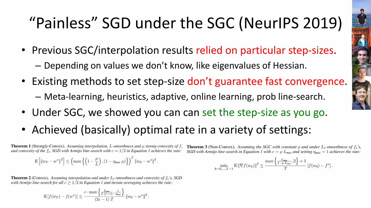
“Painless” SGD under the SGC (NeurIPS 2019)

• Previous SGC/interpolation results relied on particular step-sizes.

– Depending on values we don’t know, like eigenvalues of Hessian.

• Existing methods to set step-size don’t guarantee fast convergence.

– Meta-learning, heuristics, adaptive, online learning, prob line-search.

• Under SGC, we showed you can can set the step-size as you go.

• Achieved (basically) optimal rate in a variety of settings:

“Painless” SGD under the SGC (NeurIPS 2019)

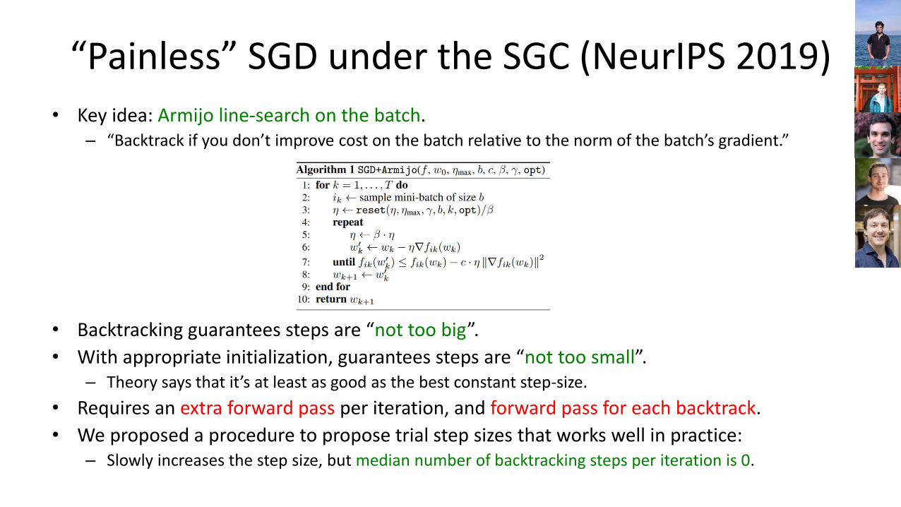
• Key idea: Armijo line-search on the batch.– “Backtrack if you don’t improve cost on the batch relative to the norm of the batch’s gradient.”

• Backtracking guarantees steps are “not too big”.

• With appropriate initialization, guarantees steps are “not too small”.– Theory says that it’s at least as good as the best constant step-size.

• Requires an extra forward pass per iteration, and forward pass for each backtrack.

• We proposed a procedure to propose trial step sizes that works well in practice:– Slowly increases the step size, but median number of backtracking steps per iteration is 0.

“Painless” SGD under the SGC (NeurIPS 2019)

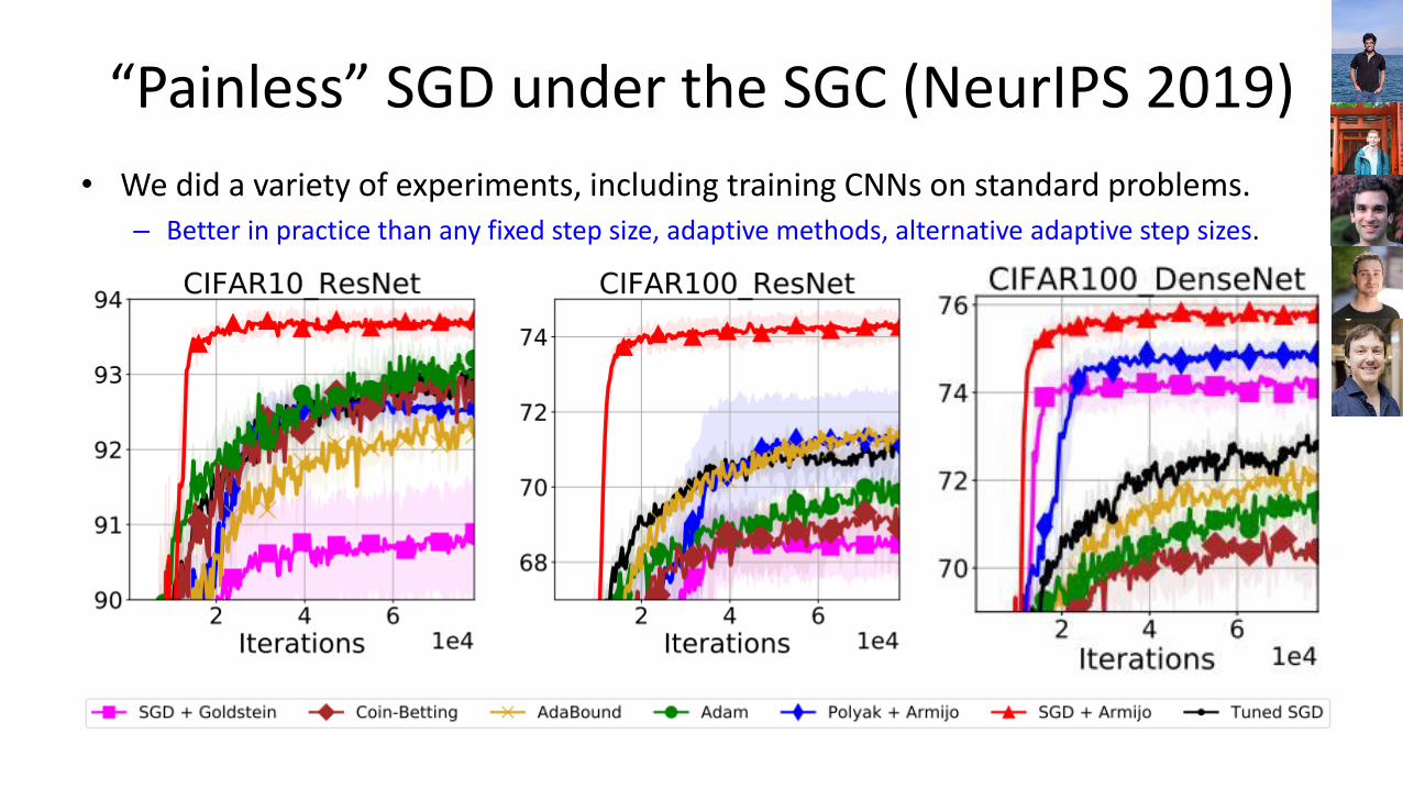
• We did a variety of experiments, including training CNNs on standard problems.– Better in practice than any fixed step size, adaptive methods, alternative adaptive step sizes.

Discussion: Sensitivity to Assumptions

• To ease some of your anxiety/skepticism:– You don’t need to run it to the point of interpolating the data, it just needs to be possible.

– Results can be modified to handle case of being “close” to interpolation.• You get an extra term depending on your step-size and how “close” you are.

– We ran synthetic experiments where we controlled the degree of over-parameterization:• If it’s over-parameterized, the stochastic line search works great.

• If it’s close to being over-parameterized, it still works really well.

• If it’s far from being over-parameterized, it catastrophically fails.

– Another group [Berrada, Zisserman, Pawan Kumar] proposed a similar method a few days later.

– We’ve compared to a wide variety of existing methods to set the step size.

• To add some anxiety/skepticism:– My students said all the neural network experiments were done with batch norm.

– They had more difficulty getting it to work for LSTMs (“first thing we tried” didn’t work here).

– Some of the line-search results have extra “sneaky” assumptions I would like to remove.

“Furious” SGD under the SGC (AI/Stats 2020)

• The reason “stochastic Newton” can’t improve rate is the variance.

• SGC gets rid of the variance, so stochastic Newton makes sense.

• Under SGC:

– Stochastic Newton gets “linear” convergence with constant batch size.

• Previous works required fininte-sum assumption or exponentially-growing batch size.

– Stochastic Newton gets “quadratic” with exponentially-growing batch.

• Previous works required faster-than-exponential growing batch size for “superlinear”.

• The paper gives a variety of other results and experiments.

– Self-concordant analysis, L-BFGS analysis, Hessian-free implementation.

Take-Home Messages

• For under-parameterized models, use variance reduction.• For over-parameterized models, don’t use variance reduction.

• New algorithms and/or analyses for over-parameterized models:– “Fast” non-convex convergence rates for plain SGD.– “Faster” SGD using acceleration.– “Painless” SGD using line-search.– “Furious” SGD using second-order information.

• Try out the line-search, we want to make it a black box code.– It will helpful to know cases where it does and doesn’t work.

• Variance-reduction might still be relevant for deep learning:– Reducing Noise in GAN Training with Variance Reduced Extragradient. T. Chavdarova, G.

Gidel, F. Fleuret, S. Lacoste-Julien [NeurIPS, 2019].