FastPD: MRF inference via the primal-dual schema

Nikos Komodakis

Tutorial at ICCV (Barcelona, Spain, November 2011)

The primal-dual schema Say we seek an optimal solution x* to the following

integer program (this is our primal problem):

(NP-hard problem)

To find an approximate solution, we first relax the integrality constraints to get a primal & a dual linear program:

primal LP: dual LP:

The primal-dual schema Goal: find integral-primal solution x, feasible dual

solution y such that their primal-dual costs are “close enough”, e.g.,

Tb y Tc x

primal cost of solution x

primal cost of solution x

dual cost of solution y

dual cost of solution y

*Tc x

cost of optimal integral solution x*

cost of optimal integral solution x*

*fT

T

c x

b y

**f

T

T

c x

c x

Then x is an f*-approximation to optimal solution x*

Then x is an f*-approximation to optimal solution x*

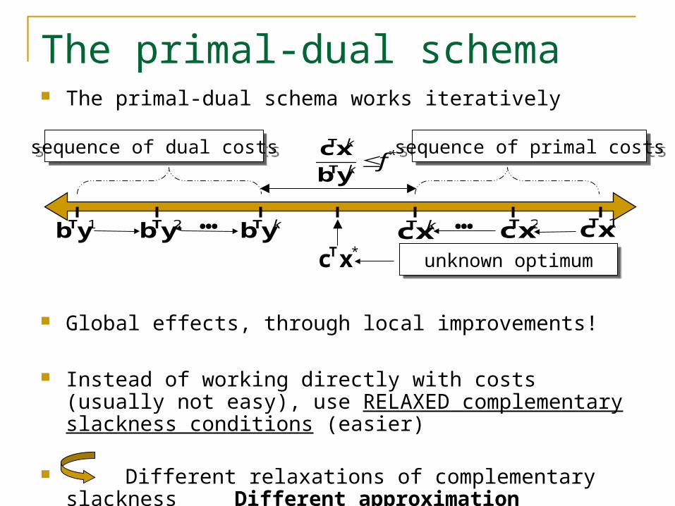
The primal-dual schema

1Tb y 1Tc x

sequence of dual costssequence of dual costs sequence of primal costssequence of primal costs

2Tb y … kTb y*Tc x unknown optimumunknown optimum

2Tc x…kTc x

k*

kf

T

T

c x

b y

The primal-dual schema works iteratively

Global effects, through local improvements!

Instead of working directly with costs (usually not easy), use RELAXED complementary slackness conditions (easier)

Different relaxations of complementary slackness Different approximation algorithms!!!

(only one label assigned per vertex)

enforce consistency between variables xp,a, xq,b and variable xpq,ab

FastPD: primal-dual schema for MRFs[Komodakis et al. 05, 07]

Binaryvariables

xp,a=1 label a is assigned to node p

xpq,ab=1 labels a, b are assigned to nodes p, q

xp,a=1 label a is assigned to node p

xpq,ab=1 labels a, b are assigned to nodes p, q

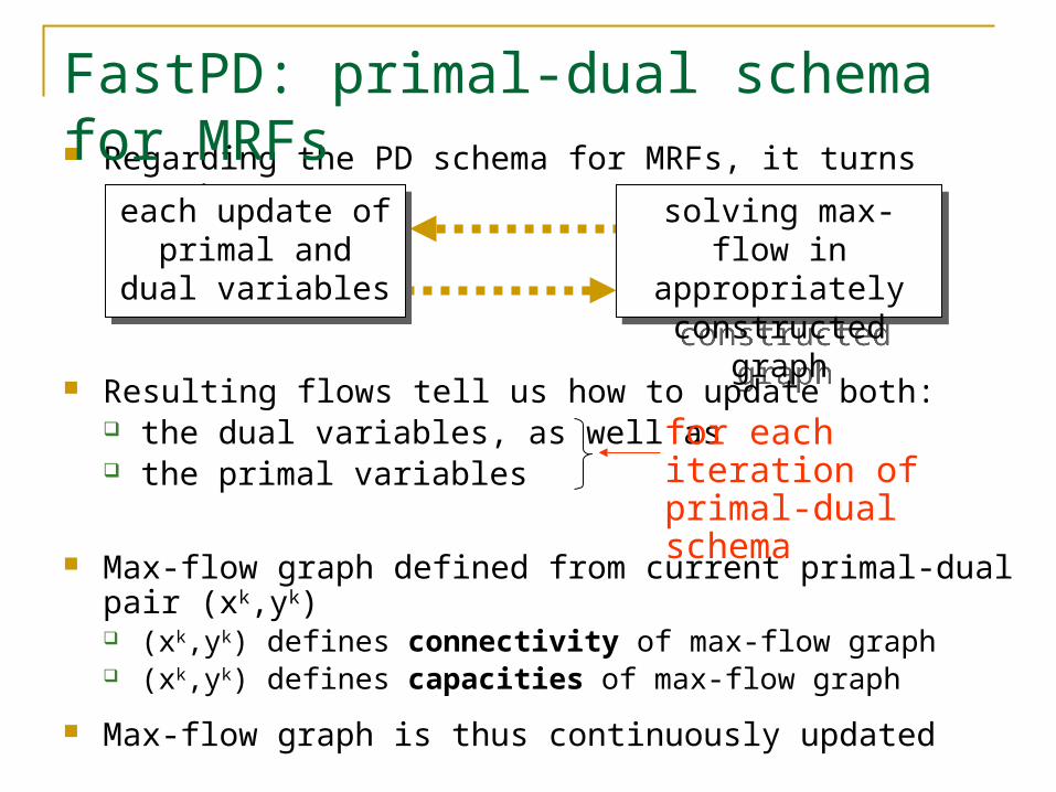
Regarding the PD schema for MRFs, it turns out that:

each update of primal and dual

variables

each update of primal and dual

variables

solving max-flow in appropriately

constructed graph

solving max-flow in appropriately

constructed graph

Max-flow graph defined from current primal-dual pair (xk,yk) (xk,yk) defines connectivity of max-flow graph (xk,yk) defines capacities of max-flow graph

Max-flow graph is thus continuously updated

Resulting flows tell us how to update both: the dual variables, as well as the primal variables

for each iteration of primal-dual schema

FastPD: primal-dual schema for MRFs

Very general framework. Different PD-algorithms by RELAXING complementary slackness conditions differently.

Theorem: All derived PD-algorithms shown to satisfy certain relaxed complementary slackness conditions

Worst-case optimality properties are thus guaranteed

E.g., simply by using a particular relaxation of complementary slackness conditions (and assuming Vpq(·,·) is a metric) THEN resulting algorithm shown equivalent to a-expansion![Boykov,Veksler,Zabih] PD-algorithms for non-metric potentials Vpq(·,·) as well

FastPD: primal-dual schema for MRFs

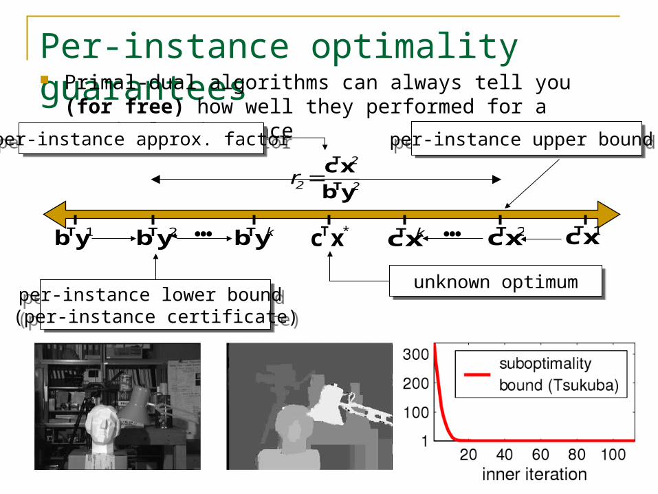
Per-instance optimality guarantees Primal-dual algorithms can always tell you (for free)

how well they performed for a particular instance

2Tb y *Tc x

unknown optimumunknown optimum

2Tc x1Tb y 1Tc x… kTb y …kTc x

T

T

c x

b y

2

2 2r

per-instance approx. factorper-instance approx. factor

per-instance lower bound (per-instance certificate)

per-instance lower bound (per-instance certificate)

per-instance upper bound per-instance upper bound

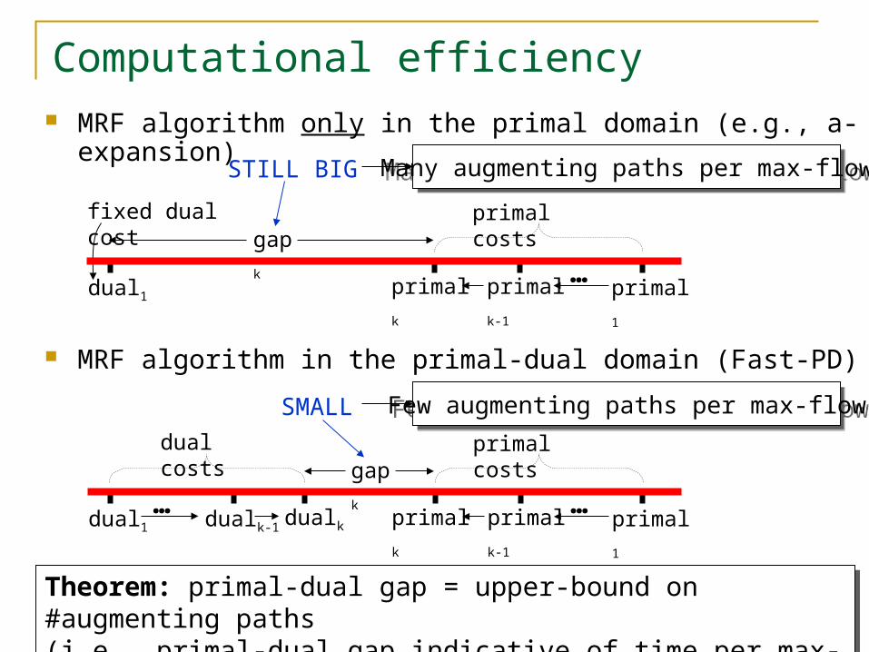
Computational efficiency MRF algorithm only in the primal domain (e.g., a-

expansion)

primalk primalk-

1

primal1…

primal costs

dual1

fixed dual costgapk

STILL BIG Many augmenting paths per max-flowMany augmenting paths per max-flow

Theorem: primal-dual gap = upper-bound on #augmenting paths(i.e., primal-dual gap indicative of time per max-flow)

Theorem: primal-dual gap = upper-bound on #augmenting paths(i.e., primal-dual gap indicative of time per max-flow)

dualkdual1 dualk-1

…

dual costs gap

kprimalk primalk-

1

primal1…

primal costs

SMALL Few augmenting paths per max-flowFew augmenting paths per max-flow

MRF algorithm in the primal-dual domain (Fast-PD)

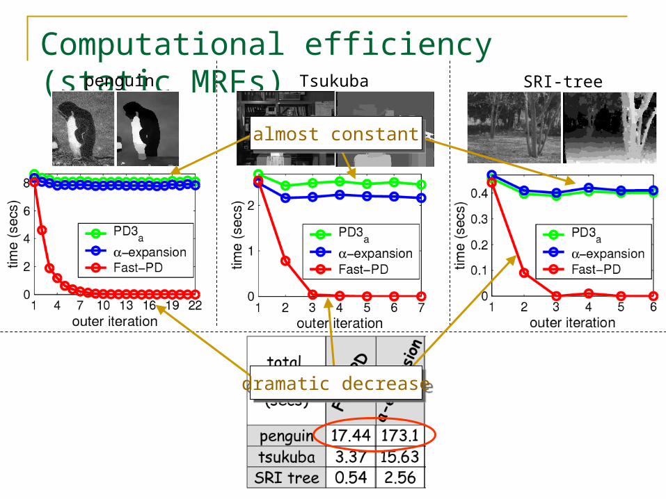
Computational efficiency (static MRFs)penguin Tsukuba SRI-tree

almost constantalmost constant

dramatic decreasedramatic decrease

primal-dual framework

primal-dual framework

Handles wide class of MRFsHandles wide class of MRFs

Approximatelyoptimal solutions

Approximatelyoptimal solutions

Theoretical guarantees AND tight certificates

per instance

Theoretical guarantees AND tight certificates

per instance

Significant speed-up

for static MRFs

Significant speed-up

for static MRFs

Significant speed-up

for dynamic MRFs

Significant speed-up

for dynamic MRFs

- New theorems- New insights into

existing techniques- New view on MRFs

- New theorems- New insights into

existing techniques- New view on MRFs

Demo session with FastPD

Demo session with FastPD

• FastPD optimization library– C++ code

(available from http://www.csd.uoc.gr/~komod/FastPD)

– Matlab wrapper

Demo session with FastPD

• In the demo we will assume an energy of the form:

,

( ) ,i i ij i ji i j

V x w D x x

Calling FastPD from C++

Step 1: Construct an MRF optimizer object

CV_Fast_PD pd( numpoints, numlabels, unary, numedges, edges, dist, max_iters, edge_weights );

Calling FastPD from C++

Step 2: do the optimization

pd.run();

Calling FastPD from C++

Step 3: get the results

for( int i = 0; i < numpoints; i++ ) {

printf( "Node %d is assigned label %d\n", i, pd._pinfo[i].label );

}

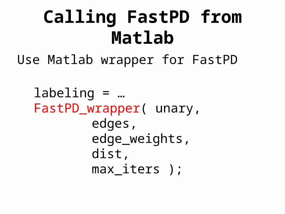
Calling FastPD from Matlab

Use Matlab wrapper for FastPD

labeling = …FastPD_wrapper( unary,

edges, edge_weights, dist, max_iters );

Run FastPD demo