Fat-tailed models for risk estimation

by Stoyan V. Stoyanov, Svetlozar T. Rachev, Boryana Racheva-Iotova, Frank J. Fabozzi

No. 30 | MAY 2011

WORKING PAPER SERIES IN ECONOMICS

KIT – University of the State of Baden-Wuerttemberg andNational Laboratory of the Helmholtz Association econpapers.wiwi.kit.edu

Impressum

Karlsruher Institut für Technologie (KIT)

Fakultät für Wirtschaftswissenschaften

Institut für Wirtschaftspolitik und Wirtschaftsforschung (IWW)

Institut für Wirtschaftstheorie und Statistik (ETS)

Schlossbezirk 12

76131 Karlsruhe

KIT – Universität des Landes Baden-Württemberg und

nationales Forschungszentrum in der Helmholtz-Gemeinschaft

Working Paper Series in Economics

No. 30, May 2011

ISSN 2190-9806

econpapers.wiwi.kit.edu

Fat-tailed models for risk estimation

Stoyan V. StoyanovEDHEC Business School

EDHEC Risk Institute–Asia

Svetlozar T. Rachev∗

Stony Brook University, USA

Karlsruhe Institute of Technology, Germany, and

FinAnalytica USA

Boryana Racheva-IotovaFinAnalytica USA

Frank J. FabozziYale School of Management

Abstract

In the post-crisis era, financial institutions seem to be more awareof the risks posed by extreme events. Even though there are attemptsto adapt methodologies drawing from the vast academic literature onthe topic, there is also skepticism that fat-tailed models are needed. Inthis paper, we address the common criticism and discuss three popularmethods for extreme risk modeling based on full distribution modelingand and extreme value theory.

∗Dr Rachev is Frey Family Foundation Chair-Professor at Department of Applied Math-ematics & Statistics, Stony Brook University. He gratefully acknowledges research supportby grants from Division of Mathematical, Life and Physical Sciences, College of Letters andScience, University of California, Santa Barbara, the Deutschen Forschungsgemeinschaftand the Deutscher Akademischer Austausch Dienst.

1

This is the submitted version of the following article: Fat-tailed Mod-els for Risk Estimation, Stoyanov, S. V., Rachev, S., Racheva-Iotova, B.,Fabozzi, F. J., Journal of Portfolio Management, 37/2, Copyright c©2011,Institutional Investor, Inc., which has been published in final form at: http:

//www.iijournals.com/doi/abs/10.3905/jpm.2011.37.2.107

1 Introduction

The extreme losses which occurred in the financial crisis of 2008 raised thequestion of whether existing models and practices, largely based on the Gaus-sian distribution represent an adequate and reliable framework for risk mea-surement and management. Following the financial crisis, different ideasfor methodology improvements have been proffered in white papers such asSheikh and Qiao (2009) and Dubikovsky et al. (2010), drawing from theexisting literature on modeling of extreme events.

Empirical studies on the properties of asset return distributions date backto the pioneering work of Mandelbrot (1963) and Fama (1963, 1965) who re-jected the assumption of normality and suggested the class of stable Paretiandistributions as an extension to the Gaussian hypothesis. Their work led tothe consolidation of the stable Paretian hypothesis which underwent em-pirical scrutiny in the 1970s and 1980s. It was reported that even thoughstock returns exhibit tails thicker than those of the Gaussian distribution,there are a few inconsistencies between observed financial return distribu-tions and those predicted by the stable Paretian distribution. The empiricalinconsistencies are related mainly to a failure of the temporal aggregationproperty, that is, tail thickness does not change with return frequency, andthe infinite-variance property of stable laws.

Even though some of the statistical techniques used to derive these con-clusions are disputed and the class of stable laws has been suggested as aviable theoretical framework,1 alternative classes of distributions were sug-gested. Examples include the Student’s t distribution considered by Blat-tberg and Gonedes (1974), the more general class of hyperbolic distributionsconsidered by Eberlein and Keller (1995), and finite mixture of normals con-sidered by Kon (1984). Generalizing the notion of stability to other proba-bilistic schemes, Mittnik and Rachev (1993) considered geo-stable, Weibull,and other distributions. More recently, tempered stable distributions have

1See Rachev and Mittnik (2000) and the references therein.

2

been suggested as a model for asset returns because they retain some of theattractive theoretical properties of stable Paretian distributions but have afinite variance and can explain the temporal aggregation property.2

Clearly, there is no fundamental theory that can suggest a distributionalmodel for financial returns and the problem remains largely a statistical one.Nevertheless, the extensive body of empirical research carried out since the1950s leads to the following stylized facts:

(1) clustering of volatility – large price changes tend to be followed by largeprice changes and small price changes tend to be followed by small pricechanges.

(2) autoregressive behavior – price changes depend on price changes in thepast, e.g. positive price changes tend to be followed by positive pricechanges.

(3) skewness – there is an asymmetry in the upside and downside potentialof price changes.

(4) fat tails – the probability of extreme profits or losses is much largerthan predicted by the normal distribution. Tail thickness varies fromasset to asset.

(5) temporal behavior of tail thickness – the probability of extreme profitsor losses can change through time; it is smaller in regular markets andmuch larger in turbulent markets.

(6) tail thickness varies across frequencies – high-frequency data tends tobe more fat-tailed than lower-frequency data.

A methodology for risk measurement can be based on any statistically ac-ceptable time-series model capable of capturing these stylized facts and anappropriate risk measure.

Apart from the full distribution modeling, there exists another methodfor modeling extreme events. It is based on the extreme value theory (EVT)developed to model extreme events in nature, such as extreme winds, tem-peratures, and river levels, and provides a model only for the tails for the

2See Kim et al. (2008) and Samorodnitsky and Grabchak (2010).

3

distribution. Embrechts et al. (1997) provide applications in the field ofinsurance and finance.

In the post-crisis era, while on the surface there seems to be universalagreement that financial assets are indeed fat-tailed and that investmentmanagers must take extreme events into account as part of their everydayrisk management processes, the attitude in the academic circles is not as uni-form. There are constructive efforts to identify factors explaining tail eventswhich can, potentially, be hedged (see Bhansali (2008)), or verify whetherthe observed dynamics in correlations during market crashes are not artifactsof the implicit assumption of normality (see Campbell et al. (2008)). Yet,in stark contrast, there are papers such as Esch (2010) suggesting fat-tailedmodels should be ignored in favor of Gaussian-based models on the groundsof parsimony. While from a statistical viewpoint simpler models explainingall stylized facts of the data are preferred to more complex models, represen-tativity should not be sacrificed for simplicity. In other words, models shouldbe as simple as possible but not any simpler.

The paper is organized in the following way. Section 2 discusses whethernon-Gaussian models in general are really needed. Sections 3 and 4 focus onthe two common techniques for modeling extreme losses. Finally, Section 5discusses general techniques for model selection.

2 Are non-Gaussian models needed?

Since fat-tailed models challenge well-established classical theories, there hasbeen a natural resistance towards them both in academia and in the practiceof finance. The resistance is usually not rooted in doubts whether fat-tailsexist in the real world; first, empirical research has firmly established thisfact and, second, the fresh memories of the recent financial crisis are foodfor thought for those in denial. Rather, it is based on pragmatic reasoningwhich can be summarized in the following two statements: (i) the classicalmodels are preferred because any attempt to employ a non-Gaussian modelnecessarily results in huge estimation errors which introduce additional un-certainty and outweigh the benefits and (ii) the observed fat tails can beexplained through Gaussian-based classical models. In this section, we con-sider in detail each of these statements.

4

2.1 Estimation errors and non-Gaussian models

The discussion of estimation errors and non-Gaussian models has two aspectsand we draw a clear distinction between them. The first aspect concerns ap-plication of higher-order moments in order to account for a potential skewnessand excess kurtosis which are two geometric characteristics of the return dis-tribution representing deviations from normality. The usual approach is totake advantage of the classical statistical measures of skewness and kurtosisand to use them directly in an extension of the classical mean-variance anal-ysis for portfolio construction (see Martellini and Ziemann (2010)) or to usethem for the purpose of value-at-risk (VaR) estimation through a moment-based approximation known as the Cornish-Fisher expansion. It is importantto note that this approach is not related to a fat-tailed distribution and isnon-parametric in nature. Loosely speaking, the goal is to describe devia-tions from normality in geometric terms using two descriptive statistics inaddition to mean and volatility.

The criticism of this approach summarized by Esch (2010) is basicallycentered on the fact that the classical estimators of skewness and kurtosisexhibit significant variability to the input sample and, therefore, reliable esti-mation is difficult. Martellini and Ziemann (2010) extend the discussion intoa multivariate setting arguing that the curse of dimensionality exacerbatesfurther the estimation problem.

The instability of the classical estimators is a well-known problem in thefield of statistics and alternative robustified estimators have been developed.As noted by Martellini and Ziemann (2010), one possible approach in an assetallocation context is to introduce a structure in the covariance, co-skewnessand co-kurtosis of asset returns by means of a factor model which reducessampling error at the cost of specification error. Also, shrinkage estimatorscan be considered as they provide an optimal trade-off between sampling andspecification error. Finally, as far as the one-dimensional problem of skew-ness and kurtosis estimation of a single asset is concerned, there are robustquantile-based estimators which are much more reliable than the classicalestimators.

Dismissing the non-parametric approach on the basis of the properties ofclassical estimators for skewness and kurtosis is a hurried decision. Martelliniand Ziemann (2010) conclude that there can be a significant value added inasset allocation decisions if the estimation problem is handled properly.

The extension of the mean-variance analysis with skewness and kurto-

5

sis is, essentially, based on a higher-order Taylor series approximation ofexpected utility and is well-motivated by theory. However, employing thenon-parametric method for downside risk estimation leads to other difficul-ties. From a conceptual viewpoint, while skewness and kurtosis do describedeviations from the Gaussian distribution in geometric terms, they do notfocus on the downside of the return distribution. The described deviationsfrom normality more or less concern the central part of the distribution andthere are no reasons to believe that a skewed distribution with an excess kur-tosis will better describe extreme losses. For any distribution, skewness andkurtosis represent two numbers and it is impossible to describe the richnessof the possible shapes of the tail behavior only in terms these two numbers.

As a result, for the purposes of risk estimation it is better to rely on othertechniques especially when quantiles deep in the tail are involved. Thesetechniques involve assuming a fat-tailed model that can describe the tail ofthe empirical distribution and bring up the second aspect of the discussionon estimation errors and non-Gaussian models. Fat-tailed models have pa-rameters that are related to their tail behavior and skewness in additionto the mean and scale3 parameters meaning the number of parameters ofa fat-tailed distribution exceeds the number of parameters of the normaldistribution which results in additional complexity. The common argumentsummarized by Esch (2010) is that the notion of parsimony dictates simplermodels are better because complexity may turn out to be redundant whichis not easily detectable in-sample.

This is a very general philosophical argument which is counter-productiveif used without further analysis. First, additional complexity may be neededin order to explain observed facts and this holds not only for finance but forthe realm of science in general. If skewness and fat-tails are observed in thereal world, it is only natural to choose a family of distributions that can takeinto account the empirical facts at the cost of introducing two additionalparameters. Model selection techniques can be employed to assess whetherthe improvement of the extended model is statistically significant.

Second, it is incorrect to think that fat-tailed models are alternatives tothe Gaussian model. In fact, most classes of fat-tailed distributions containthe Gaussian distribution as a special case. In this sense, they truly extendthe framework and if the data is Gaussian, then the model would recognizethis fact. There are statistical techniques for hypothesis testing that can

3Volatility describes the “scale” of the normal distribution.

6

verify if the fitted parameters of the fat-tailed model are significantly differentfrom the parameter values identifying the normal distribution. The labels“non-Gaussian” and “fat-tailed” as opposed to “Gaussian” and “non-fat-tailed” are supposed to reflect the underlying properties and not to implythat these models cannot co-exist in a more general framework.

From this perspective, the Gaussian model itself represents a significantrestriction that can lead to overly optimistic risk numbers in times of crashesand realistic numbers in ordinary market conditions. Thus, as far as themodeling philosophy is concerned, it is better to start with a more generalmodel and restrict it only if the impact of the “noise” coming from theadditional complexity outweighs the benefits.

2.2 Explanations of fat-tails through Gaussian-basedmodels

The main argument in this section is related to the last argument of the pre-vious section – in the light of a non-explained empirical fact, it is preferableto try to describe it first with the available tools before increasing the modelcomplexity.

There are two main approaches to explain fat-tails through Gaussianbased models. First, fat-tails appear because the volatility of asset returns isdynamic. Therefore, looking at the unconditional distribution as describedby histogram plots or kernel density plots we can see heavy tails but theyare mostly due to the time varying volatility. Second, fat-tails appear be-cause asset returns depend in a non-linear fashion on other factors which aredistributed according to a Gaussian law.

Empirical research has firmly established the fact that volatility clusteringis a stylized fact of asset returns.4 Different econometric models have beensuggested to explain the time varying volatility and the most widely used onesare the GARCH-type models. These econometric models can be regarded asfilters that transform the empirical data by explaining certain phenomena andproduce new data, also known as residual, which is more homogeneous. Asa consequence, it is possible to run a statistical test on the residual to verifyif explaining the volatility clustering effect leads to a Gaussian distribution.Empirical research has shown even though the residual appears to be less

4For an empirical research, see for example Akgiray (1989).

7

Exhibit 1: The degrees of freedom parameter of the residuals of a time-seriesmodel fitted on the returns of the constituents of S&P500.

fat-tailed than the original data, it is not Gaussian.5

We illustrate this behavior in an empirical calculation which includes thestocks in the S&P500 universe during the 3-year period from January 1, 2007to November 1, 2010. We fitted a time series model6 to clean the clusteringof volatility effect assuming the classical Student’s t model on the residual.The degrees of freedom (DOF) parameter, which governs the tail behavior,is shown on Figure 1. The smaller the value is, the heavier the tails are. IfDOF has a value of about 30 and above, it can be argued that the Student’st distribution is close to the normal distribution.

We calculated that 27% of all stocks have a DOF above 7 and 13% havea DOF below 4 indicating a diverse tail behavior. These results agree witha similar calculation for the same universe done for a different time period,see Rachev et al. (2010). Figure 1 demonstrates that the time variationsin the volatility cannot explain the fat-tailes observed in the unconditional

5See Rachev and Mittnik (2000) and the references therein for extensive econometricstudies.

6The time series model is an ARMA(1,1)-GARCH(1,1) model.

8

distribution of stock returns. i.e. we find significant tail thickness in theresidual even though the time-series model captures the clustering of thevolatility effect.

Even though asset returns do not seem to be conditionally Gaussian,GARCH-type models are a very useful tool because they can describe thetime structure of volatility. Volatility, or more generally the scale param-eter of the distribution, is an important factor in risk estimation becauseit affects all quantiles of the return distribution including the very extremeones. Therefore, any probabilistic model for risk estimation should include aGARCH-type component.

The argument that, hypothetically, the fat-tailed behavior of asset returnscan be explained through non-linear factor models and, therefore, fat-taileddistributions are redundant is weak without any empirical justification thatsuch factor models can be reliably fitted and that the factor returns are indeednormal. This argument should be considered on a case-by-case basis and notgenerally.7 Certainly, a good non-linear factor model (or linear one for thatmatter) is a powerful tool to identify risk exposures and is instrumentalfor portfolio risk management purposes. The structure provided by such afactor model is a useful piece of information in addition to describing theshape of the portfolio return distribution. However, if it turns out that thefactor model is not reliable because of low explanatory power or if our goal isonly risk measurement, then having a good description of the (conditional)distribution of portfolio returns is sufficient.

Non-linear factor models represent a big family of diverse models. Thereare three basic types models depending on how non-linearity is introduced– (i) non-linear in the factors but linear in the parameters, (ii) non-linear inboth the factors and the parameters, and (iii) no particular functional formof the non-linearities, e.g. a kernel regression. From a parsimony standpoint,it is very easy to end up with a model that overfits the data which does notimply that non-linear factor models should be disregarded. This is a class oftechniques that can be helpful and should be used very carefully bearing inmind the potential issues.

Rachev et al. (2010) illustrate the time variations of tail thickness in thedaily returns of the DJIA index from October 1997 to October 2009. The

7The term non-linear factor model is quite general and without a specification of thenon-linear function defining the relationship is of no use. In fact, any random variablecan be represented as a non-linear factor model of factors having arbitrary pre-specifieddistributions.

9

example indicates that tail thickness may increase in times of crashes alongwith volatility implying that factors unexplained by the time-series modelmay impact downside risk. Unless these factors can be explained completelyby means of linear or non-linear factor models, it is important to adopt afat-tailed model which can provide a reasonable statistical description of thedata.

3 Full distribution modeling

Apart from the non-parametric approach based on higher-order moments,there are two approaches for modeling the tails of the return distribution.One of them is to assume fat-tailed tailed distribution and the other oneis based on EVT. The two approaches are different in nature. A fat-taileddistributional assumption represents a model for the entire distribution whileEVT-based models are designed to describe the maximum loss over a givenhorizon meaning that they are designed to describe the extreme tail only.

As mentioned before, a GARCH-type model for the scale of the return dis-tribution is of crucial importance. Therefore, the two approaches mentionedin this section have to be applied to the residual produced by applying theGARCH filter to the observed asset returns. In this section, we consider thefull distribution modeling approach represented by two Student’s t distribu-tion and tempered stable distributions.

3.1 The Student’s t distribution

First introduced in 1908, the Students t distribution is probably the mostcommonly used fat-tailed distribution as a model for asset returns. Like thenormal distribution, classical Students t densities are symmetric and have asingle peak. Unlike the normal distribution, Students t densities are morepeaked around the centre and have fatter tails.

This property is illustrated on Exhibit 2. In fact, the normal distributionis a special case when the DOF parameter approaches infinity. For practicalpurposes, however, the plot indicates a very small difference for a DOF of30. While this property makes the Student’s t distribution acceptable forasset returns modeling, the real reason behind its widespread use is its easeof application – numerical methods are easily implementable and are widelyavailable.

10

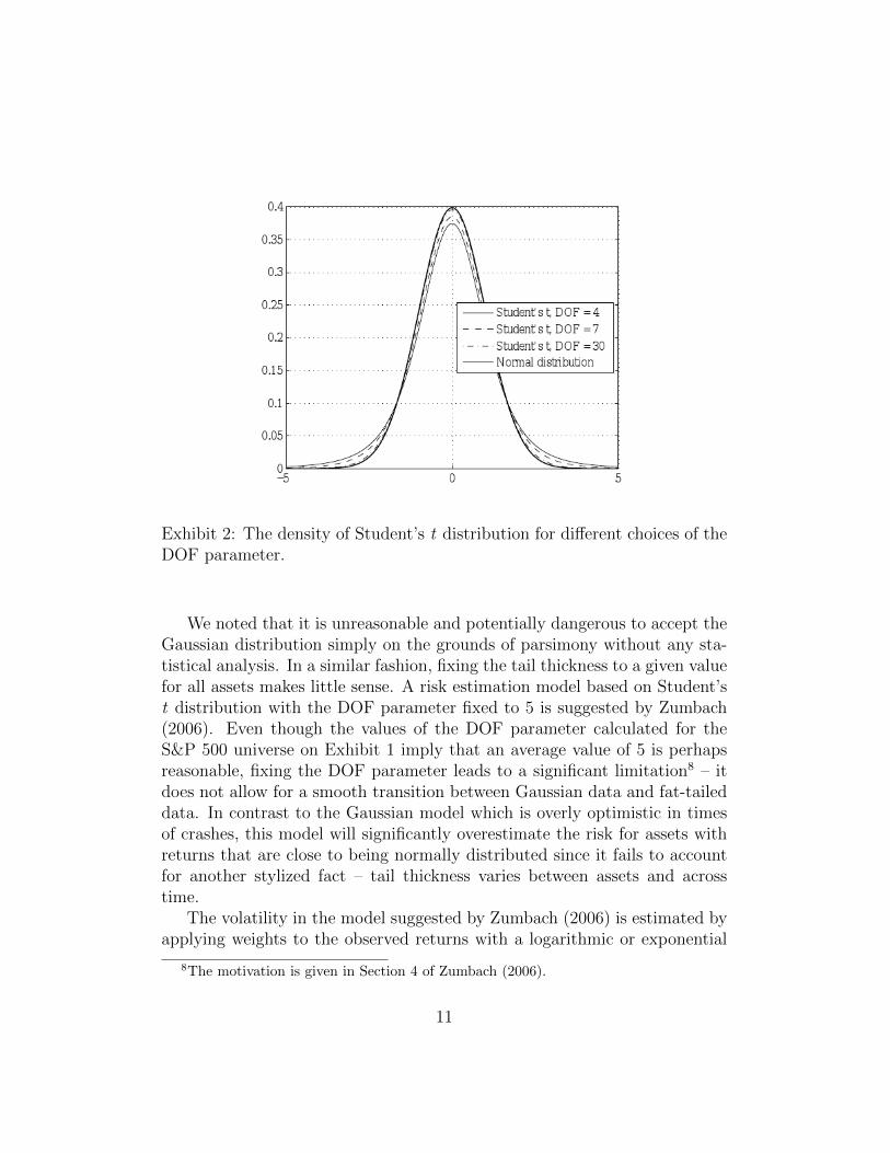
Exhibit 2: The density of Student’s t distribution for different choices of theDOF parameter.

We noted that it is unreasonable and potentially dangerous to accept theGaussian distribution simply on the grounds of parsimony without any sta-tistical analysis. In a similar fashion, fixing the tail thickness to a given valuefor all assets makes little sense. A risk estimation model based on Student’st distribution with the DOF parameter fixed to 5 is suggested by Zumbach(2006). Even though the values of the DOF parameter calculated for theS&P 500 universe on Exhibit 1 imply that an average value of 5 is perhapsreasonable, fixing the DOF parameter leads to a significant limitation8 – itdoes not allow for a smooth transition between Gaussian data and fat-taileddata. In contrast to the Gaussian model which is overly optimistic in timesof crashes, this model will significantly overestimate the risk for assets withreturns that are close to being normally distributed since it fails to accountfor another stylized fact – tail thickness varies between assets and acrosstime.

The volatility in the model suggested by Zumbach (2006) is estimated byapplying weights to the observed returns with a logarithmic or exponential

8The motivation is given in Section 4 of Zumbach (2006).

11

decay based on a predefined parameter.9 This forces the relative importanceof the observations in the past to be the same for all risk drivers and acrossall time periods. While this universal parameter makes these models simplerand easier to grasp, there is an important trade-off between simplicity andprecision: these models are less accurate and only work “on average” in auniverse of risk drivers. Even though the approach in Zumbach (2006) devi-ates from the traditional GARCH-type framework, an implementation withthe classical Student’s t distribution for the residual without the deficiency offixing the DOF parameter is available, for example, in the GARCH toolboxof MATLAB.

Finally, the classical Students t model is symmetric. In cases where thereis a significant asymmetry in the data, it will not be reflected in the riskestimate.

3.2 Tempered stable distributions

As noted in the introduction, the class of stable distributions has a specialplace among non-Gaussian full distribution models. It was suggested as amodel for asset returns because it contains the normal distribution as a spe-cial case sharing a remarkable property – only this class of distributions canapproximately describe the behavior of a stochastic system influenced bymany small, regular, and independent random factors. Since price changesare driven by many random factors, it is reasonable to assume that stabledistributions could represent a model for their approximate behavior (seeRachev and Mittnik (2000)). This was the reason the stable Paretian hy-pothesis was suggested in the 1960s.

Like the Students t distribution, stable Paretian distributions have a pa-rameter responsible for the tail behavior, which is called the tail index orindex of stability. In contrast to the DOF parameter, the index of stabilityis between zero and two. The closer it is to two, the more Gaussian like thedistribution is; smaller values of the index of stability imply a fatter tail.Unlike the Students t distribution, stable distributions allowed for skewedrepresentatives, see Exhibit 3.

The two empirical inconsistencies with the stable Paretian hypothesis isthat it implies infinite variance for asset returns and a tail behavior which

9An example is a decay parameter of the equally weighted moving average methodequal to 0.94.

12

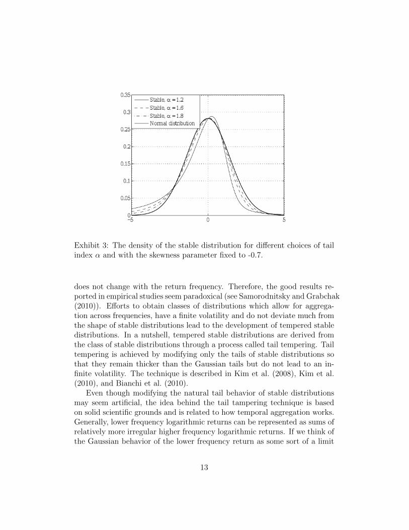
Exhibit 3: The density of the stable distribution for different choices of tailindex α and with the skewness parameter fixed to -0.7.

does not change with the return frequency. Therefore, the good results re-ported in empirical studies seem paradoxical (see Samorodnitsky and Grabchak(2010)). Efforts to obtain classes of distributions which allow for aggrega-tion across frequencies, have a finite volatility and do not deviate much fromthe shape of stable distributions lead to the development of tempered stabledistributions. In a nutshell, tempered stable distributions are derived fromthe class of stable distributions through a process called tail tempering. Tailtempering is achieved by modifying only the tails of stable distributions sothat they remain thicker than the Gaussian tails but do not lead to an in-finite volatility. The technique is described in Kim et al. (2008), Kim et al.(2010), and Bianchi et al. (2010).

Even though modifying the natural tail behavior of stable distributionsmay seem artificial, the idea behind the tail tampering technique is basedon solid scientific grounds and is related to how temporal aggregation works.Generally, lower frequency logarithmic returns can be represented as sums ofrelatively more irregular higher frequency logarithmic returns. If we think ofthe Gaussian behavior of the lower frequency return as some sort of a limit

13

behavior, then an explanation for the change in the tail behavior can be theconvergence rate to that limit. For example, monthly returns and weeklyreturns can be represented as sums of daily returns, the only difference is inthe number of summands. Intuitively, the convergence rate would be faster ifthere are more summands (higher vs lower frequencies) which are also moreregular (normal vs extreme market conditions).

The tail tempering technique arises from results in probability theorydealing with the problem of estimating the rates of convergence in limittheorems indicating that the shape of the distribution of the sum looks likea stable distribution at the center but does not have as heavy tails, seeSamorodnitsky and Grabchak (2010).

4 Extreme value theory

EVT has been applied for a long time when modeling the frequency of ex-treme events, including extreme temperatures, floods, winds and other nat-ural phenomena. From a general perspective, extreme value distributionsrepresent distributional limits for properly normalized maxima of indepen-dent random quantities with equal distributions, and therefore can be appliedin finance as well, see Embrechts et al. (1997). In contrast to the other distri-bution families mentioned in the introduction, EVT represents a model forthe tail of the distribution only. Therefore, in practice, one needs to combineEVT with a model for the remaining part of the distribution if needed.

The method behind EVT can be intuitively described in the followingway. Consider a sequence of returns at a given frequency. The maximumloss can be approximately described through a limit distribution known asthe generalized extreme value distribution (GED). Another way to modelextreme losses is to consider the exceedances over a high threshold. EVT in-dicates that asymptotically, as the high threshold increases, the exceedancescan be described by the generalized Parreto distribution (GPD).

There are many empirical studies applying EVT directly to the returntime series ignoring the clustering of volatility effect (see, for example, Marinelliet al. (2007) and Sheikh and Qiao (2009)). While at times this may be areasonable simplification for shorter time intervals, in practice the stylizedfacts mentioned in the introduction can represent significant deviations fromhypothesis that returns are independent and identically distributed (iid). Asa consequence, the stylized facts have to be modeled separately and EVT

14

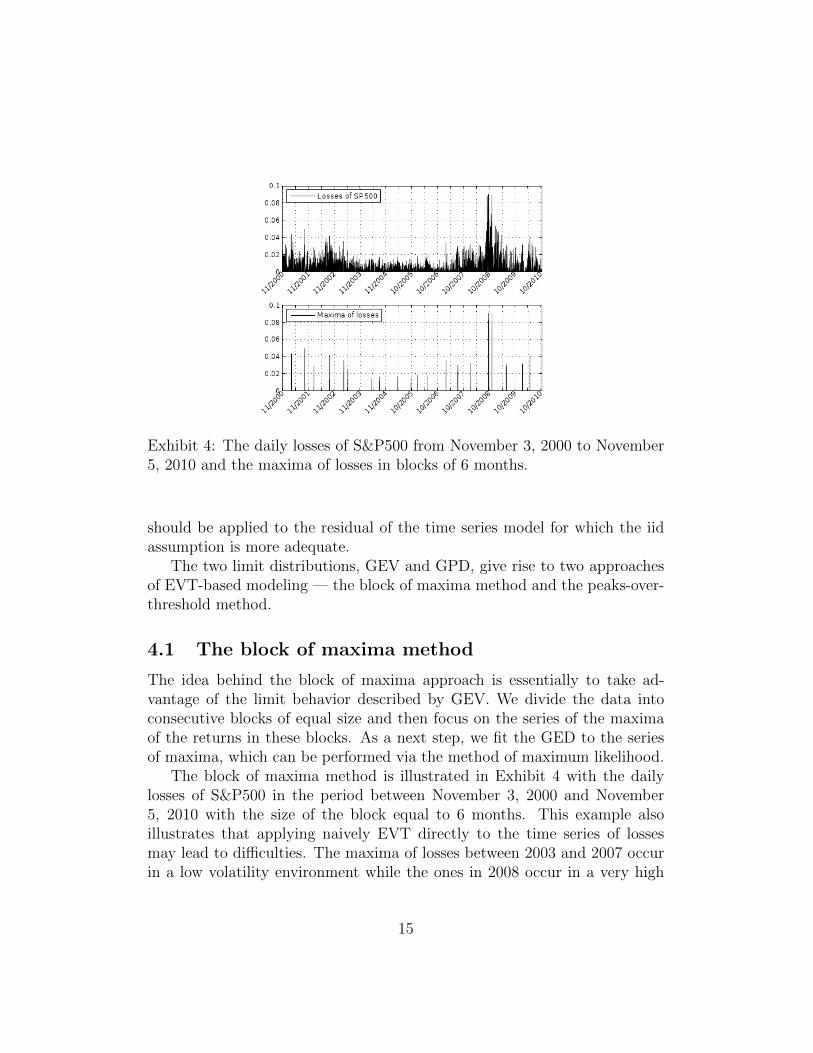
Exhibit 4: The daily losses of S&P500 from November 3, 2000 to November5, 2010 and the maxima of losses in blocks of 6 months.

should be applied to the residual of the time series model for which the iidassumption is more adequate.

The two limit distributions, GEV and GPD, give rise to two approachesof EVT-based modeling — the block of maxima method and the peaks-over-threshold method.

4.1 The block of maxima method

The idea behind the block of maxima approach is essentially to take ad-vantage of the limit behavior described by GEV. We divide the data intoconsecutive blocks of equal size and then focus on the series of the maximaof the returns in these blocks. As a next step, we fit the GED to the seriesof maxima, which can be performed via the method of maximum likelihood.

The block of maxima method is illustrated in Exhibit 4 with the dailylosses of S&P500 in the period between November 3, 2000 and November5, 2010 with the size of the block equal to 6 months. This example alsoillustrates that applying naively EVT directly to the time series of lossesmay lead to difficulties. The maxima of losses between 2003 and 2007 occurin a low volatility environment while the ones in 2008 occur in a very high

15

volatility period and, therefore, they are not generated by one and the samedistribution.

There are two practical problems with the block of maxima method: (i)the choice of the size of the blocks and (ii) the length of the time series.While for daily financial time series, the size of the block is recommendedto be three months, six months, or one year, there is no general rule ofthumb or any formal approach which could suggest a good choice. Eventhese recommendations are rather arbitrary because the size of the resultingsample of maxima can vary up to four times which naturally can exercise abig impact on the estimates.

Concerning the second problem, one needs a very large initial sample inorder to have a reliable statistical estimation. In academic examples, using20-30 years of daily returns is common, see, for example, McNeil et al. (2005).However, from a practical viewpoint, it is arguable that observations so farback in the past have any relevance to the present market conditions.

4.2 The peaks-over-threshold method

The peaks-over-threshold (POT) method arises from the limit result leadingto GPD. Like the block of maxima method, the parameters of GPD canbe fitted using only information from the respective tail. The process isstraightforward – choose a value for the high threshold and fit GPD to thepart of the sample which exceeds the threshold.

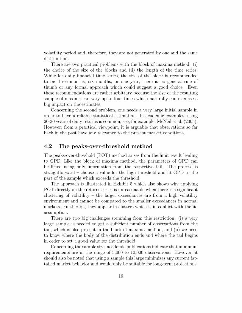
The approach is illustrated in Exhibit 5 which also shows why applyingPOT directly on the returns series is unreasonable when there is a significantclustering of volatility – the larger exceedances are from a high volatilityenvironment and cannot be compared to the smaller exceedances in normalmarkets. Further on, they appear in clusters which is in conflict with the iidassumption.

There are two big challenges stemming from this restriction: (i) a verylarge sample is needed to get a sufficient number of observations from thetail, which is also present in the block of maxima method, and (ii) we needto know where the body of the distribution ends and where the tail beginsin order to set a good value for the threshold.

Concerning the sample size, academic publications indicate that minimumrequirements are in the range of 5,000 to 10,000 observations. However, itshould also be noted that using a sample this large minimizes any current fat-tailed market behavior and would only be suitable for long-term projections.

16

Exhibit 5: The daily losses of S&P500 from November 3, 2000 to November5, 2010 and the exceedances over a threshold of 3%.

For financial time series, where the standard time window for risk estimationis two years of daily data, a sample size of just 500 observations is far tooshort to ensure an accurate GPD fit. Goldberg et al. (2008) suggest 1,000days, with approaches to generate synthetic data where enough observationsare not available.

The second issue may seem easy to resolve by resorting to statistical meth-ods that would indicate where the tail begins. However, no reliable methodsof this type exist. Typically, this high threshold is chosen subjectively bylooking at certain plots, such as the Hill plot or the mean excess plot, whichare standard in EVT. As a consequence, identifying the threshold betweenthe body and the tail is a matter of subjective choice based on visual in-spection, which cannot be achieved on a large scale. Kuipers test has beensuggested in Goldberg et al. (2008) as a numerical method for determiningthe optimal threshold selection. However, this test is very difficult to au-tomate for large universes, because the resulting optimization problem doesnot have good optimality properties, with the global minimum being hardto find. The fact that the choice of this threshold has a great impact on theparameter estimates of GPD and, therefore, on the final risk estimates insmaller samples is acknowledged in Goldberg et al. (2008) and Castillo and

17

Daoudi (2008).In using GPD, one is always faced with the classical tail-estimation trade-

off problem. For the GPD estimates to be unbiased, they must be fit withthe largest possible threshold. Unbiased estimators are obtained when thethreshold is infinity. This implies that one should use a very small numberof extreme observations from the original sample. On the other hand, usingsuch a small number of observations drastically increases the variance of theestimators. GPD estimation fits become more of an art than a science inbalancing this trade-off between being unbiased and small variance of theestimators. It should be noted that fitting the parameters of GEV has thesame deficiencies, see Hull and Welsh (1985).

5 Model selection

Having discussed different classes of fat-tailed models which can account forthe observed fat-tailed behavior of asset returns, the pragmatic mind wouldbe interested in criteria for model selection. A few general rules can beconsidered which can eliminate inappropriate choices. First, models whichallow for fat-tailed representatives and also for light-tailed representativesare more appealing compared to models with a fixed tail thickness, e.g. theone suggested in Zumbach (2006). In this way, if the empirical tail is closeto normal the model would be able to recognize it. Rejecting a richer modelonly on the grounds of parsimony as argued in Esch (2010) makes sense onlyafter an extensive statistical analysis.

Second, choosing a model may depend on the particular problem we aretrying to solve. From a theoretical viewpoint, some models arise from limittheories in probability theory which make them suitable for some types ofproblems. Operational risk, for example, requires loss estimation deep inthe tail, e.g. VaR at the 99.9% level, which makes EVT-based models goodcandidates. They have to be applied carefully bearing in mind the caveatsmentioned in Section 4. Full distribution models are more appropriate inmarket risk estimation when the left tail of the portfolio return distributionis used in the calculation of multiple quantile levels some of which are notin the extreme tail, e.g. VaR at 95%, 99%, and 99.5%. Tempered stabledistributions represent an appealing choice for the residual process in a time-series model but other distributions can also be used.

Third, back-testing studies should be considered when choosing between

18

different models. They can identify certain models as overly optimistic oroverly pessimistic. Rachev et al. (2010) consider a back-testing of VaR at99% confidence level of DJIA in which Gaussian, Student’s t, stable and EVTmodels are compared after cleaning the clustering of volatility effect througha GARCH model. The back-testing study indicates that EVT and Student’st with the DOF parameter fixed to 5 as suggested in Zumbach (2006) lead tooverly conservative VaR models. Not surprizingly, the Gaussian model, onthe other hand, turns out to be overly optimistic. Additional analysis and acomparison in a more simplified setting is available in Marinelli et al. (2007).

Having selected a distributional model, one has to calculate confidenceintervals of the risk statistics through non-parametric bootstrapping whichprovides a measure of sensitivity of the output of the model to the input sam-ple. The same exercise can be repeated with the parameters of the fat-taileddistribution which will provide insight into the variability of the estimator.If the Monte Carlo method is involved, then the Monte Carlo variability ofthe risk statistics has to be explored as well in order to tune the number ofgenerated scenarios. Studies of this type help identify factors that may causeinstabilities and situations in which the model may fail.

6 Conclusion

After the financial meltdown of 2008, it seems the existence of fat tails inasset returns and the importance of this phenomenon for downside portfoliorisk estimation is getting more widely recognized by practitioners. Academicliterature is abundant in models that can take into account fat tails butthis stylized fact should not be considered in isolation. A realistic model forasset returns should take into account all statistically relevant stylized facts.The best approach is to choose an extended model that includes the normaldistribution as a special case and then test its performance on the real data.The more theoretical question of whether the chosen model is the best oneamong all other families of fat-tailed models is not so essential as there may bedifferent families of fat-tailed distributions which are statistically equivalentas far as the particular modeling problem is concerned.

19

References

Akgiray, A. (1989), ‘Conditional heteroskedasticity in time series of stockreturns: evidence and forecast’, Journal of Business 62, 55–80.

Bhansali, V. (2008), ‘Tail risk management’, Journal of Portfolio Manage-ment 34(4), 68–75.

Bianchi, M. L., S. T. Rachev, Y. S. Kim and F. J. Fabozzi (2010), ‘Temperedinfinitely divisible distributions and processes’, Theory of Probability andIts Applications 55(1), 59–86.

Blattberg, R. C. and N. J. Gonedes (1974), ‘A comparison of the stableand student distributions as statistical models for stock prices’, Journal ofBusiness 47, 244–280.

Campbell, R., C. Forbes, K. Koedijk and P. Kofman (2008), ‘Increasingcorrelations or just fat tails?’, Journal of Empirical Finance 15(2), 287–309.

Castillo, J. Del and J. Daoudi (2008), ‘Estimation of the generalized paretodistribution’, Statistics & Probability Letters 79(5), 684688.

Dubikovsky, V., M. Hayes, L. Goldberg and M. Liu (2010), ‘How well can therisk of financial extremes be forecast?’, Whitepaper, MSCI Barra, ResearchInsights .

Eberlein, E. and U. Keller (1995), ‘Hyperbolic distributions in finance’,Bernoulli 1(3), 281–299.

Embrechts, P., C. Kluppelberg and T. Mikosch (1997), Modeling extremalevents for insurance and finance, Springer.

Esch, D. (2010), ‘Non-normality facts and fallacies’, Journal of InvestmentManagement 8(1), 49–61.

Fama, E. (1963), ‘Mandelbrot and the stable paretian hypothesis’, Journalof Business 36, 420–429.

Fama, E. (1965), ‘The behavior of stock market pricess’, Journal of Business38, 34–105.

20

Goldberg, L., G. Miller and J. Weinstein (2008), ‘Beyond value at risk: Fore-casting portfolio loss at multiple horizons’, Journal of Investment Manage-ment 6(2), 73–98.

Hull, P. and A. Welsh (1985), ‘Adaptive estimates of parameters of regularvariation’, Annals of Statistics 122(1), 331341.

Kim, Y. S., S. T. Rachev, M. L. Bianchi and F. J. Fabozzi (2008), ‘Financialmarket models with Levy processes and time-varying volatility’, Journalof Banking and Finance 32(7), 1363–1378.

Kim, Y., S. T. Rachev, M. L. Bianchi and F. J. Fabozzi (2010), ‘Temperedstable and tempered infinitely divisible GARCH models’, Journal of Bank-ing and Finance 34, 2096–2109.

Kon, S. (1984), ‘Models of stock returns - a comparison’, Journal of Finance39, 147–165.

Mandelbrot, B. (1963), ‘The variation of certain speculative prices’, Journalof Business 26, 394–419.

Marinelli, C., S. D’Addona and S. Rachev (2007), ‘A comparison of someunivariate models for value-at-risk and expected shortfall’, InternationalJournal of Theoretical and Applied Finance 10(6), 1043–1075.

Martellini, L. and V. Ziemann (2010), ‘Improved estimates of higher-ordercomoments and implications for portfolio selection’, Review of FinancialStudies 23(4), 1467–1502.

McNeil, A., R. Frey and P. Embrechts (2005), Quantitative risk management:Concepts, techniques and tools, Princeton University Press.

Mittnik, S. and S. Rachev (1993), ‘Modelling asset returns with alternativestable distributions’, Econometric Reviews 12(3), 261–230.

Rachev, S., B. Racheva-Iotova and S. Stoyanov (2010), ‘Capturing fat tails’,Risk Magazine May 2010, 72–77.

Rachev, S.T. and S. Mittnik (2000), Stable Paretian Models in Finance, JohnWiley & Sons, Series in Financial Economics.

21

Samorodnitsky, G. and M. Grabchak (2010), ‘Do financial returns have finiteor infinite variance? a paradox and an explanation’, Quantitative Finance.

Sheikh, A. Z. and H. Qiao (2009), ‘Non-normality of market returns: Aframework for asset allocation decision making’, Whitepaper, J.P. MorganAsset Management, JPMorgan Chase & Co .

Zumbach, G. (2006), ‘A gentle introduction to the RM2006 methodology’,RiskMetrics Technology Paper .

22

No. 30

No. 29

No. 28

No. 27

No. 26

No. 25

No. 24

No. 23

No. 22

No. 21

No. 20

No. 19

Stoyan V. Stoyanov, Svetlozar T. Rachev, Boryana Racheva-Iotova, Frank J.

Fabozzi: Fat-tailed models for risk estimation, May 2011

Stoyan V. Stoyanov, Svetlozar T. Rachev, Frank J. Fabozzi: CVaR sensitivity

with respect to tail thickness, May 2011

Young Shin Kim, Svetlozar T. Rachev, Michele Leonardo Bianchi, Frank J.

Fabozzi: Tempered stable and tempered infinitely divisible GARCH

models, May 2011

Takashi Kanamura, Svetlozar T. Rachev, Frank J. Fabozzi: A profit model

for spread trading with an application to energy futures, May 2011

Michele Leonardo Bianchi, Svetlozar T. Rachev, Young Shin Kim, Frank J.

Fabozzi: Tempered infinitely divisible distributions and processes, May

2011

Sebastian Kube, Michel André Maréchal and Clemens Puppe: The

currency of reciprocity - gift-exchange in the workplace, April 2011

Clemens Puppe and Attila Tasnádi: Axiomatic districting, April 2011

Dinko Dimitrov and Clemens Puppe: Non-bossy social classification, April

2011

Kim Kaivanto and Eike B. Kroll: Negative recency, randomization device

choice, and reduction of compound lotteries, April 2011

Antje Schimke and Thomas Brenner: Long-run factors of firm growth - a

study of German firms, April 2011

Aaron B. Scholz: Spatial network configurations of cargo airlines, April

2011

Arne Beck: Public bus transport in Germany - a proposal to improve the

current awarding system, April 2011

recent issues

Working Paper Series in Economics

The responsibility for the contents of the working papers rests with the author, not the Institute. Since working papers

are of a preliminary nature, it may be useful to contact the author of a particular working paper about results or ca-

veats before referring to, or quoting, a paper. Any comments on working papers should be sent directly to the author.