fault attacks and countermeasures
TRANSCRIPT

Dissertation
Fault Attacks and Countermeasures
Martin Otto
Fakultat fur Elektrotechnik, Informatik und Mathematik
Institut fur Informatik
Universitat Paderborn
Betreuer: Prof. Dr. Johannes Blomer
Dezember 2004

ii
Fault Attacks and Countermeasures

iii
for my parents
Martin Otto, Dissertation, December 2004

iv
Fault Attacks and Countermeasures

v
Acknowledgments
During the course of writing my Ph.D. thesis, many people have been supporting me and mywork, and this thesis is a good opportunity to express my gratitude for them.
First of all, I would like to thank my supervisor, Prof. Dr. Johannes Blomer, for his greatsupport. He introduced me to the very interesting field of fault attacks and showed me in manyhelpful discussions how to improve my work and suggested in which direction my research shouldgo. The atmosphere in his research group was very creative. In particular, Johannes offered methe opportunity to do the work in my own style and time.
I would also like to thank Prof. Dr. Joachim von zur Gathen, who has been my secondsupervisor in the PaSCo graduate school, and who introduced me to the field of cryptography.Additionally, I would like to thank Dr. Jean-Pierre Seifert from Intel, with whom I cooperatedclosely. He provided great insight in various problems and was a great help in understanding thepractical issues of cryptography on smartcards from the viewpoint of commercial applications.
Then I would like to thank Valentina Damerow, Thomas Leyer, Mirko Hessel-von Molo andDr. Alexander May for carefully reading parts of my thesis and helping me improve its qualitywith many valuable comments.
I enjoyed the friendly and relaxed atmosphere at my work place, both in the research group ofJohannes and in the research group of Prof. Dr. Friedhelm Meyer auf der Heide, and especiallyworking together with the office crew, Sabrina Geissler, Birgitta Grimm, Marcel R. Ackermann,Tobias Selms, and Dirk Pommerenke. I have to thank Oliver Vogel for writing X-Blast, whichserved perfectly as an opportunity for short distractions.
My research was made possible by two grants, for which I am very thankful. First, I wasa member of the DFG graduate school No. 693 “Scientific Computation: Application-orientedModelling and Development of Algorithms”, hosted by the Paderborn Institute for ScientificComputation (PaSCo). Here, my work was supported beyond financial coverage by the inter-disciplinary environment of a graduate school with people from several different countries. Thisoffered some great opportunities to present and discuss my work with people from differentscientific areas. In the last phase of my research, I received a grant from the University ofPaderborn, allowing me to finish my thesis.
I would also like to thank a bunch of people for support during various stages of my time atthe University of Paderborn, especially Barbara Fritsch, the people from ”mafia”, and MarcusNachtkamp, who created the birds.
Last, but not least, I would also like to thank my family, who has been a great support duringall times.
I had a lot of fun doing research at the University of Paderborn and especially in the field offault attacks. I hope the reader will sense some of the enthusiasm while reading this thesis.
Martin OttoPaderborn, December 2004
Martin Otto, Dissertation, December 2004

vi
Fault Attacks and Countermeasures

Contents
Introduction xi
1. Fault Attacks and Fault Models 1
1.1. Inducing Faults in the Physical World . . . . . . . . . . . . . . . . . . . . . . . . 2
1.1.1. Countermeasures . . . . . . . . . . . . . . . . . . . . . . . . . . . . . . . . 6
1.2. Characterizing Fault Models . . . . . . . . . . . . . . . . . . . . . . . . . . . . . . 7
1.3. Definition of Fault Types . . . . . . . . . . . . . . . . . . . . . . . . . . . . . . . 9
1.4. Definition of Fault Models . . . . . . . . . . . . . . . . . . . . . . . . . . . . . . . 12
1.4.1. Fault Models Affecting a Single Bit . . . . . . . . . . . . . . . . . . . . . . 14
1.4.2. Fault Models Affecting a Bounded Number of Bits . . . . . . . . . . . . . 16
1.4.3. Fault Models Affecting an Arbitrary Number of Bits . . . . . . . . . . . . 19
1.5. Validity and Applicability of the Proposed Fault Models . . . . . . . . . . . . . . 22
1.6. Other Attack Scenarios . . . . . . . . . . . . . . . . . . . . . . . . . . . . . . . . 24
1.6.1. Code Change Attacks . . . . . . . . . . . . . . . . . . . . . . . . . . . . . 24
1.6.2. Oracle Attacks . . . . . . . . . . . . . . . . . . . . . . . . . . . . . . . . . 24
2. New Attacks on Plain RSA 29
2.1. The Differential Fault Attack on Right-To-Left Repeated Squaring . . . . . . . . 30
2.1.1. Flaws in the Plain RSA Attack . . . . . . . . . . . . . . . . . . . . . . . . 33
2.1.2. Correcting Algorithm 2.5 and Lemma 2.7. . . . . . . . . . . . . . . . . . . 35
2.2. An Attack on The Left-To-Right Repeated Squaring Algorithm . . . . . . . . . . 45
2.2.1. Fault Attack Starting From the MSBs . . . . . . . . . . . . . . . . . . . . 47
2.2.2. Fault Attack Starting From the LSBs . . . . . . . . . . . . . . . . . . . . 56
2.3. Concluding Remarks and Open Problems . . . . . . . . . . . . . . . . . . . . . . 70
3. A New Countermeasure Against Attacks on CRT-RSA 73
3.1. CRT-RSA and the Bellcore Attack . . . . . . . . . . . . . . . . . . . . . . . . . . 73
3.2. Countermeasures . . . . . . . . . . . . . . . . . . . . . . . . . . . . . . . . . . . . 78
3.2.1. Infective Errors . . . . . . . . . . . . . . . . . . . . . . . . . . . . . . . . . 79
3.3. A New Countermeasure Against Random Faults . . . . . . . . . . . . . . . . . . 84
3.3.1. Efficiency Of The New Algorithm . . . . . . . . . . . . . . . . . . . . . . . 86
3.4. Security Analysis of the Proposed Countermeasure . . . . . . . . . . . . . . . . . 87
3.4.1. Undetectable Errors. . . . . . . . . . . . . . . . . . . . . . . . . . . . . . . 87
3.4.2. Excluding the Two Messages m = 0 and m = 1. . . . . . . . . . . . . . . . 92
3.4.3. Further Security Considerations . . . . . . . . . . . . . . . . . . . . . . . . 93
3.4.4. Summarizing the Results. . . . . . . . . . . . . . . . . . . . . . . . . . . . 94
3.5. Adapting to Other Fault Models . . . . . . . . . . . . . . . . . . . . . . . . . . . 94
3.5.1. Undetectable Faults in the Single Bit Fault Model . . . . . . . . . . . . . 94
vii

viii Contents
3.5.2. Undetectable Faults in the Byte Fault Model . . . . . . . . . . . . . . . . 97
3.6. Attacks Against our Proposed Algorithm . . . . . . . . . . . . . . . . . . . . . . 98
3.6.1. Bit and Byte Faults . . . . . . . . . . . . . . . . . . . . . . . . . . . . . . 98
3.6.2. Wagner’s Attack . . . . . . . . . . . . . . . . . . . . . . . . . . . . . . . . 100
3.7. Concluding Remarks and Open Problems . . . . . . . . . . . . . . . . . . . . . . 101
4. Fault Attacks on Elliptic Curve Cryptosystems 103
4.1. Elliptic Curve Cryptography . . . . . . . . . . . . . . . . . . . . . . . . . . . . . 103
4.1.1. Affine Coordinates . . . . . . . . . . . . . . . . . . . . . . . . . . . . . . . 104
4.1.2. Projective Coordinates . . . . . . . . . . . . . . . . . . . . . . . . . . . . . 106
4.1.3. Elliptic Curve Cryptosystems . . . . . . . . . . . . . . . . . . . . . . . . . 107
4.1.4. Elliptic Curve Parameters in Practice . . . . . . . . . . . . . . . . . . . . 108
4.2. Existing Fault Attacks on Elliptic Curve Cryptosystems . . . . . . . . . . . . . . 108
4.3. Undetectable Faulty Points in Point Addition . . . . . . . . . . . . . . . . . . . . 111
4.3.1. Examples for a Detailed Analysis of Undetectable Errors . . . . . . . . . . 112
4.4. Attacks Inducing Undetectable Faults . . . . . . . . . . . . . . . . . . . . . . . . 115
4.4.1. Faults Induced into Point Addition Using Random Faults . . . . . . . . . 115
4.4.2. Faults Induced into Point Addition Using Bit Faults . . . . . . . . . . . . 116
4.5. Sign Change Faults . . . . . . . . . . . . . . . . . . . . . . . . . . . . . . . . . . . 117
5. Sign Change Faults — Attacking Elliptic Curve Cryptosystems 123
5.1. Sign Change Attack on NAF-based Left-to-Right Repeated Doubling . . . . . . . 124
5.1.1. Sign Change Attack Targeting Q′i in Line 4. . . . . . . . . . . . . . . . . . 125
5.1.2. Other Attacks . . . . . . . . . . . . . . . . . . . . . . . . . . . . . . . . . 131
5.1.3. Recovering The Bits Starting From The MSB . . . . . . . . . . . . . . . . 132
5.2. Sign Change Attack on NAF-based Right-to-Left Repeated Doubling . . . . . . . 135
5.2.1. Sign Change Attack Targeting Qi in Line 4. . . . . . . . . . . . . . . . . . 135
5.2.2. Other Attacks . . . . . . . . . . . . . . . . . . . . . . . . . . . . . . . . . 136
5.2.3. Recovering The Bits Starting From The MSB . . . . . . . . . . . . . . . . 138
5.3. Attacks on the Standard Repeated Doubling Algorithms . . . . . . . . . . . . . . 138
5.4. Sign Change Attack on Montgomery’s Binary Method . . . . . . . . . . . . . . . 138
5.4.1. Preliminaries . . . . . . . . . . . . . . . . . . . . . . . . . . . . . . . . . . 139
5.4.2. Sign Change Attack Targeting P1(i+1) . . . . . . . . . . . . . . . . . . . . 141
5.4.3. False Positives . . . . . . . . . . . . . . . . . . . . . . . . . . . . . . . . . 144
5.4.4. Other Attacks . . . . . . . . . . . . . . . . . . . . . . . . . . . . . . . . . 149
5.4.5. Recovering The Bits Starting From The MSB . . . . . . . . . . . . . . . . 152
5.5. Concluding Remarks . . . . . . . . . . . . . . . . . . . . . . . . . . . . . . . . . . 155
6. Securing Elliptic Curve Cryptosystems 157
6.1. Previously Proposed Countermeasures . . . . . . . . . . . . . . . . . . . . . . . . 157
6.2. A New Countermeasure Against Sign Change Attacks . . . . . . . . . . . . . . . 158
6.2.1. On the Choice of Ep and Et. . . . . . . . . . . . . . . . . . . . . . . . . . 159
6.2.2. Analysis of the Countermeasure. . . . . . . . . . . . . . . . . . . . . . . . 160
6.2.3. Infective Computations . . . . . . . . . . . . . . . . . . . . . . . . . . . . 163
Fault Attacks and Countermeasures

Contents ix
7. Sign Change Attacks — RSA Revisited 1657.1. Sign Change Faults in Left-to-Right Repeated Squaring . . . . . . . . . . . . . . 1667.2. Sign Change Faults in Right-to-Left Repeated Squaring . . . . . . . . . . . . . . 166
8. Conclusion and Open Problems 169
A. Detailed Fault Analysis of Affine Elliptic Curve Addition 171A.1. Attacks Targeting λ = (y1 − y2)/(x1 − x2) . . . . . . . . . . . . . . . . . . . . . . 171A.2. Attacks Targeting x3 = λ2 − x1 − x2 . . . . . . . . . . . . . . . . . . . . . . . . . 175A.3. Attacks Targeting y3 = −y1 + λ · (x1 − x3) . . . . . . . . . . . . . . . . . . . . . . 177
Bibliography 181
Symbols, Acronyms and Notation 189
Martin Otto, Dissertation, December 2004

List of Figures
1. Black Box Assumption . . . . . . . . . . . . . . . . . . . . . . . . . . . . . . . . . xiv2. Real World Assumption . . . . . . . . . . . . . . . . . . . . . . . . . . . . . . . . xvi
1.1. Assignment of the contacts of a smartcard as defined in ISO 7816-2 [ISO02a]. . . 41.2. Architectural sketch of a modern high-end smartcard. . . . . . . . . . . . . . . . 13
4.1. The elliptic curve y2 = x3 − 15 · x + 20. . . . . . . . . . . . . . . . . . . . . . . . 1034.2. Point addition on an elliptic curve. . . . . . . . . . . . . . . . . . . . . . . . . . . 105
List of Tables
1.1. Parameters and their possible values characterizing fault models . . . . . . . . . 91.7. Overview of the fault models defined in Section 1.4 . . . . . . . . . . . . . . . . . 23
3.6. Summarizing the success probabilities of a fault attack adversary . . . . . . . . . 943.7. Summarizing the success probabilities of a fault attack adversary for bit faults . 973.8. Summarizing the success probabilities of a fault attack adversary for byte faults . 97
4.1. Recommended Elliptic Curve Parameters . . . . . . . . . . . . . . . . . . . . . . 1094.2. Size of system parameters and key pairs (approx.) from [Cer00] . . . . . . . . . . 109
x

Introduction
Exchanging messages securely between two parties, without allowing a third party to wiretapthe conversation, is a problem, which is thousands of years old. It has been addressed by cryp-tography, i.e., by encrypting messages, as early as in ancient Egypt around 1900 B.C., wherea scribe used non-standard hieroglyphs in an inscription [Sch00b, p. 86]. The ancient idea ofencrypting messages is to use symmetric encryption, i.e., a cryptosystem where both communi-cating parties share the same secret key. Obviously, this common key has to be exchanged safelyat some time, which is a major problem when communicating with people over large distances.Using cryptography has long been too cumbersome to be deployed beyond intelligence agenciesand the military.
However, in 1976, Whitfield Diffie and Martin Hellman [DH76] came up with a new directionin cryptography: asymmetric cryptosystems. Asymmetric cryptosystems, or public key cryp-tosystems, allow to use two different keys, a public key and a private key. The public key issolely used for encrypting a message. Decrypting a ciphertext cannot be done with the publickey. To decrypt a ciphertext, the secret key must be known. If it is infeasible to computethe secret key from the public key, the public key may be published freely. This solves theproblem of exchanging the keys, which prevented widespread use of symmetric cryptosystems.Consequently, this revolution in cryptography triggered the use of cryptography in numerousapplications. Nowadays, cryptography is at the core of everyday life, securing almost all aspectsof, e.g., communication via the internet, e-commerce, and online banking. It is a crucial corner-stone, which makes the global economy, and especially the internet work. There is subtle ironyin the fact that making information public solves major problems of exchanging secret messages.
The basic principle of asymmetric cryptosystems are one-way functions. A one-way functionis a function, which is easy to compute, but computationally infeasible to invert. Computing aone-way function corresponds to encrypting a message, and inverting the function correspondsto decrypting a ciphertext. However, to make decryption possible, the secret key serves as addi-tional knowledge, which allows to invert a one-way function easily. Such additional knowledgeis referred to as a trapdoor, and such a one-way function as a trapdoor one-way function. Thesefunctions are the underlying structure of every public key cryptosystem.
xi

xii Introduction
In 1978, Ronald Rivest, Adi Shamir, and Leonard Adleman [RSA78] proposed the first publickey cryptosystem: RSA. The RSA encryption function is based on modular exponentiationmodulo a composite number N = p ·q, where p and q are primes. A message m is exponentiatedwith a public key e to yield a ciphertext c = me mod N . Given the secret key d, the ciphertextcan be decrypted by computing m ≡ cd mod N . It should be mentioned that asymmetriccryptography as well as the RSA cryptosystem had already been developed a few years earlierby James Ellis, Clifford Cocks, and Malcolm Williamson, however, they worked for a secretBritish agency named GCHQ and were not allowed to publish their results [Sch00b]. Othercryptosystems have been proposed thereafter, e.g., the ElGamal cryptosystem [ElG85], which isbased on the discrete exponentiation function in groups, e.g., the group of points on an ellipticcurve. The RSA and the ElGamal cryptosystems are described in detail in Protocol 2.1 andProtocol 4.3, respectively.
It has not been proved by anyone, that the RSA encryption function really is a trapdoorone-way function. And even worse: it is not known whether one-way functions exist at all.Still, public key cryptosystems are being used extensively with the help of functions, which arecandidate one-way functions, i.e., functions, which are hoped to be and which are generallyassumed to be one-way functions.
The RSA cryptosystem has survived more than 25 years of attacks. While details had to beadjusted, the basic idea of the RSA cryptosystem is still unbroken, and the RSA system is usedextensively today. Hence, it is reasonable to put some confidence in the believe, that the RSAencryption function as used today is a very good candidate for a one-way function.
Asymmetric Cryptography and Digital Signatures
The security of modern cryptography relies on various unproved assumptions. In this thesis, wewill show that some of these assumptions do not hold in practice. This observation allows fornew and partly devastating attacks, and this thesis aims to add knowledge to this field.
In this thesis, we focus on digital signature schemes. In principle, many public key cryptosys-tem can also be used as a digital signature scheme. Here, one party, named Alice, decrypts amessage using her secret key to obtain a digital signature. Then, another party, named Bob,can verify the signature by encrypting the digital signature with the public key. If the result isequal to the message, the message is believed to be authentic.
Secure digital signatures are a second major area of modern cryptography. They have beenmotivated by the needs of commerce and communication via the internet. If two parties want toagree on a contract via the internet, both have to sign the contract. A digital signature schemecan be used to provide authentication of data, data integrity, and non-repudiation. Moreover,applicability in the real world requires that digital signatures are also recognized by courts.Today, digital signature schemes exist, which can be used as a legal alternative for handwrittensignatures, i.e., as specified by the German Signaturgesetz [Sig01a], [Sig01b]. However, theirsecure use must be guaranteed. And guaranteeing security is all but an easy problem.
Security of Modern Cryptosystems: The Standard Approach
Let us first review the standard terms, in which security of a cryptosystem used for digitalsignatures is measured. Here, three aspects are considered. First, one has to define the objectiveof an adversary, e.g., what the goal of his attack is. Second, one has to agree on some model,in which security is defined, i.e., a model to measure security. And third, one has to define the
Fault Attacks and Countermeasures

Introduction xiii
power of the adversary, i.e., what kind of attacks he is able to mount on a system. Given thesethree aspects, researchers try to prove that a certain adversary cannot achieve a specific goalwith respect to some notion of security. Upon existence of such a proof, a system is considered tobe secure. Since we are mainly concerned with signature schemes in this thesis, we will describeall these aspects in terms of digital signatures.
Objectives. For a signature scheme, an adversary may have one of three different objectives.First, he might want to achieve a total break of the system. Here, he wants to recover the secretkey, which enables him to sign any arbitrary message and to act as the legitimate signer withoutany chance of distinguishing between them. Second, he could be satisfied with a selective forgery.A selective forgery means that if the adversary is given a message m, he is able to compute avalid signature for this message. This does not need to imply that the adversary recovers thesecret key. And third, as the weakest goal an adversary might have, there is existential forgery.Here, an adversary’s objective is to compute a pair (m, s), such that m is a message and s isthe valid signature of that message m. The message m might not be selectable by the adversaryand might not represent any meaningful text. The total break is the strongest objective, whilethe existential forgery is the weakest objective.
Models of Security. A naive approach to security would demand that a signature scheme issecure if the weakest objective, i.e., existential forgeries, is impossible to achieve by the strongestadversary possible. However, this approach is not practical. It is clear that for any valid message,a valid signature exists, hence, an adversary can always construct valid message/signature pairsby simply guessing the signature with some non-zero probability. Hence, the best thing to proveis that an adversary’s success probability is not significantly higher than the probability that arandomly chosen signature is a valid signature of a given message. In practice, the following twomodels of security are considered for public key cryptosystems, although others exist as well (cf.[MvOV96]).
The most practical model of security is computational security. To have confidence in thesecurity of a proposed cryptosystem, it should be computationally secure. For this notion ofsecurity, an adversary is assumed to have limited resources, i.e., time and memory polynomialin the input parameters. Security is based on the fact that the problem of breaking a systemis related to solving a problem, which is assumed to be computationally hard. Here, “hard”does usually not represent NP-hard, but the assumed hardness of a well-studied problem. Forexample, some popular systems are reduced to the integer factorization problem (e.g., RSA)or the discrete logarithm problem (e.g., ElGamal). However, simply reducing the problemof breaking a system to solving some hard problem is not enough. It is desired, that the twoproblems are computationally equivalent. If this can be shown, a cryptosystem is called provablysecure. Both, the RSA cryptosystem and the ElGamal cryptosystem exist in provably securevariants, which depend on different assumptions about the hardness of some problems.
Another possible model of security is ad-hoc security. Here, security only relies on extensiveresearch and heuristics. No security is guaranteed, yet, if a large number of researchers tried tobreak a cryptosystem for a significant amount of time, if it is secure against standard attacks,and if there are good arguments why breaking the system should be computationally infeasible,one might be tempted to trust the cryptosystem. However, here is no proof and the systemcould be broken the very next day by some clever and new idea.
Martin Otto, Dissertation, December 2004

xiv Introduction
Attack Models. In a signature scheme, it is general consensus that an adversary always hasboth, access to all data being transmitted by two communicating parties and exact knowledgeof every aspect of the used signature scheme, with the only exception of the secret key. Hence,the security of a system must rely on the secret key only. An adversary might also be ableto eavesdrop on a conversation with many signed messages being exchanged. This situation iscaptured in an attack model named an adaptive chosen message attack. Here, the knowledge ofthe adversary about various pairs of messages and valid signatures is modeled by the assumptionthat an adversary has access to a signature oracle. An adversary can request signatures ofpolynomially many (in the size of the input parameters) chosen messages to achieve his objective.He may choose the messages to be signed adaptively, i.e., based on all message/signature pairscollected before. Obviously, in order to achieve a forgery, he must be able to construct a new,previously unseen message/signature pair. Any practical system should be secure against suchan adversary. It might be argued that for some special setups, an adaptive chosen message attackis impossible. In this case, weaker attack models exist (see [MvOV96, § 11.14] for details).
The basic assumption about an adversary is a harsh restriction on his knowledge. In allattack models, the adversary is limited to knowledge of a certain number of input/output pairs,i.e., message/signature pairs, and knowledge about the specification and implementation ofthe cryptographic protocol (the latter is usually referred to as Kerckhoffs’ Assumption). Thisscenario is a black-box assumption, depicted in Figure 1. It allows purely theoretical proofs onpaper, without having an algorithm implemented, without having to actually use a system.
Input - Encrypt/Sign - Output
Figure 1.: Black Box Assumption
Given the black-box approach, numerous cryptosystems can be proved to be secure. However,what is the practical relevance of such a proof? If you consider a cryptosystem alone in avacuum, you would probably be fine with such a security proof. However, imagine that thissystem is not used in a well defined mathematical environment, but in the real world. Here,cryptographic protocols are implemented on computers, which adhere to the laws of physics.Would you still be confident?
Security of Modern Cryptosystems: Getting Real
Cryptographic protocols are used in the real world, and this has severe implications for the term“security”. In the real world, cryptosystems have to be implemented using some programminglanguage or hardware circuits, which have to be run on some sort of computer, and humanbeings use it. Therefore, cryptography does not exist in a vacuum and security does not onlydepend on mathematical properties. In real life, an adversary has a lot of possibilities to breaka “provable secure” cryptosystem.
Real World Attacks. In the real world, an adversary can go beyond the mathematical conceptand attack the implementation rather than the specification. Obviously, the real world offersmany possibilities for attacks, which cannot be modeled or prevented by mathematics. Forexample, an adversary could force the legitimate owner to disclose his secret key. Or, he could
Fault Attacks and Countermeasures

Introduction xv
exploit the fact that today’s secret key lengths are far beyond the abilities of humans to memorizethem. Hence, a 2048 bit RSA key would be stored somewhere and would be protected with, say,an 8-letter password. Here, an adversary could hope that the password is chosen as the nameof the husband or wife of the legitimate owner. Or, an adversary can hope that a programmer,implementing a mathematical concept in some programming language, uses unsecured sharedmemory to store the secret key. Or, he could try to transmit a virus or a trojan horse on a userscomputer, which dumps the memory content while a cryptographic application reads the secretkey.
The given examples show that security in the real world depends on some assumptions, cryp-tographers silently agree on. First, it is assumed that all parties play by the rules and follow thespecification. This is a reasonable assumption. However, it is also assumed that a cryptosystemrunning on some device cannot be attacked by other means than described by the black boxmodel. This assumption is not realistic. One major problem for security in the real world is theenvironment, in which a cryptographic algorithm is executed. The device running an algorithm,as well as the operating system, must represent a safe harbor. A cryptographic protocol cannotbe secured against a hostile operating system, which analyzes the code while it is executed.
Now, it is common perception that personal computers are all but secure platforms. Theextensive occurrence of viruses, worms, and trojan horses shows that a desktop computer caneasily be compromised. This implies that cryptographic applications cannot be guaranteed tobe secure if run on an ordinary computer. However, signature schemes, which are intended to beused as a legal alternative to handwritten signatures, must be guaranteed to achieve a certainlevel of security (cf. [Sig01a], [Sig01b]). This triggered the use of dedicated and specially securedhardware for cryptographic purposes, especially for digital signatures.
Using Smartcards. Smartcards have long been considered as an ideal environment for digitalsignature schemes. They do not offer any possibility to have new code or updates being loadedonto them, hence viruses and other malicious code are no longer a problem. Moreover, smart-cards have a significant computational power if compared to their size. Modern smartcards arefaster and have more memory than a C64 standard computer used in the 1980s. Hence, evencryptographic schemes, which involve a significant amount of arithmetic operations, e.g., ellipticcurve cryptosystems, can be run on them. There is no need to hope for a friendly operatingsystem, since the complete system is provided by the manufacturer, including the hardware. Asmartcard is designed for the only purpose of a specific task. This makes it easier to test asystem thoroughly for bugs and other weaknesses. Moreover, smartcards are small and easy tocarry around, which makes them highly attractive, since they ease the use of digital signaturesin everyday life. Hence, smartcards seem like an ideal environment for digital signature schemes.
Side-Channels. However, smartcards are electronic devices. They must obey the laws ofphysics. Hence, if a smartcard computes a result, it requires a certain amount of time anda certain amount of energy, the electronic circuits emit a certain amount of radiation, energy,and even sound, and they may be affected by their environment. Since smartcards are notequipped with an own power source or an own clock signal generator, they have to be connectedto a smart card reader. This reader can easily measure, e.g., time and power consumption ofthe smartcard. If any of this data is somehow correlated to secret data — and this is of coursethe case for digital signature computations — an adversary gets additional information. Thissituation is not captured by the black box model depicted in Figure 1. These additional sourcesof information are referred to as side-channels. Reality cannot be modeled as a black box, it only
Martin Otto, Dissertation, December 2004

xvi Introduction
allows for a “gray box”, where an adversary has access to several side-channels. This situationis captured in Figure 2.
Input - Encrypt/Sign - Output
? side channels ?
Figure 2.: Real World Assumption
It has been shown by various authors that a large number of these side-channels provideinformation, which reveals important and compromising details about secret data. Some ofthese details can be used as new trapdoors to invert a trapdoor one-way function withoutthe secret key. This allows an adversary to break a cryptographic protocol, even if it provedto be secure in the classical, mathematical sense. The various side-channels include timingmeasurements ([Koc96b]), power consumption and the power profile ([KJJ99]), electromagneticemissions ([QS01], [RR01], [GMO01]), sound ([ST04]), presence and abuse of testing circuitry([Koc96a], [YWK04]), data gathered by probing circuitry or bus lines ([HPS99]), cache memorybehaviour ([Pag02]), and faults ([AK96], [BDL97]). Research in side-channel attacks is still avivid area of research, hence, additional side-channels may be discovered on a daily basis.
Fault Attacks. This thesis concentrates on one specific side-channel: faults. Here, an adversaryinduces faults into a device, while it executes a known program, and while the adversary observesthe reaction. These attacks are named fault attacks, and they are fundamentally different fromother side-channel attacks. Other side-channel attacks are passive attacks, which just listen tosome side-channel without interfering with the computation. Fault attacks are active attacks,where an adversary has to tamper with an attacked device in order to create faults, therebyopening the desired side-channel. Smartcards have long been considered to be tamper-proofdevices, until an article by Ross Anderson and Markus Kuhn [AK96] suggested that smartcardsmay at most be tamper-resistant, but definitely not tamper-proof. If an adversary can inflictsome sort of physical stress on the smartcard, he can induce faults into the circuitry or memory.These faults become manifest in the computation as errors. If an error occurs, a faulty finalresult is computed. If the computation depends on some secret key, a comparison betweencorrect data and faulty data may allow to conclude facts about the secret key.
The first successful fault attacks have been reported by Dan Boneh, Richard DeMillo, andRichard Lipton from Bellcore Labs in 1997 [BDL97]. They presented two important attacks onvariants of RSA, used for computing digital signatures. Their first attack targeted CRT-RSA,a fast variant of repeated squaring, which will be discussed in detail in Chapter 3 in this thesis.Here, a single faulty result may allow an adversary to completely break the given instance ofRSA. A second attack on RSA targeted repeated squaring. It is described in detail in Chapter2. Here, a secret key d of length n := l(d), where l(d) denotes the binary length of d, can berecovered with probability at least 1/2 given O(n log(n)) faulty signatures.
These results triggered extensive research in the field of fault attacks. In the following, severalauthors extended the ideas from Boneh, DeMillo, and Lipton to other cryptosystems, using otherfault models and different means of physical attacks. Chapter 1 will discuss known physicalattacks and fault models in greater detail. Some attacks, referred to as oracle attacks, do noteven need a faulty result at all, they deduct information about the secret key using only the
Fault Attacks and Countermeasures

Introduction xvii
information whether a fault changed the normal behaviour of a device or not. Fault attackshave been mounted successfully on symmetric and asymmetric cryptosystems alike, and theyhave even been used to break completely unknown ciphers [BS97]. Most fault attacks reportedso far are attacks, where an adversary needs to compare the final result to some known correctdata to verify that a fault occurred at all.
The Threat is Real. Fault attacks are a practical scenario. Fault attacks have been used tobreak security mechanisms even before the cryptographic community became aware of them.Pay TV card hackers used rapid transient changes in the clock signal, called clock glitches, toaccess pay TV channels before 1996 [AK97]. Other possible scenarios are easily sketched, whichshow that fault attacks are a real threat to smartcards. For example, imagine a customer usinghis signature smartcard in some Mafia shop, where the smartcard reader is provided by thehostile seller. In this case, the seller can attack the smartcard and induce faults even underthe eye of the customer, who only sees the reader. Since smartcards are fast, a seller can easilyattack the card a few times, before initiating the legitimate transaction. Obviously, by takinga stolen smartcard to a laboratory, an even wider variety of attacks is possible. Hence, faultattacks can be mounted on smartcards in reality.
Security Model. Since the threat of fault attacks is real, both customers and hardware manu-facturers are looking for secure smartcards. Here, two approaches are possible. First, hardwarecountermeasures can be applied to detect and prevent known methods of inducing faults, e.g.,detectors for clock glitches. Second, new algorithms can be developed, which are immune againstfault attacks.
Research in fault attacks is relatively new, with the first attacks having been reported in 1997[BDL97]. New attacks are still discovered frequently, and new physical attacks allow to inducefaults with an increasing variety of physical setups. Therefore, the scientific community has notyet been able to develop a theoretical framework to allow general security proofs for algorithmssupposedly secure against fault attacks. Some approaches have been made, but they are notsatisfying yet.
For passive side-channels, it is an obvious approach to ensure that the available information,e.g., the power profile, is independent of the secret key. A lot of countermeasures against variousattacks relying on power consumption traces, time measurements, or electromagnetic emissionmeasurements have been proposed, but it is still challenging to develop algorithms, which aresecure against all passive side-channel attacks. It happened often that a countermeasure intendedagainst one side-channel attack did not protect against another side-channel attack (e.g., [OS00],[Wal03], [OH03]), or even benefited another attack (e.g., [JQYY02], [YKLM01a], and a similarsituation will be described in Chapter 4 in this thesis). There have been some approaches tryingto unify the different passive side-channel attacks (e.g., [KW03]), and to develop a theoreticalframework (e.g., [JQYY02], [CJRR99]), [CKN00], [CCJ03], [MR04]). However, the issue ofprovable security for passive side-channel attacks is far from being settled.
For active attacks, i.e., fault attacks, the situation seems easier at first sight. If we assumethat an adversary can only induce a single fault, it is sufficient to run an algorithm threetimes on the same input and return the majority vote. This provides security against suchan adversary. However, this approach is not satisfying for practical applications, since it slowsdown a smartcard significantly. This is not acceptable in practice. Hence, new notions ofsecurity against fault attacks are desperately needed. There have been some approaches, e.g.,[Itk02], [Itk03], [MR04], and [Wag04], however, none of these models allows for an efficient
Martin Otto, Dissertation, December 2004

xviii Introduction
scheme, no practical scheme could be proved secure in these models. Nonetheless, algorithmiccountermeasures against fault attacks must be developed, which can be used in the real world.Until a suitable model for security against fault attacks has been developed, the best way to gois to show that a given scheme is secure against all known attacks. This resembles the ad-hocsecurity model defined for classic security analysis, and it is undoubtedly the weakest notion ofsecurity possible. However, this is the best notion available today.
Our Research. Our research, which culminated in this doctoral thesis, investigated fault at-tacks on asymmetric cryptosystems only. It was motivated by two goals: first, we were interestedin finding new fault attacks and new fault types, extending the attacks of Boneh, DeMillo, andLipton. However, fault attacks also establish the need for algorithms, which are secure againstthem. Therefore, as our second goal, we were searching for new algorithms, which are notsusceptible to fault attacks. We have been successful in both areas and present our results inthis dissertation. We present results for new attacks and for countermeasures for both, variantsof the RSA cryptosystem and variants of elliptic curve cryptosystems. For both of our coun-termeasures, we will prove the new algorithms to be secure against previously reported faultattacks.
Organization and Main Results
We briefly describe the organization of this thesis and present the main results.
Chapter 1. We start with a full characterization of fault models in Chapter 1. Here, we firstreview all physical attacks, which have been used successfully to induce faults into smartcards.Afterwards, we propose a new characterization for fault models as it is needed today. We describein detail the known fault types, the most important aspect of any fault model. Afterwards, wedefine five different fault models, which capture all reasonable fault models used in previousattacks. These definitions will be the basis for the remaining chapters.
Chapter 2. In Chapter 2, we present new results for fault attacks on plain RSA, i.e., onmodular exponentiation via repeated squaring. First, we start from the attack on plain RSA asintroduced by Boneh, DeMillo and Lipton in [BDL97]. We exhibit and correct two minor flawsin the original attack. Afterwards, we extend the original fault attack, which has been describedfor the right-to-left version of repeated squaring, to its twin version, the left-to-right repeatedsquaring algorithm. Here, we show that the bits of the secret key can be recovered both startingfrom the least significant bits, as well as starting from the most significant bits.
Chapter 3. A fast alternative to repeated squaring is the CRT-RSA algorithm, due to Chri-stophe Couvreur and Jean-Jacques Quisquater [CQ82]. Due to its advantage in speed, thisalgorithm is widely used on smartcards. However, it has been shown to be particularly suscep-tible to fault attacks like the “Bellcore attack” described in [BDL97]. In Chapter 3, we presenta new version of the CRT-RSA algorithm, which is secure against the Bellcore attack in themost realistic fault model. We will also show how the algorithm can be modified to be usedin stronger, less realistic fault models. The main results of this chapter have been published in[BOS03] as a joint work with Johannes Blomer and Jean-Pierre Seifert.
Fault Attacks and Countermeasures

Introduction xix
Chapter 4. After presenting attacks and countermeasures for the RSA cryptosystem in theprevious two chapters, we turn to elliptic curve cryptosystems in Chapter 4. We first introduceelliptic curves and review previously published attacks. We will show that contrary to previousbeliefs, it is possible to induce faults during the elliptic curve repeated doubling algorithm,which are not detected by the standard countermeasure proposed by different authors. Thiswill be shown by a brief but careful analysis of the error propagation during elliptic curve pointaddition. Since this analysis is rather technical, detailed results beyond instructive examples arepresented in Appendix A.
The results of the analysis give rise to a new fault type, Sign Change Faults. We end thechapter be defining this fault type and by describing how an adversary can induce faults of thistype. We show that this yields a new realistic fault model. Sign Change Faults are the basis forthe next three chapters.
Chapter 5. In Chapter 5, we use the new Sign Change Fault Model motivated by Chapter 4 forfault attacks on various versions of elliptic curve repeated doubling, i.e., left-to-right and right-to-left NAF-based repeated doubling, classic binary expansion-based repeated doubling, andMontgomery’s Binary Method. We will show that the basic scheme of fault attacks as describedin Chapter 2 can also be applied successfully to elliptic curve repeated doubling. Therefore, thenew fault model is a new threat for elliptic curve cryptosystems. Parts of the results presentedin this chapter have been published together with results from Chapter 6 in [BOS04] as a jointwork with Johannes Blomer and Jean-Pierre Seifert.
Chapter 6. Given the new sign change fault attacks presented in Chapter 5, a new secureversion of repeated doubling on elliptic curves is presented in Chapter 6. This countermeasureagainst Sign Change Faults seizes ideas already used successfully for the countermeasure againstfault attacks on CRT-RSA presented in Chapter 3. It can be used with any existing algorithmfor elliptic curve repeated doubling, which does not require field inversions. We show thatour new algorithm is secure against Sign Change Attacks and previously reported attacks. Thecountermeasure presented in this chapter has been published together with results from Chapter5 in [BOS04] as a joint work with Johannes Blomer and Jean-Pierre Seifert.
Chapter 7. In Chapter 7, we return to modular exponentiation and the RSA cryptosystem. Weshow that Sign Change Attacks are also a threat against the RSA cryptosystem. However, SignChange Attacks are much harder to realize for RSA type cryptosystems than for Elliptic Curvecryptosystems. Moreover, they are successful only against the right-to-left repeated doublingalgorithm.
Martin Otto, Dissertation, December 2004

xx Introduction
Fault Attacks and Countermeasures

1. Fault Attacks and Fault Models
Since the first report of a successful fault attack in [BDL97], many researchers have published re-sults about fault attacks. However, there have been few attempts for a unifying characterizationof fault models. Most researchers have implicitly assumed certain fault models, others have leftimportant details undefined. Therefore, in this section, we will present a full characterization offault models, as they need to be defined today.
Theoretically, an adversary may imagine any kind of error, e.g., that a device outputs thesecret key instead of the result of the computation. This may lead to the definition of anyfault model imaginable. Consequently, research in fault attacks established the habit that if acertain fault model is used, it is also described how such faults can be realized in the real world.Otherwise, the result may still be of mathematical interest, however, it does say little aboutthe security of today’s computers. In this view, research on fault attacks takes an engineeringpoint of view (cf. [YKLM01a]), since it is oriented by real devices and the real physical world.Therefore, it is crucial to motivate all fault models from the real world.
Consequently, we will start this section by reviewing the most important methods known tothe public to induce faults into devices, i.e., smartcards, in Section 1.1. This will show thatsuch methods are numerous. However, a mathematical view on inducing faults is needed forprofound theoretical analyses, to prove that attacks can recover secret information and break asystem, and to prove that algorithmic countermeasures really work. Hence, we need a theoreticalframework. This framework relies on carefully specified fault models. We will start with a fullcharacterization of fault models in Section 1.2. The most important aspect of any fault modelis the assumed fault type. Therefore, we devote a whole section, Section 1.3, to the discussionof all fault types used today in the open literature. Finally, in Section 1.4, we will define themost prominent fault models, which are used throughout the literature. These definitions willbe the basis for all results in the remaining chapters of this thesis.
Fault attacks can exploit faults in two different ways. One way is to cause the attackeddevice to malfunction and to output a faulty result. This result is then used to derive secretinformation. However, there are also fault attacks, which do not use the actual faulty result forcomputations, but only the information whether the final result was faulty or not. Such attacksare called oracle attacks. In the remainder of this thesis, almost all fault attacks use faultyresults to compute secret data. For completeness, we will discuss oracle attacks in Section 1.6.2.
First, the term “fault attack” needs to be clarified to avoid misinterpretation. This is due tothe different notions of attacks, faults and errors. As a fault attack, we understand a completemethod, approach, or algorithm, which is given a device and which returns secret data. Duringthe course of a fault attack, an adversary may run the device several times while inducing faultsinto memory cells or other structural elements of an attacked device. These faults are inducedby some physical attack, i.e., some physical setup, which exposes the device to some sort ofphysical stress. As a reaction, the device malfunctions, i.e., memory cells change their current,bus lines transmit different signals or structural elements are damaged. All these effect will bereferred to as faults.
In this thesis, we are not concerned with the actual physical realization of inducing faults.
1

2 1. Fault Attacks and Fault Models
Therefore, we will translate the physical events into a mathematical formulation. This allows usto identify memory cells with their values and to speak of faults being induced into variables orbits and bytes. Hence, we are only concerned with the effect of a fault as it manifests itself inmodified data or a modified program execution. For simplicity, we say that a fault attack inducesfaults into a variable, such that the attacked variable is faulty, i.e., it has a different value. Thisdifference is described by the error term. For an unprotected device, a fault affecting a singlememory cell will usually have the effect that a single bit of a variable is modified. However, inthe presence of countermeasures, the effect of such a fault may yield a completely different errorterm.
Given a variable x, which is targeted on purpose or hit by accident during a fault attack, theactual induction of a fault will be expressed as a function acting on the variable x, denoted byx 7−→E x, where x denotes the modified variable x. We will always characterize the value of x bythe error term or error value e(x), capturing the difference between the original value of x andits faulty value x, i.e., x = x + e(x). Here, e(x) is a variable, which takes values according tosome fault model.
1.1. Inducing Faults in the Physical World
Fault attacks exploit the physical properties of devices. Theoretical fault attacks are based onfault models, which in turn model physical behaviour of attacked devices. In this section, wewill give an overview over actual physical methods to induce faults. This will show that thereare numerous ways to induce faults into physical devices. Since this dissertation focuses on thetheoretical and algorithmic aspects of fault attacks, the description of the physical and technicaldetails will be brief and rough.
Cosmic Rays. Research in electrical equipment used in aviation or space travel found thatcosmic rays can flip single bits in the memory of an electronic device. Such faults have beencalled “single event upsets” in space travel, and they are an issue since the first days of spaceflight. Cosmic rays are very high-energy subatomic particles originating in outer space. Theyare comparable to high-energy protons and neutrons produced by large particle accelerators.Relying on cosmic rays means that an attacker has to wait until a desired bit is flipped by acosmic ray by chance. According to [GA03], in 1996 the DRAM cells of a typical PC wereexpected to suffer such a bit flip about once per month [ORT+96]. Since then, miniaturizationdecreased the susceptibility of DRAM cells, such that now the authors in [GA03] expect thatan adversary has to wait “for several months” for a bit flip caused by cosmic rays.
Particle accelerators can be used to simulate cosmic rays, however, there is no public accessto such equipment. An alternative for particle accelerators are Americium-Beryllium sources asa source for high-energy ionizing radiation, since they produce neutrons [Nor96]. Such sourcesare used in oil exploration and although access is regulated, at least corporate or governmentattackers can use such sources for attacks easily. However, the main problem with attacks basedon high-energy rays is to achieve a sufficient targeted precision.
A summary about the susceptibility of memory cells to cosmic rays and similar high-energyparticle sources can be found in [GA03] (which we used as the source for our description above)and in [BCN+04].
Fault Attacks and Countermeasures

1.1: Inducing Faults in the Physical World 3
α-, β-, and X-rays. α particles are helium nuclei, which are typically emitted by a radioactivesource. Such sources can be easily acquired by anyone, e.g., a weak source is used in smokedetectors. Since α particles cannot penetrate thick layers of packaging, they only have a verylimited chance of penetrating the packaging of the chip of a modern smartcard. Evidently, inthe past, chip packaging material used to be contaminated by radioactive sources frequently,such that the packaging material itself would serve as a source for α particles. Additionally,the impurities in the silicon often served as a source for α particles. Since quality assurancebecame aware of that problem, such contamination does not occur anymore these days. Thesame holds for β particles, i.e., high-energy electrons, which interact strongly with plastic andmetal packaging material such that they have only a negligible probability of inducing usablefaults unless the coating is removed.
For X-rays, the situation is different. Although standard commercial X-ray sources, e.g., anairport baggage scanner, produce X-rays which have not enough energy per particle to interactwith DRAM circuitry, there are high-energy “hard” X-ray sources, which “might possibly dothe job” [GA03]. All three approaches can flip single bits in memory if applied successfully,however, targeting a specific bit is very difficult.
Again, we refer the interested reader to [GA03] or to [ZCM+96] for details. We have used[GA03] as the basis for our description above.
Heat / Infrared Radiation. Typically, electronic equipment only works reliable in a certainrange of temperature. If the outside temperature is too low or too high, faults occur. EveryPC has a fan to ensure that the heat produced by the internal circuitry does not overheat thecomputer.
An experiment where infrared radiation coming from a simple 50-watt spotlight clip-on lamptogether with a variable AC power supply has been used successfully to induce faults into adesktop PC (cf. [GA03]). This attack succeeded to induce single bit flips for temperaturesbetween 80◦ and 100◦ Celsius. However, the experiment also showed that unless finely tuned,the attacks often cause the operating system to crash, thus requiring a complete reinstallation.For portable devices such as smartcards, a heating source can be easily focused at the device,while attacking a PC requires to open it or to disable the fan. However, changes in memory dueto heat usually affect a large area, i.e., many bits.
The authors of [GA03] also suggest to heat up specific memory chips by exercising them re-peatedly, e.g., by a large number of load/store operations. Inducing faults using temperaturedeviations has been considered as an example for inducing faults already in the earliest publica-tions on fault attacks, e.g., [BDL97], [Pet97]. In [Koc96a], the author explains how heat helpsto induce biased faults, which only change ones to zeros or vice versa.
Power Spikes. A smartcard is a portable device without any own power supply. Hence, italways requires a smartcard reader providing it with power in order to work. This reader canbe easily replaced by an adversary with laboratory equipment, capable of both tampering withthe power supply as well as measuring power consumption (thus enabling power attacks). It hasbeen defined by standards, e.g., [ISO02b], that a smartcard must tolerate a certain variation inthe power supply VCC (see Figure 1.1) of ±10% of the standard voltage of 5V. However, if thevariation is significantly higher than 10%, the card is no longer required to work properly. Infact, short massive variations of the power supply, which are called spikes, can be used to induceerrors into the computation of the smartcard. Spikes allow to induce both memory faults aswell as faults in the execution of a program (code change attacks), cf. [KK99]. Both can be used
Martin Otto, Dissertation, December 2004

4 1. Fault Attacks and Fault Models
to affect an arbitrary number of bits, starting with single affected bits. Code change attacks,which aim at confusing the program counter, can cause conditionals to work improperly, loopcounters to be decreased (e.g., for DES), and arbitrary instructions to be executed (see Section1.6.1). Spikes can have different effects depending on nine different parameters, including time,voltage value, and the shape of the transition.
In [ABF+02], the authors describe in detail experimental results for inducing faults into smart-cards using spikes. Spikes are cited as a standard example for methods to induce faults by vari-ous authors, e.g., [NM96], [BDL97], [BS97], [Pet97], [KR97], [Wei00], [BDL01], [BS03], [PQ03],[YMH03], [BCN+04], [KKT04].
'
&
$
%VCC — Supply Voltage -
RST — Reset -
CLK — Clock Signal -
RFU — Reserved for future use -
GND — Ground�
VPP — Programming Voltage (old)�
I/O — Input/Output�
RFU — Reserved for future use�
Figure 1.1.: Assignment of the contacts of a smartcard as defined in ISO 7816-2 [ISO02a].
Clock Glitches. Similar to the power supply, smartcards do not create their own clock signaleither. Although modern high-end smartcards use a randomized clock, they only randomize theclock signal provided by the external card reader. Similar to the supply voltage, smartcards arerequired to tolerate a voltage variation in the clock signal CLK (see Figure 1.1), where the highsignal VIH may range from 0.7 · VCC to VCC and the low signal VIL from 0 to 0.5 · VCC , whereVCC is the power supply voltage. The smartcard must also work properly with deviations ofclock rise and clock fall times of 9% from the standard period clock cycle (cf. [BS03], [ISO02b]).Smartcards are usually provided with a 3.5 MHz signal. Since the adversary may replace the cardreader by laboratory equipment, he may provide the card with a clock signal, which incorporatesshort massive deviations from the standard signal, which are beyond the required tolerancebounds. Such signals are called glitches. Glitches can be defined by a “huge range of differentparameters” [BS03], and they can be used to both induce memory faults as well to cause afaulty execution behaviour (code change attacks). Hence, the possible effects are the same asfor spike attacks. However, clock-signal glitches are the the simplest and most practical attacksaccording to [KK99] and [BCN+04]. Interestingly, clock glitch attacks did not emerge in thescientific community but in the pay-TV hacker community (cf. [AK97]).
Details about glitches can be found in [AK96], [AK97], [KK99], and [BS03]. Glitches arecited together with spikes and radiation as the standard methods for inducing faults by variousauthors, e.g., [NM96], [BS97], [KR97], [BMM00], [Wei00], [BS03], [PQ03], [YMH03], [BCN+04],[KKT04], [PV04].
Light Attacks / Optical Attacks. If a smartcard is unpacked, such that the silicon layer isvisible, it is possible to use a laser cutter (red or green laser) or focused UV light in orderto destroy individual structures of the chip [KK99]. This allows to induce a great variety ofdestructive faults.
Moreover, non-destructive attacks are possible as well. Memory cells used for EEPROMmemory and semiconductor transistors have been found to be sensitive to coherent light, i.e.,
Fault Attacks and Countermeasures

1.1: Inducing Faults in the Physical World 5
lasers, in the same way as to ionizing radiation such as cosmic rays. This is due to photoelectriceffects and already works for white light. By using lasers or focused ultraviolet light, EEPROMbits can be erased, i.e., set to 0. This happens if the photon energy of the applied kind of lightexceeds the semiconductor band gap. Modern green or red lasers can be focused on relativelysmall regions of a chip, such that faults can be targeted fairly well. However, according to[BS03], such “light attacks” are usually not usable for a systematic attack, since they cannotbe focused with a sufficiently high precision to change selected bits. Additionally, according to[SA02], researchers have only studied the effects of light in transistors, but never tried to createspecific faults on purpose.
In 2002, however, a new attack using focused flash light was presented in [SA02]. Here, theauthors show that it is possible to focus the flash of an ordinary camera flash light using amicroscope and aluminum foil. This attack has been named “optical attack” by the authors,presumably because they use cheap optical equipment for their attack. This attack allows themto set or unset individual chosen bits of an SRAM memory cell. The attack requires that theattacked chip has been unpacked to allow visual contact with the memory cells. This yields avery strong attack since it allows to target single chosen bits in memory.
Ultraviolet light has been suggested already in the earliest papers concerning fault induction,e.g., [AK96] and [BS97]. The optical attack from [SA02] has been referred to by several authorssince its presentation, e.g., [BS03], [PQ03], [BCN+04], [KKT04].
External Electrical Field Transients / Eddy Currents. Changes in the external electrical fieldhave been considered as a possible method for inducing faults into smartcards for a long time,e.g., in [Koc96a], [AK97], [Pet97], and [KK99]. Here, faults are sought to be induced by placingthe device in an electromagnetic field, which may influence the transistors and memory cells.Some of these approaches require that a probe has contact to the metallic surface of a chip.However, the main problem using such an approach is to target specific bits or variables storedon the card.
In 2002, a different approach was presented in [QS02]: given a coil, which is placed near aconducting surface, a magnetic field can be created if the coil is subject to an alternating current.This magnetic field induces eddy currents on the surface of the near conducting material. Eddycurrent are also known as “Courant de Foucault” according to [QS02]. The use of eddy currentsto induce faults has been motivated by electromagnetic analysis of smartcards, which has beenproposed as a passive side-channel for these devices in, e.g., [QS01], [RR01], [GMO01].
Eddy currents are present in everyday life, where they are used for a variety of applications,ranging from inductive cookers to braking fast trains. In science, they are used for two additionalapplications. First, eddy currents can be used very well for measurements, since they aremodified by several factors of the investigated surface, including conductivity, permeability andthe geometry and distance from an object under investigation. Hence, eddy currents can beused to measure cracks in a surface, as well as electromagnetic emissions. If the passive probingneedle is subject to an alternating current, the resulting eddy currents can be strong enough tointerfere with the operation of a transistor or memory block. The property exploited for faultattacks is the fact that eddy currents can modify the number of electrons inside a transistor’soxide grid (cf. [Koc96a]). This changes the threshold voltage of the transistor, such that it cannotbe switched anymore. Depending on the actual transistor, this can be used to ensure that amemory cell contains the value 0 or 1. This effect can be used to induce transient, permanent,and even destructive faults.
Second, eddy currents can also be used to heat a material in a uniform way, possibly until it
Martin Otto, Dissertation, December 2004

6 1. Fault Attacks and Fault Models
is melted (e.g., silicon bars). Hence, it can also be used to induce heat in a transient, permanentor destructive way to a smartcard. This may induce faults as explained above.
It has been shown in [QS02] that eddy currents can be used to induce faults very precisely,such that individual chosen bits can be set or reset. Heating the attacked device increases itssusceptibility for such an attack. Eddy currents represent a very strong attack, similar to theoptical attack presented in [SA02]. Inducing eddy currents does not require to unpack a chip,hence, attacks can easily be conducted. However, this requires that an adversary knows thelayout of an attacked device in order to control the targeted precision.
Details on the attack can be found in [QS02]. It has been considered as a practical scenarioin [KKT04].
Focused Ion Beams. Ion beams are used frequently in the reverse engineering of smartcards.They consist of a particle gun, shooting, e.g., Gallium ions from a liquid metal cathode, and amicroscope, which focuses the beam. Ion Beams can be used to drill holes in the passivation layerof a smartcard, which can then be filled by a conducting material in order to access individualelements or bus lines with measuring equipment. This requires that the card is unpacked first.However, an ion beam can also be tuned finely enough to ionize silicon locally, which may beinterpreted as a signal by the circuit. Additionally, destructive faults are possible by destroyingcircuit elements or bus lines.
Details on both laser cutters and ion beams as a source for faults can be found in [KK99].Both have been considered as a method to induce faults by several authors, e.g., [AK96], [AK97],[Wei00], [BCN+04].
Other Sources for Attacks. Several authors have speculated about the possible use of addi-tional sources for inducing faults, such as microwave radiation, static electricity, or ultrasonicvibrations of a microprobe, e.g., [AK96], [BDH+98], [BDL01]. We are not aware of actual ex-periments confirming these approaches. In [KR97], the authors speculate about software errors,which might be used to induce faults into parameters, e.g., in the case of overflowed arraysor exceeded boundary conditions. However, the applicability of these ideas have not yet beendemonstrated in practice, either.
Remark. Evidently, error rates for SRAM cells used for cache memory are “orders of magnitudehigher” than error rates for DRAM, which is used for long term EEPROM memory, according to[GA03]. Hence, transient attacks on intermediate variables as used throughout this dissertationare even more likely than attacks on DRAM cells.
1.1.1. Countermeasures
Smartcard manufacturers have been aware of the danger of faults for some time now, hence,they have developed a large variety of hardware countermeasures. These countermeasures areusually specifically constructed for different means of physical attacks. One major group aresensors and filters, which aim to detect attacks, e.g., using anomalous frequency detectors,anomalous voltage detectors, or light detectors. Other countermeasures are to use redundancy,i.e., dual-rail logic, where memory is doubled, doubled hardware, capable of computing a resulttwice in parallel, or doubled computations, where a computation is performed twice on thesame hardware. If two results are computed, they are considered to be error-free if both valuesmatch. This is a very expensive countermeasure, and hence, it is not standard. Other standard
Fault Attacks and Countermeasures

1.2: Characterizing Fault Models 7
countermeasures are the use of a randomized clock to achieve an unstable internal frequency, busline and memory encryption, dummy random cycles, and active and passive shields protectingthe internal circuits. Hardware countermeasures are beyond the scope of this thesis, and willnot be discussed in detail. For a more comprehensive overview, we refer the reader to [NM96],[Wei00], [BCN+04], and [RE00].
Using only hardware countermeasures has a great disadvantage. Highly reliable counter-measures are very expensive and most moderately priced countermeasures only detect specificattacks. Since new fault attacks are being developed frequently these days, detecting currentlyknown forms of physical tampering will most probably not be sufficient against future develop-ments. Although preventing an error is always the best countermeasure, this cannot be guar-anteed by most hardware countermeasures. Therefore, software countermeasures are needed.Moreover, a software countermeasure “is superior, because it is more cost efficient and easier todeploy” [JBF02].
Current approaches for software countermeasures include checksums, randomization, masking,variable redundancy, and counters and baits (cf. [BCN+04]). Additionally, personalization andwatermarking is used to bound the effect of a break or to prosecute attackers. However, thedevelopment of software countermeasures has not been very successful yet. Therefore, one goalof this thesis is to develop new software countermeasures. We will present such countermeasuresboth for repeated squaring (in Chapter 3), used in the context of RSA, and for repeated doubling(in Chapter 6), used in the context of elliptic curve cryptography.
1.2. Characterizing Fault Models
Fault attacks are based on tampering with a device in a way such that the device performsabnormally. From the reaction of the device, which may be a faulty result, an error message,or some form of security reset (including a destruction of the device), an adversary wishes tolearn something about the secrets hidden in a device. As cryptographic algorithms need to bepublic in order to allow users to put trust in it — there is no such thing as security by obscurity— an adversary can determine what variables are used and what values they have dependingon the secret key. This allows to determine what kind of error will provoke a certain reaction,which may be observable by the adversary. For example, if a single bit in the secret key isflipped during an attack, and the device does not detect this fault, a faulty result with a specificpattern is returned. By comparing this faulty result with the correct one, an adversary mightbe able to deduce one bit of the secret key. An adversary may also target the flow of operations,such that certain operations are repeated or skipped. To achieve and exploit a desired effect, heneeds to have knowledge about how a certain physical attack will affect the logical flow of theattacked algorithm. Only then will an adversary be able to bound his success probability andto compute secret data from a faulty output.
There has been a large number of different fault attacks in the literature. They differ in thepower to locate and time the induced faults, in the number of bits affected, in the effect ofan attack (referred to as the fault type in this thesis), in the probability of the implied effectof an induced fault, in the duration of an effect, and in prior work that has to be applied tothe card in order to use a specific physical setup. However, the characterization of the faultmodels has mostly been simple and insufficient to derive usable frameworks for a satisfactoryanalysis. Therefore, we present a characterization of the different parameters needed to fullydescribe all known fault models. This approach captures all previously described fault attacks.
Martin Otto, Dissertation, December 2004

8 1. Fault Attacks and Fault Models
Moreover, the approach leads to a proper mathematical formulation of the errors resulting fromsuch attacks. Note that our characterization extends ideas from [YJ00], [YKLM01a], and [BS03],who already feature main aspects of our characterization.
• For control on the fault location we define the three classes “no control”, “loosecontrol” (a selected variable can be targeted), and “complete control” (selected bits canbe targeted).
• For control on the timing we also define the three classes “no control”, “loose control”(a fault is induced in a block of a few operations), and “precise control” (the exact timecan be met).
• For the number of bits affected, we differentiate between a “single faulty bit”, “fewfaulty bits” (e.g., a byte), and a “random number of faulty bits” (bounded by the lengthof the affected variable).
• The fault type describes the character of the fault as it manifests itself in the chip.This parameter has appeared in the literature as the “fault model”. We break with thistradition as a reasonable description of a fault model must contain more than just the typeof the fault. Fault types describe the effect of a fault on each individual bit. Section 1.3will discuss fault types in detail.
• Attacks also have a certain probability associated with them. Usually an attack is notguaranteed to be successful, it is only so most of the time. Therefore, any effect as well asthe control on location and timing might require a probability or even a distribution to becompletely described. For example, some physical attacks might have a greater probabilityof resetting a bit than of setting that bit (see [Koc96a], [BDL01], [BS03]). No control onthe location usually implies that a specific location is expected to be hit with a certainprobability 1/(number of locations). Here, a uniform distribution is assumed.
• Depending on the type of physical stress applied, faults may show effects of differentduration. We differentiate between transient faults, permanent faults and destructivefaults.
A destructive fault occurs if an adversary destroys a physical structure on the chip, whichcauses a certain bit or variable to be fixed at a specific value for all successive runs of thedevice. Destructive faults cannot be reversed.
Permanent and transient faults are both faults which do not modify the hardware of anattacked device, thus allowing the device to recover from the induced faults after a certainperiod of time.
Permanent faults change an affected variable until that variable is explicitly overwritten,e.g., by a reset at the start of the next run.
Transient faults are faults where the induced fault is only short-lived, such that after agiven amount of time, the effect ceases to exist and the correct value is present again. Itis generally assumed that during the decay of a transient fault, there are no intermediatestates, i.e., there is only a unique faulty value and a correct value. Concerning the durationof a transient fault, it is general consensus in the literature, that a transient fault onlyaffects the next request for the affected variable. All further requests yield the correctvalue again. Although longer transient faults also yield usable results in analyses, such
Fault Attacks and Countermeasures

1.3: Definition of Fault Types 9
faults are not considered by any author. Therefore, we will also assume that a transienterror only affects a single use of a variable.
Permanent and transient faults have the same effect if a faulty variable is referenced onlyonce. If the variable is used more often, they are fundamentally different. In the case ofpermanent faults all successive requests yield the faulty value. In the case of transienterrors only the immediate next request yields the faulty value, subsequent requests yieldthe initial correct value.
As a summary, we present the characterization of the parameters demanded to fully describe afault model in Table 1.1.
Parameter Possible Values
location no control, loose control, or complete control
timing no control, loose control, or precise control
number of bits single faulty bit, few faulty bits, or arandom number of faulty bits
fault type stuck-at fault, bit flip fault, random fault, or bitset or reset fault (to be defined in Section 1.3)
probability (various possible values)
duration destructive, permanent, or transient faults
Table 1.1.: Parameters and their possible values characterizing fault models
Since this thesis concentrates on algorithmic aspects of fault attacks, we do not elaborate deeplyon the actual physical work an attacker has to do prior to an attack. This depends on the actualphysical attack the adversary is using. Section 1.1 has summarized several methods to inducefaults into devices. Some of these methods require that the chip is unpacked, some requirecontact to the metal surface, others need at least visual contact to be able to focus light oncertain parts of the chip.
1.3. Definition of Fault Types
The characterization of fault models used in most publications about fault attacks merely concen-trates on the fault types. However, this characterization falls short of giving enough informationto judge about the feasibility of an attack. Therefore, we have presented a new approach inthe last section, which captures all information needed from today’s point of view. In the nextsection, we will give examples of the most common fault models. Prior to that, we want todescribe all existing fault types in greater detail. We do this in order to stress the differencebetween fault types and fault models.
Fault types describe the effect of a fault on an arbitrary set of bits, while fault models alsocapture what set of bits belonging to which variable will be affected. Up to now, no publicationimplied that different fault types can be used in one single attack. Therefore, we will alwaysassume that any fault model relies on only one specific fault type. In addition to that, noresearcher has reported dependent bit faults before, i.e., any fault type can be described bythe effect on individual bits. This does not prevent bits to be correlated to each other due toan explicit setting of the adversary, e.g., using the bit set or reset fault type described below.
Martin Otto, Dissertation, December 2004
10 1. Fault Attacks and Fault Models
However, no report suggests that it is possible that a fault modifying one bit automaticallychanges other bits depending on the new value of the first bit.
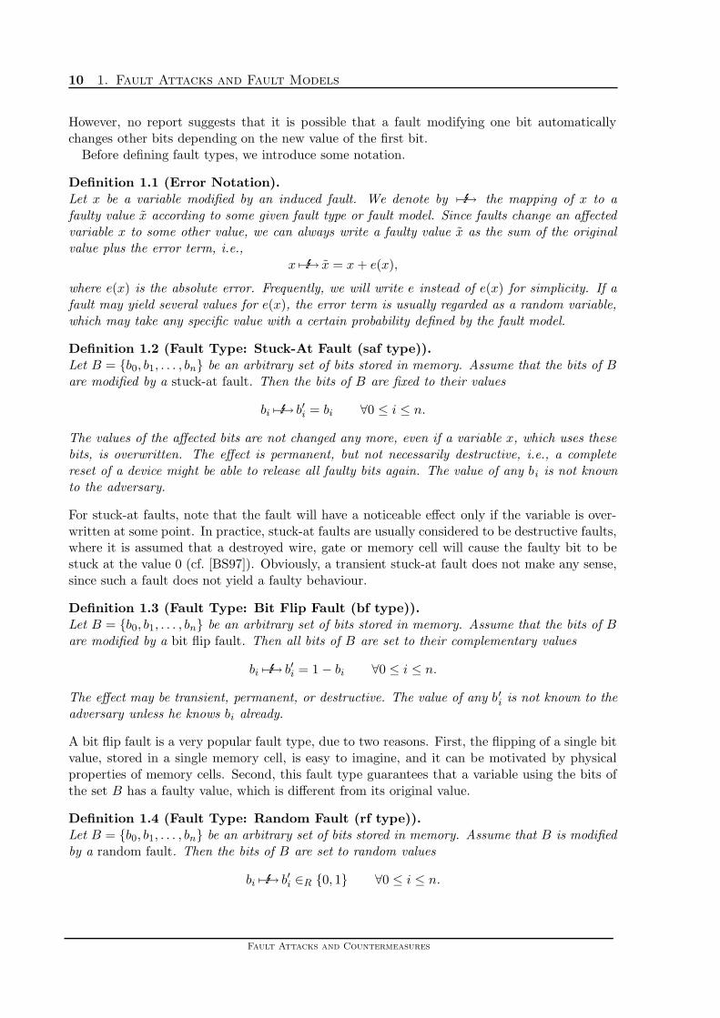
Before defining fault types, we introduce some notation.
Definition 1.1 (Error Notation).Let x be a variable modified by an induced fault. We denote by 7−→E the mapping of x to afaulty value x according to some given fault type or fault model. Since faults change an affectedvariable x to some other value, we can always write a faulty value x as the sum of the originalvalue plus the error term, i.e.,
x 7−→E x = x + e(x),
where e(x) is the absolute error. Frequently, we will write e instead of e(x) for simplicity. If afault may yield several values for e(x), the error term is usually regarded as a random variable,which may take any specific value with a certain probability defined by the fault model.
Definition 1.2 (Fault Type: Stuck-At Fault (saf type)).Let B = {b0, b1, . . . , bn} be an arbitrary set of bits stored in memory. Assume that the bits of Bare modified by a stuck-at fault. Then the bits of B are fixed to their values
bi 7−→E b′i = bi ∀0 ≤ i ≤ n.
The values of the affected bits are not changed any more, even if a variable x, which uses thesebits, is overwritten. The effect is permanent, but not necessarily destructive, i.e., a completereset of a device might be able to release all faulty bits again. The value of any bi is not knownto the adversary.
For stuck-at faults, note that the fault will have a noticeable effect only if the variable is over-written at some point. In practice, stuck-at faults are usually considered to be destructive faults,where it is assumed that a destroyed wire, gate or memory cell will cause the faulty bit to bestuck at the value 0 (cf. [BS97]). Obviously, a transient stuck-at fault does not make any sense,since such a fault does not yield a faulty behaviour.
Definition 1.3 (Fault Type: Bit Flip Fault (bf type)).Let B = {b0, b1, . . . , bn} be an arbitrary set of bits stored in memory. Assume that the bits of Bare modified by a bit flip fault. Then all bits of B are set to their complementary values
bi 7−→E b′i = 1 − bi ∀0 ≤ i ≤ n.
The effect may be transient, permanent, or destructive. The value of any b′i is not known to theadversary unless he knows bi already.
A bit flip fault is a very popular fault type, due to two reasons. First, the flipping of a single bitvalue, stored in a single memory cell, is easy to imagine, and it can be motivated by physicalproperties of memory cells. Second, this fault type guarantees that a variable using the bits ofthe set B has a faulty value, which is different from its original value.
Definition 1.4 (Fault Type: Random Fault (rf type)).Let B = {b0, b1, . . . , bn} be an arbitrary set of bits stored in memory. Assume that B is modifiedby a random fault. Then the bits of B are set to random values
bi 7−→E b′i ∈R {0, 1} ∀0 ≤ i ≤ n.
Fault Attacks and Countermeasures

1.3: Definition of Fault Types 11
The random choices of all b′i are assumed to be independent. Unless otherwise noted, the uniformdistribution is assumed. The effect may be transient, permanent, or destructive. Again, the valueof any b′i is not known to the adversary.
A random fault is usually considered to be the most realistic fault type. Since several physicalmethods of fault induction are hard to control precisely, non-destructive physical stress is mostlikely to change a variable according to the random fault type. Beyond that, some authors haveeven called stuck-at faults and bit flip faults controversial (e.g., [YKLM01a]).
Usually, a random fault is assumed to create a bit value b′i = 0 with probability 1/2 and b′i = 1with probability 1/2. However, some authors have also considered an asymmetric distribution,where it is much more likely that a bit is reset to 0 rather than set to 1. This has been usedfor attacks on unknown symmetric cryptosystems in [BS97], and it has been mentioned, butnot used, in [BDL97]. Such asymmetric distributions are usually motivated by specific physicalattacks. It could be reasoned that faults, which always (or almost always) cause bits to be setto 0 should be considered as an additional fault type. However, this has not been done beforein the literature and such faults have been considered only once, in [BS97]. Hence, we stick totradition and do not define this as a new fault type.
Similarities and Differences Between Fault Types. The above three fault types, (saf), (bf)and (rf) fault types, have already been described in the earliest publications concerning faults,[AK96] and [AK97], and they have been used in many publications since then.
Although the three fault types are fundamentally different, these differences are usually notaddressed in publications. The reason for this is the fact that in practical attacks, it is sufficientthat a certain effect occurs at some time. For example, an attack assuming the bit flip faulttype will usually also be successful if the random fault type is used instead.
The reason that most of the times, one fault type can be replaced by another fault type, isthat attacks usually only require that a specific effect occurs at some time. If an adversary cansomehow detect if a desired effect occurs or not, he does not have to use a specific fault type. Itis usually acceptable if an adversary has to induce faults multiple times during an attack until adesired effect occurs. For example, both stuck-at faults and bit flip faults can be interpreted asrandom faults with extreme distributions, which depend on the actual value of any individualbit. Hence, the effects of stuck-at faults or bit flip faults can also be achieved given the randomfault type and enough attempts. On the other hand, a uniformly distributed random fault canbe seen as a bit flip fault with a success probability of only 1/2 for every affected bit.
Given the random fault type, all bits from the targeted set B might be changed to the valuesthey already had. If the duration of the fault is transient, the attack will not be noticeable.This also holds for individual bits, e.g., given a bit bi, no error will be detected in bit bi, if thefault results in b′i = bi. However, if b′i 6= bi, the effect is the same as for the bit flip fault type.Hence, it is possible to interpret a fault affecting a set B of n bits using the random fault typeas a fault affecting only a subset B ′ ⊆ B using the bit flip fault type. Here, B ′ contains all thosebits from B, whose values have been changed.
For simplicity, most authors assume only bit flips if the attack assumes single faulty bits. Formultiple faulty bits, the random fault type is usually preferred. To our knowledge, stuck-atfaults have only been used in [BS97] as destructive faults. We are also not aware of any attackwhich explicitly uses the fact that a bit flip fault is guaranteed to change a fixed set of multiplebits to their complementary value. Most attacks described in the open literature, which rely onclassical fault types, work for any of these three types.
Martin Otto, Dissertation, December 2004

12 1. Fault Attacks and Fault Models
The next fault type is based on experiments described in [SA02] and [QS02]. They have beendescribed in detail in Section 1.1. The name of this fault type is due to [BS03].
Definition 1.5 (Fault Type: Bit Set Or Reset Fault (bsr type)).Let B = {b0, b1, . . . , bn} be an arbitrary set of bits stored in memory. Assume that B is modifiedby a bit set or reset fault. Then the bits of B are set to chosen values
bi 7−→E b′i = ci, ci ∈ {0, 1} ∀0 ≤ i ≤ n.
The important fact about this fault type is that the values ci are known and are usually chosenby the adversary. The effect may be transient, permanent, or destructive. The original valuesof the bits of B are not known to the adversary.
Definition 1.5 shows that the effect of the random fault type can be realized using the bit set orreset fault type, but the effects of both the stuck-at fault type and bit flip fault type can onlybe realized if the original values of the bits are known. However, since the adversary can choosethe values ci freely, he can choose them uniformly i.i.d. (independent identically distributed) atrandom and can thus achieve the effect of a stuck-at fault or a bit flip fault with a probabilityof 1/2n+1.
The bit set or reset fault type, however, is fundamentally different from the other three faulttypes, since an adversary can set any specific bit to any chosen value. This represents anextremely powerful adversary. It is the strongest fault type known and modern smartcards takeseveral measures to reduce the power of such an adversary. Taking the properties of modernsmartcards into account, this fault type may be assumed as almost impossible to achieve inpractice.
1.4. Definition of Fault Models
Since characterizing fault attacks requires more than just the specification of the fault type,we will now describe a variety of fault models, which yield complete descriptions of fault attacksettings. We will present the most popular fault models, which have been used extensively in theliterature, and we will derive new justifications for known fault models by carefully examiningthe properties of modern high-end smartcards and the power of an up-to-date adversary. As wehave explained before, fault models need to be justified by possible real world attacks in orderto be considered as valid. Therefore, we will always present both a motivation from the realworld for our fault models, as well as a brief overview over the literature, showing where thesefault models have been used.
Modern Smartcards. To derive reasonable fault models, which can be justified by physicalattacks, we combine parameter settings known from actual attacks with hardware countermea-sures in effect on the card. Since this thesis approaches fault attacks from an algorithmic pointof view, we do not go into depth when describing the physical properties and the details on chipcard and integrated circuit design, neither do we describe hardware countermeasures in detail.We refer the interested reader to [RE00] for details. As a reasonable sketch for the architectureof modern high-end smartcards, we present Figure 1.2.Since we are guided by practical considerations, we always assume the most powerful adversary,i.e., the adversary presented and justified by experiments in [SA02] and [QS02]. This adversaryis able to use the bit set and reset fault type defined in Definition 1.5, which yields an extremely
Fault Attacks and Countermeasures

1.4: Definition of Fault Models 13
RSA acceleratorBEU
RNGrandom number generator
CPUBEU bus encryption unit
AS address scrambler
EEPROM ROM RAMprivate user keys
OS, RSA, COMP128,system keys
Figure 1.2.: Architectural sketch of a modern high-end smartcard.
strong adversary. Such an adversary can target any specific area on the card at a precise time(on his clock) and set the stored bit to any specific value. We also consider smartcards withseveral hardware countermeasures in effect (see [RE00], [KK99]). In these realistic scenarios, theeffective power of the adversary is reduced significantly, e.g., knowledge about the location of theinduced fault does not need to imply knowledge about the position of the bit within an algorithm.Similarly, precise timing not necessarily implies knowledge of the actual step performed at thattime. There are three most important hardware countermeasures used on modern smartcards.First, a randomized clock is used to blur the timing behaviour of a device. Second, memory anddata encryption is incorporated to ensure that a large number of bits is affected if a single bitis flipped by a fault. Third, address and bus line scrambling is employed such that the physicallayout of the memory cells does not reflect the logical layout. These countermeasures degradethe power of the strongest adversary known today. In the discussion of the fault models definedbelow, we will give examples of how the adversary is weakened. In general, the stronger thecountermeasures of a smartcard, the weaker the attack and the more bits are affected by anattack. The following fault models can be motivated by gradually improving the strength of thecard’s countermeasures.
The resulting fault models describe faults induced into a single bit, into a bounded numberof bits, e.g., a byte, and into all bits of a given variable. Some fault attacks just require theinduction of an unspecified fault, such as the attack on CRT-RSA described in Chapter 3. Andlast, some attacks only require the knowledge whether a fault occurred or not.
Throughout this thesis, we will always assume that an adversary can only induce a single faultduring each run of an attacked algorithm. This implies that only one variable may be targeted.This is an important restriction, used throughout the literature. It ensures that an adversarycannot induce faults into both, a certain variable and a checking procedure. Otherwise, hecould try to make sure that internal checks are circumvented. Although some authors suggestthat no checking procedure should represent a single point of failure (cf. [AK96], [YKLM01b]),there have been no reports anywhere suggesting that such correlated attacks are possible with areasonable success probability. Only once, multiple, yet uncorrelated faults have been considered(in [BS97]). However, this has not led to a new type of attacks. Besides that, it should be clear
Martin Otto, Dissertation, December 2004

14 1. Fault Attacks and Fault Models
that during a fault attack, an adversary may run the attacked device multiple times, and mayinduce faults during each execution.
We also assume that an adversary cannot change the fault model during an attack. Thisrestriction is motivated by the assumption that an adversary uses only a single means of physicalattack to induce faults. This is a reasonable assumption, as otherwise, we could just define anew fault model, capable of catching all aspects of a given attack with multiple different effects.However, such an attack has not yet been described anywhere in the literature.
1.4.1. Fault Models Affecting a Single Bit
In this section, we describe fault models, where faults affect only a single bit of a targetedvariable. Such scenarios assume a very strong adversary and it has been claimed by someauthors that such fault models are unrealistic in practice (cf. [YKLM01a], [Dot02]). Since alltrustworthy smartcards are fully armed with a variety of countermeasures, precise control of thelocation of an affected bit or byte seems to be unrealistic these days. However, fault modelsassuming a single faulty bit, usually based on the bit flip fault type, are very popular faultmodels, which are widely used for fault attacks.
Chosen Bit Fault Model
We first describe the strongest adversary, which can be justified by experiments today. Here,the bit set or reset fault type from Definition 1.5 is assumed for an adversary, who attacks anunprotected card.
Definition 1.6 (Fault Model: Chosen Bit Fault Model).We define the Chosen Bit Fault Model with the following parameters.
location: complete control (a specific bit of a specific variable used in a specific lineof code of an attacked algorithm can be targeted)
timing: precise control (can target a specific point of time, if the affected variableis used in a loop, a specific iteration can be targeted)
number of bits: one bit of the affected variable is changedfault type: bit set or reset faults (as defined in Definition 1.5)probability: certain (every physical attack results in a fault of the desired kind, but if
the adversary sets the targeted bit to its original value, the correct resultwill be returned)
duration: permanent faults and transient faults (both variants are investigated if theydiffer, however, it is assumed that an adversary cannot use both kindsduring one fault attack)
Mathematical model: The effect of an attack using this fault model on a targeted variable canbe modeled as an addition or subtraction of a single bit, i.e., a variable X is changed to
X 7−→E X = X ± 2k for 0 ≤ k ≤ l(X) − 1.
Both k and the sign of ±2k are assumed to be chosen by the adversary.
Motivation from the Real World. The Chosen Bit Fault Model resembles the (bsr) fault typethat is achieved by physical attacks described in [SA02] or [QS02]. It can be achieved by inducing
Fault Attacks and Countermeasures

1.4: Definition of Fault Models 15
faults into RAM or EEPROM of an unprotected smartcard. Although high-end smartcardsimplement sophisticated hardware countermeasures, many smartcards currently used are eithertoo old or too cheap to do so. Hence, this fault model is a realistic one for such cards. It assumesthe strongest adversary and the weakest card.
Although this model is unrealistic for modern high-end smartcards, it is a particularly inter-esting model, since algorithms secure in this fault model are secure in the weaker models aswell.
Motivation from the Literature. The Chosen Bit Fault Model has been considered in [Dot02]for attacks on FLASH, SFLASH and QUARTZ, but has not been worked out since the modelhas been considered “not to be very realistic”. It has also been considered briefly in [BS97]. Wehave proposed this fault model as “Fault Model #1” in [BOS03].
Single Bit Fault Model
We now describe the most important and mostly used fault model, the fault model introducedby Boneh, DeMillo, and Lipton in the first paper about fault attacks, [BDL97].
Definition 1.7 (Fault Model: Single Bit Fault Model).We define the Single Bit Fault Model (or BDL Fault Model) with the following parameters.
location: loose control (a specific variable used in a specific line of code of an attackedalgorithm can be targeted, but no specific bit of the variable can be targeted)
timing: no control (cannot target a specific point of time, if the affected variable isused in a loop, every iteration of that loop is hit with the same (uniform)probability)
number of bits: one bit of the affected variable is flipped (every bit of the variable is hitwith the same (uniform) probability)
fault type: bit flip faults (as defined in Definition 1.3)probability: certain (every physical attack results in a fault of the desired kind)duration: permanent faults and transient faults (both variants are investigated if they
differ, however, it is assumed that an adversary cannot use both kindsduring one fault attack)
Mathematical model: The effect of an attack using this fault model on a targeted variable canbe modeled as an addition or subtraction of a single bit, i.e., a variable X is changed to
X 7−→E X = X ± 2k for 0 ≤ k ≤ l(X) − 1.
The bit position k is assumed to be chosen according to the uniform distribution and subsequentchoices are assumed to be i.i.d..
Fault Model 1.7 could be further relaxed, to use random faults instead of bit flip faults as thefault type. Since only a single bit is affected, a uniformly distributed random fault has thesame effect as a bit flip fault with success probability 1/2. Although being more realistic, thisrelaxation does not yield new attacks. Using the bit flip fault type simply means to neglect allfaults, which change a bit to the original value. This is a reasonable approach since such faultsdo not yield a faulty result. Therefore, it is not necessary to assume random faults. Originally,
Martin Otto, Dissertation, December 2004

16 1. Fault Attacks and Fault Models
it is noted in [BDL97] that the authors assume a physical setup, where the induced faults aremore likely to flip bits from 1 to 0, rather than from 0 to 1. However, they do not use suchan asymmetric behavior and do not consider it in their fault model. Therefore, we neglect thisproperty as well and assume a uniform distribution of bit flips.
The mathematical model of Fault Model 1.7 also neglects the fact, that bit flips can only flipthe current value of a bit in reality, i.e., only one of the two possible error terms +2k or −2k isactually possible. However, the chosen model simplifies notation and analysis. Moreover, it isthe standard model used in the literature. Therefore, we use this mathematical model as well.
Motivation from the Real World. The Single Bit Fault Model is unrealistic for modern high-end smartcards, which are armed with a variety of countermeasures. Such a protection preventsan adversary from realizing the bit set or reset fault type. However, there are cards, which aretoo old or too cheap to incorporate sufficient countermeasures. If a card at least uses addressscrambling for every single variable or bus line scrambling, the adversary’s power is degraded toFault Model 1.7. The main motivation for this model, however, comes from literature. Here, itis very popular, since it is an easy model, which allows to describe fault attacks in a simplifiedsetting, which can then be generalized to a larger number of affected bits.
Motivation from the Literature. Fault Model 1.7 is one of the oldest and most prominentfault models. It has been used explicitly in [BDL97] and [BDL01] for attacks on plain RSA.It has also been used for fault attacks among others in [BS97] (where it is also considered ina relaxed version, where the targeted variable is unknown), and in [JQ97a], [JQ97b], [Pet97],[BDH+98], [BMM00], [YKLM01b], [Dot02], [JQYY02], [JBF02], [YKLM03], [GA03], [CJ03],and [BCN+04].
1.4.2. Fault Models Affecting a Bounded Number of Bits
Another common model assumes that only a bounded number of bits (“multiple bits”, “fewfaulty bits”) are affected by an induced fault. This model catches the fact that mobile devicesstore and load variables in blocks, where the length of a block is the word size of a device. Theword size is usually one byte, hence, attacks which assume that a byte is affected by inducedfaults are considered to be the most realistic fault attacks in several papers (e.g., [PQ03], [GK04]).Hence, if the standard block size on smartcards increases, the fault model defined below shouldbe adapted to that change. A bounded number of bits may also be affected by faults, whichtarget a specific bit, but have such a strong effect on the memory that neighbored bits arechanged as well. In this case, the fault is smeared over a bounded number of surrounding bits,where boundary bits are possibly changed with a lower probability than the target bit. However,it is more practical to assume a random change of the whole byte. Moreover, we are not awareof any attack, which exploits a probability distribution other than the uniform distribution.
The byte fault model represents all attacks, where an unspecified “small” number or “multiple”bits are affected by the induced faults. In all such cases, the number of attacked bits is assumedto be small enough such that all possible error patterns are efficiently sampleable. This allows anadversary, who does not know how the faulty bits have actually been changed, to try all possiblepatterns as a basis for a recovery of secret data. The goal of such an exhaustive enumeration isto identify the correct error pattern. An exhaustive search requires that the number of faultybits can be bounded by a small number. Therefore, many authors, who assume “multiple” faulty
Fault Attacks and Countermeasures

1.4: Definition of Fault Models 17
bits, assume some variant of the byte fault model, which may in some cases cover few more thanjust 8 bits.
Definition 1.8 (Fault Model: Byte Fault Model).We define the Byte Fault Model with the following parameters.
location: loose control (a specific variable used in a specific line of code of an attackedalgorithm can be targeted, but no specific block of 8 bits of the variable canbe targeted)
timing: no control (cannot target a specific point of time, if the affected variable isused in a loop, every iteration of that loop is hit with the same (uniform)probability)
number of bits: few faulty bits, i.e., one byte (8 bits) of the affected variable is changed(every block of 8 bits of the variable is hit with the same (uniform) proba-bility)
fault type: random faults (as defined in Definition 1.4)probability: certain (every physical attack results in a fault of the desired kind, but with
probability 1/256 all affected bits are set to their original value and thecorrect result is returned)
duration: permanent faults and transient faults (both variants are investigated if theydiffer, however, it is assumed that an adversary cannot use both kinds inone attack setting)
Mathematical Model: The effect of an attack using this fault model on a targeted variable canbe modeled as an addition or subtraction of an unknown error byte at an unknown position, i.e.,an affected variable X is changed to
X 7−→E X = X ± b · 2k for an unknown 0 ≤ k ≤ l(X) − 8 and an unknown b ∈R Z28 .
In this model, we assume that both b and k are chosen i.i.d. at random from the correspondingsets of possible values according to the uniform distribution.
Usually, a device will load and store parameters in fixed blocks of 8 bits, starting with the leastor most significant byte. Therefore, in practice, not all sets of 8 contiguous bits may be equallylikely to be affected by a byte fault. However, this aspect is usually neglected, as long as it isnot important for the analysis which byte is faulty. It simplifies analysis at a negligible cost.Hence, we assume that any block of 8 contiguous bits is hit with the same uniform probability.
In the case of transient faults, one can simply consider all those bits to be faulty, whose valueshave been flipped by the random fault type. This allows to exchange the fault type in FaultModel 1.8 to the bit flip fault type. This interpretation is used by many authors, who simplyassume “multiple” faulty bits.
A popular way to relax the Byte Fault Model is to allow that the affected bits are notcontiguous, which is done by several authors, who assume “multiple” faulty bits. For a variableof length n, there are less than n8 possible sets of 8 different bits, hence, from a complexitytheoretic point of view, testing all these possible sets adds only a polynomial factor to theoverall complexity. This remains true as long as the number of affected bits is a constant, whichguarantees that the number of tests is small enough.
Martin Otto, Dissertation, December 2004

18 1. Fault Attacks and Fault Models
Motivation from the Real World. In the real world of modern high-end smartcards, this modelis motivated in three variants.
The Byte Fault Model as defined above is motivated by an adversary, who is able to inducebit set or reset faults, and a smartcard, which uses block-wise memory encryption or bus lineencryption and address scrambling on RAM and EEPROM (cf. [RE00]). Usually, all data storedin EEPROM and RAM is encrypted ([RE00]). Hence, if a fault is induced into memory, the valueof the affected block seen by the CPU will be unpredictable. Therefore, encryption degradesthe power of the adversary, since any single modified bit in memory affects a whole byte ofdata. Address scrambling prevents the attacker to specify when the faulty block is requested bythe CPU. However, we assume that the memory layout allows an adversary to target a specificvariable. The same model is derived if the bus lines are targeted. We have proposed this faultmodel before as “Fault Model #3” in [BOS03].
As a second variant of the Byte Fault Model, we may assume that the adversary knows whichbyte of the targeted variable is faulty. In the mathematical model, this can be expressed bya known parameter k. This model is motivated in the real world by the fact that the strongadversary’s power is reduced on smartcards if only encryption of the data is used and no addressscrambling. We have proposed this fault model as “Fault Model #2” in [BOS03].
As a third variant of Fault Model 1.8, a generalized version may be assumed, where theadversary knows that only one byte is changed, but he has no control on both timing andlocation. In this case, he might not know which variable was affected by his attack. In themathematical model, this can be expressed by assuming that the variable X is randomly chosenfrom a set of possible variables. In the real world, this variant can be motivated by two scenarios.First, a smartcard could use block-wise memory encryption and address scrambling as above.However, we now assume that the memory layout does not allow an adversary to target aspecific variable. Second, a smartcard may use memory encryption in RAM and EEPROMtogether with a randomized clock (cf. [CCD00]). In this case, the strong adversary’s power iseffectively reduced to this model. Memory encryption causes any single bit fault to affect a wholeblock of data. In this case, the attacker knows that a successfully induced fault will change ablock of data. However, the randomized clock implies that he does not know the exact time ofthe change within the algorithm. If he targets intermediate variables in RAM, in an accelerator,in cache memory, or the bus lines, the attacker does not know the position of the block as it isused in the CPU. We have proposed this fault model as “Fault Model #3’ ” in [BOS03].
Motivation from the Literature. Variants of the byte fault model as defined above have beenused in [BDL01] (where “a small number of bits flips” are assumed), in [JQ97b] (where “multiple”faulty bits and bit flips are assumed), in [BDH+98] (where multiple faulty bits are assumed,whose positions are known), in [JQYY02], in [PQ03] (who also consider a relaxed model wherethe affected variable is not exactly known), in [GA03] (where “a few” bits are assumed to befaulty, e.g., 6), in [BCN+04] (where multiple bits do not need to be contiguous), in [GK04] (whoquote our “Fault Model #3” from [BOS03]), and in [Wag04] (where only l(x)/8 possible bytes ina variable x are considered). Additionally, it is mentioned in [YJ00], and in [YKLM01a] (wherea “limited number of faulty bits” is referred to as more difficult to achieve than an arbitrarynumber of faulty bits). In [Wag04], the author also proposed an extreme version of a boundedfault model, where all but the 160 most significant bits of a 1024 bit RSA modulus are affected.However, this model has not been motivated by real world considerations.
Fault Attacks and Countermeasures

1.4: Definition of Fault Models 19
1.4.3. Fault Models Affecting an Arbitrary Number of Bits
Random Fault Model
Sometimes, an adversary knows not enough about his induced faults to bound their effectssufficiently. While he knows the affected variable, he does not know how the change of a singlebit affects the value of the variable. In this case, it is sometimes reasonable to assume that anaffected variable is changed to some random value. As long as all values might occur with non-negligible probability, using the assumption that the resulting values are distributed uniformlyis a reasonable simplification for analyses.
Definition 1.9 (Fault Model: Random Fault Model).We define the Random Fault Model with the following parameters.
location: loose control (a specific intermediate variable used in an attacked Algorithmcan be targeted)
timing: no control (cannot target a specific point of time, every line of code / everyiteration of a loop, is hit with the same (uniform) probability)
number of bits: random number of bits, i.e., all bits of the targeted variable are affected, thevalue is replaced with a random value in situ, i.e., using the same numberof bits, leading zeros allowed (all possible random values occur with thesame (uniform) probability)
fault type: random faults (as defined in Definition 1.4)probability: certain (every physical attack results in a fault of the desired kind, but the
original value is allowed to appear as well)duration: transient and permanent faults (both variants are investigated if they differ,
however, it is assumed that an adversary cannot use both kinds during onefault attack)
Mathematical Model: The effect of an attack using this fault model on a targeted variable canbe modeled as an addition or subtraction of an unknown error from a bounded set. We assumethat a targeted variable X is changed to some random value, i.e., X ∈ [0, 2l − 1]. In this model,a fault may result in any faulty value. We have
X 7−→E X = X + e(X) with e(X) ∈R {−X,−X + 1, . . . , 2l − X − 1}.Here, l is the maximal length the variable X may take. If X ∈ Zp, we have l = l(p − 1) =blog2(p − 1)c + 1. Otherwise, l is the maximal length of the memory space reserved for X. Weassume that the random variable e(X) takes any value from the set {−X,−X + 1, . . . , 2l −X −1} with the same (uniform) probability and that subsequent choices are i.i.d. according to theuniform distribution.
The Random Fault Model can be used if an adversary either knows that an induced fault will setthe affected variable to a random value according to the uniform distribution, or if the successof his fault attack does not rely on special values to appear at some time or with a specificprobability. The naming of this fault model should not be confused with the random fault typefrom Definition 1.4, however, the intuition behind both concepts is similar, both describe thata given set of bits is replaced by random bit values.
In practice, the adversary may be able to target a desired variable in a reasonable smallinterval of operations or even loop iterations. This interval may have been derived from other
Martin Otto, Dissertation, December 2004

20 1. Fault Attacks and Fault Models
sources of information, for example from the power profile of the card (see [ABF+02]). In thiscase, an adversary may gain some control on timing and bound the lines of codes or the loopiterations, in which the targeted variable has been hit.
As a more general variant of this fault model, one might also assume that even the affectedvariable is not known with certainty, e.g., an adversary might only be able to hit a variable froma set of a few different variables.
Motivation from the Real World. This scenario is motivated by strong high-end smartcardscompletely armed with countermeasures. Memory encryption, address scrambling and a ran-domized clock imply that any fault induced into memory or the CPU at a vague point will leavethe attacker at most with the information that a certain variable is faulty. It therefore enforcesa very weak adversary.
Motivation from the Literature. The Random Fault Model has been used for successful faultattacks in [YKLM01b], [Dot02] (for an attack on ESIGN-D), in [YKLM03], in [KKT04] (wherealso a different model was used which assumed that bits could only be set to 0), and in [PV04].We have proposed this fault model as “Fault Model #4” in [BOS03].
Arbitrary Fault Model
We now describe the weakest fault model. Here, an adversary can only target a specific line ofcode or a set of several intermediate variables. He does not have any additional information,e.g., about the type of the fault or the error distribution. Attacks based on this weak adversaryare extremely dangerous, because the weaker an adversary, the more practical the attack.
Definition 1.10 (Fault Model: Arbitrary Fault Model).We define the Arbitrary Fault Model with the following parameters.
location: loose control (a specific line of code can be targeted, but no specific variableused in that line)
timing: no control (cannot target a specific point of time, if the affected line of codeis from a loop, every iteration of that loop is hit with the same (uniform)probability)
number of bits: random number of faulty bits (any number of bits may be affected using anunknown probability distribution, however, at least one bit is changed)
fault type: unknown (any fault type is possible, but the adversary does not know thetype)
probability: certain (every physical attack results in a fault of the desired kind, i.e.,the final result computed by the affected line of code is different from thecorrect result)
duration: transient and permanent faults (both variants are investigated if they differ,however, it is assumed that an adversary cannot use both kinds during onefault attack)
Mathematical Model: The effect of an attack using this fault model on a targeted line of codecan be modeled as an addition or subtraction of an unknown error from a bounded set. Let Xbe the variable, which is assigned the result of the affected line of code. Then in the Arbitrary
Fault Attacks and Countermeasures

1.4: Definition of Fault Models 21
Fault Model, X is changed to the faulty value X, such that
X 7−→E X = X + e(X) with e(X) ∈R {−X,−X + 1, . . . , 2l − X − 1} \ {0}.
Here, l is the maximal length the variable X may take. If X ∈ Zp, we have l = l(p − 1) =blog2(p − 1)c + 1. Otherwise, l is the maximal length of the memory space reserved for X. Weemphasize the fact that the probability distribution of the random variable e(X) is arbitrary andunknown.
In some situations, an adversary has extremely limited control over the induced faults. He maytarget a specific line of code, but it is unknown, which variable is affected and how that variableis changed. Since the Arbitrary Fault Model assumes very little information about the fault, allother fault models defined above can be used for attacks based on the Arbitrary Fault Model.
The Arbitrary Fault Model is not equivalent to the Random Fault Model 1.9. Basically,we have two differences. First, the Random Fault Model allows an adversary to assume thatany specific error value appears with some known probability. This is not the case for theArbitrary Fault Model, where the probability distribution is completely unknown. Second, anadversary using the Random Fault Model can target any specific variable, while the ArbitraryFault Model only allows to target a specific line of code. This implies that in the Arbitrary FaultModel, transient faults on any variable or operation used in an affected line of code yield thesame situation as if the result of the targeted line of code had been changed by the fault. Forpermanent faults however, the affected variable is not known with certainty. In this case, it isusually assumed that any variable used in the targeted line of code is hit with the same uniformprobability. Hence, if an attack depends on a specific variable being affected, this situation willoccur among a known (low) number of induced faults. This information is usually sufficient forfault attacks.
A fault attack, whose setting is described by the Arbitrary Fault Model, can be successful, ifthe adversary does not need to be able to guess the error term in order to derive information,and if he does not need assumptions about the distribution of the error value. He must be ableto recover the secret data with any non-zero error value. Usually, an adversary cannot checkall possible error values, since the set of possible bit patterns is not assumed to be efficientlysampleable in this model.
A generalized version may assume that an adversary cannot target a specific line, but will hitany line with a known probability, e.g., according to the uniform distribution. In this case, oneout of several attacks can be expected to hit a desired line. This may be sufficient for success.
Motivation from the Real World. The Arbitrary Fault Model assumes the weakest adversary.In practice, the strong adversary’s power of inducing bit set or reset faults may be reduced tothis model in the presence of a large variety of countermeasures. Modern high-end smartcardsfeature a great variety of sensors and filters, hence, inducing faults is not an easy task. However,it is not impossible to do so. Still, the adversary may not be able to bound the effect of aninduced fault sufficiently to assume other, stronger fault models.
Motivation from the Literature. This fault model has been used for fault attacks on CRT-RSA in [BDL97] and [BDL01]. This attack is discussed in detail in Chapter 3. Here, any fault,which changes the final result of a certain line of code, is sufficient to recover the secret key.This fault model has also been used in [JKQ97], [ABF+02], and [YMH03].
Martin Otto, Dissertation, December 2004

22 1. Fault Attacks and Fault Models
1.5. Validity and Applicability of the Proposed Fault Models
The five fault models presented in the last sections have been motivated by a real world scenario,comparing the power of the adversary with the power of the countermeasures present on asmartcard. This has been described in detail in the paragraphs titled “motivations from thereal world”. We always assume the strongest adversary known from open literature, i.e., anadversary capable of using the bit set and reset fault type from Definition 1.5. Depending onthe strength of the smartcard’s countermeasures, this power is weakened.
The Chosen Bit Fault Model is the strongest fault model possible. An adversary who is ableto apply a Chosen Bit Fault Model can recover any bit of any variable used in an algorithm.This can be done by an oracle attack (which will be discussed in Section 1.6.2). However, thisfault model is extremely unrealistic for modern smartcards, since smartcard manufacturers areaware of the danger of fault attacks. However, it might still be valid for old or cheap smartcards.Moreover, it is a particularly interesting model, since algorithms secure in this fault model aresecure in the weaker models as well.
The Single Bit Fault Model assumes some protection of the smartcard, however, sensitivecryptographic applications will not be implemented on such cards anymore. However, due to itssimple modeling, it is a very popular starting point to analyze the security of algorithms againstfault attacks.
The Byte Fault Model represents a moderately strong adversary. It assumes a fairly wellprotected smartcard. Hence, it is much more realistic than the fault models assuming a singlefaulty bit, but it is not clear, to what extent smartcards are being manufactured, which allowthis model. It is definitely unrealistic for modern high-end smartcards. Just like the previous twofault models, it may still be valid for old or cheap smartcards. Moreover, if the best protectedcards should exhibit vulnerabilities in their line of defense, an adversary will most probable beable to base his attacks on this fault model. Therefore, it does have practical relevance.
The best protected smartcards degrade any powerful adversary known today to the RandomFault Model or even the Arbitrary Fault Model.
The Random Fault Model is one of the most realistic fault models to assume. Modern high-end smartcards will ensure that an adversary cannot hope to base successful attacks on anyof the stronger fault models. Therefore, algorithmic countermeasures which aim at defendingdevices against attacks based on this fault model are needed.
The Arbitrary Fault Model is the most realistic fault model assuming the weakest adversary.It is a very practical model, since it can be realized by any physical attack, which can be mountedwith a sufficiently high success probability. Attacks, which are successful in the Arbitrary FaultModel are also successful in any other fault model. However, the Arbitrary Fault Model is onlyrealistic for a modern, high-end, and expensive smartcard.
We present a comprehensive summary of the defined fault models in Table 1.7.
A smartcard may react in various ways to an induced fault: Unprotected cards will fail tonotice the fault and output a faulty result, leaving them vulnerable to a successful fault attack.Well protected cards may detect some or most induced faults by internal checking proceduresand react with some error behaviour, e.g., with an error message or with a security reset.An error message may either depend on the actual error detected or may be unspecific. Theoptimal protected cards are equipped with a variety of additional hardware countermeasures (see[BS03]), which might detect some physical attacks even before the attack successfully inducesan error. In this case, a complete security reset is triggered. Such countermeasures are ideal,since they prevent faults before they occur. Unfortunately, countermeasures which are capable
Fault Attacks and Countermeasures

1.5: Validity and Applicability of the Proposed Fault Models 23
Chosen BitFault Model
Single BitFault Model
ByteFault Model
RandomFault Model
ArbitraryFault Model
Definition 1.6 1.7 1.8 1.9 1.10
control onlocation
complete loose loose loose loose/no
control ontiming
precise no no no no
number ofaffected bits
1 1 8 random random
fault type (bsr) (bf) (rf) (rf) unknown
successprobability certain in all models
duration all consider transient and permanent faults
Table 1.7.: Overview of the fault models defined in Section 1.4
of preventing any possible physical fault induction are unrealistic, especially given the factthat new physical attacks are reported frequently. This emphasizes the need for algorithmiccountermeasures and checking procedures, which do not depend on the physical attack, butonly on the induced fault.
Therefore, an adversary can always hope to apply some physical attack, which cannot beprevented by the attacked card. All the fault models presented in Section 1.4 represent changesof the data used by a card. These fault models are used for actual attacks, where it is assumedthat the faulty final result is returned by the smartcard. This faulty final result allows theadversary to compute secret data in whole or in parts, possibly requiring a correct result as well.Such attacks will be described for plain RSA (Chapter 2), CRT-RSA (Chapter 3), and ellipticcurve cryptosystems (Chapter 5).
A natural approach to defend against these attacks is to incorporate checking procedures,which aim to prevent that faulty outputs are returned. Modern sophisticated smartcards mayhave both hardware and software countermeasures which alter the final result to some randomvalue or use detection mechanisms that report an error to the user without revealing a faultyoutput. However, any such countermeasure will always leak the information that an inducedfault successfully changed the internal data. Surprisingly, there are attacks, which are capableof recovering secret data only based on this information. We will refer to these attacks as oracleattacks, and describe this kind of fault attacks in Section 1.6.2.
If an adversary can recover secret data using an oracle attack, his attack is extremely power-ful. An attacked device can only hide the information whether a fault occurred or not with asignificant loss in efficiency. Assume that during a computation of a signature, a fault occurred,such that the final result is incorrect. If the device does not detect this, an adversary can simplycompare the output with the correct result and gets the information that a fault occurred. If thedevice detects this error, it may either react with an error behaviour such as an error message ora security reset, or it may invoke the computation once again. Both reactions can be detected,either by looking at the output, or at the increased duration of the operation (timing attack).Therefore, even if a device implements a large variety of (efficient) countermeasures, such as
Martin Otto, Dissertation, December 2004

24 1. Fault Attacks and Fault Models
checking the final result before output, it may not be able to withhold the desired informationfrom the attacker.
Hiding this information requires that the behaviour of a device does not change even if a faultoccurred. This implies that both the duration of a computation as well as the final result mustbe independent from any error. Since we always assume that only a single fault can be induced,the device needs to compute the final result at least twice. This doubles the computation time,which is a significant loss in efficiency. Even doubled computations may not be enough to besecure against permanent faults.
However, as we will show in Section 1.6.2, most oracle attacks rely on extremely powerful faultmodels, hence, their applicability in practice is controversial. Although we will not consider thiskind of fault attacks in depth in this thesis, we present in Chapter 7 an oracle attack on RSAbased on a new fault type, which will be developed in Section 4.5.
1.6. Other Attack Scenarios
1.6.1. Code Change Attacks
All fault models presented in the previous sections assume that data is manipulated, such thatvariable values used in an algorithm can be pertubated. However, we have described the pos-sibility that certain physical scenarios might induce faults in the program counter of a CPUor ALU, e.g., power spikes and clock glitches as presented in Section 1.1. This might causecertain operations to be skipped, yielding a code skip attack, it might cause certain operationsto be executed multiple times, or it might cause a loop counter to decrease. The latter has beendescribed theoretically in [BS97] and [PV04], whose authors suggest to induce faults into theloop counter to reduce the rounds in DES or pairing based cryptosystems to values, which allowto break the systems.
However, code attacks are not considered by many authors. In this thesis, we will only considerfault attacks on memory values, therefore, we will not describe code attacks in detail.
1.6.2. Oracle Attacks
As explained above, an oracle attack is a fault attack capable of recovering secret data basedonly on the fact whether an error occurred or not. Although such fault attacks are hard torealize in practice, we will demonstrate their power in this section. First, oracle attacks areformalized in the following definition.
Definition 1.11 (Oracle Attacks).Any fault attack, which unveils secret information from a cryptographic device only based on (atmost) a correct result and the information whether an induced fault changed the behaviour ofa device, is called an oracle attack. The induced faults may be defined according to any faultmodel.
Typically, oracle attacks require a much stronger fault model than other types of fault attacks. Inthis section, we will briefly present the main flavors of such attacks. Oracle attacks usually exploitconditional statements. Examples for such attacks are attacks using an extremely powerfulfault model (cf. [AK97]), and the more realistic memory-safe errors (cf. [YJ00], [JQYY02],[YKLM03]), and computational-safe errors (cf. [YKLM01a]). We will briefly introduce theseattacks.
Fault Attacks and Countermeasures
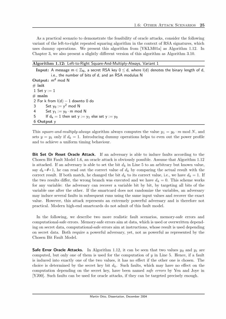
1.6: Other Attack Scenarios 25
As a practical scenario to demonstrate the feasibility of oracle attacks, consider the followingvariant of the left-to-right repeated squaring algorithm in the context of RSA signatures, whichuses dummy operations. We present this algorithm from [YKLM01a] as Algorithm 1.12. InChapter 3, we also present a slightly different version of this algorithm as Algorithm 3.10.
Algorithm 1.12: Left-to-Right Square-And-Multiply-Always, Variant 1
Input: A message m ∈ ZN, a secret RSA key 0 ≤ d, where l(d) denotes the binary length of d,i.e., the number of bits of d, and an RSA modulus N
Output: md mod N# init
1 Set y := 1# main2 For k from l(d) − 1 downto 0 do3 Set y0 := y2 mod N4 Set y1 := y0 · m mod N5 If dk = 1 then set y := y1 else set y := y0
6 Output y
This square-and-multiply-always algorithm always computes the value y1 = y0 · m mod N , andsets y = y1 only if dk = 1. Introducing dummy operations helps to even out the power profileand to achieve a uniform timing behaviour.
Bit Set Or Reset Oracle Attack. If an adversary is able to induce faults according to theChosen Bit Fault Model 1.6, an oracle attack is obviously possible. Assume that Algorithm 1.12is attacked. If an adversary is able to set the bit dk in Line 5 to an arbitrary but known value,say dk 7−→E 1, he can read out the correct value of dk by comparing the actual result with thecorrect result. If both match, he changed the bit dk to its correct value, i.e., we have dk = 1. Ifthe two results differ, the wrong branch was executed and we have dk = 0. This scheme worksfor any variable: the adversary can recover a variable bit by bit, by targeting all bits of thevariable one after the other. If the smartcard does not randomize the variables, an adversarymay induce several faults in subsequent runs using the same input values and recover the exactvalue. However, this attack represents an extremely powerful adversary and is therefore notpractical. Modern high-end smartcards do not admit of this fault model.
In the following, we describe two more realistic fault scenarios, memory-safe errors andcomputational-safe errors. Memory-safe errors aim at data, which is used or overwritten depend-ing on secret data, computational-safe errors aim at instructions, whose result is used dependingon secret data. Both require a powerful adversary, yet, not as powerful as represented by theChosen Bit Fault Model.
Safe Error Oracle Attacks. In Algorithm 1.12, it can be seen that two values y0 and y1 arecomputed, but only one of them is used for the computation of y in Line 5. Hence, if a faultis induced into exactly one of the two values, it has no effect if the other one is chosen. Thechoice is determined by the secret key bit dk. Such faults, which may have no effect on thecomputation depending on the secret key, have been named safe errors by Yen and Joye in[YJ00]. Such faults can be used for oracle attacks, if they can be targeted precisely enough.
Martin Otto, Dissertation, December 2004

26 1. Fault Attacks and Fault Models
Memory-Safe Errors. The authors of [YJ00] originally investigate the right-to-left repeatedsquaring algorithm in the context of RSA signatures (see Algorithm 2.3). However, the attackcarries over to Algorithm 1.12 seamlessly. The basis for an oracle attack is to induce a faultduring the computation of y1 = y0 ·m mod N in Line 4 of Algorithm 1.12. The authors assumethat the multiplication of y0 · m is interleaved with the modular reduction. To compute y0 ·m mod N , the variable y0 is scanned from left to right. If a fault is induced into memory cellsholding upper bits of y0 after these bits have been used by the computation, this fault hasno effect on the result y1. Hence, the value y1 is correct, while the value y0 is faulty. If thesecret key bit dk is 1, we have y = y1 and the faulty intermediate result y0 is overwritten, wheny0 = y2 mod N is computed in the next round. This implies that the faulty memory cells areoverwritten as well, and no error occurs. However, if dk = 0, the faulty value y0 is used in Line5 and y is faulty. It is assumed that if any intermediate variable y is faulty, the final resultof the algorithm will be faulty as well. This situation allows an oracle attack, since we havedk = 0 if and only if the final result is faulty and dk = 1 otherwise. The attack requires a strongadversary, who must be able to attack specific bits of y0 during a specific line of computationin a specific loop iteration. The attack becomes easier if the desired bits of y0 are stored inregister cells, which can be targeted by an adversary without changing the lower bits. Imprecisecontrol on location can be traded off for an increased number of attacks using statistics. Faultsas described above have been named memory-safe errors, because they occur in memory cells,which are no longer used in a computation, e.g., as in Line 4 of Algorithm 1.12.Memory-safe errors have also been described for oracle attacks in [JQYY02] and [YKLM03].
Computational-Safe Errors. The idea of memory-safe errors can be easily extended to interferewith the computation itself. While for memory-safe errors, some bits in memory are targeted,which are no longer used, computational-safe (or c-safe) faults aim at instructions, whose re-sult is no longer needed, so-called dummy instructions. In [YKLM01a], Yen et. al. describecomputational-safe errors.
The authors assume an attack on Algorithm 1.12. Here, the variable y1 is targeted. If a faultis induced during the computation of y1, the final result of Algorithm 1.12 is faulty if and onlyif we have dk = 1 and it is correct if dk = 0, since the value y1 is not used in this case. Whilestill representing a very strong adversary, the fault model assumed for computational-safe errorsis not as strong as for memory-safe errors. C-safe errors can be induced if an adversary is ableto target a specific instruction (during a specific iteration of a loop), however, since the effectof the induced fault in y1 is not important, control on location and timing does not need to beas precise as for memory-safe errors, where the upper bits have to be targeted after being used.Basically, an adversary has more time to attack y1 than to attack y0 without changing y1.
Contrary to the believe in [YKLM01a], the original (plain) repeated squaring algorithm canbe attacked by computational-safe errors as well (see Algorithms 2.2 and 2.3). Assume that afault is induced into the CPU of a device such that in the conditional statement, the executionof the then branch or the complete conditional statement is skipped. In this case, the final resultwill be wrong if dk = 1 and correct if dk = 0. Once again, the secret key bit can be recoveredusing the correct result, which is compared to the actual result to conclude whether the inducedfault yielded a faulty output or not. This attack requires that an adversary is able to haveinstructions skipped by the device, which is a very strong assumption. However, several authorsdescribe physical attacks, which potentially tamper with branch instructions, e.g., using powerspikes or clock glitches as presented in Section 1.1.
Additionally, any attack, which induces transient faults in intermediate variables used in a
Fault Attacks and Countermeasures

1.6: Other Attack Scenarios 27
dummy statement can potentially be a source for an attack using computational-safe faults. InAlgorithm 1.12, the value y0 is used in Line 4 and in Line 5. If a transient fault is induced intoy0 in Line 4, only the result y1 is faulty, the value y0 in Line 5 is set back to its original correctvalue. This also represents a computational-safe error. This case shows that memory-safe errorsand computational-safe errors are hard to differentiate. They represent two sides of one medal.
Martin Otto, Dissertation, December 2004

28 1. Fault Attacks and Fault Models
Fault Attacks and Countermeasures
2. New Attacks on Plain RSA
In this chapter, we present new attacks on the classic version of the RSA cryptosystem, which werefer to as plain RSA. As the classic version, we understand implementations where the modularexponentiation M d mod N is performed using the classical modular exponentiation algorithm,i.e., repeated squaring. We will state results about a faster exponentiation algorithm, i.e., CRT-RSA, in Chapter 3.
We start with a brief overview over existing fault attacks on plain RSA in Section 2.1. Here,we review the first known fault attack on RSA, which was presented by Boneh, DeMillo, andLipton in [BDL97]. In [BDL97], the authors propose an attack on the right-to-left version ofthe repeated squaring algorithm only. In Section 2.1.1, we will show that this attack containsminor flaws, which we correct in Section 2.1.2. Afterwards, Section 2.2 is devoted to show thattheir attack can be extended to the left-to-right version of repeated squaring as well. For anattack on the left-to-right version, an adversary may choose to recover the secret key d startingfrom the MSBs (Section 2.2.1), or starting from the LSBs (Section 2.2.2). Both versions will bepresented and the success probability will be proven for both cases under the assumption that−1 is a quadratic non-residue modulo N . To the best of our knowledge, the correction of theflaw in [BDL97] and the attack on the left-to-right version of repeated squaring have not beenpublished before.
To agree on notation, let us briefly recall the RSA cryptosystem, proposed by Rivest, Shamir,and Adleman in 1978 [RSA78].
Protocol 2.1 (The RSA Cryptosystem).System parameters: • Choose two distinct large primes p and q of the same bit length (in
practice, other variants are possible, cf. [Sha95], and several additionalrestrictions on the choice of p and q apply, cf. [MvOV96, § 8])
• Compute N = p · q as the RSA modulus.• The primes p and q are secret values, N is public.
Key generation: •Let ϕ(N) = (p − 1) · (q − 1) denote Euler’s totient function of N .•Choose a public key 3 ≤ e ≤ ϕ(N) − 2 coprime to ϕ(N)•Compute as the secret key the unique integer 1 ≤ d < ϕ(N) such that
e · d ≡ 1 mod ϕ(N) (e.g., using the Extended Euclidean Algorithm).
Encryption • If used for encryption, compute a ciphertext C := M e mod N , given amessage M ∈ ZN .
Decryption • If used for decrypting a ciphertext C ∈ ZN , a message is recovered asM := Cd mod N .
Signature
Generation:
• If used to create a signature of a message M ∈ ZN , the signatureS ∈ ZN is created as S := M d mod N .
Verification: • If used for verification, a signature S ∈ ZN of a message (or hashvalue) M ∈ ZN is verified as (M,S) = true ⇔ Se ≡ M mod N .
29

30 2. New Attacks on Plain RSA
The values M , C, and S are often denoted by small letters in the literature. However, ourmain goal in this chapter is to extend an attack presented in [BDL97] and [BDL01], where RSAmessages are denoted by capital letters. Hence, we decided to describe our results in the samenotation.
In practice, RSA is used with additional features, e.g., signing a hash value instead of a message,or using a secure padding scheme such as OAEP [BR95b] instead of encrypting a plain message.Details can be found in [MvOV96] or [PKC02]. However, when dealing with smartcards, thepadding scheme and the padded message is usually known to the adversary, since the paddingis performed outside of the card. Hence, for fault attacks on smartcards, it is reasonable toconsider plain RSA as presented in Protocol 2.1.
2.1. The Differential Fault Attack Proposed by Boneh, DeMillo, and
Lipton on Right-To-Left Repeated Squaring
In their seminal paper [BDL97] and in its journal version [BDL01], Boneh, DeMillo, and Liptondescribe a fault attack on plain RSA signatures. They state that this “was the starting pointof our research on fault based cryptanalysis” ([BDL01, p. 6]). Boneh, DeMillo, and Liptondescribe the attack on the plain right-to-left version of repeated squaring, presented in thisthesis as Algorithm 2.3. In this section, we will recall the attack of Boneh, DeMillo, and Liptonand outline and correct two minor flaws.
Algorithm 2.2: Left-To-Right Rep. Squaring
Input: a message M ∈ ZN, a secret RSA
key 1 ≤ d, where l(d) denotes thebinary length of d, i.e., the numberof bits of d, and an RSA modulusN
Output: Md mod N# init1 Set y := 1
# main2 For k from l(d) − 1 downto 0 do3 Set y := y2 mod N4 If dk = 1 then set y := y · M mod N5 Output y
Algorithm 2.3: Right-To-Left Rep. Squaring
Input: a message M ∈ ZN, a secret RSA
key 1 ≤ d, where l(d) denotes thebinary length of d, i.e., the numberof bits of d, and an RSA modulusN
Output: Md mod N# init1 Set y := 12 Set z := M
# main3 For k from 0 to l(d) − 1 do4 If dk = 1 then set y := y · z mod N5 Set z := z2 mod N6 Output y
For attacks on Algorithms 2.2 and 2.3, we assume the BDL Fault Model, i.e, the Single BitFault Model defined in Definition 1.7. This is the fault model used in [BDL97] and [BDL01]. Itassumes that a specific variable can be targeted, and that the induced fault flips an unknown,yet uniformly distributed bit of the affected variable. As the targeted variable is used inside aloop, note that Fault Model 1.7 assumes that every iteration of the loop is hit with the sameprobability and that the actual iteration is not known to the adversary. Both transient andpermanent errors are considered if their effects differ.
An adversary is allowed to run an attacked algorithm a polynomial number of times whileinducing faults. We assume that the adversary knows both the input messages and the faulty
Fault Attacks and Countermeasures

2.1: The Differential Fault Attack on Right-To-Left Repeated Squaring 31
signatures. The messages do not have to be chosen by the adversary and may be arbitrary.However, the analysis of the attack assumes that the messages are chosen i.i.d. from ZN accordingto the uniform distribution. It is assumed that the adversary is provided with a list (Mi, Si)of pairs of messages and corresponding faulty signatures. First, we will describe the originalattack presented in [BDL01], where Algorithm 2.3 is attacked. Here, the adversary targets theintermediate variable y used on the right hand side of Line 4 of Algorithm 2.3, i.e., he targetsthe input value y used in y · z and not the result y. However, if the result y on the left handside is affected, we have the same result as if y was affected on the right hand side one iterationlater.
We can now describe a faulty result in detail. Assume that faults are induced into y accordingto Fault Model 1.7 during some unknown iteration i. Let Mv be an input to Algorithm 2.3, letSv = Md
v be the correct result, and let e(y) = ±2b, with 0 ≤ b < l(N), be the error. In thiscase, the faulty result Sv can be described as
Sv ≡
i−1∏
j=0
M2jdjv ± 2b
·
n−1∏
j=i
M2jdjv ≡ Sv ± 2b ·
n−1∏
j=i
M2jdjv mod N
⇒ Sv ≡ Sv ± 2b · Mwv mod N, where w :=
n−1∑
j=i
dj2j
⇒ Mv ≡(Sv ± 2b · Mw
v
)emod N. (2.1)
Equation (2.1) is evident from Algorithm 2.3. It shows that an adversary does not need to knowthe correct signatures Sv in order to describe the faulty values.
The main idea in [BDL01] is to recover all bits of d in blocks of m bits starting from the mostsignificant bit dn−1. Here, m is a parameter, such that 2m is an acceptable amount of offlinework. The letter m will be used in this sense throughout this thesis frequently. The attackdescribed in [BDL01] tries to find values w and ±2b, such that Equation (2.1) is satisfied. If avalue Sv exists, such that w can be generated using known bits of d and at most m unknown bitsof d, all of the possible 2m choices for these m bits can be tested to satisfy Equation (2.1). If theverification step, i.e., Equation (2.1), is satisfied for a given choice of w and ±2b, it is concludedthat the bits of w correctly describe the corresponding bits of d, and ±2b correctly representsthe error. Although an adversary does not know which faulty signature Sv resulted from a faultinduced at a specific interval of iterations, all faulty signatures can be tested. Boneh, DeMillo,and Lipton show that this approach yields d with probability about 1/2. The proof relies on theassumption that for each contiguous interval of m iterations, at least one iteration is hit by afault affecting the variable y, accounting for a faulty signature Sv. This assumption holds withprobability 1/2, as shown by the following fact. It has been proved in [BDL01, Theorem 2.1].
Fact 2.4 (Number of Necessary Attacks).Let x = (x1, x2, . . . , xn) ∈ {0, 1}n and let C be the set of all contiguous intervals of length m < nin x. If c = (n/m) · log(2n) bits of x are chosen uniformly independently at random, then theprobability that each interval in C contains at least one chosen bit is at least 1/2.
Fact 2.4 shows that the adversary needs to collect at least c = (n/m) · log(2n) many faultysignatures to guarantee a success probability of 1/2. This yields a trade-off between m and c,i.e., between the acceptable amount of offline work and the required number of faulty signatures.
Martin Otto, Dissertation, December 2004

32 2. New Attacks on Plain RSA
The idea described above allows for an inductive approach. We present this approach from[BDL01] as Algorithm 2.5.
Algorithm 2.5: Attack on Right-To-Left Repeated Squaring, Original Version
Input: Access to Algorithm 2.3, n the length of the secret key d, e the RSA public key, m aparameter for acceptable amount of offline work.
Output: The secret key d with probability at least 1/2.# Phase 1: Collect Faulty Outputs1 Set c := (n/m) · log(2n)2 Create c faulty outputs of Algorithm 2.3 on inputs Mi by inducing faults according to Fault
Model 1.7 in the intermediate variable y in random iterations.
3 Collect the set S = {(Mi, Si)| Mi an input to Algorithm 2.3 and Si a faulty output}.# Phase 2: Inductive Retrieval of Secret Key Bits4 Set s := n representing the index of the highest known bit of d.5 While (s > 0) do
# Compute the known MSB part of the exponent d.
6 Set ws :=∑n−1
j=s 2jdj
# Try all possible bit pattern with length r ≤ m.7 For all lengths r = 1, 2, . . . m do8 For all candidate r-bit vectors x = (xs−1, xs−2, . . . xs−r) of length r do
# Compute the test candidate w
9 Set w := ws +∑s−1
j=s−r 2jxj
# Verification Step: Verify the test candidate using Equation (2.1)
10 for all (Mj, Sj) ∈ S do
11 For all b from 0 to n − 1 do
12 if(Sj ± 2bMw
j
)e
≡ Mj mod N then
13 conclude that dj = xj for all s − r ≤ j ≤ s − 1,14 set s := s − r and continue at Line 515 Output d
Using Algorithm 2.5, Boneh, DeMillo, and Lipton show that the following theorem holds. Theproof relies on Fact 2.4.
Theorem 2.6 (Fault Attack on Right-To-Left Repeated Squaring).Let N = p · q be an n-bit RSA modulus. For any 1 ≤ m ≤ n, given (n/m) log(2n) pairs(Mi, Si), the secret exponent d can be extracted from Algorithm 2.3 with probability at least 1/2.The probability is over the location of the induced faults and random messages Mi ∈ ZN . Thealgorithm’s running time is dominated by the time it takes to perform O((2mn3 log2(n))/m2)full modular exponentiations modulo N.
Algorithm 2.5 assumes that n, the exact length of the secret key d, is given. In practice, this isusually not the case, however, the assumption is reasonable. This is due to the fact that thereare at most log(N) many possible values for n, hence, an adversary can always guess n and runAlgorithm 2.5 for all possible guesses. This adds only a polynomial factor to the overall runtime,which is acceptable. In practice, n will always be large, hence, even in the case where n needsto be guessed, one may expect few trials if n is tested in decreasing order.
The running time of Algorithm 2.5, stated in Theorem 2.6, has been proved in [BDL01].
Fault Attacks and Countermeasures

2.1: The Differential Fault Attack on Right-To-Left Repeated Squaring 33
Since it can be derived easily by counting the operations, we refer the reader to [BDL01] fordetails. However, in order to prove the success probability claimed in Theorem 2.6, it must beshown that a wrong candidate bit pattern (as chosen in Line 8 of Algorithm 2.5) will satisfy theverification step in Line 12 with negligible probability only. The analysis of this case yields thefollowing lemma in [BDL01].
Lemma 2.7 (Accepting Wrong Candidates).Let δ > 0 be a fixed constant. For all n-bit RSA moduli N = p · q at least one of the followingclaims holds:
1. The probability that a wrong candidate x′ passes the test of Line 12 in Algorithm 2.5 isless than 1/nδ. The probability is over the random choices of messages Mi ∈ ZN given tothe attack algorithm and the random choice of the decryption exponent d.
2. A non-trivial factor of N can be computed in expected polynomial time (in n and 2m).
2.1.1. Flaws in the Plain RSA Attack
The original proof of Lemma 2.7 from [BDL01] analyzes the situation, where a faulty signatureS can be described by two different bit patterns and (possibly) two error values. In this case,the wrong bit pattern and the correct bit pattern cannot be distinguished by the verificationstep, and a wrong candidate bit pattern could be accepted. Hence, Algorithm 2.5 would fail.
The analysis of this situation starts by assuming that some faulty signature S is given with(M, S) ∈ S. S resulted from a fault being induced during some iteration, say during iteration i.In this case, we have
S ≡ S ± 2b1Mw1 mod N where w1 =n−1∑
j=i
2jdj . (2.2)
Here, S ≡ Md mod N represents the correct signature. Now assume that a wrong bit patternx′ is accepted in Line 12. This implies that S can also be identified as S ≡ S ± 2bMw mod N ,where w is defined as in Step 9 of Algorithm 2.5 using the bits of x′. The pattern x′ is a wrongbit pattern, if it holds that x′
j 6= dj for some 0 ≤ j < n. The authors claim that this impliesthat w 6= w1 must hold. However, as we will show below, this is not true in general.
If w 6= w1 was true, then we would have
S ± 2b1Mw1 ≡ S ± 2bMw mod N.
Rearranging terms we get Mw−w1 ≡ ±2b1−b mod N . In other words, M must be a root of apolynomial of the form
tw−w1 ≡ a mod N
for some known constant a = ±2b1−b. This situation allows to compute a non-trivial factor ofN in expected polynomial time if it occurs with a non-negligible probability, as we will show indetail later.
A Flaw in the Original Proof of Lemma 2.7. We will now show that the reasoning abovecontains a subtle flaw, caused by implicit assumptions, which are not ensured by Algorithm 2.5.
Martin Otto, Dissertation, December 2004
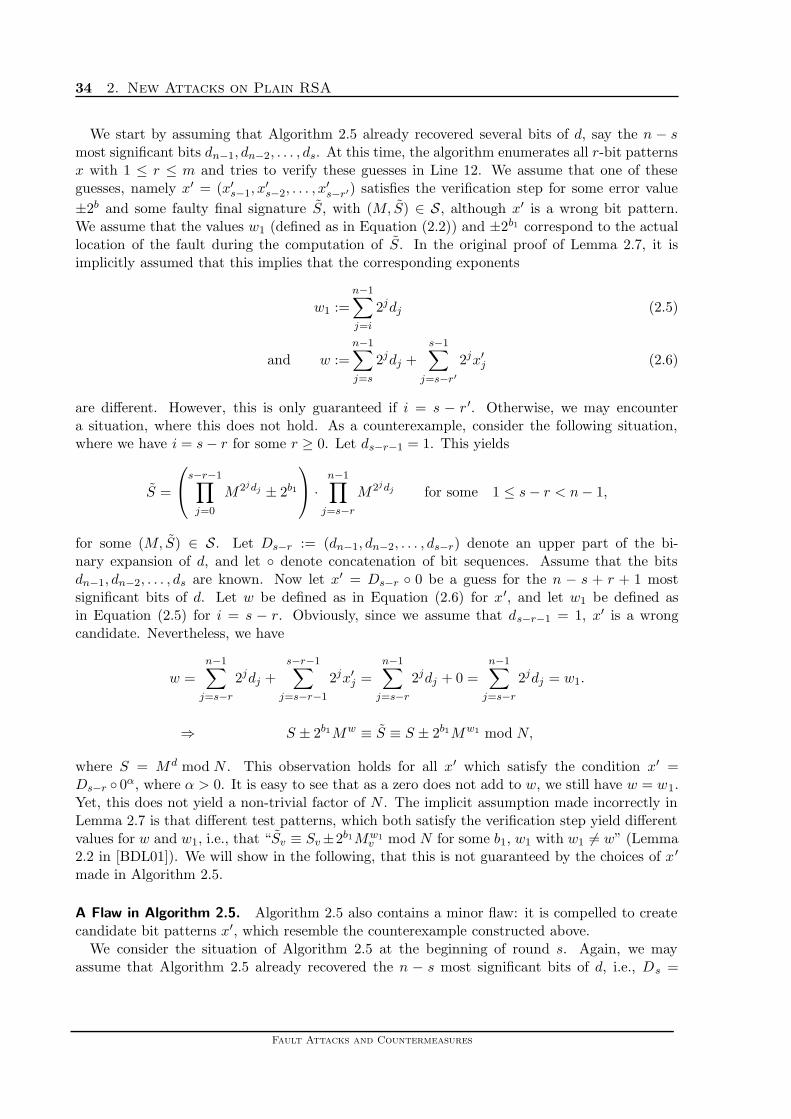
34 2. New Attacks on Plain RSA
We start by assuming that Algorithm 2.5 already recovered several bits of d, say the n − smost significant bits dn−1, dn−2, . . . , ds. At this time, the algorithm enumerates all r-bit patternsx with 1 ≤ r ≤ m and tries to verify these guesses in Line 12. We assume that one of theseguesses, namely x′ = (x′
s−1, x′s−2, . . . , x
′s−r′) satisfies the verification step for some error value
±2b and some faulty final signature S, with (M, S) ∈ S, although x′ is a wrong bit pattern.We assume that the values w1 (defined as in Equation (2.2)) and ±2b1 correspond to the actuallocation of the fault during the computation of S. In the original proof of Lemma 2.7, it isimplicitly assumed that this implies that the corresponding exponents
w1 :=
n−1∑
j=i
2jdj (2.5)
and w :=
n−1∑
j=s
2jdj +
s−1∑
j=s−r′
2jx′j (2.6)
are different. However, this is only guaranteed if i = s − r ′. Otherwise, we may encountera situation, where this does not hold. As a counterexample, consider the following situation,where we have i = s − r for some r ≥ 0. Let ds−r−1 = 1. This yields
S =
s−r−1∏
j=0
M2jdj ± 2b1
·
n−1∏
j=s−r
M2jdj for some 1 ≤ s − r < n − 1,
for some (M, S) ∈ S. Let Ds−r := (dn−1, dn−2, . . . , ds−r) denote an upper part of the bi-nary expansion of d, and let ◦ denote concatenation of bit sequences. Assume that the bitsdn−1, dn−2, . . . , ds are known. Now let x′ = Ds−r ◦ 0 be a guess for the n − s + r + 1 mostsignificant bits of d. Let w be defined as in Equation (2.6) for x′, and let w1 be defined asin Equation (2.5) for i = s − r. Obviously, since we assume that ds−r−1 = 1, x′ is a wrongcandidate. Nevertheless, we have
w =
n−1∑
j=s−r
2jdj +
s−r−1∑
j=s−r−1
2jx′j =
n−1∑
j=s−r
2jdj + 0 =
n−1∑
j=s−r
2jdj = w1.
⇒ S ± 2b1Mw ≡ S ≡ S ± 2b1Mw1 mod N,
where S = Md mod N . This observation holds for all x′ which satisfy the condition x′ =Ds−r ◦ 0α, where α > 0. It is easy to see that as a zero does not add to w, we still have w = w1.Yet, this does not yield a non-trivial factor of N . The implicit assumption made incorrectly inLemma 2.7 is that different test patterns, which both satisfy the verification step yield differentvalues for w and w1, i.e., that “Sv ≡ Sv ±2b1Mw1
v mod N for some b1, w1 with w1 6= w” (Lemma2.2 in [BDL01]). We will show in the following, that this is not guaranteed by the choices of x ′
made in Algorithm 2.5.
A Flaw in Algorithm 2.5. Algorithm 2.5 also contains a minor flaw: it is compelled to createcandidate bit patterns x′, which resemble the counterexample constructed above.
We consider the situation of Algorithm 2.5 at the beginning of round s. Again, we mayassume that Algorithm 2.5 already recovered the n − s most significant bits of d, i.e., Ds =
Fault Attacks and Countermeasures

2.1: The Differential Fault Attack on Right-To-Left Repeated Squaring 35
(dn−1, dn−2, . . . , ds). According to the verification step, Line 12, this implies that these n − sbits must have been recovered using the correct guess for the n− s most significant bits and thecorrect guess for the error term ±2b, together with some pair (Mj , Sj) ∈ S, 1 ≤ j ≤ #S, suchthat
(Sj ± 2b1Mw1
j
)e≡ Mj mod N, where w1 :=
n−1∑
j=s
2jdj . (2.8)
In the next round of Algorithm 2.5, all r-bit vectors x = (xs−1, xs−2, . . . , xs−r) are tested startingwith r = 1. Naturally, one would enumerate all bit vectors starting with the bit vector x = 0,followed by x = 1, x = 00, x = 01, x = 10, x = 11, etc. In [BDL01], no restriction on the choiceof the bit pattern x is mentioned. Algorithm 2.5 now starts with x = 0, guesses a value ±2b forthe error and tests all faulty signatures (Mj , Sj) ∈ S. In [BDL01], it is not mentioned that pairs,which have already been used to recover a fraction of d are removed from the set S, therefore,we assume that we try all faulty pairs (Mj , Sj) ∈ S again. At one time, the same (Mj , Sj) andthe same ±2b1 as in Equation (2.8) are tested. In this case, we have that w is build with the bitpattern Ds ◦ 0, which represents the counterexample above. If ds−1 = 1, a wrong bit pattern isaccepted, since we have
(S ± 2b1Mw
j
)e≡ Mj mod N, where w :=
n−1∑
j=s
2jdj +
s−1∑
j=s−r
2jxj = w1 + 0 = w1. (2.9)
But even worse: if the algorithm continues in the way described, it will now guess that allsuccessive bits are zero, because Equation (2.9) holds for any sequence x, which consists of zerosonly. This implies that once some leading bits have been recovered, no more non-zero bits willbe recovered correctly. Moreover, whenever a guess x satisfies the test in Equation (2.9), allother bit strings which are equal to x followed by an arbitrary number of zeros, would also beaccepted as correct guesses.
The algorithm fails due to two problems. First, zero bit strings x may be tested, which leadto erroneously verified bit patterns. Second, faulty signatures Sj, which have been used before,stay in the set S and are tested again in the next round. This shows that Algorithm 2.5 is notcorrect in the compact form stated in [BDL01].
We will show now that both, the proof of Lemma 2.7 and Algorithm 2.5 can be fixed easily.
2.1.2. Correcting Algorithm 2.5 and Lemma 2.7.
In order to fix Algorithm 2.5, we need to ensure that no zero postfixes occur. Trivially, this canbe achieved by demanding that only bit patterns x are tested which end with the digit 1. Thischoice guarantees that every new candidate x represents a new partial exponent w. Therefore,it may no longer happen that an old faulty value is redetected in the way described in Equation(2.9). We will show that this requirement also ensures that Lemma 2.7 holds. Although thenew restriction on x appears as a trivial modification at first sight, a new problem is created.Assume that from bit position s − 1 through s − m all bits of d are equal to zero. In the caseof such zero blocks, the correct bit pattern x would never be tested under the new requirementand Algorithm 2.5 would not come up with a valid guess. Fortunately, this is a problem, whichcan be solved with some additional considerations: we will show that setting the next bit to 0if no matching pattern is found will solve this problem. However, this situation requires specialattendance and will be formalized in Definition 2.8.
Martin Otto, Dissertation, December 2004

36 2. New Attacks on Plain RSA
Definition 2.8 (Zero Block Failure for Algorithm 2.3).Let x = (xn−1, xn−2, . . . , x0) be a positive integer with n := l(x), and let x′ = (xj−1, xj−2, . . . ,xj−m), m ≤ j ≤ n, be a block of m bits in x. Assume that faults are induced during the executionof the right-to-left repeated squaring algorithm, Algorithm 2.3. If all faults, which have beeninduced during iterations j −1, j −2, . . . , j −m, are restricted to iterations j −1, j −2, . . . , j − r,1 ≤ r ≤ m, where xj−1 = xj−2 = . . . = xj−r = 0, the situation is called a Zero Block Failure.We assume that at least one fault was induced during the iterations j − 1, j − 2, . . . , j − m.
A Zero Block Failure is named after the fact that errors in a block of zeros will not be detectedas errors within that block. Assume that S1 and S2 are two faulty values returned by Algorithm2.3 while being under attack. Let i1 and i2 denote the iterations, in which faults were inducedinto the intermediate value y. We assume w.l.o.g. that i2 ≤ i1. We further assume that the valuey on the right side of Line 4 is affected by the induced fault, i.e., prior to the multiplication withz. We denote by e1 and e2 the errors inflicted during the computation of S1 and S2 respectively.We have
S1 =
i1−1∏
j=0
m2jdj + e1
·
n−1∏
j=i1
m2jdj (2.10)
and S2 =
i2−1∏
j=0
m2jdj + e2
·
n−1∏
j=i2
m2jdj . (2.11)
Equations (2.10) and (2.11) show that if e1 = e2 and di2 = di2+1 = . . . = di1−1 = 0, it holdsthat S1 = S2. This is trivial since whenever di = 0, we have a factor of 1 in any of the products.Therefore, if two faults are induced within a zero block of bits and the error values e1 and e2 areequal, the two results cannot be distinguished. If the bits are recovered starting from the mostsignificant bit, it is not possible to determine how many zero bits — if any — follow the lastdetected 1. Any error induced in iterations j > i2 where it holds that dj = dj−1 = . . . = di2 = 0will be detected as S2 if the error e2 is the same as e1. Hence, tailing zeros must be neglected,because their number cannot be determined correctly. However, the fact that tailing zeros donot change the value of S allows us to write
S =
i−1∏
j=0
m2jdj + e2
·
n−1∏
j=i
m2jdj with di = 1, (2.12)
for some unknown i. Moreover, if it is known that the error happened in a certain iteration k,we may specify i in greater detail: here, we have i := max{j | dj = 1 ∧ j ≥ k}. The case whereS = S ± 2b, i.e., when k = n − 1 and the maximum does not exist, will be neglected, becauseit cannot yield any information. Any adversary can deliberately create values S ± 2b withoutknowing or learning anything about the secret key.
The above considerations about Zero Block Failures show that whenever such a Zero BlockFailure is encountered, our new algorithm would not be able to guess a correct value for thenext block of m bits. However, we may interpret a missing valid guess as an indicator for a ZeroBlock Failure. As a Zero Block Failure implies that at least a single zero occurs, we are able torecover the first following bit, which must be 0. As before, our indicator will be wrong at leastonce during Algorithm 2.9 with probability at most 1/2. This happens in the case when noneof the c = (n/m) log(2n) induced faults happened in the block of m bits under investigation.
Fault Attacks and Countermeasures

2.1: The Differential Fault Attack on Right-To-Left Repeated Squaring 37
The considerations explained above allow us to present the corrected Algorithm to attack theright-to-left repeated squaring algorithm. The modified parts compared to Algorithm 2.5 havebeen highlighted. We will prove the success probability afterwards.
Algorithm 2.9: Attack on Right-To-Left Repeated Squaring, Corrected Version
Input: Access to Algorithm 2.3, n the maximal length of the secret key d, e the RSA public key,m a parameter for acceptable amount of offline work.
Output: The secret key d with probability at least 1/2.
# Phase 1: Collect Faulty Outputs1 Set c := (n/m) · log(2n)2 Create c faulty outputs of Algorithm 2.3 on inputs Mi by inducing faults according to Fault
Model 1.7 in the intermediate variable y in random iterations.
3 Collect the set S = {(Mi, Si)| Mi an input to Algorithm 2.3 and Si a faulty output}.# Phase 2: Inductive Retrieval of Secret Key Bits4 Set s := n representing the index of the highest known bit of d.5 While (s > 0) do
# Compute the known MSB part of the exponent d.
6 Set ws :=∑n−1
j=s 2jdj
# Try all possible bit pattern with length r ≤ m.7 For all lengths r = 1, 2, . . . m do
8 For all candidate r-bit vectors x = (xs−1, xs−2, . . . xs−r+1, 1 ) of length r do# Compute the test candidate w
9 Set w := ws +∑s−1
j=s−r 2jxj
# Verification Step: Verify the test candidate using Equation (2.1)
10 for all (Mj, Sj) ∈ S do11 For all b from 0 to n − 1 do
12 if(Sj ± 2bMw
j
)e
≡ Mj mod N then
13 conclude that dj = xj for all s − r ≤ j ≤ s − 1,
14 delete (Mj, Sj) from the set S,
15 set s := s − r and continue at Line 5
# Handle a Zero Block Failure
16 If no test candidate satisfied the verification step, then
17 assume that ds−1 = 0 and set s := s − 1.
18 Output d
Remark. Algorithm 2.9 has been abbreviated in a minor detail. We base the success of Al-gorithm 2.9 on the “lucky case” of Fact 2.4. However, we are not guaranteed that a fault wasinduced during the first iteration i = 0 of the repeated squaring algorithm. We can recover bitsof d up to the lowest iteration, in which Algorithm 2.3 ever suffered a fault. This implies thateven in the “lucky case” of Fact 2.4, we may not be able to recover the m − 1 least significantbits of d in the manner described by Algorithm 2.9. However, since 2m operations represent anacceptable amount of offline work, it is possible to recover those m−1 least significant bits withexhaustive search. Note that this consideration also applies to the original version, Algorithm2.5.
Martin Otto, Dissertation, December 2004

38 2. New Attacks on Plain RSA
Since including the special case mentioned above would add complexity at a significant lossin clarity, we decided to state the attack algorithm in the abbreviated form.
Algorithm 2.9 is very similar to the original version, Algorithm 2.5. The difference is the newchoice of the test bit pattern x, which must end with the digit 1 now and, as a consequence,the handling of Zero Block Failures in Lines 16 and 17. We will now prove that this correctionyields a correct and successful attack on the right-to-left repeated squaring algorithm. First,we investigate the situation encountered at each round of Algorithm 2.9, i.e., at each time, theloop counter s is decreased. We will first show that if no valid candidate pattern x is foundwhich satisfies the verification step in Line 12 of Algorithm 2.9, a Zero Block Failure is correctlydetected. Then we will show that a false pattern will satisfy the verification step with negligibleprobability only. We conclude this section with an analysis of the running time of Algorithm2.9.
Lemma 2.10 (Correct Recovery).In each round s of Algorithm 2.9, we have one of three cases.
1. For some j, there is a block j − 1, j − 2, . . . , j − m of m contiguous iterations, during whichno fault was induced into the targeted variable.
2. Algorithm 2.9 finds a candidate bit vector x = (xs−1, xs−2, . . . , xs−r+1, 1) of length 1 ≤ r ≤m which satisfies the verification step in Line 12.
3. A Zero Block Failure is detected correctly, revealing the bit ds−1 = 0.
Proof:
The attack algorithm, Algorithm 2.9, relies on the assumption that Part 1 is false. If thereis a block of m iterations, such that no pair (Mv , Sv) ∈ S resulted from a fault induced intothe intermediate variable y during any of the m iterations, we do not claim that Algorithm2.9 will be able to recover d. However, as Fact 2.4 shows, this event occurs with probabilityat most 1/2. Therefore, we now assume that we have a “lucky case” and Part 1 is notsatisfied.
To show that a “lucky case” implies either Part 2 or Part 3, we now assume that Part 2is not satisfied. We claim that this implies that Part 3 is satisfied.
We assume that a certain round of Algorithm 2.9 is given, i.e., assume that the n− s mostsignificant bits dn−1, dn−2, . . . , ds of d are already known and Algorithm 2.9 now aims torecover the next 1 ≤ r ≤ m bits of d. If Part 2 is not satisfied, Algorithm 2.9 did not testany bit pattern of length 1 ≤ r ≤ m ending in the digit 1 successfully. We define
r′ := max{r | s − 1 ≤ s − r ≤ s − m and y has been hit by a fault during iteration r}.
Since we assume that Part 1 is not satisfied, we know that at least one of the intermediatevariables y computed during iterations s− 1, s− 2, . . . , s−m has been hit by a fault. Thisimplies that r′ exists and that 1 ≤ r′ ≤ m.
A Zero Block Failure is correctly detected if all bits ds−1, ds−2, . . . , ds−r′ are equal to zero,and in this case Algorithm 2.9 correctly recovers the next bit ds−1 = 0. If a Zero BlockFailure is detected incorrectly, there is at least one bit ds−k = 1 with 1 ≤ k ≤ r′. We now
Fault Attacks and Countermeasures

2.1: The Differential Fault Attack on Right-To-Left Repeated Squaring 39
assume that a Zero Block Failure is detected incorrectly and choose k to be maximal, i.e.,s − k is minimal and closest to s − r′. This implies that
s−k−1∑
j=s−r′
dj2j =
s−k−1∑
j=s−r′
0 · 2j = 0.
We consider the pair (Mv , Sv) ∈ S, which resulted from a fault induced into the interme-diate variable y during iteration s − r ′. Consider the test bit string x = (ds−1, ds−2, . . . ,ds−k+1, 1) of length 1 ≤ k ≤ r′ ≤ m. Obviously, x is one of the test patterns chosen in Line8. Let es−r′ denote the fault which has been induced. Given es−r′ , Sv, Sv = Md
v mod N ,and x, we have
Sv =
s−r′−1∏
j=0
M2jdjv + es−r′
·
s−k−1∏
j=s−r′
M2jdjv ·
n−1∏
j=s−k
M2jdjv
=
s−k−1∏
j=0
M2jdjv + es−r′
·
n−1∏
j=s−k
M2jdjv = Sv + es−r′ ·
n−1∏
j=s−k
M2jdjv = Sv + es−r′ · Mw
v ,
where w :=
n−1∑
j=s−k
2jdj as in Line 9 of Algorithm 2.9.
⇒(Sv − es−r′ · Mw
v
)e≡ Mv mod N. (2.14)
Equation (2.14) shows that the pattern x satisfies the verification step. However, thiscontradicts our assumption that Part 2 was false and Algorithm 2.9 did not find a satisfyingbit pattern. Therefore, if Part 2 is not satisfied, then a Zero Block Failure cannot bedetected incorrectly. This proves the lemma. �
Lemma 2.10 shows that if our basic assumption, the “lucky case” of Fact 2.4, is true, thenZero Block Failures are always detected correctly. It remains to show that Algorithm 2.9 alsorecovers bits of d correctly, if a satisfying bit pattern x is found. Although it is not impossiblethat a false bit pattern satisfies the verification step and is mistaken as the the correct pattern,Lemma 2.7 shows that such a false positive occurs with negligible probability only. Since weconsider the original proof of Lemma 2.7 to be not convincing in several details, we present adifferent approach here. It relies on the following two lemmas, which we will use again later inthis chapter.
Lemma 2.11 (Factorization with Polynomials Having Many Roots).Let N = p · q be an n-bit RSA modulus. Let W be a set of polynomials p(t) = tw − a ∈ ZN [t],with w ≤ 2N for all w. Furthermore, let #W < nτ for some constant τ > 0. Let δ > 0 be apositive constant. In this case, at least one of the following cases holds:
1. The probability that a random M ∈ ZN is a root of at least one of the #W many polyno-mials p(t) is less than 1/nδ.
2. A non-trivial factor of N can be computed in expected polynomial time.
Martin Otto, Dissertation, December 2004
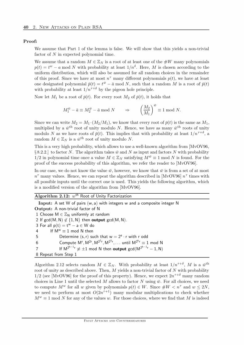
40 2. New Attacks on Plain RSA
Proof:
We assume that Part 1 of the lemma is false. We will show that this yields a non-trivialfactor of N in expected polynomial time.
We assume that a random M ∈ ZN is a root of at least one of the #W many polynomialsp(t) = tw − a mod N with probability at least 1/nδ. Here, M is chosen according to theuniform distribution, which will also be assumed for all random choices in the remainderof this proof. Since we have at most nτ many different polynomials p(t), we have at leastone designated polynomial p(t) = tw − a mod N , such that a random M is a root of p(t)with probability at least 1/nτ+δ by the pigeon hole principle.
Now let M1 be a root of p(t). For every root M2 of p(t), it holds that
M w1 − a ≡ M w
2 − a mod N ⇒(
M2
M1
)w
≡ 1 mod N.
Since we can write M2 = M1 ·(M2/M1), we know that every root of p(t) is the same as M1,multiplied by a wth root of unity modulo N . Hence, we have as many wth roots of unitymodulo N as we have roots of p(t). This implies that with probability at least 1/nτ+δ, arandom M ∈ ZN is a wth root of unity modulo N .
This is a very high probability, which allows to use a well-known algorithm from [MvOV96,§ 8.2.2.] to factor N . The algorithm takes w and N as input and factors N with probability1/2 in polynomial time once a value M ∈ ZN satisfying M w ≡ 1 mod N is found. For theproof of the success probability of this algorithm, we refer the reader to [MvOV96].
In our case, we do not know the value w, however, we know that w is from a set of at mostnτ many values. Hence, we can repeat the algorithm described in [MvOV96] nτ times withall possible inputs until the correct one is used. This yields the following algorithm, whichis a modified version of the algorithm from [MvOV96].
Algorithm 2.12: wth Root of Unity Factorization
Input: A set W of pairs (w, a) with integers w and a composite integer N
Output: A non-trivial factor of N1 Choose M ∈ ZN uniformly at random2 If gcd(M,N) 6∈ {1,N} then output gcd(M,N).3 For all p(t) = tw − a ∈ W do4 If Mw ≡ 1 mod N then5 Determine (s, r) such that w = 2s · r with r odd
6 Compute Mr,M2r,M22r,M23r, . . . until M2kr ≡ 1 mod N
7 If M2k−1r 6≡ ±1 mod N then output gcd(M2k−1r − 1,N)8 Repeat from Step 1
Algorithm 2.12 selects random M ∈ ZN . With probability at least 1/nτ+δ , M is a wth
root of unity as described above. Then, M yields a non-trivial factor of N with probability1/2 (see [MvOV96] for the proof of this property). Hence, we expect 2nτ+δ many randomchoices in Line 1 until the selected M allows to factor N using w. For all choices, we needto compute Mw for all w given by polynomials p(t) ∈ W . Since #W < nτ and w ≤ 2N ,we need to perform at most O(2nτ+1) many modular multiplications to check whetherMw ≡ 1 mod N for any of the values w. For those choices, where we find that M is indeed
Fault Attacks and Countermeasures
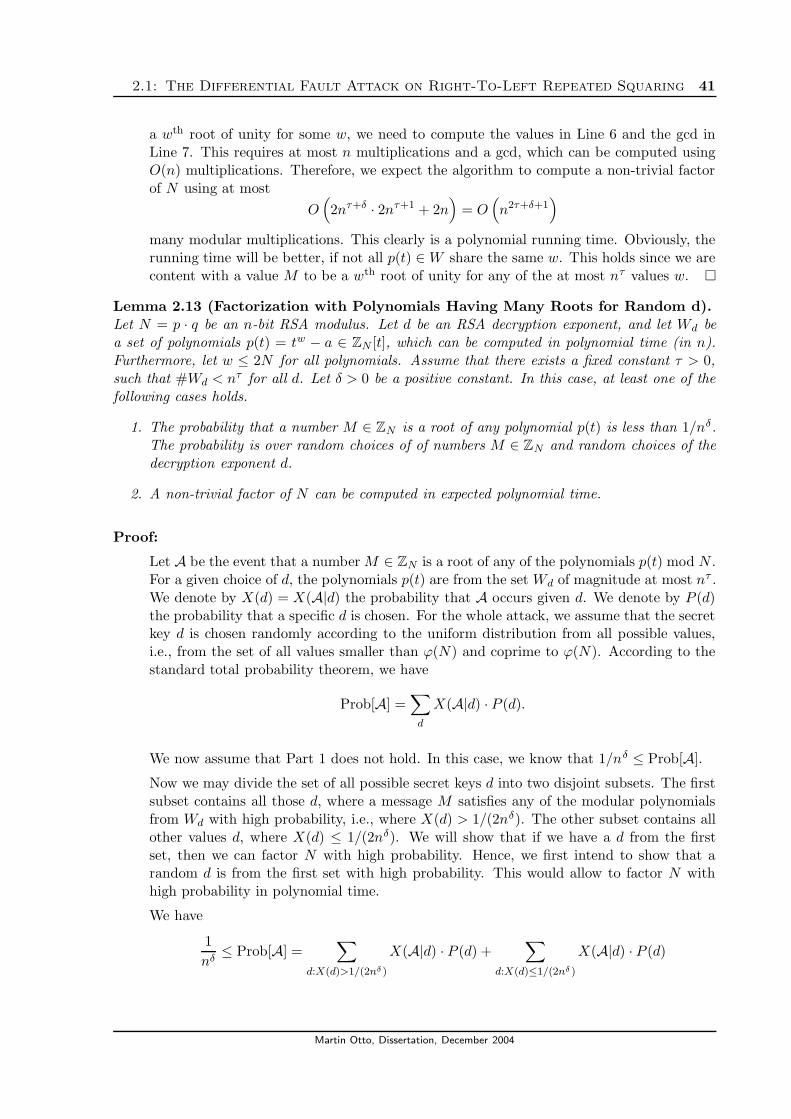
2.1: The Differential Fault Attack on Right-To-Left Repeated Squaring 41
a wth root of unity for some w, we need to compute the values in Line 6 and the gcd inLine 7. This requires at most n multiplications and a gcd, which can be computed usingO(n) multiplications. Therefore, we expect the algorithm to compute a non-trivial factorof N using at most
O(2nτ+δ · 2nτ+1 + 2n
)= O
(n2τ+δ+1
)
many modular multiplications. This clearly is a polynomial running time. Obviously, therunning time will be better, if not all p(t) ∈ W share the same w. This holds since we arecontent with a value M to be a wth root of unity for any of the at most nτ values w. �
Lemma 2.13 (Factorization with Polynomials Having Many Roots for Random d).Let N = p · q be an n-bit RSA modulus. Let d be an RSA decryption exponent, and let Wd bea set of polynomials p(t) = tw − a ∈ ZN [t], which can be computed in polynomial time (in n).Furthermore, let w ≤ 2N for all polynomials. Assume that there exists a fixed constant τ > 0,such that #Wd < nτ for all d. Let δ > 0 be a positive constant. In this case, at least one of thefollowing cases holds.
1. The probability that a number M ∈ ZN is a root of any polynomial p(t) is less than 1/nδ.The probability is over random choices of of numbers M ∈ ZN and random choices of thedecryption exponent d.
2. A non-trivial factor of N can be computed in expected polynomial time.
Proof:
Let A be the event that a number M ∈ ZN is a root of any of the polynomials p(t) mod N .For a given choice of d, the polynomials p(t) are from the set Wd of magnitude at most nτ .We denote by X(d) = X(A|d) the probability that A occurs given d. We denote by P (d)the probability that a specific d is chosen. For the whole attack, we assume that the secretkey d is chosen randomly according to the uniform distribution from all possible values,i.e., from the set of all values smaller than ϕ(N) and coprime to ϕ(N). According to thestandard total probability theorem, we have
Prob[A] =∑
d
X(A|d) · P (d).
We now assume that Part 1 does not hold. In this case, we know that 1/nδ ≤ Prob[A].
Now we may divide the set of all possible secret keys d into two disjoint subsets. The firstsubset contains all those d, where a message M satisfies any of the modular polynomialsfrom Wd with high probability, i.e., where X(d) > 1/(2nδ). The other subset contains allother values d, where X(d) ≤ 1/(2nδ). We will show that if we have a d from the firstset, then we can factor N with high probability. Hence, we first intend to show that arandom d is from the first set with high probability. This would allow to factor N withhigh probability in polynomial time.
We have
1
nδ≤ Prob[A] =
∑
d:X(d)>1/(2nδ )
X(A|d) · P (d) +∑
d:X(d)≤1/(2nδ )
X(A|d) · P (d)
Martin Otto, Dissertation, December 2004

42 2. New Attacks on Plain RSA
⇒ 1
nδ≤
∑
d:X(d)>1/(2nδ)
P (d) +1
2nδ
∑
d:X(d)≤1/(2nδ)
P (d) (2.18)
⇒ 1
2nδ≤
∑
d:X(d)>1/(2nδ)
P (d). (2.19)
Equation (2.18) holds, since X(d) is a probability, hence, 0 ≤ X(d) ≤ 1. This implies thatwe can replace all occurrences of X(d) by 1 in the first sum, which may not decrease theright hand side. For the second sum, we know that X(d) ≤ 1/(2nδ), hence, we do notdecrease the sum, if we replace each occurrence by the upper bound 1/(2nδ). Equation(2.19) follows from replacing the rightmost sum of probabilities P (d) in Equation (2.18)by the upper bound 1 and subtracting the resulting value 1/(2nδ). Equation (2.19) showsthat with probability at least 1/(2nδ), a randomly chosen d has X(A|d) ≥ 1/(2nδ) if Part1 is false.
In order to factor N , we subsequently choose values d and compute the set Wd. Eachpolynomial can be computed in polynomial time and since there are at most nτ polynomialsin each set Wd, the set Wd can be computed in polynomial time. We know that w is lessthan 2N . Given this data, we can apply Lemma 2.11, which shows that a non-trivialfactor of N can be computed in expected polynomial time. In Lemma 2.11, Part 2 appliesif the choice of d satisfies X(d) > 1/(2nδ). We know from the considerations above thatwe expect 2nδ random choices of decryption exponents d until X(d) > 1/(2nδ) is satisfied.This proves Part 2 of this lemma. �
We can now state the correct version of Lemma 2.7, which we will present as Lemma 2.14.
Lemma 2.14 (Accepting Wrong Candidates).Let δ > 0 be a fixed constant. For all n-bit RSA moduli N = p · q at least one of the followingclaims holds:
1. The probability that a wrong candidate x′ passes the test of Line 12 in Algorithm 2.9 isless than 1/nδ. The probability is over the random choices of messages Mi ∈ ZN given tothe attack algorithm and the random choice of the decryption exponent d.
2. A non-trivial factor of N can be computed in expected polynomial time (in n and 2m).
Proof:
We show an algorithm that factors all RSA moduli N for which Part 1 is false. The algo-rithm works as follows: it picks a random exponent d and random messages M1, . . . ,Mc ∈ZN . We have c = (n/m) log(2n) as in Fact 2.4. It then computes erroneous signatures Si
of the Mi by using the exponentiation algorithm (Algorithm 2.3) to compute M di mod N
and deliberately simulating a bit fault according to Fault Model 1.7 at a random iteration.Let (Mi, Si)
ci=1 be the resulting set of faulty signatures. We show there is a polynomial
time (in n and 2m) algorithm that given this data succeeds in factoring N with probabilityat least 1/nδ .
Fault Attacks and Countermeasures

2.1: The Differential Fault Attack on Right-To-Left Repeated Squaring 43
Computing the Set Wd. Suppose the attack algorithm was given (Mi, Si)ci=1 as input.
By assumption, with probability at least 1/nδ , at some point during the algorithm asignature Sv will incorrectly cause the wrong candidate x′ to be accepted in Step 12. Thatis, Sv ± 2bMw
v ≡ Sv mod N even though Sv was generated by a different fault (here w isdefined as in Step 9 using the bits of x′). We know that Sv ≡ Sv ± 2b1Mw1
v mod N forsome b1, w1. The pair b1, w1 corresponds to the actual location of the fault during thecomputation of Sv.
Now we claim that we have w 6= w1. We know that any bit pattern x = (dn−1, dn−2, . . . ,ds, xs−1, xs−2, . . . , xs−r), which satisfies the verification step, ends in the digit 1. Sincethe leading digit is dn−1 = 1, no digits on either end vanish by not contributing to thevalue w. The value w1 is computed as w1 =
∑n−1j=i dj2
j . If i > s−r, we know that w 6= w1,
since the addend 2s−rxs−r with xs−r = 1 is not added to w1. This cannot be corrected bychoosing any different pattern for the bits (xs−1, xs−2, . . . , xs−r+1) due to the nature of thebinary expansion. If i = s − r, we have w = w1 iff x represents the correct bit pattern ofd, because both are of the same length. If i < s− r, we may have w = w1 if all bits dj = 0for i ≤ j < s− r. However, we only claim that x represents the correct bit pattern for then − s + r most significant bits, we do not recover any additional bits. Hence, we do notneed to consider other bits as long as our guessed pattern is correct for the correspondingsubpattern of d. If any of the bits dj = 1 for i ≤ j < s− r, we clearly have w 6= w1. Henceit is true that if x′ is a wrong bit pattern, w and w1 are bound to be different.
As explained before, w 6= w1 implies that we have
S ± 2b1Mw1 ≡ S ± 2bMw mod N.
Rearranging terms we get Mw−w1 ≡ ±2b1−b mod N . In other words, M must be a root ofa polynomial of the form
tw−w1 ≡ a mod N
for some known constant a = ±2b1−b. We now define the set Wd to be the set ofall polynomials of the form p(t) = tw−w1 ± 2b1−b mod N , which may occur during anattack. We ensure positive exponents, hence, if w < w1, we consider the equationtw1−w ≡ ±2b−b1 mod N .
We wish to apply Lemma 2.13 to show that Part 2 of this lemma must hold if Part 1 isfalse. First, we need to bound the number of polynomials p(t) = tω − a mod N , whereω = w − w1 and a = ±2b1−b. The value of w1 is essentially the prefix of d from the mostsignificant bit to the fault location. We have at most n + 1 prefixes of a bit sequenceof length n, however, at most n apply in our case, since the main loop in the right-to-left repeated squaring algorithm, Algorithm 2.3, is executed only n times, hence, only ndifferent intermediate values y can be affected by a fault. The values of w are the onestested in Step 12. There are at most n · (2m+1 − 2) < 2n · 2m possible values, since wcomprises of known upper bits of d and at most m guessed bits. Hence, there are 2n22m
possible values for ω = w −w1. For the values b and b1, there are at most 2n possibilities.Hence, a can take at most 2n2 many values, since the signs of ±2b and ±2b1 may either bethe same or not. Hence, there are at most 4n42m many different polynomials p(t). Sinceevery polynomial can be computed in polynomial time, the set Wd can be constructed inpolynomial time.
Martin Otto, Dissertation, December 2004

44 2. New Attacks on Plain RSA
Factoring N. By assumption, Part 1 of the lemma is false. Hence, with probability atleast 1/nδ (over the choice of d and M) we have that a randomly chosen value M ∈ZN satisfies any of the polynomials p(t) = tω − a mod N . Note that ω depends on thechoice of d. We have shown that for any d, there are at most 4n42m many polynomialsp(t) = tω − a mod N in Wd, and Wd can be computed in polynomial time given d. Forτ = m+5, we guarantee #Wd < nτ . Clearly, we have ω ≤ 2N , since both w and w1 satisfy2n−1 ≤ w,w1 ≤ 2n − 1, hence, ω = w − w1 < 2n−1 < N . Hence, the condition ω ≤ 2N issatisfied. Since we have shown that acceptance of a wrong candidate implies that at leastone of the polynomials p(t) is satisfied, and we assume that this holds with probability atleast 1/nδ, we may use Lemma 2.13 now. Since Part 2 of Lemma 2.13 holds, we can factorN in expected polynomial time. This proves Part 2 of this lemma. �
The two lemmas 2.10 and 2.14 allow to state the following theorem, proving that the correctedattack algorithm has a high probability to recover the secret key d. Therefore, the flaw in[BDL01] can easily be fixed. The important contribution of [BDL01], starting off research infault attacks, remains valid.
Theorem 2.15 (Corrected Attack on RSA by Boneh, DeMillo, and Lipton).Let N = p · q be an n-bit RSA modulus. For any 1 ≤ m ≤ n, given (n/m) log(2n) pairs(Mi, Si), the secret exponent d can be extracted from Algorithm 2.3 with probability at least 1/2.The probability is over the location of the register faults and random messages mi ∈ ZN . Thealgorithm’s running time is dominated by the time it takes to perform O((2mn3 log(n))/m) fullmodular exponentiations mod N .
Proof:
With probability 1/2 guaranteed by Fact 2.4, every contiguous m-bit interval is hit by afault at least once. Lemma 2.10 guarantees that in each round of the main loop (Lines4–17), either a candidate pattern is found or one bit is correctly recovered. Lemma 2.14guarantees that with a negligible loss in the success probability, any candidate patternfound represents the correct bit pattern, thus revealing at least one more bit of d. There-fore, the main loop is executed at most n = blog(N)c + 1 times. In every round, at most2m+1 − 2 different bit patterns x are tested together with at most 2n different errors andat most c = (n/m) log(2n) different pairs (Mv, Sv) ∈ S. Each test requires two modularexponentiations, one with the value w and one with the public key e. Hence, we have atotal of n · (2m+1 − 1) · 2n · (n/m) log(2n) · 2 = O(2mn3 log(n)/m) full modular exponenti-ations. The generation of the set S requires (n/m) log(2n) modular exponentiations withthe ability to induce a fault, which vanishes in the O-notation. �
Our analysis yields an asymptotic running time of O((2mn3 log(n))/m) modular exponentiations,while the original analysis presented as Theorem 2.6 yields an asymptotic running time ofO((2mn3 log2(n))/m2) modular exponentiations. This implies that our analysis yields a betterasymptotic running time than Theorem 2.6 if (log(n)/m)2 > log(n)/m, i.e., if log(n) > m,which is true for all practical choices of parameters. We achieve a better result due to a morecareful analysis: there are c different faulty results S, each of which may be used to reveal apart of d. However, at most n of them may yield different sub-patterns of d. If two faultyresults are generated by a fault attack during the same iteration, but with a different error, oneof them will never be used to recover a part of d. Obviously, if the first one has been used, thesecond one cannot yield additional information about d. Hence, we can replace one factor ofc = n · (log(2n)/m) by n. This explains the improved result.
Fault Attacks and Countermeasures
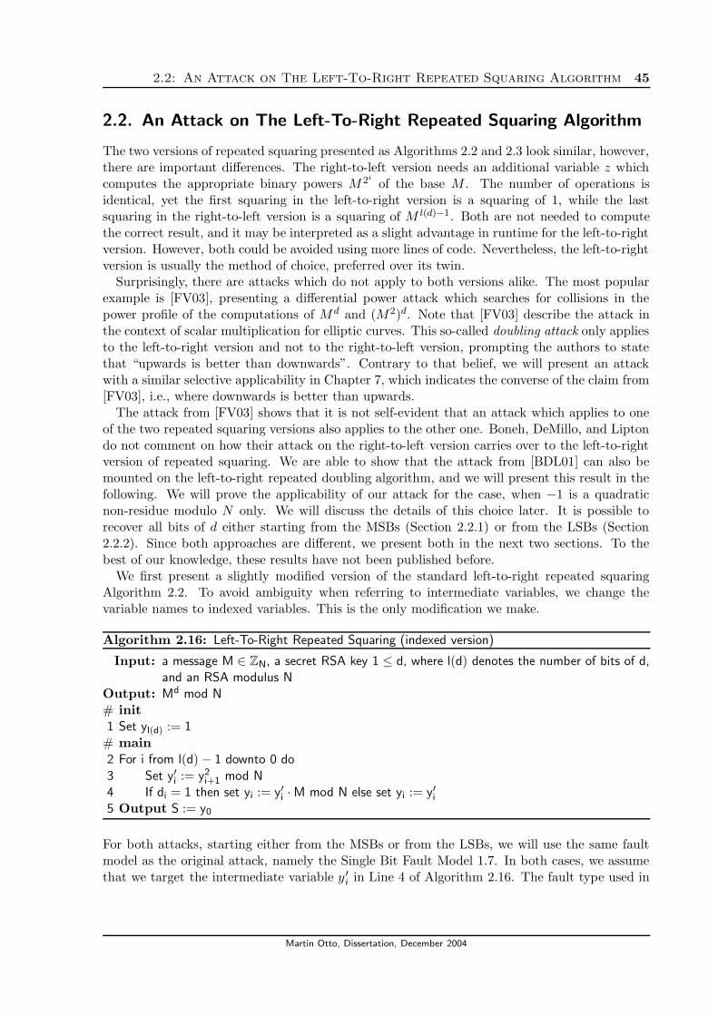
2.2: An Attack on The Left-To-Right Repeated Squaring Algorithm 45
2.2. An Attack on The Left-To-Right Repeated Squaring Algorithm
The two versions of repeated squaring presented as Algorithms 2.2 and 2.3 look similar, however,there are important differences. The right-to-left version needs an additional variable z whichcomputes the appropriate binary powers M 2i
of the base M . The number of operations isidentical, yet the first squaring in the left-to-right version is a squaring of 1, while the lastsquaring in the right-to-left version is a squaring of M l(d)−1. Both are not needed to computethe correct result, and it may be interpreted as a slight advantage in runtime for the left-to-rightversion. However, both could be avoided using more lines of code. Nevertheless, the left-to-rightversion is usually the method of choice, preferred over its twin.
Surprisingly, there are attacks which do not apply to both versions alike. The most popularexample is [FV03], presenting a differential power attack which searches for collisions in thepower profile of the computations of M d and (M2)d. Note that [FV03] describe the attack inthe context of scalar multiplication for elliptic curves. This so-called doubling attack only appliesto the left-to-right version and not to the right-to-left version, prompting the authors to statethat “upwards is better than downwards”. Contrary to that belief, we will present an attackwith a similar selective applicability in Chapter 7, which indicates the converse of the claim from[FV03], i.e., where downwards is better than upwards.
The attack from [FV03] shows that it is not self-evident that an attack which applies to oneof the two repeated squaring versions also applies to the other one. Boneh, DeMillo, and Liptondo not comment on how their attack on the right-to-left version carries over to the left-to-rightversion of repeated squaring. We are able to show that the attack from [BDL01] can also bemounted on the left-to-right repeated doubling algorithm, and we will present this result in thefollowing. We will prove the applicability of our attack for the case, when −1 is a quadraticnon-residue modulo N only. We will discuss the details of this choice later. It is possible torecover all bits of d either starting from the MSBs (Section 2.2.1) or from the LSBs (Section2.2.2). Since both approaches are different, we present both in the next two sections. To thebest of our knowledge, these results have not been published before.
We first present a slightly modified version of the standard left-to-right repeated squaringAlgorithm 2.2. To avoid ambiguity when referring to intermediate variables, we change thevariable names to indexed variables. This is the only modification we make.
Algorithm 2.16: Left-To-Right Repeated Squaring (indexed version)
Input: a message M ∈ ZN, a secret RSA key 1 ≤ d, where l(d) denotes the number of bits of d,and an RSA modulus N
Output: Md mod N# init1 Set yl(d) := 1
# main2 For i from l(d) − 1 downto 0 do
3 Set y′i := y2i+1 mod N
4 If di = 1 then set yi := y′i · M mod N else set yi := y′i5 Output S := y0
For both attacks, starting either from the MSBs or from the LSBs, we will use the same faultmodel as the original attack, namely the Single Bit Fault Model 1.7. In both cases, we assumethat we target the intermediate variable y ′
i in Line 4 of Algorithm 2.16. The fault type used in
Martin Otto, Dissertation, December 2004

46 2. New Attacks on Plain RSA
the Single Bit Fault Model is that of bit flip faults following Definition 1.3, which implies that wecan write the effect of the fault as y′
i 7−→E y′i ± 2b, for some random 0 ≤ b < l(y′i). For simplicity,
we assume that l(y′i) = l(N), i.e., even if y′
i is a number with less digits than the modulus,we assume that leading zeros can be flipped to 1 as well. If this is impossible in practice, ouralgorithm tests too many candidates for b, which is a negligible overhead. For the analysis ofour attack, we will use the following definitions.
Definition 2.17 (High and Low Parts of an Integer).Let d > 0 be an n-bit integer with binary expansion d = (dn−1, dn−2, . . . , d0). As d ≥ 1, we havedn−1 = 1. We define the high part hi(d) and the low part li(d) of d, build by the n − i mostsignificant and i + 1 least significant bits of d respectively, as
li(d) :=i∑
j=0
2jdj and hi(d) :=n−1∑
j=i
2j−idj (2.22)
⇒ d = 2i+1hi+1(d) + li(d) ∀ i ∈ Z. (2.23)
We will now derive some basic equations to describe the values of the intermediate variablesused in Algorithm 2.16 in greater detail.
Proposition 2.18 (Properties of the Variables Used in Algorithm 2.16).Let S := Md mod N and let S denote a faulty output of Algorithm 2.16 resulting from a faultinduced into the intermediate variable y ′
i for some 0 ≤ i ≤ n − 1. Let n = l(d) be the length ofthe secret key d ≥ 1, and let ei denote the error induced into the variable y ′
i. In this case, wehave the following equations for some of the variables computed by Algorithm 2.16:
y′i ≡ (((M2dn−1 · Mdn−2)2 · Mdn−3)2 · . . . · Mdi+1)2 ≡ M2hi+1(d) mod N (2.24)
(the intermediate value y′i from Algorithm 2.16 which is attacked)
yi ≡ (((M2dn−1 · Mdn−2)2 · Mdn−3)2 · . . . · Mdi+1)2 · Mdi ≡ y′i · Mdi ≡ Mhi(d) mod N
(the intermediate value yi from Algorithm 2.16 which is the result of round i)
S ≡ y′2i
i · M li(d) ≡(M2hi+1(d)
)2i
· M li(d) ≡ M2i+1hi+1(d)+li(d) ≡ Md mod N (2.25)
(the correct final result of Algorithm 2.16)
S ≡ (y′i + ei)2i · M li(d) mod N (2.26)
(the faulty final result of Algorithm 2.16)
Proof:
The formulas are easily derived from Algorithm 2.16. It is
yi = M� n−1
j=i 2j−idj ,
as yi always contains the result Mhi(d), since hi(d) = (dn−1, dn−2, . . . , di), i.e., the highpart of d. This value is squared in the next iteration to yield y ′
i−1 = y2i . Given yi and y′i,
Equations (2.25) and (2.26) follow directly using Equation (2.23). �
In the following, we will show that it is possible to recover all bits of d either starting from theMSBs or from the LSBs. The MSB approach is very similar to the original attack described in[BDL01]. However, the LSB version requires some additional work.
Fault Attacks and Countermeasures

2.2: An Attack on The Left-To-Right Repeated Squaring Algorithm 47
For both attacks, we assume that the RSA modulus N has been chosen to guarantee that −1is a quadratic non-residue modulo N . This means that there is no integer a ∈ ZN such thata2 ≡ −1 mod N . We will briefly discuss the possibility to generalize our attack to arbitrarymoduli N in Section 2.3. The restriction to these special moduli is practical. For example, theproperty that −1 is a quadratic non-residue holds for Blum integers, i.e., integers N = p ·q, suchthat both primes satisfy p, q ≡ 3 mod 4. If p and q are chosen as strong primes, i.e., primes pand q with the property that (p − 1)/2 and (q − 1)/2 are prime, N is guaranteed to be a Bluminteger. Choosing strong primes offers security against certain factorization algorithms, e.g.,Pollards p− 1 factoring algorithm [MvOV96, § 3.2.3]. We will discuss in Section 3.3.1 that suchstrong primes can be found efficiently. Hence, restricting our analysis to this case is reasonable.
Given the fact that −1 is a quadratic non-residue modulo N , we can use the following factabout 2ith congruences to ease our analyses.
Lemma 2.19 (2ith Congruence Factorization).Let x and y be integers and let N be a composite integer such that −1 is a quadratic non-residuemodulo N . If there is an integer i ≥ 1, such that
x2i ≡ y2i
mod N,
and x 6≡ ±y mod N , then there is a 0 ≤ k < i such that gcd(x2k − y2k, N) yields a non-trivial
factor of N .
Proof:
Assume that x 6≡ ±y mod N . Since x2i ≡ y2imod N , there must be a minimal k ≥ 0,
such that x2k+1 ≡ y2k+1
mod N and x2k 6≡ y2kmod N . This yields two cases, one where
x2k 6≡ ±y2kmod N , and a second where x2k ≡ −y2k
mod N .
Case 1. Assume that we have x2k 6≡ ±y2kmod N . Let a := x2k
and b := y2k. We have
a 6≡ ±b mod N but a2 ≡ b2 mod N . The latter implies that N | (a − b) · (a + b). Byassumption, both factors are not equal to zero and both factors are not multiples of N .Therefore, N must contain a non-trivial factor q, which divides (a − b) but not (a + b).
This factor can be computed by gcd(a − b,N) = gcd(x2k − y2k, N).
Case 2. Assume that we have x2k ≡ −y2kmod N . This implies that (x/y)2k ≡ −1 mod
N . The power k must be larger than 0, since we assume that x 6≡ ±y. Therefore, a squareroot of −1 is given by (x/y)2
k−1
. However, we assume that −1 is a quadratic non-residuemodulo N . Hence, Case 2 is impossible. �
2.2.1. Fault Attack Starting From the MSBs
In order to recover the bits of the secret key d starting from the MSBs, we need to derive adescription of a faulty final result S, which depends only on the most significant bits of d. Thiswill be the basis for our recovery. We state such an equation in the following lemma. In theremainder of this section, we will denote errors induced by a fault by ei, where i denotes theaffected iteration, and guessed values for the “correct error” ei by ε.
Martin Otto, Dissertation, December 2004
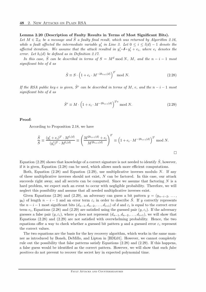
48 2. New Attacks on Plain RSA
Lemma 2.20 (Description of Faulty Results in Terms of Most Significant Bits).Let M ∈ ZN be a message and S a faulty final result, which was returned by Algorithm 2.16,while a fault affected the intermediate variable y ′
i in Line 3. Let 0 ≤ i ≤ l(d) − 1 denote theaffected iteration. We assume that the attack resulted in y ′
i 7−→E y′i + ei, where ei denotes theerror. Let hi(d) be defined as in Definition 2.17.
In this case, S can be described in terms of S = M d mod N , M , and the n − i − 1 mostsignificant bits of d as
S ≡ S ·(1 + ei · M−2hi+1(d)
)2i
mod N. (2.28)
If the RSA public key e is given, Se can be described in terms of M , e, and the n − i − 1 mostsignificant bits of d as
Se ≡ M ·(1 + ei · M−2hi+1(d)
)2iemod N. (2.29)
Proof:
According to Proposition 2.18, we have
S
S≡ (y′i + ei)
2i · M li(d)
(y′i)2i · M li(d)
≡(
M2hi+1(d) + ei
M2hi+1(d)
)2i
≡(1 + ei · M−2hi+1(d)
)2i
mod N.
�
Equation (2.29) shows that knowledge of a correct signature is not needed to identify S, however,if it is given, Equation (2.28) can be used, which allows much more efficient computations.
Both, Equation (2.28) and Equation (2.29), use multiplicative inverses modulo N . If anyof these multiplicative inverses should not exist, N can be factored. In this case, our attacksucceeds right away, and all secrets can be computed. Since we assume that factoring N is ahard problem, we expect such an event to occur with negligible probability. Therefore, we willneglect this possibility and assume that all needed multiplicative inverses exist.
Given Equations (2.28) and (2.29), an adversary can guess a bit pattern y = (yn−i−2, . . . ,y0) of length n − i − 1 and an error term εi in order to describe S. If y correctly representsthe n− i − 1 most significant bits (dn−1, dn−2, . . . , di+1) of d and εi is equal to the correct errorterm ei, Equations (2.28) and (2.29) are satisfied using the guessed pair (y, εi). If the adversaryguesses a false pair (y, εi), where y does not represent (dn−1, dn−2, . . . , di+1), we will show thatEquations (2.28) and (2.29) are not satisfied with overwhelming probability. Hence, the twoequations offer a way to check whether a guessed bit pattern y and a guessed error εi representthe correct values.
The two equations are the basis for the key recovery algorithm, which works in the same man-ner as introduced by Boneh, DeMillo, and Lipton in [BDL01]. However, we cannot completelyrule out the possibility that false patterns satisfy Equations (2.28) and (2.29). If this happens,a false guess would be identified as the correct pattern. However, we will show that such falsepositives do not prevent to recover the secret key in expected polynomial time.
Fault Attacks and Countermeasures

2.2: An Attack on The Left-To-Right Repeated Squaring Algorithm 49
We will now state the complete attack algorithm.
Algorithm 2.21: Attack on Left-To-Right Repeated Squaring, MSB Version
Input: Access to Algorithm 2.16, n the maximal length of the secret key d, e the RSA public key,m a parameter for acceptable amount of offline work.
Output: d with probability at least 1/2.# Phase 1: Collect Faulty Outputs1 Set c := (n/m) · log(2n)2 Create c faulty outputs of Algorithm 2.16 on inputs Mj by inducing faults according to Fault
Model 1.7 in the intermediate variable y′i in random iterations.
3 Collect the set S = {(Mj, Sj)| Mj an input to Algorithm 2.16 and Sj a faulty output}.# Phase 2: Inductive Retrieval of Secret Key Bits4 Set s := 0 representing the current candidate bit length between s · m + 1 and (s + 1) · m5 Set K := {ε} to contain candidates for verified/“known” MSB-parts of d6 While (s · m < n − 1) do7 for all patterns y = (yu−1, yu−2, . . . , y0) ∈ K with length u := l(y) do
# The algorithm ensures that (s − 1) · m < u ≤ s · m8 Set K′ = ∅ # to contain candidates of length between s · m + 1 and (s + 1) · m9 For all r with s · m < u + r ≤ (s + 1) · m do
10 For all test bit patterns x = (xr−1, xr−2, . . . x0) of length r < 2m do# Compute the test candidate w using the pattern y ◦ x
11 Set w := 2ru−1∑
j=0
yj2j +
r−1∑
j=0
xj2j
# Verification Step: Verify the test candidate using Equation (2.29)
12 For all (M, S) ∈ S do13 For all b from 0 to n − 1 do
14 if Se ≡ M ·(1 ± 2b · M−2w
)2u+r−1emod N then
15 Add y ◦ x = (yu−1, yu−2, . . . , y0, xr−1, . . . , x0) to the set K′
16 Set K := K′ and s := s + 1 and continue at Line 6# Phase 3: Compute k from all candidates of length u > n − 1 − m17 For all patterns y = (yu−1, yu−2, . . . , y0) ∈ K with length u := l(y) do18 Set r := n − 1 − u19 For all test bit patterns x = (xr−1, xr−2, . . . x0) of length r < m do
20 Set w := 2ru−1∑
j=0
yj2j +
r−1∑
j=0
xj2j
21 If Mw·e ≡ M mod N then Output (yu−1, yu−2, . . . , y0, xr−1, . . . , x0)22 Output FAILURE
The symbol ε used in Line 5 denotes the empty bit string of length 0.
Algorithm 2.21 consists of three phases. In the first phase, we collect up to c = (n/m) · log(2n)faulty values S. In Phase 2, the algorithm tries to recover the secret key d starting from the mostsignificant bits. Here, a “known” upper part y = (yu−1, yu−2, . . . , y0) is assumed to representthe u most significant bits (dn−1, dn−2, . . . , dn−u) of d. These known upper bits will be combinedwith all possible r-bit extensions to form test bit patterns. Each test bit pattern is tested using
Martin Otto, Dissertation, December 2004

50 2. New Attacks on Plain RSA
all possible faulty results from Phase 1, all possible error terms εi, and Equation (2.29). Since weassume the Single Bit Fault Model 1.7, we can enumerate all possible error values in polynomialtime. If Equation (2.29) is satisfied for any combination, a new “known” upper part of d hasbeen recovered.
However, a fundamental difference to the attack on right-to-left repeated squaring presented inthe beginning of this chapter is the existence of false positives. Since we will not show that falsepositives only occur with negligible probability, we must take the existence of false positives intoaccount. This implies that a “known” upper part may be a false guess. We solve this problemby collecting all known upper parts and by trying all of them to derive new longer patterns.Later, we will show that this strategy is feasible.
Phase 3 captures the special case when no error was induced into the last r < m iterations.At this time, at most m bits are unknown, hence, they can be recovered by exhaustive search.
Remark. Algorithm 2.21 has been abbreviated for clarity in one minor detail. Since we alwaysassume that d > 0, we know that dn−1 = 1. This implies that the algorithm should only testcandidate patterns, which start with the digit 1. This consideration could be incorporated bystarting the main loop of Lines 6–16 with setting K := {1} in Line 5. However, this featurerequires a more complicated description of the loop invariants, e.g., of (s − 1) · m < u ≤ s · m.Hence, omitting this consideration adds clarity. Nevertheless, the fact that dn−1 = yu−1 = 1will be used in the analysis later.
Algorithm 2.21 shows the same basic pattern as Algorithm 2.9, which was used for an attackon the right-to-left repeated squaring algorithm. The main difference is the use of a set Kto contain verified upper parts of d, allowing the occurrence of multiple verified candidate bitpatterns.
Another difference to Algorithm 2.9 is the absence of any Zero Block Failure handling. Algo-rithm 2.21 has no problem equivalent to the Zero Block Problem as defined in Definition 2.8,because the value
w = 2ru−1∑
j=0
yj2j +
r−1∑
j=0
xj2j
used in Line 10 of Algorithm 2.21 is build from the left to the right with the most significantbit yu−1 = 1. A tailing zero bit x0 = 0 does not vanish like in the case of Zero Block Failures, itshifts the leading bits by 1 to the left, thus changing the value of w. Hence, the pattern y ◦ x isa unique bit pattern, which uniquely encodes a positive integer w. Therefore, it is not possiblethat two different bit patterns yield the same integer w. This would only be possible if a patterny ◦ x was allowed to contain leading, i.e., leftmost, zeros. Therefore, no problem similar to theZero Block Failure introduced in Definition 2.8 may occur.
In the following, we will first investigate the occurrence of false positives in detail. This analysiswill allow us to state results about the success probability and the running time of Algorithm2.21. We start with defining valid guesses and formalizing the notion of false positives.
Fault Attacks and Countermeasures

2.2: An Attack on The Left-To-Right Repeated Squaring Algorithm 51
Definition 2.22 (Valid Guesses and False Positives in Algorithm 2.21).Let S = Md mod N be an RSA signature and let S be a faulty result as defined in Proposition2.18. Let y = (yu−1, yu−2, . . . , y0) be a bit pattern of length u with yu−1 = 1. This pattern yieldsa value w as used in Algorithm 2.21 according to the following formula:
w :=u−1∑
j=0
yj2j .
Let ε = ±2b, 0 ≤ b < n, be a guessed value for the error e(y ′n−u−1). If the verification step of
Algorithm 2.21 yields
Se
M≡(1 + ε · M−2w
)2n−u−1e,
then (y, ε) is called a valid guess for the bit pattern (dn−1, dn−2, . . . , dn−u) and the correct errore(y′n−u−1). If for at least one n− 2 ≥ j ≥ n − u it holds that dj 6= yj−n+u, the valid guess (y, ε)is called a false positive.
A false positive satisfies the verification step in Line 14 of Algorithm 2.21, yet it represents afalse bit pattern. A false positive only requires the bit pattern y to be wrong. We do not considerthe correctness of the error value ε. This is due to the fact that we do not need to learn thecorrect error value ei for ε in order to recover the bit pattern of the secret RSA key d.
We will now show that during the execution of Algorithm 2.21, the number of all bit patterns,which ever occur in the round sets K ′, does not exceed a certain bound with overwhelmingprobability.
Lemma 2.23 (Bounding the Number of Special Valid Guesses).Let Ks be the round set K computed in Line 16 at iteration s of the main loop of Algorithm2.21 (Lines 6–16). Let −1 be a quadratic non-residue modulo N , c = (n/m) log(2n), and let
κ :=∑
j
#Kj.
If κ > 2nc, then at least one of the following cases holds:
1. There are two valid guesses (x, εx) and (y, εy) with x 6= y such that
(1 + εx · M−2wx
)≡
(1 + εy · M−2wy
)mod N
where wx :=
l(x)−1∑
j=0
xj2j and wy :=
l(y)−1∑
j=0
yj2j .
2. There are two valid guesses (x, εx) and (y, εy) with x 6= y such that
gcd((
1 + εx · M−2wx)2k
−(1 + εy · M−2wy
)2k
, N)∈ {p, q},
for a 0 ≤ k ≤ n − u − 1 with u = l(x) = l(y), and wx and wy as defined in Case 1.
Martin Otto, Dissertation, December 2004

52 2. New Attacks on Plain RSA
Proof:
We assume that κ ≥ 2nc + 1. This implies that there are at least 2nc + 1 different bitpatterns y in the union of all Ks. This is true since elements from different round sets Ks
have a different bit length, hence, there cannot be one pattern in multiple round sets. Forevery such y, there exists an εy, such that (y, εy) is a valid guess, which has been generatedand tested by Algorithm 2.21 in Line 14. In this case, we can use the pigeon hole principleto show that there must be at least one pair (M, S) ∈ S such that 2n + 1 of these validguesses were verified using (M, S). We now fix this pair (M, S).
Since we have at least 2n + 1 many valid guesses, but only n possible values for thebit lengths of the bit patterns y, we have at least three valid guesses with the same bitlength u. We denote these three valid guesses by (x, εx), (y, εy), and (z, εz). We havel(x) = l(y) = l(z) = u, and we denote the bits of all three patterns starting with the indexu − 1 through 0. In this case, Definition 2.22 shows that we have
Se
M≡(1 + εx · M−2wx
)2n−u−1e
≡(1 + εy · M−2wy
)2n−u−1e
≡(1 + εz · M−2wz
)2n−u−1emod N.
Since gcd(e, ϕ(N)) = 1, exponentiation with e is a bijection, hence, we have
(1 + εx · M−2wx
)2n−u−1
≡(1 + εy · M−2wy
)2n−u−1
≡(1 + εz · M−2wz
)2n−u−1
. (2.32)
Equation (2.32) allows to factor N unless we have
(1 + εx · M−2wx
)≡ ±
(1 + εy · M−2wy
)≡ ±
(1 + εz · M−2wz
), (2.33)
according to Lemma 2.19. Note that we assume that −1 is a quadratic non-residue moduloN , hence, Lemma 2.19 can be applied. This shows that either Equation (2.33) or Case 2of Lemma 2.23 holds, i.e., N can be factored with the claimed gcd computation. Hence,we now assume that Equation (2.33) holds. In this case, at least two of the three validguesses share the same sign. Hence, without loss of generality, we have
(1 + εx · M−2wx
)≡(1 + εy · M−2wy
)mod N.
�
The bound on κ established by Lemma 2.23 allows us to bound the overall running time ofAlgorithm 2.21. The proof follows substantially the proof of Lemma 2.14, based on [BDL01].
Theorem 2.24 (Probability of False Positives).Let δ > 0 be a fixed constant. Let N be an n-bit RSA modulus N = p · q, and let c = (n/m) ·log(2n), where 22m is an acceptable amount of offline work. In this case, at least one of thefollowing claims holds:
1. The probability that Algorithm 2.21 encounters two valid guesses (x, εx) and (y, εy) withx 6= y defined as in Definition 2.22, which satisfy
(1 + εx · M−2wx
)≡
(1 + εy · M−2wy
)mod N
Fault Attacks and Countermeasures

2.2: An Attack on The Left-To-Right Repeated Squaring Algorithm 53
where wx :=
l(x)−1∑
j=0
xj2j and wy :=
l(y)−1∑
j=0
yj2j
is less than 1/nδ. The probability is over the random choices of messages Mi ∈ ZN givento the attack algorithm and the random choice of the decryption exponent d.
2. A non-trivial factor of N can be computed in expected polynomial time (in n and 22m).
Proof:
The proof of this theorem is very similar to the proof of Lemma 2.14. As before, weprove the existence of an algorithm that factors all RSA moduli N for which Part 1 isfalse. The algorithm works as follows: it picks a random exponent d and random messagesM1, . . . ,Mc ∈ ZN . We have c = (n/m) log(2n) as in Fact 2.4. It then computes erroneoussignatures Si of the Mi by using Algorithm 2.16 to compute M d
i mod N and deliberatelysimulating a bit fault according to Fault Model 1.7 at a random iteration. Let (Mi, Si)
ci=1
be the resulting set of faulty signatures. We show there is a polynomial time (in n and22m) algorithm that given this data succeeds in factoring N with high probability.
Computing the Set Wd. We assume that Case 1 is false. In this case, Algorithm 2.21encounters two valid guesses (x, εx) and (y, εy) with x 6= y, and wx and wy as definedabove with probability at least 1/nδ , such that
(1 + εx · M−2wx
)≡(1 + εy · M−2wy
)mod N (2.34)
⇒ M2wy−2wx ≡ εy
εxmod N. (2.35)
Obviously, Equation (2.35) resembles the case already analyzed for the original attack,presented in Lemma 2.14. Similar to the proof of Lemma 2.14, we want to use Lemma2.13 to show that N can be factored. Therefore, we construct all polynomials p(t) = tω −a mod N , which occur for a given secret exponent d. Each polynomial has ω = 2(wy −wx)and a = εy/εx. Hence, each polynomial can be constructed in polynomial time. Let Wd bethe set of all possible polynomials p(t) constructed as described above. We ensure positiveexponents, hence, if wy < wx, we consider p(t) = t2(wx−wy) − εx/εy mod N .
We bound the number of such polynomials p(t) by the following consideration. We havea = ±2by−bx , and there are 2n values for εx and 2n values for εy. Since the signs mayeither match or be different, this yields at most 2n2 possible combinations for a. Forω = 2wy − 2wx, we need to bound the number of possible different values wx and wy.We assume that at some point, we get the desired pair of valid guesses (x, εx) and (y, εy)satisfying Equation (2.34). We know from Lemma 2.23, that there are at most 2nc manyvalid guesses which do not ensure that at least one polynomial p(t) is satisfied. Hence,there are at most 2nc many bit patterns y in any K. Therefore, we may have to test atmost 2nc · 22m many test patterns in each round, with a maximum of n/m rounds. Hence,there are at most 2n2c22m/m ≤ 2n2c22m many different values for both wx and wy, hence,we get at most 4n4c224m many values for ω. Therefore, we have at most 8n6c224m manydifferent polynomials in Wd. This can be bounded from above by nτ with τ = 9 forn � m large enough, and especially for practical bit lengths of N . Since we know thatwx − wy < N , we have ω ≤ 2N .
Martin Otto, Dissertation, December 2004

54 2. New Attacks on Plain RSA
Factoring N. The above considerations show that we may use Lemma 2.13. Since weknow that the probability that a random message M satisfies any of the polynomials p(t)is at least 1/nδ , we know that Part 2 of Lemma 2.13 applies. Hence, a non-trivial factorof N can be found in polynomial time, proving this theorem. �
Theorem 2.24 allows to conclude that Algorithm 2.21 will recover d in expected polynomial time.
Theorem 2.25 (Success and Running Time of Algorithm 2.21).Algorithm 2.21 succeeds to recover the secret key d of bit length n in the time it takes to perform
O
((n2 log(n)2m
m
)2)
full modular exponentiations or full modular exponentiations with the ability to induce a faultwith probability at least 1/2.
Proof:
We will investigate the costs of all of the three phases of Algorithm 2.21 separately.
Phase 1. In the first phase, the total costs are fixed. Here, c = (n/m) log(2n) fullmodular exponentiations must be performed, each of which suffers a fault induced by theadversary.
Phase 2. For the second phase, we will count the maximal number of operations startingfrom the innermost loop.
In the verification step, i.e., in Line 14, Algorithm 2.21 has to perform one comparison oftwo precomputed values Se and M · (1 ± 2b · M−2w)2
u−r−1e. Since the values Se are usedin every iteration of the main loop (Lines 6–16), these values should be computed once inPhase 1, and they should not be computed repeatedly. Here, c full modular exponentiationsare required, which may be counted towards Phase 1. Given w, b, the sign of 2b, and thevalues e and u− r− 1, the value M · (1± 2b ·M−2w)2
u−r−1e can be computed by 2 modularexponentiations for 2b and M−2w, 1 multiplication and 1 addition or subtraction, thecomputation of 2u−r−1e, the final exponentiation with 2u−r−1e, and a last multiplicationwith M . The computation of −2w from w is negligible. All these operations can surely bedone in the time required to perform 6 full modular exponentiations. Compared to this,the cost of the comparison in Line 14 is negligible and will not be counted.
The verification step has to be performed for all choices of Se and all choices of ±2b, hence,Lines 12–15 require at most 6 · 2n · c full modular exponentiations.
For a given pattern y ◦x, the computation of w requires (u+ r) additions and 2(u+ r)+ 1multiplications, i.e., it can be computed in the time required to compute one full modularexponentiation. Note that w is computed over the integers. The loop from Line 9 to Line15 has to be computed for all choices of y ∈ K. We will first derive the costs for anarbitrary but fixed choice of y ∈ K with u := l(y). It is clear from Algorithm 2.21 and atrivial application of induction that all y ∈ K satisfy (s − 1) · m < u ≤ s · m. Algorithm2.21 starts with K = {ε}, i.e., u = 0. For any y, all bit patterns y ◦ x, with r := l(x), aretested, such that s · m < u + r ≤ (s + 1) · m. Hence, all y have a number of bits from a
Fault Attacks and Countermeasures

2.2: An Attack on The Left-To-Right Repeated Squaring Algorithm 55
certain interval of length m. This implies that the longest x, which might be tested, haslength 2m − 1. This happens if u = (s − 1) · m + 1 and u + r = (s + 1) · m. Since wetest all bit patterns of all sizes less or equal to 2m − 1, we need to test at most 22m − 2different bit patterns for each choice of y. Therefore, the loop of Lines 9–15 requires atmost (22m − 2) · (1 + 12 · n · c) full modular exponentiations.
The total number of times the loop of Lines 9–15 has to be executed depends on the overallnumber of y in all round sets K. Following the results of Lemma 2.23 and Theorem 2.24,we expect to have at most 2nc many bit patterns y with overwhelming probability, sinceN can be factored otherwise. Hence, Phase 2 requires at most
2nc · (22m − 2) · (1 + 12 · n · c) = O(n2c222m) = O
((n2 log(n)2m
m
)2)
full modular exponentiations.
Phase 3. Phase 3 requires to test at most 2m different bit patterns x for all y ∈ K. Everypattern y ◦ x requires to compute w and Mw·e. Then, the value Mw·e must be comparedto M . All three tasks can be computed in the time it takes to perform two full modularexponentiations. Since the last K contains at most 2nc candidates for y, we have totalcosts of
O
(2m · n2
m· log(n)
)
times the cost to perform a full modular exponentiation.
This implies that all 3 phases together can be performed in the time required to compute
O
((n2 log(n)2m
m
)2)
full modular exponentiations. Here, we assume that a modular exponentiation requiresthe same time as a modular exponentiation, where a fault is induced.
Correctness. With probability 1/2, each block of m contiguous bits has been targeted bya fault attack according to Fact 2.4. Hence, one of the candidate patterns y ◦ x representsthe correct bit pattern for at least one choice of S and ±2b. Hence, the correct bit patternwill always be a member of the round set K. Therefore, it will also be in the final round setK at the beginning of Phase 3. Since it correctly represents d, it will satisfy the verificationstep of Phase 3 in Line 20. Moreover, any bit pattern y ◦ x, which yields a value w suchthat Mw·e ≡ M mod N yields the correct value for d, if it holds for random M .
Faster Recovery. Lemma 2.23 and Theorem 2.24 have shown that the attack algorithmcan recover d much faster than normal if two bit patterns x and y as defined in Theorem2.24, Case 1, occur. In this case, N can be factored efficiently, which allows to computed easily. However, since the results from Lemma 2.23 and Theorem 2.24 indicate that theprobability of this event is negligible, Algorithm 2.21 does not feature any mechanism todetect such a case. In the unlikely event that such a case occurs, we assume that Algorithm2.21 fails. Hence, the success probability is negligibly below 1/2. �
Martin Otto, Dissertation, December 2004

56 2. New Attacks on Plain RSA
Theorem 2.25 shows that the recovery of d can be done in expected polynomial time for anattack on the left-to-right repeated squaring algorithm. However, the asymptotic running timeis almost the square of the running time for the attack on the right-to-left repeated squaringalgorithm (see Theorem 2.15).
In practice, Algorithm 2.21 behaves much better than anticipated by the result of Theorem2.24. Numerous experiments never witnessed the occurrence of a false positive. Therefore, theresult of Theorem 2.24 might not be tight. For practical purposes, we propose a simplifiedalgorithm presented as Algorithm 2.26, which proved sufficient in practice.
Algorithm 2.26: Attack on Left-To-Right Repeated Squaring, simplified MSB version
Input: Access to Algorithm 2.16, n the maximal length of the secret key d, e the RSA public key,m a parameter for acceptable amount of offline work.
Output: d with probability at least 1/2.# Phase 1: Collect Faulty Outputs1 Set c := (n/m) · log(2n)2 Create c faulty outputs of Algorithm 2.16 on inputs Mj by inducing faults according to Fault
Model 1.7 in the intermediate variable y′i in random iterations.
3 Collect the set S = {(Mj, Sj)| Mj an input to Algorithm 2.16 and Sj a faulty output}.# Phase 2: Inductive Retrieval of Secret Key Bits4 Set s := n − 1 representing the index of the highest known bit of d, where dn−1 = 1.5 While (s > 0) do
# Compute the known MSB part of the exponent d.6 Set ws := hs(d)
# Try all possible bit patterns with length r ≤ m.7 For all lengths r = 1, 2, . . . m do8 For all possible test bit patterns x = (xs−1, xs−2, . . . xs−r) of length r do
# Compute the test candidate w
9 Set w := 2rws +∑s−1
j=s−r xj2j−s+r
# Verification Step: Verify the test candidate using Equation (2.29)
10 for all (M, S) ∈ S do11 For all b from 0 to n − 1 do
12 if Se ≡ M ·(1 ± 2b · M−2w
)2s−r−1emod N then
13 conclude that dj = xj for all s − r ≤ j ≤ s − 1,14 set s := s − r and continue at Line 515 Output k
2.2.2. Fault Attack Starting From the LSBs
In this section, we also assume that an adversary attacks Algorithm 2.16, the left-to-right re-peated squaring algorithm. However, this time we assume that contrary to the last section, theadversary wants to recover the bits of the secret key d starting from the least significant bit d0.This direction of recovering the bits requires a more careful analysis than the MSB version pre-sented in the last section. However, since the approach is very different from the MSB approach,and its asymptotic running time is faster than the running time of the MSB approach, it is ofindependent interest. As before, we base our analysis on the assumption that −1 is a quadraticnon-residue modulo N .
Fault Attacks and Countermeasures

2.2: An Attack on The Left-To-Right Repeated Squaring Algorithm 57
As a basis for our attack, we assume that the adversary targets the intermediate variable y ′i
after it has been computed in Line 3 of Algorithm 2.16 and before it is used in Line 4. This isthe same setting as for the attack presented in the last section. We also assume the same faultmodel as before, namely the Single Bit Fault Model 1.7. According to Proposition 2.18, we have
y′i−1
(2.24)= M2hi(d) mod N
y′i(2.24)= M2hi+1(d) mod N
⇒ y′i−1
(2.22)= M2(2hi+1(d)+di) = y′2i · M2di . (2.37)
Equation (2.37) will be the basis for the recovery of the bits of d. This will be done by not onlyrecovering all bits of d one after the other, but also by recovering all intermediate values of thevariable y′i. Equation (2.25), stating that
S = y′2i
i · M li(d) ≡ Md mod N, (2.25)
and Equation (2.37) allow to recover these values inductively. The first value y ′0 can be computed
very easily. It is y′0 = S/Md0 mod N . In the RSA system, we have d0 = 1, since gcd(d, ϕ(N)) = 1
must hold and ϕ(N) is even. Therefore, the first secret bit of d is d1, and we know thaty′0 = S/M mod N by Equation (2.25). We denote by n the maximal binary length l(d) of d asin the previous sections. Since we assume that dn−1 = 1, we also know the values y′
n−1 = 1and y′n−2 = M2 mod N . This follows directly from Algorithm 2.16. Hence, we do not have tocompute these values during our attack. For other values of i, Equation (2.37) yields
y′2i = y′i−1/M2di mod N. (2.38)
In order to compute any of the remaining y ′i, it is necessary to compute the square roots of
y′i−1/M2di mod N . Since N is a composite number with unknown factorization, this is a hard
problem. However, given the faulty results S, collected by the adversary, these roots can becomputed with high probability. Although we use divisions, which are not guaranteed to beapplicable modulo N , we will assume that every multiplicative inverse modulo N exists. This isjustified by the fact that N can be factored otherwise, which allows to compute d much faster.
Given a faulty signature S = (y′i + ei)2i · M li(d) mod N according to Equation (2.26), the
following lemma shows that yi can be computed in polynomial time if M li(d), i, the error valueei, and the value y′
i−1 are known.
Lemma 2.27 (Computation of y′
i From a Faulty Signature).
Let S = (y′i + ei)2i · M li(d) mod N , for some 0 < i < n − 1, ei ∈ ZN an error term, and li(d)
defined as in Definition 2.17. We have
y′i =
(S
M li(d)− B
)/A mod N (2.39)
where A =
2i−1−1∑
k=0
(2i
2k + 1
)·(y′2i)k · e2i−(2k+1)
i (2.40)
and B =
2i−1∑
k=0
(2i
2k
)·(y′2i)k · e2i−2k
i . (2.41)
Equation (2.39) can be computed in the time required to perform 7 full modular exponentiations,if all the values S, M , li−1(d), di, i, ei, and y′i−1 are known.
Martin Otto, Dissertation, December 2004

58 2. New Attacks on Plain RSA
Proof:
The values A and B are derived from the binomial coefficients of (y ′i + ei)
2i, where A
contains all odd powers and B contains all even powers. In A, one y ′i has been divided off,
leaving only even powers of y′i.
Equation (2.39) follows directly from Equation (2.25), which states that
S = (y′i + ei)2i · M li(d) = (Ay′i + B) · M li(d) mod N.
If y′i−1 and di are known, we can compute y′2i = y′i−1/M
2di mod N according to Equation(2.37). In this case, A and B can be computed using the following variant of repeatedsquaring.
Algorithm 2.28: Computation of A and B
Input: The values y′2i , ei, and the number iOutput: The values A and B1 Set A0 := 1 and B0 := ei
2 For k from 1 to i do3 Ak := 2 · Ak−1 · Bk−1
4 Bk := A2k−1 · y′2i + B2
k−1
5 Output Ai, Bi
Algorithm 2.28 uses the fact that
(Ak−1 · y′i + Bk−1
)2=(2Ak−1Bk−1 · y′i + (A2
k−1 · y′2i + B2k−1)
),
and both Ak := 2Ak−1Bk−1 and Bk := A2k−1 ·y′2i +B2
k−1 are known values. Algorithm 2.28requires 3 modular multiplications, 1 modular addition and 2 modular squarings (y ′2
i isknown in advance) in each loop iteration. As i is bounded by n = blog(N)c+1, Algorithm2.28 needs at most 6n modular multiplications, if the cost of a modular addition and ofa modular squaring are assumed to be bounded by the cost of a modular multiplication.Since we assume that a full modular exponentiation requires up to 2n multiplications andsquarings, the computation of A and B can be bounded by the cost to compute 3 fullmodular exponentiations.
Additionally, the value M li(d) accounts for another full modular exponentiation, while wemay count the two divisions and the subtraction in (2.39) as an additional two exponentia-tions. The computation of y′2
i = y′i−1/M2di can be done in the time it takes to perform one
full modular exponentiation. This yields a total of at most 7 full modular exponentiations.�
Getting All Parameters. Lemma 2.27 shows how y ′i can be computed if all the values S, M ,
li−1(d), di, i, ei, and y′i−1 are known. Since we do not know any of these values if i > 0, wewill recover them using an inductive approach similar to the approaches presented in the lastsections. For the recovery, we will compute the values y ′
i, di, and ei given the values S, M ,li−1(d), and y′i−1. We will recover the parameters for all values of 0 ≤ i < n starting with i = 0.As explained above, we know that y′
0 = S/Md0 and d0 = 1 in the RSA scheme. Therefore, wecan start seeking for the tuple (y′
1, d1, e1), which we need to identify in order to proceed to thenext round i = 2.
Fault Attacks and Countermeasures

2.2: An Attack on The Left-To-Right Repeated Squaring Algorithm 59
Similar to the attacks in the previous sections, we will start by choosing a random messageM and we will collect a set S of faulty signatures S. However, we assume that all faultysignatures have been created using the same input message M . We also assume that the faultysignatures have been created by a fault induced into y ′
i at random iterations 0 ≤ i < n. Here,we assume that subsequent faults are i.i.d. according to the uniform distribution. We collectc = (n/m) · log(2n) many faulty results. However, we will restrict our analysis to the choicem = 1. This guarantees that with probability at least 1/2, every iteration 0 ≤ i < n has been hitby a fault at least once (see Fact 2.4). We will always assume this “lucky case” in the following.
For the approach to recover all bits of d starting from the least significant bits, our inductiveapproach allows us to assume that at a specific step i all the values y ′
i−1, li−1(d) and i areknown. Unfortunately, the value li(d) = li−1(d) + 2idi requires knowledge about di, whichis the value, we try to recover in the first place. Additionally, given a faulty signature S =(y′i + ei)
2i · M li(d) mod N , the error term ei is not known either. This implies that Lemma 2.27cannot be used to compute a unique value y ′
i without further considerations.
However, there are at most 4n possible pairs (di, ei = ±2b), since 0 ≤ b ≤ n − 1. Hence, wemay try all possible pairs in the same manner as demonstrated for the attacks described in theprevious sections. Differently from before, the verification step, which eliminates false guesses,is more complicated than, e.g., for the MSB approach described in the last section. We startwith defining some notation.
Definition 2.29 (Solution Candidates and the Set of Guesses).Let S = (y′i +ei)
2i ·M li(d) mod N be a faulty signature. Given i, M , y ′i−1, and li−1(d), we define
the set of guesses
G[i,M,y′
i−1,li−1(d)](S) :=
(γ, x, ε)
∣∣∣∣∣∣∣∣
x ∈ {0, 1} and ε = ±2b, 0 ≤ b ≤ n − 1, and γis the value y′i computed in Lemma 2.27 on
inputs S, i, M , y′i−1, li−1(d), and the guessedvalues (x, ε) replacing (di, ei)
. (2.43)
If the input values i, M , y′i−1, and li−1(d) are not important or clear from the context, we will
abbreviate G[i,M,y′
i−1,li−1(d)](S) as Gi(S). Any tuple (γ, x, ε) ∈ Gi(S) is called a solution candidate
for the correct tuple (y′i, di, ei). Let
S ={
S∣∣∣ S = (y′j + ej)
2j · M lj(d) mod N for some 0 ≤ j ≤ n − 1, ej = ±2b, 0 ≤ b ≤ n − 1}
be a set of faulty signatures. We define
Gi(S) :=⋃
S∈S
Gi(S). (2.44)
Since there are 4n possible values for (x, ε), the set Gi(S) contains up to 4n tuples for any S.
Martin Otto, Dissertation, December 2004

60 2. New Attacks on Plain RSA
The Verification Step
The idea for the verification step is quite obvious. If we compute a candidate for y ′i using the
faulty result S = (y′i + ei)2i ·M li(d) with the correct value for i according to Equation (2.39), we
may use the correct and known value y ′i−1 to check if the computed value is a possible solution.
We know from Equation (2.38), that the correct guess for y ′i and di must satisfy
y′2i = y′i−1/M2di mod N. (2.45)
Therefore, we may sort out all those guesses (γ, x, ε) ∈ Gi(S), which do not satisfy Equation(2.45). This idea is formalized in the following definition.
Definition 2.30 (Test 1 and the Set of Guesses Surviving Test 1).Let S = (y′i + ei)
2i ·M li(d) mod N be a faulty signature. Let Gi(S) be the set of guesses computedaccording to Lemma 2.27, given the known values S, M , i, li−1(d), and y′i−1, and all choices ofx ∈ {0, 1} and ε = ±2b, 0 ≤ b < n.
Let (γ, x, ε) ∈ Gi(S). We define the set of guesses surviving Test 1, denoted by G (1)[i,M,y′
i−1,li−1(d)](S),
as the set of all tuples from the set G[i,M,y′
i−1,li−1(d)](S) satisfying
Test 1: γ2 ≡ y′i−1/M2x mod N, (2.46)
i.e.,
G(1)[i,M,y′
i−1,li−1(d)](S) :=
{(γ, x, ε) ∈ Gi(S)
∣∣ γ2 ≡ y′i−1/M2x mod N
}. (2.47)
If the input values i, M , y′i−1, and li−1(d) are not important or clear from the context, we will
abbreviate G(1)[i,M,y′
i−1,li−1(d)](S) as G(1)
i (S). For a set S of faulty signatures as defined in Definition
2.29, we define
G(1)i (S) :=
⋃
S∈S
G(1)i (S). (2.48)
We will show that the 4n values given by the set Gi(S) can be reduced to a single solutioncandidate, at least with high probability. Once we can achieve this, an inductive approachsimilar to the attacks described in the previous sections, can be used for an attack. We willfirst show that Test 1 effectively reduces the number of remaining solution candidates. The
properties of the set G(1)i (S) are stated by the following lemma.
Lemma 2.31 (Eliminating False Solution Candidates: Test 1).
Let G(1)i (S) be the set defined in Definition 2.30 for some faulty signature S = (y′i + ei)
2i ·M li(d) mod N and the variable choices required by Definition 2.30. Then the set G (1)
i (S) satisfiesthe following claims:
1. If (γ, x, ε) ∈ G(1)i (S), then (−γ, x,−ε) ∈ G(1)
i (S) as well.
2. For (γ, di, ei) ∈ G(1)i (S), it holds that γ = y′
i. For tuples (γ, x, ε) 6∈ G(1)i (S), it holds that
(γ, x, ε) 6= (y′i, di, ei).
Fault Attacks and Countermeasures

2.2: An Attack on The Left-To-Right Repeated Squaring Algorithm 61
3. We have #G(1)i (S) ≥ 2.
4. For any two tuples (γ1, x1, ε1), (γ2, x2, ε2) ∈ G(1)i (S), one of the following cases holds:
a) We have γ1 · Mx1 ≡ ±γ2 · Mx2 mod N.
For any tuple (γ, x, ε) ∈ G(1)i (S), it holds that γ ≡ ±y′
i · Mdi−x mod N .
b) The value gcd(γ1 · Mx1 − γ2 · Mx2 , N) is a non-trivial factor of N .
Proof:
Part 1. We first show that (γ, x, ε) ∈ G(1)i (S) implies that (−γ, x,−ε) ∈ G(1)
i (S) as well.
Suppose that (γ, x, ε) ∈ G(1)i (S). Since all possible combinations of x ∈ {0, 1} and ε = ±2b,
0 ≤ b ≤ n − 1, are used to compute tuples, there is also a tuple (γ ′, x,−ε) in the set ofguesses Gi(S). The value γ has been computed using x and ε according to Lemma 2.27 as
γ =
(S
M li−1(d)+x2i− B
)/A mod N
where A =
2i−1−1∑
k=0
(2i
2k + 1
)·(
y′i−1
M2x
)k
· ε2i−(2k+1) (2.49)
and B =2i−1∑
k=0
(2i
2k
)·(
y′i−1
M2x
)k
· ε2i−2k. (2.50)
Let A′ and B′ be the values computed using the same prerequisite values S, i, li−1(d),y′i−1, M , and x, but the negated error value −ε. The error term ε is only used to computethe two values A and B. Since all occurrences of ε in Equation (2.49) are factors with oddpowers, it is A′ = −A. For B, as defined in Equation (2.50), all occurrences of ε are factorswith even powers, hence, B ′ = B. This implies that γ ′ = −γ, hence, (−γ, x,−ε) ∈ Gi(S)as well.
If the tuple (γ, x, ε) satisfies Test 1, then (−γ, x,−ε) satisfies the test as well, since theright hand side of Equation (2.46) uses the same values in both cases, and the left handside is squared, thus eliminating the sign of −γ. Therefore, both tuples satisfy Test 1.
Part 2. According to Lemma 2.27, y′i can be computed given the correct parameters.
Hence, (y′i, di, ei) is in the set Gi(S), if ε = ei is among the possible choices for ε. FromEquation (2.37), we know that the correct tuple (y ′
i, di, ei) satisfies Equation (2.46), there-fore, pairs not satisfying this equation cannot yield the correct values.
Part 3: Lower Bound. For the lower bound on the number of tuples satisfying Test 1,consider the correct tuple (y′
i, di, ei). Since we know that Lemma 2.27 holds for the correctvalues, we know that (y′
i, di, ei) ∈ Gi(S). We also know that the correct guess satisfies
Test 1, hence, (y′i, di, ei) ∈ G(1)
i (S). With the considerations in Part 1, we know that
(−y′i, di,−ei) ∈ G(1)i (S) as well. Moreover, since ei 6= 0, we have (y′i, di, ei) 6= (−y′i, di,−ei).
This establishes the lower bound of 2.
Martin Otto, Dissertation, December 2004

62 2. New Attacks on Plain RSA
Part 4. Let (γ1, x1, ε1), (γ2, x2, ε2) ∈ G(1)i (S). Since both tuples satisfy Test 1, we have
(γ1 · Mx1)2 ≡ y′i−1 ≡ (γ2 · Mx2)2 mod N.
If γ1 · Mx1 6≡ ±γ2 · Mx2 , a non-trivial factor of N can be computed as gcd(γ1 · Mx1 − γ2 ·Mx2 , N) (see the proof of Lemma 2.19 for details).
We know that every tuple (γ, x, ε) ∈ G(1)i (S) and the correct tuple (y′
i, di, ei) satisfy theequation
(γ · Mx)2 ≡ y′i−1 ≡ (y′i · Mdi)2 mod N ⇒ γ2 ≡ (y′i · Mdi−x)2 mod N.
Since (y′i, di, ei) ∈ G(1)i (S), we must have γ ≡ ±y′
i ·Mdi−x mod N . Otherwise, a non-trivialfactor of N can be found as explained above. �
Lemma 2.31 has provided some insight into the set of solution candidates surviving Test 1.Basically, the value y′
i is known up to the sign and the dependency on the secret bit di. The
results still allow for multiple tuples in G (1)i (S) with the same values γ and x, but with various
values for ε. Since our goal is to compute y ′i and di, we do not need to consider tuples, which
only differ in the guess for the error value. We can simply choose one of these tuples as arepresentative for the others and delete all others. Hence, such a situation is not a problem forour recovery strategy.
However, intuitively, due to the special structure of the error ei, the occurrence of several
tuples (γ, x, εi) ∈ G(1)i (S) for several i should be improbable. This is indeed the case, as the
following lemma shows.
Lemma 2.32 (Multiple Possible Error Values Are Improbable).
Let δ > 0 be a fixed constant. Let G(1)i (S) be defined as in Definition 2.30. Then at least one of
the following claims holds for the set G(1)i (S).
1. The probability that G(1)i (S) contains two solution candidates (γ, x, ε1) and (γ, x, ε2) with
ε1 6= ε2 is less than 1/nδ. The probability is over the random choice of the message M ∈ ZN
given to the attack algorithm and the random choice of the decryption exponent d.
2. A non-trivial factor of N can be computed in expected polynomial time (in n).
Proof:
The proof of this theorem is very similar to the proof of Lemma 2.14. As before, weprove the existence of an algorithm that factors all RSA moduli N for which Part 1 isfalse. The algorithm works as follows: it picks a random exponent d and random messagesM1, . . . ,Mc ∈ ZN . We have c = n log(2n) as in Fact 2.4. It then computes erroneoussignatures Si of the Mi by using Algorithm 2.16 to compute M d
i mod N and deliberatelysimulating a bit fault according to Fault Model 1.7 at a random iteration. Let (Mv , Sv)
cv=1
be the resulting set of faulty signatures. Then, it computes the set G (1)i (Sv) for all Sv until
two solution candidates satisfying Part 1 are found. We show there is a polynomial time(in n) algorithm that given this data succeeds in factoring N with high probability.
Fault Attacks and Countermeasures

2.2: An Attack on The Left-To-Right Repeated Squaring Algorithm 63
Computing the Set Wd. Let (γ, x, ε1) and (γ, x, ε2) be two tuples in the set G(1)i (S) with
ε1 6= ε2. In this case, we know that they satisfy
(γ + ε1)2i · M2ix · M li−1(d) ≡ S ≡ (γ + ε2)
2i · M2ix · M li−1(d) mod N
⇒ (γ + ε1)2i ≡ (γ + ε2)
2i
mod N. (2.53)
Equation (2.53) implies that we can either compute a non-trivial factor of N using theapproach of Lemma 2.19, or we must have γ+ε1 ≡ ±(γ+ε2) mod N . This holds accordingto Lemma 2.19 if −1 is a quadratic non-residue modulo N . As explained at the beginningof this section, we assume this as a property of the modulus N .
However, γ + ε1 ≡ γ + ε2 mod N implies ε1 ≡ ε2 mod N . Since ε1, ε2 < N , this impliesthat the two tuples are equal contrary to our assumption. Hence, unless N can be factoredright away, we must have
γ + ε1 ≡ −γ − ε2 mod N
⇒ γ ≡ −ε1 + ε2
2mod N. (2.54)
From Lemma 2.31, Part 4, we know that γ ≡ ±M 2hi+1(d)+di−x = ±Mhi(d)−x mod N .Hence, the situation presented by Equation (2.54) may only occur if the chosen messageM is a root of the polynomial
p(t) = tω − a mod N with ω = hi(d) − x and a = ±(ε1 + ε2)/2. (2.55)
This yields the desired result with the same considerations as explained in detail in theproof of Theorem 2.24: We determine all possible polynomials p(t) and collect these poly-nomials in the set Wd.
We know that ω can take at most two fixed values for a given set G (1)i (S), however, there
are up to 2 log(N) possible choices for ω for all possible values of i. This is due to the factthat w is build from prefixes of the secret key d. The value a = ±(ε1 + ε2)/2 can takeless than 4 log(N)2 values. Hence, an adversary must construct at most 8 log(N)3 = 8n3
polynomials p(t) to compute Wd. Hence, we have #Wd < nτ with τ = 4. Each polynomialcan be constructed in polynomial time. We obviously have ω < N for all ω.
Factoring N. The above considerations show that the prerequisites for using Lemma 2.13are satisfied. We now assume that Part 1 of Lemma 2.32 is false, i.e., the probability that
G(1)i (S) contains two candidates of the desired form is at least 1/nδ. Since this implies
that Part 1 of Lemma 2.13 is false as well, we can prove the existence of an algorithm,which computes a non-trivial factor of N in expected polynomial time. This concludes theproof. �
Lemma 2.31 and Lemma 2.32 show that with overwhelming probability, we have
G(1)i (S) ⊆
{( γ, 1, ε1), ( γ · M , 0, ε2),(−γ, 1, −ε1), (−(γ · M), 0, −ε2)
}, (2.56)
for γ ≡ ±y′i · Mdi−1 mod N and some ε1 = ±2b1 and ε2 = ±2b2 , with 0 ≤ b1, b2 < n.
Martin Otto, Dissertation, December 2004

64 2. New Attacks on Plain RSA
Although the solution candidates have been narrowed down to only 4 possibilities, this isnot enough to guarantee a polynomial running time. Therefore, we need a second test, which
effectively reduces the set G(1)i (S) to size 1.
However, first, we will investigate another problem. If an adversary attacks the left-to-rightrepeated squaring algorithm, Algorithm 2.16, he has no control over the attacked iteration. Thisholds since we assume that the errors are induced according to Fault Model 1.7. Therefore, anadversary will collect a set S of at most c faulty signatures. Although he can compute the
sets G(1)i (S) for all S ∈ S, he still does not know which resulting set contains the correct tuple
(y′i, di, ei). Hence, we need a result about the set G(1)i (S), containing all solution candidates
computed for any S, which survive Test 1. Fortunately, as we will see in the next lemma, the
set G(1)i (S) for the right S can be replaced by the set G(1)
i (S) without many problems.
Lemma 2.33 (Multiple Faulty Signatures).
Let S be a set of faulty signatures. Let i, M , y ′i−1, and li−1(d) be given and let G(1)
i (S) be defined
as in Definition 2.30. For any two tuples (γ1, x1, ε1), (γ2, x2, ε2) ∈ G(1)i (S), one of the following
cases holds.
1. We have γ1 · Mx1 ≡ ±y′i · Mdi ≡ ±γ2 · Mx2 mod N .
2. A non-trivial factor of N is given by gcd(γ1 · Mx1 − γ2 · Mx2 , N).
Proof:
Let (γ1, x1, ε1), (γ2, x2, ε2) ∈ G(1)i (S) with (γ1, x1, ε1) 6= (γ2, x2, ε2). We know from Defini-
tion 2.30 that both tuples from G(1)i (S) must satisfy the equation
(γ1 · Mx1)2 ≡ y′i−1 ≡(y′i · Mdi
)2≡ (γ2 · Mx2)2 mod N,
since every tuple is from a set G(1)i (S) for some choice of S ∈ S, and all such tuples must
satisfy Test 1, which is independent of ε and S. We know that the correct tuple (yi, di, ei) ∈G(1)
i (S) as well. This implies that unless γ1 ·Mx1 ≡ ±γ2 ·Mx2 ≡ ±y′i ·Mdi mod N , a non-trivial factor of N can be computed as
gcd(γ1 · Mx1 − γ2 · Mx2 , N).
�
Now we will show how to reduce the number of solution candidates to 1. In order to do so, weproceed to the next bit position i+1. At this time, we know that we have at most four different
combinations of the values γ = ±y′i and x ∈ {0, 1} in G(1)
i (S). We now consider all four pairsas valid guesses for y′
i and di and compute the set of guesses surviving Test 1 for the next step,
i.e., the set G(1)[i+1,M,γ,li−1(d)+2ix]
(S). If this set is non-empty, then there is a tuple
(γ′, x′, ε′) ∈ G(1)[i+1,M,γ,li−1(d)+2ix]
(S)
such that(γ′ · Mx′
)2 ≡ γ. (2.60)
Equation (2.60) implies that γ is a quadratic residue modulo N . Hence, by computing the set
G(1)[i+1,M,γ,li−1(d)+2ix]
(S), we can learn a root of γ. We will therefore define Test 2 as the test of
checking whether γ is a quadratic residue modulo N .
Fault Attacks and Countermeasures

2.2: An Attack on The Left-To-Right Repeated Squaring Algorithm 65
Definition 2.34 (Set of Guesses Surviving Test 2).
Let S = (y′i+ei)2i ·M li(d) mod N be a faulty signature. Let G(1)
i (S) be the set of guesses computedaccording to Lemma 2.27, given the known values S, M , i, li−1(d), and y′i−1, and all choices ofx ∈ {0, 1} and ε = ±2b, 0 ≤ b < n.
Let (γ, x, ε) ∈ G(1)i (S). We define the set of guesses surviving Test 2, which we denote by
G(2)[i,M,y′
i−1,li−1(d)](S), as the set of pairs (γ, x) given by tuples from the set G (1)
[i,M,y′
i−1,li−1(d)](S)
satisfying
Test 2: ∃ a ∈ ZN : a2 ≡ γ mod N, (2.61)
i.e.,
G(2)[i,M,y′
i−1,li−1(d)](S) :=
{(γ, x)
∣∣∣∣∣(γ, x, ε) ∈ G(1)
i (S) for some ε,γ is a quadratic residue modulo N
}.
If the input values i, M , y′i−1, and li−1(d) are not important or clear from the context, we will
abbreviate G(2)[i,M,y′
i−1,li−1(d)](S) as G(2)
i (S). For a given tuple (γ, x, ε) ∈ Gi(S), we refer to the
tuple (−γ, x,−ε) as the twin tuple. For a set S of faulty signatures as defined in Definition2.29, we define
G(2)i (S) :=
⋃
S∈S
G(2)i (S). (2.62)
We define the set G(2)i (S) as the set of pairs (γ, x) rather than the set of tuples (γ, x, ε). This
is reasonable, since we do not need to know the exact error value to continue recovering moresignificant bits. We are only interested to recover y ′
i and di exactly. We would like to emphasizethe fact that we may not know the exact value for ei. This is due to the fact that S may containmore than one faulty signature S with a fault induced into y′
i. Hence, there may be severalcorrect tuples (yi, di, ei) for several values of ei and different values S.
We will now show that we can determine whether γ is a quadratic residue modulo N or not
by computing the set G(1)[i+1,M,γ,li−1(d)+2ix]
(S). If this set is non-empty, γ is a quadratic residue
modulo N as explained above. However, we will use two assumptions to prove that this reducesthe number of solution candidates to 1. First, we assume that −1 is a quadratic non-residue.This is the overall assumption in this section. It will be used to show that either a given tupleor its twin tuple will survive Test 2. Second, we will assume that both M and −M are alsoquadratic non-residues modulo N . This assumption will show that of the remaining two tuples(assuming twin tuples have been sorted out already) only one may survive Test 2. Since wemay choose M uniformly at random, we expect both M and −M to be quadratic non-residuesmodulo N with probability 1/2. Hence, this assumption is practical, since an adversary maystart over if M is not of the desired type.
Lemma 2.35 (Eliminating False Solution Candidates: Test 2).
Let S be a set of faulty signatures, containing S = (y′i + ei)2i · M li(d) mod N . Let G(1)
i (S) be
defined as in Definition 2.30, and let G(2)i (S) be defined as in Definition 2.34. If −1, M , and
−M are quadratic non-residues modulo N , then we have G (2)i (S) = {(yi, di)}, unless N can be
factored according to Lemma 2.31, Part 4, Lemma 2.32, or Lemma 2.33.
Martin Otto, Dissertation, December 2004

66 2. New Attacks on Plain RSA
Proof:
Let (γ, x, ε) ∈ G(1)i (S). According to Lemma 2.33, we know that γ ·M x ≡ ±yi ·Mdi mod N .
Hence, there are only four possible values for (γ, x), namely (±yi ·Mdi−x, x) for x ∈ {0, 1}.Otherwise, N can be factored right away.
We now treat the solution candidate (γ, x, ε) as the correct solution, i.e., we assume thaty′i = γ, di = x and ei = ε. This allows us to compute solution candidates for y ′
i+1 and di+1.
We compute the set G(1)[i+1,M,γ,li−1(d)+2ix]
(S) according to Definition 2.30. This is based on
the computation of solution candidates for all single faulty signatures S ∈ S according to
Lemma 2.27. We will write G(1)i+1(S) short for G(1)
[i+1,M,γ,li−1(d)+2ix](S).
Since all solution candidates from the set G (1)i+1(S) must satisfy Test 1 for the given choice
of γ and x, we have for every (γ ′, x′, ε′) ∈ G(1)i+1(S) that
(γ′ · Mx′
)2≡ γ mod N. (2.63)
Equation (2.63) implies that γ must be a quadratic residue modulo N . If γ is the correct
value for y′i = M2hi+1(d), this is obviously satisfied. Therefore, we have (y ′i, di) ∈ G(2)
i (S).
However, we have seen that the initial set G (1)i (S) contains twin pairs of values, i.e., pairs
of tuples of the form (γ, x, ε) and (−γ, x,−ε). If both choices of γ and −γ yield non-empty
solution sets G(1)i+1(S), both values are quadratic residues modulo N . This implies that
there are values ρ, σ ∈ ZN such that ρ2 ≡ γ mod N and σ2 ≡ −γ mod N . In this case,we know that (ρ/σ)2 ≡ −1 mod N . Since we assume that −1 is a quadratic non-residuemodulo N , this is impossible. Therefore, at most one of the two tuples of a twin pair may
yield a non-zero solution set G(1)i+1(S). Since the correct tuple (y′
i, di, ei) yields a non-zero
solution set, we can detect and eliminate at least half of all elements from G (1)i (S) as false
guesses.
Now assume that two tuples (±γ ·M, 0, ε1) and (γ, 1, ε2) both yield non-zero solution sets
G(1)i+1(S). We know that every tuple from G(1)
i (S) satisfies one of these two patterns with
γ = ±y′i·Mdi−1 mod N according to Lemma 2.33. Since both tuples yield non-zero solutionsets, we know that both ±γ · M and γ are quadratic residues modulo N . Therefore, wehave two values ρ, σ ∈ ZN such that ρ2 ≡ ±γ ·M mod N and σ2 ≡ γ mod N . This impliesthat
(ρ/σ)2 ≡ ±M mod N, (2.64)
i.e., ρ/σ is a square root of ±M . Only one of the two values γ · M and −γ · M maybe present, otherwise −1 would be a quadratic residue as well, contradicting the overallassumption in this section.
For a randomly chosen message M , the probability that both M and −M are quadraticnon-residues modulo N is approximately 1/2: For a random M ∈ Z∗
p, the probability thatM is a square modulo p is 1/2, the same holds for the probability that M ∈ Z∗
q is a squaremodulo q. Since 0 is always a square modulo both p and q, the probability that a randomlychosen message M ∈ ZN is a square modulo p is 1/2 + 1/(2q) and a similar considerationholds modulo q. Hence, the probability that a given M is a square modulo both p and q,and hence modulo N , is negligibly higher than 1/4. More precisely, there are about N/4
Fault Attacks and Countermeasures

2.2: An Attack on The Left-To-Right Repeated Squaring Algorithm 67
many messages M ∈ ZN , which are squares modulo N . Therefore, there are also aboutN/4 many messages M ′, such that M := −M ′ is a square modulo N . Consequently, theprobability that for a randomly chosen message M , both M itself and its additive inverse−M are both quadratic non-residues is about 1/2.
Hence, with probability negligibly lower than 1/2, a message M chosen uniformly at ran-
dom from ZN cannot yield Equation (2.64). In this case, the set G (2)i (S) contains at most
one pair (γ, x) from G(1)i (S). This identifies the correct pair (y ′
i, di). �
The result from Lemma 2.35 shows that the correct pair (y ′i, di) can be recovered with probability
negligibly far from 1/2, if M is chosen uniformly at random and the values y ′i−1, i, and li−1 are
known. The results gathered so far allow for the following inductive algorithm.
Algorithm 2.36: Attack on Left-To-Right Repeated Squaring, LSB Version
Input: Access to Algorithm 2.16, n the maximal length of the secret key d, e the RSA public key
Output: d with probability at least 1/4.# Phase 1: Collect Faulty Outputs1 Set c := n · log(2n)2 Choose M ∈ ZN uniformly at random.3 Create c faulty outputs of Algorithm 2.16 on input M by inducing faults according to Fault
Model 1.7 into the intermediate variable y′i at random iterations.
4 Collect the set S = { S | M the input to Algorithm 2.16 and S a faulty output}.5 Compute the correct signature S ≡ Md mod N by not inducing a fault into Algorithm 2.16
# Phase 2: Inductive Retrieval of Secret Key Bits6 Set Y = {(S/M mod N, 1)} holding the element (y′0, l0(d))7 For s from 1 to n-2 do8 Set Y′ := {}9 For all verified/“known” candidates (y′s−1, ls−1(d)) in Y do
10 For all x ∈ {0, 1} do11 For all ε = ±2b with 0 ≤ b < n do
12 For all S ∈ S do# Compute a solution candidate γ for y′i using A and B according to Lemma 2.27
13 Set A :=
2s−1−1∑
k=0
(2s
2k + 1
)·(
y′s−1
M2x
)k
· ε2s−(2k+1) mod N.
14 Set B :=
2s−1∑
k=0
(2s
2k
)·(
y′s−1
M2x
)k
· ε2s−2k mod N.
15 Set γ :=
(S
Mls−1(d)+2sx− B
)/A mod N.
# Verify the solution candidate using Test 1 according to Definition 2.3016 If (γ · M)2 ≡ y′s−1 mod N then add (γ, ls−1(d) + 2s · x) to the set Y′
17 Set Y := Y′
# Phase 3: Inductive Retrieval of the Most Significant Key Bit18 For all verified/“known” candidates (y′n−2, ln−2(d)) in Y do19 Set d := ln−2(d) + 2n−1
20 If Md·e ≡ M mod N then output d21 Output FAILURE
Martin Otto, Dissertation, December 2004

68 2. New Attacks on Plain RSA
Algorithm 2.36 is similar to the attack algorithms presented in previous sections. It tries torecover the bits of d one by one starting from the least significant bit.
As previous algorithms stated before, Algorithm 2.36 has been abbreviated in one minor detail.We base the success probability and, more importantly, the expected running time of Algorithm2.36 on the fact that the occurrence of special solution candidates allow the adversary to factorN easily, thus rendering the remainder of our attack algorithm needless (see Lemma 2.31, Part4, Lemma 2.32, and Lemma 2.33). However, we have omitted any checking procedures, whichmight detect the occurrence of such a special case when stating Algorithm 2.36 above. First, wedo not expect such special cases to occur with non-negligible probability, hence, an adversarymay rely on the fact that these cases do not occur. Second, we are confident that omitting thesedetails add to clarity at negligible loss of completeness.
The following theorem summarizes the results of this section, showing that Algorithm 2.36successfully recovers the secret key d in expected polynomial time.
Theorem 2.37 (Success and Running Time of Algorithm 2.36).Let N = p · q be an n-bit RSA modulus. Given n · log(2n) faulty signatures S for some messageM , chosen uniformly at random from ZN , the secret exponent d can be extracted from Algorithm2.2 with probability at least 1/4. The probability is over the location of the register faults andthe random message M ∈ ZN . The algorithm’s running time is dominated by the time it takesto perform O(n3 log(n)) full modular exponentiations modN .
Proof:
We will investigate the costs of all of the three phases of Algorithm 2.36 separately.
Phase 1. In the first phase, the total costs are fixed. Here, c = n · log(2n) full modularexponentiations must be performed, each of which is subject to a fault induced by theadversary. This is followed by one full modular exponentiation, where no fault is induced,which is used to derive the correct signature S.
Phase 2. In Phase 2, we first count the number of operations required for each iteration ofLines 10–16. Here, we have 3 nested loops, which loop through all possible tuples (x, ε, S).Therefore, the computations in Lines 13–16 have to be performed at most 2 · 2n · c times.The computation of A, B, and γ can be performed using Algorithm 2.28 in the timerequired to perform 7 full modular exponentiations. This has been shown in Lemma 2.27.
The computations in Line 16 require one multiplication, one squaring, one comparison, andone set operation. For the set operation, the insertion into a set may be assumed to requirelogarithmic time in the number of elements already present in the set (using a standardbinary search tree structure). However, Lemma 2.33 combined with Lemma 2.35 show thatY ′ may contain at most 4 elements. This holds since there are at most 2 possible valuesfor x, and also for li−1 + 2ix, and at most 4 possible values for γ ≡ ±y ′
i · Mdi−x mod N ,which may satisfy Test 1 and only one choice of (y ′
i−1, li−1(d)), which satisfies Test 2. Ifmore values are present, N can be factored according to Lemma 2.33, which instantlyterminates our algorithm. Therefore, the cost of the set operation can be neglected. Theremaining costs can easily be bounded by the cost of one full modular exponentiation.
Therefore, for each pair (y′i−1, li−1(d)) ∈ Y , the Loop of Lines 10–16 accounts for at most
32 · n · c = O(nc) full modular exponentiations.
Fault Attacks and Countermeasures

2.2: An Attack on The Left-To-Right Repeated Squaring Algorithm 69
The computation for one given pair (y ′i−1, li−1(d)) ∈ Y , which is done in Lines 10–16,
computes the set G(1)i (S) defined in Definition 2.30. We know by Lemma 2.33, that G (1)
i (S)contains at most 4 different combinations (γ, x), unless N can be factored. Hence, the setY ′ contains at most 4 elements. However, we have seen in Lemma 2.35 that if Y contains4 elements, only 1 of them can yield a non-empty set Y ′. This depends on the choice ofM , which has to be a quadratic non-residue modulo N , as well as −M . Since M is chosenuniformly at random in Line 2, this happens with probability 1/2. We only claim that ouralgorithm is successful in this case. Hence, the set Y may be at most of size 4 in any round.This implies that in each iteration of the loop of Lines 7–16, at most 4 ·32 ·nc = O(nc) fullmodular exponentiations have to be performed. Since we have n − 2 rounds of the mainloop, Lines 7–16, we have a total of at most
128 · nc · (n − 2) = O(cn2) = O(n3 log(n))
full modular exponentiations.
Phase 3. In Phase 3, there are at most 4 pairs in the set Y , all of which are being tested.For each of these 4 pairs, one exponentiation (of 2i), one multiplication, and one additionhas to be performed in order to compute d. Then, a multiplication and a full modularexponentiation tests the derived value for d. This requires at most 4·2 = O(1) full modularexponentiations.
Summary. Adding up the results for the three phases, we can conclude that Algorithm2.36 runs in the time required to compute at most O(n3 log(n)) full modular exponentia-tions or full modular exponentiations with the ability to induce faults.
Correctness. We have seen in Lemma 2.27 that the correct value y ′i is computed in Line
15, if the correct values i, M , S, y′i−1, li−1, di, and ei are used to compute A, B, and γ. Weassume by induction that eventually, one of the values from Y represents (y ′
i−1, li−1(d)).We test all possible values for x and ε, i.e., at one time, we also test di and ei. The correctvalues for i and M are obviously given at all times. However, in order to guarantee thatthe correct value y′
i is ever computed, we rely on the fact that there is a faulty signature
S ∈ S, such that S = (y′i + ei)2i ·M li(d) mod N . We know that this assumption is justified
with probability 1/2 according to Fact 2.4. We do not claim that our algorithm succeedsotherwise. Since the correct values for γ = y ′
i and x = di satisfy Test 1 performed in Line16, we know that (y′
i, li(d)) ∈ Y ′. This ensures that the correct values (y ′n−2, ln−2(d)) are
tested in Phase 3. Here, we exploit the fact that dn−1 = 1. Hence, d = 2n−1 + ln−2(d).Therefore, the algorithm will output d with probability 1/2 given the fact that both Mand −M are quadratic non-residues modulo N .
Since the polynomial running time depends on the message M , which satisfies the conditionthat both M and −M are quadratic non-residues modulo N with probability 1/2, wemay conclude that Algorithm 2.36 recovers d in the time required to perform O(cn2) =O(n3 log(n)) full modular exponentiations or full modular exponentiations with the abilityto induce faults with probability 1/4. �
Martin Otto, Dissertation, December 2004

70 2. New Attacks on Plain RSA
In practice, Algorithm 2.36 can be enhanced in several ways, e.g., exchanging Lines 13–14 withLine 12 increases the speed. However, this enhancement is only of practical interest, since it onlylowers the constants hidden in the O-notation. Compared to the original attack due to Boneh,DeMillo, and Lipton on the right-to-left repeated squaring algorithm (see Theorem 2.15), ouralgorithm requires the same number of modular exponentiations (assuming m = 1). Therefore,the susceptibility of both variants of repeated squaring to fault attacks is the same. We haveonly presented an attack with the same running time for m = 1, for m > 1, the attack has tobe adapted, or the slower attack starting from the most significant bits presented as Algorithm2.21 has to be used.
Remark. In this section, we have assumed that m = 1, hence, that c = n · log(2n) and everyiteration i in Algorithm 2.16 has suffered a fault with probability 1/2. However, it should beclear that a similar analysis would also show that our algorithm can be modified to work withlarger values of m. This is desirable, if an adversary can only induce a limited number of faultsinto Algorithm 2.16.
2.3. Concluding Remarks and Open Problems
In this chapter, we have presented the important algorithm of Boneh, DeMillo, and Lipton,starting off research in the area of fault attacks. We have identified two minor flaws in theoriginal attack presented in [BDL01], which could easily be fixed. Afterwards, we have solvedthe open problem of transferring the attack on the right-to-left repeated squaring algorithm to itstwin, the left-to-right repeated squaring algorithm. We have presented two different approaches,one starting from the most significant bits (in Section 2.2.1), and one starting from the leastsignificant bits (in Section 2.2.2). Both attacks show that the left-to-right repeated squaringalgorithm is susceptible to fault attacks in the same manner and at the same computationalcosts as the right-to-left repeated squaring algorithm. Here, we have seen that for our analyses,the LSB recovery strategy presented in Section 2.2.2 is asymptotically faster than the MSBrecovery strategy.
However, our attacks have only been analyzed for the special case of RSA moduli N , whichensure that −1 is a quadratic non-residue modulo N . Since strong primes, which ensure that(p − 1)/2 and (q − 1)/2 are primes, are often recommended for use for RSA, and this choiceensures the assumed property of N = p · q, our constraints are reasonable. However, we wouldlike to emphasize that our attack algorithms also worked for randomly chosen primes p and qin numerous experiments. However, proving the success probability for general RSA moduliN still is an open problem. Our analyses heavily depend on Lemma 2.19, which ensures thatcongruences of the form x2i ≡ y2i
mod N allow to factor N unless x ≡ ±y mod N . Certainresults from Schnorr [Sch96] indicate that this property can be generalized to allow to statemore general proofs. However, our goal to show that the attacks from [BDL01] can be appliedto the left-to-right repeated squaring algorithm does not require this generalization.
Remark. Similar to the original attack on right-to-left repeated squaring as presented in[BDL01], we have assumed in our attacks that both the message M and the decryption ex-ponent d were chosen at random. However, we agree with the remark of Boneh, DeMillo, andLipton [BDL01, p. 110], that it should be clear that heuristically, our algorithms will work for
Fault Attacks and Countermeasures
2.3: Concluding Remarks and Open Problems 71
almost any set of chosen messages and any secret key d. Especially, this holds for secret keys dcorresponding to low public exponents, such as e = 216 + 1.
Martin Otto, Dissertation, December 2004

72 2. New Attacks on Plain RSA
Fault Attacks and Countermeasures

3. A New Countermeasure Against Attacks onCRT-RSA
In the last section, we have presented attacks on RSA with a standard variant of repeated squar-ing, which is the classic method to perform modular exponentiations. It has been shown thatthese variants are susceptible to fault attacks. In this section, we will investigate another methodfor modular exponentiation in RSA, CRT-RSA. On small mobile devices such as smartcards,time is of much greater importance than on desktop computers. Here, even small speedups mayresult in an advantage over the products of other vendors, which is of great importance in prac-tice. For such environments, CRT-RSA offers a faster version of modular exponentiation thanordinary repeated squaring. Here, the computations are sped up using the Chinese RemainderTheorem. However, this fast method has been proven to be highly susceptible to fault attacks.In this section, we will first introduce CRT-RSA and the attack from [BDL01]. As this attackis a serious threat to many modern implementations of RSA, one major goal of this thesis hasbeen to develop a countermeasure, which protects such implementations from fault attacks. InSection 3.3, we present a modified algorithm for CRT-RSA, which secures CRT-RSA againstfault attacks in the most realistic fault model at the expense of few additional operations.
3.1. CRT-RSA and the Bellcore Attack
In RSA, the modulus N is the product of two large primes p and q. The main operation, themodular exponentiation with either the secret or the public key, can be computed modulo Nusing repeated squaring in either variant presented in Chapter 2. For an exponent d, this requiresl(d)+ ν(d)− 2 = O(log(d)) = O(log(N)) multiplications, where l(d) = blog(d)c+1 is the binarylength of the exponent d, and ν(d) is the binary Hamming-weight of d. The complexity of themultiplication is usually assumed to be quadratic in the size of the modulus, although fastermultiplication methods exist (for details confer [GG99]). There are several faster methods thanrepeated squaring, e.g., using optimal addition chains (cf. [Ott01]), but they are hardly used inpractice. This is mainly due to the fact that computing the optimal addition chain is a hardproblem, considered to be NP-hard (cf. [DLS81]). Moreover, repeated squaring is extremely easyto implement, and even the optimal addition chain has a runtime of O(l(d)). For an overviewof fast exponentiation methods, confer [Gor98].
Although repeated squaring is not a slow operation in general, its computation time is stillthe bottleneck for mobile devices such as smartcards. A user does not tolerate a card witha noticeable time delay. The solution to this problem given increasing RSA key lengths is toboth incorporate RSA accelerators in hardware (see Figure 1.2 on page 13) as well as to usethe Chinese Remainder Theorem (CRT) to speed up RSA [CQ82]. All speedups are negligiblefrom the view of computational complexity, i.e., in big O-notation, non of them manages to beasymptotically faster than log(d) — yet in practice, constants matter much. We present theCRT-RSA algorithm in the context of RSA signatures, i.e., with the secret RSA key d as theexponent.
73

74 3. A New Countermeasure Against Attacks on CRT-RSA
Algorithm 3.1: CRT-RSA Algorithm
Input: m ∈ ZN the messageOutput: s = md mod N
In Memory: the secret RSA key d with dp = d mod (p − 1) and dq = d mod (q − 1), the RSAmodulus N = p · q, and both primes p and q
1 Sp := mdp mod p2 Sq := mdq mod q3 s := CRT(Sp,Sq)
The CRT combination in Line 3 of Algorithm 3.1 is usually done using Garner’s Scheme [Gar59],which computes s as
s = Sp + X · (Sq − Sp) mod N, where X = p · (p−1 mod q). (3.1)
Note that the value X can be precomputed. As an alternative method to Garner’s Scheme, amethod usually referred to as Gauß’s Scheme could be used [MvOV96, p. 68]. However, Gauß’sScheme is computationally inferior and allows the same attacks as Garner’s Scheme.
CRT-RSA is on average four times faster than a single modular exponentiation using repeatedsquaring [CQ82]. The reason for the speedup is the decreased length of the modulus, which isnow p or q instead of N , yielding intermediate results which are only half as long as usual.With classical arithmetic, a speedup of factor four follows directly, but we need to compute tworesults Sp and Sq. Moreover, the exponent d can be reduced modulo p− 1 or q − 1, which givesan additional speedup of 2 on average for random d. The secret key d must be a large numberin order to be secure against a variety of lattice attacks (cf. [BD00]). Hence, this yields a totalspeed-up factor of 4 on average. Additionally, if the architecture supports parallelism, the twovalues Sp and Sq may be computed in parallel, which adds an additional speedup of factor 2,yielding a total factor of 8 in this case.
CRT-RSA proved to be highly susceptible to fault attacks. In [BDL97], Boneh, DeMillo, andLipton describe an extremely simple fault attack on CRT-RSA. Named the Bellcore attack, thisattack reveals the secret factorization of the RSA modulus N by introducing a single fault. Itrequires a signature that is correct modulo one of the secret prime factors of N , but faultymodulo the other prime factor. This attack is particularly devastating because the type of faultinduced is irrelevant.
The Bellcore Attack. We now describe this attack in greater detail. Assume that “some error”happens during the computation of Sp, such that Sp 7−→E Sp = Sp + e(Sp) with e(Sp) 6≡ 0 mod p.Here, the fault model for e(Sp) is irrelevant as long as Sp 6≡ Sp mod p. We have captured thisnotion in Fault Model 1.10. While the correct value Sq is used, the CRT combination yields afaulty final signature s. For s it holds that
s mod p ≡ Sp 6≡ Sp ≡ s mod p and
s mod q ≡ Sq ≡ s mod q.
Consequently, given a correct signature s, it is obvious that
(s − s) ≡ 0 mod q ⇔ q | (s − s) but
(s − s) 6≡ 0 mod p ⇔ p 6 | (s − s).
Fault Attacks and Countermeasures

3.1: CRT-RSA and the Bellcore Attack 75
This fact allows to derive one of the secret prime factors. We have
q = gcd(s − s, N).
A.K. Lenstra observed that the attack also works even if no correct signature s is given (cf.[BDL01]), using the public key e. We have
q = gcd(m − se, N).
The attack described above also works if it is applied at different locations. Due to symmetry, it isclear that if a faulty value for Sq is computed in Line 2 of Algorithm 3.1, we get p = gcd(s−s, N).
In the remainder of this chapter, we will refer to Bellcore-like attacks as attacks, which recoverthe secret key by inducing just a single fault into some intermediate variable.
Other Bellcore-like Attacks. Attacks during the CRT combination may also yield a non-trivialfactor of N. As a Bellcore-like attack, we consider attacks, which yield a final result, that is correctmodulo exactly one of the two secret prime factors of N and faulty modulo the other. In thefollowing, we present the results for faults induced into all parameters used in Garner’s Scheme(3.1). To the best of our knowledge, this summary has not been presented in the literaturebefore. However, the main ideas have already been described in [ABF+02] and [YMH03]. Wewill state success probabilities for all reasonable fault models, i.e., the Single Bit Fault Model 1.7,the Byte Fault Model 1.8, and the Random Fault Model 1.9. We do not consider the ArbitraryFault Model 1.10, since this model does not allow to bound the probability that any desiredvalue will be created. We also do not consider the Chosen Bit Fault Model 1.6 either, since thismodel is too strong. An adversary capable of mounting a fault attack according to this faultmodel does not need to create special values, he can always mount an oracle attack. We baseour analysis on the following observations.
Proposition 3.2 (Probability of Special Error Values).Let x be a faulty variable of maximal length n := l(x), and let e(x) be the error induced into x.Let p, q > 28 be two distinct large primes, and let N = p · q.
If e(x) is an error according to the Single Bit Fault Model 1.7, or to the Byte Fault Model 1.8,then we have
Prob[p divides e(x) and q does not divide e(x)] = 0.
If e(x) results from a fault according to the Random Fault Model 1.9, then
Prob[p divides e(x) and q does not divide e(x)] <2
p.
Proof:
If e(x) results from a bit error, we have e(x) = ±2k mod N according to Definition 1.7. Asp | N , we have e(x) ≡ ±2k mod p as well. If e(x) ≡ 0 mod p, p must divide 2k. However,as p is a prime larger than 2, dividing any power of 2 is impossible. If e(x) results from abyte error, we have e(x) = ±b · 2k mod N according to Definition 1.8. Again, since b < 28,p cannot divide e(x) mod N . If b = 0, we have e(x) = 0, hence, p divides e(x). However,in this case, q divides e(x) as well.
Let e(x) be a random fault according to the Random Fault Model 1.9, which takes anyvalue from {−x,−x + 1, . . . ,−x + 2n − 1} with uniform probability. In this case, e(x) can
Martin Otto, Dissertation, December 2004
76 3. A New Countermeasure Against Attacks on CRT-RSA
take at most 2n/p+1 many values which are multiples of p. By not subtracting the numberof those values, which are also multiples of q, we may at most increase the probability.This yields a probability of at most (2n/p + 1)/2n = 1/p + 1/2n. If 2n ≥ p, this yieldsa probability at most 2/p. Clearly, it is less than 2/p, since the value e(x) = 0 does notyield a desired result. If 2n is smaller than p, then there is at most one multiple of p inthe interval {−x,−x + 1, . . . ,−x + 2n − 1}, which is always e(x) = 0. As this is explicitlyexcluded, the probability is 0, i.e., less than 2/p. �
Proposition 3.3 (About the Value Sq − Sp).Let N = p · q be an RSA modulus with p < q and l(p) = l(q). Additionally, let d be a secret RSAkey, and let m ∈ ZN be a random message. For Sp = md mod p and Sq = md mod q, we have
Prob[(Sq − Sp) ≡ 0 mod p and (Sq − Sp) 6≡ 0 mod q] ≤ 1
p
and Prob[(Sq − Sp) ≡ 0 mod q and (Sq − Sp) 6≡ 0 mod p] = 0.
Proof:
To compute the desired probabilities, we use the fact that Sp and Sq may be seen asindependent random values. This is justified by the fact that m is random and it isreasonable to assume that p and q are independent. To be exact, p 6= q is required forRSA, hence, p and q are not completely independent, however, this may be neglected. Wehave
Prob[(Sq − Sp) = k] =
q−1∑
c=0
Prob[(Sq − Sp) = k | Sq = c] · Prob[Sq = c]
=
q−1∑
c=0
Prob[(c − Sp) = k] · Prob[Sq = c]
≤ q · 1
p· 1
q=
1
p.
We know that (Sq − Sp) ∈ {−p + 1,−p + 2, . . . , q − 1}, hence, the case where Sq − Sp 6= 0but Sq −Sp ≡ 0 mod p or Sq −Sp ≡ 0 mod q may only occur at all if |Sq −Sp| = min(p, q).If we assume that p < q, we may have |Sq − Sp| = p, and we get Prob[(Sq − Sp) ≡0 mod p and (Sq − Sp) 6≡ 0 mod q] ≤ 1/p and Prob[(Sq − Sp) ≡ 0 mod q and (Sq − Sp) 6≡0 mod p] = 0. �
Now, we investigate attacks on every variable used in Garner’s Scheme (3.1). Some variablescan be attacked successfully with a Bellcore attack.
1. Attack targeting the leftmost Sp: Bellcore-like attack is possible. If the leftmost useof the variable Sp is affected by an induced fault, we differentiate between transient andpermanent errors.
In case of a permanent error, the second use of Sp would be faulty as well. This caserepresents the same situation as if Sp would have been affected in Line 1 of Algorithm 3.1.Hence, any nonzero error value allows the Bellcore attack. The probability of inducing anonzero error term is 1 in the Single Bit Fault Model, it is 1 − 1/256 in the Byte FaultModel and 1 − 1/2l(p) in the Random Fault Model (where we assume that l(Sp) = l(p)).
Fault Attacks and Countermeasures

3.1: CRT-RSA and the Bellcore Attack 77
In case of a transient error, the final result will be s = s + e(Sp). For the Single Bit FaultModel and the Byte Fault Model, an adversary can easily construct all possible valueseven without access to a smartcard. This is possible if he knows the correct signature s.Moreover, according to Proposition 3.2, there is no bit flip or byte value, which may yield avalue e(Sp), which is zero modulo one prime and non-zero modulo the other. Consequently,we have a zero success probability for a Bellcore-like attack for the Single Bit Fault Modeland the Byte Fault Model. For the Random Fault Model, we have a success probabilityof less than 4/min(p, q) according to Proposition 3.2. This success probability basicallyresembles exhaustive trying of divisors of N .
2. Attack targeting the precomputed value X: Bellcore-like attack is infeasible. If X isaffected by a fault, the final result is s = s + e(X) · (Sq − Sp). In order to apply theBellcore attack, we need that either e(X) is zero modulo exactly one of p and q, or thatthe difference (Sq − Sp) is zero modulo either p or q.
In the first case, which states that e(X) must be divided by exactly one of the two secretprimes, we know that the success probability is zero for the Single Bit Fault Model andthe Byte Fault Model. For the Random Fault Model, we have a success probability of lessthan 4/max(p, q). All these results follow immediately from Proposition 3.2.
In the second case, which requires that (Sq − Sp) ≡ 0 modulo exactly one of the twoprimes, every non-zero error term e(X) allows a Bellcore-like attack. This depends on themessage m. For randomly chosen messages m, the probability is 1/min(p, q) according toProposition 3.3.
3. Attacks targeting the term (Sq − Sp): Bellcore-like attack is possible. If an adversarytargets (Sq − Sp), he might either induced a fault into any of the two values Sq and Sp orthe result. In any case, such a fault yields s = s + X · ε, for ε ∈ {e(Sp), e(Sq), e(Sq − Sp)},depending on which of the three values has been hit. In Garner’s Scheme (3.1), we haveX = p · (p−1 mod q), hence, X ≡ 0 mod p and X ≡ 1 mod q. Therefore, we always haves ≡ s mod p, as any fault is multiplied with zero modulo p. Modulo q however, any nonzeroerror will yield a faulty result s 6≡ s mod q unless ε ≡ 0 mod q. Proposition 3.2 shows thatthe condition ε ≡ 0 mod q holds with probability 0 for the Single Bit Fault Model and forthe Byte Fault Model, and with probability less than 2/min(p, q) for the Random FaultModel. In all other cases, the adversary can recover the factors of N using
p = gcd(m − se, N).
4. Attack targeting the computation of X: Bellcore-like attack is possible. As notedbefore, X can be precomputed in advance, because it does not depend on the message m.However, long term memory needs to be specially secured to ensure that the values usedare correct at all times. If one wants to save long term memory and compute X each timeAlgorithm 3.1 is invoked, an adversary can try to induce faults into another computation.In Garner’s Scheme (3.1), the variable p or the computation of p−1 mod q can be targeted.If the final product is affected by a fault, we have the same situation as described abovefor a fault induced into X.
If p is faulty, the result is s = s + e(p) · (p−1 mod q) · (Sq − Sp) in case of a transient fault.In order to apply the Bellcore attack, an adversary needs to ensure that this term is zeromodulo exactly one of the two primes p and q with a sufficiently high probability. For bit
Martin Otto, Dissertation, December 2004
78 3. A New Countermeasure Against Attacks on CRT-RSA
faults and byte faults, this is impossible according to Proposition 3.2, for random faults, theprobability is less than 4/p. However, any nonzero e(p) allows a Bellcore attack if (Sq−Sp)is zero modulo either p or q. This depends on the message m and it occurs with probabilityat most 1/min(p, q) according to Proposition 3.3. For a permanent error, we get the sameresult with s = s+e ·(Sq−Sp), where e = (p+e(p)) ·((p+e(p))−1 mod q)−p ·(p−1 mod q).
It is more successful to induce faults into p−1 mod q. Here, the effect of any nonzero faultwill be eliminated modulo p, as it is multiplied by p. Modulo q, however, p · (p−1modq + e)will no longer yield 1. Hence, p can be recovered by gcd(se − m,N).
A fault induced into p−1 mod q is also successful. If (p−1 mod q) is attacked, the finalfaulty result is s = s + e(p−1 mod q) · p · (Sq − Sp). Therefore, we have s ≡ s mod p ands 6≡ s mod q unless e(p−1 mod q) · (Sq − Sp) ≡ 0 mod q. For a random message m, theprobability that (Sq − Sp) ≡ 0 mod q is less than 2/q. This follows from the proof ofProposition 3.3. Hence, p can be recovered by gcd(se − m,N).
If an adversary cannot target any of the variables precisely, which allow a successful Bellcoreattack, he can run the algorithm multiple times. This approach is successful, as long as any ofthe variables, e.g., (Sq − Sp) or (p−1 mod q), is hit with a sufficiently high probability.
3.2. Countermeasures
All attacks presented in the last section only need a single faulty output s to break the giveninstance of RSA. Hence, they are a very dangerous threat to devices using the CRT-RSA scheme.Because of the speed enhancement of CRT-RSA compared to plain RSA, the scheme has beenwidely deployed. Therefore, countermeasures are needed. In the following, we will give a briefoverview over previously proposed countermeasures. We do not consider hardware countermea-sures, since we aim at algorithmic protection mechanisms.
Full Verification. The most trivial countermeasure is to use full verification of the final resulton the card. Given the public key e, the card could just check whether a computed signatures satisfies se ≡ m mod N . As long as no correlated faults can be induced, every fault attackis thwarted by this approach. However, it is only an efficient option if the the public key e issmall. Otherwise, the computation time is doubled and the speed advantage of CRT-RSA issignificantly reduced.
Doubled Computation. Another approach may be to compute a result twice, say s1 and s2
using the same data. If the two results are equal, s1 is returned, otherwise, an error is detected.However, this approach has two drawbacks. First, the secret key d is usually very large, therefore,doubled computations suffer at least the same speed slowdown as full verification. Second, if anadversary manages to induce permanent faults into variables, both computations may use thesame faulty variable and would not detect an error. Such a scenario might occur in the caseof a naive implementation, which computes the message-independent value X used in Garner’sscheme (3.1) beforehand. If the value p−1 mod q is affected by a fault, a faulty value X wouldbe used twice, yielding the same faulty result. The same considerations apply to schemes, wherea result is computed three or more times to get a majority vote on a correct result.
Fault Attacks and Countermeasures

3.2: Countermeasures 79
Redundant Information. All system parameters are stored in ROM, where physical attacks areextremely difficult, as only destructive faults may change bits in ROM. However, such faults arepossible and values stored in ROM must be loaded into the CPU before they are used. Hence, itis always possible that such values are being tampered with. Since all checking procedures mustrely on system parameters, it is crucial to check the integrity of the used parameters during thecomputation. If error-correcting codes or CRC sums are used, permanent errors induced intosystem parameters can be easily detected. However, this does not prevent transient faults.
Shamir’s Countermeasure. A more sophisticated countermeasure has been described by Sha-mir at the Rump session of EuroCrypt ’97 (cf. [BDL01]) and in a patent [Sha99]. Shamir suggeststo choose a small random integer r of about 32 bits, which can then be used to verify interme-diate results with a high probability of detecting all faults. Shamir’s algorithm is presented asAlgorithm 3.4.
Algorithm 3.4: CRT-RSA Algorithm with Shamir’s Countermeasure
Input: m ∈ ZN the messageOutput: s = md mod N
In Memory: the secret RSA key d, a random 32-bit integer r, the RSA modulus N = p · q, andboth primes p and q
1 Set dpr := d mod ϕ(pr)2 Set dqr := d mod ϕ(qr)3 Sp := mdpr mod pr4 Sq := mdqr mod qr5 If Sp 6≡ Sq mod r then return FAILURE6 s := CRT(Sp,Sq)
The additional costs of Shamir’s countermeasure are negligible and the number of undetectablefaults depends on the number r, which acts as a security parameter. An obvious choice for ris to use a 32-bit prime, which allows to compute ϕ(pr) and ϕ(qr) very fast. Moreover, dpr
and dqr can be precomputed and stored on the card as in Algorithm 3.1. The major drawbackof Shamir’s method is, as already noted in [BDL01] and [ABF+02], that faults induced duringthe CRT step are not checked. This shows that any countermeasure must aim at checking thefinal result, it is not sufficient to check intermediate results only. Moreover, an explicit checkyields a single point of failure, where attacks might easily circumvent countermeasures. Wewill elaborate more on this subject in Section 3.2.1. In [ABF+02], the authors try to enhanceShamir’s countermeasure, mainly by adding a large number of explicit checking procedures. In[YMH03], however, it was shown that the resulting scheme is still not secure. As a consequence,a better countermeasure is needed, which protects the CRT step as well. We will present sucha countermeasure in Section 3.3. But before, we introduce “infective errors”.
3.2.1. Infective Errors
The main problem of the CRT-RSA algorithm is the extremely high susceptibility of the algo-rithm for faults. Any fault, which is induced into either Sp or Sq allows a complete break of thegiven instance of RSA. Hence, it is crucial for the security of the system, that such a situation isprevented. The aforementioned countermeasures aim at checking intermediate results explicitlyand discarding them in favor of an error message if the check is not satisfied.
Martin Otto, Dissertation, December 2004

80 3. A New Countermeasure Against Attacks on CRT-RSA
In [YKLM01b], later published in an extended version as [YKLM03], Yen, Kim, Lim, andMoon suggest a different approach. They promote the idea that a computation could ensurethat the CRT computation will only result in values, which are either correct modulo both pand q, or which are wrong modulo both p and q, but never wrong modulo only one of the twoprimes. Therefore, any error in either Sp or Sq must “spread” into the other value and “infect”it with its fault. This is a concept of implicit checking procedures, which was named “faultinfective CRT computation” in [YKLM03].
Trying to output faulty values seems counterintuitive at first. However, such an approachmight overcome several drawbacks of explicit checking procedures. After all, if every error isguaranteed to result in an output, which does not leak secret information, such errors, if any,are good errors.
The main disadvantage of an explicit checking procedure is the fact, that it is usually reliedon to be error-free. However, this assumption is questionable. In Shamir’s countermeasurepresented in Algorithm 3.4, the check in Line 5 usually depends on the zero flag of the CPU.Hence, an attack must change just a single bit to render this check useless. Although we assumein this thesis, that an adversary cannot mount two attacks during one run of an algorithm,the extreme susceptibility of the CRT-RSA scheme suggests to consider attacks, which areimprobable, but may be possible by chance. Moreover, other explicit checking procedures maybe susceptible to timing or power analyses. Infective computations do not raise any of thesedoubts. Therefore, they may serve as an excellent replacement for explicit checking procedures.
However, infective computations also have their limitations. They try to randomize the finalresult such that the adversary cannot derive any helpful values. However, since infective compu-tations rely only on the induced error, the “amount of randomness” given by the induced faultmust suffice to randomize the output. If the adversary uses a fault model, which induces errorsfrom an efficiently sampleable set, e.g., the Single Bit Fault Model 1.7 or the Byte Fault Model1.8, an adversary may do an exhaustive search for the correct error value. Details about suchan approach will be presented in Section 3.6.
The authors of [YKLM03] propose two schemes, claimed to be secure against Bellcore attacks.However, this claim does not hold for either scheme. We will show this for their first proposedscheme only, since the results carry over to the second scheme as well.
The schemes in [YKLM03] use two dependent RSA keys, which we will refer to as a “mainkey” and a “small key”. The keys are generated as follows:
Protocol 3.5 (CRT-1 Protocol from [YKLM03]: Key Generation).System parameters: •Choose two large primes p and q and generate an RSA modulus N =
p · q.•Fix a bound B � N .
Key generation: •Choose a small RSA key:•Choose a random r < B and a random er < B coprime to ϕ(N), suchthat gcd(er, ϕ(N)) = 1.
•Choose dr such that er · dr ≡ 1 mod ϕ(N).•Choose a main RSA key:•Let d = dr + r. If gcd(d, ϕ(N)) 6= 1 then choose a new small key.•Otherwise, compute e such that e · d ≡ 1 mod ϕ(N).
Public Key: • (e,N)
Fault Attacks and Countermeasures

3.2: Countermeasures 81
The desired advantage of having two RSA key pairs from Protocol 3.5 is that a modular expo-nentiation can be computed with the small key, where a small public key allows to verify thecomputed result very efficiently. Since the main key is related to the small key, the equationmd = mdr+r allows to compute md from mdr quickly as well. Since the verification should not becarried out as an explicit checking procedure, the authors of [YKLM03] use these verificationsimplicitly to offer infective computations. They propose the following algorithm.
Algorithm 3.6: Infective CRT-RSA Computation, Proposal CRT-1 from [YKLM03]
Input: A message m ∈ ZN
Output: A signature s = md mod NIn Memory: The RSA modulus N, its factors p and q, the small RSA key ((er,N), dr) and the
integer r# Preliminaries1 Set kp := bm/pc and kq := bm/qc
# Computation of the two signature parts
2 Set Sp := mdr mod p3 Set m := ((Ser
p mod p) + kp · p) mod q
4 Set Sq := mdr mod q# Combination of the signature5 Set m := (Ser
q mod q) + kq · q6 Set s := CRT(Sp,Sq) · (mr) mod N7 Return s
It can be easily seen that in a correct computation, we have m = m mod q and m = m inAlgorithm 3.6. Hence, the correct result is returned. If a fault occurs, the idea is that thefinal result will be sufficiently randomized, such that an attacker does not learn anything froma faulty output. To achieve this, the authors claim that an error induced into Sp in Line 2 willspread into Sq via m and that an error induced into Sq in Line 4 will spread into s via m.
However, the concept of infective computations has not been implemented to its full effective-ness. In particular, the presented scheme does not make all parameters infective. This leavesAlgorithm 3.6 susceptible to an attack that resembles the classic Bellcore attack.
We will now show that both the key generation scheme presented as Protocol 3.5 and the actualsignature scheme presented as Algorithm 3.6 have flaws, which show that both are insecure.
Flaw 1: Publishing Too Many Parameters
In [YKLM03, p. 466], the authors claim that the security of their schemes “does not requirethe integers er and r to be secret parameters.” Unfortunately, this is not true as the followinglemma from [BM04] shows.
Lemma 3.7 (The Parameters er And r Must Not Be Public).Let (e,N) be a public RSA key generated by Protocol 3.5. If er and r, as defined by Protocol3.5, are known, the modulus N can be factored in expected polynomial time.
Martin Otto, Dissertation, December 2004

82 3. A New Countermeasure Against Attacks on CRT-RSA
Proof:
Consider the following set of equations:
d · e ≡ 1 mod ϕ(N)
⇒ (dr + r) · e ≡ 1 mod ϕ(N)
⇒ (1 + er · r) · e ≡ er mod ϕ(N)
⇒ e · (1 + er · r) − er = k · ϕ(N) for some k ∈ N (3.2)
The complete left side of Equation (3.2) is public knowledge, therefore an unknown multipleof ϕ(N) is known. Once a multiple of ϕ(N) is known, ϕ(N) can be computed in expectedpolynomial time using a well known probabilistic algorithm, which is briefly describedin [MvOV96, §8.2.2] and in Algorithm 2.12. Given N and ϕ(N), the factorization of Nfollows immediately since ϕ(N) = N − p − N/p + 1. �
Flaw 2: Generating Insecure Keys
Since publishing the parameters r and er compromises the security of the proposed system, wemay assume that these parameters are secret. Unfortunately, even keeping these parameterssecret will not secure the proposed schemes. This is due to an inappropriate choice of the twokey pairs. In Protocol 3.5, the “small” RSA key pair is chosen in order to be able to implicitlycheck intermediate variables very efficiently. This efficiency is the reason for the insecurity ofthe complete key generation scheme.
Clearly, the number of possible keys is extremely limited. Since er is a small integer and r isa small integer, there are less than B2 many pairs (er, r) and consequently at most B small keypairs (er, dr). The main RSA key (e, d) depends on er and r, hence, there are less than B2 manykey pairs (e, d). The bound B is assumed to be very small, since it is intended for very efficientimplicit checking of the intermediate parameters. If B is too small, an adversary may be ableto guess the two values r and er with non-negligible probability. Intuitively, if a cryptosystemonly offers a very small number of key pairs, this property might be susceptible to attacks. Inthe case of Protocol 3.5, the system can be broken by lattice attacks. This has been describedby Blomer and May in [BM04]. It follows that given an RSA key (e,N) generated according toProtocol 3.5, the modulus N can be factored in expected polynomial time if 1+er ·r ≤ 1/3 ·N 1/4
and er ≤ 1/2 ·c ·N 1/4. Hence, the keys proposed in [YKLM03] are insecure. [YKLM03] proposestwo different schemes, however, both use the same key generation protocol.
Flaw 3: Failure to Protect all Intermediate Variables
We have demonstrated that the key generation process is insecure. However, even if this issuecould be fixed, and two secure pairs of RSA keys would be used, Algorithm 3.6 is not secure.The algorithm itself is still susceptible to fault attacks. While the computations of Sp and Sq areinfective, other values, i.e., kp and kq, are not infective. This fact allows a successful Bellcore-likeattack.
Let us consider the Arbitrary Fault Model presented in Definition 1.10. This assumes a veryweak adversary and it can be replaced by any other fault model. Here, an adversary is assumedto be able to induce an unknown error into a specific line of code. Let us assume that the attackertargets the computation of kq in Line 1 of Algorithm 3.6. The only time this variable is used is inLine 5, hence, we do not need to differentiate between transient and permanent faults in kq. In
Fault Attacks and Countermeasures

3.2: Countermeasures 83
Line 5, kq is multiplied with q, therefore, this term vanishes modulo q. This implies that if kq isfaulty, we have m ≡ m mod q, but m 6≡ m mod p. The final result s = CRT(Sp, Sq) · mr mod Nis therefore equal to mdr+r = md mod q, but not equal to md mod p. Consequently, we haveq = gcd(se −m,N), which represents the Bellcore attack. The attack also applies to the secondalgorithm proposed in [YKLM03]. This attack does not yield the same result if the value kp isattacked, since m is computed modulo q.
Flaw 4: Failure to Protect Against Oracle Attacks
Let us assume again that an adversary is able to induce faults according to the Arbitrary FaultModel 1.10. Since the values of kp and kq depend on m and a secret factor of N , this settingcan be used for an oracle attack as defined in Section 1.6.1 together with chosen messages. Ifm < p, we have kp = 0. Therefore, an adversary may try to induce a fault affecting the variablep used in Line 3 of Algorithm 3.6. In this case, any error will be eliminated by the multiplicationwith kp = 0. However, we need to ensure that p is attacked after the computation of S er
p mod p,which must still be correct. After that computation, p is used last in the second summand inLine 3, hence, transient errors as well as permanent errors have the same effect. Since a faultaffecting p only yields a faulty value m if m < p, this allows for a binary search yielding p. Anadversary will choose increasing values for m < p until he knows p. For every choice of m, theadversary induces faults into p in Line 3. If this leads to any faulty behaviour — a faulty resultor an error message — the adversary knows that m ≥ p, otherwise, he knows that m < p. Thisallows to recover p using O(log(p)) many runs of Algorithm 3.6 while inducing faults. The sameresult also applies to attacks, which try to induce faults affecting q in Line 5.
The proposed attack assumes a weak adversary, since any fault will yield the desired result.However, an adversary needs to be able to induce O(log(p)) faults in subsequent runs of thealgorithm. He must also be able to choose the input m, which is different from other attacks,where he is just assumed to know m. Hence, this setting is stronger.
It might be argued that since p is a variable stored in long term memory, it is harder to targetthan inputs or intermediate variables. However, since p must be loaded into the CPU at leastonce, faults induced into bus lines and cache memory are possible for p and q as well. If thefault is permanent, however, the smartcard could detect the attack by checking p and q aftertheir use in Lines 3 and 5.
The proposed oracle attack is also possible if an adversary uses a fault model based on therandom fault type with an asymmetric distribution. Assume that an adversary can induce singlebit faults, such that an affected bit is reset to 0 with a significantly higher probability than setto 1. In this case, an adversary can target the variable kp at any time prior to its use in Line3. If m < p, we have kp = 0 and attacks with the asymmetric random fault type will be morelikely to leave kp unchanged than inducing a fault. Several faulty final results collected with thesame setting will allow the adversary to conclude whether a chosen input message m is smallerthan p or not. With an increased number of runs per input, this attack also works if a boundednumber of bits is attacked with an asymmetric random fault type. This result also applies tokq, and the second scheme proposed in [YKLM03] is also susceptible to an oracle attack in thedescribed way.
The proposed binary search approach has been imagined by the authors of [YKLM03] them-selves for timing attacks. However, we have shown that this approach is also possible for faultattacks. A blinding technique suggested in [YKLM03] as a countermeasure against a binarysearch approach for timing attacks does not thwart our fault attack, since the blinding is done
Martin Otto, Dissertation, December 2004

84 3. A New Countermeasure Against Attacks on CRT-RSA
with a multiple of p or q respectively.
Flaw 5: Failure to Protect the CRT Combination
In [YKLM03], the authors do not explicitly require m to be computed prior to the CRT combi-nation. The order of the operations as presented in Algorithm 3.6 is intruding. However, thisleaves the CRT step unprotected. If any attack on the CRT combination yields a value, whichis correct modulo exactly one of the two primes p and q, the final multiplication by mr in Line6 will not prevent an adversary to mount a successful Bellcore-like attack.
In [YKLM03], the authors promote the use of Garner’s Scheme (3.1) and insist that X =p ·(p−1 mod q
)be precomputed and stored on the card. Otherwise, any fault induced into
p−1 mod q would allow a successful Bellcore attack. Unfortunately, an adversary may also tryto attack the value Sq used in Garner’s Scheme. In this case, a Bellcore-like attack is possibleas well.
Summary. The five flaws presented above show that developers of cryptosystems must be care-ful not to trade security for efficiency. For fault attacks, one must not rely on any computationto be immune against fault attacks. In general, any line of code and any variable used may beaffected by a fault. Although Algorithm 3.6 proved insecure against fault attacks, the conceptof infective computations is very promising. Therefore, we will use this concept to develop anew, secure countermeasure for CRT-RSA modular exponentiations in the following section.
3.3. A New Countermeasure Against Random Faults
The drawbacks of Shamir’s small prime verification countermeasure explained in Section 3.2and the insecure infective computation approach presented in Section 3.2.1 show that bettermethods are needed. As Shamir’s basic idea is very promising, we extend this countermeasureto the whole CRT-RSA computation. We also use infective computations as introduced inSection 3.2.1 to eliminate the single point of failure of a checking step. We propose the followingnew algorithm, which is secure against the Bellcore attack for the most realistic fault model.We will prove this claim in the remainder of this section. The results of this section have beenpublished as a joint work together with Johannes Blomer and Jean-Pierre Seifert as [BOS03].
Algorithm 3.8: Infective CRT-RSA
Input: A message m ∈ ZN
Output: Sig := md mod N or a random number in ZN
In Memory: p · t1, q · t2,N,N · t1 · t2, dp, dq, t1, t2, et1 , and et2
1 Let Sp := mdp mod p · t12 Let Sq := mdq mod q · t23 Let S := CRT(Sp,Sq) mod N · t1 · t24 Let c1 := (m − Set1 + 1) mod t15 Let c2 := (m − Set2 + 1) mod t26 Let Sig := Sc1·c2 mod N7 Output Sig
Fault Attacks and Countermeasures

3.3: A New Countermeasure Against Random Faults 85
The basic algorithm for CRT-RSA consists of three steps, the computation of the two parts Sp
and Sq and their combination to the signature S using the CRT. We modify the computationof all three values implementing a variant of Shamir’s idea. Then we introduce a detectionmechanism that is not required to be error free in order to prevent a fault attack on the wholesmartcard. If an error was induced at any step of the algorithm, this countermeasure willchange the final result in a way unpredictable to an adversary. The resulting algorithm looksextremely simple, but it proves to be very effective in the most practical attack model assumingthe strongest adversary.
Selecting The Parameters. As a precomputation step that can be performed for any smartcardat production time, generate a valid RSA key with (N, e), N = p · q, as the public key and d asthe corresponding private key satisfying e · d ≡ 1 mod ϕ(N).
Additionally, select two integers t1 and t2 of sufficiently large bitlength to withstand exhaustivesearch (see Section 3.4.3 for concrete suggestions) which must satisfy several conditions in orderto allow a secure scheme:
1. t1 and t2 must be coprime2. gcd(d, ϕ(t1)) = 1 and gcd(d, ϕ(t2)) = 13. t1 and t2 are squarefree4. ti ≡ 3 mod 4 for i ∈ {1, 2}5. t2 6 | X = pt1 · ((pt1)
−1 mod qt2)
Note that the use of two small moduli instead of a single one has already been described in[Sha99] and in [YKLM03], but for a different use. Let dp := d mod ϕ(p ·t1), dq := d mod ϕ(q ·t2).Afterwards, compute two corresponding public keys et1 and et2 such that d · eti = 1 mod ϕ(ti).Store p · t1, q · t2, N , N · t1 · t2, dp, dq, t1, t2, et1 and et2 on the smartcard. It is easy to see thatthe algorithm computes the correct signature if no error occurs. In this case, the two infectivevariables c1 and c2 computed in Lines 4 and 5 are both equal to 1, hence, Sig ≡ S ≡ md mod N .
Selecting The Small Primes t1 and t2. Let us comment on the five conditions for the smallprimes ti:
1. Condition 1 is needed to ensure that the CRT combination of Sp and Sq works, because itrequires the two moduli to be coprime. There is also a variant of the Chinese RemainderTheorem, where this condition is not required (cf. [FS02]), however, choosing primes ispractical as we will show later and if both moduli are coprime, the standard CRT can beused. This is the better choice as it requires a smaller number of modifications of the plainCRT-RSA algorithm, Algorithm 3.1.
2. Condition 2 is required to ensure that the small keys eti (i = 1, 2) can be generated.
3. Condition 3 must hold, because otherwise the equation md·eti ≡ m mod ti may not hold.This condition can be further relaxed: we have md·eti ≡ m already if
gcd
(ti
gcd(ti,m), gcd(ti,m)
)= 1.
However, we suggest choosing primes for both ti.
Martin Otto, Dissertation, December 2004

86 3. A New Countermeasure Against Attacks on CRT-RSA
4. Condition 4 ensures a good resistance against attacks on the exponents dp and dq. Thesecurity analysis will further explain this condition.
5. Finally, Condition 5 provides security against attacks on the CRT combination (see theanalysis of attacks on Line 3 below).
Summarizing the five conditions, it is an obvious idea to choose both t1 and t2 to be strongprimes. Not all primes satisfy Condition 4. Section 3.3.1 will show that choosing both ti to bestrong primes is indeed a useful recommendation.
3.3.1. Efficiency Of The New Algorithm
We will first show that the new algorithm is indeed an efficient algorithm to compute RSAsignatures. The efficiency depends on the keys ti. The additional costs compared to the plainCRT-RSA method are mainly an increased number of operations in Lines 1 and 2 due to thelarger moduli. This increases the size of the exponent and of the intermediate results. Theyhave to be computed in a larger group now. The additional costs of the CRT (due to a largermodulus) and the costs of the two modular exponentiations modulo t1 and t2 (in Lines 4 and5) do not contribute to the overall costs significantly. If we choose an RSA modulus N of 1024bits, t1 and t2 such that l(ti) ∈ {60, 80}, and assume quadratic time complexity for the modularexponentiations in Zpt1 and Zqt2 , the savings compared to the plain RSA scheme is loweredto 1/3 instead of 1/4 for the unsecured CRT-RSA scheme, Algorithm 3.1. In our Algorithm3.8, the intermediate values are of length about 1/1.7 instead of 1/2 compared to N . For thenext generation of RSA key recommendations, i.e., using a 2048 bit modulus to compare to a112-bit exhaustive search security level [Kal03], the small primes have to have at least a bitlength of 112 bits, which cause intermediate results to be of length 1/1.8 compared to a 2048-bit N . This represents a speedup of 3.25 compared to plain repeated squaring. Increasingbit sizes narrow the gap between the original performance advantage of CRT-RSA and theperformance advantage of the secure CRT-RSA algorithm, Algorithm 3.8. Summarizing theabove considerations, Algorithm 3.8 still offers a significant speedup compared to plain repeatedsquaring.
Efficiently Computing t1 and t2. For the key generation process, which is usually performedon the card at production time, we can efficiently find suitable candidates for t1 and t2. First, avalid RSA key pair ((e,N), d) is chosen, with N = p ·q. Then the two small moduli t1 and t2 aregenerated. We would like to emphasize the fact that neither the algorithm nor the small moduliimpose any restrictions on the choice of the main RSA key, no special structure or generationprocess is required. Hence, any valid RSA key pair can be used for ((e,N), d).
We suggest choosing both ti as different strong primes, i.e., (ti − 1)/2 are also primes. Asti � p, q this obviously satisfies Conditions 1, 3, and 4. Condition 2 is not satisfied for a fixed ti ina fraction of about 1/ti cases. Therefore given l(ti) large enough, this probability is negligible.For randomly chosen ti, the values pt1 and qt2 are independent, therefore (pt1)
−1 mod qt2 isalmost uniformly distributed in Zqt2 . As t2 6 | pt1, this means that the probability that a chosent2 does not satisfy Condition 5, i.e., t2 6 | X = pt1 · ((pt1)
−1 mod qt2), is at most 1/t2. Hence,we expect very few strong prime choices. Since the density of strong primes is conjecturedto be asymptotically D · x/ log2(x) in [HL22], the task of finding suitable ti is easy. Here,D ≈ 0.6601618 is the twin prime constant.
Fault Attacks and Countermeasures

3.4: Security Analysis of the Proposed Countermeasure 87
Moreover, it is also possible to use a modified CRT combination that can handle the caset1 = t2 [FS02]. Hence, it suffices to choose a single t. However, as explained above, we choosetwo in order to use the standard CRT.
3.4. Security Analysis of the Proposed Countermeasure
All parts of our analysis can be rigorously proved. Only the analysis for one single variable relieson the following heuristically justified assumption.
Assumption 3.9 (Distribution of Certain Div Operations).For an RSA modulus N = p · q, d a secret key, m ∈ ZN a given message, t � p a prime, e(·) arandom error as defined above, the value
α :=(md div (pt + e(pt))
)mod t
can be seen as a random variable uniformly distributed in Ft.
Clearly, α only has a chance to fulfill the assumption correctly if 2l(pt) is a multiple of t. However,the assumption is justified for other cases as well, because the distance to the uniform distributionis negligibly small as t � 2l(pt).
3.4.1. Undetectable Errors.
For the security analysis, we need to investigate the probability of any induced error to circum-vent our countermeasure and result in an undetectable error. We are only concerned with errorsthat cause the final signature to be correct modulo p but false modulo q (or vice versa), in whichcase the classic Bellcore attack can be applied. Otherwise, no exploits of specific errors in afaulty CRT-RSA signature are known yet. In our analysis, we do not look at combinations withother side channel attacks like timing or power attacks.
As a consequence, we do not offer a general security proof or security reduction. We do notclaim that the proposed algorithm is secure against any type of fault attack. Research in faultattacks has not yet been able to establish a mathematical framework to offer complete securityproofs. Therefore, we concentrate on proving that for a given fault model, certain exploitsare no longer possible. We have discussed the current situation concerning the search for amathematical framework for fault security proofs in the introduction.
The checking mechanism in Lines 4 and 5 of Algorithm 3.8 is done via a small modulus, hence,undetectable errors are introduced into the system. However, we will show that the number ofthese errors is negligibly small. Therefore, they pose no threat to the security of the system.
An error will slip by Lines 4 and 5 undetected if it is eliminated by the modular reduction. IfS is a faulty value for S, then if S = S + k · t1 · t2, k ∈ Z, both modular reductions in Lines 4and 5 will fail to detect this error and set c1 = c2 = 1. For other values of S, it is S′ 6≡ S mod tifor i = 1 or i = 2. Hence Seti 6≡ m mod ti, which in turn forces m− Seti > 0 mod ti. Therefore,it is ci 6= 1. This observation is independent of the type of error.
We will first determine the probability that an error induced into a specific variable usedin Algorithm 3.8 yields an undetectable fault (Section 3.4.1). This probability depends on thefault model used, which we will describe in the following. However, this is not enough to providesecurity. In Section 3.4.3, we will show that the values c1 and c2 must be secret values as well
Martin Otto, Dissertation, December 2004

88 3. A New Countermeasure Against Attacks on CRT-RSA
to guarantee security. This implies that an adversary must not be able to guess these valuesefficiently. For our fault model, we will show that this condition holds.
As the fault model, we assume the Random Fault Model 1.9. Here, the strongest possibleadversary capable of using the bit set or reset fault type stands against the best protected card.It is therefore the most realistic scenario. We will show the security against Bellcore attacksusing this fault model in the following. For stronger fault models, given by less protected cards,we can also achieve security. However, such a fault model requires a small modification ofAlgorithm 3.8 (see Section 3.6). The Random Fault Model 1.9 assumes that an affected valuex is replaced by a random bit string x = x + e(x) as defined in Section 1.4.3. For simplicity,we only assume a single fault. However, as long as multiple errors are uncorrelated, the resultsare the same. It is virtually impossible to correlate the effects of faults on smartcards that usehardware countermeasures.
The two special inputs m = 0 and m = 1 will prove dangerous to the algorithm in the presenceof some faults. Later, we will describe several enhancements to our scheme such that also thesetwo messages cannot be exploited in a fault attack.
In the following analysis of attacks targeting each variable, the term success probability alwaysrefers to the success probability for a random fault induced into the affected variable to resultin an undetectable error such that the Bellcore attack can be applied.
Faults Induced into Line 1 And 2
• Attack targeting the stored variable dp
The success probability for a fault induced into dp is at most 3/t1 for messages m 6≡±1 mod t1. This probability is taken over the errors. A fraction of at most 3/t1 of allmessages satisfies m ≡ ±1 mod t1. The message m = 1 is secure. For other messagesm ≡ ±1 mod t1, m 6= 1, the success probability is at least 1/2.
Comment. Although this analysis seems to prove the algorithm insecure, this is notthe case. Any adversary capable of constructing malicious instances of messages, i.e., anm ≡ ±1 mod t1, needs to know t1. But this parameter is secret. Hence, the adversaryhas no information on how to construct m. Therefore, the best he can do is to randomizethe inputs. And since the number of malicious messages is less than 3/t1, this is a securesituation.
Proof:
Let m 6≡ ±1 mod t1. Given m, an error e(dp) leads to an undetectable error if
me(dp) ≡ 1 mod t1. (3.4)
We need to analyze how many e(dp) exist at most with (3.4). Consider gcd(e(dp), t1−1). Since t1 is a strong prime, we get gcd(e(dp), t1 − 1) ∈ {1, 2, (t1 − 1)/2, t1 − 1}.Any e(dp) with gcd(e(dp), t1 − 1) ∈ {1, 2} can be written as e(dp) = 2l · b, b odd and
gcd(b, t1 − 1) = 1. For these e(dp), (3.4) implies m2l ≡ 1 mod t1. Next, since t1 is a
strong prime, the equation x2l ≡ 1 mod t1 has only the solutions x ≡ ±1 mod t1. Weconclude that for m 6≡ ±1 and gcd(e(dp), t1−1) ∈ {1, 2}, no error will be undetectable.
Hence it remains to bound the number of e(dp) with gcd(e(dp), t1 − 1) ∈ {(t1 −1)/2, t1 − 1} and me(dp) ≡ 1 mod t1. The worst case for m is if m(t1−1)/2 ≡ 1 mod t1,
Fault Attacks and Countermeasures

3.4: Security Analysis of the Proposed Countermeasure 89
in which case any e(dp) with the property that e(dp) is a multiple of (t1 − 1)/2 leadsto an undetectable fault. Since e(dp) ∈ {−dp, . . . , 2
l(dp)+1 − 1}, the number of e(dp)with gcd(e(dp), t1 − 1) ∈ {(t1 − 1)/2, t1 − 1} is a fraction of at most 2/(t1 − 1) < 3/t1of all possible e(dp).
Let us now determine the number of messages m ≡ ±1 mod t1. As the messages are inZN , there are at most 2 ·bN/t1c+2 messages satisfying the condition m ≡ ±1 mod t1.This is a fraction of less than 3/t1 of all possible messages.
Now let m ≡ 1 mod t1. If m = 1, then me(dp) = 1 and Sp = 1. Hence, the error hasno effect. Otherwise, every fault will cause an undetectable error, because me(dp) ≡1 mod t1 independent of the error e(dp).
Let m ≡ −1 mod t1. The probability that a random fault causes an undetectableerror is at least 1/2, since every even e(dp) yields me(dp) ≡ 1 mod t1. In addition,if e(dp) is invertible modulo (t1 − 1), the same considerations as above apply. Thisincreases the success probability further. �
• Attack targeting the stored variable pt1
The success probability for a fault induced into pt1 is at most 2/t1. This result is based onAssumption 3.9. The probability is taken over random choices of the error.
Proof:
If the modulus is randomly changed to pt′1 = pt1 + e(pt1), write md = α0 · (pt1 +e(pt1)) + α1 with α1 < pt1 + e(pt1). The correct result Sp is now Sp = α0 · e(pt1) +α1 mod pt1, while the faulty result S ′
p is α1. An undetectable error happens, if Sp ≡Sq mod t1, hence if α0 · e(pt1) + α1 ≡ α1 mod t1. This is equivalent to α0 · e(pt1) ≡0 mod t1.
As t1 is a prime, t1 has to divide at least one of the two factors. Hence, we needto compute the probability of 0 ≡ e(pt1) mod t1 and of 0 ≡ α0 = md div (pt1 +e(pt1)) mod t1. As e(pt1) is a uniformly distributed integer in a contiguous intervaland α0 is uniformly distributed by Assumption 3.9, the success probability is at most1/t1 for each factor, and altogether at most 2/t1. This probability is taken overrandom choices of the error. �
• Attack targeting m or the exponentiation’s intermediate variableThe success probability for a fault induced during the exponentiation is at most 2/t1 formessages m 6≡ 0 mod t1. This probability is taken over the errors. For messages m ≡0 mod t1, all faults yield an undetectable error. A fraction of at most 1/t1 of all messagesm satisfies m ≡ 0 mod t1.
Comment. There are many possible ways to compute mdp mod pt1. Algorithm 3.10presents a timing and simple power attack secure version of the well-known square-and-multiply algorithm (cf. [Cor99], [CKN00]). The result holds for other exponentiationalgorithms as well.
Martin Otto, Dissertation, December 2004

90 3. A New Countermeasure Against Attacks on CRT-RSA
Algorithm 3.10: Left-to-Right Square-And-Multiply-Always, Variant 2
Input: A message m ∈ ZN, a secret key 3 ≤ d, where l(d) denotes the binary length of d,i.e., the number of bits of d, and a modulus pt1
Output: md mod pt1# init1 Set y := m2 mod pt1# main2 For i from l(d) − 2 downto 1 do3 Set y0 := y4 Set y1 := y · m mod pt15 Set y := y2
dimod pt1
6 Set y0 := y7 Set y1 := y · m mod pt18 Set y := yd0
mod pt19 Output y
Again, some messages are malicious, but similar to the reasoning before, the adversary cangain no advantage from this fact as he cannot choose m accordingly. Faults induced intoy0 and y1 resemble the same situation — if they get incorporated into the computationat all. If the modulus pt1 is affected by a fault during the exponentiation, the resultingscenario is equivalent to that analyzed above for a fault targeting pt1 directly.
Proof:
If Algorithm 3.10 suffers a fault at the time when i = l, and the intermediate value yis altered, we have S ′
p = (y + e(y))2l−1 ·mw for w =
∑l−1i=1 di · 2i. Hence messages m ≡
0 mod t1 lead to S′p ≡ Sp mod t1 and to an undetectable error in Line 4 of Algorithm
3.8. There are at most 1/t1 of all possible messages satisfying this condition.
For messages m 6≡ 0 mod t1, we analyze the probability of (y+e(y))2l−1 ≡ (y)2l−1
modt1. First consider the case (y + e(y)) ≡ 0 mod t1. This implies (y)l−1 ≡ 0 mod t1 aswell. Since y is of the form mx for some x, this in turn implies m ≡ 0 mod t1, whichis impossible.
From now on we assume y + e(y) 6≡ 0 mod t1. Then (y + e(y))2l−1 ≡ (y)2
l−1
mod t1implies 1 = (y/(y + e(y)))2
l−1
mod t1. Since t1 ≡ 3 mod 4, this is equivalent to1 = (y/(y + e(y)))2, which in turn implies ±1 = (y/(y + e(y))). For any fixed y, thereare exactly two choices of e(y) that satisfy this equality. Hence, in case m 6≡ 0 mod t1
we can bound the success probability by 2/t1. �
• Attack targeting the result Sp
The success probability for a fault induced into Sp is at most 1/t2 for messages m 6= 0, 1.Again, the probability is taken over the error.
This case will be analyzed while considering attacks on the CRT combination in line 3.
Faults Induced into Line 3
Line 3, the CRT combination, may also be successfully targeted in an attack. We assume thatS = Sp +X · (Sq −Sp) mod N · t1 · t2 with X = pt1 · ((pt1)
−1 mod qt2). Here X is a precomputedvalue stored on the smartcard.
Fault Attacks and Countermeasures

3.4: Security Analysis of the Proposed Countermeasure 91
• Attack targeting the result S, or the two addends Sp and X · (Sq − Sp)The success probability for a fault induced into S, Sp, or X · (Sq − Sp) is at most 1/(t1 ·t2). The probability is taken over random errors only, it is independent from the chosenmessage.
Proof:
If the result S is faulty, then S ′ = S+e(S). This would circumvent the countermeasureiff e(S) ≡ 0 mod ti for both i. Because both ti are different primes, this means thate(S) ≡ 0 mod t1 · t2 must hold. As the error e(S) comes from a contiguous interval,this probability is at most 1/(t1 · t2). The same result holds for faults induced intothe two summands Sp and X · (Sq − Sp). �
• Attack targeting XThe success probability for a fault induced into X is at most 1/(t1 · t2) for all but a fractionof 2/min(t1, t2) messages. This probability is taken over random choices of the error.
Proof:
The proof is very similar to Proposition 3.3. Assume that an adversary induced afault into the value X in the CRT combination S = Sp + X · (Sq − Sp) mod Nt1t2with X = pt1 · ((pt1)
−1 mod qt2). X is assumed to be precomputed and stored on thecard. A random fault induced into X will result in a faulty value S instead of S:
S = Sp + X · (Sq − Sp) + e(X) · (Sq − Sp) mod Nt1t2
= S + e(X) · (Sq − Sp) mod Nt1t2,
with e(X) ∈ {−X, . . . , 2l(X) − 1 − X}. The additional term is the induced error.The countermeasure of Algorithm 3.8 will fail to detect this fault iff the addend is amultiple of both t1 and t2, i.e. if t1 · t2|e(X) · (Sq − Sp) mod Nt1t2 because both t1and t2 are different primes. The latter property also implies that at least one of thefactors must be a multiple of t1 and one (possibly the same) a multiple of t2.
As we consider the security independent from the adversary’s choices for m, we firstassume that neither t1 nor t2 divides (Sq − Sp). As e(X) is an equally distributedvalue from a consecutive interval, and t1 and t2 may be seen as independent values,the probability for t1|e(X) and t2|e(X) is at most 1/(t1 · t2).For the message dependent question whether any of the primes ti divides (Sq − Sp),let Sq := c be fixed first (with 0 ≤ c < qt2). In this case, there are pt1 integers in[c−pt1+1, c]. Of these numbers, only multiples of t1 are counted. Hence, there are atmost b(pt1)/t1c = bpc many such integers. Therefore, the probability of getting suchan integer is less or equal to p · 1/(pt1) = 1/t1. If we now count the overall numberof possible integers for all choices of c, we determine
Pr[(Sq − Sp) = k · t1]
=
qt2−1∑
c=0
Pr[(Sq − Sp) = k · t1|Sq = c] · Pr[Sq = c]
=
qt2−1∑
c=0
Pr[(c − Sp) = k · t1 for some k] · 1
qt2
Martin Otto, Dissertation, December 2004

92 3. A New Countermeasure Against Attacks on CRT-RSA
≤ 1
qt2· qt2 ·
1
t1=
1
t1.
As the same consideration holds for t2, we have a maximum of 2/min(t1, t2) messageswhere the probability that a random error is not detected is significantly higher than1/(t1 · t2). Moreover, the error e(X) also needs to be a multiple of either p or q inorder to apply the Bellcore attack. �
Comment. As with attacks on dp, the adversary has no information on how to constructa message that yields Sq−Sp to be a multiple of t1, t2 or both. His best choice is to chooserandom messages, which only gives him a negligible success probability. Hence, this attackis not promising to an adversary.
• Attack targeting Sp or Sq or (Sq − Sp)The success probability for a fault induced into Sp or Sq is less than 1/t2. This probabilityis taken over random choices of the error only.
Proof:
If an adversary targets either Sp or Sq in the second summand, the output of theCRT combination is S = S + e(Sp) · X (or e(Sq) respectively). This results in anundetectable error if t1 · t2|e(Sp) · X. As t1 and t2 are primes, this means that bothti have to divide at least one factor. As t1 always divides X = pt1 · ((pt1)
−1 mod qt2)and t2 never divides X by Condition 5, this may only happen if t2|e(Sp). Becausee(Sp) is uniformly distributed over an interval of consecutive numbers, the successprobability is at most 1/t2. The same reasoning holds for (Sq − Sp). �
Comment. If t2 is not chosen carefully to prevent t2|X, the success probability is in-creased with the probability to meet t2|X. This is independent from the error, thereforeany error e(Sp) 6= 0 would be harmful. This explains Condition 5 of the condition list forselecting t1 and t2.
Faults Induced into Lines 4 – 6
We also need to investigate the possibility to induce faults into the detection mechanism, Lines4 – 6. But faults occurring during the computation of ci are in vain unless another fault hasbeen induced already. If a random fault is induced into a correct ci, we have ci 6= 1 and the finalsignature will look like a random value, i.e., be unpredictable. The same consideration appliesto Line 6.
3.4.2. Excluding the Two Messages m = 0 and m = 1.
The analysis shows that choosing m ∈ {0, 1} leads to a malicious message as m ≡ 0, 1 mod ti inthese cases as well. The choice m = 0 or m = 1 is useful for an adversary in attacks targetingm, the values Sp or Sq, or the intermediate results of the exponentiation. Therefore, thesetwo messages must be treated separately. For all other cases, the adversary’s ability to createmalicious messages implies knowledge about ti. As we assume these parameters to be secret,the adversary has no better choice than to choose m at random. This leaves him with a success
Fault Attacks and Countermeasures

3.4: Security Analysis of the Proposed Countermeasure 93
probability of at most 1/ti. Hence, ti is a security parameter and can be chosen large enoughto effectively prevent efficient attacks.
Now let us explain several methods dealing with the case m ∈ {0, 1}. The first method is touse padding schemes. In fact, almost any padding scheme, deterministic or randomized, willensure that m = 0 and m = 1 will either not be signed at all or will only be signed withnegligible probability. The same effect can be achieved if hashing of the original message is doneon the card and not prior to submitting the hash value to be signed to the card. However, asexplained in the introduction to Chapter 2, most smartcard certification authorities require thata smartcard implements a pure RSA signature algorithm that is secure without using OAEP orsimilar padding schemes.
To avoid padding schemes, one can modify the message used in Lines 1 and 2 in the followingway: In Line 1 one uses the message mp := m+ r1 ·p and in Line 2 the message mq := m+ r2 · q.Here, 1 < ri < ti, i = 1, 2 are fixed numbers. Obviously, it should hold that r1 · p mod t1 6∈{−2,−1, . . . , 2}, and for Line 2 equivalently. In this way, the algorithm actually computesmd mod N . This blinding technique is also useful against other side channel attacks.
3.4.3. Further Security Considerations
Disclosure of most intermediate variables can be used to break the system. Attacks on mostintermediate variables, e.g., dp or m, have a negligible success probability for almost all messages.However, there are messages, where an adversary can mount a successful Bellcore-like attack withextremely high success probability. These messages depend on t1 or t2, e.g., m ≡ ±1 mod t1 foran attack targeting dp, or m ≡ 0 mod t1 for an attack targeting m or the intermediate values ofthe exponentiation. Therefore, it is crucial to the security of Algorithm 3.8 that no intermediatevariables are disclosed. This does not only hold for the secret randomization parameters t1 andt2. As an example, assume that our countermeasure prevents a Bellcore attack on a faulty Sp
using c1 6= 1 and c2 = 1. If c1 is revealed, we have
gcd (mc1 − Sige, N) = p.
This also implies that an adversary must not be able to guess the value c1 · c2 efficiently. Thisrequires two conditions. First, the bitlength of the parameters ti must be large enough to defendagainst a brute force search on ci from Lines 4 and 5 of Algorithm 3.8. Second, the number ofpossible values for ci must be large enough. Since Algorithm 3.8 is deterministic, every possibleerror value for a specific affected variable will yield exactly one value for c1 and (possibly) c2.Since we assume the Random Fault Model 1.9, we assume random errors. Since no variablehas less than l := min(l(t1), l(t2)) bits, this guarantees that at least 2l different error valuesoccur. Since no operation maps large quantities of different values to single values, the numberof possible values ci is also about 2l or more. Hence, an adversary cannot guess any value c1 · c2
with a non-negligible probability. However, we will show in Section 3.6 that this no longer holdsfor bit or byte errors.
The length of the two parameters ti should be as small as possible to ease the cost of com-putation, but it must be large enough to guarantee security. Section 3.4.1 shows that the mostpromising attacks succeed with a probability of at most 3/min(t1, t2). Hence, both t1 and t2 mustbe large enough to ensure that attacking the scheme succeeds only with negligible probability.The definition of “small” and “negligible” will have to be adapted to the actual implementationof a system using our algorithm. If we assume a very high level of security, we will demand asecurity of 280, i.e., l(ti) > 80. Less conservative security considerations may allow to reduce
Martin Otto, Dissertation, December 2004

94 3. A New Countermeasure Against Attacks on CRT-RSA
this bound. Practical applications may only need to guarantee the security of the signature keyfor a small time like 2 years — today’s credit cards incorporate the same security feature. Incases like these, l(ti) = 60 seems to be secure (the SETI@home project as one of the largest openattacks achieved about 261 operations until 2002 [SET02]). If less powerful attacks are assumed,this level might be lowered even further.
3.4.4. Summarizing the Results.
Fault Attack on Probability of the Attack
Line 1 3/min(t1, t2)
Line 2 3/min(t1, t2)
Line 3 2/min(t1, t2)
Line 4 0 in our fault model
Line 5 0 in our fault model
Line 6 0 in our fault model
Table 3.6.: Summarizing the success probabilities of a fault attack adversary
Table 3.6 shows the most successful attack scenarios on each line of Algorithm 3.8. Summarizingthe results of this section, the probability to induce an error that can fool our countermeasureand still break the system by the Bellcore attack is negligibly small if the bitlength of t1 and t2 islarge enough. Additionally, in the real world various randomization strategies are applied on thecard to counteract other side-channel attacks. These measures show that malicious messages,which have been shown to exist for some attacks, are virtually impossible to create.
3.5. Adapting to Other Fault Models
In this section, we will investigate the security of Algorithm 3.8 against stronger fault models,namely the Single Bit Fault Model 1.7 and the Byte Fault Model 1.8. First, we will analyzethe probability of inducing undetectable faults into any intermediate variable, similar to Section3.4.1. We will show that our algorithm actually detects almost all bit and byte faults. Afterthis, we will investigate a major weakness of the original Algorithm 3.8 in the presence of bitor byte faults. We will fix this problem, and show that Algorithm 3.8 can also be used againstthese stronger fault models with minor modifications in Section 3.6.
3.5.1. Undetectable Faults in the Single Bit Fault Model
Similar to the analysis in Section 3.4.1, we present in this section the results for induced biterrors according to the Single Bit Fault Model 1.7. In this model, the effect of a fault inducedinto a variable x is modeled as x = x ± 2k with 0 ≤ k < l(x). All probabilities stated in thefollowing will be over random choices of k and the sign of k. The term success probability alwaysrefers to the success probability for a bit fault induced into the targeted variable to result in anundetectable error such that the Bellcore attack can be applied.
Fault Attacks and Countermeasures

3.5: Adapting to Other Fault Models 95
Faults Induced into Line 1:
• Attack targeting the stored variable dp
The success probability for a fault induced into dp is 0 for messages m 6≡ ±1 mod t1. Thisprobability is taken over the errors. A fraction of at most 3/t1 of all messages satisfiesm ≡ ±1 mod t1. The message m = 1 is secure. For other messages m ≡ ±1 mod t1,m 6= 1, the success probability is at least 1/2.
Comment. Once again, the adversary has no better choice to choose his inputs than touse random messages. Otherwise he would have to know t1, which we assume he does not.
Proof:
The analysis of this error scenario is completely analogous to the random error faultpresented in Section 3.4.1, but the case gcd(e(dp), ϕ(t1)) = gcd(±2k, t1 − 1) ∈ {(t1 −1)/2, t1 − 1} is impossible since (t1 − 1)/2 is assumed to be a prime larger than 2.The case gcd(e(dp), ϕ(t1)) ∈ {1, 2} yields a non-negligible success probability for atmost 3/t1 of all possible messages m. �
• Attack targeting the stored variable pt1If a random bit fault is induced into pt1, such that pt1 is changed to pt1±2k, an undetectableerror requires that md div (pt1 ± 2k) ≡ 0 mod t1.
Comment. Although this case cannot be reduced to Assumption 3.9, the adversary hasno prospective chance to construct any message that might be malicious as he neitherknows p, t or d nor has he any control on the location of the induced bit. Therefore,his best chance is to use random messages. This leaves him with a negligible successprobability.
Proof:
If the modulus is randomly changed to pt′1 = pt1 ± 2k, 0 ≤ k < l(pt1), considerwriting md = α0 · (pt1 ± 2k) + α1 with α1 < (pt1 ± 2k). The correct result Sp isnow Sp = α0 · (±2k) + α1 mod pt1, while the faulty result S ′
p is α1. An undetectable
error happens, if Sp ≡ Sq mod t1. This is the case if α0 · (±2k) + α1 ≡ α1 mod t1,i.e. if α0 · (±2k) ≡ 0 mod t1. As gcd(t1,±2k) = 1, this happens only if α0 =md div (pt1 ± 2k) ≡ 0 mod t1. �
• Attack targeting m or the exponentiation’s intermediate variableAny random bit fault induced during the exponentiation that causes an intermediate valuey of Algorithm 3.10 to be changed to y±2k must satisfy the equation ±2k ≡ −2y mod t1 toinduce an undetectable error. For messages m ≡ 0 mod t1, all faults yield an undetectableerror.
Comment. The probability that a given message creates an intermediate value y suchthat the above equation has a solution for k is extremely small. The fraction of messagesof the form m ≡ 0 mod t1 is at most 1/t1 of all possible messages. In addition, theadversary cannot construct malicious messages, because he has no information about t1.His best choice is to choose random m for input. Therefore, his probability to induce anundetectable error is negligible.
Martin Otto, Dissertation, December 2004

96 3. A New Countermeasure Against Attacks on CRT-RSA
Proof:
If Algorithm 3.10 is attacked at the time when i = l, and the intermediate value y isaltered, we have Sp = (y ± 2k)2
l−1 · mw for w =∑l−1
i=1 di · 2i and 0 ≤ k < l(y). Hencemessages m ≡ 0 mod t1 lead to Sp ≡ Sp mod t1 and to an undetectable error. Thereare at most 1/t1 of all possible messages satisfying this condition.
For messages m 6≡ 0 mod t1, the condition (y ± 2k) ≡ 0 mod t1 is impossible (see theanalysis of random faults).
From now on we assume y ± 2k 6≡ 0 mod t1. Then (y ± 2k)2l−1 ≡ (y)2
l−1
mod t1
implies 1 =(y/(y ± 2k)
)2l−1
mod t1. Since t1 ≡ 3 mod 4, this is equivalent to 1 =(y/(y ± 2k)
)2. This implies ±1 =
(y/(y ± 2k)
). For any fixed y, ±2k ≡ 0 mod t1
implies that 2k = 0, which is impossible. Therefore, an undetectable error onlyhappens if ±2k ≡ −2y mod t1. �
• Attack targeting the result Sp
The success probability for a fault induced into Sp is 0 for messages m 6= 0, 1.
This case will be analyzed while considering attacks on the CRT combination in Line 3.
Faults Induced into Line 3:
• Attack targeting the result S, or the two addends Sp and X · (Sq − Sp)The success probability for a fault induced into S, Sp or X · (Sq − Sp) is 0.
Proof:
If the result S is faulty, then S ′ = S ± 2k, 0 ≤ k < l(S). This would pass by thedetection iff ±2k ≡ 0 mod ti for both i. The analysis of a fault induced into m inLine 1 has shown that this is impossible. With the same argument, faults inducedinto the two summands Sp and X · (Sq − Sp) will always be detected. �
• Attack targeting XThe success probability for a fault induced into X is 0 for all but a fraction of at most1/(t1 · t2) messages. This probability is taken over random choices of the error.
Comment. An attack on X will result in S = S ± 2k · (Sq − Sp), 0 ≤ k < l(X). Thismay only be an undetectable error if t1 · t2|(Sq − Sp). The number of possible messagessatisfying this requirement is smaller than 1/(t1 · t2). A more detailed analysis has beenpresented in Proposition 3.3. For this case both t1 and t2 have to divide (Sq − Sp). Inaddition, the added error also needs to be a multiple of either p or q in order to allow aBellcore attack.
As with faults induced into dp, the adversary has no information on how to construct amessage that yields Sq − Sp to be a multiple of t1, t2 or both. His best choice is to chooserandom messages, which only gives him a negligible success probability. Hence, this attackis not promising to an adversary.
• Attack targeting Sp or Sq or (Sq − Sp)The success probability for a fault induced into Sp or Sq is 0.
Fault Attacks and Countermeasures

3.5: Adapting to Other Fault Models 97
Proof:
If an adversary hits either Sp or Sq in the second summand, we have S = S ±2k · X. This causes an undetectable error iff t2|X, since t1 always divides X =pt1 · ((pt1)
−1 mod qt2). The case t2|X is prevented by Condition 5 on the choice oft2. �
Faults Induced into Lines 4 – 6:
We also need to investigate the possibility to induce faults into the detection mechanism, Lines4 – 6. But attacks targeting the computation of ci are in vain unless another fault has beeninduced already. If an error into a correct ci is induced, it is ci 6= 1 and the final signature willlook like a random value. The same consideration applies to Line 6.
The two special messages m = 0 and m = 1 need to be excluded from the set of possibleinputs. Here, the same considerations as in Section 3.4.2 apply.
Summary.
The analysis of bit errors is completely analogous to the analysis in Section 3.4. The resultsare summarized in Table 3.7. They show that an adversary’s chance of successfully choosinga random m that satisfies any of these conditions is negligible. The overall success probabilityis less than the success probability for random faults. Since faults have to satisfy very specialconditions, bit faults are not the best choice for an adversary, although the Single Bit FaultModel is a stronger model than the Random Fault Model. In this sense, our countermeasureprotects better against the stronger fault models. However, as we will discuss in detail in Section3.6, being undetectable is not equivalent to being no threat to Algorithm 3.8.
Fault Attack on Probability of the Attack
Line 1 3/t1Line 2 3/t2Line 3 1/(t1 · t2)
Lines 4 – 6 0 in the chosen fault model
Table 3.7.: Summarizing the success probabilities of a fault attack adversary for bit faults
3.5.2. Undetectable Faults in the Byte Fault Model
If an adversary is able to induce faults according to the Byte Fault Model 1.8, he can target anyvariable x and change it to a faulty value x = x + b · 2k, where |b| ∈ Z28 , 0 ≤ k < l(x) − 7.
Fault Attack on Probability of the Attack
Line 1 3/t1Line 2 3/t2Line 3 1/(t1 · t2)
Lines 4 – 6 0 in the chosen fault model
Table 3.8.: Summarizing the success probabilities of a fault attack adversary for byte faults
Martin Otto, Dissertation, December 2004

98 3. A New Countermeasure Against Attacks on CRT-RSA
The success probabilities for such attacks are completely the same as for bit faults. Allproofs presented in Section 3.5.1 hold for byte faults as well, just replace every e(x) = ±2k bye(x) = b · 2k. Therefore, we do not repeat the analysis and simply state the final result in Table3.8.
3.6. Attacks Against our Proposed Algorithm
Section 3.4 showed that the proposed countermeasure secures the CRT-RSA algorithm againstfaults based on the Random Fault Model 1.9. Unfortunately, it does not provide sufficientsecurity against faults based on the stronger fault models, namely the Single Bit Fault Model1.7 or the Byte Fault Model 1.8. This has been described in detail by Wagner in [Wag04].Moreover, another attack has been described in [Wag04]. Although the latter is flawed and usesa controversial fault model, it offers some insight into the security of our scheme.
3.6.1. Bit and Byte Faults
We have shown in Section 3.4.3 that if c1 6= 1 or c2 6= 1 and the infective value is disclosed, anattacker can mount a Bellcore-like attack by computing gcd(mci −Sige, N). This yields a factorof N . For bit faults and byte faults, the number of possible errors is rather small, hence, anadversary can guess a possible error value e(x), resulting from a fault induced into some variablex and try to verify his assumption.
As a concrete example, consider a transient fault induced into m according to the Single BitFault Model in Line 1 of Algorithm 3.8. In this case, Sp is faulty and Sq is correct, hence,the variable S is faulty. As usual, we denote a faulty S by S. Since S ≡ S mod qt2, wehave c2 = 1. However, a faulty m yields the value Sp = mdp mod pt1, hence, we have c1 =(m − m + 1) mod t1 = 1 − e(m) mod t1. This is not equal to 1 mod t1, since t1 6 | e(m) = ±2k
for any choice of k > 0.
In order to recover c1, consider that for a large fraction of possible bit faults or byte faults,we have −t1 + 1 < e(m) < 0. For bit faults, we may have e(m) = −2k for 0 ≤ k ≤ l(t1) − 1,for byte faults, we have e(m) = b · 2k for −28 + 1 ≤ b ≤ −1 and 0 ≤ k ≤ l(t1) − 8. In this case,c1 can be recovered by testing all possible values for e(m) according to the chosen fault model.The probability of inducing such a usable fault is approximately 1/2 · l(t1)/l(N) according to[Wag04], assuming a variant of the Byte Fault Model. The crucial fact exploited by this attackis that the set of usable errors is efficiently sampleable and highly probable. Hence, an adversarycan perform computations for all possible guesses in polynomial time and he can hope to inducea usable error after polynomially many attempts. This is fundamentally different from randomfaults, where the number of possible faults is too large to be sampled in polynomial time.
Infective computations aim at randomizing the output, but they do not use an own source ofrandomness. Instead, they use the random source provided by the error. Consequently, theireffectiveness depends on the quality of the random error source. If the error is truly random,i.e., uniformly distributed in a large set, a randomization of the final output is possible. Hence,an adversary using the Random Fault Model, as assumed in Section 3.4, faces a randomizedfaulty output, where the infective randomization strategy provides a good randomization. Forall other attacks, which assume errors, that do not represent a good source of randomness,infective computations will always be insecure. This is what happens for the Bit Fault Modeland the Byte Fault Model, where most of the values e(m) ∈ Zpt1 occur with probability 0 and
Fault Attacks and Countermeasures

3.6: Attacks Against our Proposed Algorithm 99
only a small fraction occurs with non-zero probability. Any distribution of the error, which isstrongly biased or asymmetric, can be susceptible to the attack described above.
Simple Solution for Attacks with Efficiently Sampleable Errors. A simple solution to thisproblem is straightforward. If the adversary can always recover S if a strong fault model isused, the algorithm must not output a result. Hence, we present with Algorithm 3.11 a simplecountermeasure suitable for bit and byte faults.
Algorithm 3.11: Secure CRT-RSA Algorithm with Explicit Checking Procedures
Input: A message m ∈ ZN
Output: Sig := md mod N or a random number in ZN
In Memory: p · t1, q · t2,N,N · t1 · t2, dp, dq, t1, t2, et1 , and et2
1 Let Sp := mdp mod p · t12 Let Sq := mdq mod q · t23 Let S := CRT(Sp,Sq) mod N · t1 · t24 Let c1 := (m − Set1 + 1) mod t15 Let c2 := (m − Set2 + 1) mod t26 If (c1 6= 1) or (c2 6= 1) then output FAILURE7 Output S mod N
Infective computations have the advantage of replacing explicit checking procedures, which al-ways pose a single point of failure. However, a weak source of randomness suggests to disposeof infective computations and return to the explicit checks. Explicit checking procedures aredangerous only if an adversary can induce two faults during the same run of the algorithm.Moreover, as explained in Section 1.4, modern high-end smartcards are equipped with a varietyof countermeasures, which allow users to be confident that the strong power of an adversary isreduced to the Random Fault Model. Algorithm 3.8 is secure in this model.
More Sophisticated Solutions for Attacks with Efficiently Sampleable Errors. However, witha little additional work, it might also be possible to protect Algorithm 3.8 against bit or bytefaults while still using infective computations. This is a new direction of research, hence, wewill only briefly sketch the ideas here. Since the error does not provide enough randomness tosufficiently randomize the two infective values c1 and c2, the algorithm needs to acquire anothersource of randomness. To show how this can rise the level of security, assume that we have tworandom values R1 and R2.
The attack described above, using the Single Bit Fault Model 1.7 or the Byte Fault Model 1.8to break Algorithm 3.8, exploits the fact that it can enumerate all possible values of the termSet1 mod t1 efficiently, if m has been attacked in Line 1. This helps if the resulting value for c1 issmaller than t1, thus, a reduction does not take place. The crucial fact is that an adversary hasa good chance to induce faults, where no modular reduction modulo t1 occurs. In this case, c1
can be recovered by testing all possible error values. The same considerations apply for a faultinduced into m in Line 2, however, due to symmetry, we will only describe attacks targeting thefirst line.
If the resulting value c1 > 1 is randomized by a sufficiently large random integer R1, the valuec1 will be a random value as well. In this case, the advantage of the strong fault models 1.7and 1.8, which provide an efficiently sampleable set of error values, can no longer be used. Wepresent the modified algorithm as Algorithm 3.12.
Martin Otto, Dissertation, December 2004

100 3. A New Countermeasure Against Attacks on CRT-RSA
Algorithm 3.12: Secure CRT-RSA Algorithm with Additional Randomization
Input: A message m ∈ ZN
Output: Sig := md mod N or a random number in ZN
In Memory: p · t1, q · t2,N,N · t1 · t2, dp, dq, t1, t2, et1 , et2 , and two random variables R1 and R2
1 Let Sp := mdp mod p · t12 Let Sq := mdq mod q · t23 Let S := CRT(Sp,Sq) mod N · t1 · t24 Let c1 := (m − Set1 ) · R1 + 1 mod t15 Let c2 := (m − Set2 ) · R2 + 1 mod t26 Let Sig := Sc1·c2 mod N7 Output S
It is obvious from Algorithm 3.12, that c1 = c2 = 1 if no error occurs. In this case, we havem−Seti ≡ 0 mod ti for i ∈ {1, 2}. If both R1 and R2 are random integers with l(t1) = l(t2) bits,then there are 2(l(t1)−1) many possible values for R1 and R2. Consequently, there are 2(l(t1)−1)
many values for c1 and c2 unless m − Seti ≡ 0 mod t. Hence, the values c1 and c2 cannot berecovered using only information about the induced error. In this case, c1 and c2 will not bedisclosed unless an adversary has some knowledge about R1 and R2. Therefore, the attackdescribed in [Wag04] cannot be applied any longer.
However, randomness is extremely expensive on smartcards. Hence, it is preferable to protectthe CRT-RSA algorithm without requiring random values R1 and R2, generated freshly for eachrun of the algorithm. Consequently, a new idea is to replace the notion of randomness by thenotion of unpredictability. The attack described above requires than an adversary is able toenumerate all possible values for c1. However, if the two factors R1 and R2 are large unknownvalues, the adversary loses the information about the set of possible values for faulty c1 and c2.This might already be enough to defend against the attack described above. In this case, thereare several possible choices for R1 and R2, e.g.,
• two different fixed random values computed and stored on the card at production time,
• R1 = R2 = d,
• R1 = p, R2 = q (or any combination of p and q),
• R1 = Sp, R2 = Sq (or any combination of Sp and Sq), or
• R1 = H(r1), R2 = H(r2), where H is a cryptographically strong hash function and r1 andr2 are any of the values d, Sp, or Sq.
Since the adversary has no better choice to unveil c1 and c2 than to check all possible values fromZt1 or Zt2 (depending on which line has been attacked), it should be sufficient to choose R1 = R2.Of the above suggested choices for R1 and R2, it is preferable to have R1 and R2 depend on S,Sp, and/or Sq rather than on other values, because these ensure that the random factors dependon the chosen message and on the induced fault, for a lot of possible fault locations. However,the security of Algorithm 3.12 has not yet been proved. It is still an open problem.
3.6.2. Wagner’s Attack
Another attack has been described in [Wag04]. Although the attack is flawed, we describe theidea, because it is an interesting approach. This attack relies on a controversial fault model,
Fault Attacks and Countermeasures

3.7: Concluding Remarks and Open Problems 101
however, if this attack was successful, it would render the use of Algorithm 3.8 useless as acountermeasure. The fault model proposed in [Wag04] uses an extremely asymmetric errordistribution, where all faults only affect the lower l(x) − 160 bits of an affected variable x,whereas the highest 160 bits are unchanged. Therefore, it is ”somewhere between” the ByteFault Model and the Random Fault Model. We will refer to this fault model as Wagner’s FaultModel.
Wagner’s Fault Model is controversial, because it has never been considered before, and it hasnot been justified by practical considerations either. It cannot be achieved using the RandomFault Model 1.9, since an adversary can only hope to induce a random fault with an effect of therequired kind with probability 1/2160, which is negligible. For bit faults and byte faults, however,this is possible with high probability. Moreover, if a smartcard only uses block-wise encryptionof the data in memory, an attack can easily target the l(x) − 160 least significant bits of avariable x. Modern smartcards, however, implement a variety of countermeasures, which allowsto put great confidence in the assumption that Wagner’s Fault Model is unrealistic. Moreover,Wagner’s attack requires several faulty results.
In the attack described in [Wag04], the modulus N in Line 6 of Algorithm 3.8 is targetedwith Wagner’s Fault Model. This attack aims at disclosing t1 and t2. Such a disclosure allowsto break the system as explained in Section 3.4.3. A correct “large” signature S as computed inLine 3 can be written as S = (S mod N) + k · N , for some 0 ≤ k < 2161 (since l(t1 · t2) ≤ 2160).A fault induced into N according to this new fault model yields N . Given the correct resultSig = S mod N and a faulty final result Sig = S mod N , we have
Sig − Sig ≡ S − Sig ≡ (S mod N) + k · N − (S mod N) ≡ k · (N − N) mod N .
Since we know that |N − N | ≤ 2l(N)−161, we have |k · (N − N | < 2l(N). With probability at least
1/2, we have l(N) = l(N), hence, when computing Sig − Sig mod N , there will be no overflowor modular reduction with sufficiently high probability. In this case, an integer multiple of k isknown to the adversary and several attacks on N will allow him to compute k. This can be doneby computing many pair-wise gcd’s and taking the majority vote. Once an adversary has k, hecan compute S = Sig + k · N . Wagner claims that this allows to derive t1 · t2 = (S − Sig)/N .However, we have (S−Sig)/N = ((S mod N)+k ·N−(S mod N))/N = k. Hence, the adversaryonly knows a lower bound k < t1 · t2. If he can conclude the value of t1 · t2, he is done, sincefactoring a 160 bit integer t1 · t2 is clearly within the reach of modern factoring algorithms.However, he needs a lot of attacks to bound k < t1 · t2 close enough to sample all possible values.Hence, this is not a feasible attack and no threat to our proposed algorithm.
3.7. Concluding Remarks and Open Problems
The Bellcore attack presented in this chapter is an extremely dangerous attack, since only asingle faulty result breaks the system. Compared to attacks on plain RSA in Chapter 2, itshows that a gain in speed may often be paid with a loss in security. Hence, all countermeasuresproposed add additional operations, thus slowing down the original CRT-RSA algorithm.
We have proposed a new algorithm, Algorithm 3.8, which protects against the Bellcore attackin the most realistic scenario, the Random Fault Model. For stronger fault models, Algorithm3.11 has been presented, which no longer uses the benefits of infective computations, but protectsthe CRT-RSA scheme even in the Single Bit Fault Model and in the Byte Fault Model. A possibleimprovement to Algorithm 3.11 has been proposed with Algorithm 3.12, although, the security
Martin Otto, Dissertation, December 2004

102 3. A New Countermeasure Against Attacks on CRT-RSA
of the latter has not yet been established. Our algorithms develop known ideas into a form suchthat the algorithm can be proved to be secure within the presented framework with respect tothe Bellcore attack. The only problem still unsolved by software mechanisms poses the ChosenBit Fault Model 1.6 (attack on an unprotected smartcard). If the power of the adversary isnot reduced by hardware or software means, the adversary may perform a successful oracleattack circumventing the proposed countermeasure, as described in Section 1.6.2. All currentlyproposed CRT-RSA implementations are broken by this oracle attack. To prevent an adversaryto be able to use the Chosen Bit Fault Model, smartcards must fight both the cause of error andthe effect on computation to reduce the power of the adversary significantly. Luckily, variousbut not all hardware manufacturers of cryptographic devices such as smartcard ICs have beenaware of the importance of protecting their chips against intrusion (cf. Section 1.1.1). Anotherapproach is to develop software countermeasures that use random bits to alter the parameterseven for the same inputs. As oracle attacks need to test several identical runs of an algorithm,this will effectively reduce the power of the adversary. We leave this direction of research as anopen problem.
We would also like to mention a possible generalization of our new countermeasure. The basicidea of this countermeasure is that the computation of md mod N is performed as md mod N · tfirst, tested modulo t and then reduced modulo N for the final output, with some infectivecomputations added. This basic principle may also yield a good approach for security of plainRSA schemes, i.e., standard repeated doubling. The analysis of such an approach is still anopen problem.
Fault Attacks and Countermeasures

4. Fault Attacks on Elliptic CurveCryptosystems
In the previous chapters, we investigated fault attacks on the RSA cryptosystem. However, theother major family of public key cryptosystems, elliptic curve cryptosystems, is also susceptibleto fault attacks. In this chapter, we will briefly introduce elliptic curves and elliptic curvecryptography in Section 4.1, and investigate how elliptic curves can be attacked by fault attacksin Sections 4.2, 4.3, and 4.4. As a consequence, we will develop a new fault type in Section 4.5,Sign Change Faults. This new fault type will be used to attack elliptic curve scalar multiplicationin Chapter 5. The new attacks establish the need for a new protection mechanism to securescalar multiplication against Sign Change Faults. Such a countermeasure will be presented inChapter 6.
4.1. Elliptic Curve Cryptography
–20
–10
10
20
y
–6 –4 –2 2 4 6 8 10
x
(a) Defined over R.
0
100
200
300
400
500
100 200 300 400 500
(b) Defined over F557.
Figure 4.1.: The elliptic curve y2 = x3 − 15 · x + 20.
Elliptic curves have first been proposed for use in cryptography by Koblitz [Kob87] and inde-pendently by Miller [Mil85] in the mid 1980s. They can be used as a basis for any group basedcryptosystem, e.g., the ElGamal cryptosystem [ElG85]. The security of elliptic curve cryptosys-
103
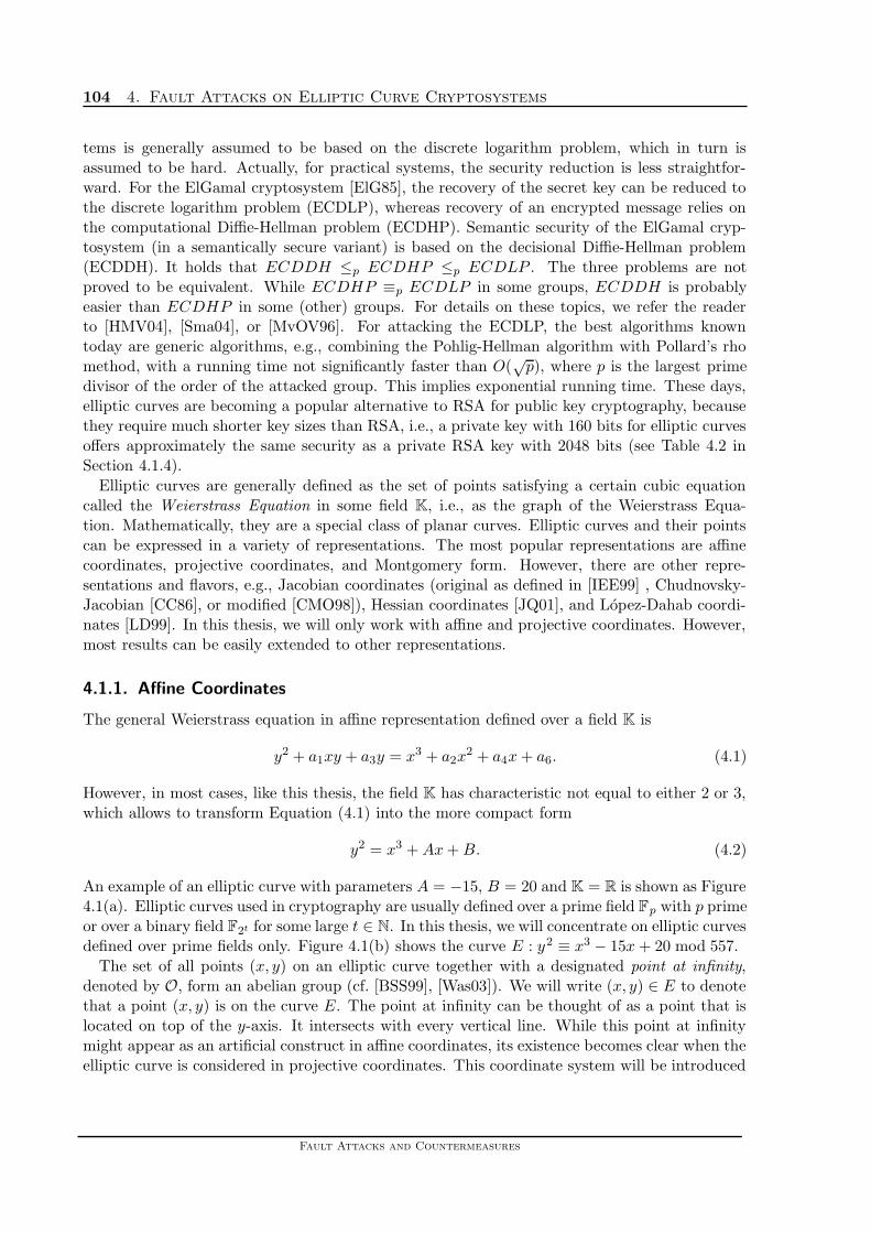
104 4. Fault Attacks on Elliptic Curve Cryptosystems
tems is generally assumed to be based on the discrete logarithm problem, which in turn isassumed to be hard. Actually, for practical systems, the security reduction is less straightfor-ward. For the ElGamal cryptosystem [ElG85], the recovery of the secret key can be reduced tothe discrete logarithm problem (ECDLP), whereas recovery of an encrypted message relies onthe computational Diffie-Hellman problem (ECDHP). Semantic security of the ElGamal cryp-tosystem (in a semantically secure variant) is based on the decisional Diffie-Hellman problem(ECDDH). It holds that ECDDH ≤p ECDHP ≤p ECDLP . The three problems are notproved to be equivalent. While ECDHP ≡p ECDLP in some groups, ECDDH is probablyeasier than ECDHP in some (other) groups. For details on these topics, we refer the readerto [HMV04], [Sma04], or [MvOV96]. For attacking the ECDLP, the best algorithms knowntoday are generic algorithms, e.g., combining the Pohlig-Hellman algorithm with Pollard’s rhomethod, with a running time not significantly faster than O(
√p), where p is the largest prime
divisor of the order of the attacked group. This implies exponential running time. These days,elliptic curves are becoming a popular alternative to RSA for public key cryptography, becausethey require much shorter key sizes than RSA, i.e., a private key with 160 bits for elliptic curvesoffers approximately the same security as a private RSA key with 2048 bits (see Table 4.2 inSection 4.1.4).
Elliptic curves are generally defined as the set of points satisfying a certain cubic equationcalled the Weierstrass Equation in some field K, i.e., as the graph of the Weierstrass Equa-tion. Mathematically, they are a special class of planar curves. Elliptic curves and their pointscan be expressed in a variety of representations. The most popular representations are affinecoordinates, projective coordinates, and Montgomery form. However, there are other repre-sentations and flavors, e.g., Jacobian coordinates (original as defined in [IEE99] , Chudnovsky-Jacobian [CC86], or modified [CMO98]), Hessian coordinates [JQ01], and Lopez-Dahab coordi-nates [LD99]. In this thesis, we will only work with affine and projective coordinates. However,most results can be easily extended to other representations.
4.1.1. Affine Coordinates
The general Weierstrass equation in affine representation defined over a field K is
y2 + a1xy + a3y = x3 + a2x2 + a4x + a6. (4.1)
However, in most cases, like this thesis, the field K has characteristic not equal to either 2 or 3,which allows to transform Equation (4.1) into the more compact form
y2 = x3 + Ax + B. (4.2)
An example of an elliptic curve with parameters A = −15, B = 20 and K = R is shown as Figure4.1(a). Elliptic curves used in cryptography are usually defined over a prime field Fp with p primeor over a binary field F2t for some large t ∈ N. In this thesis, we will concentrate on elliptic curvesdefined over prime fields only. Figure 4.1(b) shows the curve E : y2 ≡ x3 − 15x + 20 mod 557.
The set of all points (x, y) on an elliptic curve together with a designated point at infinity,denoted by O, form an abelian group (cf. [BSS99], [Was03]). We will write (x, y) ∈ E to denotethat a point (x, y) is on the curve E. The point at infinity can be thought of as a point that islocated on top of the y-axis. It intersects with every vertical line. While this point at infinitymight appear as an artificial construct in affine coordinates, its existence becomes clear when theelliptic curve is considered in projective coordinates. This coordinate system will be introduced
Fault Attacks and Countermeasures

4.1: Elliptic Curve Cryptography 105
later. O is the neutral element of the group operation, which is written in additive notationand referred to as point addition. Addition of two points on an elliptic curve is best definedgeometrically by the chord-and-tangent rule (see Figure 4.2): Given two points P1 and P2 on anelliptic curve E, the sum P3 := P1 + P2 first requires to compute −P3 as the third intersectionof E with the line defined by P1 and P2. P3 is then computed by reflecting −P3 across thex-axis. Note that if P1 = P2, the tangent line at P1 is used to determine the third intersection.If P1 = −P2, the third intersection is the point O.
5 10-5-10
10
20
30
-10
-20
-30
x
y
�P1
�P2
−(P1 + P2)�
P1 + P2�
6O
Figure 4.2.: Point addition on an elliptic curve.
Naturally, the geometric addition rule can also be expressed in a formula:
Definition 4.1 (Elliptic Curve Point Addition, Affine Coordinates).(following the IEEE P1363 standard [IEE99])Let E : y2 = x3 + Ax + B be an elliptic curve over a prime field with characteristic not equal to2 and 3. Let P1 = (x1, y1) and P2 = (x2, y2) be points on E. Then P3 := P1 + P2 is computedas follows:
1. If P1 = O, then P3 := P2, if P2 = O, then P3 := P1.
2. If P1 = −P2, i.e., if (x1, y1) = (x2,−y2), we have P3 := O.
3. If P1 6= −P2, we have P3 = (x3, y3) with
x3 := λ2 − x1 − x2 (4.3)
y3 = −y1 + λ · (x1 − x3) (4.4)
Martin Otto, Dissertation, December 2004

106 4. Fault Attacks on Elliptic Curve Cryptosystems
where λ :=
y1−y2
x1−x2if P1 6= P2
3x21+A2y1
if P1 = P2.
Note that A is the parameter from the curve equation y2 = x3 + Ax + B.
4.1.2. Projective Coordinates
Elliptic curves in projective coordinates are given by the homogeneous Weierstrass equation
E : y2z = x3 + Axz2 + Bz3, (4.5)
assuming that the underlying field K has characteristic different from 2 and 3. Points on E arerepresented as triplets P = (x : y : z). The notation of points on E arises from the fact that(x : y : z) = (λx : λy : λz) for any λ ∈ K\{0}, i.e., points are characterized by the ratio betweentheir coordinates. Here, the point at infinity is O = (0 : 1 : 0). Note that the point (0 : 0 : 0) isnot a valid point in the projective space.
Projective coordinates have a computational advantage over affine coordinates when beingdefined over a finite field. The standard addition formula requires no multiplicative inverses offield elements, which are usually expensive to compute. As the point at infinity is a valid pointin the projective space, it requires less attention than in affine coordinates. A special treatmentmay otherwise be a source for attacks, as shown in [IT03].
Jacobian and Hessian coordinates, as mentioned above, are also projective coordinates witha different weighing of the three coordinate directions.
The addition of two points P1 and P2 on E in projective coordinates is defined algorithmicallyin the following definition. A nice overview of several addition formulas for different projectivecoordinates can be found in [CMO98].
Definition 4.2 (Elliptic Curve Point Addition, Projective Coordinates).(following the IEEE P1363 standard [IEE99])Let E : y2z = x3+Axz2+Bz3 be an elliptic curve over a prime field with characteristic not equalto 2 and 3. Let P1 = (x1 : y1 : z1) and P2 = (x2 : y2 : z2) be points on E. Then P3 := P1 + P2
is defined as follows:
1. If P1 = O, then P3 = P2, if P2 = O, then P3 = P1.
2. If P1 = −P2, i.e. if (x1 : y1 : z1) = (x2 : −y2 : z2) then we have P1 + P2 = O = (0 : 1 : 0).
3. If P1 6= ±P2, then we have P1 + P2 = (x3 : y3 : z3) as
x3 :=r2 − tw2
2y3 :=vr − mw3
z3 :=z1z2w,
where u1 :=x1z22 , s1 :=y1z
32 , w :=u1 − u2, r :=s1 − s2,
u2 :=x2z21 , s2 :=y2z
31 , t :=u1 + u2, m :=s1 + s2,
and v :=tw2 − 2x3
Fault Attacks and Countermeasures

4.1: Elliptic Curve Cryptography 107
4. If P1 = P2, then we have a point doubling, 2P1 = (x3 : y3 : z3) as
x3 :=m2 − 2s
y3 :=m · (s − x3) − t
z3 :=2y1z1,
where m :=3x21 + Az4
1 , s :=4x1y21, and t :=8y4
1.
Note that A is the parameter from the projective Weierstrass Equation (4.5).
In practice, any point (x : y : z) with z = 0 is interpreted as the point O. In this case, Case 2in Definition 4.2 can be handled by Case 3, which returns z3 = 0 if P1 = −P2. Moreover, theIEEE P1363 standard [IEE99, A.10.5] suggests the following procedure: First, use the additionformula, i.e., Case 3, for all inputs. This case should return the triplet (0 : 0 : 0) if the doublingformula, i.e., Case 4, has to be applied. Then the doubling formula would be applied if necessary.
4.1.3. Elliptic Curve Cryptosystems
As elliptic curves form an abelian group, any group based cryptosystem can be based on ellipticcurves. Here, the most prominent example is the ElGamal cryptosystem. We give an examplefor EC-ElGamal in the following. It has been taken from [Cor99].
Protocol 4.3 (Elliptic Curve ElGamal Cryptosystem).System parameters: •Choose an elliptic curve E defined over a prime field Fp or over a
binary field F2t such that the order of E is divisible by a large prime q.•Choose a base point P on E of order q.
Key generation: •Choose the secret key k ∈R {1, 2, . . . , q − 1}.•Compute the public key Q = k · P on E.
Encryption: •Choose a random session key r ∈R {1, 2, . . . , q − 1}.•Compute the two points R = r · P = (x1, y1) and r · Q = (x2, y2)
(= r · k · P ).•Compute c = x2 + m, where m ∈ Zp is the message to be encrypted.• Send out (R, c) = (x1, y1, c).
Decryption •Compute (x′2, y
′2) = k · R.
•Recover m := c − x′2.
Obviously, the choice of E and P is crucial for the security of the system. The order of the basepoint P must be a large prime. Otherwise, discrete logarithm algorithms like the algorithm ofPohlig and Hellman [PH78] will be able to break the system. This implies that #E must have alarge prime factor as well. In practice, several standardization bodies recommend curves for usein cryptosystems. These curves usually have prime order or an order with a small cofactor of2 or 4, see Section 4.1.4 for details. Other security aspects, which are inherent to the ElGamalcryptosystem, must be regarded as well, e.g., no repeated use of the session key r. As they arenot motivated by the use of elliptic curves, we refer the reader to standard literature for details,e.g., [MvOV96].
We would also like to stress the point that there are many ways to embed the message m intothe system. As an alternative for the method chosen above, which simply computes an integer
Martin Otto, Dissertation, December 2004

108 4. Fault Attacks on Elliptic Curve Cryptosystems
c, it is also possible to break m into a tuple m = (m1,m2) and transmit
(R, x2 · m1, y2 · m2). (4.6)
as proposed in [GG99, §20.6]. This allows to transmit messages more efficiently. The crucialobservation is that in the case of Protocol 4.3, the y-coordinate of kR is not needed in thedecryption step, while Equation (4.6) requires the computation of the complete point kR. Thereare scalar multiplication algorithms, such as a variant of Montgomery’s binary method, which cancompute the x-coordinate only. This in turn is more efficient than computing both coordinates.However, there are verification schemes, which need the y-coordinate according to [IT02]. Notethat it is not possible to use the point M = (m, y) for some y ∈ Fp in order to embed a messagem, because it is not guaranteed that there exists a valid y-coordinate such that M is a point onE.
4.1.4. Elliptic Curve Parameters in Practice
Several standardization bodies recommend elliptic curve domain parameters. These ellipticcurves can be used in practice and they are considered to be cryptographically secure. In Table4.1, we provide an overview over the properties of these recommended curves. We consider therecommendations of IEEE P1363-2000 [IEE98], Certicom’s Standards for Efficient CryptographyGroup (SECG) [SEC00], ANSI [ANS99], Federal Information Processing Standard FIPS 186-2issued by the NIST [FIP00], the Wireless Transport Layer Security Specification by the WAPforum [WAP01], the specification for the Financial Services Markup Language (FSML) by theeCheck initiative [FSM99], the final recommendation of the NESSIE consortium [NES03], andfrom IPSec [RFC98a], [RFC98b], [IPS01].
Table 4.1 states properties of three different types of elliptic curves, curves defined over primefields Fp, curves defined over binary fields F2t and Koblitz curves. The latter refers to a specialsubset of curves which can be computed very efficiently. Koblitz curves may be defined over bothprime fields and binary fields. For binary fields, Koblitz curves usually denote special curveswith A,B ∈ {0, 1}, i.e., defined over the base field F2. A and B are the curve parameters fromthe Weierstrass equation for binary curves, which is
y2 + xy = x3 + Ax + B. (4.7)
For prime fields, Koblitz curves refer to curves which possess an efficiently computable endo-morphism. As Koblitz curves are not considered in detail in this thesis, we refer the reader to[Kob92] and [Gal99] for these details.
Elliptic curve cryptosystems offer the highest security per bit of any public key cryptosystemused today. Table 4.2 (taken from [Cer00]) presents a direct comparison of the system parametersof the same strength for RSA and elliptic curve cryptosystems.
4.2. Existing Fault Attacks on Elliptic Curve Cryptosystems
Fault attacks have first been described for the RSA cryptosystem in [BDL01]. Soon thereafter,these ideas have also been applied to several variants of elliptic curve cryptosystems. The firstsuccessful attacks aimed at special elliptic curve cryptosystems such as the KMOV cryptosystemor the Demytko cryptosystem (cf. [JQ96], [JQ97b], [JQBD97], [JLQ99]). Other attacks applied
Fault Attacks and Countermeasures
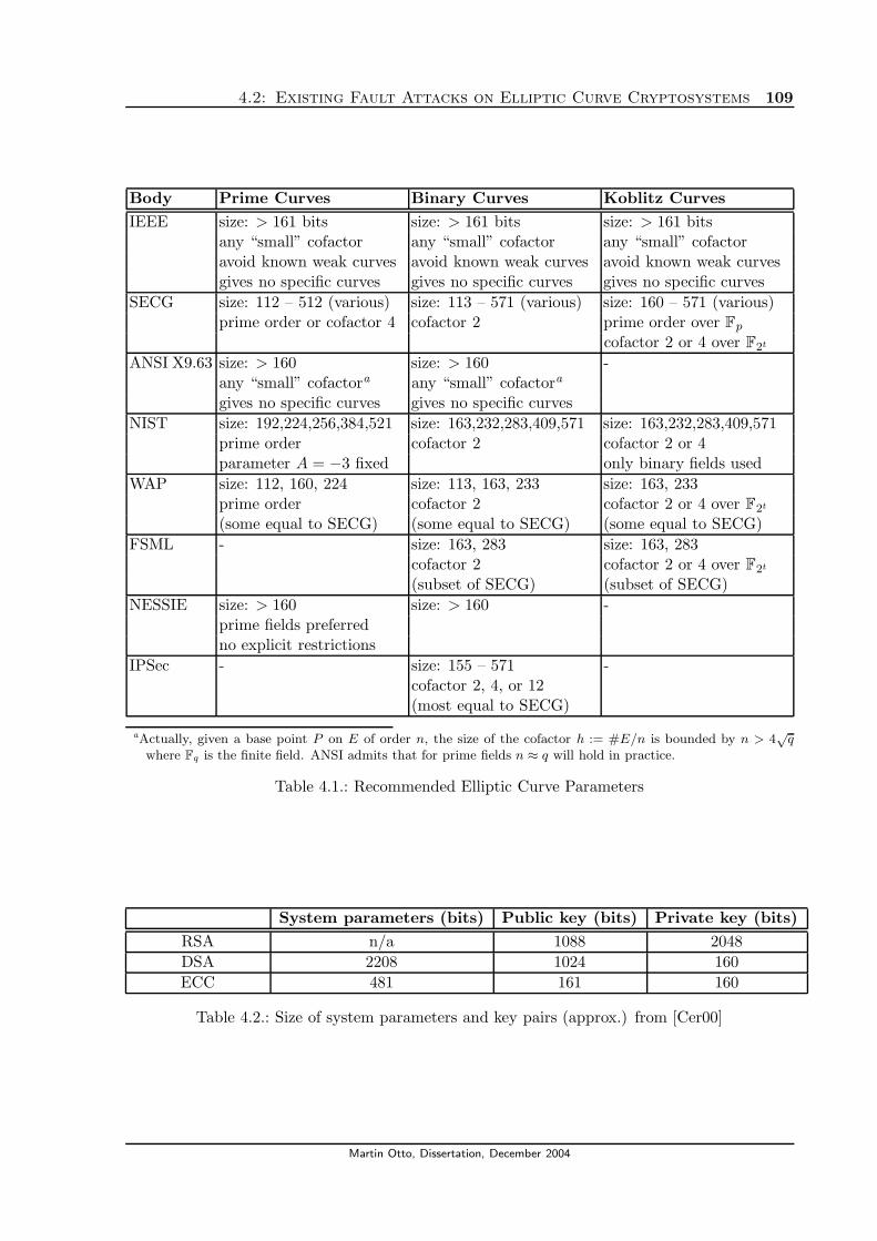
4.2: Existing Fault Attacks on Elliptic Curve Cryptosystems 109
Body Prime Curves Binary Curves Koblitz Curves
IEEE size: > 161 bits size: > 161 bits size: > 161 bitsany “small” cofactor any “small” cofactor any “small” cofactoravoid known weak curves avoid known weak curves avoid known weak curvesgives no specific curves gives no specific curves gives no specific curves
SECG size: 112 – 512 (various) size: 113 – 571 (various) size: 160 – 571 (various)prime order or cofactor 4 cofactor 2 prime order over Fp
cofactor 2 or 4 over F2t
ANSI X9.63 size: > 160 size: > 160 -any “small” cofactora any “small” cofactora
gives no specific curves gives no specific curves
NIST size: 192,224,256,384,521 size: 163,232,283,409,571 size: 163,232,283,409,571prime order cofactor 2 cofactor 2 or 4parameter A = −3 fixed only binary fields used
WAP size: 112, 160, 224 size: 113, 163, 233 size: 163, 233prime order cofactor 2 cofactor 2 or 4 over F2t
(some equal to SECG) (some equal to SECG) (some equal to SECG)
FSML - size: 163, 283 size: 163, 283cofactor 2 cofactor 2 or 4 over F2t
(subset of SECG) (subset of SECG)
NESSIE size: > 160 size: > 160 -prime fields preferredno explicit restrictions
IPSec - size: 155 – 571 -cofactor 2, 4, or 12(most equal to SECG)
aActually, given a base point P on E of order n, the size of the cofactor h := #E/n is bounded by n > 4√
qwhere Fq is the finite field. ANSI admits that for prime fields n ≈ q will hold in practice.
Table 4.1.: Recommended Elliptic Curve Parameters
System parameters (bits) Public key (bits) Private key (bits)
RSA n/a 1088 2048
DSA 2208 1024 160
ECC 481 161 160
Table 4.2.: Size of system parameters and key pairs (approx.) from [Cer00]
Martin Otto, Dissertation, December 2004

110 4. Fault Attacks on Elliptic Curve Cryptosystems
general ideas for fault attacks which worked without specific regard to elliptic curve cryptosys-tems, e.g., by attacking the pseudo random number generator used on a smartcard ([ZM96],[ZM97]), by attacking the secret scalar/exponent used in the ElGamal cryptosystem ([BDH+98],[Dot02], and [GK04]), or by using memory-safe or computational-safe errors in implementationssecure against timing or power attacks (see Section 1.6.2 and [YJ00], [YKLM01a]).
More general fault attacks exploiting specific properties of elliptic curves have been presentedin [BMM00] and [CJ03].
The attacks presented in [BMM00] target the scalar multiplication on an elliptic curve, wherethe scalar multiple Q = kP of a base point P is computed. The authors investigate what happensif the base point P is replaced by an arbitrary point P at the beginning of the multiplication.If P is not a point on the original curve E, the operation is called pseudo-multiplication, buildup by pseudo-additions. In this case, the computation of kP takes place on a different curveE. This curve is known to an adversary if P is known, which is due to the fact that the B-parameter of a curve is used neither in the addition nor in the doubling formula (see Definition4.1). Therefore, the curve E can be specified by A and a new parameter B, which can easilybe computed from the Weierstrass equation (4.2) given A and any point P . If the resultingcurve E is a cryptographically weak curve, the discrete logarithm problem might be tractable,yielding important information about the secret scalar k. Usually, several attacks are necessaryin order to recover k by combining several solutions for k modulo small primes via the ChineseRemainder Theorem.
The attack becomes feasible if an adversary can choose the base point P . This allows himto choose a cryptographically weak curve with a subgroup of small order, and a base point Pfrom such a subgroup. If the base point cannot be chosen, but it is changed by a fault attackaccording to a known fault model with a limited number of possible faulty results, e.g., the ByteFault Model 1.8, the attack is feasible as well. In this case, all possibilities for the faulty basepoint are tested until the curve E is found. If that curve allows to solve the discrete logarithmproblem, the secret scalar k can be recovered modulo some small order. The success probabilityheavily depends on the chosen fault model. The authors also extend their attack to fault attackson intermediate variables of repeated doubling, which results in a sequence of normal additionsfollowed by pseudo-additions.
In [CJ03], the results from [BMM00] are generalized. The authors show that the attack isalso feasible if random errors in either the x- or the y-coordinate are assumed, thus relaxingthe fault model to the more realistic scenario of the Random Fault Model 1.9 or the ArbitraryFault Model 1.10. With additional (strong) assumptions, even random faults in both coordinatesyield information about the secret scalar k. The attacks are also shown to be feasible for faultsinduced into the field representation, i.e., into the prime p if a prime field Fp is used or intothe irreducible polynomial used in the case of binary fields F2t. For such attacks, random faultsrequire additional knowledge to allow successful attacks, while bit or byte faults yield betterresults. For binary fields, the attack is only feasible in affine coordinates, as projective doublinguses all curve parameters. As a last generalization, Ciet and Joye show that faults induced intoany of the parameters a1, a2, a3, a4 used in the general Weierstrass Equation (4.1) can be usedfor successful attacks.
The authors of [BMM00] and [CJ03] claim that all their attacks can easily be fended off. If thesmartcard checks whether the final result is a valid point on the original curve, it is claimed thatthe check captures faulty results with an overwhelming probability. Note that this final checkrequires that all curve parameters are checked for integrity, e.g., by using CRC sums to detectpermanent errors. This result assumes that faults are induced in a way, such that the final result
Fault Attacks and Countermeasures

4.3: Undetectable Faulty Points in Point Addition 111
Q cannot be efficiently predicted and lies on the original curve only with negligible probability.In this case, the attack is not a real threat to modern systems, the proposed countermeasure iseasy and has been deployed in all modern systems today. We will refer to the countermeasureof checking if a final point is a valid point on a curve E as the standard countermeasure in thefollowing. The results from [BMM00] and [CJ03] show that elliptic curve cryptosystems aremuch more resistant against the classic fault models defined in Section 1.4 than, e.g., RSA. Thereason for this is quite simple: in RSA, any change of a value from ZN yields a valid value inZN , while in elliptic curve cryptosystems, the tuple (x, y) is characterized by a special relationbetween x and y, namely the Weierstrass Equation. Hence, faults induced into elliptic curvepoints must ensure that this condition is satisfied by the faulty values as well. There are p2 manypossible point coordinates (x, y) ∈ F2
p. However, a curve E over Fp has at most p+1+2√
p manypoints, according to Hasse’s Theorem [Sil00]. Therefore, only a very small fraction of roughly1/p of all possible point coordinates represent valid points on a specific curve. Hence, if a validpoint (x, y) is changed randomly, the chances of generating a valid point on a given curve areextremely low. Therefore, elliptic curve points are inherently more secure against fault attacksthan single finite field elements.
The crucial point in the attacks presented in [BMM00] and [CJ03] is that the authors assumethat a faulty result is not on the original elliptic curve with overwhelming probability. Suchfaulty results can be detected easily. Any attack that yields faulty results, which are valid pointson the original curve, would be undetectable by the aforementioned standard countermeasure.Such points can be used for new attacks. In the remainder of this chapter, we will carefullyderive necessary conditions for errors yielding such undetectable faulty results. We will showthat contrary to the belief in [BMM00] and [CJ03], it is possible to create undetectable errorswith a high probability, thus rendering the proposed standard countermeasure useless. This willyield a new type of fault attacks, Sign Change Faults.
4.3. Undetectable Faulty Points in Point Addition
The attacks described in Section 4.2 all worked on a “high” level of the attacked algorithms,i.e., either the scalar multiplication itself or the point or curve parameters were targeted, ratherthan the addition or doubling formulas for elliptic curve points. However, faults induced intothe addition formulas might be useful to recover secret data as well. This idea is not entirelynew. In [IT03], Izu and Takagi concentrate on the addition formulas by exploiting the fact thata projective point with zero z-coordinate cannot be transformed into affine coordinates. Anysuch point represents the point at infinity O. This raises an exception, which can yield valuableinformation if detected. However, the setting in [IT03] is rather special and it is not applicableto cryptographically secure elliptic curves. Moreover, the attack described in [IT03] does notuse faults.
Therefore, we present in the following an analysis investigating the possibility of attacks whichinduce faults into the variables used in the addition formula. We will state our results for theaffine addition formula only, because our aim is to show that undetectable faulty points can becreated. We specify what errors must be induced in order to bypass the standard countermeasuredescribed in Section 4.2. We omit an analysis of the affine doubling formula and of additionformulas for other point representations, as analyzing the affine addition already yields thedesired results. Analyses for other formulas are rather lengthy and a task best done using acomputer algebra system, e.g., Maple.
Martin Otto, Dissertation, December 2004

112 4. Fault Attacks on Elliptic Curve Cryptosystems
For our analysis, we investigate each variable used in the affine addition (see Definition 4.1(3))separately. We do not choose a specific fault model yet, as we only want to derive conditions theinflicted error has to meet in order to yield an undetectable faulty point P3. However, we mayassume that upon attack, the error induced into a variable x can be written as a summand, i.e.,x 7−→E x+ e for e ∈ Fp. We consider e to be a random variable. The distribution of e depends onthe fault model. The possibility to satisfy the conditions derived for e by any of the known faultmodels will be analyzed later. However, since some intermediate variables are used more thanonce, we will consider both transient and permanent faults. To clear notation, we introduce thefollowing definition.
Definition 4.4 (Valid Points and Valid Faulty Points).Given a point P = (x, y), we call P a valid point of the elliptic curve E if (x, y) satisfies theWeierstrass equation of E. If we investigate a certain operation, i.e., addition, doubling, orscalar multiplication, we call P a valid faulty point, if the operation has been attacked and theresulting point P is different from the correct result, yet it still satisfies the Weierstrass equationof E.
Let P1, P2 be two points on an elliptic curve E defined by its Weierstrass equation y2 ≡ x3 +Ax + B mod p. For the point addition, we assume that P1 6= ±P2. According to Definition 4.1,this implies that P3 = (x3, y3) := P1 + P2 is computed as
x3 := λ2 − x1 − x2 (4.8)
y3 = −y1 + λ · (x1 − x3) , (4.9)
where λ :=y1 − y2
x1 − x2. (4.10)
The variables used are the point coordinates x1, y1, x2, y2, the intermediate variable λ and theoutput coordinates x3 and y3. All of them can be targeted by fault attacks.
In the following, we present a small selection of results for faults induced into individualvariables as examples. The complete analysis is rather technical and has been included inthis thesis as Appendix A. It describes in detail the conditions required for an error to beundetectable. These details are given for each variable used in Equations (4.8), (4.9), and(4.10).
4.3.1. Examples for a Detailed Analysis of Undetectable Errors
In this section, we present the analyses of faults induced into two intermediate variables in detail.These results will be referred to again later in this chapter.
4.3.1.1. Faults Induced into y1 During the Computation of λ = (y1 − y2)/(x1 − x2)
For a fault induced into the variable y1 7−→E y1 + e, e ∈ Fp in Equation (4.10), we need toinvestigate both transient and permanent faults, because y1 is used again in the computation ofy3, i.e., Equation (4.9).
Transient Faults. The induced fault enforces the usage of the faulty values λ, x3, and y3 inthe computation. Given a transient fault, they take the values
λ =y1 + e − y2
x1 − x2=
y1 − y2
x1 − x2+ e = λ + e where e :=
e
x1 − x2
Fault Attacks and Countermeasures

4.3: Undetectable Faulty Points in Point Addition 113
x3 = λ2 − x1 − x2 = λ2 + 2λe + e2 − x1 − x2 = x3 + 2λe + e2
y3 = −y1 + λ (x1 − x3) = −y1 + λ(x1 − x3 − 2λe − e2
)+ e
(x1 − x3 − 2λe − e2
)
= y3 + e(x1 − x3 − 2λe − e2 − 2λ2 − λe
)= y3 + e (x1 − x3 − (e + λ) (2λ + e)) .
The resulting faulty point P3 = (x3, y3) is a valid faulty point only if it satisfies the WeierstrassEquation (4.2), i.e., if y2
3 − x33 − Ax3 − B ≡ 0 mod p. This can be used to compute e. We have
y23 − x3
3 − Ax3 − B
= e ·(
e − 2y2
x1 − x2
)·(
e2 · (x2 − x1) + 2e · (y2 − y1) +
x31 − 3x2
1x2 − Ax1 + Ax2 − 2y22 + 2x3
2 + 2y1y2
x1 − x2
)+ R,
where R = y23 − x3
3 − Ax3 − B + e · 2y1(y21 − y2
2 − x31 + x3
2 + Ax2 − Ax1)
(x1 − x2)2,
= (x2 − x1) · e ·(
e − 2y2
x1 − x2
)·(e + λ +
√2x1 + x2
)·(e + λ −
√2x1 + x2
), (4.11)
by standard arithmetic (using Maple). Here, we have R ≡ 0. This becomes evident by applyingthe Weierstrass equation, using y2
i = x3i +Axi +B for all i ∈ {1, 2, 3}. It can be applied since we
know that P1, P2, and the correct result P3 are valid points on the elliptic curve. Now, Equation(4.11) shows that we have between 2 and 4 solutions for e, since we assume that x1 6≡ x2:
e ∈{
0,2y2
x1 − x2, −λ ±
√2x1 + x2
}(4.12)
⇒ e ∈{0, 2y2, (x1 − x2) ·
(−λ ±
√2x1 + x2
)}. (4.13)
These results for e show that one transient fault which produces a valid faulty point dependson the value of y2, even if it is induced into y1. This is caused by the fact that y1 is used laterfor the computation of y3 in Equation (4.9). One might expect that negating y1 with the errore = −2y1 would yield a valid point, since the valid input point (x1,−y1) is used. However, thisdoes not yield a valid faulty point (x3, y3). For this to happen, the value y1 used in Equation(4.9) would have to be faulty as well. This requires a permanent fault, which we investigatenow.
Permanent Faults. Given a permanent fault in y1, the computations of λ and x3 are the sameas shown above for a transient fault, but the computation of y3 is different. We get the faultyoutput P3 = (x3, y3) with the values
x3 = x3 + 2λe + e2
y3 = −y1 − e + λ (x1 − x3) = y3 − e + e (x1 − x3 − e (1 + λ) (2λ + e))
= −y3 + e (x1 − x3 − e (1 + λ) (2λ + e)) − e (x1 − x2) .
As shown before, we get solutions for e by applying the Weierstrass equation (4.2), and solvingthe resulting equation for e. The computation is completely analogous to the analysis shownabove, where we describe the computation in greater detail.
Martin Otto, Dissertation, December 2004

114 4. Fault Attacks on Elliptic Curve Cryptosystems
We have
y23 − x3
3 − Ax3 − B =
(x1 − x2) · e ·(
e +2y1
x1 − x2
)·(e + λ +
√x1 + 2x2
)·(e + λ −
√x1 + 2x2
),
with standard arithmetic (using Maple). The possible solutions for e are
e ∈{0, −2y1, (x1 − x2) ·
(−λ ±
√x1 + 2x2
)}. (4.14)
As one can see in Section A.1 of Appendix A, these solutions are completely symmetric to thesolutions for an attack on y2.
4.3.1.2. Faults Induced into λ During the Computation of x3 = λ2− x1 − x2
For faults induced into λ, we investigate three different cases. First, the variable λ could havebeen affected prior to its first use in Equation (4.8). The effect of the fault could be transientor permanent. But then, it could also be that the result λ2 could have been affected. Here, wewill only analyze the case when λ is faulty, the analysis of faults affecting λ2 can be found inSection A.1 in Appendix A. In case of a fault affecting λ, the faulty value λ + e is used and weget the faulty results
x3 = (λ + e) − x1 − x2 = x3 + 2λe + e2
and y3 = −y1 + λ ·(x1 − (x3 + 2λe + e2)
)
= y3 − 2λ2e − λe2 in case of a transient fault,
or y3 = −y1 + (λ + e) ·(x1 − (x3 + 2λe + e2)
)
= y3 + e(x1 − x3 − 2λe − e2 − 2λ2 − λe
)
= y3 + e (x1 − x3 − (2λ + e) · (e + λ)) in case of a permanent fault.
Transient Faults. Let e := −2λe − e2. In this case, the resulting faulty point P3 is equal to(x3, y3) = (x3 − e, y3 +λe). In order for (x3, y3) to be a valid point on the curve, it has to satisfythe Weierstrass Equation (4.2), i.e., it must hold that
y2 ≡ x3 + Ax + B mod p.
⇒ e3 + e2(λ2 − 3x3
)+ e
(3x2
3 + A + 2y3λ)≡ 0 mod p
⇒ e ∈{
0,3x3 − λ2
2± 1
2
√λ4 − 6λ2x3 − 3x2
3 − 4A − 8y3λ
}mod p. (4.15)
As e is a quadratic equation in e, this yields 6 possible solutions for e, namely
e ∈{
0,−2λ,−λ ±√
3
2(λ2 − x3) ±
√λ4 − 6λ2x3 − 3x2
3 − 4A − 8y3λ
}mod p. (4.16)
Permanent Faults. For permanent faults affecting λ, the situation is the same as for transientfaults in y2 in the computation of λ = (y2 − y1)/(x2 − x1). It has been analyzed above yieldingthe conditions stated in Equation (4.12):
e ∈{
0,2y2
x1 − x2, −λ ±
√2x1 + x2
}
Fault Attacks and Countermeasures

4.4: Attacks Inducing Undetectable Faults 115
4.4. Attacks Inducing Undetectable Faults
In Appendix A, and with two examples in the last section, we analyze the conditions for afault on every variable used in the affine addition formula to result in a faulty output, whichcannot be detected by the standard countermeasure proposed in [BMM00] and [CJ03]. Inboth publications, [BMM00] and [CJ03], the authors suggest that their countermeasure, i.e.,checking whether the final result is a valid point on the curve E or not, is sufficient as acountermeasure against fault attacks on elliptic curves. In this section, we will show that thisclaim is wrong. By inducing faults into coordinate values during a point addition, it is possibleto create undetectable errors yielding valid faulty points. We will show that these attackshave a very high success probability. Therefore, the countermeasure proposed in [BMM00] and[CJ03] is rendered useless by these attacks. Moreover, this countermeasure actually supportsour new attacks by eliminating all other faulty results, which do not represent valid faultypoints. This allows attacks to be less precise. Once again, a countermeasure against one attackactually benefits another, a situation first described in [YKLM01a]. As noted before, we referto the countermeasure of checking if a final point is a valid point on a curve E as the standardcountermeasure.
Let x be the faulty variable changed by the adversary using some specific fault model. Theeffect of the fault can be expressed by the mapping
x 7−→E x = x + e(x), (4.17)
where e(x) represents the error compared to the correct value x. The possible values for e(x)are determined by the fault model used. First, we show that using random faults, the standardcountermeasure is indeed sufficient. Afterwards, we will investigate bit faults and byte faultsand show that these faults lead to a new fault type, Sign Change Faults, which is not thwartedby the standard countermeasure.
4.4.1. Faults Induced into Point Addition Using Random Faults
First, we consider the Random Fault Model defined in Definition 1.9. Here, we interpret theerror term e(x) from Equation (4.17) as a random variable, which is uniformly distributed in theinterval {−x,−x+1, . . . , 2l(p)−1−x}. This interval is derived from the fact that x ∈ {0, 2l(p)−1}.All computations are performed within the finite field Fp, hence, we may treat e(x) as a randomvariable from the interval {−x,−x + 1, . . . , 2l(p) − 1 − x} mod p = {0, 1, . . . , p − 1} = Fp. Theerror e(x) is not a uniformly distributed variable in Fp because 2l(p) is not a multiple of p. Valuesof e(x) smaller than 0 or larger than p − 1 are wrapped around by the reduction. However, asp < 2l(p) ≤ 2p, each value in Fp has at most two preimages in {−x,−x + 1, . . . , 2l(x) − 1 − x}.Therefore, we have Prob(e(x) ≡ c mod p) ∈ {1/p, 2/p}. There is a bias in the distributiontowards the boundary values, however, given the fact that p is a large prime, the differencebetween 1/p and 2/p is negligible.
For all variables analyzed in the last section, an error has to satisfy a certain condition. Givenfixed points P1 and P2 on a fixed curve E, an error has to take at least one out of at most 6different values in Fp in order to allow an undetectable fault. For example, a transient faultinduced into the intermediate variable λ during the computation of x3, results in a valid faultypoint iff
e ∈{
0,−2λ,−λ ±√
3
2(λ2 − x3) ±
√λ4 − 6λ2x3 − 3x2
3 − 4A − 8y3λ
}mod p,
Martin Otto, Dissertation, December 2004

116 4. Fault Attacks on Elliptic Curve Cryptosystems
according to Equation (4.16). Here, the condition e = 0 is not an option for an adversary, as itreturns the correct result. Therefore, for any targeted variable, the success probability to inducean undetectable fault is at most 5/p, which is negligible. Attacks using the random fault modelin the above described manner are useless for an adversary.
4.4.2. Faults Induced into Point Addition Using Bit Faults
Now, we consider the Single Bit Fault Model as defined in Definition 1.7. A fault induced intoa variable x is assumed to result in an error e(x) = ±2b mod p for some 0 ≤ b ≤ l(p) − 1.Therefore, such bit faults represent a very small number of possible errors. The Single Bit FaultModel generally neglects the fact that bits can only be flipped to the complementary value, i.e.,only one out of the the two error values e = 2b and e = −2b is actually possible. However, thisdetail is usually not important in practice. Thus the total number of different faulty values forx is at most 2l(p). As l(p) ≈ log(p), an adversary can check all possible errors by exhaustivesearch. This is the main advantage of bit errors compared to random errors as mentioned beforein Section 1.4.2.
In the case of an error occurring in the addition routine, the task is to show that some of theconditions for the induced error e can be met using bit flips.
Judged by the complexity of the conditions for the error e, some of the conditions look easierto accomplish. The important cases are the following error conditions:
• e = −2y2 (transient error in y1 in the computation of λ, see Equation (4.13)), or
• e = −2y1 (permanent error in y1 in the computation of λ, see Equation (4.14)), or
• e = −2λ (transient error in λ in the computation of x3, see Equation (4.16)),
or as shown in Appendix A,
• e = −2y2 (error in y2 in the computation of λ, see Equation (A.3)),
• e = −2y3 (error in y1 in the computation of y3, see Equation (A.10)), or
• e = −2y3 (error in y3 in the computation of y3, see Equation (A.11)).
In the situation where the corresponding coordinate or value is a power of 2, these conditions canbe met by a bit flip. For example, if P1 = (x1, y2) and P2 = (x2, y2) should be added to P1 + P2
where y2 = 2b, and the 2b+1st bit of y1 is 0, a bit flip of that bit in y1 during the computationof λ yields a valid faulty point according to Equation (4.13) (see first condition above). If anadversary is able to choose the base point P in a scalar multiplication, he might be able tocompute a point P such that at some step kP +k ′P is computed where the above conditions aremet. For a concrete example, consider the standard left-to-right repeated doubling algorithmfor scalar multiplication on elliptic curves, presented as Algorithm 4.5 on the next page.
If an adversary can choose a base point P = (x2, y2) such that y2 = 2b for some 0 ≤ b < l(p)−1,a bit flip fault can be induced in each execution of Line 4 in Algorithm 4.5. If the error e = 2b+1
is induced into the y-coordinate of Q during the computation of the slope λ, Algorithm 4.5computes Q := Q−P , which is a valid faulty result. For bit flips, we usually assume that any bitof a variable is hit with the same uniform probability, hence, after a small number of attempts,an adversary can hope to induce the desired fault. Moreover, the standard countermeasureactually helps in this attack. It will sort out all those faulty values, which do not satisfy any
Fault Attacks and Countermeasures

4.5: Sign Change Faults 117
of the error conditions derived in Section 4.4. Therefore, an adversary can induce faults untila faulty value is returned by the device. In this case, the adversary knows exactly how thisfaulty result has been created. This enables him to successfully recover the secret scalar k, givenenough faulty values. This attack will be described in the next chapter. Note that the otherfault types described in Section 1.3 can also be used for this attack. Additionally, it is obviousthat the Chosen Bit Fault Model, Definition 1.6 can be used for this attack as well, with an evengreater success probability.
Algorithm 4.5: Left-to-right Repeated Doubling on an Elliptic Curve E
Input: A point P on E, and a secret key 1 < k < ord(P), where n denotes the binary length ofk, i.e. the number of bits of k
Output: kP on E# init1 Set Q := O# main2 For i from n − 1 down to 0 do3 Set Q := 2Q4 If di = 1 then set Q := Q + P5 Output Q
The fault type which is described here follows a certain pattern. It changes the sign of a variable.If the value y2 is changed to y2 − 2y2, the point used is P2 = −P2 = (x2,−y2). It is obviouslya valid point, yet, it does not yield the correct result. This type of error always circumventsthe standard countermeasure. We will therefore introduce it as a new fault type, Sign ChangeFaults. These are described in the following. We have shown that this fault type can be realizedusing bit faults if the base point P has a special y-coordinate. We will show in the following thatSign Change Faults can also be realized in several other ways, which shows that this fault typeis realistic. In the following chapters, we will use this fault type to successfully attack ellipticcurve scalar multiplication.
4.5. Sign Change Faults
In this section, we describe a new fault type, Sign Change Faults. We show how Sign ChangeFaults can be induced into physical devices, thus showing that the new model is practical.Attacks using this new fault model will be presented in the next chapter. This new fault typehas been published as [BOS04].
Definition 4.6 (Fault Type: Sign Change Fault Type).Let X be a variable affected by a Sign Change Fault (SCF). Then the variable is changed to thefixed value
X 7−→E X = −X.
Neither the value of X nor of X is known to the adversary. The effect of the fault may betransient or permanent.
Sign changes can be applied to any variable in any cryptosystem. However, due to the differentnature of sign changes, such attacks show very different success probabilities in practice. Fora point P = (x, y) on an elliptic curve E(Fp), where p > 3 is prime, a sign change is just a
Martin Otto, Dissertation, December 2004

118 4. Fault Attacks on Elliptic Curve Cryptosystems
change of the sign of the y-coordinate, i.e., P 7−→E (x,−y). However, if the point P is a pointon an elliptic curve E(F2t) for some t, a sign change can be expressed as P 7−→E (x, x − y). Thisobviously requires a much more aggressive change of the bits of the y-coordinate. For values xin ZN , where N = p · q with p, q prime as in the RSA cryptosystem, sign changes have a verysimilar effect as for points P over prime fields, p 7−→E − p = N − p mod N .
At first sight, a Sign Change Fault does not seem to be easily performed in a general setting.A random change of the y-coordinate cannot hope to yield −y with non-negligible probabilityas shown in Section 4.4.1. However, there exist several special yet common settings, whereSign Change Faults can be realized. From the above considerations, it seems that changing they-coordinate of an elliptic curve point defined over a prime field is easier than changing a pointdefined over a binary field. This is indeed true, most examples for a successful induction of SignChange Faults only apply to elliptic curves defined over prime fields. In the following, we willintroduce possible attacks, which yield faults of the Sign Change Fault type. These results havebeen achieved in cooperation with Johannes Blomer and Jean-Pierre Seifert [BOS04].
Symmetric Representation. One possible scenario assumes that an implementation of finitefield arithmetic works with positive and negative field elements. This implementation could storethe sign of such a field element as a single bit together with the absolute value. In this case,attacks on that single bit are possible with a variety of fault models. As the minimal amountof memory which can be allocated by a smartcard is one byte, all fault models assuming faultsin a single bit, a byte or in all bits using any fault type as defined in Section 1.3 can be used tochange the sign bit. However, there are some slight drawbacks: First, attacking a byte in orderto flip the least significant bit, the sign bit, is not always successful in every fault model, e.g.,random faults have a success probability of 1/2. Second, a smartcard could easily check if thevalue of the sign byte is greater than 1 and trigger a security reset if this is the case. This wouldlower the success probability to 1/256, if all byte values are equally probable. Therefore, bytefaults and random faults have a lower success probability, although still acceptably high.
Usually, finite field elements are not stored with an explicit sign bit, since they can be easilyrepresented by the canonical set {0, 1, . . . , p − 1}, given a modulus p. However, it is possibleto use a symmetric representation with the set {−(p − 1)/2, . . . ,−1, 0, 1, . . . , (p − 1)/2}. Herenumbers can be represented using one bit less, which might give a small advantage in speed asnegation of elliptic curve points is very cheap. In this case, the sign bit is used and Sign ChangeFaults are possible. Unfortunately, a symmetric number system is hardly used in practice.
NAF-based Elliptic Curve Scalar Multiplication. The performance of most variants of theclassical repeated doubling algorithm will improve if the scalar k is recoded into non-adjacentform (NAF). The 2-NAF uses digits from the set {−1, 0, 1} and ensures that no two adjacentdigits are non-zero. It achieves a higher ratio of zeros to non-zeros, which reduces the numberof additions/subtractions in the resulting double-and-add-or-subtract method. For details onthe NAF, see [Boo51], [Rei60], [Mac61], [Hwa79], [Kor93], [JY00], [Ott01], or [OT04]. Usingthe NAF, subtractions are introduced. Since negating a point on an elliptic curve simply meansto change the sign of the y-coordinate, subtractions are extremely cheap operations on ellipticcurves. They require at most an additional subtraction, i.e., −x = p − x, where p is themodulus. The savings using repeated doubling based on the NAF are 11.11% on average (see[MO90]), because the NAF has an expected 33% lower Hamming-weight than the correspondingbinary expansion and it is at most one bit longer than the binary expansion. It can be createdfrom the binary expansion or any other signed digit representation with the same digit set
Fault Attacks and Countermeasures

4.5: Sign Change Faults 119
in linear time (cf. [Ott01]). Other variants using a signed m-ary digit set {−(m − 1),−(m −2), . . . ,−1, 0, 1, . . . ,m − 1} exist, which also yield significant savings [OT04], [Ott01]. Becauseof these improvements, NAF based variants of repeated doubling are often used in modernsmartcards. Any of these NAF based variants of the repeated doubling algorithm is susceptibleto Sign Change Faults.
The most direct attack on the NAF is to induce a SCF in one of the signed digits of therecoded scalar k. This means to change a digit from −1 to +1 or vice versa, whereas a 0 is notchanged at all. Although there exist compact representations of signed-digit representations, cf.[JT01a], the most popular encoding described in [JY00] admits a straightforward bit-flip attack.Note that an attacker being able to induce faults according to the Chosen Bit Fault Model 1.6has no difficulties to induce the formerly sketched SCF on the recoded k.
Another conceivable way to attack the NAF is offered by the fact that any NAF-based algo-rithm has to incorporate a conditional branch, where for any secret key bit ki = 1 an additionis performed and for any secret key bit ki = −1, a subtraction is performed. Currently, a wholezoo of physical attacks is available to either target the bit ki (see Section 1.1) or to targetthe conditional decision itself (e.g., power spikes or clock glitches as described in Section 1.1).These attacks aim at forcing the conditional statement to choose the wrong branch. In case of aNAF-based version of Algorithm 4.5 (which will be described later as Algorithm 5.2), choosingthe wrong branch means to add −P instead of P or vice versa. This results in a transientSign Change Fault induced into the point P . This attack is also valid for more sophisticatedNAF-based repeated doubling variants, which aim to secure the basic scheme against power andtiming attacks, e.g., by using dummy operations (cf. [Cor99]).
Attacks On The Crypto Co-Processor. Besides attacking the scalar multiplication algorithmon a high level, Sign Change Faults can also be realized by attacking the addition and multi-plication procedures, which are used to compute point coordinates. One practical scenario forthis attack relies on the internal functionality of many real-world embedded crypto co-processorssupporting modular arithmetic, cf. [HP98] and [BOPV03]. Namely, in order to speed up thetime-critical modular multiplication operation, they most often also rely on the non-adjacentform, cf. [Boo51], [Mac61], and [Kor93]. For practicability issues most often only the classical2-NAF recoding is used. However, this time, it is not the secret scalar k, which is transformedinto NAF, but factors used during the computation of P1 + P2 for two elliptic curve points P1
and P2 (see below). Therefore, this attack also applies to variants of the repeated doublingalgorithm, which are not based on the NAF of the secret scalar multiplier k.
The crucial point that we are exploiting here is that any efficient implementation of the NAFmust provide special hardware to handle negative numbers, i.e., being able to compute the 2th
complement of any register used as a multiplicand without time delay. Actually, considering theprototypical architecture of such an embedded crypto co-processor, cf. [BOPV03] and [Sed87],this task is trivial to solve. Namely, simply invert every bit send to the long integer arithmeticunit (ALU) and additionally add +1. Note that providing this functionality is a must forthe modulus register in order to implement the underlying modular multiplication algorithmefficiently, cf. [Mon85], [Sed87], [WQ90], [Bar96] or [BOPV03]. For concreteness we refer to[Sed87] and its corresponding patent [Sed89]. Other prominent embedded real-world cryptoco-processors with similar characteristics are described in [HP98] and [BOPV03]. Given thisfunctionality, it can be used for an attack.
We consider such a crypto co-processor, cf. [Sed87], adding simultaneously at least threedifferent operands with a possible sign change in one single instruction. Changing the value of
Martin Otto, Dissertation, December 2004

120 4. Fault Attacks on Elliptic Curve Cryptosystems
an operand to its negative, i.e., to its 2th complement, one usually needs to change only one singlebit among the control signals of the corresponding ALU. This is due to the fact that the ALUof most crypto co-processors is, as already explained above, designed to handle automaticallythe 2th complement of any operand. Here, an attack can be mounted that results in an SCF.
Let us now examine the addition formulas in greater detail to see which Sign Change Faultsyield valid faulty points.
Affine Addition. Let us recall the affine addition formula, Definition 4.1, for two points P1 =(x1, y1) and P2 = (x2, y2), both not equal to O:
x3 := λ2 − x1 − x2
y3 = −y1 + λ · (x1 − x3) ,
where λ :=
y1−y2
x1−x2. if P1 6= ±P2
3x21+A2y1
if P1 = P2.
These formulas show that lots of load/store and exchange operations are needed in the ALUin order to compute the desired result (x3, y3). Therefore, attacks on the crypto co-processorduring these operations may change the control signals, thus negating the loaded value. If,for example, the value y1 is changed to −y1 in the computation of λ, a valid faulty point P3 iscreated according to Equation (4.14). Any variable used in the formulas must be loaded into theALU at some time before the computation can be performed. During this preparing load/storeor exchange instruction, the corresponding value must go through the ALU. While executingthis operation, the handled value is susceptible to an SCF as only a single bit among the controlsignals must be changed to load/store or exchange the value in its target register to its negative.This yields an SCF by changing one single control signal. Note that [BCN+04] actually describeshow to implement such physical attacks in practice.
A sign change in a variable x can be described as x 7−→E x = x + e, where e = −2x. Wehave seen four examples in Section 4.4.2, where sign changes in variables used in the affineaddition formula yield valid faulty points. Two simple possibilities are described in SectionA.1 in Appendix A: First, we could change the sign of y2 in the computation of y1 − y2 whilecomputing λ, according to Equation (A.3). Second, we could change the sign of y3 after thecorrect result has been computed according to Equation (A.11). The two other possibilitiesdepend on the implementation. According to Equation (4.14), a permanent sign change of thevalue y1 prior to its first use also yields a valid faulty point. However, a permanent fault canonly be achieved by an attack on the ALU if the value y1 is only loaded/stored once, i.e., if thefaulty value is used for all occurrences in the addition formula. The last possibility is a faultinduced into the value λ used to compute x3. According to Equation (4.16), a transient faultinduced into λ will yield a valid faulty point P3. However, in order to achieve a transient faultin λ, this value would have to be computed or loaded twice, such that the value used in thecomputation of y3 is correct again. This is highly unlikely in an efficient implementation.
For the affine doubling, similar considerations apply. Obviously, any sign change in variablesused in the computation of x3 and y3 yield the same result as for the affine addition. However,the computation of λ is different. Here, it is clear that any permanent change of y1 yields a validfaulty point P3. Whether a permanent fault can be induced depends on the implementation.
Fault Attacks and Countermeasures

4.5: Sign Change Faults 121
Projective Addition. Sign Change Faults via the ALU can also be induced into the projectiveaddition formula, which has been presented in Definition 4.2. This is easy to see. Let P1 =(x1 : y1 : z1), P2 = (x2 : y2 : z2) be elliptic curve points in projective coordinates. For a pointaddition, we have
x3 :=r2 − tw2 2y3 :=vr − mw3 z3 :=z1z2w,
where u1 :=x1z22 , s1 :=y1z
32 , w :=u1 − u2, r :=s1 − s2,
u2 :=x2z21 , s2 :=y2z
31 , t :=u1 + u2, m :=s1 + s2,
and v :=tw2 − 2x3
and for doubling the point P1 = (x1 : y1 : z1):
x3 :=m2 − 2s y3 :=m · (s − x3) − t z3 :=2y1z1,
where m :=3x21 + Az4
1 , s :=4x1y21 , and t :=8y4
1 .
Again, it becomes clear that lots of load/store or exchange instructions are needed in order torealize this formulas involving the coordinates of the original points P1 and P2. For example,an implementation could use y1 or y2 via previous load/store or exchange instructions as amultiplicand in the modular multiplications to compute s0, s1, z3, or t.
Concluding Remarks. All attack settings introduced above can be further relaxed, taking intoaccount that the device will check whether the final output is a valid point on the curve or notto defend against the attacks described in Section 4.2. In this case, faults which change singlebits with an acceptably high probability, e.g., byte faults according to Fault Model 1.8, can beused, because unsuccessful physical attacks are winnowed by this final check.
Some of the attacks described above can be applied to curves defined over both, prime fieldsand binary fields. This is true for attacks on a symmetric representation and on the NAF, asattacks here do not initiate a finite field negation, but indicate that a point negation must beperformed. For an attack on the crypto co-processor, however, the faulty control signal triggersa field negation, which yields a negated point only in the case of prime field based elliptic curves.For binary field based elliptic curves, a point is negated by replacing the y-coordinate by x− y.Hence, this is different from −y unless we are in the special case where x = 0.
The above considerations show that Sign Change Faults can be induced in a large varietyof settings, most of which represent today’s modern smartcard environments. Therefore, SignChange Faults are practical. They fulfill the condition stated in Chapter 1, demanding thatfault models and fault types must be justified in practice in order to be a valuable subject ofanalysis. In the next chapter, we will show how Sign Change Faults can be used to successfullyrecover a secret scalar factor k.
Martin Otto, Dissertation, December 2004

122 4. Fault Attacks on Elliptic Curve Cryptosystems
Fault Attacks and Countermeasures

5. Sign Change Faults — Attacking EllipticCurve Cryptosystems
The results of Section 4.4.1 show that elliptic curve cryptosystems are easy to secure againstmost classic fault types, e.g., random faults. However, we have shown that a new fault type, SignChange Faults, represents a practical and thus dangerous attack on elliptic curve cryptosystems.Here, faulty values, which are undetectable by the standard countermeasure described in Section4.2, can be created with a very high chance of success. In this section, we will show how to useSign Change Faults to break elliptic curve cryptosystems.
In all cryptosystems based on elliptic curves, e.g., the ElGamal cryptosystem and its variants,a crucial computation is the scalar multiplication of a public base point P with a secret scalarfactor k. Attacks aim to recover the value k. In this chapter, we show how Sign ChangeFaults can be used to successfully attack a variety of implementations of elliptic curve scalarmultiplication, namely the NAF-based left-to-right repeated doubling in Section 5.1, the NAF-based right-to-left repeated doubling in Section 5.2, the classic repeated doubling in Section5.3, and Montgomery’s binary method in Section 5.4. The attacks succeed to recover the secretscalar factor efficiently.
Sign Change Attacks will be the main topic of the remainder of this thesis. The next chapter,Chapter 6, is devoted to the presentation and analysis of a new countermeasure, which protectsscalar multiplication algorithms against Sign Change Attacks. Chapter 7 will briefly show thatSign Change Faults can also be applied successfully to modular exponentiation, i.e., in thecontext of the RSA cryptosystem.
First, we need to define our fault model, which is based on the Sign Change Fault type:
Definition 5.1 (Fault Model: Sign Change Faults / (sc) fault model).We have defined a Sign Change Fault (SCF) as the flipping of the sign of a given variable inDefinition 4.6. Sign Change Faults are defined both for elliptic curve points as well as for finitefield elements:
x 7−→E − x mod p for x ∈ Fp
P 7−→E − P for P a point on some elliptic curve E
where
P = (x, y) 7−→E − P = (x,−y) P affine point on E defined over a prime field
P = (x, y, z) 7−→E − P = (x,−y, z) P projective point on E defined over a prime field
We define the Sign Change Fault Model, (sc) fault model, with the following parameters.
123

124 5. Sign Change Faults — Attacking Elliptic Curve Cryptosystems
location: complete control (can target the sign of a specific variable)timing: no control (cannot target a specific point of time, every operation and every
iteration of a loop, where the targeted variable is involved, is hit with thesame (uniform) probability)
number of bits: random number of faulty bits (the sign is changed)fault type: Sign Change Faults (see Definition 4.6)probability: certain (every physical attack results in a fault of the desired kind)duration: permanent faults and transient faults (both variants are investigated if they
differ, however, it is assumed that an adversary cannot use both kinds inone attack setting)
5.1. Sign Change Attack on NAF-based Left-to-Right RepeatedDoubling
We first present an attack on the NAF-based left-to-right repeated doubling algorithm, becausethis is the most important example of repeated doubling in practice. The left-to-right methodis preferred over the right-to-left version, because it does not need an additional variable. Asdiscussed in Section 2.2, there are attacks on repeated doubling algorithms, which show thatit is not self-evident that an attack on one version carries over seamlessly to the other version,e.g., [FV03]. Hence, we will present both results in this thesis.
Since negating an elliptic curve point is a very cheap operation, practical applications usuallyuse a NAF-based repeated doubling algorithm. Therefore, we put our main focus on NAF-basedvariants as well. We have described the NAF in some detail in Section 4.5.Sign Changes do not depend on the underlying representation of the elliptic curve points, i.e.,they apply to affine and projective coordinates as well. All of our attacks apply to both repre-sentations alike, hence, we will not assume a special representation in this chapter.
In Algorithm 5.2, we present a NAF-based left-to-right version of the well known repeateddoubling algorithm. Algorithm 5.2 already implements the standard countermeasure againstrandom fault attacks from Section 4.2 in Line 5.
Algorithm 5.2: NAF-based Repeated Doubling on an Elliptic Curve E (Left-to-Right Version)
Input: A point P on E, and a secret key 1 < k < ord(P) in non-adjacent form, where n denotesthe number of bits of k
Output: kP on E# init1 Set Q := O
# main
2 For i from n − 1 downto 0 do3 Set Q := 2Q4 If ki = 1 then set Q := Q + P else if ki = −1 then set Q := Q − P5 If Q is not on E then set Q := O6 Output Q
Starting from Algorithm 5.2, we will use indices to distinguish between the variable values inthe main loop. We will denote the correct final result by Q and a faulty final result by Q. Toavoid ambiguity when referring to intermediate values, we rewrite Lines 3 and 4 as
Fault Attacks and Countermeasures

5.1: Sign Change Attack on NAF-based Left-to-Right Repeated Doubling 125
3 Set Q′i := 2Qi+1
4 If ki = 1 then set Qi := Q′i + P
If ki = 1 else if ki = −1 then set Qi := Q′i − P
If ki = 1 else if ki = −1 else set Qi := Q′i
Naturally, we set Qn := O.Most elliptic curves defined over prime fields, which are recommended by current standards
such as ANSI, IEEE, and SECG (see Table 4.1), have prime order, i.e., they contain a primenumber of points. Therefore, we will assume this property for our curves as well. This factimplies that any point P 6= O on E must have the same (large) prime order. We will use thisassumption frequently.
We state our attack using an algorithm similar to the attack presented by Boneh, DeMilloand Lipton in [BDL01] on RSA. This attack has been analyzed and used extensively in Chapter2. Similar to [BDL01], we need to be able to induce faults into c = (n/m) log(2n) runs on thesame input (P, k,E) to recover k with probability at least 1/2. Here, m is a parameter to bedefined later. Differently from the attack in [BDL01], we need a correct result Q to verify ourtest cases — which is indeed a plausible assumption. We use the following result from [BDL01]to bound the number of necessary faulty outputs needed by our attack (see also Fact 2.4).
Fact 5.3 (Number of Necessary Attacks).Let x = (x1, x2, . . . , xn) ∈ {0, 1}n and let M be the set of all contiguous intervals of length m < nin x. If c = (n/m) · log(2n) bits of x are chosen uniformly independently at random, then theprobability that each interval in M contains at least one chosen bit is at least 1/2.
5.1.1. Sign Change Attack Targeting Q′
iin Line 4.
All of the variables in Lines 3 and 4 can be successfully targeted by a Sign Change Attack (SCA).In the following, we present a fault attack, which induces faults into the variable Q ′
i in Line 4during some loop iteration n−1 ≥ i ≥ 0. Afterwards, we will describe how to modify the attackfor the other variables.
The basic idea of our attack algorithm is to recover the bits of k in pieces of 1 ≤ r ≤ m bits.Here, m is chosen to reflect a trade-off between the number of necessary faulty results derivedfrom Fact 5.3 and the approximate amount 2m of offline work. Throughout this chapter, weassume that 2m � #E. To motivate the algorithm, we first assume that a faulty value Q isgiven that resulted from an SCF in Q′
i. In order to describe the resulting pattern in a compactway, we introduce the following notation, similar to Definition 2.17.
Definition 5.4 (High and Low Parts of k and kP ).Let (kn−1, kn−2, . . . , k0) be the binary expansion or NAF of a positive integer k and let P be apoint on an elliptic curve. We define upper and lower parts of k and kP as
hi(k) :=n−1∑
j=i
kj2j−i, Hi(k) := hi(k) · P, (5.1)
li(k) :=i∑
j=0
kj2j , Li(k) := li(k) · P. (5.2)
In the context of scalar multiplication, k denotes the secret scalar factor. If the number k isclear from the context, we will write hi for hi(k) etc.
Martin Otto, Dissertation, December 2004

126 5. Sign Change Faults — Attacking Elliptic Curve Cryptosystems
Corollary 5.5 (Transformations Between Li And Hi).Let k and P be defined as in Definition 5.4. With Q :=
∑n−1j=0 kj2
jP , we have the followingequalities:
Li(k) = Q − 2i+1Hi+1(k) (5.3)
Hi(k) =Q − Li−1(k)
2i(5.4)
Proof:
We have
Q − 2i+1Hi+1(k) =
n−1∑
j=0
kj2jP − 2i+1
n−1∑
j=i+1
kj2j−i−1P =
i∑
j=0
kj2jP = Li(k).
This proves Equation (5.3), which directly yields Li−1(k) = Q − 2iHi(k). This in turnimplies Equation (5.4). �
Equation (5.4) uses division, which is not explicitly defined for elliptic curves. However, weassume elliptic curves defined over fields with prime order, therefore, since 2i 6≡ 0 mod #E,multiplicative inverses are guaranteed to exist. Hence, division is just multiplication with themultiplicative inverse as usual. This justifies the above notation. Moreover, the right hand sideof Equation (5.4) adds up the summands kj2
j with j ≥ i. Therefore, every summand is divisibleby 2i, hence, a multiplicative inverse is not needed if instead the summands kj2
j−i are used.In a correct run of Algorithm 5.2, the final value Q = Q0 = kP is computed as
Q = 2 · (2 · (. . . 2 · (2 · (2 · (kn−1P ) + kn−2P ) + kn−3P ) . . .) + k1P ) + k0P
= 2 ·(. . . 2 ·
(2 ·(Q′
i + kiP)
+ ki−1P). . .)
+ k0P with Q′i =
n−1∑
j=i+1
kj2j−iP
(5.1)= 2Hi+1(k)
= 2iQ′i +
i∑
j=0
kj2jP
(5.1),(5.2)= 2i+1Hi+1(k) + Li(k).
Now it is easy to see that a faulty value Q, which results from a fault induced into Q′i, can be
written as:
Q = −2iQ′i +
i∑
j=0
kj · 2j · P = −2in−1∑
j=i+1
kj2j−iP +
i∑
j=0
kj · 2j · P
(5.2)= −Q + 2Li(k) (5.5)
(5.3)= Q − 2 · 2i+1Hi+1(k). (5.6)
On the right hand side of Equation (5.5), the only unknown part is Li(k), which defines amultiple of P . If only a small number of the signed bits k0, k1, . . . , ki used in that sum isunknown, these bits can be guessed and verified using Equation (5.5). This allows to recover thesigned bits of k starting from the LSBs. Moreover, based on Equation (5.6) it is also possible torecover the signed bits of k starting from the MSBs (see Section 5.1.3). As we assume that faults
Fault Attacks and Countermeasures

5.1: Sign Change Attack on NAF-based Left-to-Right Repeated Doubling 127
are induced uniformly at random, an adversary may choose freely between these two recoverystrategies. In the following, we will use the LSB version based on Equation (5.5). We assumethat Q is known. The complete attack is stated as the following algorithm.
Algorithm 5.6: The Sign Change Attack on Q′i
Input: Access to Algorithm 5.2, n the length of the secret key k > 0 in non-adjacent form, Q = kPthe correct result, m a parameter for acceptable amount of offline work.
Output: k with probability at least 1/2.# Phase 1: Collect Faulty Outputs1 Set c := (n/m) · log(2n)2 Create c faulty outputs of Algorithm 5.2 by inducing a SCF in Q′
i for random values of i.
3 Collect the set S = {Q | Q 6= Q is a faulty output of Algorithm 5.2 on input P}.# Phase 2: Inductive Retrieval of Secret Key Bits4 Set s := −1 indicating the number s + 1 of known bits of k.5 While (s < n − 1) do
# Compute the known LSB part 2Ls(k) of the exponent k.6 Set L := 2
∑sj=0 kj2
jP
# Try all possible bit patterns with length r ≤ m.7 For all lengths r = 1, 2, . . . m do8 For all valid NAF-patterns x = (xs+1, xs+2, . . . , xs+r) with xs+r 6= 0 do
# Compute the test candidate Tx
9 Set Tx := L + 2∑s+r
j=s+1 xj2jP
# Verification Step: Verify the test candidate using Equation (5.5)
10 for all Q ∈ S do
11 if(Tx − Q
)= Q then
12 conclude that ks+1 = xs+1, ks+2 = xs+2, . . . , ks+r = xs+r,13 set s := s + r, and continue at Line 5# Handle a Zero Block Failure14 If no test candidate satisfies the verification step, then15 assume that ks+1 = 0 and set s := s + 1.16 Verify Q = kP. If this fails then output FAILURE.17 Output k
Comment. Algorithm 5.6 has been abbreviated for clarity in two minor details. On the onehand, the highest iteration that suffered a SCF in Line 2 of Algorithm 5.6 needs not be the lastiteration n−1. Let j be the maximal i such that the value Q′
i has been attacked. Algorithm 5.6only recovers bits of k up to iteration j. Following Fact 5.3, we assume a “lucky case”, whichmeans that we assume that every interval of length m was targeted by at least one SCF. Thisonly guarantees that j ≥ n − m. Hence, the m − 1 most significant bits may not be recovered.However, up to m − 1 missing bits can easily be recovered by exhaustive search if m is smallenough. If this fails, the adversary comes to the same conclusion as suggested in Line 16: theguessed bits must be wrong and the attack has failed.
Furthermore, it is clear that given n as the length of the NAF of k, Algorithm 5.6 does notneed to test patterns whenever s + r ≥ n. Here, s indicates that the s + 1 least significant bitsk0, k1, . . . , ks are known. In fact, we may assume that the most significant bit of k is kn−1 = 1,otherwise n cannot be uniquely defined. Therefore, we may assume w.l.o.g. that s + r < n − 1.
Martin Otto, Dissertation, December 2004

128 5. Sign Change Faults — Attacking Elliptic Curve Cryptosystems
Note that we always have k > 0. We also rely on the fact that (k0, k1, . . . , ks, xs+1, . . . , xs+r)(constructed in Line 8) is always in valid NAF.
We will prove the success of Algorithm 5.6 in two lemmas. First, we will show that only acorrect guess for the pattern of k can satisfy the verification step in Line 11. Then, we will showthat Algorithm 5.6 will always correctly recover at least the next unknown bit of k. The secondresult is based on the assumption that each contiguous interval of m bits was targeted by atleast one Sign Change Fault. This represents the “lucky case” of Fact 5.3. Before stating theresults, we introduce Zero Block Failures. This definition is essentially the same as Definition2.8, but here we put it in the context of Sign Change Faults on elliptic curve points.
Definition 5.7 (Zero Block Failure).Assume that Algorithm 5.6 already recovered the s+1 least significant signed bits k0, k1, . . . , ks ofk. If the signed bits ks+1, ks+2, . . . , ks+r are all zero and all Sign Change Faults that happenedin iterations s + 1, . . . , s + m are restricted to the first r iterations s + 1, s + 2, . . . , s + r, thesituation is called a Zero Block Failure.
We briefly recall the notion of Zero Block Failures, which was introduced before in the contextof RSA in Section 2.1.2. A Zero Block Failure is named after the fact that errors in a blockof zeros will not be detected as errors within that block. Equation (5.2) shows that for anys, Ls(k) = Ls+1(k) = . . . = Ls+r(k) for all sequences ks+1 = 0, ks+2 = 0, . . . , ks+r = 0. Inthis case, the values Q1 = −Q + 2Ls(k) and Q2 = −Q + 2Ls+r(k) are equal. Therefore, givenQ = −Q + 2Ls(k), Algorithm 5.6 cannot determine how many zero bits — if any — follow ks.Hence, tailing zeros must be neglected, because their number cannot be determined correctly.This is the reason why Algorithm 5.6 only tests patterns x which end in ±1 in Line 8. However,the fact that tailing zeros do not change the value of Q allows us to write Q = −Q+2Li(k) withki 6= 0 for some unknown i if Q 6= −Q. Moreover, if it is known that Q = −Q+ 2Ls(k), we mayspecify i in greater detail. In fact, we have Q = −Q+2Li(k) with i := max{j | kj 6= 0 ∧ j ≤ s}.The case where Q = −Q, i.e., when the maximum does not exist, can be represented by choosingi = −1. This simplification will be used in the following two lemmas.
First, we will investigate the case when a test pattern x satisfies the verification step. Thisallows Algorithm 5.6 to recover the next r bits of k.
Lemma 5.8 (No False Positives).If Algorithm 5.6 computes a test bit pattern x such that Tx satisfies the verification step in Line11 for some Q ∈ S, then x is the correct bit pattern.
Proof:
Assume that the verification step is satisfied for a given test bit pattern x = (xs+1, . . . , xs+r)with 1 ≤ r ≤ m and xs+r 6= 0, x in non-adjacent form. We assume that we have afalse positive, i.e., the pattern x is different from the corresponding pattern of k, namelyks+1, ks+2, . . . , ks+r. Hence, there must be a faulty result Q ∈ S that satisfies the ver-ification step in Line 11 together with this x. The verification step in Line 11 yieldsO = Tx − Q − Q. We use Line 9 of Algorithm 5.6 to express Tx and Equation (5.5) toexpress Q in detail. As explained above, we may assume that Q = −Q + 2Li(k) withki 6= 0 for some unknown i ≥ 0. We have
O =
2 ·
s∑
j=0
kj2jP + 2 ·
s+r∑
j=s+1
xj2jP
−
−Q + 2 ·
i∑
j=0
kj2jP
− Q
Fault Attacks and Countermeasures

5.1: Sign Change Attack on NAF-based Left-to-Right Repeated Doubling 129
= 2 ·
s∑
j=0
kj2j +
s+r∑
j=s+1
xj2j
︸ ︷︷ ︸R+
−i∑
j=0
kj2j
︸ ︷︷ ︸R−
· P = Rx · P (5.7)
where Rx = 2 ·max(i,s+r)∑
j=0
yj2j and yj =
0 if j ≤ min(i, s)kj if i < j ≤ s(xj − kj) if s < j ≤ min(i, s + r)xj if max(i, s) < j ≤ s + r−kj if s + r < j ≤ i.
Equation (5.7) implies that either Rx = 0 or Rx is a multiple of the order of P .
Case 1. Assume that Rx = 0. This is easily shown to be impossible. It implies thatR+ = R−, i.e., both sums are valid NAF representations of the same number. Since theNAF is unique, this implies that both representations are equal. Hence, all digits are equalin contradiction to the assumption that there is as least one xj 6= kj with s+1 ≤ j ≤ s+r.
Case 2. Assume that Rx 6= 0 is a multiple of the order of P on E. We know thatord(P ) = #E � 2m as #E is prime. Therefore, #E divides Rx. If i = −1, i.e., Q = −Q,we have Rx · P = Tx = O. As we may assume that s + r < n − 1 as explained above,we have Rx < #E. This contradicts our assumption that #E divides Rx. If 0 ≤ i ≤ s,we have Rx = 2i+2 · R′
x with |R′x| < 2s+r−i < 2n−1−i ≤ k < #E. Therefore, #E
cannot divide Rx. If s + 1 ≤ i ≤ s + r, we have Rx = 2s+2 · R′x with |R′
x| < 2m+1.Again, #E cannot divide Rx. For s + r < i < n − 1, we have Rx = 2s+2 · R′
x with|R′
x| < 2i−s+1 ≤ 2n−2−s+1 ≤ 2n−1 ≤ k < #E. Therefore, #E cannot divide Rx. The lastcase, i = n − 1, is impossible. It would imply that Q′
i = O has been attacked, where noSign Change Fault can be induced, i.e., Q = Q. However, we explicitely prevent valuesQ = Q from being members of the set S in Line 3 of Algorithm 5.6. Therefore, Case 2 isimpossible. �
Lemma 5.7 has shown that if Algorithm 5.6 has found a test pattern x, it correctly representsthe corresponding bit pattern of k. This result can be used to show that whether Algorithm 5.6finds a test pattern x or not, it always recovers the correct next bits of k.
Lemma 5.9 (Correct Recovery).We assume that the bits k0, k1, . . . , ks of k have already been computed by Algorithm 5.6. Fur-thermore, we assume that a Sign Change Fault was induced into the intermediate value Q ′
i inLine 4 of Algorithm 5.2 for some i ∈ {s + 1, s + 2, . . . , s + m}.
Then, in order to recover the next signed bit ks+1, Algorithm 5.6 will be in one of two cases:In the first case, it finds a test bit pattern x = (xs+1, xs+2, . . . , xs+r), r ≤ m, that satisfies theverification step in Line 11 and concludes that kj = xj for all s + 1 ≤ j ≤ s + r in Line 12. Inthe second case, it detects a Zero Block Failure and concludes that ks+1 = 0 in Line 15. In bothcases, the conclusion is correct and between 1 and r bits of k are recovered correctly.
Proof:
We will investigate the two cases of the lemma separately.
Martin Otto, Dissertation, December 2004

130 5. Sign Change Faults — Attacking Elliptic Curve Cryptosystems
Case 1. Assume that Algorithm 5.6 finds a test bit pattern x = (xs+1, xs+2, . . . , xs+r)that satisfies the verification step in Line 11. According to Lemma 5.8, there cannot bea false positive and x correctly represents the bit pattern of k. Therefore, the conclusionkj = xj for all s + 1 ≤ j ≤ s + r is correct.
Case 2. Assume that Algorithm 5.6 does not find a test bit pattern x that satisfies theverification step. In this case, a Zero Block Failure is conjectured by Algorithm 5.6 and itsets ks+1 = 0.
We assume that this conjecture is wrong. We know by the assumption in the lemma thatat least one of the iterations s + 1, s + 2, . . . , s + m was targeted by a Sign Change Fault.Let Q ∈ S be the faulty output resulting from such an induced fault, i.e., Q = −Q+2Li(k)with s + 1 ≤ i ≤ s + m according to Equation (5.5). If the conjecture that we have aZero Block Failure is wrong, we know by Definition 5.7 that we may choose Q such thatat least one of the bits ks+1, ks+2, . . . , ki is not zero. This implies that we may writeQ = −Q + 2Lw(k) with w := max{j | kj 6= 0 ∧ s + 1 ≤ j ≤ i} as explained above.Now it is easy to see that the test bit pattern 0 6= x = (ks+1, ks+2, . . . , kw−1, kw) of length1 ≤ r ≤ m satisfies the verification step. This means that the value Tx defined in Line 9of Algorithm 5.6 correctly represents 2Lw(k). Therefore, a valid test pattern x exists andAlgorithm 5.6 will find a value for ks+1 in Line 12. Hence, the assumption that a ZeroBlock Failure is detected incorrectly must be wrong. �
The results of the previous lemmas are summarized in the following theorem. It is a straight-forward result from the two previous lemmas, combined with a simple count of the operationsperformed by Algorithm 5.6.
Theorem 5.10 (Success of the Proposed Sign Change Attack).Algorithm 5.6 succeeds to recover the secret scalar multiple k of bit length n in time O(n·2m ·c·M)with probability at least 1/2. Here, c = (n/m) · log(2n) and M is the maximal cost of a full scalarmultiplication or a scalar multiplication including the induction of a Sign Change Fault.
Proof:
The result of Lemma 5.9 relies on the assumption that every contiguous interval of lengthm was targeted by at least one Sign Change Fault in Line 2 of Algorithm 5.6. Accordingto Fact 5.3, this assumption holds with probability 1/2 if c = (n/m) · log(2n) faulty resultsare collected. This requires c scalar multiplications with the ability to induce a SCF.According to Lemma 5.9, every iteration of the while loop of Algorithm 5.6 recovers eithera zero bit or a test bit pattern x. It shows that this recovery is always correct if the “luckycase” of Fact 5.3 is assumed. Therefore, Algorithm 5.6 recovers between 1 and m bits ineach while iteration. Therefore, at most n iterations are needed. The worst case occurswhen k = 2n−1 and no SCF was induced into Q′
n−1 while Algorithm 5.6 created the setof faulty outputs in Line 2. As all bits but the most significant are zero, only Zero BlockFailures would occur, allowing to recover only a single bit in each iteration of Algorithm5.6.
In a single iteration, Algorithm 5.6 first computes the value L in Line 6, requiring a singlescalar multiplication. Then, the algorithm tests at most all possible NAF patterns of
Fault Attacks and Countermeasures

5.1: Sign Change Attack on NAF-based Left-to-Right Repeated Doubling 131
length m (assuming tailing zeros for shorter patterns). These are at most
η =1
3·(2m+2 + (−1)m+1
)= O(2m),
according to [EK90]. Every test bit pattern x yields a test candidate Tx using one scalarmultiplication in Line 9. Obviously, some speedups could be applied, e.g., storing Tx allowsto compute a new Tx using a single addition. Note that the precomputation of L in Line 6already represents a speed up. For each test candidate Tx, at most c point additions andcomparisons need to be done in Line 11. If all possible bits of k have been recovered, alast full scalar multiplication must be applied to differentiate between Zero Block Failuresand a real failure. This yields total costs of
O(c · M + n · (M + 2m · c · (A + C)) + M),
where M denotes the cost of a full scalar multiplication, M the cost of a full scalarmultiplication with the ability to induce a fault, A the cost of a point addition, and C thecost of a point comparison. To present a short result, we simply treat the addition andcomparison cost of Line 11 together as one full scalar multiplication. We also assume thatM = M .
In this case, the worst case running time of Algorithm 5.6 is O((c + n2mc + 1) ·M) wherec = (n/m) · log(2n) and M is the maximal cost of a full scalar multiplication or a scalarmultiplication including the induction of a Sign Change Fault. �
5.1.2. Other Attacks
The basic idea of Algorithm 5.6 can also be used for Sign Change Attacks, which induce faultsinto any other variable used inside the loop in Algorithm 5.2. We have explicitly investigatedan attack targeting the variable Q′
i in Line 4 of Algorithm 5.2 in the previous section. However,if the variable Q′
i in Line 3 is affected by an induced fault, it has the exact same effect. For theother variables, we will briefly present the results in the following.
Attacks targeting Qi+1 in Line 3. A fault induced into Qi+1 in Line 3 changes the sign ofQi+1. This yields Q′
i = 2 · (−Qi+1) = −Q′i, which is the same error as if Q′
i would be affectedby a fault induced into Line 3 or 4. Hence, all results from the previous section apply.
A fault induced into the variable Qi+1 in Line 3 of Algorithm 5.2 can be used for another SignChange Attack if it is possible to target just one of the two copies of Qi+1. In this case, a SignChange Fault induced into Qi+1 yields Q′
i = O and
Q = Li(k).
Algorithm 5.6 can be used to recover the bits of k starting from the LSBs with the followingmodified verification step:
11(a) if(2Q − Tx
)= O then
This attack does not need to know a correct result Q. We can prove that this verificationstep does not yield any false positives with Lemma 5.8. The proof is completely analogous withopposite signs in Equation (5.7). Lemma 5.9 and Theorem 5.10 hold unchanged. With Equation(5.3), we get Li(k) = Q − 2i+1Hi+1(k). Hence, it is also possible to recover the bits starting
Martin Otto, Dissertation, December 2004

132 5. Sign Change Faults — Attacking Elliptic Curve Cryptosystems
from the MSBs.
Attacks targeting the Base Point P in Line 4. Another attack can be mounted if it is possibleto change the sign of the base point P in Line 4. Since the base point is used in every iteration,we need to differentiate between a transient fault, where only once a faulty value −P is used,and a permanent fault, which changes all subsequent usages of P as well.
If the error induced into P is transient, we have
Q = Q − 2ki2iP.
Algorithm 5.6 can be used if the verification step is modified to
11(b) if(Q + 2xs+12
s+1P)
= Q then
Obviously, changing only the modification step here means to break a butterfly on a wheel, aswe may save a lot of operations since neither L nor Tx are needed. If ki = 0, this fault has noeffect. If ki = ±1, we have a single bit changed, which is essentially the same as a sign change ofthe bit ki of the secret scalar. A drawback of this attack is that we need a block size of m = 1,hence, an increased number of faulty outputs need to be collected. In addition, a lot of ZeroBlock Failures will occur, as every zero in the NAF of k yields a Zero Block Failure. The resultof Lemma 5.8 about the impossibility of false positives holds for this special case as well, simplyassume that all bits besides ki and xs+r are equal to zero in Equation (5.7) and change thesigns of R+ and R−. Hence, Theorem 5.10 holds for this case as well, showing that the attacksucceeds to recover k in polynomial time.
If the error induced into P is permanent, we have
Q = Q − 2Li(k).
Algorithm 5.6 can also be used for this case with only a sign change in the verification step, i.e.,
11(c) if(Q + Tx
)= Q then
Obviously, the two lemmas and the theorem of Section 5.1 hold as well.
Attacks targeting P should be considered much less probable than attacks targeting any othervariable. As P is the base point, it is stored in long term memory, where it is loaded from everytime. Moreover, permanent errors could easily be detected by re-checking.
An Attack targeting Qi in Line 4. A fault induced into Qi in Line 4 yields Q = 2Li−1(k)−Q.This yields the exact same attack as described in Algorithm 5.6.
5.1.3. Recovering The Bits Starting From The MSB
As mentioned above, the bits of k can also be recovered starting from the MSB, based onEquation (5.6), which states that
Q = Q − 2 · 2i+1Hi+1(k).
Algorithm 5.6 has to be modified accordingly, yet, the claims about the success probability holdfor this attack as well, with some modifications. For completeness, we present the modifiedalgorithm here. The modified parts have been highlighted. Note that we assume that kn−1 = 1.
Fault Attacks and Countermeasures
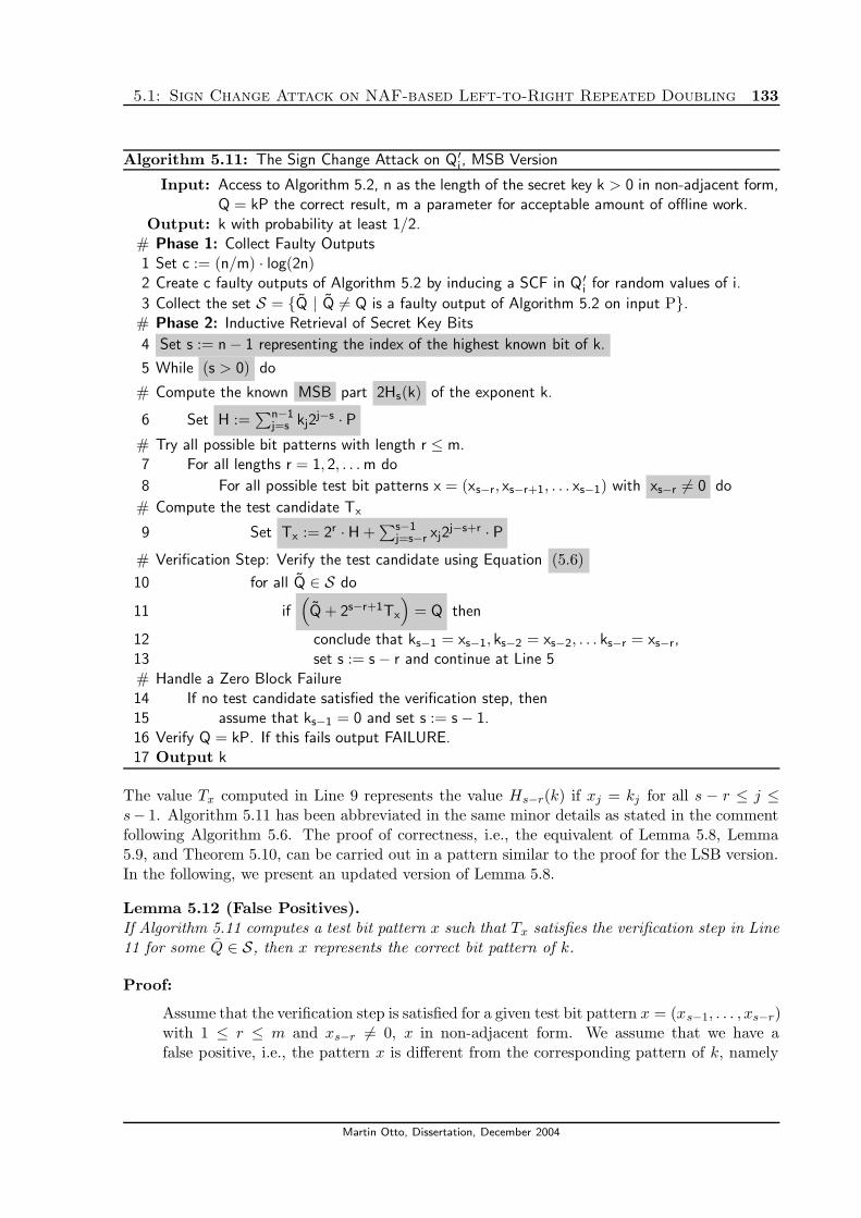
5.1: Sign Change Attack on NAF-based Left-to-Right Repeated Doubling 133
Algorithm 5.11: The Sign Change Attack on Q′i, MSB Version
Input: Access to Algorithm 5.2, n as the length of the secret key k > 0 in non-adjacent form,Q = kP the correct result, m a parameter for acceptable amount of offline work.
Output: k with probability at least 1/2.# Phase 1: Collect Faulty Outputs1 Set c := (n/m) · log(2n)2 Create c faulty outputs of Algorithm 5.2 by inducing a SCF in Q′
i for random values of i.
3 Collect the set S = {Q | Q 6= Q is a faulty output of Algorithm 5.2 on input P}.# Phase 2: Inductive Retrieval of Secret Key Bits
4 Set s := n − 1 representing the index of the highest known bit of k.
5 While (s > 0) do
# Compute the known MSB part 2Hs(k) of the exponent k.
6 Set H :=∑n−1
j=s kj2j−s · P
# Try all possible bit patterns with length r ≤ m.7 For all lengths r = 1, 2, . . . m do
8 For all possible test bit patterns x = (xs−r, xs−r+1, . . . xs−1) with xs−r 6= 0 do
# Compute the test candidate Tx
9 Set Tx := 2r · H +∑s−1
j=s−r xj2j−s+r · P
# Verification Step: Verify the test candidate using Equation (5.6)
10 for all Q ∈ S do
11 if(Q + 2s−r+1Tx
)= Q then
12 conclude that ks−1 = xs−1, ks−2 = xs−2, . . . ks−r = xs−r,13 set s := s − r and continue at Line 5
# Handle a Zero Block Failure14 If no test candidate satisfied the verification step, then15 assume that ks−1 = 0 and set s := s − 1.16 Verify Q = kP. If this fails output FAILURE.17 Output k
The value Tx computed in Line 9 represents the value Hs−r(k) if xj = kj for all s − r ≤ j ≤s− 1. Algorithm 5.11 has been abbreviated in the same minor details as stated in the commentfollowing Algorithm 5.6. The proof of correctness, i.e., the equivalent of Lemma 5.8, Lemma5.9, and Theorem 5.10, can be carried out in a pattern similar to the proof for the LSB version.In the following, we present an updated version of Lemma 5.8.
Lemma 5.12 (False Positives).If Algorithm 5.11 computes a test bit pattern x such that Tx satisfies the verification step in Line11 for some Q ∈ S, then x represents the correct bit pattern of k.
Proof:
Assume that the verification step is satisfied for a given test bit pattern x = (xs−1, . . . , xs−r)with 1 ≤ r ≤ m and xs−r 6= 0, x in non-adjacent form. We assume that we have afalse positive, i.e., the pattern x is different from the corresponding pattern of k, namely
Martin Otto, Dissertation, December 2004
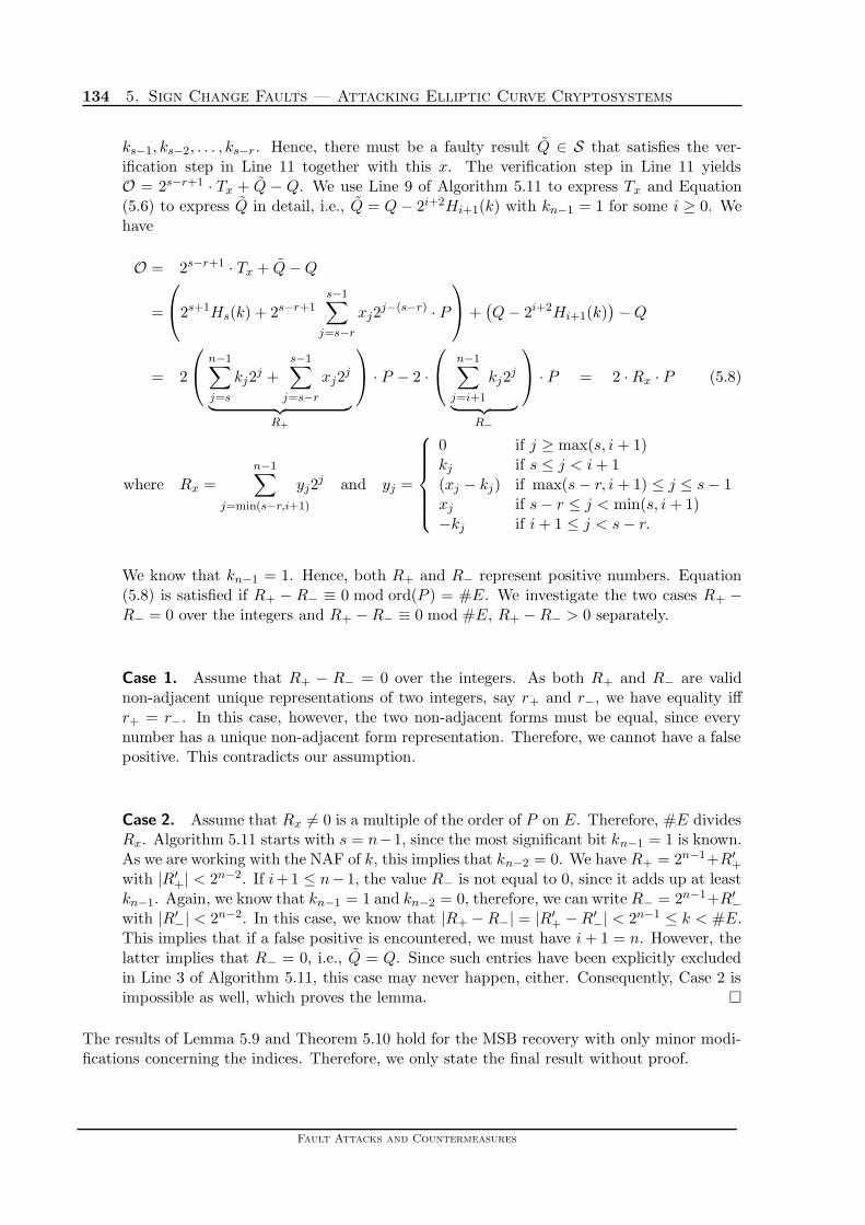
134 5. Sign Change Faults — Attacking Elliptic Curve Cryptosystems
ks−1, ks−2, . . . , ks−r. Hence, there must be a faulty result Q ∈ S that satisfies the ver-ification step in Line 11 together with this x. The verification step in Line 11 yieldsO = 2s−r+1 · Tx + Q − Q. We use Line 9 of Algorithm 5.11 to express Tx and Equation(5.6) to express Q in detail, i.e., Q = Q − 2i+2Hi+1(k) with kn−1 = 1 for some i ≥ 0. Wehave
O = 2s−r+1 · Tx + Q − Q
=
2s+1Hs(k) + 2s−r+1
s−1∑
j=s−r
xj2j−(s−r) · P
+
(Q − 2i+2Hi+1(k)
)− Q
= 2
n−1∑
j=s
kj2j +
s−1∑
j=s−r
xj2j
︸ ︷︷ ︸R+
· P − 2 ·
n−1∑
j=i+1
kj2j
︸ ︷︷ ︸R−
· P = 2 · Rx · P (5.8)
where Rx =
n−1∑
j=min(s−r,i+1)
yj2j and yj =
0 if j ≥ max(s, i + 1)kj if s ≤ j < i + 1(xj − kj) if max(s − r, i + 1) ≤ j ≤ s − 1xj if s − r ≤ j < min(s, i + 1)−kj if i + 1 ≤ j < s − r.
We know that kn−1 = 1. Hence, both R+ and R− represent positive numbers. Equation(5.8) is satisfied if R+ − R− ≡ 0 mod ord(P ) = #E. We investigate the two cases R+ −R− = 0 over the integers and R+ − R− ≡ 0 mod #E, R+ − R− > 0 separately.
Case 1. Assume that R+ − R− = 0 over the integers. As both R+ and R− are validnon-adjacent unique representations of two integers, say r+ and r−, we have equality iffr+ = r−. In this case, however, the two non-adjacent forms must be equal, since everynumber has a unique non-adjacent form representation. Therefore, we cannot have a falsepositive. This contradicts our assumption.
Case 2. Assume that Rx 6= 0 is a multiple of the order of P on E. Therefore, #E dividesRx. Algorithm 5.11 starts with s = n−1, since the most significant bit kn−1 = 1 is known.As we are working with the NAF of k, this implies that kn−2 = 0. We have R+ = 2n−1+R′
+
with |R′+| < 2n−2. If i+1 ≤ n− 1, the value R− is not equal to 0, since it adds up at least
kn−1. Again, we know that kn−1 = 1 and kn−2 = 0, therefore, we can write R− = 2n−1+R′−
with |R′−| < 2n−2. In this case, we know that |R+ − R−| = |R′
+ − R′−| < 2n−1 ≤ k < #E.
This implies that if a false positive is encountered, we must have i + 1 = n. However, thelatter implies that R− = 0, i.e., Q = Q. Since such entries have been explicitly excludedin Line 3 of Algorithm 5.11, this case may never happen, either. Consequently, Case 2 isimpossible as well, which proves the lemma. �
The results of Lemma 5.9 and Theorem 5.10 hold for the MSB recovery with only minor modi-fications concerning the indices. Therefore, we only state the final result without proof.
Fault Attacks and Countermeasures

5.2: Sign Change Attack on NAF-based Right-to-Left Repeated Doubling 135
Theorem 5.13 (Success of the Proposed Sign Change Attack).Algorithm 5.11 succeeds to recover the secret scalar multiple k of bit length n in time O(n·2m·c·M)with probability at least 1/2. Here, c = (n/m) · log(2n) and M is the maximal cost of a full scalarmultiplication or a scalar multiplication including the induction of a Sign Change Fault.
5.2. Sign Change Attack on NAF-based Right-to-Left Repeated
Doubling
As we have explained above, attacks on one version of repeated doubling are not guaranteed toapply to other variants of repeated doubling as well in general. Therefore, we will investigate inthis section, how a Sign Change Attack can be mounted on the twin of the left-to-right repeateddoubling algorithm (Algorithm 5.2): the right-to-left repeated doubling algorithm. We will seethat for Sign Change Attacks, both versions are susceptible for these attacks in the same manner.We start with stating the right-to-left repeated doubling algorithm as Algorithm 5.14.
Algorithm 5.14: NAF-based Repeated Doubling on an Elliptic Curve E (Right-to-Left Version)
Input: A point P on E, and a secret key 1 < k < ord(P) in non-adjacent form, where n denotesthe number of bits of k
Output: kP on E# init1 Set Q := O2 Set R := P# main3 For i from 0 to n − 1 do4 If ki = 1 then set Q := Q + R else if ki = −1 then set Q := Q − R5 Set R := 2R6 If Q is not on E then set Q := O7 Output Q
We will investigate Sign Change Attacks against Algorithm 5.14 in the same manner as in Section5.1.1. Again, we will use indices to differentiate between the variable values in the main loop.We denote the correct final result by Q and a faulty final result by Q. To refer to intermediatevalues clearly, we rewrite Lines 4 and 5 as
4 If ki = 1 then set Qi := Qi−1 + Ri−1
If ki = 1 else if ki = −1 then set Qi := Qi−1 − Ri−1
If ki = 1 else if ki = −1 else set Qi := Qi−1
5 Set Ri := 2Ri−1
5.2.1. Sign Change Attack Targeting Qi in Line 4.
In a correct run of Algorithm 5.14, the final value Q = Qn−1 = kP is computed as
Q = k020 · P + k12
1 · P + . . . + kn−12n−1 · P
=(
k020 · P + k12
1 · P + . . . + ki2i · P︸ ︷︷ ︸
=Qi=Li(k)
)+ ki+12
i+1 · P + . . . + kn−12n−1 · P
Martin Otto, Dissertation, December 2004

136 5. Sign Change Faults — Attacking Elliptic Curve Cryptosystems
= Qi + ki+12i+1 · P + . . . + kn−12
n−1 · P (5.1),(5.2)= Li(k) + 2i+1Hi+1(k).
Now it is easy to see that a faulty value Q, which results from an attack inducing a SCF in Qi,can be written as:
Q = −Qi + 2i+1Hi+1(k) = −Li(k) + 2i+1Hi+1(k)
(5.2)= Q − 2Li(k) (5.9)
(5.3)= −Q + 2 · 2i+1Hi+1(k). (5.10)
Equations (5.9) and (5.10) allow to recover the bits of k starting from the LSBs or startingfrom the MSBs. They are the same formulas as Equation (5.5) and (5.6) for the attack on theleft-to-right version, only with the opposite sign. Let us first assume that we wish to recoverthe bits of k starting from the LSBs, i.e., using Equation (5.9). In this case, the Sign ChangeAttack targeting Qi in the right-to-left repeated doubling algorithm is completely analogous toAlgorithm 5.6. The only difference is a new verification step, that respects the opposite sign.The modified Line 11 simply replaces Tx − Q be Tx + Q, i.e.,
11(d) if(Tx + Q
)= Q then
Not surprisingly, the analysis of this modified attack is completely equivalent to the analysisof the original Algorithm 5.6. The results of Lemma 5.8 (no false positives), of Lemma 5.9(correct recovery), and of Theorem 5.10 (success probability and runtime) carry over seamlessly,even the proofs change only negligibly. Therefore, we omit the lemmas and the proofs here andstate the final result only.
Theorem 5.15 (Success of the Proposed Sign Change Attack).Algorithm 5.6 with the modified verification step
11(d) if(Tx + Q
)= Q then
succeeds to recover the secret scalar multiple k of bit length n in time O(n · 2m · c · M) withprobability at least 1/2. Here, c = (n/m) · log(2n) and M is the maximal cost of a full scalarmultiplication or a scalar multiplication including the induction of a Sign Change Fault.
5.2.2. Other Attacks
The basic idea of Algorithm 5.6 can also be used for Sign Change Attacks inducing faults intoany other variable used inside the loop in Algorithm 5.14. Once again, we state the results forall variables individually.
An Attack targeting Qi−1 in Line 4. A fault induced into Qi−1 in Line 4 yields Q = Q −2Li−1(k), hence, Algorithm 5.6 can also be used for this case with the same modification stepas in Theorem 5.15.
Attacks targeting Ri−1 and Ri in Lines 4 and 5. The variable values of Ri−1 and Ri areused twice, once for the computation of Qi and once for the computation of Ri (or Qi+1 andRi+1, respectively). Therefore, faults induced into Ri−1 in Line 4 or Ri in Line 5 are differentdepending on whether the induced fault is a transient fault or a permanent fault. Since a fault
Fault Attacks and Countermeasures

5.2: Sign Change Attack on NAF-based Right-to-Left Repeated Doubling 137
in Ri has the same effect as a fault in Ri−1, just in a different iteration of the loop, we do notneed to consider both scenarios separately. We will only investigate attacks targeting Ri−1.
Transient Faults. In case of a transient fault induced into Ri−1 in Line 4, the intermediatevalue Qi is changed to Qi = Qi−1 − kiRi−1 = Qi − 2kiRi−1. Since we assume a transient fault,the correct value for Ri−1 is used when the value Ri is computed in Line 5. Therefore, theremaining computation is correct, and we get
Q = Qi − 2kiRi−1 +
n−1∑
j=i+1
kj2jP = Q − 2kiRi−1 = Q − 2i+1ki · P, since Ri = 2i+1P.
Therefore, Algorithm 5.6 can be used with a modified verification step
11(e) if(Q + xs+12
s+2P)
= Q then
However, a larger number of faulty values must be collected as these Sign Change Faultsrequire a block length of m = 1. For bit values ki = 0, the attack has no effect, for other bitvalues it represents a bit flip of the secret scalar factor k. This case represents the same situationas an attack on the base point P in Line 4 of Algorithm 5.2, which has been described in greaterdetail in Section 5.1.2.
A transient fault induced into Ri−1 in Line 5 has the same effect as a permanent fault inducedinto Ri in Line 5. This is due to the fact that Ri−1 is no longer used after Line 5 and the valueRi = 2Ri−1 is computed with a wrong value, i.e., Ri = 2 · (−Ri−1) = −Ri.
Permanent Faults. In Line 4 of Algorithm 5.14, the variable Ri−1 takes the value Ri−1 = 2iP .If it is affected by an induced fault, the value changes to Ri−1 = −2iP , so subsequent values ofR also have their sign changed if the change is permanent. We assume that the fault changesthe sign of Ri−1 before it is used to create Qi. Ultimately, the faulty final result Q will be
Q = Qi−1 −n−1∑
j=i
kj2jP = −Q + 2Qi−1 = −Q + 2Li−1(k). (5.11)
Equation (5.11) yields the same formula as a fault induced into Q′i in the left-to-right version,
it is essentially the same as Equation (5.5), upon which Algorithm 5.6 was based on. The onlydifference is that in Equation (5.11), the value Li−1(k) is used and in Equation (5.5) the valueLi(k). However, this makes absolutely no difference for the Sign Change Attack, Algorithm 5.6.Moreover, due to Equation (5.3), we may write Q = −Q + 2(Q − 2iHi(k)) = Q − 2i+1Hi(k),which allows a recovery starting from the MSBs as well.
A permanent fault induced into Ri−1 in Line 5 has the same effect as a permanent fault inducedinto Ri in Line 4 in the next iteration. Therefore, the final faulty output can be described asQ = −Q + 2Li(k). This is the equation Algorithm 5.6 was build upon.
Attacks targeting the base parameters R−1 and Q−1 Faults induced into Q−1 cannot yieldfaulty outputs. We assume that the point O is a special point which cannot be affected by a SignChange Fault. The effect of a fault induced into R−1 = P may be transient or permanent. Ifit is transient, it’s effect has been investigated above, as it represents an attack on Ri−1 in Line4 for i = 0. The result is Q = Q − 2k0P . This can be used to recover the bit k0. A successfulpermanent sign change of R−1 yields Q = −Q. This can be computed by an adversary easily
Martin Otto, Dissertation, December 2004

138 5. Sign Change Faults — Attacking Elliptic Curve Cryptosystems
even without access to the device. Therefore, it cannot yield any information the adversary didnot already possess.
5.2.3. Recovering The Bits Starting From The MSB
From Equation (5.10), we know that an attack on the intermediate variable Qi also works withan approach, that recovers the bits of k starting from the MSBs. We can use the equation
Q(5.10)= −Q + 2 · 2i+1Hi+1(k).
As this equation is essentially the same as the one derived for an attack on Q ′i in the left-to-right
repeated doubling algorithm, all results from Section 5.1.3 carry over to this case as well with aslightly modified verification step in Algorithm 5.11, i.e.,
11(f) if(2s−r+1Tx − Q
)= Q then
The same result holds analogously for the other intermediate variables.
5.3. Attacks on the Standard Repeated Doubling Algorithms
Sections 5.1 and 5.2 have shown that the NAF-based repeated doubling algorithms can easily beattacked using the Sign Change Fault Model. However, this also holds for the classic repeateddoubling algorithms. We can use Algorithms 5.2 and 5.14 for repeated doubling based on thebinary expansion as well, with the only effect that the “if ki = −1” statement is not used at all.Since we know that k > 0, both algorithms compute the correct result, no matter if k is givenin NAF or in the classic binary expansion.
For the attack algorithm (Algorithm 5.6), the test bit pattern x has to be chosen differently,as x may now take any unsigned bit pattern with xs+r = 1. Since none of the proofs inSection 5.1.1 relies on any special property of the NAF, they carry over seamlessly to the binaryexpansion as well. Therefore, the results presented for NAF-based repeated doubling hold forbinary expansion based repeated doubling as well.
We will now investigate another method for repeated doubling, which is fundamentally dif-ferent from the methods presented so far: Montgomery’s binary method.
5.4. Sign Change Attack on Montgomery’s Binary Method
Another multiplication method for elliptic curve scalar multiplication has been proposed byMontgomery in [Mon87]. The algorithm will be referred to as Montgomery’s Binary Method. Ithas been developed in the context of integer factorization, and we present it as Algorithm 5.16.However, it is also an improvement of the repeated squaring algorithm, e.g., Algorithm 5.14, inthe context of timing and power attacks. A plain implementation of Algorithm 5.14 is highlysusceptible to both timing and power attacks, because the main loop incorporates an additionand a doubling iff the secret key bit is non-zero, and only a doubling if the secret key bit is zero.This difference may be detected by timing measurements or analysis of the power profile (cf.[Koc96b], [Sch00a], [KJJ99]). Montgomery’s binary method always incorporates an addition anda doubling, independent of the value of the secret key bit. Therefore, neither timing nor powerattacks can differentiate between the two cases. The addition is the same in both cases, i.e.,the same values are added, it only differs in the target variable where the result is stored. This
Fault Attacks and Countermeasures

5.4: Sign Change Attack on Montgomery’s Binary Method 139
information is not accessible by timing or power measurements. For the doubling, it is assumedthat neither timing nor power measurements reflect the character of the point to be doubledunless it is the point at infinity. Therefore, Algorithm 5.16 is a good candidate for a securealgorithm. However, the same fact which immunizes it against timing and power attacks, i.e.,the uniformity of timing and power consumption, is also a drawback. It uses l(k) − 1 additionsand l(k) doublings regardless of the pattern of the secret scalar k. This represents the worstcase of the repeated doubling method. Since the NAF may require one more bit to representa number compared to the binary expansion, Montgomery’s binary method is always based onthe standard binary expansion.
We will show that Sign Change Faults can also be used to break Montgomery’s binary method,therefore, it is not secure against Sign Change Attacks. First, let us describe Montgomery’sbinary method. We also assume that k > 0, i.e., kn−1 = 1.
Algorithm 5.16: Montgomery’s binary method
Input: P an elliptic curve point, k an integer with n := l(k).
Output: kP on E1 Set P1 := P2 Set P2 := 2P3 for i from n − 2 downto 0 do4 if (di = 0) then set P2 := P1 + P2 and P1 := 2P15 if (di = 1) then set P1 := P1 + P2 and P2 := 2P26 Output P1
5.4.1. Preliminaries
For an SCA on Algorithm 5.16 we need to be able to express a faulty result in terms of a correctresult and either lower bits or higher bits only. In order to do so, we first need more informationabout intermediate values of the variables, which we want to target and change by a Sign ChangeFault.
Similar to the attacks presented in the previous sections, we will use indices to distinguishbetween the variable values in the main loop. We will denote the correct final result by Q anda faulty final result by Q. To avoid ambiguity when referring to intermediate values, we rewriteLines 4 and 5 as4 if (di = 0) then set P2(i) := P1(i+1) + P2(i+1) and P1(i) := 2P1(i+1)
5 if (di = 1) then set P1(i) := P1(i+1) + P2(i+1) and P2(i) := 2P2(i+1)
We have stated Algorithm 5.16 in the way usually used in the literature, with the two inter-mediate variables P1 and P2. In order to avoid confusion between point numbers and indices,we write the indices in brackets. This notation slightly differs from the notation of the previoussections, although, we are confident that this will make the formulas easier to read. We extendthis notation to denote by P1(n−1) and P2(n−1) the values of P1 and P2 after Line 2. Thefollowing corollary gives detailed information about how the intermediate values in Algorithm5.16 are computed. These results will be the basis for the attack presented in the next section.
Corollary 5.17 (Intermediate values of P1 and P2 in Algorithm 5.16).Let P1 and P2 be the variables in Algorithm 5.16, where P1(i) and P2(i) denote intermediatevalues of P1 and P2. Then the following claims hold for Algorithm 5.16.
Martin Otto, Dissertation, December 2004

140 5. Sign Change Faults — Attacking Elliptic Curve Cryptosystems
1. Let ∆ := P2(n−1) − P1(n−1) = P . Then the relation
P2(i) − P1(i) = ∆
is maintained by Algorithm 5.16 for all n − 1 ≥ i ≥ 0. The intermediate values P1(i) andP2(i) can be expressed as
P1(i) := 2n−1−i · P1(n−1) +n−2∑
j=i
kj2j−i∆ (5.12)
P2(i) := P1(i) + ∆. (5.13)
In Algorithm 5.16, we have ∆ = P1(n−1) = P . In case we have k > 0, i.e., kn−1 = 1,Equation (5.12) simplifies to
P1(i) = hi(k) · P = Hi(k). (5.14)
2. If the starting values P1(n−1) = P and P2(n−2) = 2P are replaced by arbitrary valuesP1(n−1) = a · P and P2(n−2) = b · P , for some a, b ∈ N, Equations (5.12) and (5.13) holdwith ∆ := P2(n−1) − P1(n−1). For all intermediate values, the relation P2(i) − P1(i) = ∆is satisfied.
Proof:
We will show the claims by induction. We start with ∆ := P2(n−1) −P1(n−1) for arbitraryvalues of P1(n−1) and P2(n−1). Therefore, the relation ∆ := P2(i) − P1(i) is satisfied fori = n − 1 by definition. For i = n − 1, we have
P1(i) = P1(n−1) = 2n−1−iP(n−1) +
n−2∑
j=i
kj2j−i∆
and P2(i) = P2(n−1) = P1(n−1) + P2(n−1) − P1(n−1) = P1(n−1) + ∆
by definition. This represents the start of the induction.
Prior to iteration i < n − 1, we have ∆ = P2(i+1) − P1(i+1) and P1(i+1) = 2n−1−(i+1) ·P1(n−1) +
∑n−2j=i+1 kj2
j−i−1∆ and P2(i+1) = P1(i+1) +∆ by the inductive assumption. Thevalues P1(i) and P2(i) are then determined by the bit value of ki.
Case 1. If ki = 0, we have
P1(i) = 2P1(i+1)
and P2(i) = P1(i+1) + P2(i+1) = 2P1(i+1) + ∆ = P1(i) + ∆.
Given that P1(i+1) = 2n−1−i−1 · P1(n−1) +∑n−2
j=i+1 kj2j−i−1∆, we have
P1(i) = 2n−1−i · P1(n−1) +
n−2∑
j=i+1
kj2j−i∆ + ki2
i−i∆ = 2n−1−i · P1(n−1) +
n−2∑
j=i
kj2j−i∆.
It also implies that P2(i) − P1(i) = P1(1) + ∆ − P1(i) = ∆.
Fault Attacks and Countermeasures

5.4: Sign Change Attack on Montgomery’s Binary Method 141
Case 2. Similarly, if ki = 1, we have
P1(i) = P1(i+1) + P2(i+1) = 2P1(i+1) + ∆
and P2(i) = 2P2(i+1) = 2(P1(i+1) + ∆
)= 2P1(i+1) + 2∆ = P1(i) + ∆.
Given that P1(i+1) = 2n−1−i−1 · P1(n−1) +∑n−2
j=i+1 kj2j−i−1∆, we have
P1(i) = 2P1(i+1) + ∆ = 2n−1−i · P1(n−1) +n−2∑
j=i+1
kj2j−i∆ + ki2
i−i∆
= 2n−1−i · P1(n−1) +n−2∑
j=i
kj2j−i∆.
Again, we also have P2(i) − P1(i) = P1(i) + ∆ − P1(i) = ∆.
Altogether, Cases 1 and 2 prove the second claim of Corollary 5.17. For the first claim,we know that Algorithm 5.16 selects the initial values P1(n−1) = P and P2(n−1) = 2P ,i.e., ∆ = P . We also assume that kn−1 = 1. Hence, Equation (5.12) simplifies to P1(i) =hi(k) · ∆ = Hi(k) according to Definition 5.4. �
5.4.2. Sign Change Attack Targeting P1(i+1)
Before stating the attack algorithm, we will first show how a sign change in a specific step ican be expressed if only all higher bits ki+1, ki+2, . . . , kn−1 or all lower bits ki−1, ki−2, . . . , k0 areknown. This expression is the basis for an attack in the manner introduced by Boneh, DeMilloand Lipton in [BDL01].
For the fault model, we consider the Sign Change Fault Model introduced in Definition 5.1.We first assume that the intermediate variable P1(i+1) has been affected by a fault for some0 ≤ i ≤ n − 2, i.e., in the loop. We assume that this is a permanent fault, i.e., all subsequentuses of the variable P1(i+1) are faulty as well. Algorithm 5.16 shows that P1(i+1) is used twiceif di = 0, hence, permanent and transient faults are different. We will state results about atransient fault attack in Section 5.4.4. According to the fault model, the sign of P1(i+1) isflipped by a Sign Change Fault, i.e., P1(i+1) 7−→E − P1(i+1). The value P1(i+1) is the value ofP1, which is used on the right hand side of Lines 4 and 5 of Algorithm 5.16, i.e., the values P1(i)
and P2(i) are computed using P1(i+1) and P2(i+1) (as defined in Corollary 5.17). Let Q be anoutput of Algorithm 5.16 that resulted from a computation where P1(i+1) 7−→E − P1(i+1). In
this case, we call Q an output Q with fault position i. The naming is chosen in this way becausethe first iteration which works with a faulty value is iteration i.
Lemma 5.18 (Sign Change Faults in Algorithm 5.16).If an adversary changes the sign of the intermediate variable P1(i+1) permanently in Algorithm5.16, the algorithm works with a faulty value P1(i+1) = −Hi+1(k) and the correct value P2(i+1) =
Hi+1(k) + P . The final output Q can be expressed as
Q =(2li(k) − 2i+1
)· Hi+1(k) + Li(k). (5.15)
=
(li(k)
2i− 1
)· (Q − Li(k)) + Li(k) (LSB version) (5.16)
= (1 + 2hi+1(k)) ·(Q − 2i+1Hi+1(k)
)− 2i+1Hi+1(k) (MSB version). (5.17)
Martin Otto, Dissertation, December 2004

142 5. Sign Change Faults — Attacking Elliptic Curve Cryptosystems
Proof:
We assume that the sign change takes place in the variable P1(i+1). According to Equations(5.13) and (5.14), this means that the algorithm computes P1(i) and P2(i) using the two
values P1(i+1) = −Hi+1(k) and P2(i+1) = Hi+1(k) + P . After that change, Algorithm
5.16 computes a result with the two start values P1(i+1) and P2(i+1) and the remainingbit pattern ki, ki−1, . . . , k0, i.e., the iteration i + 1 takes the position of n − 1 in Equation(5.12). Since the fault was assumed to be permanent, only one value for P1(i+1) is used.
Hence, we can apply Corollary 5.17 to derive the formulas for Q. According to Corollary5.17, we have ∆ := P2(i+1) − P1(i+1) = 2Hi+1(k) + P , and the final faulty result is
Q(5.12)= 2i+1 · P1(i+1) +
i∑
j=0
kj2j∆ = − 2i+1Hi+1(k) + li(k) · (2Hi+1(k) + P )
=(2li(k) − 2i+1
)· Hi+1(k) + Li(k) which is Equation (5.15)
(5.4)=
(2li(k) − 2i+1
)·(
Q − Li(k)
2i+1
)+ Li(k)
=
(li(k)
2i− 1
)· (Q − Li(k)) + Li(k) which is Equation (5.16)
(5.3)=
(2li(k) − 2i+1
)· Hi+1(k) +
(Q − 2i+1Hi+1(k)
)
= 2li(k)Hi+1(k) + Q − 2i+2Hi+1 = 2Li(k)hi+1(k) + Q − 2i+2Hi+1
(5.3)= 2hi+1
(Q − 2i+1Hi+1
)+ Q − 2i+2Hi+1(k)
= (1 + 2hi+1(k)) ·(Q − 2i+1Hi+1(k)
)− 2i+1Hi+1 which is Equation (5.17).
�
Given the formulas of Lemma 5.18, we can now state the algorithm for an SCA on Montgomery’sbinary method. Note that we assume throughout this chapter, that ord(P ) = #E is prime,hence, all multiplicative inverses of nonzero field elements exist modulo ord(P ). This allows touse Equation (5.16) without restrictions. The SCA Algorithm 5.19 is different from the SignChange Attacks presented in the previous sections. This version allows the occurrence of falsepositives. Therefore, the algorithm works in blocks of m bits and tests all bit patterns, whichare build from a known pattern and at most m random bits. This idea is similar to the ideaemployed in Algorithm 2.36, describing the LSB recovery strategy for an attack on the standardleft-to-right repeated squaring algorithm. Similarly, there may be several conflicting patterns,which all satisfy the verification step. Among these patterns are the correct one and possiblyseveral false positives. All these verified candidates are kept in a set K. In the next round ofm bits, all possible bit patterns from that set K are used as the “known” LSB part of k. Wewill show in the remainder of this section, that the runtime of Algorithm 5.19 is polynomial inn. We present the LSB version of the algorithm. The MSB version follows in the same manneras it has been described in Section 5.2. By y ◦ x, we denote concatenation of bit strings, i.e.,we have y ◦ x = (y0, y1, . . . , yu, x0, x1, . . . , xt) for y = (y0, y1, . . . , yu) and x = (x0, x1, . . . , xt). InAlgorithm 5.19, we denote by ε the empty bit pattern consisting of no bits.
Fault Attacks and Countermeasures

5.4: Sign Change Attack on Montgomery’s Binary Method 143
Algorithm 5.19: Sign Change Attack on P1(i+1) in Algorithm 5.16
Input: Access to Algorithm 5.16, n as the binary length of the secret key k, Q = kP the correctresult, m a parameter for acceptable amount of offline work.
Output: k with probability at least 1/2.# Phase 1: Collect Faulty Outputs1 Set c := (n/m) · log(2n)
2 Create c faulty outputs of Algorithm 5.16 by inducing SCFs in P1(i+1) for random values of i.
3 Collect the set S = {Q| Q 6= Q is a faulty output of Algorithm 5.16 on input P}.# Phase 2: Inductive Retrieval of Secret Key Bits4 Set s := 0 representing the current candidate bit length between s · m + 1 and (s + 1) · m5 Set K := {ε} to contain candidates for verified/“known” LSB-parts of k6 While (s · m < n − 1) do7 for all patterns y ∈ K do8 Set u := l(y) # the algorithm ensures that (s − 1) · m < u ≤ s · m9 Set K′ = ∅ # to contain candidates of length between s · m + 1 and (s + 1) · m
10 For all r with s · m < u + r ≤ (s + 1) · m do11 For all test bit patterns x = (xu+1, xu+2, . . . xu+r) of length r < 2m do# Compute the test candidate Tx using the pattern y ◦ x and Equation (5.16)
12 L :=
u∑
j=0
yj2j +
u+r∑
j=u+1
xj2j
13 Tx :=(L/2u+r − 1
)· (Q − L · P ) + L · P
# Verification Step: Verify the test candidate using Equation (5.16)
14 For all Q ∈ S do
15 If(Tx = Q
)then
16 Add y ◦ x = (y0, y1, . . . , yu, xu+1, . . . , xu+r) to the set K′
17 Set K := K′ and s := s + 1 and continue at Line 6# Phase 3: Compute k from all candidates of length u > n − 1 − m18 For all y ∈ K do
19 Set u := l(y)20 Set r := n − 1 − u21 For all test bit patterns x = (xu+1, xu+2, . . . xu+r) of length r < m do
22 If
u∑
j=0
yj2j +
n−1∑
j=u+1
xj2j
· P = Q then Output (y0, y1, . . . , yu, xu+1, . . . , xn−1)
23 Output FAILURE
We have shown in Lemma 5.18, Equation (5.16), that a SCF induced into P1(s+r) is correctlyemulated with Tx given the correct bit pattern xj = kj , for all s+1 ≤ j ≤ s+ r. Algorithm 5.19has been abbreviated in two minor details, similar to the Sign Change Attack algorithms in theprevious sections. We explicitly handle the recovery of the most significant m bits. Hence, wedo not ensure that u + r < n − 1. However, since kn−1 = 1, we only need to recover the bitsk0 to kn−2 in practice. As explained in the comment following Algorithm 5.6, we may thereforealways assume u + r < n − 1 without imposing additional restrictions. This assumption will
Martin Otto, Dissertation, December 2004

144 5. Sign Change Faults — Attacking Elliptic Curve Cryptosystems
become handy in some proofs later.
Another detail is connected to the results about false positives. We will show that the sumover all cardinalities of the round sets K has an upper bound for special values of y. This boundwill allow us to conclude a polynomial running time. Additionally, we will show that if thereshould ever be more values present in the algorithm than that upper bound, the value k canbe computed directly. Therefore, a full version of the attack algorithm would need to countand store all pairs (Q, y) for the case that the upper bound is ever reached. Since this caseis extremely improbable in practice, we omit this safety net in favor of clarity. This case willbecome clear in the following section.
When attacking Montgomery’s Binary Method, we do not encounter Zero Block Failures.We use the same definition of Lu+r(k) as in previous sections, therefore, a block of zeros, e.g.,ku+1 = ku+2 = . . . = ku+r still yields Lu+r(k) = Lu(k) for any choice of r ≥ 0. However, thefaulty value Q as defined in Equation (5.16) is computed using the multiplicative inverse of 2u+r.This is independent of the bit values of any ki, hence, a zero block has no special effect on thecomputation of Q. This is different from the effect observed in, e.g., Section 5.1.1, and leaves uswithout a Zero Block Problem.
5.4.3. False Positives
Differently from the attacks on the NAF-based or binary expansion based repeated squaringalgorithms in the previous sections, false positives may occur in principle for Montgomery’s Bi-nary Method. The form of a faulty result described in Equation (5.16) shows that the computedintermediate scalar factors may become larger than the group order #E. Hence, false positivesmay occur. In this section, we will show that this fact does not prevent the use of our attackalgorithm. Although false positives slow down the attack algorithm, this loss in efficiency onlyadds a polynomial factor in the worst case. Hence, the attack is still an efficient algorithm. Inpractice, the algorithm behaves much better if k is chosen randomly. Numerous experimentsnever witnessed the occurrence of a false positive.
The possibility of false positives has triggered the strategy to collect possible bit patterns inthe set K. Since we always assume that every contiguous interval of length m contains at leastone fault position, every set K in every iteration will always contain the correct bit pattern.However, also false positives may be accepted by the verification step in Line 15. Therefore, theyalso serve as “known” lower parts of k and are used to create and test new candidates. If someof their candidates satisfy the verification step again, or new false positives arise, we might havefalse positives in every iteration of the main loop. This is different from, e.g., Algorithm 5.6,where the first positive ends the loop of choosing x, since only the correct pattern can satisfythe verification step. At the end, we need to test all possible candidates k ′ of n − 1 bits to seeif they satisfy k′P = Q. In the following, we will first investigate the implications of a falsepositive to be able to bound their number afterwards. We will show that the number of falsepositives cannot render our algorithm useless by imposing an exponential workload.
Definition 5.20 (Verification Function, Valid Guesses and False Positives).Let y = (y0, y1, . . . , yu), u ≥ 0, be a bit pattern and let Q be a faulty final result from the set Scollected in Line 2 of Algorithm 5.19. The verification function Ver is defined as
Ver(Q, y) =
{true if Q =
(lu(y)2u − 1
)· (Q − Lu(y)) + Lu(y)
false otherwise.(5.18)
Fault Attacks and Countermeasures

5.4: Sign Change Attack on Montgomery’s Binary Method 145
We call any bit pattern y = (y0, y1, . . . , yu), 0 ≤ u, with Ver(Q, y) = true a valid guess forthe corresponding bit pattern of k. If the bit patterns of y and k are not equal, i.e., if y 6=(k0, k1, . . . , ku), i.e., if we have yj 6= kj for at least one 0 ≤ j ≤ u, we call y a false positive.
We have lu(y) =∑u
j=0 yj2j according to Definition 5.4. The verification function has been
derived from the verification step of the Sign Change Attack, i.e., Line 15 of Algorithm 5.19.This in turn is based on Equation (5.16), which describes the faulty output Q in terms of thelower bits of k. In Algorithm 5.19, a guessed pattern y◦x = (y0, y1, . . . , yu, xu+1, xu+2, . . . , xu+r)is assumed to correctly represent the u+r+1 least significant bits of k if Ver(Q, y ◦x) = true forat least one value Q ∈ S. Definition 5.20 allows to state the following results about propertiesof valid guesses.
Lemma 5.21 (Properties of Valid Guesses).Let x = (x0, x1, . . . , xt) and y = (y0, y1, . . . , yu) be two bit patterns with 0 ≤ t ≤ u ≤ n − 2. LetQ ∈ S be a faulty final result collected in Line 2 of Algorithm 5.19. If Ver(Q, x) = true andVer(Q, y) = true, then we have one of the following cases:
1. The two patterns x and y are equal, i.e., x = y and t = u, or
2. we have u > t and
lt(x)
2t− lu(y)
2u≡ 1
2u·(2u−tlt(x) − lu(y)
)≡ 0 mod #E,
i.e., the pattern y is the same as the pattern x shifted u − t bits to the left, and reducedmodulo #E, or
3. we have u ≥ t and 2u−tlt(x) − lu(y) 6≡ 0 mod #E and k can be computed directly as
k =2u+1 (lu(y) − lt(x)) + 2u−tlt(x)2 − lu(y)2
2u−tlt(x) − lu(y)mod #E. (5.19)
Proof:
The point Q is a faulty final result, hence, we know that Q = κ · P for some unknown0 ≤ κ < #E. We assume that Case 1 is not satisfied, i.e., that we have x 6= y. IfVer(Q, x) = true and Ver(Q, y) = true, we know that
κ ≡(
lt(x)
2t− 1
)· (k − lt(x)) + lt(x) mod #E
≡(
lu(y)
2u− 1
)· (k − lu(y)) + lu(y) mod #E
⇒(
lt(x)
2t− lu(y)
2u
)· k ≡ − lu(y)2
2u+ 2lu(y) +
lt(x)2
2t− 2lt(x)
⇒(2u−tlt(x) − lu(y)
)· k ≡ 2u−tlt(x)2 − lu(y)2 + 2u+1 (lu(y) − lt(x)) . (5.20)
If t = u, we have lu(y) 6= lt(x), because x 6= y was assumed. In this case, we have0 ≤ 2u−tlt(x) = lt(x) < 2n−1 < #E and 0 ≤ lu(y) < 2n−1 < #E, which implies that2u−tlt(x) − lu(y) = lt(x) − lu(y) 6≡ 0 mod #E. Hence, in this case, k can be computed
Martin Otto, Dissertation, December 2004

146 5. Sign Change Faults — Attacking Elliptic Curve Cryptosystems
directly using Equation (5.19), since #E is prime and all multiplicative inverses of non-zerovalues exist.
If t < u, we need to ensure that the denominator in Equation (5.19) exists. If it is non-zero modulo #E, k can be computed using Equation (5.19). This proves Case 3. If thedenominator was 0 mod #E, we have lu(y) ≡ 2u−tlt(x) mod #E. As shown above, weeven know that lu(y) = 2u−tlt(x) over the integers, however, our argument holds modulo#E as well, since the multiplication by 2u−t is a bijection modulo #E. Since lu(y) is equalto lt(x) multiplied with a power of two, we know that the pattern of y is a shift of thepattern of x by u − t positions and reduced modulo #E. �
Lemma 5.21 is the basis for determining an upper bound on the number of false positives.In principle, the occurrence of false positives may lead to an exponential blow-up of the attackalgorithm. In every block of m bits, all bit patterns y◦x are collected if they yield Ver(Q, y◦x) =true for some Q ∈ S. Every valid guess is used as a guess for the least significant bits of k in thenext block of m bits, where up to 2m − 1 additional bits are chosen. If we get 2 valid guessesin each block and for each possible choice of the lower significant bits of k, we get up to 2n
bit patterns to test. This number of tests is exponential in the size of k, which would renderour attack useless. However, Lemma 5.21 shows that for a large fraction of these possible validguesses, i.e., for all pairs of valid guesses that satisfy Case 3, k follows immediately. It remains toshow that the number of pairs of valid guesses, which satisfy Case 2, can be sufficiently bounded.We do not take care about Case 1, since our algorithm never tests the same bit pattern on thesame faulty result Q. The following lemma will show that there can be at most polynomiallymany valid guesses, which do not yield k directly. This implies that we can check all of thesepolynomially many valid guesses and do not suffer an exponential blow-up.
Lemma 5.22 (Bounding the Number of Valid Guesses).Assume that c · (n − 2) + 1 different valid guesses {x1, x2, . . . , xc(n−2)+1} are given, where c =
(n/m) log(2n). Then there are at least two values xi, xj, i 6= j, and a faulty result Q, such thatVer(Q, xi) = true = Ver(Q, xj) and Case 3 of Lemma 5.21 allows to compute k.
Proof:
The lemma can be proven by a straightforward application of the pigeon hole principle.
Let (Q, x) be a pair such that 0 ≤ t ≤ n − 2 for t := l(x) and Ver(Q, x) = true. Let{y(1), y(2), . . . , y(σ)} be a set of values such that ui := l(y(i)) ≤ n − 2, x 6= y(i) and
Ver(Q, y(i)) = true for all 1 ≤ i ≤ σ. Additionally, let y(i) 6= y(j) for all i 6= j.
We define
σ0 := max{σ | there exists a set Y = {y(1), y(2), . . . , y(σ)} which containsno pair (y(i), y(j)) such that Case 3 of Lemma 5.21 allowsto recover k directly}.
The number σ0 can be determined by counting the number of possible values y(i) suchthat Case 2 of Lemma 5.21 applies. Let y ∈ Y . Let us assume w.l.o.g. that u := l(y) > t.Otherwise, switch the role of the two patterns. Case 2 of Lemma 5.21 applies if 2u−tlt(x) =lu(y). Therefore, y must have the same upper t bits as x and must have only zero bits forthe lower u − t bits. For every u, there is only one such pattern y. Since 0 ≤ u ≤ n − 2and u 6= t, we have at most n− 2 possible patterns for y such that Case 2 applies. Hence,
Fault Attacks and Countermeasures

5.4: Sign Change Attack on Montgomery’s Binary Method 147
σ0 ≤ n − 2. Since we have at most min(n, c = (n/m) · log(2n)) ≤ c different values for Q,there are at most c · (n − 2) possible valid guesses such that Case 3 never applies. Onemore, and k can be computed directly. This proves the claimed upper bound. �
With the two Lemmas 5.21 and 5.22, we can now derive an asymptotic bound for the overallcosts until Algorithm 5.19 recovers the complete bit pattern of k.
Theorem 5.23 (Success of the Proposed Sign Change Attack).Algorithm 5.19 succeeds to recover the secret scalar multiple k of bit length n in time O(n · 22m ·c · M) with probability at least 1/2. Here, c = (n/m) · log(2n) and M is the maximal cost ofa full scalar multiplication or a scalar multiplication including the induction of a Sign ChangeFault.
Proof:
We will investigate the costs of all of the three phases of Algorithm 5.19 separately.
Phase 1. In the first phase, the total costs are fixed. Here, c = (n/m) log(2n) SignChange Faults must be induced into full scalar multiplications.
Phase 2. In the second phase, the innermost loop has to be performed for all bit patternsy ∈ K. We will first derive the costs for an arbitrary but fixed choice of y ∈ K withu := l(y). It is clear from Algorithm 5.19 and a trivial application of induction that ally ∈ K satisfy (s− 1) ·m < u ≤ s ·m. Algorithm 5.19 starts with K = {ε}, i.e., u = 0. Forany y, all bit patterns y ◦x, with r := l(x), are tested, such that s ·m < u+r ≤ (s+1) ·m.Hence, all y have a number of bits from a certain interval of length m. This implies thatthe longest x, which might be tested, has length 2m−1. This happens if u = (s−1) ·m+1and u + r = (s + 1) · m. Since we test all bit patterns of all sizes less or equal to 2m − 1,we need to test at most 22m − 2 different bit patterns for each choice of y.
For each pair (y, x), Algorithm 5.19 computes a value Tx, which can be done using (u+ r)field additions and 2(u + r) field multiplications to compute L, followed by 1 field division(e.g., via the Extended Euclidean Algorithm), 1 field subtraction and 2 elliptic curve scalarmultiplications, 1 elliptic curve subtraction, and 1 elliptic curve addition. To present ashort result, we treat the costs of all elliptic curve operations (multiplication, addition,and subtraction) as equal to the cost of a full scalar multiplication. We do the samefor the costly operation of a field inversion, and assume that all needed field additions,subtractions and multiplications can be computed in the time needed for a single full scalarmultiplication. This is a realistic assumption, since the same amount of field operationshas to be performed in such an elliptic curve scalar multiplication as well. We get totalcosts of 6 full scalar multiplications to compute Tx. Afterwards, we need one elliptic curvepoint comparison to verify the guess Tx. We also treat this as a full scalar multiplication.
Therefore, the inner loop of Algorithm 5.19 (Lines 7 to 16) requires at most 7 · (22m − 2)full scalar multiplications for each choice of y.
The total number of times the inner loop has to be executed depends on the overall numberof y in all round sets K. We know that the correct guesses for all Q yield valid guesses insome round set K, so we have at least dn/me many y if every investigated block of lengthm has been targeted by at least one Sign Change Fault. This happens with probability at
Martin Otto, Dissertation, December 2004

148 5. Sign Change Faults — Attacking Elliptic Curve Cryptosystems
least 1/2. Every time the verification step finds a matching pair, i.e., a faulty final resultQ and a bit pattern y ◦ x, this result goes into the next round set K ′. Hence, there willbe as many different values y to be handled altogether as there are valid guesses in theverification step. Lemma 5.22 showed that there are at most c · (n− 2) many valid guesseswithout the possibility to recover k directly. One more may be needed to identify a pairof two valid guesses, which allows to recover k using Case 3 from Lemma 5.21.
Lemma 5.21 showed that the attack algorithm, Algorithm 5.19, can recover k much fasterthan normal if two bit patterns x and y as defined in Lemma 5.21, Case 3, occur. In orderto catch this case, Algorithm 5.19 has to compare every new valid guess to the knownguesses. If a valid guess is the first valid guess for a given faulty final result Q, it simplyneeds to be stored, otherwise, it needs to be determined whether a previous result satisfiesCase 2 or Case 3 of Lemma 5.21. A naive implementation could choose to save all validguesses to compare the terms lu(y)/2u and lt(x)/2t for all pairs of valid guesses (y, x) asdefined in Lemma 5.21. This would require additional memory and computation time.However, these tests can be performed much faster.
Assume that three valid guesses for the same value Q are given, i.e., x = (x0, x1, . . . , xt),y = (y0, y1, . . . , yu) and z = (z0, z1, . . . , zv) such that Ver(Q, x) = Ver(Q, y) = Ver(Q, z) =true. If x and y satisfy Case 2 of Lemma 5.21, i.e., k cannot be recovered directly sincelt(x)/2t ≡ lu(y)/2u mod #E, we only need to compare z to x. If lt(x)/2t ≡ lv(z)/2v mod#E, we also have lu(y)/2u ≡ lv(z)/2v mod #E. The same holds for lt(x)/2t 6≡ lv(z)/2v mod#E. Therefore, we need to store at most one bit pattern x for all Q. To do so, we need tostore at most c · (n − 1) additional bits. Storing all values of Q requires at most c · 2l(p)bits if the values Q are affine points which are stored using the maximal length of l(p) foreach finite field coordinate. Since we have k < #E ≤ p + 1 + 2
√p according to Hasse’s
Theorem [Sil00], we have n ≤ l(p) + 1 and the additional memory requirements vanish inthe O-notation.
We also do not get a significant additional amount of operations. If we store Q and thefirst occurrence of a valid guess for Q as a pair, we have that valid guess at hand when weget a match of a new test candidate in Line 15 of Algorithm 5.19. We need to perform theverification step for every value Q anyway. Therefore, no additional time is required forsearching for matching valid guesses. The comparison of a known valid guess x defined asabove with a new valid guess for the same Q, say y defined as above, requires to computelt(x)/2t − lu(y)/2u. This can be done in the time needed to perform 3 additional full scalarmultiplications (2 to bound the time to compute 1/2t and 1/2u and one for the remainingfinite field operations and the comparison to zero). Therefore, the additional work for thischeck is negligible.
Hence, Phase 2 requires at most
(c · (n − 2) + 1) ·(10 · (22m − 2)
)= O
(22m · n2
m· log(2n)
)
times the time to perform a full scalar multiplication.
Phase 3. Phase 3 requires to test at most 2m different bit patterns x for all y ∈ K. Everypattern y ◦ x requires one full scalar multiplication and one point comparison. Since the
Fault Attacks and Countermeasures

5.4: Sign Change Attack on Montgomery’s Binary Method 149
last K contains at most c · (n − 2) − dn/me − 1 candidates for y, we have total costs of
O
(2m · n2
m· log(2n)
)
times the cost to perform a full scalar multiplication.
This implies that all 3 phases together can be performed in time
O
(22m · n2
m· log(2n) · M
),
where M denotes the maximal cost of a full scalar multiplication and a full scalar multi-plication with the ability to induce a Sign Change Fault. �
The result of Theorem 5.23 shows that the asymptotic costs of Algorithm 5.19 are not signifi-cantly higher than the costs of other attack algorithms presented in this chapter, e.g., Algorithm5.6. The main difference is an additional factor of 2m. In practice, the round set K will hardlycontain more than just a few elements, which are all correct guesses. As mentioned before,we performed numerous experiments, which never witnessed a single false positive. Therefore,Montgomery’s Binary Method is highly susceptible to Sign Change Faults.
5.4.4. Other Attacks
In Algorithm 5.16, the variables P1(i), P2(i), P1(i+1) and P2(i+1) are used. Obviously, if eitherP1(i) or P2(i) are affected by a fault, the results are the same as if P1(i+1) or P2(i+1) are affectedby a fault in the following round. Therefore, we only need to investigate faults induced intoP1(i+1) or P2(i+1).
In the previous section, we have presented in detail a permanent Sign Change Fault inducedinto P1(i+1). However, it is also possible to induce a transient fault into P1(i+1). Since P1(i+1)
is used twice only in the case when di = 0, a permanent fault and a transient fault have thesame effect for an attack if di = 1, but a different effect if di = 0.
Transient Attack Targeting P1(i+1)
Prior to a fault being induced into P1(i+1), we have the two values P1(i+1) = Hi+1(k) andP2(i+1) = Hi+1(k)+P according to Corollary 5.17. We assume that the first usage of P1(i+1) is
affected by the fault, which is used to compute the sum P1(i+1)+P2(i+1). Let P1(i+1) 7−→E P1(i+1)
= −Hi+1(k) be the faulty value after a transient Sign Change Fault was induced into P1(i+1).Since the effect of the fault is transient, the correct value for P1(i+1) is used when the variableis accessed another time. This only happens if di = 0. In Algorithm 5.16, we get the followingdifferent results for the values P1(i), P2(i) and ∆, depending on the bit value of di. Theseequations are derived in the same manner as shown in Lemma 5.18.
In the case where di = 0, we have
P2(i) = P1(i+1) + P2(i+1) = −Hi+1(k) + Hi+1(k) + P = P,
P1(i) = 2P1(i+1) = 2Hi+1(k) = Hi(k),
and ∆ = P2(i) − P1(i) = P − Hi(k),
⇒ Q(5.12)= 2i · Hi(k) + li−1(k) · (P − Hi(k))
Martin Otto, Dissertation, December 2004

150 5. Sign Change Faults — Attacking Elliptic Curve Cryptosystems
(5.4)= Q − li−1 ·
(Q − Li−1(k)
2i
)
= −(
li(k)
2i− 1
)· (Q − Li(k)) + Li(k) (LSB version) (5.21)
(5.3)= Q · (1 − hi(k)) + 2i+1Hi+1(k) · hi(k) (MSB version),
and in the case where di = 1, we have
P1(i) = P1(i+1) + P2(i+1) = −Hi+1(k) + Hi+1(k) + P = P,
P2(i) = 2P2(i+1) = 2Hi+1(k) + 2P = Hi(k) + P,
and ∆ = P2(i) − P1(i) = 2Hi+1(k) + P = Hi(k),
⇒ Q = 2i · P + li−1(k) · Hi(k)
=
(li(k)
2i− 1
)· (Q − Li(k)) + Li(k) (LSB version) (5.22)
= Q · hi(k) − 2i+1Hi+1(k) · (1 + hi(k)) (MSB version).
Not surprisingly, the LSB version for Q in the case where di = 1 is equivalent to the formulasderived for a permanent fault, Equation (5.16). However, a transient fault in the case wheredi = 0 is different. For the LSB formula, the first term in (5.21) has the opposite sign. Asimilar effect can be observed for the MSB formula, however, we decided to state the formulasin a more compact way. The fact that we have two different equations depending on the bitvalue of di implies that the verification step must be adapted accordingly. Therefore, it becomesmore complex. However, besides this conditional computation, the basic structure of the attackalgorithm, Algorithm 5.19, can still be used.
In order to get a result about false positives similar to the results in Section 5.4.3, assumethat we have two valid guesses for the same faulty final result Q. Here, we have three casesdepending on whether both guesses assume di = 0, both assume that di = 1, or both assumedifferent bit values. We will only show this attack for the LSB version, the MSB version workswith the same arguments.
Case 1. Assume that the two bit patterns x = (x0, x1, . . . , xt−1, 0) and y = (y0, y1, . . . , yu−1, 0)are both valid guesses for a common Q. In this case, we use Equation (5.21), and we have
(lu(y)
2u− lt(x)
2t
)· k ≡ lu(y)2
2u− lt(x)2
2tmod #E. (5.23)
In this case, we get the same result as in Lemma 5.21. If lu(k)/2u − lt(x)/2t 6≡ 0 mod #E, k canbe computed directly. Otherwise, the special form of this term allows to bound the number ofpairs (x, y), which would not lead to a direct recovery in the same manner and with the sameresult as presented in Lemma 5.22. The result from Lemma 5.22 shows that we may have atmost c · (n− 2) valid guesses for the most significant bit value 0. Otherwise, k can be computeddirectly.
Case 2. Now assume that the two bit patterns x = (x0, x1, . . . , xt−1, 1) and y = (y0, y1, . . . ,yu−1, 1) are both valid guesses for a common Q. By Equation (5.22) we have
(lt(x)
2t− lu(y)
2u
)· k ≡ 2lu(y) − 2lt(x) +
lt(x)2
2t− lu(y)2
2umod #E. (5.24)
Fault Attacks and Countermeasures

5.4: Sign Change Attack on Montgomery’s Binary Method 151
This case yields the same results as Case 1, since the condition for a pair (x, y), which does notallow to compute k directly, is the same as above. The result from Lemma 5.22 holds in thiscase as well, showing that we may have at most c · (n− 2) valid guesses for the most significantbit value 1 unless we can compute k directly.
Case 3. If we had only bit patterns which either all guess their most significant bit to beequal to 0 or to 1, we would only have either Case 1 or Case 2. Then, the results of Section5.4.3 would hold for a transient fault as well. However, this cannot be guaranteed and themix-up of both kinds of guesses creates the need for additional care. Let the two bit patternx = (x0, x1, . . . , xt−1, 0) and y = (y0, y1, . . . , yu−1, 1) both be valid guesses for a common Q.Using Equation (5.21) for x and Equation (5.22) for y, we get
(lt(x)
2t+
lu(y)
2u− 2
)· k ≡ lu(y)2
2u+
lt(x)2
2t− 2lu(y) mod #E. (5.25)
This allows to recover k directly unless lt(x)/2t + lu(y)/2u ≡ 2 mod #E.
However, we do not need to care for Case 3. Since we can have at most c · (n − 2) differentpatterns ending in 0 and c · (n − 2) different patterns ending in 1, before we can compute kdirectly, we need to take care of at most twice as many false positives. This only doubles theamount of possible values y ∈ K, which are chosen in Line 7 of the attack algorithm, Algorithm5.19. This additional workload vanishes in the O-notation. We also have a negligible increase inmemory requirements, since now we need to store two patterns to compare with valid guesses.Therefore, the result of Theorem 5.23 holds for a transient fault induced into P1(i+1) as well.
Attacks Targeting P2(i+1).
The analysis for faults induced into the intermediate variable P2(i+1) is completely similar tothe analysis presented in the last section. This is not a surprise, since Montgomery’s BinaryMethod is symmetric in P1 and P2 for the two cases di = 0 and di = 1.
Permanent Faults. For a permanent Sign Change Fault induced into P2(i+1), we have
P1(i+1) = Hi+1(k),
P2(i+1) = − Hi+1(k) − P,
⇒ ∆ = P2(i+1) − P1(i+1) = −2Hi+1(k) − P
⇒ Q(5.12)= 2i+1 · Hi+1(k) − li(k) · (2Hi+1(k) + P )
=(2i+1 − 2li(k)
)· Hi+1(k) − Li(k)
=(2i+1 − 2li(k)
)·(
Q − Li(k)
2i+1
)− Li(k)
=
(1 − li(k)
2i
)· (Q − Li(k)) − Li(k) (LSB version)
= 2i+1Hi+1(k) − (2hi+1(k) + 1) ·(Q − 2i+1Hi+1(k)
)(MSB version).
These equations for Q are the same equations as for a permanent fault in P1(i+1) as shownin Lemma 5.18, with just the opposite sign. This opposite sign does not matter in terms of
Martin Otto, Dissertation, December 2004
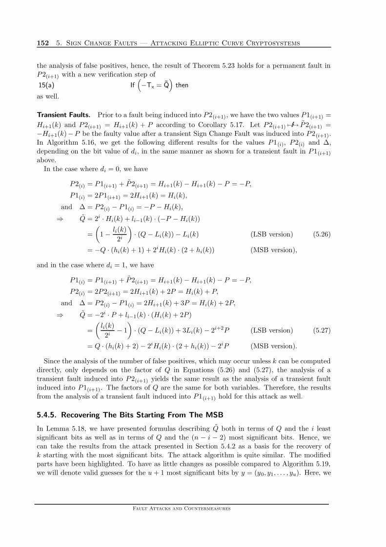
152 5. Sign Change Faults — Attacking Elliptic Curve Cryptosystems
the analysis of false positives, hence, the result of Theorem 5.23 holds for a permanent fault inP2(i+1) with a new verification step of
15(a) If(−Tx = Q
)then
as well.
Transient Faults. Prior to a fault being induced into P2(i+1), we have the two values P1(i+1) =
Hi+1(k) and P2(i+1) = Hi+1(k) + P according to Corollary 5.17. Let P2(i+1) 7−→E P2(i+1) =−Hi+1(k)−P be the faulty value after a transient Sign Change Fault was induced into P2(i+1).In Algorithm 5.16, we get the following different results for the values P1(i), P2(i) and ∆,depending on the bit value of di, in the same manner as shown for a transient fault in P1(i+1)
above.In the case where di = 0, we have
P2(i) = P1(i+1) + P2(i+1) = Hi+1(k) − Hi+1(k) − P = −P,
P1(i) = 2P1(i+1) = 2Hi+1(k) = Hi(k),
and ∆ = P2(i) − P1(i) = −P − Hi(k),
⇒ Q = 2i · Hi(k) + li−1(k) · (−P − Hi(k))
=
(1 − li(k)
2i
)· (Q − Li(k)) − Li(k) (LSB version) (5.26)
= −Q · (hi(k) + 1) + 2iHi(k) · (2 + hi(k)) (MSB version),
and in the case where di = 1, we have
P1(i) = P1(i+1) + P2(i+1) = Hi+1(k) − Hi+1(k) − P = −P,
P2(i) = 2P2(i+1) = 2Hi+1(k) + 2P = Hi(k) + P,
and ∆ = P2(i) − P1(i) = 2Hi+1(k) + 3P = Hi(k) + 2P,
⇒ Q = −2i · P + li−1(k) · (Hi(k) + 2P )
=
(li(k)
2i− 1
)· (Q − Li(k)) + 3Li(k) − 2i+2P (LSB version) (5.27)
= Q · (hi(k) + 2) − 2iHi(k) · (2 + hi(k)) − 2iP (MSB version).
Since the analysis of the number of false positives, which may occur unless k can be computeddirectly, only depends on the factor of Q in Equations (5.26) and (5.27), the analysis of atransient fault induced into P2(i+1) yields the same result as the analysis of a transient faultinduced into P1(i+1). The factors of Q are the same for both variables. Therefore, the resultsfrom the analysis of a transient fault induced into P1(i+1) hold for this attack as well.
5.4.5. Recovering The Bits Starting From The MSB
In Lemma 5.18, we have presented formulas describing Q both in terms of Q and the i leastsignificant bits as well as in terms of Q and the (n − i − 2) most significant bits. Hence, wecan take the results from the attack presented in Section 5.4.2 as a basis for the recovery ofk starting with the most significant bits. The attack algorithm is quite similar. The modifiedparts have been highlighted. To have as little changes as possible compared to Algorithm 5.19,we will denote valid guesses for the u + 1 most significant bits by y = (y0, y1, . . . , yu). Here, we
Fault Attacks and Countermeasures
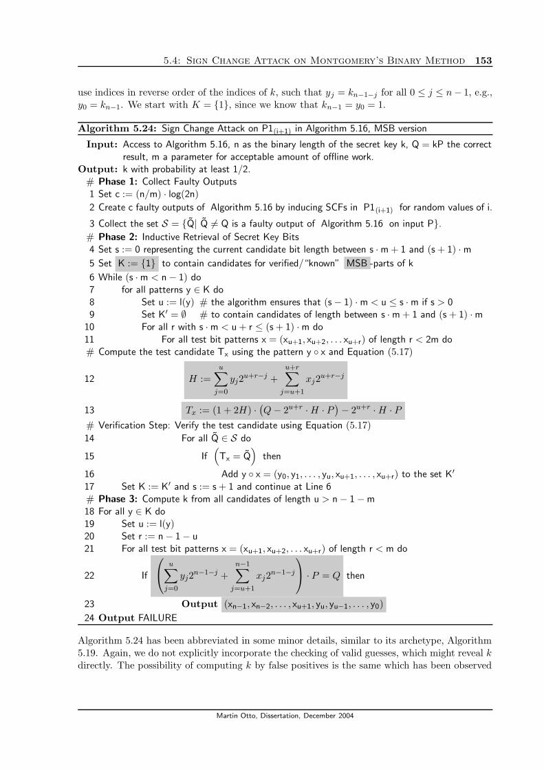
5.4: Sign Change Attack on Montgomery’s Binary Method 153
use indices in reverse order of the indices of k, such that yj = kn−1−j for all 0 ≤ j ≤ n− 1, e.g.,y0 = kn−1. We start with K = {1}, since we know that kn−1 = y0 = 1.
Algorithm 5.24: Sign Change Attack on P1(i+1) in Algorithm 5.16, MSB version
Input: Access to Algorithm 5.16, n as the binary length of the secret key k, Q = kP the correctresult, m a parameter for acceptable amount of offline work.
Output: k with probability at least 1/2.# Phase 1: Collect Faulty Outputs1 Set c := (n/m) · log(2n)
2 Create c faulty outputs of Algorithm 5.16 by inducing SCFs in P1(i+1) for random values of i.
3 Collect the set S = {Q| Q 6= Q is a faulty output of Algorithm 5.16 on input P}.# Phase 2: Inductive Retrieval of Secret Key Bits4 Set s := 0 representing the current candidate bit length between s · m + 1 and (s + 1) · m5 Set K := {1} to contain candidates for verified/“known” MSB -parts of k
6 While (s · m < n − 1) do7 for all patterns y ∈ K do8 Set u := l(y) # the algorithm ensures that (s − 1) · m < u ≤ s · m if s > 09 Set K′ = ∅ # to contain candidates of length between s · m + 1 and (s + 1) · m
10 For all r with s · m < u + r ≤ (s + 1) · m do
11 For all test bit patterns x = (xu+1, xu+2, . . . xu+r) of length r < 2m do# Compute the test candidate Tx using the pattern y ◦ x and Equation (5.17)
12 H :=
u∑
j=0
yj2u+r−j +
u+r∑
j=u+1
xj2u+r−j
13 Tx := (1 + 2H) ·(Q − 2u+r · H · P
)− 2u+r · H · P
# Verification Step: Verify the test candidate using Equation (5.17)
14 For all Q ∈ S do
15 If(Tx = Q
)then
16 Add y ◦ x = (y0, y1, . . . , yu, xu+1, . . . , xu+r) to the set K′
17 Set K := K′ and s := s + 1 and continue at Line 6# Phase 3: Compute k from all candidates of length u > n − 1 − m18 For all y ∈ K do19 Set u := l(y)20 Set r := n − 1 − u21 For all test bit patterns x = (xu+1, xu+2, . . . xu+r) of length r < m do
22 If
u∑
j=0
yj2n−1−j +
n−1∑
j=u+1
xj2n−1−j
· P = Q then
23 Output (xn−1, xn−2, . . . , xu+1, yu, yu−1, . . . , y0)
24 Output FAILURE
Algorithm 5.24 has been abbreviated in some minor details, similar to its archetype, Algorithm5.19. Again, we do not explicitly incorporate the checking of valid guesses, which might reveal kdirectly. The possibility of computing k by false positives is the same which has been observed
Martin Otto, Dissertation, December 2004

154 5. Sign Change Faults — Attacking Elliptic Curve Cryptosystems
for valid guesses in the last section and it will be described in detail below. We also do notdescribe that we only guess patterns y ◦x with a maximal length of n− 1 in Phase 2, i.e., in theloop of Lines 6–17. This has been left out to improve readability. However, it is useful in theproof of Lemma 5.25 below and adds only additional costs to search for the least significant bitk0 by exhaustive search.
To get a result similar to Theorem 5.23, we need to be able to bound the number of falsepositives which do not allow to recover k directly. This can be done with the same considerationsas for the LSB recovery, and it will be shown with the following Lemma, the twin of Lemma5.21.
Lemma 5.25 (Properties of Valid Guesses).Let x = (xn−1, xn−2, . . . , xt) and y = (yn−1, yn−2, . . . , yu) be two valid guesses for the n − t andn − u most significant bits of k. Let 1 ≤ u ≤ t ≤ n − 1 and let Q ∈ S be a faulty final resultcollected in Line 2 of Algorithm 5.24. Let
Ver(Q, x) :=
{true if Q = (1 + 2ht(x)) ·
(Q − 2tht(x)P
)− 2tht(x)P
false otherwise,
with ht(x) =∑n−1
j=t xj2j−t as defined in Definition 5.4. If Ver(Q, x) = true = Ver(Q, y), then
we have one of the following cases:
1. The two patterns x and y are equal, i.e., x = y and t = u, or
2. we have u < t andht(x) − hu(y) ≡ 0 mod #E,
i.e., the pattern y is the same as the pattern x shifted t − u bits to the right, and reducedmodulo #E, or
3. we have u ≤ t and hu(y) 6≡ ht(x) mod #E and k can be computed directly as
k ≡ (1 + ht(x)) · 2tht(x) − (1 + hu(y)) · 2uhu(y)
(ht(x) − hu(y))mod #E.
Proof:
The Lemma follows with the same arguments as in Lemma 5.21. If Ver(Q, x) = true =Ver(Q, y), we have
(1 + 2ht(x)) · (Q − 2tht(x)P ) − 2tht(x)P = (1 + 2hu(y)) · (Q − 2uhu(y)P ) − 2uhu(y)P
⇒ (1 + 2ht(x) − 1 − 2hu(y)) · k ≡ (1 + 2ht(x)) · 2tht(x) + 2tht(x)
− (1 + 2hu(y)) · 2uhu(y) − 2uhu(y)
⇒ 2 (ht(x) − hu(y)) · k ≡ (2 + 2ht(x)) · 2tht(x) (5.29)
− (2 + 2hu(y)) · 2uhu(y)
⇒ (ht(x) − hu(y)) · k ≡ (1 + ht(x)) · 2tht(x) − (1 + hu(y)) · 2uhu(y).
If ht(x) 6≡ hu(y) mod #E, the multiplicative inverse of (ht(x) − hu(y)) exists modulo #Eand k can be computed directly. If t = u and x 6= y, we always have ht(x) 6≡ hu(y).
Fault Attacks and Countermeasures

5.5: Concluding Remarks 155
For the other cases, assume w.l.o.g. that u < t. In this case, we have ht(x) ≡ hu(y) if thebits (xn−1, xn−2, . . . , xt) and the bits (yn−1−t+u, yn−2−t+u, . . . , yu) are equal and all otherbits (yn−1, yn−2, . . . , yn−t+u) are zero. Hence, y must be a shift of x to the right and reducedmodulo #E. Similar to the proof of Lemma 5.21, we may assume that both ht(x) andhu(y) are smaller than k, i.e., 0 < t, u, to ensure that ht(x) ≡ hu(y) iff ht(x) = hu(y). Thisrequires to recover the least significant bit k0 by exhaustive search, which is a negligibleamount of additional work. �
The result of Lemma 5.25 shows that the maximal number of false positives, which may occurunless k can be recovered directly, can be bounded by the same bound as stated in Lemma 5.22.Hence, Theorem 5.23 holds for the MSB attack as well.
However, the MSB attack even yields better results. Since we know that kn−1 = 1 = xn−1 =yn−1 for the two patterns x and y defined in Lemma 5.25, we know that y cannot be a shift ofx to the right, since this requires yn−1 to be equal to zero. Hence, in this case, there are nofalse positives which do not allow to recover the bits of k directly via Case 3 of Lemma 5.25.Therefore, we get the following improved version of the main result.
Theorem 5.26 (Success of the Proposed Sign Change Attack).Algorithm 5.19 succeeds to recover the secret scalar multiple k of bit length n in time O(22m ·c·M)with probability at least 1/2. Here, c = (n/m) · log(2n) and M is the maximal cost of a full scalarmultiplication or a scalar multiplication including the induction of a Sign Change Fault.
Proof:
The proof is completely analogous to the proof of Theorem 5.23 with the only modificationthat for any specific Q, there can only be at most 2 valid guesses, since any two valid guessesallow to recover k directly using Case 3 of Lemma 5.25. Case 2 of Lemma 5.25 cannotoccur. �
5.5. Concluding Remarks
All standard variants of repeated doubling have been shown to be vulnerable to Sign ChangeAttacks. The scheme of the attack follows the basic scheme from [BDL01], as presented inChapter 2. However, we have always assumed in this chapter that all faulty results Q have beencreated by attacks on algorithms with the same fixed input point P . This can be further relaxedin the same manner as in the attack described in Chapter 2. If the input point P is known tothe adversary, it is possible to use a new input point for every faulty result Q. In this case, weneed to collect pairs (Pi, Qi) in the first phase of all attack algorithms. Given such a pair, thetest value Tx must be computed with the individual input point Pi to be compared to Qi. Thiswill prevent some possible speed-ups in the attacks, but it does not have any influence on theresults.
Since we have shown that Sign Change Faults are a realistic fault model (in Section 4.5), theattacks described here are a real new threat for elliptic curve cryptosystems. These results havebeen published as a joint work with Johannes Blomer and Jean-Pierre Seifert in [BOS04].
Any new attack triggers research into appropriate countermeasures. The next chapter isdevoted to the presentation of a new countermeasure for elliptic curve cryptosystem, whichprotects specifically against Sign Change Faults.
Martin Otto, Dissertation, December 2004

156 5. Sign Change Faults — Attacking Elliptic Curve Cryptosystems
Fault Attacks and Countermeasures

6. Securing Elliptic Curve Cryptosystems
The newly developed Sign Change Fault Model has been shown to be successful in recoveringthe secret scalar factor of an elliptic curve scalar multiplication. Therefore, countermeasures areneeded. In this chapter, we will first briefly review the effectiveness of existing countermeasuresdeveloped against other side-channel attacks on elliptic curve cryptosystems in Section 6.1.Then, we will introduce a new countermeasure in Section 6.2, which has been designed toprotect elliptic curve scalar multiplication against Sign Change Faults. We will analyze theeffectiveness of this new countermeasure in Section 6.2.2.
6.1. Previously Proposed Countermeasures
We have given an overview over existing fault attacks on elliptic curve scalar multiplicationin Section 4.2. Those attacks change coordinates or curve parameters randomly. As a result,almost certainly the computed value is not a valid point on the original elliptic curve. Hence,the standard countermeasure proposed by [BMM00] and [CJ03] validates a final result beforeit is returned by a device, i.e., it simply checks whether a computed value is a valid point onthe original elliptic curve. Clearly, this countermeasure is defeated by Sign Change Faults, sincethese faults generate points which are bound to be on the original curve. Therefore, the standardcountermeasure cannot be used to protect against Sign Change Faults. Moreover, if a deviceimplements the standard countermeasure, this even helps the attacker by eliminating almost allfaulty outputs, which result from an induced fault different from a sign change. This allows theSign Change Fault Model 5.1 to be less precise in the control on location and in the number ofaffected bits.
A quite natural countermeasure against Sign Change Faults, which change the sign of they-coordinate of an intermediate point, is to use Montgomery’s binary method, where the y-coordinate is not needed (cf. [Mon87], [FGKS02]). However, several patents prevent its wide-spread application and endorse the use of other variants of repeated doubling.
Moreover, some variants of the ElGamal cryptosystem embed messages in both coordinates(cf. [GG99, § 20.6]) and may wish to use a scalar multiplication method, where both coordinatesare computed simultaneously. Additionally, there are verification schemes, which need the y-coordinate according to [IT02].
As a consequence, variants of the well-known repeated doubling algorithm, mostly based onthe non-adjacent form of the secret scalar factor, are widely employed in modern elliptic curvebased systems.
One can also use randomization schemes to counteract a fault attack with Sign Change Faults.However, smartcard certification authorities often require that algorithms are secure against faultattacks even without randomization. Moreover, randomization schemes that only randomizethe base point are not guaranteed to thwart our attacks, e.g., Coron’s third countermeasurein [Cor99, §5.3] or the proposed elliptic curve isomorphism in [JT01b, §4.1] do not defeat SignChange Attacks.
157

158 6. Securing Elliptic Curve Cryptosystems
As an alternative countermeasure against Sign Change Attacks, we propose a modified scalarmultiplication algorithm in the next section.
6.2. A New Countermeasure Against Sign Change Attacks
As a new countermeasure against Sign Change Attacks, we propose a modified repeated doublingalgorithm, which we present as Algorithm 6.1. It adds little overhead at the benefit of checkingthe correctness of the final result. Moreover, it can be based on any scalar multiplicationalgorithm which does not need field divisions. Obviously, the latter prevents the use of affinecoordinates. Hence, we will present our countermeasure in the context of projective coordinatesin the remainder of this section. We will analyze it using the NAF-based version presented asAlgorithm 5.2. The countermeasure has been motivated by Shamir’s countermeasure againstattacks on CRT-RSA exponentiations [Sha99], cf. Section 3.2.
We first explain the basic idea of our proposed countermeasure. For the modified algorithm,we assume that the curve E = Ep is defined over a prime field Fp, i.e., we have Ep := E(Fp).Furthermore, we choose a small prime t of about 60 – 80 bits to form a “small” curve Et := E(Ft).We now want to compute the scalar multiple kP in a way such that the result can easily bechecked on Et but also yields the correct result on Ep. To do so, we define an elliptic curve Ept
over the ring Zpt. This curve Ept is defined with parameters Apt and Bpt such that
Apt ≡ Ap mod p, Apt ≡ At mod t
and Bpt ≡ Bp mod p, Bpt ≡ Bt mod t.
Here, Ap and At denote the A-parameters and Bp and Bt denote the B-parameters in theWeierstrass Equation (4.5) of Ep and Et respectively. Both Apt and Bpt can be easily computedusing the Chinese Remainder Theorem, although Bpt is not needed in the addition formula. Asthe base point Pp := P is not guaranteed to exist on Et, we also choose a base point Pt on Et
and use the combined point Ppt as the base point for the scalar multiplication in Ept. Here, Ppt
is computed using the Chinese Remainder Theorem in the same manner as Apt and Bpt, i.e.,
Ppt[u] ≡ Pp[u] mod pand Ppt[u] ≡ Pt[u] mod t
for all u ∈ {x, y, z}.
We will refer to Ept as the “combined curve” of Ep and Et. Computing Q = kPpt on Ept allowsto verify the result on the small curve Et.
Algorithm 6.1: Sign Change Attack Secure Scalar Multiplication
Input: A point P on Ep, and a secret key 1 < k < ord(P)Output: kP on Ep
# offline initialization (i.e., at production time)1 Choose a prime t and an elliptic curve Et
2 Determine the combined curve Ept
# main part3 Set Q := kPpt on Ept (e.g., using Algorithm 5.2)4 Set R := kPt on Et (e.g., using Algorithm 5.2)5 If R 6= Q mod t then output FAILURE.6 else output Q on Ep
Fault Attacks and Countermeasures

6.2: A New Countermeasure Against Sign Change Attacks 159
Scalar Multiplication is used twice, once in Line 3 and once in Line 4. For the algorithm used,we assume that it features a check of the final result that returns O if the result is not a validpoint on the curve (e.g., Line 5 of Algorithm 5.2). In the case where Ept is used, we assume forsimplicity that this check is performed both modulo p and modulo t, i.e., both on Ep and on Et.
6.2.1. On the Choice of Ep and Et.
For the security of our countermeasure against Sign Change Attacks, we assume that both Ep andEt have prime order. Both curves are chosen independently, which allows to use recommendedcurves for Ep, see Table 4.1 for details on recommendations. We assume that Ep and P arechosen first. Afterwards, we choose the small curve Et with prime order. Finding such a curveEt is feasible as we will show in the following. More about finding curves with a desired ordercan be found in [BSS99, §VI.5] or [Kob91].
On Choosing Et with Prime Order.
We suggest to determine Et by choosing a triplet (At, xt, yt) ∈ Z3t uniformly at random until
the curve Et defined by that triplet has prime order. The order of such a curve Et can bedetermined in polynomial time using Schoof’s Algorithm [Sch95]. This curve Et with Bt :=y2
t − x3t − Atxt mod t and the point Pt = (xt : yt : 1) is used to compute the combined curve
Ept and to check the result in Line 5 of Algorithm 6.1. The security analysis will show that thesecurity depends on the order of Pt on Et. This does not require Et to be secret. Moreover, italso does not require #Et to be prime. It is sufficient to choose a curve Et and a point Pt suchthat the order of Pt on Et is large. We will specify a minimal size for the order of Pt on Et inSection 6.2.2.
Based on the following widely accepted conjecture, choosing #Et as a prime is practical. Ourconjecture is implied by the well-known Cramer’s conjecture, stating that π(x+log2(x))−π(x) >0 for x sufficiently large [GK86]. Here, π(x) is the prime counting function. Our conjecture hasbeen introduced in a similar setting by Goldwasser and Kilian [GK86].
Conjecture 6.2 (Number of Primes in the Hasse Interval).There exist constants c1, c2 > 0 such that
π(t + 2√
t) − π(t − 2√
t) ≥ c2
√t
logc1(t).
One could avoid using Cramer’s Conjecture by using a rather deep theorem of Heath-Brownfrom [HB78] in conjunction with choosing the prime t at random. However, this theorem usesvery large constants, which allows to use it only for very large curve orders, clearly larger thanthe curve orders currently used. The following theorem states that we can find a small curve Et
with prime order efficiently if Conjecture 6.2 holds.
Theorem 6.3 (Choosing Et with Prime Order).Let (At, xt, yt) ∈ Z3
t be chosen uniformly at random. (At, xt, yt) defines the curve Et as
Et : y2t zt ≡ x2
t + Atxtz2t + Btz
3t mod t,
where Bt := y2t − x3
t − Atxt mod t. If Conjecture 6.2 is true, then there exists a constant c > 0such that the probability that Et defined by (At, xt, yt) ∈ Z3
t has prime order is at least
c · c2
log1+c1(t),
where c1, c2 are as in Conjecture 6.2.
Martin Otto, Dissertation, December 2004

160 6. Securing Elliptic Curve Cryptosystems
Proof:
Given a triplet (At, xt, yt) ∈ F3t , we want to determine the probability that the curve Et
defined by this triplet has prime order. As the parameter At is given and xt and yt definea point P = (xt : yt : 1) on the curve, Et is uniquely defined. As zt = 1, the missing curveparameter Bt can easily be computed as Bt = y2
t − x3t − Atxt mod t.
Et is a valid elliptic curve only if the discriminant is non-zero, i.e., if gcd(4A3t +27B2
t , t) = 1.The possibility that a random triplet yields a zero discriminant is negligible: There aret2 − t different curves over Ft, each of which contains at least t − 2
√t many points. As
the curve is uniquely defined if At and any of its points Pt are fixed, there are at least(t2 − t) · (t − 2
√t) many valid triplets. As there are t3 triplets in F3
t altogether, we have
Pr[(At, xt, yt) yields a valid curve Et] ≥(t2 − t) · (t − 2
√t)
t3
= 1 −(
2√t
+1
t− 1
t√
t
)≥ 1 − 3√
t.
As this probability is negligibly far from 1, we will assume that all t3 triplets define validcurves for simplicity. By Hasse’s Theorem, we know that all possible group orders lie in theinterval [t+1−2
√t, t+1+2
√t], cf. [Sil00]. The theorem of Deuring (cf. [Len87] or [Deu41])
states that there exists a constant c′ > 0 such that there are at least c′ · (t√
t)/ log(t) manyelliptic curves for every given group order. This shows that the group orders are almostevenly distributed over all possible curves up to a factor of 1/ log(t). Among the 4
√t + 1
possible group orders, there are ∆π := π(t+1+2√
t)−π(t+1−2√
t) prime group orders,where π(x) is the prime counting function. Following Conjecture 6.2, we have c1, c2 > 0
such that ∆π ≥ c2√
tlogc1 (t) . Each of these curves is uniquely defined by its A parameter and
any of its points, i.e., there are at least t − 2√
t many triplets that define any of thesecurves. This holds because each of these curves has at least t + 1 − 2
√t many points
and O cannot be chosen in (At, xt, yt). Therefore, the probability that a random triplet(At, xt, yt) ∈ F3
t yields an elliptic curve with prime order is
Pr[#Et is prime] ≥ ∆π · c′ · t√
t · (t − 2√
t)
log(t) · t3 ≥ c′
log(t)·√
t − 2
t· c2
√t
logc1(t)
=c′ · c2
log1+c1(t)·(
1 − 2√t
)=
c · c2
log1+c1(t),
where for t > 16 we can choose c = c′/2. �
6.2.2. Analysis of the Countermeasure.
We first show that Algorithm 6.1 computes the correct result if no error occurs. Algorithm6.1 uses Et to check the result of the scalar multiplication from Line 3. If Q = kP on Ept,then Q = kP on Et as well. This is evident from modular arithmetic. Any out of the threeexceptional cases in the addition formula (P1, P2 = O or P1 = −P2) can only occur if at leastone of the intermediate results or the final result is equal to O. However, Qi = O on Ept impliesthat Qi = O on both Ep and Et. As k < #Ep, this may never happen. Hence, if no erroroccurred, Q is a valid point on both Ep and Et. Given this fact, it is straightforward to see thatR = Q on Et.
Fault Attacks and Countermeasures
6.2: A New Countermeasure Against Sign Change Attacks 161
It remains to show that the proposed algorithm is secure against known Fault Attacks. For ouranalysis, we assume that Algorithm 5.2 has been chosen as the scalar multiplication algorithm,although the result holds for other scalar multiplication algorithms as well. To counteract faultattacks with random faults induced into any of the parameters used in Line 3 of Algorithm 6.1, weimplement the countermeasure proposed by [BMM00] and [CJ03]. It requires checking whetherthe result of a scalar multiplication is a valid point on the original curve before returning a value.This check has been included as an integral part of Algorithm 5.2. Therefore, we concentrateon security against Sign Change Attacks on Line 3 of Algorithm 6.1 only. Our analysis provessecurity against Sign Change Faults only, it does not provide a general security proof or securityreduction. As it has been discussed in the introduction, a mathematical framework which allowsgeneral security claims has yet to be established.
We use the Sign Change Fault Model as defined in Definition 5.1, i.e., a Sign Change Faultcan be induced in any intermediate variable used by the scalar multiplication Q = kP on Ept.Sign Change Faults can only be induced in points of elliptic curves, the scalar k cannot beattacked. Furthermore, we assume that only a single Sign Change Fault can be induced duringeach computation of kP . We do not consider multiple attacks, as only correlated attacks in thesame run of Algorithm 6.1 would yield an advantage for an adversary. However, such attacks arenot a realistic scenario as explained in Chapter 1. The adversary can target a specific variable,e.g., Q′
i, but he cannot target a specific iteration i. As we are interested to show that a faultyvalue is returned with negligible probability, we only need to investigate Sign Change Attackson the computation in Line 3 of Algorithm 6.1. Attacks in Line 4 cannot yield a faulty outputas Q is not changed by Line 4. We first investigate the basic requirement for an error to beundetected by the countermeasure in Line 5.
Lemma 6.4 (Undetectable Sign Change Faults).Let Q = kPpt be the correct result of the scalar multiplication in Line 3 of Algorithm 6.1 and letQ = Q+κi ·P 6= Q be a faulty result from an attack on Line 3. Let rt := #Et be the group orderof Et, assumed to be prime. The faulty result Q passes by the detection mechanism in Line 5,iff rt | κi.
Proof:
Let R and Q denote the variables used in Algorithm 6.1. If rt | κi, we have κiP = O onEt. Therefore, the test R = Q in Line 5 of Algorithm 6.1 yields kPt = Q + O on Et. Asthe correct result Q satisfies Q = kPt on Et, this would not trigger a FAILURE output andthe faulty value Q would be returned. As Q 6= Q on Ept is assumed, we also have Q 6= Qon Ep. This case results in a faulty output.
If rt 6 | κi, we must show that kPt 6= Q on Et. We know that for the correct value Q, itholds that R = Q on Et. If rt 6 | κi, we have κiP 6= O on Et because rt is the prime grouporder. Therefore, the order of P is rt as well. Consequently, we have R 6= Q = Q on Et
and the security alert in Line 5 is triggered. �
Lemma 6.5 (Number of Undetectable Sign Change Faults).Let rt be the group order of Et, assumed to be prime. Let m be the blocksize used in Algorithm 5.6.Then a Sign Change Attack on Algorithm 6.1 needs a blocksize m ≥ blog(rt)c to be successful.Moreover, at most (n−1)/ blog(rt)c many undetectable faulty outputs exist. Here, it is n = l(k).
Martin Otto, Dissertation, December 2004

162 6. Securing Elliptic Curve Cryptosystems
Proof:
Assume that a Sign Change Fault was induced into Q′i for some i, resulting in a faulty
output Q1. By Equation (5.6), we have
Q1 = Q − 2Hi+1(k) = Q + κiP where κi := −2n−1∑
j=i+1
kj2j−i−1.
We further assume that rt | κi, i.e., Q1 has not been detected as a faulty value accordingto Lemma 6.4. We now consider another faulty output Q2 6= Q1 collected by Algorithm5.6. Let u 6= i denote the fault position, i.e., Q2 = Q + κuP .
We claim that for all u with |u−i| ≤ blog(rt)c, u−i 6= 0, it holds that rt 6 | κu. We considerthe two cases u < i and u > i. For u < i, we have
κu = −2
n−1∑
j=u+1
kj2j−u−1 = −2
i∑
j=u+1
kj2j−u−1 − 2
n−1∑
j=i+1
kj2j−i−1
= κi − 2 · σu, where σu :=
i∑
j=u+1
kj2j−u−1, (6.3)
and for u > i, we have
κu = −2
n−1∑
j=u+1
kj2j−u−1 = κi + 2 · ρu, where ρu :=
u∑
j=i+1
kj2j−i−1.
The value Q2 is returned only if it is an undetectable faulty result, which bypassed Line 5of Algorithm 6.1. According to Lemma 6.4, this requires that rt | κu. As we assume thatrt | κi, we need to analyze the case that rt |σu and rt | ρu respectively. We first investigateσu. Here, we have two cases: Either σu = 0 or σu > 0 over the integers. If σu = 0 over theintegers, we have κu = κi and Q1 = Q2. As this contradicts our assumption that Q1 6= Q2,we may assume that σu is not equal to 0 over the integers. If the sum in Equation (6.3) isnot equal to 0 over the integers, its absolute value must be at least as large as rt in orderto be a multiple of rt.
Exactly the same consideration holds for ρu. Both |σu| and |ρu| are smaller than 2|u−i|.Therefore, we must have |u − i| > blog(rt)c in order to have a chance that the sums |σu|and |ρu| are larger than or equal to rt. Otherwise, we cannot have rt | κi and rt | κu.
Algorithm 5.6 recovers bits in blocks of at most m bits. If it has found a valid test pattern,it starts at the position immediately following that test pattern and tries to recover thenext block of length m starting at this position. If m < blog(rt)c, the arguments aboveshows that in this block there cannot be a faulty output Q in the set S of collected faultyoutputs that satisfies the verification step. Therefore, Algorithm 5.6 needs a minimalblocksize of m = blog(rt)c in order to be able to reconstruct another faulty output Q.
As the fault positions of two undetected faulty outputs Q1 and Q2 are at least blog(rt)cbits away from each other, we have a maximum of (n− 1)/ blog(rt)c many different faultyoutputs in the set collected by Algorithm 5.6. �
Fault Attacks and Countermeasures

6.2: A New Countermeasure Against Sign Change Attacks 163
Lemma 6.5 shows that the proposed algorithm secures the scalar multiplication algorithm againstthe new Sign Change Faults if the group order of #Et is large enough. A group order of#Et > 280 guarantees that the required block size of m > 80 exceeds the acceptable amount ofoffline work significantly. For many practical applications, #Et > 260 should already be enough.
The computational overhead is acceptable. Line 3 requires computations with 30 – 40 %larger moduli (for l(p) = 192 and l(t) = 60 – 80), Line 4 requires a scalar multiplication on aconsiderably smaller curve with the scalar factor k mod #Et, which is considerably smaller thank.
As the computations in Line 3 prohibit the use of inversions, projective coordinates mustbe used. We have stated our results for the basic version of projective coordinates but otherweighted projective representations such as Jacobian or Hessian representations will do just aswell.
6.2.3. Infective Computations
It has been explained in Chapter 3 that it is desirable to avoid single points of failure. Asa possible approach to achieve this feature of an algorithm, we have reviewed the concept ofinfective computations introduced by [YKLM03] in Section 3.2.1. The explicit check proposed inLine 5 uses the zero flag as a single point of failure. However, there is an obvious way to easilymodify the algorithm to use infective computations. Lines 4, 5 and 6 could be replaced by4 Set R := (1/k mod rt) · Q − Pt on Et (using Algorithm 5.2)5 Set c := R[x] + R[y]6 Set S := cQ on Ep (using Algorithm 5.2)7 Output S
Note that if no error occurred, we have R = O = (0 : 1 : 0) in projective coordinates. Hence,c = 1 and the correct result is returned. This yields the following Algorithm, which uses infectivecomputations instead of an explicit check.
Algorithm 6.6: Sign Change Attack Secure Scalar Multiplication with Infective Computations
Input: A point P on Ep, and a secret key 1 < k < ord(P)Output: kP on Ep
# offline initialization (i.e., at production time)1 Choose a prime t and an elliptic curve Et
2 Set rt := ord(Pt) on Et
3 Determine the combined curve Ept
# main part4 Set Q := kPpt on Ept (e.g., using Algorithm 5.2)5 Set R := (1/k mod rt) · Q − Pt on Et (using Algorithm 5.2)6 Set c := R[x] + R[y]7 Set S := cQ on Ep (using Algorithm 5.2)8 Output S
Although an infective version of our countermeasure is possible, we do not recommend to useit. It has been observed in Chapter 3 that the security of an infective algorithm depends on theunpredictability of the final output. It must be computationally infeasible to trace a faulty finalresult back to secret data. This is only guaranteed if either the output is randomized using arandom number generator or if a single induced fault yields a final faulty value, which cannot be
Martin Otto, Dissertation, December 2004

164 6. Securing Elliptic Curve Cryptosystems
efficiently predicted by the adversary. If the errors, which may result from the induced faults,are from a small, efficiently sampleable set, an adversary might be able to break the system bytrying all possible error patterns and comparing the result to the final output S. This yieldsthe value c used to alter the output in Line 7 of Algorithm 6.6 to an unpredictable value. Oncec is known, it is easy to recover the faulty result Q on Ep by computing Q = 1/c · S mod #Ep.Such an attack uses the same basic principles as the attack by Boneh, DeMillo, and Liptonused in Chapters 2 and 5. A similar approach has been presented by Wagner in [Wag04], whodemonstrated that our countermeasure against Bellcore attacks against CRT-RSA is insecurefor fault models, where faults only affect a small bounded number of bits (cf. Section 3.6). Thenumber of Sign Change Faults inducable into intermediate variables used in the computationof Q on Ept in Line 4 of Algorithm 6.6 clearly is efficiently sampleable — this fact has beenused in order to develop the Sign Change Fault Attacks in Chapter 5. However, Algorithm 6.6can be used, if hardware countermeasures guarantee that only fault attacks according to theRandom Fault Model 1.9 can be mounted. The latter is currently assumed for modern high-endsmartcards (as explained in detail in Section 1.4). Once again, one can see that a smartcard isbest equipped with both, hardware and software countermeasures.
Fault Attacks and Countermeasures

7. Sign Change Attacks — RSA Revisited
In Chapter 5, we have shown that Sign Change Faults can be used successfully against ellipticcurve cryptosystems. In this chapter, we will show that in principle, the same concept can beused against the modular exponentiation algorithm in RSA, as well. Sign Change Faults aremuch harder to realize for finite field elements, but once accomplished, they allow successfulattacks on RSA signatures, which bypass a variety of commonly used countermeasures. Wehave discussed a variety of approaches to induce Sign Change Faults into elliptic curve pointsin Section 4.5. At least one of these approaches, i.e., an attack on the crypto co-processor,can change finite field values if the non-adjacent form is used for finite field multiplications.This approach can be used to change the sign of finite field elements, even for other systemsthan elliptic curve based systems. Therefore, investigating whether Sign Change Faults can beapplied to break RSA modular exponentiation is not a purely theoretic question.
In this chapter, we will show that Sign Change Faults can also be used to recover a secret RSAkey given a fault model which is stronger than the fault models used for attacks on elliptic curverepeated doubling. Additionally, we will show that this attack does not apply to both versionsof repeated squaring alike. The latter result is an example for a situation, where “downwards isbetter than upwards”, which shows that there is no generally better version of repeated squaring.This result is a negation of a result in [FV03], where a certain differential power attack promptedthe authors to state that “upwards is better than downwards”.
Algorithm 7.1: Left-to-right Rep. Squaring
Input: a message m ∈ ZN, a secret RSAkey 0 ≤ d, where l(d) denotes thebinary length of d, i.e., the numberof bits of d, and an RSA modulusN
Output: md mod N# init1 Set yl(d) := 1
# main2 For k from l(d) − 1 downto 0 do3 Set y′k := y2
k+1 mod N
4 If dk = 1 then set yk := y′k · m mod Nelse set yk := y′k mod N
5 Output y0
Algorithm 7.2: Right-to-left Rep. Squaring
Input: a message m ∈ ZN, a secret RSAkey 0 ≤ d, where l(d) denotes thebinary length of d, i.e., the numberof bits of d, and an RSA modulusN
Output: md mod N# init1 Set y−1 := 12 Set z−1 := m
# main
3 For k from 0 to l(d) − 1 do4 If dk = 1 then set yk := yk−1 · zk−1 mod N
else set yk := yk−1 mod N5 Set zk := z2
k−1 mod N
6 Output yl(d)−1
Let us first recall the standard repeated squaring algorithms, which we have presented before asAlgorithms 2.2 and 2.3. The versions presented here have been rewritten using indexed variables,in order to ensure that different uses of the same variable can be clearly distinguished.
The chances of inducing a Sign Change Fault, which changes the final result, are clearly limited
165

166 7. Sign Change Attacks — RSA Revisited
by the two Algorithms 7.2 and 7.1, since intermediate results are squared. We will investigatethe chance that a Sign Change Fault yields a faulty final result for both Algorithm separately.Our overall assumption is that during one execution of any of the two algorithms, only a singlefault can be induced.
7.1. Sign Change Faults in Left-to-Right Repeated Squaring
We first investigate Algorithm 7.1. Here, the intermediate variables yk, y′k, yk+1, and m areused. Transient faults and permanent faults have a different effect only for attacks on m, allother variables are used only once.
Sign Change in yk+1. A sign change in yk+1 results in the correct value for y′k, since y2
k+1 =−y2
k+1. Therefore, a faulty result cannot be returned.
Sign Change in y′
k. A sign change in y′k yields the negated, i.e., faulty, value yk = −y′k · mdk .
If this happens during the last iteration, where k = 0, the faulty final result −md mod N isreturned. Otherwise, the sign is eliminated in the next round, where y ′
k−1 = y2k.
Sign Change in yk. The situation for a sign change in yk is completely the same as for a signchange in y′k. It only yields a faulty final result of −md if k = 0.
Sign Change in m. The value m is used in every iteration. Therefore, transient and permanenterrors have a different effect. Although any sign change in m yields a negated value yk = −yk,this sign is eliminated in the next round, where the value yk−1 = y2
k is computed. Therefore,a sign change of m has no effect on the final result unless k = 0. Hence, a transient fault onlychanges the final result to −md mod N if it happens in iteration k = 0, while a permanent faultguarantees that −m is used in iteration k = 0. Since we have d0 = 1 for an RSA secret key, thecorrect iteration, which has been hit by a fault, cannot be determined. Therefore, we may treata permanent fault as a transient fault in iteration k = 0.
Summary. Summarizing the above considerations, it is clear that any sign change in any vari-able is corrected by the squaring in Line 3 unless it happens in the last iteration. However, thisdoes not allow to derive any information, since we know that RSA exponents are odd, hence,d0 = 1. This implies that the value y′
1 = md/m mod N is known to an adversary and he alreadyknows all the values a fault induced during this last iteration could reveal. Therefore, Algorithm7.1, the left-to-right repeated squaring algorithm, is secure against sign changes.
7.2. Sign Change Faults in Right-to-Left Repeated Squaring
For the right-to-left repeated squaring algorithm, we will analyze the effect of a sign changeof any of the intermediate variables yk−1, yk, zk−1, zk in the same manner as in the previoussection. Here, however, we will see that sign changes on certain variables yield a faulty resultregardless of the iteration.
Fault Attacks and Countermeasures

7.2: Sign Change Faults in Right-to-Left Repeated Squaring 167
Sign Change in y. A sign change in yk−1 results in the faulty value yk = −yk. This value ismultiplied with the correct powers of m in the remainder of the execution, hence, the final resultis bound to be faulty, as well. In this case, we have yl(d)−1 = −md mod N . A sign change in yk
has the exact same effect as an attack on yk−1.
Sign Change in z. Although zk−1 is used twice, both in Line 4 and in Line 5, it is not necessaryto investigate both transient and permanent faults. A sign change fault induced into zk−1 inLine 4 changes the value yk to −yk. This only holds if zk−1 is used in Line 4, i.e., when dk = 1.Since zk = z2
k−1, the value zk is always the correct value, regardless of sign changes in any ofthe two versions of zk−1 and regardless of a permanent or transient effect. Only if the variableis affected prior to its use in Line 4, the flipped sign in yk is not corrected and the final resultis the faulty value yl(d)−1 = −md mod N . A sign change in zk has exactly the same effect as afault induced into zk−1. Faults occurring during Line 5 cannot have any effect on the final resultif they occur in the last iteration.
Summary. We see that sign change faults induced into the intermediate variables used inAlgorithm 7.2 yield the negated final result for any affected iteration. However, we have also seenthat the final faulty result is independent from the affected iteration, it is always −md mod N ifthe physical attack was successful. Therefore, the only information that an adversary can get bytargeting an intermediate variable is whether an error occurred or not. We usually refer to suchfault attacks as oracle attacks, since the adversary only gets a yes/no answer for his question,whether his attack was successful or not (see Section 1.6.2). He does not get a faulty result,which allows to compute any secrets directly. The value −md mod N cannot be used to deriveany information about the secret exponent d. This is clear since any adversary is assumed toknow the correct signature md mod N , hence, he can compute −md mod N himself. This doesnot require fault attacks.
In order to retrieve information about the secret key using the oracle answer, an adversaryneeds to be able to mount an attack, where the effect of an induced fault depends heavily onthe individual secret key bits. This condition is not met for attacks on yk−1 and yk. They areused in every line, regardless of the secret key bit. For a fault induced into zk−1 however, thisis different. If the variable zk−1 is affected by a fault, the final result yl(d)−1 is correct if dk = 0and faulty if dk = 1. Therefore, if the adversary knows the iteration in which zk−1 or zk is hit,the oracle answer reveals the value of the secret key bit dk. This resembles a c-safe error asintroduced in Section 1.6.2.
In the following, we present the fault model needed for such an attack.
Definition 7.3 (Fault Model: RSA Sign Change Fault Model).We define the RSA Sign Change Fault Model with the following parameters.
location: complete control (can target the sign of a specific variable)timing: precise control (can target a specific iteration in Algorithm 7.2)number of bits: random number of faulty bits (the sign is flipped modulo N , i.e., all bits of
the affected variable may change)fault type: Sign Change Faults (see Definition 4.6)probability: certain (every physical attack results in a fault of the desired kind)duration: transient and permanent faults (both variants are possible, however, it is
assumed that an adversary cannot use both kinds during one fault attack)
Martin Otto, Dissertation, December 2004

168 7. Sign Change Attacks — RSA Revisited
The success probability of a Sign Change Fault induction may be lowered from certain to anynon-negligible probability. In such a case, the adversary has to perform many attacks on thesame iteration, until he can expect to have induced at least one successful Sign Change Fault.This requires that the adversary knows at least a non-negligible lower bound for this successprobability and increases his run time significantly. Such an attack represents a Monte-Carlo-algorithm, where every detected fault yields dk = 1 with probability 1, while a zero may bedetected incorrectly, since it is possible that all attacks were unsuccessful. With the sameconsideration, control on location and on timing could be slightly relaxed.
We have seen that Sign Change Attacks are possible in principle on RSA as well. While theleft-to-right repeated squaring version (“downwards”) is secure against Sign Change Faults, theright-to-left repeated squaring version can be attacked using Fault Model 7.3. Therefore, in thissetting, “downwards is better than upwards”.
However, one should bear in mind that such attacks face two drawbacks in practice. Onthe one hand, Sign Change Faults are much harder to realize for RSA than for elliptic curvecryptosystems. On the other hand, it requires an implementation of repeated squaring, whichallows c-safe errors using Fault Model 7.3. Even if the success probability of a Sign Change Faultinduction is lowered, Definition 7.3 represents a very strong adversary, which may be assumed tobe extremely hard to realize for modern high-end smartcards used today. Moreover, the attackon plain RSA as presented in Chapter 2 can be applied assuming less powerful adversaries.
Fault Attacks and Countermeasures

8. Conclusion and Open Problems
In this thesis, we have presented new fault attacks and new countermeasures. As a basis for theseresults, we have developed a new and comprehensive characterization of known fault models inChapter 1. This serves as a basis for both, fault attacks and countermeasures.
Fault Attacks. For the RSA cryptosystem, we have investigated the famous result for attackson the right-to-left repeated squaring algorithm presented by Boneh, DeMillo, and Lipton in[BDL01]. In Chapter 2, we have shown that the original attack contains two minor flaws, whichare due to implicit assumptions, which are not guaranteed by the original attack algorithm. Wehave corrected these flaws. Moreover, we have presented an updated version of the proof of thesuccess probability for the original attack, which we consider to be more convincing than theoriginal proof. We have also extended the attack to the left-to-right repeated squaring algorithm,proving that both versions are susceptible to fault attacks in the same way. These results roundoff the analysis of fault attacks on plain RSA in the manner described in [BDL01].
For elliptic curve cryptosystems, fault attacks have been considered to be less successful thanattacks on the RSA system. Previously reported attacks, e.g., in [BMM00] and [CJ03], representweak attacks, since they can be fended off easily. However, in Chapter 4, we have shown thatcontrary to popular believe, the standard countermeasure proposed in [BMM00] and [CJ03]does not render fault attacks useless. We have shown that undetectable faults can be inducedfor special inputs. Moreover, we have shown that undetectable faults can also be realized forarbitrary inputs using a new fault type, Sign Change Faults. We have shown that this fault typecan be induced in practice. Hence, it poses a new threat for elliptic curve cryptosystems usingrepeated doubling. In Chapter 5, we have defined a new fault model, which uses the new SignChange Faults. We have applied the new fault model to prove that fault attacks are possible ona wide variety of algorithms for computing scalar multiples of elliptic curve points. All standardalgorithms are susceptible to fault attacks in the same manner as plain RSA. Hence, we havegeneralized the results from Boneh, DeMillo, and Lipton [BDL01] to elliptic curve cryptosystems.
The new Sign Change fault type has been applied to RSA in Chapter 7. It can be usedsuccessfully for attacks on the right-to-left repeated squaring algorithm, but not for attacks onthe left-to-right repeated squaring algorithm. However, the attacks require a very strong faultmodel. Nevertheless, our results show that Sign Change Faults are a threat for RSA as well.
169

170 8. Conclusion and Open Problems
Our results about fault attacks show that a larger variety of algorithms and cryptosystemscan be successfully attacked by fault attacks than previously known.
Countermeasures. The threat posed by fault attacks is real. Hence, efficient algorithmic coun-termeasures are needed. We have developed countermeasures for the two most popular and mostwidely deployed cryptosystems, RSA and elliptic curve cryptosystems.
For RSA, we have concentrated on CRT-RSA, a fast variant of repeated squaring in Chapter3. This variant is very popular on smartcards due to its advantage in speed. However, it ishighly susceptible to fault attacks. As a consequence, we have proposed a new algorithm, whichprotects the CRT-RSA scheme against known fault attacks. The new algorithm trades speed forsecurity, however, the loss in speed is low, while the gain in security is crucial. We have provedthat the new algorithm is secure against fault attacks for the most realistic adversary, and wehave proposed modifications, which provide security even in the case of more powerful yet lessrealistic adversaries. Therefore, our new algorithm is an effective countermeasure, ready for use.The question whether our approach can also be applied for countermeasures for plain RSA isleft as an open problem.
Following our new attacks on elliptic curve cryptosystems, we have also proposed a counter-measure against these attacks in Chapter 6. We have presented an algorithm, which can secureevery scalar multiplication algorithm for elliptic curves, which does not need field inversions.This restriction is practical, since projective coordinates can be used to represent elliptic curvepoints. Projective coordinates allow to compute point multiples without using field inversions.We have proved that our new algorithm is secure against all known fault attacks on scalar mul-tiplication algorithms. Therefore, this algorithm is an effective countermeasure as well, readyto be used.
Open Problems. The major problem of fault attacks is to define a model to prove security,which is stronger than the ad-hoc security model used for proofs in this thesis, and whichis practical. In principle, the computational security model used for classic security analysis(presented in the introduction) can be used to prove security against fault attacks for specialadversaries. However, up to date such proofs are only possible for highly inefficient schemes.Such schemes are not usable in practice, hence, efficient secure schemes are needed. Currently,it is an open problem how to formalize security against fault attacks and how to capture theinformation provided by this side-channel in a mathematical framework in a practical way.Hence, research in this area should be intensified. As we have explained in Chapter 1, faultattacks are used in practice, hence, once digital signature smartcards become more popular,fault attacks will be a serious threat. This indicates the urge to not only investigate systems fortheir susceptibility to fault attacks and to develop efficient countermeasures, but also to developa better theoretical understanding of fault attacks and side-channel attacks in general.
Fault Attacks and Countermeasures

A. Detailed Fault Analysis of Affine EllipticCurve Addition
A.1. Attacks Targeting λ = (y1 − y2)/(x1 − x2)
The parameter λ, the slope of the line defined by P1 and P2, is computed using Equation (4.10),which states that
λ =y1 − y2
x1 − x2. (4.10)
Equation (4.10) computes λ using 5 variables, which can be targeted in a fault attack. As anyfault induced into the result λ has the same effect as if λ would be affected the next time it isused, the analysis of a fault induced into λ will be presented later. We first investigate faultsin the two parameters y2 and x2. Both are only used once in the whole addition formula. Wepresent the analysis of faults affecting y1 and x1 afterwards.
• Fault induced into y2:Assume that y2 is targeted by an induced fault, resulting in y2 7−→E y2 + e with e ∈ Fp. Asy2 is only used once, permanent and transient faults have the same effect and need not beconsidered separately. The induced fault enforces the usage of the faulty values λ, x3, andy3 in the computation. They take the values
λ =y1 − y2 − e
x1 − x2=
y1 − y2
x1 − x2+ e = λ + e where e :=
−e
x1 − x2
x3 = λ2 − x1 − x2 = λ2 + 2λe + e2 − x1 − x2 = x3 + 2λe + e2
y3 = −y1 + λ (x1 − x3) = −y1 + λ(x1 − x3 − 2λe − e2
)+ e
(x1 − x3 − 2λe − e2
)
= y3 + e(x1 − x3 − 2λe − e2 − 2λ2 − λe
)= y3 + e (x1 − x3 − (e + λ) (2λ + e)) .
The resulting faulty point P3 = (x3, y3) is a valid faulty point only if it satisfies theWeierstrass Equation (4.2), i.e., if y2
3 − x33 − Ax3 − B ≡ 0 mod p. This can be used to
compute e. We have
y23 − x3
3 − Ax3 − B
= e ·(
e − 2y2
x1 − x2
)·(
e2 · (x2 − x1) + 2e · (y2 − y1) +
x31 − 3x2
1x2 − Ax1 + Ax2 − 2y22 + 2x3
2 + 2y1y2
x1 − x2
)+ R,
where R = y23 − x3
3 − Ax3 − B + e · 2y1(y21 − y2
2 − x31 + x3
2 + Ax2 − Ax1)
(x1 − x2)2,
= (x2 − x1) · e ·(
e − 2y2
x1 − x2
)·(e + λ +
√2x1 + x2
)·(e + λ −
√2x1 + x2
), (A.1)
171

172 A. Detailed Fault Analysis of Affine Elliptic Curve Addition
by standard arithmetic (using Maple). Here, we have R ≡ 0. This becomes evident byapplying the Weierstrass equation, using y2
i = x3i + Axi + B for all i ∈ {1, 2, 3}. It can
be applied since we know that P1, P2, and the correct result P3 are valid points on theelliptic curve. Now, Equation (A.1) shows that we have between 2 and 4 solutions for e,since we assume that x1 6≡ x2:
e ∈{
0,2y2
x1 − x2, −λ ±
√2x1 + x2
}(A.2)
⇒ e ∈{0,−2y2, (x1 − x2) ·
(λ ±
√2x1 − x2
)}. (A.3)
The first value e = 0 can be neglected as it represents an error-free computation. Thesecond value e = −2y2 represents the case where −P2 instead of P2 is used in the additionformula. The third and fourth value exist only if the square root exists. This depends onthe input points P1 and P2.
• Fault induced into x2:Let us now assume that x2 is affected by a fault, resulting in x2 7−→E x2 + e with e ∈ Fp.Again, x2 is only used once, hence, permanent and transient faults have the same effectand need not be considered separately. This results in the following faulty value λ:
λ =y1 − y2
x1 − x2 − e=
y1 − y2
x1 − x2+ e = λ + e where e :=
e(y1 − y2)
(x1 − x2)2 − e(x1 − x2)
The latter shows that we can write λ = λ + e just as in the analysis of a fault inducedinto y2. If e ≡ (x1 −x2), the device will encounter an arithmetical error (division by zero),which will be detected as a general error. Hence, e ≡ (x1−x2) cannot create a valid faultypoint, and we may assume that e 6≡ (x1 − x2) mod p. Since the value x2 is not used again,a fault induced into x2 yields the exact same values for x3 and y3, and therefore also thesame values for e as in Equation (A.2):
e ∈{
0,2y2
x1 − x2, −λ ±
√2x1 + x2
}
⇒ e ∈{
0, 2y2 ·x1 − x2
y1 + y2, (x1 − x2) ±
(y1 − y2)√2x1 + x2
}.
Again, the solution e = 0 does not yield a valid faulty point, since it yields the correctpoint. It is therefore not a desired solution for e. The values for e exist only if thedenominators exist in Fp, i.e., if they are not equal to zero, and if the square root exists.Both depends on the input points P1 and P2. Consequently, there are between 0 and 3values for e such that a valid faulty point P3 is returned.
• Fault induced into y1:The analysis for faults induced into y1 has been presented in detail in Section 4.3.1.1.However, we will repeat the analysis briefly for completeness.
For a fault induced into the variable y1 7−→E y1 + e, e ∈ Fp, we need to investigate bothtransient and permanent faults, because y1 is used again in the computation of y3, i.e.,Equation (4.9).
Fault Attacks and Countermeasures

A.1: Attacks Targeting λ = (y1 − y2)/(x1 − x2) 173
Transient Faults. Given a transient fault, we have
λ =y1 + e − y2
x1 − x2=
y1 − y2
x1 − x2+ e = λ + e where e :=
e
x1 − x2
This represents the same situation which has been analyzed for a fault induced into y2.We can write λ as λ = λ + e, and the values of x3 and y3 are unchanged compared to afault affecting y2 as well, since the effect of the fault in y1 is transient. Therefore, we knowall possible solutions for e from Equation (A.2):
e ∈{
0,2y2
x1 − x2, −λ ±
√2x1 + x2
}
⇒ e ∈{0, 2y2, (x1 − x2) ·
(−λ ±
√2x1 + x2
)}. (A.4)
These results for e show that one transient fault which produces a valid faulty pointdepends on the value of y2, even if it is induced into y1. This is caused by the fact that y1
is used later for the computation of y3 in Equation (4.9). One might expect that negatingy1 with the error e = −2y1 would yield a valid point, since the valid input point (x1,−y1)is used. However, this does not yield a valid faulty point (x3, y3). For this to happen, thevalue y1 used in Equation (4.9) would have to be faulty as well. This requires a permanentfault, which we investigate now.
Permanent Faults. Given a permanent fault in y1, the computations of λ and x3 are thesame as shown for a fault induced into y2, but the computation of y3 is different. We getthe faulty output P3 = (x3, y3) with the values
x3 = x3 + 2λe + e2
y3 = −y1 − e + λ (x1 − x3) = y3 − e + e (x1 − x3 − e (1 + λ) (2λ + e))
= −y3 + e (x1 − x3 − e (1 + λ) (2λ + e)) − e (x1 − x2) .
As shown before, we get solutions for e by applying the Weierstrass equation (4.2), andsolving the resulting equation for e. The computation is completely analogous to theanalysis for an attack targeting y2, where we described the computation in greater detail.We have
y23 − x3
3 − Ax3 − B =
(x1 − x2) · e ·(
e +2y1
x1 − x2
)·(e + λ +
√x1 + 2x2
)·(e + λ −
√x1 + 2x2
),
with standard arithmetic (using Maple). The possible solutions for e are
e ∈{0, −2y1, (x1 − x2) ·
(−λ ±
√x1 + 2x2
)}. (A.5)
These solutions are completely symmetric to the solutions for a fault induced into y2.
Martin Otto, Dissertation, December 2004

174 A. Detailed Fault Analysis of Affine Elliptic Curve Addition
• Fault induced into x1:Finally, we assume that x1 is targeted by an attack, resulting in x1 7−→E x1 + e with e ∈ Fp.
Transient Faults. We first investigate a transient fault, i.e., we assume that when x1 isused in Equation (4.8) — the computation of x3 — it has the correct value again. We getthe following value for λ:
λ =y1 − y2
x1 + e − x2=
y1 − y2
x1 − x2+ e = λ + e where e :=
−e(y1 − y2)
(x1 − x2)2 + e(x1 − x2)
Again, the value e ≡ (x1 − x2) raises an arithmetic exception, which will be detected bythe smartcard. It cannot used to create a valid faulty result and we may assume that thiscase does not occur. As both x3 and y3 are computed using only correct values besides λ,we know the solutions for e from the analysis of a fault induced into y2, Equation (A.2).We get
e ∈{
0,2y2
x1 − x2, −λ ±
√2x1 + x2
}
⇒ e ∈{
0, −2y2 ·x1 − x2
y1 + y2, −(x1 − x2) ±
(y1 − y2)√2x1 + x2
}.
This result is the same as for a fault induced into x2, with opposite signs.
Permanent Faults. Now, we investigate the result of a permanent fault induced into x1.Here, we also use the faulty value x1 = x1 + e in Equations (4.8) and (4.9). We get
λ =y1 − y2
x1 + e − x2
x3 = λ2 − x1 − e − x2 =
(y1 − y2
x1 + e − x2
)2
− x1 − x2 − e
y3 = −y1 + λ (x1 + e − x3)
= −y1 +
(y1 − y2
x1 + e − x2
)·(
x1 + e −(
y1 − y2
x1 + e − x2
)2
+ x1 + x2 + e
)
= −y1 +
(y1 − y2
x1 + e − x2
)· (2x1 + x2 + 2e) −
(y1 − y2
x1 + e − x2
)3
.
As noted before, the value e ≡ (x2 − x1) yields an arithmetic error. Therefore, we mayassume that e 6≡ (x2 − x1). To compute solutions for e such that P3 = (x3, y3) is a validfaulty point on E, we apply the Weierstrass equation (4.2), which must hold, i.e., we solvey23 − x3
3 − Ax3 − B = 0. This is an equation with a leading term of e6. Consequently, weget six roots for e in the complex plane. The first one is the trivial root, e = 0. Two otherroots are derived from the fact that changing the x-coordinate of the input point P1 mightresult in at most two different faulty points P1, which are valid point on the elliptic curveE. They represent the intersections of the horizontal line y = y1 with the elliptic curve E,which are different from P1. In this case, the resulting point P3 is certainly a valid faulty
Fault Attacks and Countermeasures

A.2: Attacks Targeting x3 = λ2 − x1 − x2 175
point on E, because both input points are. In order to compute these points, we need tocompute all solutions of the Weierstrass Equation (4.2), i.e., we need to solve the equation
y21 ≡ x3
1 + Ax1 + B ≡ x3 + Ax + B. (A.6)
It has three roots for x. The corresponding values for e are easily derived by e = x − x1
for any solution x of Equation (A.6). The first solution, x = x1 ⇒ e = 0, is known, theothers yield the values
e = −3x1
2±√−3
4x2
1 − A.
Of the other three roots, two are complex numbers, which cannot yield a possible solutionfor e in Fp unless the imaginary part is equal to 0. The last root represents a valid valuefor e if the square root and cubic root exist for the given values of x1, x2, y1, and y2. Theformulas, however, are somewhat lengthy. They have been computed using Maple andstandard arithmetic.
e =1
2· α +
2x22
α− x1,
where α :=3
√4(y1 − y2)2 − 8x3
2 + 4(y1 − y2) ·√
(y1 − y2)2 − 4x32,
and ecomplex = −α
2− x2
2
α− x1 ±
1
2i√
3 ·(
α
2− 2x2
2
α
).
A.2. Attacks Targeting x3 = λ2− x1 − x2
The parameter x3 is computed using Equation (4.8), which states that
x3 = λ2 − x1 − x2. (4.8)
The value x2 is not used again after this line, hence, transient and permanent faults have thesame effect. The other values, x3, x1, and λ, are used again, therefore, transient and permanentfaults must be investigated separately. Note that as any fault induced into x3 in this line ofcomputation yields the same result as if it was induced into x3 in Equation (4.4), it will beanalyzed later.
• Fault induced into x1:If a fault is induced into x1 in Equation (4.3), we have x1 7−→E x1 + e, e ∈ Fp, i.e.,
x3 = λ2 − (x1 + e) − x2 = x3 − e
and y3 = −y1 + λ · (x1 − (x3 − e)) = y3 + λe, in case of a transient fault,
or y3 = −y1 + λ · (x1 + e − (x3 − e)) = y3 + 2λe in case of a permanent fault.
Transient Faults. We first investigate a transient fault. In order for (x3, y3) to be a validpoint on the curve, it has to satisfy the Weierstrass Equation (4.2), i.e., it must hold that
y2 ≡ x3 + Ax + B mod p.
Martin Otto, Dissertation, December 2004

176 A. Detailed Fault Analysis of Affine Elliptic Curve Addition
⇒ e3 + e2(λ2 − 3x3
)+ e
(3x2
3 + A + 2y3λ)≡ 0 mod p
⇒ e ∈{
0,3x3 − λ2
2± 1
2
√λ4 − 6λ2x3 − 3x2
3 − 4A − 8y3λ
}mod p. (A.7)
Again, these formulas have been computed using standard arithmetic. Since e ≡ 0 doesnot yield a valid faulty point, we only have possible values for e if the square root exists.
Permanent Faults. If the fault is permanent, the result follows in the same manner.Here, e must satisfy
e ∈{
0,3x3 − 2λ2
2± 1
2
√16λ4 − 24λ2x3 − 3x2
3 − 4A − 16y3λ
}mod p. (A.8)
In both cases the result e = 0 represents the correct result, it cannot yield a valid faultyresult.
• Fault induced into x2:If x2 7−→E x2 + e, e ∈ Fp, is hit during a fault attack, we have the same situation as for afault induced into x1, with the only difference that transient faults and permanent faultsyield the same result as a transient fault on x1. This is due to the fact that x2 is no longerused after the computation of x3. Hence, we have x3 = x3−e and y3 = y3 +λe. Therefore,we get the solutions
e ∈{
0,3x3 − λ2
2± 1
2
√λ4 − 6λ2x3 − 3x2
3 − 4A − 8y3λ
}mod p.
• Fault induced into λ:The analysis of a fault being induced into λ has been presented in detail in Section 4.3.1.2.However, we will repeat the analysis briefly for completeness.
For faults affecting λ, we investigate three different cases. First, the variable λ could havebeen affected prior to its first use in Equation (4.8). The effect of the induced fault couldbe transient or permanent. But then, it could also be that the result λ2 could have beenaffected by the fault. We will investigate a fault affecting λ first. In this case, the faultyvalue λ + e is used and we get the faulty results
x3 = (λ + e) − x1 − x2 = x3 + 2λe + e2
and y3 = −y1 + λ ·(x1 − (x3 + 2λe + e2)
)
= y3 − 2λ2e − λe2 in case of a transient fault,
or y3 = −y1 + (λ + e) ·(x1 − (x3 + 2λe + e2)
)
= y3 + e(x1 − x3 − 2λe − e2 − 2λ2 − λe
)
= y3 + e (x1 − x3 − (2λ + e) · (e + λ)) in case of a permanent fault.
Transient Faults. Let e := −2λe− e2. In this case, the resulting faulty point P3 is equalto (x3 − e, y3 + λe). This situation is the same as the one analyzed for a transient fault
Fault Attacks and Countermeasures

A.3: Attacks Targeting y3 = −y1 + λ · (x1 − x3) 177
induced into x1 in the computation of x3. The analysis resulted in Equation (A.7), whichyields the condition
e ∈{
0,3x3 − λ2
2± 1
2
√λ4 − 6λ2x3 − 3x2
3 − 4A − 8y3λ
}mod p.
As e is a quadratic equation in e, this yields 6 possible solutions for e, namely
e ∈{
0,−2λ,−λ ±√
3
2(λ2 − x3) ±
√λ4 − 6λ2x3 − 3x2
3 − 4A − 8y3λ
}mod p. (A.9)
Permanent Faults. For permanent faults in λ, the situation is the same as for a faultinduced into y2 in the computation of λ = (y2 − y1)/(x2 − x1). It has been analyzed thereyielding the conditions stated in Equation (A.2):
e ∈{
0,2y2
x1 − x2, −λ ±
√y21 − y2
2 + x31 − 3x2
1x2 − Ax1 + Ax2 − 2x32
x1 − x2
}
Attack targeting λ2. As the value λ is squared in the computation of x3, it is alsopossible that the final result λ2 is affected by an induced fault. In this case, we haveλ2 7−→E λ2 + e, for some e ∈ Fp. As the value λ2 is only used once, we do not need todifferentiate between transient and permanent faults. This situation can be expressed bythe formulas
x′3 = λ2 + e − x1 − x2 = x3 + e
y′3 = −y1 + λ · (x1 − x3 − e) = y3 − λe.
Setting e = −e yields the faulty result P3 = (x3 − e, y3 + λe). It has been analyzed beforewhen a transient fault in x1 in the computation of x3 has been assumed. The analysisresulted in Equation (A.7), which states the condition
e ∈{
0,3x3 − λ2
2± 1
2
√λ4 − 6λ2x3 − 3x2
3 − 4A − 8y3λ
}mod p.
⇒ e ∈{
0,λ2 − 3x3
2± 1
2
√λ4 − 6λ2x3 − 3x2
3 − 4A − 8y3λ
}mod p.
A.3. Attacks Targeting y3 = −y1 + λ · (x1 − x3)
In Equation (4.9), y3 is computed using the four variables y1, λ, x1, and x3 as
y3 = −y1 + λ (x1 − x3) . (4.9)
The three variables y1, λ, x1 and y3 are no longer used in the addition formula after this lineof computation, therefore, we need not differentiate between transient and permanent faults.The value of x3, however, is used afterwards when the resulting point P3 = (x3, y3) is returnedby the addition formula. Therefore, in the case of x3, a differentiation between transient andpermanent faults is necessary.
Martin Otto, Dissertation, December 2004
178 A. Detailed Fault Analysis of Affine Elliptic Curve Addition
• Fault induced into y1:If a fault is induced into y1 in Equation (4.9), we have
y3 = −y1 + e + λ · (x1 − x3) = y3 + e,
for e ∈ Fp.
We know that for a fixed x3-coordinate only the intersections of the vertical line at x =x3 with the elliptic curve E yield valid points. For any line, there exist at most threeintersections with the elliptic curve, which are the correct point P3 = (x3, y3), the negatedpoint −P3 = (x3,−y3) and the point at infinity O. As O is a special point speciallytreated in affine coordinates, it cannot be represented by a tuple from F2
p. Therefore, wemay assume that it cannot be created by any fault which changes coordinates within Fp.This implies that the only possibility for e to yield a valid faulty point P3 on E is that thesign of y3 is flipped by that fault. This requires that y3 := y3 + e ≡ −y3 mod p, hence,
e ≡ −2y3 mod p. (A.10)
• Fault induced into λ:Given a fault induced into the slope λ in Equation (4.9), we have
y3 = −y1 + (λ + e) · (x1 − x3) = y3 + e · (x1 − x3) ,
where e ∈ Fp.
The only possibility for P3 = (x3, y3) to be a valid point on E is that y3 = −y3. Thisimplies that −2y3 = e · (x1 − x3). If x1 −x3 = 0, which may only happen if P1 = ±P3, theerror has no effect, and the correct result y3 is returned. We may therefore assume thatx1 6= x3 and conclude that a valid faulty point on E results only for
e ≡ −2y3/(x1 − x3) mod p if x1 6= x3.
• Fault induced into x1:A fault induced into the point coordinate x1 in Equation (4.9) yields
y3 = −y1 + λ · (x1 + e − x3) = y3 + eλ,
with e ∈ Fp.
In order for y3 to be equal to −y3, the error e must satisfy
e ≡ −2y3/λ mod p if y1 6= y2.
Note that if λ ≡ 0, the error would not have any effect and the correct value would bereturned.
• Fault induced into x3:As the variable x3 is used after the computation for Equation (4.9), we differentiate betweena transient fault in x3 and a permanent fault in x3. For a transient fault, the pointP3 = (x3, y3) is returned, for a permanent fault, the output is P3 = (x3, y3) = (x3 + e, y3).
In both cases, we have
y3 = −y1 + λ · (x1 − x3 − e) = y3 − eλ,
for e ∈ Fp.
Fault Attacks and Countermeasures

A.3: Attacks Targeting y3 = −y1 + λ · (x1 − x3) 179
Transient Faults. Given a transient fault, a valid faulty point P3 is returned only ify3 = −y3, hence, if
e ≡ 2y3/λ mod p if y1 6= y2.
Not surprisingly, this is the same result as for a fault induced into x1 with opposite signs.Again, we may assume that λ 6= 0 as otherwise the error would not have any effect andthe correct value would be returned.
Permanent Faults. Given a permanent fault, a faulty point P3 = (x3, y3) is returned,where
x3 = x3 + e
y3 = −y1 + λ · (x1 − x3 − e) = y3 − eλ.
Again, we have e ∈ Fp. With e := −e, this situation is the same as the one analyzedfor a transient fault induced into x1 in the computation of x3. Equation (A.7) states thecondition
e ∈{
0,3x3 − λ2
2± 1
2
√λ4 − 6λ2x3 − 3x2
3 − 4A − 8y3λ
}mod p.
⇒ e ∈{
0,λ2 − 3x3
2± 1
2
√λ4 − 6λ2x3 − 3x2
3 − 4A − 8y3λ
}mod p.
• Fault induced into y3:Given a fault induced into the final y-coordinate y3 in Equation (4.4), we have
y3 = y3 + e,
where e ∈ Fp.
Again, the only possibility for P3 = (x3, y3) to be a valid point on E is that y3 = y3 + e =−y3. This implies that
e ≡ −2y3 mod p. (A.11)
Martin Otto, Dissertation, December 2004

180 A. Detailed Fault Analysis of Affine Elliptic Curve Addition
Fault Attacks and Countermeasures

Bibliography
[ABF+02] Christian Aumuller, Peter Bier, Wieland Fischer, Peter Hofreiter, and Jean-Pierre Seifert, Fault attacks onRSA with CRT: Concrete results and practical countermeasures, Cryptographic Hardware and EmbeddedSystems — CHES 2002 (B. S. Kaliski, Jr., C.K. Koc, and C. Paar, eds.), Lecture Notes in ComputerScience, vol. 2523, Springer-Verlag, 2002, pp. 260–275.
[AK96] Ross J. Anderson and Markus G. Kuhn, Tamper resistance – a cautionary note, Proceedings of the SecondUSENIX Workshop on Electronic Commerce (Oakland, California), USENIX Association, November 18-211996, pp. 1 – 11.
[AK97] Ross J. Anderson and Markus G. Kuhn, Low cost attacks on tamper resistant devices, Security Proto-cols, 5th International Workshop, Paris, France, April 7-9, 1997 (M. Lomas et al., ed.), Lecture Notes inComputer Science, vol. 1361, Springer-Verlag, 1997, pp. 125–136.
[ANS99] ANSI X9.63-199x: Public key cryptography for the financial services industry: Key agreement and keytransport using elliptic curve cryptography, american bankers association, 8 January 1999, Working Draft,http://cnscenter.future.co.kr/resource/crypto/standard/ansi x9/x9-63-01-08-99.pdf.
[Bar96] Paul Barrett, Implementing the Rivest Shamir and Adleman public key encryption algorithm on a standarddigital signal processor, Advances in Cryptology — CRYPTO’86 (A. M. Odlyzko, ed.), Lecture Notes inComputer Science, vol. 263, Springer-Verlag, 1996, pp. 311–323.
[BCN+04] Hagai Bar-El, Hamid Choukri, David Naccache, Michael Tunstall, and Claire Whelan, The sorcerer’sapprentice guide to fault attacks, Cryptology ePrint Archive, Report 2004/100, 2004, http://eprint.
iacr.org/2004/100/.
[BD00] Dan Boneh and Glenn Durfee, Cryptanalysis of RSA with private key d less than N 0.292 , IEEE Transactionson Information Theory 46 (2000), no. 4, 1339–1349.
[BDH+98] Feng Bao, Robert H. Deng, Yongfei Han, Albert B. Jeng, A. Desai Narasimhalu, and Teow-Hin Ngair,Breaking public key cryptosystems on tamper resistant devices in the presence of transient faults, SecurityProtocols Workshop 1997 (B. Christianson, B. Crispo, T.M.A. Lomas, and M. Roe, eds.), Lecture Notesin Computer Science, vol. 1361, Springer-Verlag, 1998, pp. 115–124.
[BDL97] Dan Boneh, Richard A. DeMillo, and Richard J. Lipton, On the importance of checking cryptographic pro-tocols for faults, Advances in Cryptology — EUROCRYPT’97 (W. Fumy, ed.), Lecture Notes in ComputerScience, vol. 1233, Springer-Verlag, 1997, pp. 37–51.
[BDL01] Dan Boneh, Richard A. DeMillo, and Richard J. Lipton, On the importance of eliminating errors incryptographic computations, J. Cryptology 14 (2001), no. 2, 101–119. MR 1 830 690
[BM04] Johannes Blomer and Alexander May, A generalized Wiener attack on RSA, Public Key Cryptography —PKC 2004 (F. Bao, R. Deng, and J. Zhou, eds.), Lecture Notes in Computer Science, vol. 2947, Springer-Verlag, 2004, pp. 1–13.
[BMM00] Ingrid Biehl, Bernd Meyer, and Volker Muller, Differential fault attacks on elliptic curve cryptosystems,Advances in Cryptology — CRYPTO 2000 (Mihir Bellare, ed.), Lecture Notes in Computer Science, vol.1880, Springer-Verlag, 2000, pp. 131–146.
[Boo51] Andrew D. Booth, A signed binary multiplication technique, Quart. Journ. Mech. and Applied Math. IV(1951), no. 2, 236–240.
[BOPV03] Lejla Batina, Siddika B. Ors, Bart Preneel, and Joos Vandewalle, Hardware architectures for public keycryptography, Integration, the VLSI Journal 34 (2003), no. 1–2, 1–64.
[BOS03] Johannes Blomer, Martin Otto, and Jean-Pierre Seifert, A new CRT-RSA algorithm secure against Bellcoreattacks, Conference on Computer and Communications Security — CCS 2003 (V. Atluri and P. Liu, eds.),ACM SIGSAC, ACM Press, 2003, pp. 311–320.
181

182 Bibliography
[BOS04] Johannes Blomer, Martin Otto, and Jean-Pierre Seifert, Sign change fault attacks on elliptic curve cryp-tosystems, Cryptology ePrint Archive, Report 2004/227, 2004, http://eprint.iacr.org/2004/227/.
[BR95a] Mihir Bellare and Phillip Rogaway, Optimal asymmetric encryption, Advances in cryptology — EURO-CRYPT ’94, Lecture Notes in Computer Science, Springer-Verlag, 1995, pp. 92–111. MR 98i:94016
[BR95b] Mihir Bellare and Phillip Rogaway, Optimal Asymmetric Encryption — how to encrypt with RSA, http://www-cse.ucsd.edu/users/mihir/papers/oae.ps.gz, an extended abstract of this paper has been publishedas [BR95a], 1995.
[BS97] Eli Biham and Adi Shamir, Differential fault analysis of secret key cryptosystems, Advances in Cryptology— CRYPTO ’97 (B. S. Kaliski, Jr., ed.), Lecture Notes in Computer Science, vol. 1294, Springer-Verlag,1997, pp. 513–525.
[BS03] Johannes Blomer and Jean-Pierre Seifert, Fault based cryptanalysis of the Advanced Encryption Standard(AES), Financial Cryptography — FC 2003, Lecture Notes in Computer Science, vol. 2742, Springer-Verlag,2003, pp. 162–181.
[BSS99] Ian Blake, Gadiel Seroussi, and Nigel Smart, Elliptic curves in cryptography, London Mathematical SocietyLecture Note Series, vol. 265, Cambridge University Press, 1999.
[CC86] David V. Chudnovsky and Gregory V. Chudnovsky, Sequences of numbers generated by addition in formalgroups and new primality and factorization tests, Advances in Applied Mathematics 7 (1986), no. 4,385–434.
[CCD00] Christophe Clavier, Jean-Sebastien Coron, and Nora Dabbous, Differential power analysis in the presenceof hardware countermeasures, Cryptographic Hardware and Embedded Systems — CHES 2000, LectureNotes in Computer Science, vol. 1965, Springer-Verlag, 2000, pp. 252–263.
[CCJ03] Benoıt Chevallier-Mames, Mathieu Ciet, and Marc Joye, Low-cost solutions for preventing simple side-channel analysis: Side-channel atomicity, Cryptology ePrint Archive, Report 2003/237, 2003, http://
eprint.iacr.org/2003/237/.
[Cer00] Certicom, Current public-key cryptographical systems — the elliptic curve cryptosystem, A Cer-ticom Whitepaper, July 2000, http://www.inf.pucrs.br/∼eduardob/disciplinas/tc/luis aristeu/
docs/EccWhite2.pdf.
[CJ03] Mathieu Ciet and Marc Joye, Elliptic curve cryptosystems in the presence of permanent and transientfaults, Cryptology ePrint Archive, Report 2003/028, 2003, http://eprint.iacr.org/2003/028/.
[CJRR99] Suresh Chari, Charanjit S. Jutla, Josyula R. Rao, and Pankaj Rohatgi, Towards sound approaches tocounteract power-analysis attacks, Advances in Cryptology — CRYPTO ’99 (M. Wiener, ed.), LectureNotes in Computer Science, vol. 1666, Springer-Verlag, 1999, pp. 398–412.
[CKN00] Jean-Sebastien Coron, Paul C. Kocher, and David Naccache, Statistics and secret leakage, Financial Cryp-tography — FC 2000 (Y. Frankel, ed.), Lecture Notes in Computer Science, vol. 1962, Springer-Verlag,2000, p. 157 ff.
[CMO98] Henri Cohen, Atsuko Miyaji, and Takatoshi Ono, Efficient elliptic curve exponentiation using mixed coordi-nates, Advances in Cryptology — ASIACRYPT’98 (K. Ohta and D. Pei, eds.), Lecture Notes in ComputerScience, vol. 1514, Springer-Verlag, 1998, pp. 51–65.
[Cor99] Jean-Sebastien Coron, Resistance against differential power analysis for elliptic curve cryptosystems, Cryp-tographic Hardware and Embedded Systems — CHES ’99 (C.K. Koc and C. Paar, eds.), Lecture Notes inComputer Science, vol. 1717, Springer-Verlag, 1999, pp. 292–302.
[CQ82] Christophe Couvreur and Jean-Jacques Quisquater, Fast decipherment algorithm for RSA public-key cryp-tosystem, Electronic Letters 18 (1982), no. 21, 905–907.
[Deu41] Max Deuring, Die Typen der Multiplikatorenringe elliptischer Funktionenkorper, Abh. Math. Sem. Han-sischen Univ. 41 (1941), 197–272.
[DH76] Whitfield Diffie and Martin E. Hellman, New directions in cryptography, IEEE Transactions on InformationTheory IT-22 (1976), no. 6, 644–654.
[DLS81] Peter J. Downey, Benton L. Leong, and Ravi Sethi, Computing sequences with addition chains, SIAM J.Comput. 10 (1981), no. 3, 638 – 646.
Fault Attacks and Countermeasures

Bibliography 183
[Dot02] Emmanuelle Dottax, Fault attacks on NESSIE signature and identification schemes, NESSIE public re-port Nr. NES/DOC/ENS/WP5/031/1, 8 Oct 2002, https://www.cosic.esat.kuleuven.ac.be/nessie/
reports/phase2/SideChan 1.pdf.
[EK90] Omer Egecioglu and Cetin K. Koc, Fast modular exponentiation, Communication, Control, and SignalProcessing (1990), 188 – 194.
[ElG85] Taher ElGamal, A public key cryptosystem and a signature scheme based on discrete logarithms, IEEETransactions on Information Theory 31 (1985), 469–472.
[FGKS02] Wieland Fischer, Christophe Giraud, Erik W. Knudsen, and Jean-Pierre Seifert, Parallel scalar multipli-cation on general elliptic curves over Fp hedged against non-differential side-channel attacks, CryptologyePrint Archive, Report 2002/007, 2002, http://eprint.iacr.org/2002/007/.
[FIP00] U.S. Department of Commerce/National Institute of Standards and Technology (NIST): Digital SignatureStandard (DSS), Federal Information Processing Standards Publication (FIPS PUB 186.2), 2000, http:
//csrc.nist.gov/publications/fips/fips186-2/fips186-2-change1.pdf.
[FS02] Wieland Fischer and Jean-Pierre Seifert, Note on fast computation of secret RSA exponents, 7th Aus-tralasian Conference on Information Security and Privacy — ACISP 2002 (L. Batten and J. Seberry, eds.),Lecture Notes in Computer Science, vol. 2384, Springer-Verlag, 2002, pp. 136–143.
[FSM99] FSTC eCheck Initiative: full FSML 1.5 reference specification, 1999, http://www.echeck.org/library/
ref/fsml-v1500a.pdf.
[FV03] Pierre-Alain Fouque and Frederic Valette, The doubling attack — why upwards is better than downwards,Cryptographic Hardware and Embedded Systems — CHES 2003 (Colin D. Walter, Cetin K. Koc, andChristof Paar, eds.), Lecture Notes in Computer Science, vol. 2779, Springer-Verlag, 2003, pp. 269–280.
[GA03] Sudhakar Govindavajhala and Andrew W. Appel, Using memory errors to attack a virtual machine,Proceedings of the IEEE Symposium on Security and Privacy, May 2003, pp. 154–164.
[Gal99] Robert Gallant, Faster elliptic curve cryptography using efficient endomorphisms, Presentation at ECC’99,1999, http://www.cacr.math.uwaterloo.ca/conferences/1999/ecc99/gallant.ps.
[Gar59] Harvey L. Garner, The residue number system, IRE Transactions on Electronic Computers EC-8 (1959),no. 6, 140–147.
[GG99] Joachim von zur Gathen and Jurgen Gerhard, Modern computer algebra, Cambridge University Press,1999.
[GK86] Shafi Goldwasser and Joe Kilian, Almost all primes can be quickly certified, ACM Symposium on Theoryof Computing — STOC ’86, ACM Press, 1986, pp. 316–329.
[GK04] Christophe Giraud and Erik W. Knudsen, Fault attacks on signature schemes, Information Security andPrivacy: 9th Australasian Conference — ACISP 2004 (Huaxiong Wang, Josef Pieprzyk, and Vijay Varad-harajan, eds.), Lecture Notes in Computer Science, vol. 3108, Springer-Verlag, 2004, pp. 478–491.
[GMO01] Karine Gandolfi, Christophe Mourtel, and Francis Olivier, Electromagnetic analysis: Concrete results,Cryptographic Hardware and Embedded Systems — CHES 2001 (C.K. Koc, D. Naccache, and C. Paar,eds.), Lecture Notes in Computer Science, vol. 2162, Springer-Verlag, 2001, pp. 251–272.
[Gor98] Daniel M. Gordon, A survey of fast exponentiation methods, Journal of Algorithms 27 (1998), 129 – 146,Article No. AL970913.
[HB78] David R. Heath-Brown, The differences between consecutive primes, J. London Math. Soc. 18 (1978),no. 2, 7–13.
[HL22] Godfrey H. Hardy and John E. Littlewood, Some problems of ’Partitio Numerorum’ III: On the expressionof a number as a sum of primes, Acta Mathematica, vol. 44, 1922, pp. 1–70.
[HMV04] Darrel Hankerson, Alfred J. Menezes, and Scott A. Vanstone, Guide to elliptic curve cryptography, SpringerProfessional Computing, Springer-Verlag, 2004.
[HP98] Helena Handschuh and Pascal Pailler, Smart card crypto-coprocessors for public-key cryptography, Proc.of CARDIS ’98, Lecture Notes in Computer Science, vol. 1820, Springer-Verlag, 1998, pp. 372–379.
Martin Otto, Dissertation, December 2004

184 Bibliography
[HPS99] Helena Handschuh, Pascal Paillier, and Jacques Stern, Probing attacks on tamper-resistant devices, Cryp-tographic Hardware and Embedded Systems — CHES ’99 (C.K. Koc and C. Paar, eds.), Lecture Notes inComputer Science, vol. 1717, Springer-Verlag, 1999, pp. 303–315.
[Hwa79] Kai Hwang, Computer arithmetic: principles, architecture and design, John Wiley & Sons, 1979.
[IEE98] IEEE P1363/D3 (Draft Version 3), Standard specifications for public key cryptography, May 1998.
[IEE99] IEEE P1363/D13 (Draft Version 13), Standard specifications for public key cryptography, November 1999.
[IPS01] IPSec Working Group: Additional ECC groups for IKE, March 2001, Working Group draft, http://
cnscenter.future.co.kr/resource/ietf/wg-draft/draft-ietf-ipsec-ike-ecc-groups-03.txt.
[ISO02a] International Organization for Standardization, ISO/IEC 7816-2: Dimensions and location of the contacts,2002, http://www.iso.ch.
[ISO02b] International Organization for Standardization, ISO/IEC 7816-3: Electronic signals and transmissionprotocols, 2002, http://www.iso.ch.
[IT02] Tetsuya Izu and Tsuyoshi Takagi, A fast parallel elliptic curve multiplication resistant against side channelattacks, Public Key Cryptography — PKC 2002 (D. Naccache and P. Paillier, eds.), Lecture Notes inComputer Science, vol. 2274, Springer-Verlag, 2002, pp. 280–296.
[IT03] Tetsuya Izu and Tsuyoshi Takagi, Exceptional procedure attack on elliptic curve cryptosystems, PublicKey Cryptography — PKC 2003 (Y.G. Desmedt, ed.), Lecture Notes in Computer Science, vol. 2567,Springer-Verlag, 2003, pp. 224–239.
[Itk02] Gene Itkis, Intrusion-resilient signatures: Generic constructions, or defeating strong adversary with mini-mal assumptions, Security in Communication Networks — SCN 2002 (S. Cimato, C. Galdi, and G. Persiano,eds.), Lecture Notes in Computer Science, vol. 2576, Springer-Verlag, 2002, pp. 102–118.
[Itk03] Gene Itkis, Cryptographic tamper evidence, Proceedings of CCS 2003 (Vijay Atluri and Peng Liu, eds.),ACM SIGSAC, ACM press, Oct 2003, pp. 255–364.
[JBF02] Matthias Jacob, Dan Boneh, and Edward Felten, Attacking an obfuscated cipher by injecting faults, Dig-ital Rights Management — DRM 2002, ACM CCS-9 Workshop (J. Feigenbaum, ed.), Lecture Notes inComputer Science, vol. 2696, Springer-Verlag, 2002, pp. 16–31.
[JKQ97] Marc Joye, Francois Koeune, and Jean-Jacques Quisquater, Further results on Chinese remaindering, Tech.Report CG-1997/1, UCL Microelectronics Laboratory — Crypto Group, March 1997, http://www.dice.
ucl.ac.be/crypto/tech reports/CG1997 1.ps.gz.
[JLQ99] Marc Joye, Arjen K. Lenstra, and Jean-Jacques Quisquater, Chinese remaindering cryptosystems in thepresence of faults, Journal of Cryptology 12 (1999), no. 4, 241–245.
[JQ96] Marc Joye and Jean-Jacques Quisquater, Attacks on systems using Chinese remaindering, Tech. Re-port CG-1996/9, UCL Microelectronics Laboratory — Crypto Group, 1996, http://www.dice.ucl.ac.
be/crypto/tech reports/CG1996 9.ps.gz.
[JQ97a] Marc Joye and Jean-Jacques Quisquater, Faulty RSA encryption, Tech. Report CG-1997/8, UCL Mi-croelectronics Laboratory — Crypto Group, 1997, http://www.dice.ucl.ac.be/crypto/tech reports/
CG1997 8.ps.gz.
[JQ97b] Marc Joye and Jean-Jacques Quisquater, RSA-type signatures in the presence of transient faults, Tech.Report CG-1997/7, UCL Microelectronics Laboratory — Crypto Group, July 1997, http://www.dice.
ucl.ac.be./crypto/tech reports/CG1997 7.ps.gz.
[JQ01] Marc Joye and Jean-Jacques Quisquater, Hessian elliptic curves and side-channel attacks, CryptographicHardware and Embedded Systems — CHES 2001 (C.K. Koc, D. Naccache, and C. Paar, eds.), LectureNotes in Computer Science, vol. 2162, Springer-Verlag, 2001, pp. 412–420.
[JQBD97] Marc Joye, Jean-Jacques Quisquater, Feng Bao, and Robert H. Deng, RSA-type signatures in the presenceof transient faults, Cryptography and Coding (M. Darnell, ed.), Lecture Notes in Computer Science, vol.1355, Springer-Verlag, 1997, pp. 155–160.
[JQYY02] Marc Joye, Jean-Jacques Quisquater, Sung-Ming Yen, and Moti Yung, Observability analysis: Detectingwhen improved cryptosystems fail, Topics in Cryptology — CT-RSA 2002 (B. Preneel, ed.), Lecture Notesin Computer Science, vol. 2271, Springer-Verlag, February 2002, pp. 17–29.
Fault Attacks and Countermeasures

Bibliography 185
[JT01a] Marc Joye and Christophe Tymen, Compact encoding of non-adjacent forms with applications to ellipticcurve cryptography, Cryptographic Hardware and Embedded Systems — CHES 2001 (C.K. Koc, D. Nac-cache, and C. Paar, eds.), Lecture Notes in Computer Science, vol. 2162, Springer-Verlag, 2001, pp. 377–390.
[JT01b] Marc Joye and Christophe Tymen, Protections against differential analysis for elliptic curve cryptography— an algebraic approach, Advances in Cryptology — CRYPTO 2001 (C. K. Koc, D. Naccache, and C. Paar,eds.), Lecture Notes in Computer Science, vol. 2162, Springer-Verlag, 2001, pp. 377–390.
[JY00] Marc Joye and Sung-Ming Yen, Optimal left-to-right binary signed-digit recoding, IEEE Transactions onComputers 49 (2000), no. 7, 740–748.
[Kal03] Burt S. Kaliski, Jr., TWIRL and RSA key size, 2003, RSA Laboratories Technical Notes, http://www.
rsasecurity.com/rsalabs/node.asp?id=2004.
[KJJ99] Paul C. Kocher, Joshua Jaffe, and Benjamin Jun, Differential power analysis, Advances in Cryptology— CRYPTO ’99 (M. Wiener, ed.), Lecture Notes in Computer Science, vol. 1666, Springer-Verlag, 1999,pp. 388–397.
[KK99] Oliver Kommerling and Markus G. Kuhn, Design principles for tamper-resistant smartcard processors,Proceedings of the USENIX Workshop on Smartcard Technology — Smartcard ’99, USENIX Association,1999, pp. 9–20.
[KKT04] Mark Karpovsky, Konrad J. Kulikowski, and Alexander Taubin, Robust protection against fault-injectionattacks on smart cards implementing the advanced encryption standard, International Conference on De-pendable Systems and Networks — DSN’04, IEEE Computer Society, 2004, pp. 93–101.
[Kob87] Neil Koblitz, Elliptic curve cryptosystems, Mathematics of Computation 48 (1987), no. 177, 203–209.
[Kob91] Neil Koblitz, Constructing elliptic curve cryptosystems in characteristic 2, Advances in Cryptology —CRYPTO ’90 (A. J. Menezes and S. A. Vanstone, eds.), Lecture Notes in Computer Science, vol. 537,Springer-Verlag, 1991, pp. 156–167.
[Kob92] Neil Koblitz, CM-curves with good cryptographic properties, Advances in Cryptology — CRYPTO ’91,Lecture Notes in Computer Science, vol. 576, Springer-Verlag, 1992, pp. 279–287.
[Koc96a] Osman Kocar, Hardwaresicherheit von Mikrochips in Chipkarten, Datenschutz und Datensicherheit 20(1996), no. 7, 421–424.
[Koc96b] Paul C. Kocher, Timing attacks on implementations of Diffie-Hellman, RSA, DSS, and other systems,Advances in Cryptology — CRYPTO ’96 (N. Koblitz, ed.), Lecture Notes in Computer Science, vol. 1109,Springer-Verlag, 1996, pp. 104–113.
[Kor93] Israel Koren, Computer arithmetic algorithms, Prentice-Hall, 1993.
[KR97] Burton S. Kaliski, Jr. and Matthew J.B. Robshaw, Comments on some new attacks on cryptographicdevices, Bulletin 5, RSA Laboratories, July 1997, ftp://ftp.rsasecurity.com/pub/pdfs/bulletn5.pdf.
[KW03] Chris Karlof and David Wagner, Hidden markov model cryptanalysis, Cryptographic Hardware and Em-bedded Systems — CHES 2003 (C. D. Walter, ed.), Lecture Notes in Computer Science, vol. 2779, Springer-Verlag, 2003, pp. 17–34.
[LD99] Julio Lopez and Ricardo Dahab, Improved algorithms for elliptic curve arithmetic in GF(2n), SelectedAreas in Cryptography — SAC’98 (S. Tavares and H. Meijer, eds.), Lecture Notes in Computer Science,vol. 1556, Springer-Verlag, 1999, pp. 201–212.
[Len87] Hendrik W. Lenstra, Jr., Factoring integers with elliptic curves, Annals of Mathematics 126 (1987), 649–673.
[Mac61] O.L. MacSorley, High-speed arithmetic in binary computers, Proceedings of the IRE 49 (1961), no. 1,67–91.
[Mil85] Victor S. Miller, Use of elliptic curves in cryptography, Advances in Cryptology — CRYPTO ’85 (H. C.Williams, ed.), Lecture Notes in Computer Science, vol. 218, Springer-Verlag, 1985, pp. 417–426.
[MO90] Francois Morain and Jorge Olivos, Speeding up the computations on an elliptic curve using addition-subtractions chains, Theoretical Informatics and Applications (1990), no. 24, 531–543.
[Mon85] Peter L. Montgomery, Modular multiplication without trial division, Math. Comp. (1985), no. 44, 519–521.
Martin Otto, Dissertation, December 2004

186 Bibliography
[Mon87] Peter L. Montgomery, Speeding the Pollard and elliptic curve methods of factorization, Mathematics ofComputation 48 (1987), no. 177, 243–264.
[MR04] Silvio Micali and Leonid Reyzin, Physically observable cryptography, Theory of Cryptography Conference— TCC 2004 (M. Naor, ed.), Lecture Notes in Computer Science, vol. 2951, Springer-Verlag, 2004, pp. 278–296.
[MvOV96] Alfred J. Menezes, Paul C. van Oorschot, and Scott A. Vanstone, Handbook of applied cryptography, 5th(2001) ed., CRC Press, October 1996, http://www.cacr.math.uwaterloo.ca/hac/.
[NES03] NESSIE consortium (http: // www. cryptonessie.org ): Portfolio of recommended cryptographicprimitives, 27 February 2003, https://www.cosic.esat.kuleuven.ac.be/nessie/deliverables/
decision-final.pdf.
[NM96] David Naccache and David M’Raıhi, Cryptographic smart cards, IEEE Micro 16 (1996), no. 3, 14–24.
[Nor96] Eugene Normand, Single event upset at ground level, IEEE Transactions on Nuclear Science 43 (1996),no. 6, 2742–2750.
[OH03] Katsuyuki Okeya and Dong-Guk Han, Side channel attack on Ha-Moon’s countermeasure of randomizedsigned scalar multiplication, Progress in Cryptology — INDOCRYPT 2003 (T. Johansson and S. Maitra,eds.), Lecture Notes in Computer Science, vol. 2904, Springer-Verlag, 2003, pp. 334–348.
[ORT+96] T. J. O’Gorman, J. M. Ross, A.H. Taber, J. F. Ziegler, H.P. Muhlfeld, C. J. Montrose, H.W. Curtis, andJ. L. Walsh, Field testing for cosmic ray soft errors in semiconductor memories, IBM Journal of Researchand Development 40 (1996), no. 1, 41–50.
[OS00] Katsuyuki Okeya and Kouichi Sakurai, Power analysis breaks elliptic curve cryptosystems even secureagainst the timing attack, Progress in Cryptology — INDOCRYPT 2000 (B. Roy and E. Okamoto, eds.),Lecture Notes in Computer Science, vol. 1977, Springer-Verlag, 2000, pp. 178–190.
[OT04] Katsuyuki Okeya and Tsuyoshi Takagi, SCA-resistant and fast elliptic scalar multiplication based onwNAF, IEICE Trans. Fundamentals E87-A (2004), no. 1, 75–84.
[Ott01] Martin Otto, Brauer addition–subtraction chains, Diplomarbeit, Universitat–Gesamthochschule Pader-born, 2001.
[Pag02] Dan Page, Theoretical use of cache memory as a cryptanalytic side-channel, Cryptology ePrint Archive,Report 2002/169, 2002, http://eprint.iacr.org/2002/169/.
[Pet97] Ivars Peterson, Chinks in digital armor – exploiting faults to break smart-card cryptosystems, Science News151 (1997), no. 5, 78–79, http://www.sciencenews.org/sn arc97/2 1 97/bob1.htm.
[PH78] Stephen C. Pohlig and Martin Hellman, An improved algorithm for computing logarithms over GF(p) andits cryptographic significance, IEEE Transactions on Information Theory IT-24 (1978), no. 1, 106–110.
[PKC02] RSA Security Inc., Public-Key Cryptography Standards (PKCS): PKCS #1 v2.1, 14 Jun 2002, http:
//www.rsasecurity.com/rsalabs/node.asp?id=2124.
[PQ03] Gilles Piret and Jean-Jacques Quisquater, A differential fault attack technique against SPN structures,with application to the AES and Khazad, Cryptographic Hardware and Embedded Systems — CHES2003 (Colin D. Walter, Cetin K. Koc, and Christof Paar, eds.), Lecture Notes in Computer Science, vol.2779, Springer-Verlag, 2003, pp. 77–88.
[PV04] Dan Page and Frederik Vercauteren, Fault and side-channel attacks on pairing based cryptography, Cryp-tology ePrint Archive, Report 2004/283, 2004, http://eprint.iacr.org/2004/283/.
[QS01] Jean-Jacques Quisquater and David Samyde, Electromagnetic analysis (EMA) measures and countermea-sures for smart cards, E-Smart Smartcard Programming and Security (I. Attali and T. Jensen, eds.),Lecture Notes in Computer Science, vol. 2140, Springer-Verlag, 2001, pp. 200–210.
[QS02] Jean-Jacques Quisquater and David Samyde, Eddy current for magnetic analysis with active sensor, Pro-ceedings of E-Smart 2002, September 2002.
[RE00] Wolfgang Rankl and Wolfgang Effing, Smart card handbook, 2nd ed., John Wiley & Sons, 2000.
[Rei60] George W. Reitwiesner, Binary arithmetic, Advances in Computers (1960), no. 1, 231–308.
Fault Attacks and Countermeasures

Bibliography 187
[RFC98a] The Internet Society’s Network Working Group: The internet key exchange (IKE), November 1998, http:
//www.faqs.org/rfcs/rfc2409.html.
[RFC98b] The Internet Society’s Network Working Group: The OAKLEY key determination protocol, November1998, http://www.faqs.org/ftp/rfc/pdf/rfc2412.txt.pdf.
[RR01] Josyula R. Rao and Pankaj Rohatgi, Empowering side-channel attacks, Cryptology ePrint Archive, Report2001/037, 2001, http://eprint.iacr.org/2001/037/.
[RSA78] Ronald L. Rivest, Adi Shamir, and Leonard M. Adleman, A method for obtaining digital signatures andpublic-key cryptosystems, Communications of the ACM 21 (1978), no. 2, 120–126.
[SA02] Sergei Skorobogatov and Ross Anderson, Optical fault induction attacks, Cryptographic Hardware andEmbedded Systems — CHES 2002 (B. S. Kaliski, Jr., C.K. Koc, and C. Paar, eds.), Lecture Notes inComputer Science, vol. 2523, Springer-Verlag, 2002, pp. 2–12.
[Sch95] Rene Schoof, Counting points on elliptic curves over finite fields, J. Theorie des Nombres de Bordeaux(1995), no. 7, 219–254.
[Sch96] Claus Peter Schnorr, Security of 2t-root identification and signatures, Advances in Cryptology — CRYPTO’96 (N. Koblitz, ed.), Lecture Notes in Computer Science, vol. 1109, Springer-Verlag, 1996, pp. 143–156.
[Sch00a] Werner Schindler, A timing attack against RSA with the Chinese remainder theorem, Cryptographic Hard-ware and Embedded Systems — CHES 2000 (C. K. Koc and C. Paar, eds.), Lecture Notes in ComputerScience, vol. 1965, Springer-Verlag, 2000, pp. 109–124.
[Sch00b] Bruce Schneier, Secrets & lies — digital security in a networked world, Wiley Computer Publishing, 2000.
[SEC00] Standards for Efficient Cryptography Group (SECG), SEC 2: Recommended elliptic curve domain param-eters, 2000, http://www.secg.org/collateral/sec2 final.pdf.
[Sed87] Holger Sedlak, The RSA cryptography processor, Advances in Cryptology — EUROCRYPT ’87 (D. Chaumand W. L. Price, eds.), Lecture Notes in Computer Science, vol. 304, Springer-Verlag, 1987, pp. 95–108.
[Sed89] Holger Sedlak, Cryptographic method and cryptographic processor for carrying out the method, 1989, USPatent No. 4,870,681.
[SET02] The SETI@home project, Current total statistics, June 28th 2002, http://setiathome.ssl.berkeley.
edu/totals.html.
[Sha95] Adi Shamir, RSA for paranoids, CryptoBytes (the technical newsletter of the RSA laboratories) 1 (1995),no. 3, pp. 1,3, and 4, http://www.rsa.com/rsalabs/cryptobytes/.
[Sha99] Adi Shamir, Method and apparatus for protecting public key schemes from timing and fault attacks, 1999,US Patent No. 5,991,415, Nov. 23, 1999.
[Sig01a] Gesetz zur digitalen Signatur (Artikel 3 des Gesetzes zur Regelung der Rahmenbedingungen furInformations- und Kommunikationsdienste), published in BGBl I 2001, 876 (16 May 2001), 2001,http://bundesrecht.juris.de/bundesrecht/sigg 2001/index.html.
[Sig01b] Verordnung zur elektronischen Signatur, published in BGBl I 2001, 3074 (16 Nov 2001), 2001, http:
//bundesrecht.juris.de/bundesrecht/sigv 2001/.
[Sil00] Joseph H. Silverman, The arithmetic of elliptic curves, Graduate Texts in Mathematics, vol. 109, Springer-Verlag, 2000.
[Sma04] Nigel Smart, Protocols I, 2004, Talk given at the ECC Summer School held in conjunction with ECC 2004,September 13 – 17, 2004, Bochum, Germany.
[ST04] Adi Shamir and Eran Tromer, Acoustic cryptanalysis — on nosy people and noisy machines, pre-sented at the Rump session of EUROCRYPT 2004, 2004, http://www.wisdom.weizmann.ac.il/∼tromer/
acoustic/.
[Wag04] David Wagner, Cryptanalysis of a provably secure CRT-RSA algorithm, Conference on Computer andCommunications Security — CCS 2004, ACM SIGSAC, ACM Press, 2004, pp. 92–97.
[Wal03] Colin D. Walter, Security constraints on the Oswald-Aigner exponentiation algorithm, Cryptology ePrintArchive, Report 2003/013, 2003, http://eprint.iacr.org/2003/013/.
Martin Otto, Dissertation, December 2004

188 Bibliography
[WAP01] Wireless Application Protocol Forum: Wireless transport layer security specification, 2001, http://www.
wmlclub.com/docs/especwap2.0/WAP-261-WTLS-20010406-a.pdf.
[Was03] Lawrence C. Washington, Elliptic curves — number theory and cryptography, Discrete Mathematics andIts Applications, Chapman & Hall/CRC, 2003.
[Wei00] Steve H. Weingart, Physical security devices for computer subsystems: A survey of attacks and defences,Advances in Cryptology — CRYPTO 2000 (C. K. Koc and C. Paar, eds.), Lecture Notes in ComputerScience, vol. 1965, Springer-Verlag, 2000, pp. 302–317.
[WQ90] Dominique de Waleffe and Jean-Jacques Quisquater, CORSAIR, a smart card for public-key cryptosystems,Advances in Cryptology — CRYPTO ’90, Lecture Notes in Computer Science, vol. 537, Springer-Verlag,1990, pp. 503–513.
[YJ00] Sung-Ming Yen and Marc Joye, Checking before output may not be enough against fault-based cryptanalysis,IEEE Transactions on Computers 49 (2000), no. 9, 967–970.
[YKLM01a] Sung-Ming Yen, Seungjoo Kim, Seongan Lim, and Sangjae Moon, A countermeasure against one physicalcryptanalysis may benefit another attack, Information Security and Cryptology — ICISC 2001 (K. Kim,ed.), Lecture Notes in Computer Science, vol. 2288, Springer-Verlag, 2001, pp. 414–427.
[YKLM01b] Sung-Ming Yen, Seungjoo Kim, Seongan Lim, and Sangjae Moon, RSA speedup with residue numbersystem immune against hardware fault cryptanalysis, Information Security and Cryptology — ICISC 2001(K. Kim, ed.), Lecture Notes in Computer Science, vol. 2288, Springer-Verlag, 2001, (a journal version hasbeen published as [YKLM03]), pp. 397–413.
[YKLM03] Sung-Ming Yen, Seungjoo Kim, Seongan Lim, and Sangjae Moon, RSA speedup with chinese remaindertheorem immune against hardware fault cryptanalysis, IEEE Transactions on Computers 52 (2003), no. 4,461–472.
[YMH03] Sung-Ming Yen, Sangjae Moon, and Jae-Cheol Ha, Hardware fault attack on RSA with CRT revisited,Information Security and Cryptology — ICISC 2002 (P. J. Lee and C. H. Lim, eds.), Lecture Notes inComputer Science, vol. 2587, Springer-Verlag, 2003, pp. 374–388.
[YWK04] Bo Yang, Kaijie Wu, and Ramesh Karri, Scan based side channel attack on data encryption standard,Cryptology ePrint Archive, Report 2004/083, 2004, http://eprint.iacr.org/2004/083/.
[ZCM+96] J. F. Ziegler, H.W. Curtis, F.P. Muhlfeld, C. J. Montrose, B. Chin, M. Nicewicz, C.A. Russell, W. Y. Wang,L.B. Freeman, P. Hosier, L.E. LaFave, J. L. Walsh, J. M. Orro, G. J. Unger, J. M. Ross, T. J. O’Gorman,B. Messina, T.D. Sullivan, A. J. Sykes, H. Yourke, T. A. Enger, V. Tolat, T. S. Scott, A.H. Taber, R. J.Sussman, W. A. Klein, and C.W. Wahaus, IBM experiments in soft fails in computer electronics (1978-1994), IBM Journal of Research and Development 40 (1996), no. 1, 3–18.
[ZM96] Yuliang Zheng and Tsutomu Matsumoto, Breaking smart card implementations of elgamal signature andits variants, 1996, Presented at the Rump Session of ASIACRYPT ’96.
[ZM97] Yuliang Zheng and Tsutomu Matsumoto, Breaking real-world implementations of cryptosystems by ma-nipulating their random number generation, Proceedings of the 1997 Symposium on Cryptography andInformation Security (Fukuoka, Japan), January 29 – February 1 1997.
Fault Attacks and Countermeasures

Symbols, Acronyms and Notation
7−→E indicates a mapping according to some fault model∈R indicates a random choice i.i.d. according to some distribution
<P> denotes the cyclic group generated by the element P#X the size of the set or sequence X or the order of the group X (number of
elements)◦ denotes concatenation of bit sequences
a | b indicates that a divides ba 6 | b indicates that a does not divide b
x denotes a faulty value of the variable xALU Arithmetic Logical Unit
base field referring to the finite field used to define an elliptic curveBEU Bus Encryption Unit
binary field any finite field F2t with characteristic 2CPU Central Processing Unit
ECDDH Elliptic Curve Decisional Diffie-Hellman ProblemECDHP Elliptic Curve (Computational) Diffie-Hellman ProblemECDLP Elliptic Curve Discrete Logarithm Problem
ε the empty word/bit stringFq same as GF (q), the Galois Field or Finite Field with q elements
ϕ(N) Euler’s totient function of N , i.e., the number of coprime numbers 1 ≤ i < N .
Gi(S) set of guesses (see Definition 2.29)
G(1)i (S) set of guesses surviving Test 1 (see Definition 2.30)
G(2)i (S) set of guesses surviving Test 2 (see Definition 2.34)gcd greatest common divisor
hi(d) high part of an integer d (see Definitions 2.17 and 5.4)Hi(d) same as hi(d) · P (see Definition 5.4)i.i.d. independent identically distributedK indicating an arbitrary field
l(n) the binary length of the integer nli(d) low part of an integer d (see Definitions 2.17 and 5.4)Li(d) same as li(d) · P (see Definition 5.4)lcm least common multipleLSB least significant bitMSB most significant bit
N the set of all non-negative integers, i.e., including 0NAF the non-adjacent form of an integer
prime field any finite field Fp, where p is primeQ the set of all rational numbers or fractions of integers
189

190 Symbols, Acronyms and Notation
RSA cryptosystem proposed by Rivest, Shamir, and Adleman in [RSA78]S a set containing faulty outputs of an attacked algorithm
w.l.o.g. without loss of generalityZ the set of all integers (positive and negative numbers)
ZN the set of all integers modulo N , i.e., Z/NZ = {0, 1, . . . , N − 1}
Fault Attacks and Countermeasures