fault detection of dc electric motors using the …lab.fs.uni-lj.si/ladisk/data/pdf/fault detection...

DOI 10.1007/s11012-005-5898-0Meccanica (2006) 41: 283–297 © Springer 2006

Fault Detection of DC Electric Motors Using the BispectralAnalysis

MIHA BOLTEZAR∗ and JANKO SLAVICUniversity of Ljubljana, Faculty of Mechanical Engineering, Askerceva 6, 1000 Ljubljana, Slovenia

(Accepted: 9 September 2005)

Abstract. The two major advantages of bispectral analysis are: resistance to noise and the ability todetect nonlinearities, like quadratic phase coupling. The first aim was to study some of the theoreti-cal aspects of bispectral estimation. A lot of attention was paid to the influence of noise, the numberof segments, the influence of one or several harmonic deterministic components and aliasing. Theseaspects are typical of rotating machinery. An example of successful fault identification in DC electricmotors is presented. The identification proved to be capable to identify quadratically coupled mechan-ical system when the power-spectra analysis failed. Further it proved to be quite resistant to noise.

Key words: Bispectral analysis, Bicoherence, DC electric motor, Fault detection, Condition monitoring.

1. Introduction

The second-order spectral analyses provide basic information about a process. How-ever, higher-order spectral (also known as polyspectra) analyses are able to providesome new characteristics of the analyzed process. In contrast to second-order spec-tra (e.g. power spectra), which are obtained relatively easily and can be interpretedin a straightforward manner, higher-order spectra demand a great deal of effort andthe interpretation of the results is not so clear. In nonlinear systems, however, thesecond-order spectra are insufficient, and therefore in this study the bispectra will beused for the identification of quadratic phase-coupled (QPC) systems [1].

The major advantages of bispectra are as follows: the identification of nonGaussianprocesses, the filtering out of Gaussian noise [2], the identification of certain types ofnonlinearity [3], and the testing for aliasing [4].

In mechanical engineering the bispectral analysis has mostly been applied to thecondition monitoring of different machinery. Examples of this type of monitoringinclude: stamping operations [5], the diagnosis of the condition of motor bearings [6],fault identification in rotating machinery [7], condition monitoring in reciprocatingmachines [8], wind turbine blades [9], cutting-process identification [10] and diagnosisof planar dynamics of nonlinear systems [11, 12].

In bispectral analyses the spectral leakage and therefore the choice of window isvery important. The reader is referred to Fackrell’s excellent review of the variouswindows [3]. Since the calculation of the bispectrum can be time consuming, and

∗Author for correspondence: e-mail: [email protected]

284 Miha Boltezar and Janko Slavic

because of the statistical properties of bispectra, special attention needs to be paidto the proper re-sampling of the signal [13–15].

The second section covers some of the basics of higher-order spectral analysis. Thethird section presents some of the important properties for the identification of QPCsignals, while the actual identification of the QPC signals is given in the fourth sec-tion. In the following two sections a numerical and a real experiment are analyzed.The last section is devoted to conclusions.

2. The Basics of Higher-order Spectral Analysis

2.1. The Application of Moments

For a set of n, real, random, continuous and stationary processes{x1, x2, . . . xn} the rth (r =k1 +k2 +· · ·+kn) order joint moment is defined by [16]:

mr =Mom[xk11 , x

k22 , . . . , xkn

n ]�= E[xk1

1 xk22 · · ·xkn

n ]

= (−i)r∂r�(ω1,ω2, . . . , ωn)

∂ωk11 ∂ω

k22 · · · ∂ω

knn

∣∣∣∣∣ω1=ω2=···=ωn=0

, (1)

where E[·] is the expectation operator, i =√−1 and �() is the (first) joint character-istic function, also called the moment generation function (MGF) [3]:

�(ω1,ω2, . . . , ωn)=E[ei (ω1 x1+ω2 x2+···+ωn xn)]. (2)

From (1) it follows that the first coefficient of the Taylor expansion of the MGFfunction is the mean value (3), the second is its variance (4), . . .

m1 =E[x1] (3)

m2 =E[x21 ] (4)

...

2.2. The Application of Cumulants

Similarly to the role of the first joint characteristic function � for moments is therole of the second joint characteristic function (also called the cumulant generationfunction – CGF), for the cumulants:

�(ω1,ω2, . . . , ωn)�= ln(�(ω1,ω2, . . . , ωn)). (5)

The Taylor expansion of the second characteristic function defines the jointcumulants:

cr =Cum[xk11 , x

k22 , . . . , xkn

n ]

�= (−i)r∂r�(ω1,ω2, . . . , ωn)

∂ωk11 ∂ω

k22 · · · ∂ω

knn

∣∣∣∣∣ω1=ω2=···=ωn=0

. (6)

Fault Detection of DC Electric Motors Using the Bispectral Analysis 285

If r =n, then the cumulants are related to the moments [16]:

c1 =Cum[x1]=m1 (7)

c2 =Cum[x1, x1]=m2 −m21 (8)

c3 =Cum[x1, x1, x1]=m3 −3m2 m1 +2m31 (9)

c4 =Cum[x1, x1, x1, x1]

=m4 −4m3 m1 −3m22 +12m2 m2

1 −6m41. (10)

For a given, real random process {X(k)}, where k =0,±1,±2, . . . the moments upto order n are defined by:

Mom[X(k),X(k + τ1), . . . ,X(k + τn−1)]

=E[X(k)X(k + τ1) · · ·X(k + τn−1)]. (11)

If the first-order moment (average) is equal to zero, i.e. m1 = 0, then the second-and third-order cumulants are defined as:

c2(τ1)=m2(τ1) (12)

c3(τ1, τ2)=m3(τ1, τ2). (13)

The second-order cumulant is used for the calculation of the power spectrum:

Cx2 (ω)=

+∞∑

τ=−∞cx

2(τ ) e−i ω τ , (14)

where:

|ω|�2πfs

2. (15)

fs is the sampling frequency.The Fourier transform of the third-order cumulant defines the bispectrum:

Cx3 (ω1,ω2)=

+∞∑

τ1=−∞

+∞∑

τ2=−∞cx

3(τ1, τ2) e−i (ω1 τ1+ω2 τ2), (16)

where:

|ω1|�π fs & |ω2|�π fs & |ω1 +ω2|�π fs (17)

The frequency pair (ω1,ω2) is called the bifrequency.Equation (16) represents the indirect method. On the other hand, the direct

method of the bispectrum is calculated in the frequency domain [2]:

B(ω1,ω2)=X (ω1)X (ω2)X ∗(ω1 +ω1), (18)

where X = F(X) (the Fourier transform) and X ∗ denotes the complex conju-gate of X .

In general, there are two ways to estimate the bispectrum: by segments averagingand by frequency averaging [17]. In this study only the first of these will be presented.


For a real signal X of length N we therefore create K segments, each of length M.To achieve a better frequency resolution on short signals the segments can overlap.However, to keep the inter-segment correlation low more than 50% of overlapping isnot advised. The segments-averaged bispectrum estimate is defined as:

B(ω1,ω2)= 1K

K∑

i=1

Bi(ω1,ω2). (19)

Hinich [2] demonstrated that for a real signal X that includes noise the bispec-trum estimate B is asymptotically unbiased, and that the variance is proportional tothe power spectra, as noted:

Var B(ω1,ω2)∝M C2(ω1)C2(ω2)C2(ω1 +ω2). (20)

If the segment is longer, then the frequency resolution of the Fourier transform isbetter. The variance, however, rises (20). Therefore, a balance between the numberof segments and the length of the segment is needed. Often these numbers are equal[15]: K =M.

Next, from equation (20) it follows that if the power spectra of the signal X ishigh at frequencies ω1, ω2 and ω1 + ω2, the variance will also be high. As later wewill be interested in such signals, this poses a problem that can be reduced in sev-eral ways: one way is to add noise to the signal before calculating the bispectrum;the other, which is more often used and also more convenient, is to normalize thebispectrum:

b(ω1,ω2)=1K

∑Ki=1 Bi(ω1,ω2)

√

1K

∑Ki=1 |Xi(ω1) Xi(ω2)|2 |Xi(ω1 +ω2)|2

. (21)

b(ω1,ω2) is the complex bicoherence: 0� |b|�1. Later we will refer to biphase whichis the argument of the complex bicoherence: ∠b=arg b.There are different definitions and also different notations for the bicoherence. In thisstudy only the complex bicoherence (21) will be used. For an overview of the differ-ent notations see [3].

3. Bispectrum and Signal Analysis

In this section we look at what can be obtained from cumulants. Only the most use-ful properties of the moments and cumulants will be discussed, for a complete over-view the reader should refer to [3, 4, 16, 17].

3.1. Cumulants of the Sum of Independent Processes

In the case of independent real, random and stationary processes {x1, x2, . . . , xn} and{y1, y2, . . . , yn} the cumulant of the sum equals the sum of the cumulants:

Cum[x1 +y1, x2 +y2, · · · , xn +yn]=Cum[x1, . . . , xn]+Cum[y1, . . . , yn] (22)


3.2. Cumulants of a Gaussian Process

The probability distribution function (PDF) f (x) of a Gaussian process is:

fG(x)= 1√2π σ 2

e− x2

2σ2 . (23)

From equations (1) and (2) the first characteristic function is derived as:

�G(ω)=∫ +∞

−∞ei ω x fG(x)dx = e− σ2 ω2

2 , (24)

and the second characteristic function for the Gaussian process is:

�G(ω)= ln(�G)=−σ 2 ω2

2. (25)

From the first and the second characteristic function of the Gaussian process andequations (1) and (6) it follows that all the cumulants, except for the cumulant c2, areequal to 0. However, this does not hold for the moments. The moments and cumu-lants of a Gaussian process up to the order 4 are given in Table 1.

It follows that the bispectrum (16) of a Gaussian process is equal to zero at all fre-quencies. Theoretically, the bispectrum is equal to zero at all frequencies for all pro-cesses with a symmetrical probability distribution [3].

3.3. Cumulants of a Harmonic Process

The probability distribution function of a harmonic process x(t)=A cos(ω t) (wheret is assumed to be random variable; while it is actually not) is [18]:

fH(x)= 1

π√

A2 −x2. (26)

The first characteristic function is:

�H(ω)=∫ +A

−A

ei ω x fH(x)dx =J0(Aω), (27)

where J0(Aω) is a Bessel function of the first kind. The second characteristicfunction is:

Table 1. First four moments and cumulants of Gaussian and harmonic processes

Gaussian Harmonic

r-order mr cr mr cr

1 0 0 0 02 σ 2 σ 2 1

2 A2 12 A2

3 0 0 0 04 3σ 4 0 3

8 A4 − 38 A4


�H(ω)= ln(�H)= ln(J0(Aω)). (28)

The moments and cumulants of a harmonic process up to the order 4 are given inTable 1.

Because the harmonic process is deterministic the moments and cumulants areactually phase dependant (τ1), e.g.: c2(τ1)= 1

2A2 cos ϕ τ1.Equation (29) shows that c3(τ1, τ2) is equal to zero for every choice of parameters

τ1, τ2.∫ +T/2

−T/2x(t) x(t + τ1) x(t + τ1)

1T

dt =0, T =( ω

2π

)−1. (29)

Because c3(τ1, τ2) of a harmonic process is zero it follows that the bispectrum can-not detect it (because is zero). While we are not interested in harmonic but coupledsignals we will use this property to our advance.

4. Identification of Quadratic Phase Coupling

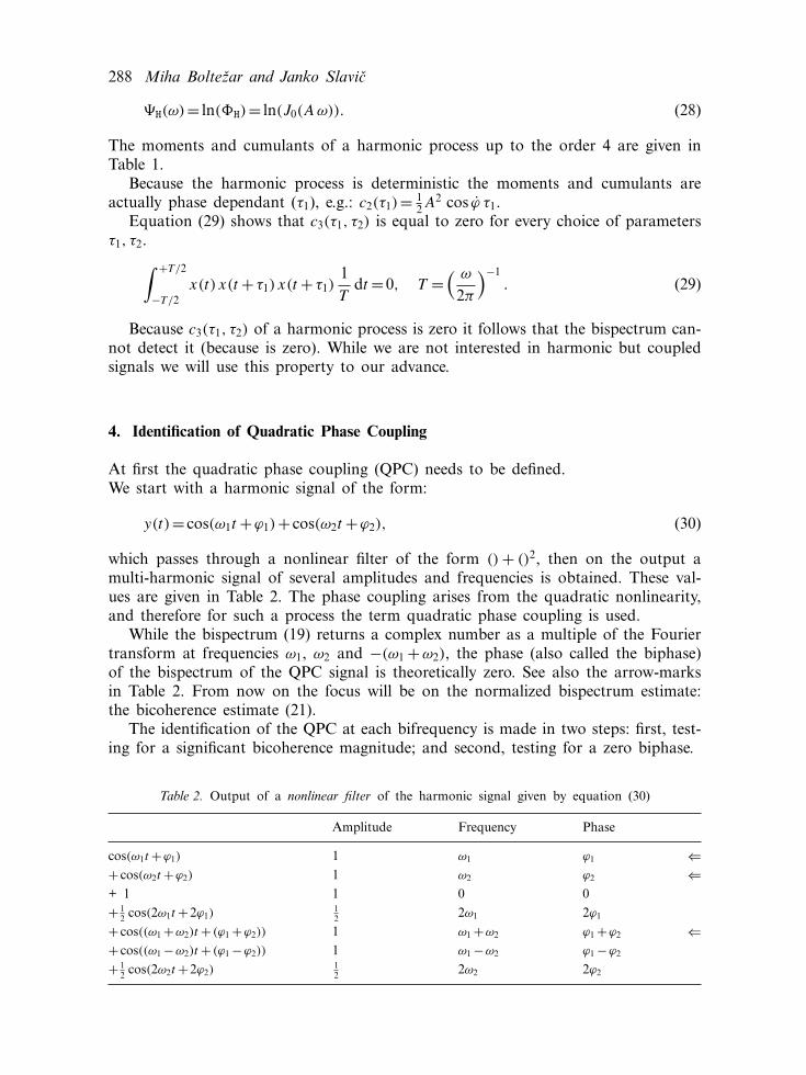
At first the quadratic phase coupling (QPC) needs to be defined.We start with a harmonic signal of the form:

y(t)= cos(ω1t +ϕ1)+ cos(ω2t +ϕ2), (30)

which passes through a nonlinear filter of the form () + ()2, then on the output amulti-harmonic signal of several amplitudes and frequencies is obtained. These val-ues are given in Table 2. The phase coupling arises from the quadratic nonlinearity,and therefore for such a process the term quadratic phase coupling is used.

While the bispectrum (19) returns a complex number as a multiple of the Fouriertransform at frequencies ω1, ω2 and −(ω1 +ω2), the phase (also called the biphase)of the bispectrum of the QPC signal is theoretically zero. See also the arrow-marksin Table 2. From now on the focus will be on the normalized bispectrum estimate:the bicoherence estimate (21).

The identification of the QPC at each bifrequency is made in two steps: first, test-ing for a significant bicoherence magnitude; and second, testing for a zero biphase.

Table 2. Output of a nonlinear filter of the harmonic signal given by equation (30)

Amplitude Frequency Phase

cos(ω1t +ϕ1) 1 ω1 ϕ1 ⇐+ cos(ω2t +ϕ2) 1 ω2 ϕ2 ⇐+ 1 1 0 0+ 1

2 cos(2ω1t +2ϕ1)12 2ω1 2ϕ1

+ cos((ω1 +ω2)t + (ϕ1 +ϕ2)) 1 ω1 +ω2 ϕ1 +ϕ2 ⇐+ cos((ω1 −ω2)t + (ϕ1 −ϕ2)) 1 ω1 −ω2 ϕ1 −ϕ2

+ 12 cos(2ω2t +2ϕ2)

12 2ω2 2ϕ2


For the test of significant bicoherence the following hypotheses are made:

– H0: the bicoherence at this bifrequency is zero (there is just Gaussian noise),– H1: the bicoherence at this bifrequency is not zero (there is more than just Gauss-

ian noise).

If the hypothesis H0 is refused, then there might be a QPC and the procedure con-tinues with the following hypotheses:

– H0: the biphase at this bifrequency is zero,– H1: the biphase at this bifrequency is not zero.

If the H0 is accepted, then a QPC is present.Haubrich [19] stated that the distribution of a skewness function for a Gaussian

process is approximately χ2 with 2 degrees of freedom. Fackrell [3] showed that fromthis property for a given significance level α, the highest/critical bicoherence level foraccepting the zero hypothesis for bicoherence is:

b2crit =−2 ln(1−α)

dof, (31)

where dof is the degree of freedom defined as: dof =2 K, where K is the number ofsegments.

The distribution of the biphase is approximately normal [14], and the highest/critical biphase for accepting the zero hypothesis for the biphase at the significancelevel αp is [3]:

∠bcrit = αp√dof

√

1

b2−1, (32)

5. Numerical Examples

As the output of the bicoherence is highly dependent on the appropriate set ofparameters.

In this numerical example the focus is given to the appropriate number of seg-ments (parameter K) and the segment length (parameter M). Both parameters haveto follow some rules.

As real signals allways include noise, there the influence of Gaussian noise addedto the signal is studied.

5.1. The Usefulness of Noise and the Importance of the Number of Segments

A synthetic signal of one QPC component was created, see Figure 1. The syntheticsignal was re-sampled to K = 256,M = 256 (19), and the overlapping was 50%. The


0 0.12 0.25 0.37 0.50 0.62 0.75

-120

-100

-80

-60

-40

-20

00 0.12 0.25 0.37 0.50 0.62 0.75

a

b c

f [Hz]

Pow

er s

pect

rum

[dB

]

Figure 1. Power spectrum of the synthetic signal (without noise). (a) 0.1249 Hz, (b) 0.2423 Hz,(c) QPC component.

bicoherence squared b2 and the phase significance were α =αp = 0.99, see equations(31) and (32). The bicoherence estimate of the synthetic signal with added noise of20 dB (33) is shown in Figure 2. As can be seen the identification of the QPC com-ponent is successful. The triangles in the Figure 2 denote the principal domain of thebispectrum; the inter triangle is defined by equation (17) and is of primary interestin this study, for details see i.e. [3].

The noise was described by the signal-to-noise ratio (SNR) in dB:

SNR=10 log10

(var(signal)var(noise)

)

. (33)

In this study Gaussian noise is used.However, the identification of QPC on a noiseless signal fails, see Figure 3. When

testing synthetic signals for QPC we have to add noise. On real signals this, however,is not usually necessary because the noise is already present. In bispectral analysisnoise up to about 20 dB can enhance the identification.

The identification also fails if the number of segments K is small, see Figure 4. Itis advisable to use K =M [15].

0

0.98

0

0.330.66

0.98

00.250.5

0.751

0.330.66

0.33 0.66 0.98

0.33

0.660 0.33 0.66 0.98

0

0.33

0.66

f1 [Hz]

f 2 [

Hz]

f1 [Hz]

f2 [Hz]

b2

Figure 2. Bicoherence of synthetic signal with SNR = 20 dB.


0.039

0.0390.14

0.24

00.250.5

0.751

0.140.24

0.14 0.24

0.14

0.24

0.039 0.14 0.24

0.039

0.14

0.24

f1 [Hz]

f 2 [H

z]

b2

f1 [Hz]

f2 [Hz]

Figure 3. Bicoherence of synthetic signal without noise.

0.0390.14

0.24

0.0390.14

0.24

00.250.5

0.751

0.14 0.24

0.14

0.24

0.039 0.14 0.24

0.039

0.14

0.24

f1 [Hz]

f 2 [H

z]

f2 [Hz]

f1 [Hz]

b2

Figure 4. Bicoherence calculated on K =16 segments. SNR = 20 dB.

5.2. Harmonic Signals

A synthetic signal of 20 harmonic components was created:

y(t)=20

∑

i=1

Ai cos(2π fi +φi). (34)

Details are given in Table 3, see also Figure 5. From Table 3 it is clear that there aretwo QPC components: the 3rd and the 6th, where the amplitudes of the latter arevery different. Next, the signal also includes a component where only frequenciesare coupled and a component where only phases are coupled.

0 0.082 0.16 0.25 0.33 0.41 0.49

-120

-100

-80

-60

-40

-20

00 0.082 0.16 0.25 0.33 0.41 0.49

f [Hz]

Pow

er s

pect

rum

[dB

]

Figure 5. Power spectrum of the synthetic signal.


Table 3. Parameters of the harmonic function

i Ai fi [Hz] ϕi i Ai fi [Hz] ϕi

1 1 0.1050 Random [0,2π) 11 1 0.3210 Random [0,2π)

2 1 0.1525 Random [0,2π) 12 1 0.3751 Random [0,2π)

3 1 f1 +f2 =0.2575 φ1 +φ2 13 1 0.4320 Random [0,2π)

4 0.1 0.3010 Random [0,2π) 14 1 0.4670 Random [0,2π)

5 1 0.4120 Random [0,2π) 15 1 0.0510 Random [0,2π)

6 1 f2 +f4 =0.4535 φ2 +φ4 16 1 0.3410 Random [0,2π)

7 1 f1 +f4 =0.4060 Random [0,2π) 17 1 0.4880 Random [0,2π)

8 1 0.0310 φ1 +φ5 18 1 0.2310 Random [0,2π)

9 1 0.2210 Random [0,2π) 19 1 0.3710 Random [0,2π)

10 1 0.2690 Random [0,2π) 20 1 0.4110 Random [0,2π)

In this study, because of the low leakage, the Hamming window was used. Thesynthetic signal was re-sampled to K = 256,M = 256, and the overlapping was 50%.The bicoherence squared b2 and phase significance were α =αp =0.99, see equations(31) and (32).

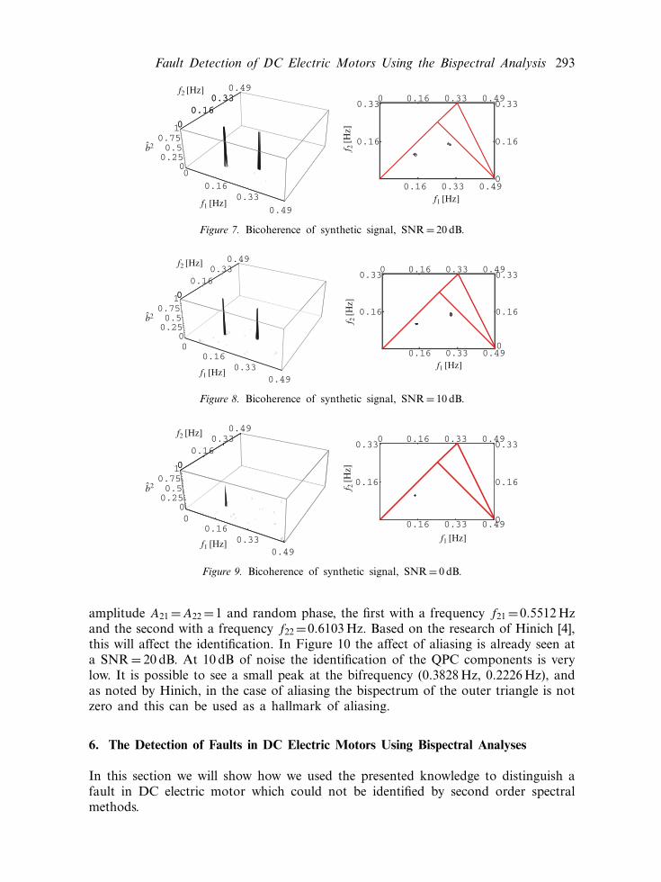
The bicoherence estimate at SNR = ∞ is given in Figure 6. It is clear thatthere are two peaks that correspond to the QPC components 3 and 6: at thebifrequency (0.1523 Hz, 0.1055 Hz) with value b2 = 0.9999 and at the bifrequen-cy (0.3008 Hz, 0.1523 Hz) with the value b2 = 0.9950. At the bifrequencies of theonly frequency-coupled component, 7, or the only phase-coupled component, 8, asexpected, there is no peak.

As the noise increases the identification of the QPC worsens, see Figures 5–9. Atabout SNR = 5 dB the QPC component 6 disappears. The reason is the very smallamplitude of one component of the QPC component 4. At about SNR = 0 dB theQPC component 3 also disappears. While 0 dB means equal variance of noise andsignal it can be stated that the QPC identification is very resistant to noise.

5.3. Harmonic Signals with Aliasing

To test the aliasing resistance of the presented methods an additional signal was cre-ated: to the previous signal two components were added. Both components had an

00.16

0.33

0.49

0

0.160.330.49

00.250.5

0.751

0.16 0.33 0.49

0.16

0.330 0.16 0.33 0.49

0

0.16

0.33

f1 [Hz]f1 [Hz]

f2 [Hz]

f 2 [H

z]

b2

Figure 6. Bicoherence of synthetic signal, SNR = ∞ dB.


0

0.160.33

0.49

0

0.160.33

0.49

00.250.5

0.7510

0.160.33

0.16 0.33 0.49

0.16

0.330 0.16 0.33 0.49

0

0.16

0.33

f1 [Hz] f1 [Hz]

f 2 [H

z]

f2 [Hz]

b2

Figure 7. Bicoherence of synthetic signal, SNR = 20 dB.

00.16

0.330.49

0

0.160.33

0.49

00.250.5

0.7510

0.16 0.33 0.49

0.16

0.330 0.16 0.33 0.49

0

0.16

0.33

f1 [Hz]f1 [Hz]

f2 [Hz]

f 2 [H

z]

b2


00.16

0.330.49

0

0.160.33

0.49

00.250.5

0.7510

0.16 0.33 0.49

0.16

0.330 0.16 0.33 0.49

0

0.16

0.33

f1 [Hz]f1 [Hz]

f2 [Hz]

f 2 [H

z]

b2


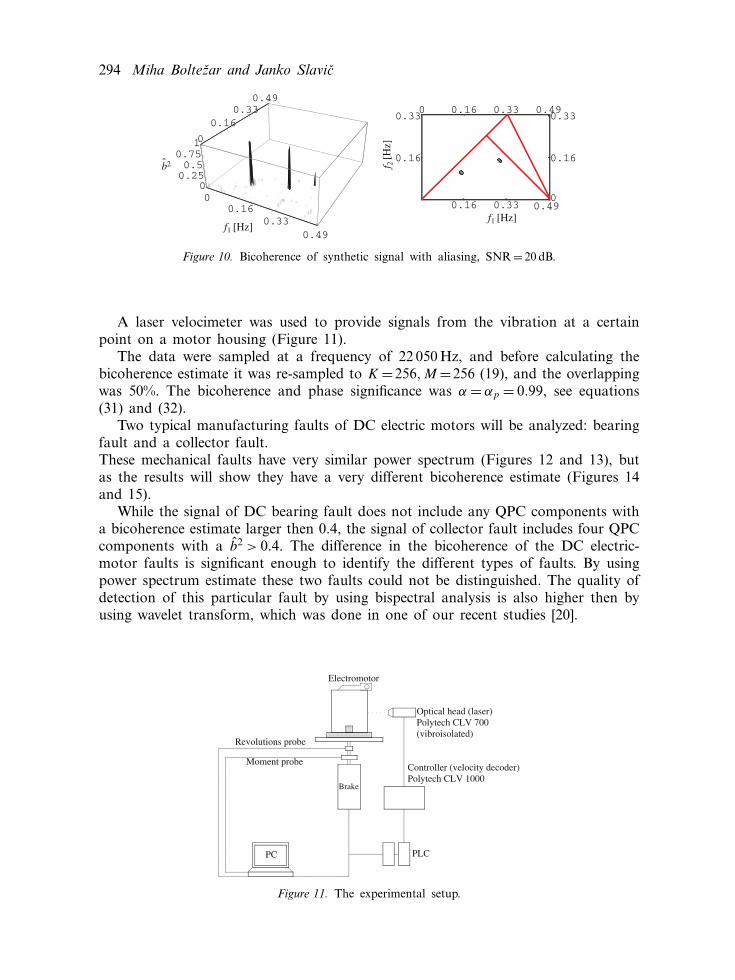
amplitude A21 =A22 =1 and random phase, the first with a frequency f21 =0.5512 Hzand the second with a frequency f22 =0.6103 Hz. Based on the research of Hinich [4],this will affect the identification. In Figure 10 the affect of aliasing is already seen ata SNR = 20 dB. At 10 dB of noise the identification of the QPC components is verylow. It is possible to see a small peak at the bifrequency (0.3828 Hz, 0.2226 Hz), andas noted by Hinich, in the case of aliasing the bispectrum of the outer triangle is notzero and this can be used as a hallmark of aliasing.

6. The Detection of Faults in DC Electric Motors Using Bispectral Analyses

In this section we will show how we used the presented knowledge to distinguish afault in DC electric motor which could not be identified by second order spectralmethods.


00.16

0.330.49

0

0.160.33

0.49

00.250.5

0.751

0.16 0.33 0.49

0.16

0.330 0.16 0.33 0.49

0

0.16

0.33

f1 [Hz]f1 [Hz]

f 2 [H

z]

b2

Figure 10. Bicoherence of synthetic signal with aliasing, SNR = 20 dB.

A laser velocimeter was used to provide signals from the vibration at a certainpoint on a motor housing (Figure 11).

The data were sampled at a frequency of 22 050 Hz, and before calculating thebicoherence estimate it was re-sampled to K =256,M =256 (19), and the overlappingwas 50%. The bicoherence and phase significance was α = αp = 0.99, see equations(31) and (32).

Two typical manufacturing faults of DC electric motors will be analyzed: bearingfault and a collector fault.These mechanical faults have very similar power spectrum (Figures 12 and 13), butas the results will show they have a very different bicoherence estimate (Figures 14and 15).

While the signal of DC bearing fault does not include any QPC components witha bicoherence estimate larger then 0.4, the signal of collector fault includes four QPCcomponents with a b2 > 0.4. The difference in the bicoherence of the DC electric-motor faults is significant enough to identify the different types of faults. By usingpower spectrum estimate these two faults could not be distinguished. The quality ofdetection of this particular fault by using bispectral analysis is also higher then byusing wavelet transform, which was done in one of our recent studies [20].

Brake

.......

.......

................

.......

.......

................

.......

.......

................

...............................................................................................................................................................................................................................................................................................................................................................................

Moment probe...................................................................................................................................................................................................................................................................................................................................................................................................................................................

..................................................................................................................................................................................................................................................................................................................................................................................................................Revolutions probe

...................................................................................................................................................................................................................................................................................................................................................................................................................................................................................................................

..

..............................................................................................................................................................................................................................................................................................................

..

..

...................................................

....................

................................................................................................................................................................

.............................................

Electromotor

........................................................................................................................................................................................................................................................................................................................................................................................................

............................................................................................................................................................

PC ........................................................................................................... ............... PLC

.......

.......

.......

.......

.......

.......

.......

.......

.......

.......

.......

.......

.......

.......

.......

..

Controller (velocity decoder)Polytech CLV 1000

.......

.......

.......

.......

.......

.......

.......

.......

.......

.......

.......

.......

.......

.......

.......

.......

.......

.......

.......

.......

.......

.......

.......

.......

.......

.......

.......

.......

.......

.......

.......

....................

..................................... Optical head (laser)

Polytech CLV 700(vibroisolated)

Figure 11. The experimental setup.


0 1809 3618 5426 7235 9044 10853

-100

-80

-60

-40

-20

00 1809 3618 5426 7235 9044 10853

f [Hz]

Pow

er s

pect

rum

[dB

]

Figure 12. Power spectrum of bearing fault.

0 1809 3618 5426 7235 9044 10853

-100

-80

-60

-40

-20

00 1809 3618 5426 7235 9044 10853

f [Hz]

Pow

er s

pect

rum

[dB

]

Figure 13. Power spectrum of collector fault.

0

36187235

10853

0

36187235

10853

00.250.5

0.7510

3618 7235 10853

3618

72350 3618 7235 10853

0

3618

7235

f1 [Hz] f1 [Hz]

f 2 [H

z]

f2 [Hz]

b2

Figure 14. Bicoherence of bearing fault.

7. Conclusions

A short overview of bispectral analysis has been presented. An important advantageof the use of cumulants is that the cumulant of the sum of independent processes isthe sum of the cumulants. While the cumulants of harmonic and Gaussian processesare zero the bispectrum cannot detect such processes. This property is used in iden-tification of QPC signals.


0

36187235

10853

0

36187235

10853

00.250.5

0.751

3618 7235 10853

3618

72350 3618 7235 10853

0

3618

7235

f1 [Hz]f1 [Hz]

f2 [Hz]

f 2 [H

z]

b2

Figure 15. Bicoherence of collector fault.

A numerical example showed that added noise can be used for a better identifica-tion of QPC and that a suitable number of segments is required for a successful iden-tification of a process. Using a numerical example it was also shown that up to 5 dBof signal-to-noise ratio the identification of QPC signals is successful, but then rap-idly worsens as the noise increases. The numerical experiment showed that the pro-cedures are also blind for harmonic components, even if they are frequency or phasecoupled.

While the identification of QPC signals is resistant to noise it is quite sensitive toaliasing. But as Hinich [4] showed, the outer triangle of the bispectrum can be usedfor identifying the presence of aliasing, and as a consequence, it can be avoided.

Data from a real experiment was used to demonstrate the ability of the bicoher-ence estimate in condition monitoring to identify different types of manufacturingfaults in DC electric motors. As an example, two typical faults with different mechan-ical causes, but with very similar power spectrum, were analyzed. Their bicoherenceestimates differ from each other significantly, and represent a good identificationbase.

References

1. Boltezar, M. and Hammond, J.K., ‘Experimental study of the vibrational behaviour of a couplednon-linear mechanical system’, Mech. Syst. Signal Proce. 13(3) (1999) 375–394.

2. Hinich, M.J., ‘Testing for gaussianity and linearity of a stationary time series’, J. Time Ser. Anal.3(3) (1982) 169–176.

3. Fackrell, J.W.A., Bispectral Analysis of Speech Signals. PhD thesis, The University of Edinburgh,UK, 1996.

4. Hinich, M.J. and Wolinsky, M.A., ‘A test for aliasing using bispectral analysis’, J. Am. Statist.Assoc. 83(402) (June 1988) 499–502.

5. Zhang, G.C., Ge, M., Tong, H., Xu, Y. and Du, R., ‘Bispectral analysis for on-line monitoringof stamping operation’, Eng. Appl. Artif. Intel. 15(1) (Februar 2002) 97–104.

6. Yang, D.M., Stronach, A.F. and MacConnell, P., ‘The application of advanced signal processingtechniques to induction motor bearing condition diagnosis’, Meccanica 38(2) (2003) 297–308.

7. Wang, W.J., Wu, Z.T. and Chen, J., ‘Fault identification in rotating machinery using the corre-lation dimension and bispectra’, Nonlinear Dynam. 25(4) (August 2001) 383–393.

8. Kocur, D. and Stanko, R., ‘Order bispectrum: a new tool for reciprocated machine conditionmonitoring’, Mech. Syst. Signal Proce. 16(2–3) (Mar–May 2002) 391–411.

9. Jeffries, W.Q., Chambers, J.A. and Infield, D.G., ‘Experience with bicoherence of electrical powerfor condition monitoring of wind turbine blades’, IEE proce. Image signal proces 145(3) (Jun1998) 141–148.


10. Simonovski, I., Boltezar, M., Gradisek, J., Govekar, E., Grabec, I. and Kuhelj, A., ‘Bispectralanalysis of the cutting process’, Mech. Syst. Signal Proce. 16(6) (2002) 1111–1122.

11. Boltezar, M., Jaksic, N., Simonovski, I. and Kuhelj, A., ‘Dynamical behaviour of the planar non-linear mechanical system – Part II: experiment’, J. Sound Vib. 226(5) (October 1999) 941–953.

12. Jaksic, N., Boltezar, M., Simonovski, I. and Kuhelj, A., ‘Dynamical behaviour of the planar non-linear mechanical system – Part I: theoretical modelling’, J. Sound Vib. 226(5) (October 1999)923–940.

13. Simonovski, I., Uporaba spektrov tretjega reda pri analizi nelinearnih mehanskih nihanj (ThirdOrder Spectra to the Analysis of Nonlinear Dynamical Systems). Master’s thesis, Fakulteta zastrojnistvo, Univerza v Ljubljani, 1998. In Slovene.

14. Elgar, S. and Sebert, G., ‘Statistics of Bicoherence and Biphase’, J. Geophys. Res. 94(C8) (August1989) 10993–10998.

15. Chandran, V. and Elgar, S., ‘Mean and variance of estimates of the bispectum of a har-monic random process – an analysis including leakage effect’, IEEE Trans. Signals Proce. 39(12)(December 1991) 2640–2651, citeseer.nj.nec.com/207643.html.

16. Nikias, C.L. and Petropulu, A.P., Higher-order Spectral Analysis, Prentice-Hall, Inc., 1993.17. Simonovski, I., Boltezar, M. and Kuhelj, A., ‘Osnove bispektralne analize (Theoretical Back-

ground of the Bispectral Analysis)’, Strojniski Vestnik-J. Mech. Eng. 45(1) (1999) 12–24.18. Newland, D.E., An Introduction To Random Vibrations, Spectral And Wavelet Analysis, 3rd edn,

Addison Wesley Longman Limited, 1993.19. Haubrich, R.A., Earth Noise, 5–500 Milicycles per second’, J. Geophys. Res. 70(6) (March 1965)

1415–1427.20. Boltezar, M., Simonovski, I. and Furlan, M., ‘Fault detection in DC electro motors using the

continuous wavelet transform’, Meccanica 38(2) (2003) 251–264.

fault detection of dc electric motors using the …lab.fs.uni-lj.si/ladisk/data/pdf/fault detection...

Documents