A Variant of Cyclic Pursuit for Target Tracking Applications:

Theory and Implementation

Sangeeta Daingade Arpita Sinha Aseem Vivek Borkar Hemendra Arya

Accepted: 03 August 2015

Abstract

This paper presents a variant of the cyclic pursuitstrategy that can be used for target tracking appli-cations. Cyclic pursuit has been extensively used inmulti-agent systems for a variety of applications. Inorder to monitor a target point or to track a slowlymoving vehicle, we propose to use a group of non-holonomic vehicles. At equilibrium, the vehicles forma rigid polygonal around the target while encirclingit. Necessary conditions for the existence of equilib-rium and the stability of equilibrium formations areanalysed consider unicycle model of the vehicles. Thestrategy is then applied to miniature aerial vehicles(MAV) represented by 6-DOF dynamical model. Fi-nally the results are verified in a Hardware In-LoopSimulator in real time, which included all on-boardelectronics of the MAVs.

Cyclic pursuit, target tracking micro aerial vehiclesmulti-agent system cooperative control hardware-in-loop simulation

1 Introduction

Multi-vehicle systems are found suitable in many ap-plications as compared to single vehicle system dueto the various advantages like better reliability, scal-ability, efficiency, operational capability, adaptabil-ity, etc. Greater benefits can be derived from suchsystems if the vehicles work in cooperation. In co-operative control, the objective is to design controlstrategies for such multi-agent systems in order toenable them to work in cooperation towards common

desired objectives. The various research areas in co-operative control are consensus, formation control,distributed task assignment and distributed estima-tion (refer Cao et al.[1] and references therein). Thiswork addresses the cooperative control problem formonitoring a target with multiple autonomous vehi-cles.

1.1 Previous work

In various military and civil applications such assurveillance, security systems, space and under wa-ter exploration, it is often required to track a targetmoving in a dynamic environment. In such situa-tions, cooperative target tracking with simple multi-ple agents could be a better solution than employing asingle, intelligent and sophisticated vehicle. In coop-erative target monitoring, the objective is to coordi-nate the motion of vehicles so that they reach the de-sired relative positions and orientations with respectto the target and maintain this formation as they fol-low the target. Kobayashi et al. [2] have proposeda decentralised control scheme for target capturingby multiple linear agents based on gradient descentmethod. Guo et al. [3] studied the formation of groupof robots enclosing a moving target where the inter-action topology may change as the system evolves.In [4], Kim and Sugie have proposed a distributedapproach based on a modified cyclic pursuit strat-egy to achieve a target-capturing task in a 3D space.In [5] Ma and Hovakimyan have developed controllaws for both single-integrator and double-integratorrobot models and have assumed that the robots haveinformation about target’s position, velocity, and ac-

1

celeration. The target tracking strategies discussedby Kobayashi et al. [2] , Guo et al. [3] , Kim andSugie [4] , Ma and Hovakimyan [5] , are applied toagents represented by linear models.The target tracking strategies discussed by Paley

et al. [6], Napora and Paley[7], Klein and Morgansen[8], Klein et al. [9], Ceccarelli et al. [10], Kingstonand Beard [11], Lan et al. [13], Lan et al. [14],Kothari et al. [15] are based on unicycle model andassume that all the agents are homogeneous. Theunicycle model closely resembles the dynamics of mo-bile robots and unmanned aerial vehicles (UAVs).Paley et al. [6] have designed switching control law totrack the centre of mass of the agents. The authorsin [7], have designed an observer based feedback con-trol for stabilisation of multiple vehicles where eachvehicle needs relative position and relative velocityinformation of neighbouring vehicles. In [8] and [9]Klein et al. have studied target tracking using threeagents and assuming full information about of thetarget as well as all other agents. These results areextended to 3D space in [9]. The strategy discussedby Ceccarelli et al. [10], allows the agents to get dis-tributed around the target in different platoons andnot necessarily be uniformly distributed along thecircle. The splay state configuration introduced byKingston and Beard in [11] enables representation ofthe equilibrium state of the agents tracking a movingtarget. The control law used here requires knowledgeof the derivative of the heading angle which mightnot always be known or computed with precision. In[12], only range and range-rate information is usedto encircle a target using multiple UAVS. The con-trol law designed by Lan et al. [13] [14] for targetenclosing switches between several possibilities, firstto bring the vehicles near the target and then to co-ordinate their motion to achieve uniform distributionaround the target. In [13], Lan et al. have proposeda state-dependent hybrid controller to steer the vehi-cles closer to the target and then coordinate their mo-tion to achieve evenly spaced circular motion aroundthe fixed target. Lan et al. have designed a switch-ing control law in [14] based on reachability and in-variance analysis to achieve independent motion to-wards the target without any inter-vehicle interactionwhen the vehicles are far away from the target and

a coordinated motion when they are near the target.Kothari et al. [15] proposed a sliding mode controlleralong with consensus protocol to maintain a fixed rel-ative position of a group of UAVs with respect to amoving target. Chen and Zhang [16] have proposeda leader-free no-beacon decentralised algorithm forgenerating a collective circular motion. Moshtagh etal. [17] have proposed a vision based control law forachieving circular formation which needs only bear-ing angle information of the neighbours. With thestrategies discussed in [16] and [17], the agents fi-nally converge to a circular formation but the pointabout which the formation converges cannot be spec-ified a priori. In order to enable target enclosing weshould be able to achieve formations about a specificpoint (target). Ground vehicle tracking using mul-tiple UAVs considering vision input is discussed inMa and Hovakimyan [18] where the target trackingcontrol and coordination control are designed sepa-rately. For tracking control both bearing angle andrange measurements are required whereas the coordi-nation term in the control law is a nonlinear functionof the bearing angle.The papers by Bakolas and Tsiotras [19], Olfati-

Sabar and Sandell [20], Petitti et al. [21] study targettracking from a different perspective. Relay pursuitbased target tracking strategy proposed in [19] as-signs the task of capturing a manoeuvring target toonly one of the agents and this assignment can changedynamically with time according to a proximity re-lation. During the pursuit, other agents remain sta-tionary. So here the objective is to only track thetarget and not to maintain the formation. In [20]and [21], target tracking is defined with the objectiveto estimate the position information about the tar-get using distributed sensory agents. In Petitti et al.[21] the authors have presented consensus based dis-tributed target tracking algorithm, where they haveconsidered sensor network of heterogeneous agents toestimate the target position.The work presented in this paper is based on cyclic

pursuit which is a simple strategy derived from thebehaviour of social insects. In cyclic pursuit, agenti follows agent i + 1 modulo n. This strategy canbe used to obtain various behaviours like rendezvous,circular motion, spiralling motion etc. Bruckstein et

2

al. [22] have modelled behaviours of ants, cricketsand frogs with continuous and discrete cyclic pursuitlaws. Stability and convergence of group of ants inlinear pursuit have been described in [23] by Bruck-stein. Sinha and Ghosh [24] have proposed a general-ization of the linear cyclic pursuit law with the appli-cation to rendezvous of multiple agents having differ-ent gains. In [25], the formations of multiple unicycletype agents in cyclic pursuit have been studied whereat equilibrium the agents converge to circular forma-tions about a point depending on initial positions ofthe agents. Sinha and Ghosh [26] have studied gen-eralised nonlinear cyclic pursuit and derived a neces-sary condition for equilibrium formation of heteroge-neous agents. Rattan and Ghosh [27] have proposedImplicit Leader Cyclic Pursuit (ILCP) law for achiev-ing formations about a given goal point and have usedit for rendezvous of multiple vehicles. In this strategyone of the agent is the implicit leader who knows theposition of the target and drives the formation to-wards it. Remirez-Riberos et al. [30] have proposeda cyclic pursuit based strategy for single integratorand double integrator type agents to achieve circularformation about a specific point and have applied thesame to control nonholonomic robots using feedbacklinearization. Besides these there are different strate-gies addressed in the literature based on cyclic pur-suit to achieve various formation patterns as given inPavone and Frazzoli [28], Ramirez [29] and Gallowayet al. [31] to list a few.

1.2 Contribution

In this paper, we present a variant of the cyclic pur-suit strategy for target tracking applications usingnon-holonomic vehicles. Cyclic pursuit based forma-tion control strategies discussed in [25] and [26] dealwith circular formations about a point which cannotbe specified a priori. To overcome this limitation, animplicit leader following strategy under cyclic pur-suit was proposed in [27]. We propose a decentralisedstrategy based on cyclic pursuit law that can achievethe formation of the agents around the target point.The agents have unicycle kinematics. They can beidentical, in which case, we will have homogeneousgroup of agents. We can also have heterogeneous

group of agents. We assume that the target track-ing is achieved if 1) the agents move on circles withthe target at the centre and 2) the agents are alwaysuniformly located around the target. In case of homo-geneous agents, a uniform formation will be achievedif the angle separation between adjacent agents withrespect to the target is equal for all agents. We de-fine this strategy as Target Centric Cyclic Pursuit(TCCP). The novelty of this work lies in derivinga simple control strategy which can be easily mea-sured and computed and can be conveniently imple-mented on actual hardware. We have analysed theformation of the agents about a stationary target andvalidated the result on 6DOF model of UAVs andon Hardware-in-loop-simulator (HILS) of the microaerial vehicle. Extensive simulations have been car-ried out to test different conditions like tracking amoving target, the effect of wind on the formationand the effect of changing the frequency of informa-tion updates on the formation. Preliminary resultsare presented in [32], [33].This paper is organised as follows. The system is

modelled in Section 2 followed by possible equilib-rium formations in Section 3. Stability analysis ofequilibrium formations for homogeneous agents arestudied in Section 4. We extended the strategy to all-to-all communication in Section 5. Section 6 gives therealistic MAV model and the details of control imple-mentations on the autopilot. Implementation of thisstrategy on Hardware-In-Loop Simulator is discussedin 7. Simulation results and conclusions are presentedin Sec 8 and 9 respectively.

2 Problem Formulation

Consider a group of n agents employed to track atarget. The kinematics of each agent with a singlenonholonomic constraint can be modeled as:

xi = Vi cos(hi), yi = Vi sin(hi), hi = ui =aiVi

= ωi

(1)where Pi ≡ [xi, yi]

T represents the position of agent i,hi represents the heading angle of the agent i with re-spect to a global reference frame and Vi and ai repre-sent the linear speed and lateral acceleration of agent

3

Ref.P

Pi

Pi+1

P′

i+1

f i+1i

fi

δ

hi

hi+1

zi

φi

Y

X

rig

ri

r′

i

ρr(i+1)g

Vi+1

Vi

Figure 1: Positions of the vehicles in a target centricframe

i. Equation (1) can represent a point mass model of aUAV flying at a fixed altitude or a point mass modelof a wheeled robot on a plane. We use a generic term“agent” to represent the aerial or ground vehicle. Weassume that the agent i is moving with constant lin-ear speed, that is Vi is constant and the motion of theagent i is controlled using the lateral acceleration, ai.

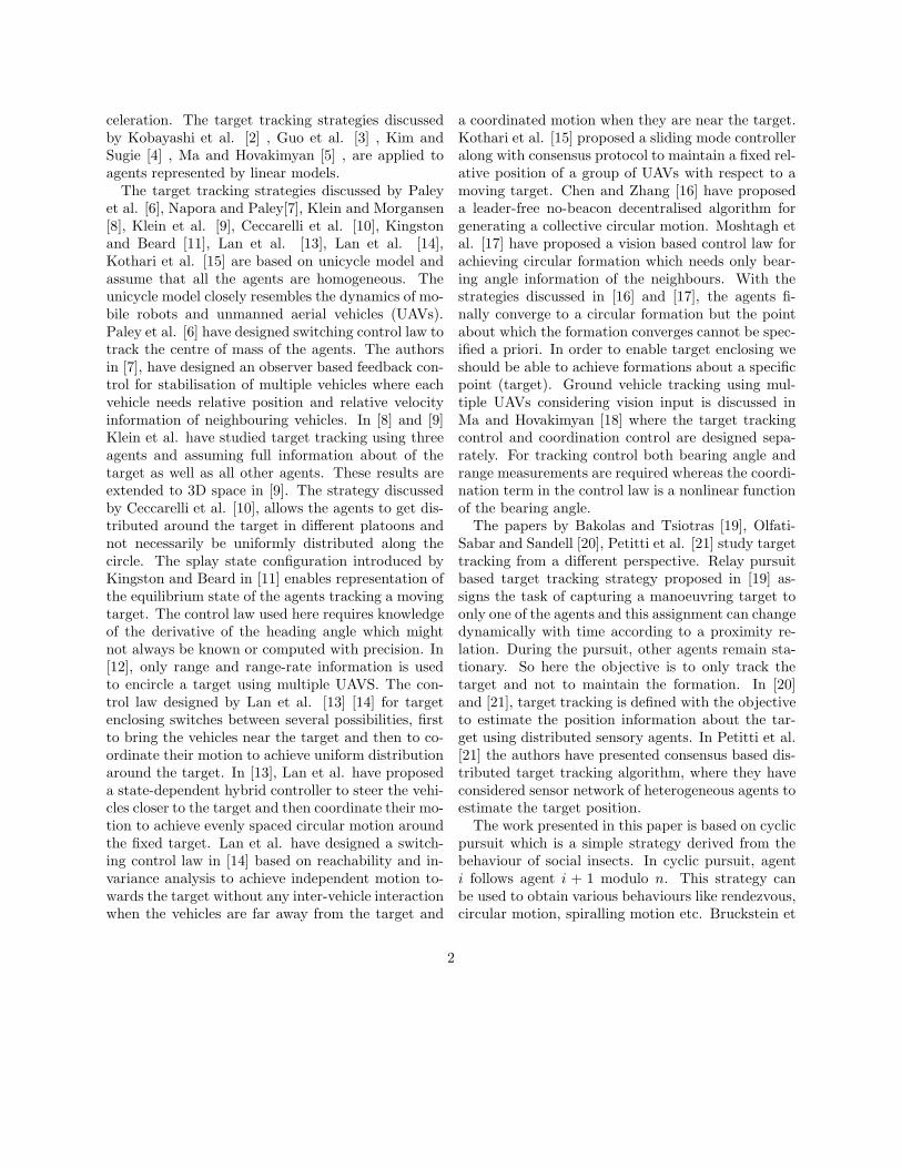
Our objective is to enclose the target with n agents.The target is stationary. It is assumed that eachagent i has the information about the target posi-tion and i+1th agent’s position. Consider the targetto be located at point P as shown in Fig. 1. Wemodify the classical cyclic pursuit law for target en-closing problem such that agent i, positioned at Pi,follows not only i + 1th agent at Pi+1 but also thetarget at P . Let ρ be a constant, which decides theweight agent i gives to the target position P , overthe position of the agent i + 1, Pi+1. This weighingscheme is mathematically equivalent to following avirtual leader located at the point P

′

i+1 which is a

convex combination of P and Pi+1. The point P′

i+1

is calculated as P′

i+1 = ρ Pi+1 + (1 − ρ) P , where

0 < ρ < 1. The parameter ρ is called the pursuit

gain. We consider a target centric reference frame asshown in Fig. 1. The variables in Fig. 1 are:rig – Distance between ith agent and the target,ri – Distance between ith agent and i+ 1th agentri

′

– Distance between ith agent and virtual leaderat P

′

i+1,fi – angle made by the vector rig w.r.t referenceφi – angle between the heading of ith agent and mod-ified LOS PiP

′

i+1.We define the control input to the ith agent as

ui = kiφi (2)

where, ki > 0 is the controller gain. We assumethat φi(t) ∈ [0, 2π) for all time, t ≥ 0. This condi-tion ensures that the agents always rotate in counterclockwise direction. Also lateral acceleration remainsbounded for a fixed ki. Let us define the states of thesystem as

xi(1) = rig, xi(2) = f i+1i , xi(3) = hi − fi (3)

for i = 1, 2, · · ·n. Then the kinematics (1) can bere-written in the target centric reference frame as,

xi(1) = Vi cos(xi(3)) (4a)

xi(2) =Vi+1 sin(xi+1(3))

xi+1(1)− Vi sin(xi(3))

xi(1)(4b)

xi(3) = kiφi −Vi sin(xi(3))

xi(1). (4c)

In practical situation, the agents will have a limit onthe maximum lateral acceleration amax, that is, ai ≤amax∀i. We can take into account this constraintby imposing an upper bound on the value of ki as,ki ≤ kmax where kmax = amax

2πVi.

3 Formation at equilibrium

We study the asymptotic behavior of a group ofheterogeneous agents under the control law (2).

Consider n agents with kinematics (4). Atequilibrium, the agents move on concentric circles,with (i) the target at the center of concentric

4

circles and (ii) equal angular velocities. Atequilibrium xi(j) = 0 for i = 1, ..., n and j = 1, 2, 3.So the distance between the target and agent,rig for all i, remains constant at equilibrium.From (4a) hi − fi = (2m + 1)π2 for all i, wherem = 0,±1,±2, · · · . Substituting this value in (4c)

we get kiφi = Vi sin(hi−fi)rig

= ± Vi

rig. Since φi ≥ 0,

ki > 0, Vi > 0 and rig ≥ 0, we can write

kiφi =Virig

(5)

and therefore, m = 0,±2,±4, · · · . Assuming hi ∈[0, 2π) and fi ∈ [0, 2π), we get (hi − fi) ∈ (−2π, 2π).So m = 0 or m = −2. From geometry, m = 0 andm = −2 implies the same angle. Therefore hi − fi =π2 . From (2) and (5), ui = ωi =

Vi

rig. Since Vi and rig

are constant, ωi is constant for all i. Therefore all theagents move along a circular path with the target atthe center and radius rig. This proves the first partof the theorem.The angular velocity of agent i can be calculated as,ωi = hi − fi = Vi

rig. As hi − fi = π

2 from equation

(4b)Virig

=Vi+1

r(i+1)g(6)

for all i. Hence we conclude that, for all i, ωi = ωi+1.Therefore, all the agents move around the target inconcentric circles with equal angular speed. Considern agents with kinematics (4). At equilibrium, theagents form a rigid polygon that rotates about thetarget. The proof follows directly from Theorem 3.Next we derive necessary conditions for the existenceof equilibrium. Consider Fig. 1. Let ∠PP

′

i+1Pi = ziand f i+1

i = fi+1 − fi. Let us define a set of agentsX as, X =

{

i : ρ < Vi

Vi+1, i ∈ {1, · · · , n}

}

.

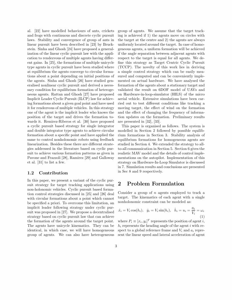
The set X 6= ∅. We prove it by contradic-tion. Let us assume that X = ∅. Then ρVi+1 ≥ Vifor all i = 1, · · · , n (mod n), which implies,ρnV1 ≥ V1. But this can not be true since 0 < ρ < 1.So there exits at least one agent in the set X .For the agents in set X , from (6), ρr(i+1)g < rig.Now, consider an agent i ∈ X . Fig. 2 shows thetrajectory of agent i at equilibrium, with respect to

P

Q′

Q

rig

ρr(i+1)g

Q0

Vi

φimax

φ′

Pi

φiminQ2

Figure 2: Formation of agents in set X

the target located at point P . The agent i movesalong the circle which has radius rig and center P .Let the agent i be at the point Pi. For a given ρ,the virtual leader of agent i will lie on the circleof radius ρr(i+1)g which is less than rig . Note thatr(i+1)g can be greater or less than rig . Let PiQand PiQ

′ be the tangents drawn from point Pi tothe inner circle of radius ρr(i+1)g and φimin

and

φimaxare the angles that the velocity vector of ith

agent makes with PiQ and PiQ′ respectively. Then,

φimin+φimax

= π. At equilibrium, φi ∈ [φimin, φimax

]When φi = φimin

, the virtual leader of i will beat Q and therefore f i+1

i = φi. Similarly, when

φi = φimax, f i+1

i = π + φi. When φi = φ′

which iswithin the bounds, there are two possible locationswhere the virtual leader can lie (Q1 and Q2). So zican take two values, zia = ∠PQ1Pi = z

′

i (say) andzib = ∠PQ2Pi = π − zi

′. Using (6) and sine rule for4PQ1Pi, we get

z′

i = sin−1

(

ViρVi+1

cosφi

)

. (7)

Similarly, f i+1i can take two values. At equilibrium,

right hand side of (7) should be real. So the neces-sary condition for the existence of equilibrium canbe stated as:

5

Consider n agent system with kinematics (4).Given ρ, the necessary condition for equilibrium is

maxi∈X

ηi ≤ minj∈X

µj (8)

ηi =kiV1

cos−1(ρVi+1

Vi

)

(9a)

µj =(

π − cos−1(ρVj+1

Vj

)) kjV1. (9b)

For i /∈ X , i.e. if ρVi+1 ≥ Vi, RHS of equation (7)is always real. However, if i ∈ X , then we shouldhave

φi ∈[

pπ + cos−1(ρVi+1

Vi

)

, (p+ 1)π − cos−1(ρVi+1

Vi

)]

(10)where, p = 0,±1,±2, · · · . As φi ∈ [φimin

, φimax] ⊆

[0, π], p can take only one value, p = 0. Let the radiusof the circle traversed by the first agent r1g = R1.Then from (5) and (6),

φi =V1kiR1

. (11)

Using (10) and (11) for a given i ∈ X we can write,ηi ≤ 1/R1 ≤ µi, where ηi and µi are as given in (9).Let

<i = {R1 : ηi ≤ 1/R1 ≤ µi, i ∈ X}. (12)

If⋂

i∈X <i 6= ∅ then there exists some R1 such thatRHS of (7) is real ∀i ∈ X . For this to be true, (8)must hold. So the necessary condition for equilib-rium is given by (8). For the agents not in set X ,that is, ρVi+1 ≥ Vi, from (6), ρr(i+1)g ≥ rig . Whenρr(i+1)g = rig , the virtual leader lies on the circleof radius rig and φi can take value in [0, π]. Whenρr(i+1)g > rig, the virtual leader lies outside the cir-cle of radius rig and φi ∈ [0, 2π). In both the cases,given a φi, there exists an unique point where vir-tual leader can lie and hence the position of the nextagent i+ 1 is unique. In these cases, we always havezi = z

′

i.Even if a system of n agents satisfy Theorem 3 they

may not satisfy

n∑

i=1(mod n)

(f i+1i ) = 2πd, d = ±1,±2, · · · . (13)

Therefore, to achieve a formation, one requires bothTheorem 3 and (13) to be true simultaneously.

4 Formation in case of homoge-neous agents

Consider the case when all the agents are identical.We study this case in detail since in multi agent re-search often we are interested in multiple identicalagents that are easily scalable. As the agents areidentical, Vi = V and ki = k, ∀i. Then at equilib-rium, from (6) we have rig = R, ∀i. So the agentsmove on the same circle with the target at its cen-ter. From (11), φi = V

kR= φeq for all i, and from

4PPiP′

i+1 in Fig. 1,

cos(φeq) =ρ sin(f i+1

i )√

1 + ρ2 − 2ρ cos(f i+1i )

. (14)

We observe that ρV < V and therefore all the agentsbelong to the set X . From Fig. 2, for 4PQPi, ρ =cos(φmin). Assuming φ

′

= φeq , ∠Q0PPi = φeq . Let∠Q0PQ1 = ∠Q0PQ2 = δ,

fa = ∠PiPQ1 = φeq + δ (15)

fb = ∠PiPQ2 = φeq − δ. (16)

f i+1i can be either fa or fb. As long as φeq ∈[φmin, φmax], Theorem 3 is trivially satisfied. From4Q1PPi,

cos(φeq) = ρ cos(δ). (17)

Let, at equilibrium, Ma = {i : f i+1i = fa} and Mb =

{i : f i+1i = fb}. Then |Ma| + |Mb| = n. We have

three possibilities:WhenMa is empty, that is, f i+1

i = fb = φeq−δ ∀i,cos(fb) = cos(φeq − δ). Using (14) and (17), aftermathematical manipulations we get, 2

(

ρ cos(fb) −1)(

ρ− cos(fb))

= 0. Since, 0 < ρ < 1, ρ cos(fb) 6= 1.So ρ = cos(fb). Since ρ = cos(φmin), either fb =φmin or fb = 2π− φmin = π+φmax. Then from Fig.2, we observe that the agent i+ 1 will be at Q or Q′

and thus we have either φeq = φmin or φeq = φmax.When Mb is empty, that is, f i+1

i = fa ∀i,cos(fa) = cos(φeq + δ). Then following similar proce-dure as in the previous case we get ρ sin2(fa)−

(

1−

6

ρ cos(fa))(

ρ−cos(fa))

= cos(fa)(

1+ρ2−2ρ cos(fa))

.This equation is trivially satisfied for all ρ.When both Ma and Mb are non-empty, following

similar procedure, it is found that the equilibriumformation is possible if cos(δ) = ρ cos

(

2π dn− m

nδ)

istrue for the values of δ satisfying cos(φeq) = ρ cos(δ)and m = |Ma| − |Mb|.For Cases 1 and 2, we have f i+1

i = f ∀i, wheref is some constant. However, in Case 3, f i+1

i is notsame for all i. A set of 40000 Monte Carlo simula-tions were run for different values of n and ρ. Thevalue of n was varied from 3 to 11 and ρ from 0.1to 0.9 in the steps of 0.1. We selected 500 randominitial conditions for each pair of n and ρ. It hasbeen observed that, formation at equilibrium was al-ways a regular polygon, which mean Case 3 has neveroccurred. Also Case 3 will not result in an uniformformation of agents around the target. So in this pa-per, we will concentrate on Cases 1 and 2 only andanalyze the conditions for achieving a stable forma-tion uniformly distributed around the target.In Case 1 and Case 2, we observe that φmin ≤ f ≤

π + φmax with Case 1 corresponding to equalities.When f i+1

i = f ∀i, the agents will be uniformlydistributed around the target. Then from (13),

f = 2πd

n. (18)

Since φeq = VkR

, the distance between an agent andthe target at equilibrium is

R =V

kφeq(19)

and the distance between ith and i+1th agent, r canbe obtained (refer to Fig. 1) as

r = 2R sin( f

2

)

= 2V

kφeqsin(π

d

n). (20)

Then the states of the system (4) at equilibrium are

xi(1) =V

kφeq, xi(2) = 2π

d

n, xi(3) =

π

2. (21)

Thus, at equilibrium, the agents arrange themselvesin a regular formation around the target. This regu-lar formation of n agents can be described by a reg-ular polygon {n

d}, where d ∈ {1, 2, ..., n− 1}. This d

−1 0 10

0.1

0.2

0.3

0.4

0.5

0.6

0.7

0.8

0.9

1

ρ −−−>

q −

−−

> I

III

II

Figure 3: q versus ρ plot when ρ = cos(2πq)

is reflected in equilibrium state xi(2) in (21).At equilibrium φmin ≤ f ≤ π + φmax. So

ρ = cos(φmin) ≥ cos(f) = cos(2π dn). Thus, ρ ≥

cos(2π dn). Let us replace d

nby a continuous variable

q ∈ (0, 1). We can plot ρ = cos(2πq) as shown inFig. 3. It can be seen that, for a given n, RegionI corresponds to Case 2 (when Mb is empty) andthe boundary of the Region I corresponds to Case 1(when Ma is empty).Next, we can study the stability of the regular polyg-onal formation of homogeneous agents obtained atequilibrium by linearizing the system of n agents (4),about the equilibrium point (21). Linearizing the sys-tem we get ˙

xi = Axi + Bxi+1. where

A =

0 0 −VVR2 0 0

kρ sin(2π dn)

R

(

1+ρ2−2ρ cos(2π dn)) + V

R2

kρ

(

ρ−cos(2π dn))

(

1+ρ2−2ρ cos(2π dn)) −k

B =

0 0 0−VR2 0 0

−kρ sin(2π dn)

R

(

1+ρ2−2ρ cos(2π dn)) 0 0

.

So, the system of n vehicles, can be written

as˙X = AX where X = [x1, x2, · · · , xn]

T

and A is a circulant matrix given by A =circ

(

A B 03×3 · · · 03×3

)

. The stability of

the formation depends on the eigenvalues of A.Consider n agents with kinematics (4). For a given

value of ρ, the equilibrium points given by (21) are

7

locally asymptotically stable if

ql <d

n< qu (22)

ql = −0.17ρ+ 0.254

qu =

{

0.17ρ+ 0.75 for ρ ≤ 0.53052πcos−1(

√2ρ− 1) for ρ > 0.5305.

(23)

The stability of a formation depends on the eigen-values of the circulant matrix A. We can find theeigenvalues of circulant matrix (as given in Davis [34]) using the representer polynomial P (z) of circulantmatrix A. The representer polynomial of a circu-lant matrix C = circ (C1, C2, · · ·Cn) is defined asP (z) =

∑n

i=1Ci(z

i−1). So the representer polyno-

mial of A will be,

P (z) = A+ zB.

Let ς = ej2πn , where j =

√−1. The block circulant

matrix A can be diagonalized using Fourier matrixFn as,

A = (Fn ⊗ I3)?D(Fn ⊗ I3),

where (?) indicates conjugate transpose.The diagonal matrix D is given by, D =diag(P (1), P (ς), · · · , P (ςn−1)). So we can writeDi = A+ ςi−1B, i ∈ {1, 2, ....n}.The eigenvalues of A are same as eigenvalues of Di,i = 1, · · ·n. So we can comment about the stabilityof n vehicle system, by observing the eigenvalues ofeach block Di. Substituting the value of R, eachDi can be factorized as Di = kT−1DiT , whereT =diag[k, V, V ] and

Di =

0 0 −1

φeq2(1− ςi−1) 0 0

φeqρ sin(2π dn)(1−ςi−1)

1+ρ2−2ρ cos(2π dn)

+ φeq2 ρ(ρ−cos(2π d

n))

1+ρ2−2ρ cos(2π dn)

−1

.

The spectrum σ(·) of Di and Di are related asσ(Di) = kσ(Di). Since k > 0 , stability of Di canbe determined from the stability of Di. As Di doesnot have a term containing gain k as well as V , we

0 0.2 0.4 0.6 0.8 10

0.1

0.2

0.3

0.4

0.5

0.6

0.7

0.8

0.9

1

ρ

q =

d /

n

I

II

III

IV

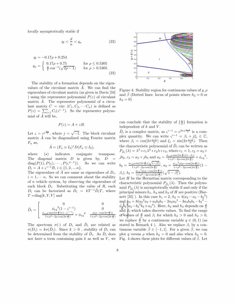
Figure 4: Stability region for continuous values of q, ρand β (Dotted lines: locus of points where h2 = 0 orh3 = 0)

can conclude that the stability of {nd} formation is

independent of k and V .

Di is a complex matrix, as ςi−1 = e2πji−1n is a com-

plex quantity. We can write ςi−1 = βi + jξi ∈ C,where βi = cos(2π i−1

n) and ξi = sin(2π i−1

n). Then

the characteristic polynomial of Di can be written asPDi

(λ) = λ3+c1λ2+c2λ+c3, where c1 = 1, c2 = a2+

jb2, c3 = a3+ jb3 and a2 =φeqρ sin(2π d

n)(1−βi)

1+ρ2−2ρ cos(2π dn)+φeq

2,

b2 =φeqρ sin(2π d

n)(√

1−β2i)

1+ρ2−2ρ cos(2π dn)

, a3 =φeq

2ρ(ρ−cos(2π dn))

1+ρ2−2ρ cos(2π dn)(1 −

βi), b3 =φeq

2ρ(ρ−cos(2π dn))

1+ρ2−2ρ cos(2π dn)(√

1− β2i ).

Let H be the Hermitian matrix corresponding to thecharacteristic polynomial PDi

(λ). Then the polyno-mial PDi

(λ) is asymptotically stable if and only if theprincipal minors h1, h2 and h3 ofH are positive (Bar-nett [35] ). In this case h1 = 2, h2 = 4(a2 − a3 − b2

2)and h3 = 8(a2

2a3+a2b2b3− 2a2a32− 3a3b2b3− b32−

a3b22a2−b23b3+a33). Here, h2 and h3 depends on d

n

and βi which takes discrete values. To find the rangeof values of d

nand βi for which h2 > 0 and h3 > 0,

we replace dnby a continuous variable q ∈ (0, 1) (as

stated in Remark 4 ). Also we replace βi by a con-tinuous variable β ∈ [−1, 1]. For a given β, we canplot q versus ρ when h2 = 0 and also when h3 = 0.Fig. 4 shows these plots for different values of β. Let

8

us define

S2 = {(ρ, q, β) : h2 > 0, ρ ∈ (0, 1), q ∈ (0, 1), β ∈ [−1, 1]}S3 = {(ρ, q, β) : h3 > 0, ρ ∈ (0, 1), q ∈ (0, 1), β ∈ [−1, 1]}.Then S = S2 ∩ S3, defines the stability region whereboth h2 and h3 are positive. In Fig. 4, Region Icorresponds to S. We can numerically approximatethe Region I with conservative bounds as q+0.17ρ−0.254 = 0, q−0.17ρ−0.75 = 0 and cos2(πq2 )−2ρ+1 =0 for ρ ≥ 0.5. First two equations are the linearapproximations of ρ = cos(2πq). Region I in Fig. 4is a subset of Region I in Fig. 3. So for a given ρ,the bounds on q can be defined by (22). Thus we canconclude that for a given ρ and n, if d

nsatisfies (22),

then the eigenvalues of Di , ∀i and hence that of Awill have negative real part. So the formation will belocally asymptotically stable.

5 Formation with all-to-all

communication

This section extends the idea of tracking a target withsingle neighbour information to that with all neigh-bour information. This inherently makes system ro-bust against failure of one or more agents while thereis the demand for more information exchange. A cen-troidal cyclic pursuit based target tracking strategyhas been proposed with the assumption that all theagents have the instantaneous position information ofall the other agents. In centroidal cyclic pursuit, eachagent follows the weighted centroid of its neighbours[36]. The pursuit sequence in centroidal cyclic pursuitenables each agent to take into account informationof multiple neighbours by assigning suitable weightto each them. Let Pseq be the pursuit sequencewhich is defined as Pseq = { γ1, γ2, · · · , γn−1 } and∑n−1

j=1 γj = 1. Here γj represent a weight assigned

to the information of jth neighbour. We present theanalysis for three homogeneous agents, where theyall move with the same constant velocity, same con-troller gain and follow the same pursuit sequence.Let φij be the bearing angle of agent i if it is to

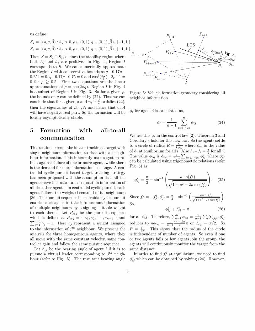
pursue a virtual leader corresponding to jth neigh-bour (refer to Fig. 5). The resultant bearing angle

P

Pi

Pi+1

P′

i+1

Pi+2

P′

i+2Pi+n−2

P′

i+n−2

Pi+n−1P

′

i+n−1

LOS

φi(n−1)φiφi2φi1

Vi

Figure 5: Vehicle formation geometry considering allneighbor information

φi for agent i is calculated as,

φi =1

n− 1

n∑

j=1, j 6=i

φij . (24)

We use this φi in the control law (2). Theorem 3 andCorollary 3 hold for this new law. So the agents settleto a circle of radius R = V

kφeqwhere φeq is the value

of φi at equilibrium for all i. Also hi−fi = π2 for all i.

The value φeq is φeq = 1n−1

∑n

j=1, j 6=i φ∗ij where φ∗ij

can be calculated using trigonometric relations (referFig. 5) as

φ∗ij =π

2− sin−1

ρ sin(f ji )

√

1 + ρ2 − 2ρ cos(f ji )

. (25)

Since f ji = −f i

j , φ∗ji =

π2 +sin−1

(

ρ sin(fj

i)√

1+ρ2−2ρ cos(fj

i)

)

.

So,φ∗ij + φ∗ji = π (26)

for all i, j. Therefore,∑n

i=1 φeq = 1n−1

∑

i

∑

j 6=i φ∗ij

reduces to nφeq = 1n−1

(n−1)n2 π or φeq = π/2. So

R = 2Vkπ

. This shows that the radius of the circleis independent of number of agents. So even if oneor two agents fails or few agents join the group, theagents will continuously monitor the target from thesame distance.In order to find f j

i at equilibrium, we need to findφ∗ij which can be obtained by solving (24). However,

9

for n > 3, we do not get a unique solution for φ∗ijsince the number of variables are more than numberof equations. Hence we restrict our analysis to n = 3agents. However, we demonstrate in simulation (Sec8) that the control law performs as desired for n > 3agents.

For three agents, solving (24), we get φ∗12 = φ∗23 =φ∗31. Then, using (25), we get sin2 f2

1 = sin2 f32 =

sin2 f13 and cos f2

1 = cos f32 = cos f1

3 . From the ge-ometry of the problem, f2

1 + f32 + f1

3 = 2πd withd = ±1,±2, . . .. Using all these conditions, we geteither f2

1 = f32 = f1

3 = 2πd/3 or two of the f i+1i

are equal to 2π and the other one is equal to −2π.Since the information of all the neighbours are con-sidered, strict indexing of the agents are not neces-sary. Therefore, we can relabel them once they arein the formation. Here, we label them sequentiallyby moving in anti-clockwise direction. This will gen-erate d = 1 formation only. Let us define §2 ={(2π, 2π,−2π), (2π,−2π, 2π), (−2π, 2π, 2π)}. Then,the states at equilibrium are given as

xi(1) =2V

kπ, xi(3) =

π

2, i = 1, 2, 3

(x1(2), x2(2), x3(2)) ∈{

§2,(

2π

3,2π

3,2π

3

)}

(27)

This implies that there are two equilibrium forma-tions possible - one where the vehicles are uniformlyplaced and the other where they are clustered to-gether as one unit as they move around the target. Inthe following theorem we show that the equilibriumformation with uniform distribution of the agents is alocally asymptotically stable formation whereas theformation with all the agents clustered together isunstable.

For a group of three agents with all-to-all com-munication, the uniform distribution of the agents asthey circle around the target is locally asymptoticallystable.

The equilibrium points are given in (27). We lin-earise the system (4) about the equilibrium points tostudy the local asymptotic stability.

Formation with cluster of agents

Linearising the system of three agents about equi-librium point described by R = 2V

kπ, (f2

1 , f32 , f

13 ) ∈ §2

and hi − fi = π2 , i = 1, 2, 3, we getX = AX where

A = circ (A1, A2, 03×3) with

A1 =

0 0 −VVR2 0 0VR2

−kρ1−ρ

0

A2 =

0 0 0−VR2 0 0

0 −kρ2(1−ρ) 0

Diagonalising A using Fourier matrix F3 we get Di =A1 + ςi−1A2, i ∈ {1, 2, 3}. The eigenvalues of A aresame as eigenvalues of Di, i = 1, · · ·n. So we cancomment about the stability of n vehicle system, byobserving the eigenvalues of each blockDi. The char-

acteristic equation of D1 block is s3+ks2+ V 2

R2 s. The

eigenvalues are at s = 0, s = −k2 ± k

2

√1− π2 which

are in left half of s-plane. The characteristic equation

corresponding to blockD2 is s3+ks2+ V 2

R2 s− 3V 2kρ2R2(1−ρ) .

As the last coefficient is negative using Routh - Hur-witz criterion we can conclude that the system is un-stable. Therefore a equilibrium with cluster of agentsis unstable.Formation with uniform distribution of agentsLinearising the system of three agents about equi-

librium point described by R = 2Vkπ

, f i+1i = 2π

3 and

hi − fi = π2 , i = 1, 2, 3, we get X = AX where

A = circ (A1, A2, A3) with

A1 =

0 0 −VVR2 0 0VR2

kρ(ρ+0.5)1+ρ+ρ2 −k

A3 =

0 0 00 0 0√3kρ

4R(1+ρ+ρ2) 0 0

A2 =

0 0 0−VR2 0 0

−√3kρ

4R(1+ρ+ρ2)kρ(ρ+0.5)2(1+ρ+ρ2) 0

The block circulant matrix A can be diagonalised us-ing Fourier matrix F3 as A = (F3 ⊗ I3)

?D(F3 ⊗ I3)where (?) indicates conjugate transpose. The diag-onal matrix D is given by D = diag (D1, D2, D3)where Di = A1 + ςi−1A2 + ς2(i−1)A3, i ∈ {1, 2, 3}.The eigenvalues of A are same as eigenvalues ofDi, i = 1, · · ·n. Substituting the value of R, eachDi can be factorised as Di = kT−1DiT , whereT =diag[k, V, V ] and

Di =

0 0 −1π2

4 (1 − ςi−1) 0 0π2

4 +√3ρπ(ς2(i−1)−ςi−1)

8(1+ρ+ρ2)ρ(ρ+0.5)1+ρ+ρ2 (1 +

ςi−1

2 ) −1

.

10

0 0.1 0.2 0.3 0.4 0.5 0.6 0.7 0.8 0.9 10

2

4

6

8

10

12

14

16

18

ρ −−−>

h1h2h3

Figure 6: Variation of h1, h2 and h3 versus ρ underall-to-all communication

The spectrum σ(·) of Di and Di are related asσ(Di) = kσ(Di). Since k > 0 , stability of Di canbe determined from the stability of Di. As Di doesnot have a term containing gain k as well as V , wecan conclude that the stability of this formation isindependent of k and V .

The characteristic equation ofD1 block is s3+ks2+

V 2

R2 s. So the eigenvalues are at s = 0, s = −k2 ±

k2

√1− π2 which are in left half of s-plane. For i =

2, 3, Di is a complex matrix, as ςi−1 = e2πji−1n is a

complex quantity. The characteristic polynomial ofDi can be written as PDi

(λ) = λ3 + c1λ2 + c2λ+ c3,

where c1 = 1, c2 = 3π2ρ(ρ+0.5)8(1+ρ+ρ2) and c3 = a3 + jb3

wherea3 = π2

4 +√3ρπ

8(1+ρ+ρ2) (cos(4π(i−1)

3 )− cos(2π(i−1)3 )) ,

b3 =√3ρπ

8(1+ρ+ρ2) (sin(4π(i−1)

3 )− sin(2π(i−1)3 )).

Let H be the Hermitian matrix corresponding tothe characteristic polynomial PDi

(λ). Then the poly-nomial PDi

(λ) is asymptotically stable if and only ifthe principal minors h1, h2 and h3 of H are posi-tive [35]. In this case h1 = 2, h2 = 4(a2 − a3) and8(a2

2a3−2a2a32− b32+a33). Here h1, h2 and h3 are

functions of only ρ. Fig. 6 shows the variation of h1,h2 and h3 for ρ ∈ (0, 1). For all ρ, these values arepositive which implies that the system is stable forall values of ρ. Therefore, for three agents we willget uniform formation around the target.

6 Implementation with 6-DOFModel

In this section, we discuss implementation of theproposed strategy for fixed-wing MAVs. The flightmodel is taken from [37], in which the wind tunneldata was obtained from National Aerospace Labora-tories, Bangalore. The aerodynamic equations usedare as follows:

xe = [u cos θ + (v sinφ+ w cosφ) sin θ] cosψ

− (v cosφ− w sinφ) sinψ

ye = [u cos θ + (v sinφ+ w cosφ) sin θ] sinψ

+ (v cosφ− w sinφ) cosψ

ze = −u sin θ + (v sinφ+ w cosφ) cos θ

θ = q cosφ− r sinφ

φ = p+ (q sinφ+ r cosφ) tan θ

ψ =(q sinφ+ r cosφ)

cos θ

u = rv − qw +1

mfx

v = pw − ru+1

mfy

w = qu− pv +1

mfz

p = Γ1pq − Γ2qr + Γ3l + Γ4n

q = Γ5pr − Γ4

(

p2 − r2)

+ Γ5m

r = Γ6pq − Γ1qr + Γ4l + Γ7n

where [xe, ye, ze] represent position of MAV, [u, v, w]represent velocity components of MAV in bodyframe, [φ, θ, ψ] represent Euler angles, [p, q, r] rep-resent body axis angular rates and [l,m, n] are roll,pitch and yaw moments. During the flight the alti-tude and airspeed are held constant. Autopilot ofeach MAV has three controllers to regulate head-ing, speed and altitude using proportional-integral-derivative (PID) control loops. The autopilot designis the same as give in [37]. There are two separateautopilots for the longitudinal and lateral control.The motivation for this comes from the fact that,upon linearization of the flight mechanics relationsgiven above about trim conditions for steady level

11

flight, the longitudinal and lateral dynamics get de-coupled. The longitudinal and lateral autopilots aredesigned using successive loop closure [38]. Thereare two inputs to the longitudinal autopilot - com-manded airspeed (Vc) and commanded altitude (hc).Commanded speed (Vc) is held constant. Also thecommanded altitude (hc) is held constant for sim-ulating planar condition. Speed control is achievedby controlling throttle input. To avoid possibilityof collisions each MAV is commanded to fly at dif-ferent altitudes. The altitude control loop generatesappropriate commands for elevator defection of theMAV. Lateral autopilot command is generated us-ing desired heading angle. The desired heading angleor heading command χic is calculated using desiredbearing angle as discussed in Section 4 (Equation 2).From flight mechanics, the heading rate of MAV canbe calculated as:

χi = −p sin θ + q cos θ sinφ+ r cosφ sin θ.

The Runge-Kutta fourth order method has been usedto solve the system of equations with the time stepof dT = 2 msec. It is assumed that the position in-formation is available at discrete instances (one secin accordance to the GPS module) and the autopi-lot controllers run at a frequency of 20 msec. Theheading command of MAV is updated at every onesec using the position information of the next MAVto be followed and the MAV’s own position update(The frequencies of both GPS updates of inter-MAVcommunication are taken to be 1 Hz to mimic thethe timings implemented on the HILS). The head-ing error χie between the heading command χic andheading angle χi is computed as χie = χic − χi andthe roll angle command φic for the inner loop rollcontroller is generated as:

φic = HKpχie −HKdχi

where HKp is proportional gain and HKd is deriva-tive gain. Here HKp is related to controller gain k(Equation (2)) as HKp = Vik/g where Vi is the speedof the vehicle i and g is acceleration due to gravity.The roll command is tracked by the inner PID controlloop and it generates appropriate actuation commandfor aileron defection. The same autopilot controllers

and timing intervals have been implemented on HILSwhich is discussed in following section.

7 Hardware in Loop Simula-tor(HILS)

The HILS system can broadly be classified into twoparts, as shown in figure 7 – the simulated compo-nents and the actual hardware subsystems presentin the simulation loop. Flight dynamics and sensordynamics have been simulated as SimuLink Blocksin MATLAB on the host PC. This SimuLink modelis compiled in C programs when it is built for thexPC TargetTMRapid Prototyping System v5.0 and isloaded onto the Target PC to be run in real time.The flight simulation generates the sensor data forthe On Board Computers (OBCs) in appropriate for-mats. The sensor information includes the GPS andIMU sentences as well as analog voltages for altitudeand airspeed measurements. These sentences are seri-ally conveyed via a serial card on the Target PC to theOBCs at correct baud-rates after regular intervals.The pressure sensor data for airspeed and altitude isconverted to analog voltages with proper scaling andsent to OBCs on-board ADC. The control algorithmresides on the OBCs which gives commands to servo-motors used for surface deflection. Analog feedbackfrom the servomotors is given as input to the flightsimulation. The XBee - Pro RF module has beenused for communication between the MAVs and alsowith the ground station. All the communication linksutilize the API (Application Programming Interface)mode of addressed packet based communication al-lowing both one to one and broadcast communica-tion. The ground station has been used for monitor-ing the MAV flight parameters and for tuning gainsof autopilots programmed on the OBC during thereal-time HILS simulations.

12

Figure 7: Block diagram of the HILS system for for real time simulation of cooperative missions of eightMAVs.

Table 1: Comparison between Analytical and Simu-lation results with cyclic communication

r RCases Analytical Simulation Analytical Simulation8.1 13.504 13.504 6.926 6.9268.1 12.745 12.745 8.150 8.1508.1 11.485 11.485 5.890 5.8908.1 15.859 15.859 10.142 10.142

8 Simulation Results

8.1 Stability with unicycle agents incyclic communication

We considered seven agents with cyclic communica-tion all moving with unit speed and having controllergain k = 0.1. The target is stationary and is locatedat the origin (0,0). ρ and initial d have been selectedsuch that the agents are initially at equilibrium andthe equilibrium points lie in one of the sector I, II,III and IV of Fig. 4.

Assume the agents are initially in the {7/3} forma-tion with ρ = 0.4. Here R = 6.9256 initially and thisformation corresponds to Section I in Fig. 4. FromTable 2 , it is clear that both h2 and h3 are posi-tive. So, this is a case of stable formation. Theorem3 is also satisfied since, ql = 0.186 , qu = 0.818 anddn

= 0.4286. Fig. 8(a) shows that, at equilibriumit stays in {7/3} formation and the analytical val-ues of r and R match with the values obtained fromsimulation as shown in Table 1.

In this case, the agents are initially in {7/1} for-mation, distributed along a circle of radius R = 8.503with target at the center. The value of ρ = 0.4. From(23), the limits for d

nare ql = 0.188 and qu = 0.818.

As dn

= 1/7 = 0.143, it corresponds to a point inSection II of Fig. 4. Therefore this violates Theo-rem 3. It is also evident from the Table 2 that thevalue of h3 < 0 for all Di, for i = 2, ..., 7. There-fore, this is a case of unstable formation. Fig. 8(b)shows that, even though the agents are initially in{7/1} formation, the system finally settles down tothe {7/2} formation. As shown in Table 1, analyti-cal and simulated values of r and R are the same atequilibrium. The {7/2} formation for ρ = 0.4 corre-sponds to Section I of Fig. 4.

13

Table 2: h2 and h3 values for all Di blocks with cyclic communicationCase 1 Case 2 Case 3 Case 4

d = 3, ρ = 0.4 d = 1, ρ = 0.4 d = 6, ρ = 0.4 d = 4, ρ = 0.8Block h2 h3 h2 h3 h2 h3 h2 h3D1 8.34 0 5.53 0 15.45 0 12.53 0

D2 7.63 5.28 5.89 -2.38 12.73 -11.58 10.15 15.16

D3 6.10 10.75 7.99 -10.70 10.18 -34.38 4.64 8.04

D4 4.95 12.84 10.95 -22.42 11.70 -69.91 0.47 -0.86

D5 4.95 12.84 10.95 -22.42 11.70 -69.91 0.47 -0.86

D6 6.10 10.75 7.99 -10.70 10.17 -334.38 4.64 8.04

D7 7.63 5.28 5.89 -2.38 12.73 -11.58 10.05 15.16

Similar to the previous case, agents are initiallyin the {7/6} formation with ρ = 0.4. So initiallyR = 5.0875 and corresponds to a point in SectionIII of Fig. 4. Table 2 shows that the value of h3 isnegative in this case. As d

n= 6/7 = 0.8571, which is

outside the stable range ql = 0.186 and qu = 0.818,it is an unstable case according to Theorem 3. Fig.8(c) confirms this result and shows that the systemeventually converges to the {7/4} formation. Table1 shows that the analytical and simulation resultscorresponding to final formation matches.

In this case, agents are initially in the {7/4} for-mation with ρ = 0.8. R = 5.6502 and d

n= 0.5714.

This corresponds to a point in Section IV of Fig. 4.From Table 2 , h3 < 0 for some of the Di blocks. Alsoas d

n> qu = 0.4359, d

ndoes not satisfy the bounds

in (22). The simulation result shown in Fig. 8(d)proves the instability of the formation. The agentssettle with the {7/2} formation at equilibrium andthe values of r and R are same both in simulationand in theory (refer to Table 1.

8.2 Comparison of performance usingunicycle, 6DOF model and HILS

(With cyclic communication): A set of three vehiclesmoving with a constant speed of 15 m/sec and con-troller gain of 0.2 have been considered. The vehiclesstart from random initial positions. Figure 9 showsthe trajectories of the vehicles with unicycle model,

Table 3: Steady state parameters in cyclic communi-cation for different values of pursuit gain ρ

Unicycle 6-DOF HILSρ d Radius Radius Error (%) Radius Error(%)0.1 2 66.6235 69.4026 4.17 64.1837 3.660.2 1 77.8567 79.854 2.56 76.4984 1.740.3 1 81.6677 84.0749 2.94 81.5176 0.830.4 1 85.3938 88.189 3.27 86.3877 1.160.5 2 57.8372 57.6884 0.26 56.8479 1.710.6 2 56.4505 56.1376 0.55 55.2274 2.160.7 2 55.2661 54.8134 0.82 54.5251 1.340.8 2 54.246 53.8636 0.70 54.2912 0.080.9 2 53.3608 54.2482 1.66 55.0426 3.15

6 - DOF model and HILS with ρ = 0.5 and with thesame initial positions of the vehicles. The vehicles areable to capture the target and are uniformly distribu-tion. The evolution of the trajectory of the vehiclesvaries with the model of the vehicle as seen in thefigures. However, the final formation around the tar-get remains the same. Table 3 shows the radius ofthe circle at steady state for different values of ρ. Itcan be seen that the error in the radius is with 5% ofthe analytical value. Thus, the analytical results canbe used for target tracking applications using microaerial vehicles.(With all-to-all communication): We simulated forfour vehicles. The vehicles move with a constantspeed of 15 m/sec and controller gain of 0.2, starting

14

−10 −8 −6 −4 −2 0 2 4 6 8 10−8

−6

−4

−2

0

2

4

6

8

1

2

3

4

5

6

7

Target

X−axis

Y−

axis

(a) {7/3} → {7/3}

−10 −5 0 5 10−10

−8

−6

−4

−2

0

2

4

6

8

10

1

2

3

4

5

6

7

Target

X−axis

Y−

axis

(b) {7/1} → {7/2}

−8 −6 −4 −2 0 2 4 6 8

−6

−4

−2

0

2

4

6

1

2

3

4

5

6

7

Target

X−axis

Y−

axis

(c) {7/6} → {7/4}

−25 −20 −15 −10 −5 0 5 10 15 20 25

−20

−15

−10

−5

0

5

10

15

20

1

2

3

4

5

6

7

Target

X−axis

Y−

axis

(d) {7/4} → {7/2}

Figure 8: Stable and unstable formation of seven ho-mogeneous agents in cyclic communication.

(a) Unicycle model

(b) 6-DOF MAV model

(c) HILS simulation

Figure 9: Trajectories of the agents in cyclic commu-nication with ρ = 0.5

15

−500 −400 −300 −200 −100 0 100 200 300−500

−400

−300

−200

−100

0

100

200

X (m)−−−>

Y (

m)−

−−

>

Agent01Agent02Agent03Agent04Target

(a) Unicycle model

−500 −400 −300 −200 −100 0 100 200 300

−500

−400

−300

−200

−100

0

100

X(m) −−−>

Y(m

)−−

−>

Agent1Agent2Agent3Agent4

(b) 6-DOF MAV model

−600 −500 −400 −300 −200 −100 0 100 200

−500

−400

−300

−200

−100

0

100

X (m) −−−−>

Y (

m)

−−

−−

>

Agent1Agent2Agent3Agent4

(c) HILS simulation

Figure 10: Trajectories of the agents with all-to-allcommunication

from random initial positions. Simulations are runfor different values of ρ. Figure 10 shows the tra-jectories of the vehicles with point mass model, 6 -DOF model and HILS for ρ = 0.5 and for the sameinitial conditions. The vehicles are able to capturethe target with uniform distribution. Table 4 showsdifferent parameters at steady state for different val-ues of ρ. This shows that the uniform formation isstable in case of all-to-all communication even whenn > 3.

Table 4: Steady state parameters with all-to-all com-munication and different values of pursuit gain ρ

Point mass 6-DOF HILSρ Radius Radius Error(%) Radius Error(%)0.1 70.11 73.36 4.63 66.33 5.390.2 70.11 73.37 4.64 65.71 6.280.3 70.11 73.39 4.67 66.65 4.940.4 70.11 73.41 4.70 67.29 4.010.5 70.11 73.43 4.72 70.01 0.130.6 70.11 73.46 4.77 68.347 2.530.7 70.11 73.55 4.90 69.48 0.900.8 70.11 73.57 4.92 68.85 1.800.9 70.11 73.6 4.96 70.90 1.11

8.3 Moving target case with cycliccommunication

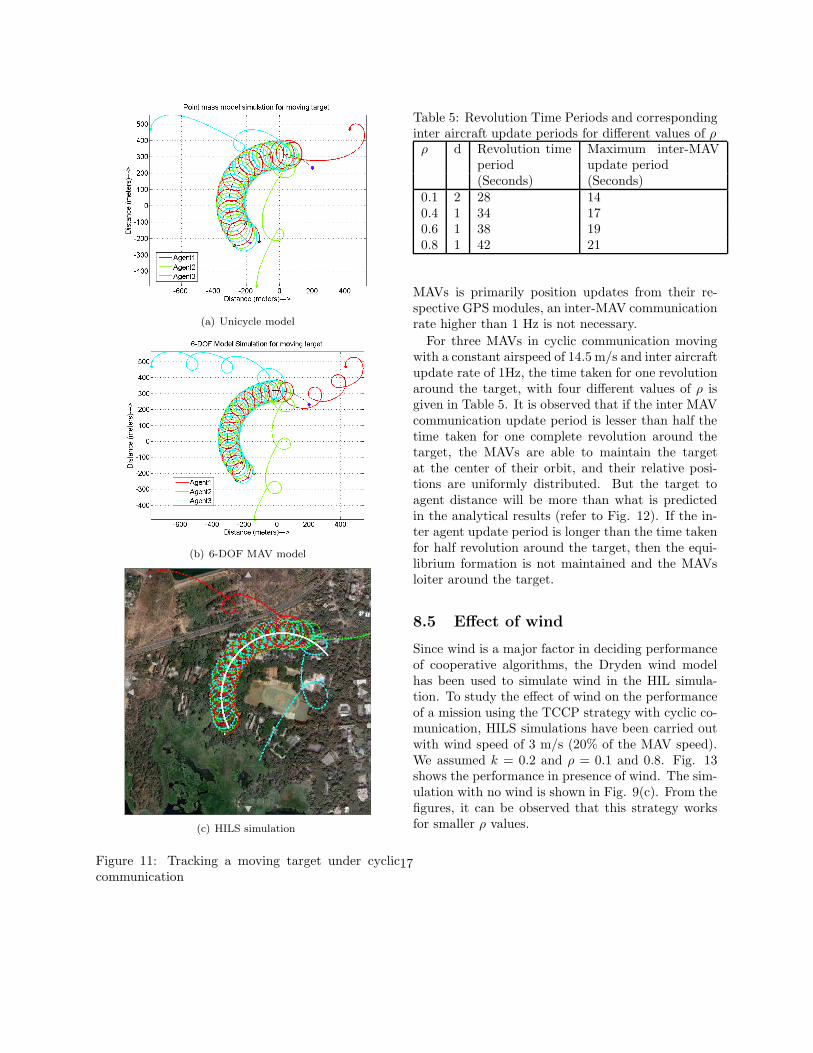
We present a typical case here. The target is assumedto move with a velocity of 2 m/s along a circle of ra-dius 300 meters. The three MAVs have been placedrandomly and are moving with a speed of 15m/s.The controller gain is 0.2 and ρ = 0.2 and the ve-hicles are cyclic communication. The trajectory ofthe vehicle when modelled as unicycle is shown inFig. 11(a). When the vehicles have 6DOF dynamicalmodel, their trajectory is shown in Fig. 11(b). Thetrajectory obtained in HILS is shown in Fig. 11(c).From the figure we can conclude the TCCP can tracka slowly moving target.

8.4 Effect of inter-MAV update fre-quency

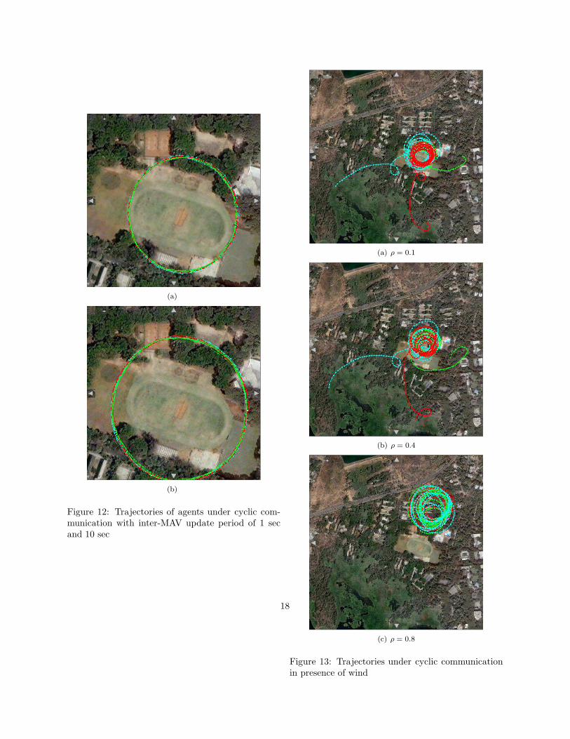
In a realistic settings, there could be intermit-tent communication failures which would cause lossof communication packets among the cooperatingagents. Since this cannot be avoided, it is beneficialto have a cooperative strategy that would be ableto tolerate such practical constraints. With this inmind, the simulation results presented in this sectiongive an idea about the smallest inter aircraft updaterate that our strategy can tolerate. The GPS mod-ule simulated in the HILS has a position update rateof 1Hz. Since the information communicated among

16

(a) Unicycle model

(b) 6-DOF MAV model

(c) HILS simulation

Figure 11: Tracking a moving target under cycliccommunication

Table 5: Revolution Time Periods and correspondinginter aircraft update periods for different values of ρρ d Revolution time

periodMaximum inter-MAVupdate period

(Seconds) (Seconds)0.1 2 28 140.4 1 34 170.6 1 38 190.8 1 42 21

MAVs is primarily position updates from their re-spective GPS modules, an inter-MAV communicationrate higher than 1 Hz is not necessary.

For three MAVs in cyclic communication movingwith a constant airspeed of 14.5 m/s and inter aircraftupdate rate of 1Hz, the time taken for one revolutionaround the target, with four different values of ρ isgiven in Table 5. It is observed that if the inter MAVcommunication update period is lesser than half thetime taken for one complete revolution around thetarget, the MAVs are able to maintain the targetat the center of their orbit, and their relative posi-tions are uniformly distributed. But the target toagent distance will be more than what is predictedin the analytical results (refer to Fig. 12). If the in-ter agent update period is longer than the time takenfor half revolution around the target, then the equi-librium formation is not maintained and the MAVsloiter around the target.

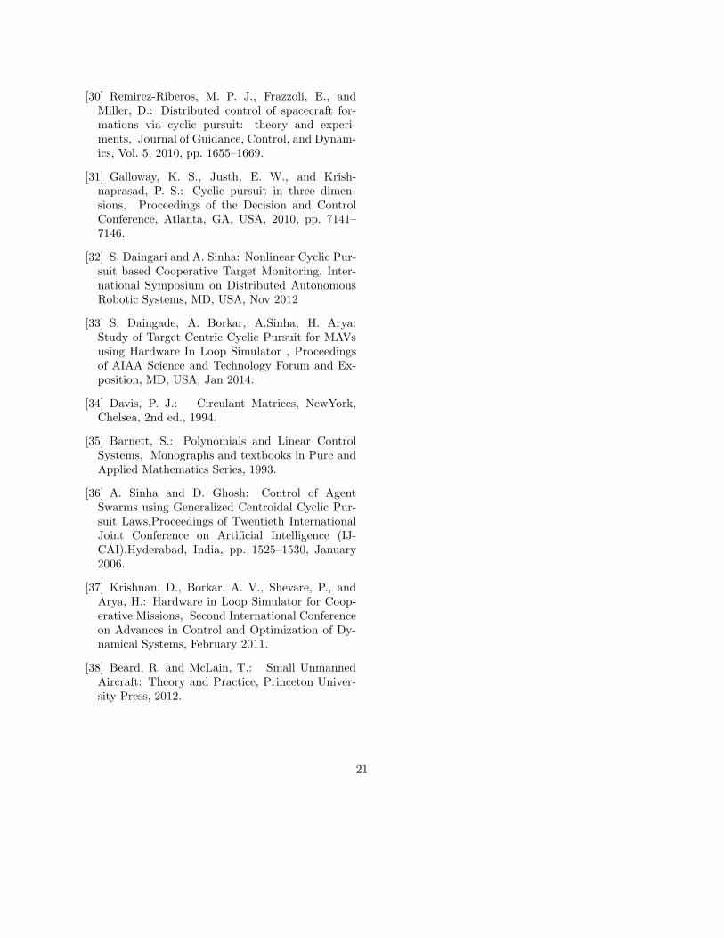
8.5 Effect of wind

Since wind is a major factor in deciding performanceof cooperative algorithms, the Dryden wind modelhas been used to simulate wind in the HIL simula-tion. To study the effect of wind on the performanceof a mission using the TCCP strategy with cyclic co-munication, HILS simulations have been carried outwith wind speed of 3 m/s (20% of the MAV speed).We assumed k = 0.2 and ρ = 0.1 and 0.8. Fig. 13shows the performance in presence of wind. The sim-ulation with no wind is shown in Fig. 9(c). From thefigures, it can be observed that this strategy worksfor smaller ρ values.

17

(a)

(b)

Figure 12: Trajectories of agents under cyclic com-munication with inter-MAV update period of 1 secand 10 sec

(a) ρ = 0.1

(b) ρ = 0.4

(c) ρ = 0.8

Figure 13: Trajectories under cyclic communicationin presence of wind

18

9 Conclusion

This paper proposes a new strategy called the targetcentric cyclic pursuit. This is a variant of the cyclicpursuit strategy that can be used for target track-ing applications. Mathematical formulation and theanalysis have been carried out for this strategy usingunicycle models of the agents and a stationary tar-get. Two types of information exchange among theagents have been considered - cyclic and all-to-all.It is found that at equilibrium, the agents move ina polygonal formation around the target with equalangular speeds. The necessary conditions for the exis-tence of the equilibrium have been derived. The localstability analysis of the equilibrium formations haveshown that the pursuit gain ρ plays an important rolein the formation that is achieved at equilibrium.

The proposed strategy is then applied to the 6DOFmodel of the micro aerial vehicles. The simulationresults closely matched with the analysis done usingunicycle model. As the next step, the strategy istested on Hardware-in-Loop Simulator and the per-formance was satisfactory. The error in the analyticalresults and in HILS was less then 5%. The strategyeven works for a slowly moving target. This givesthe confidence that the proposed strategy will per-form as desired when it is applied on actual hard-ware. We also tested different cases that are likelyto occur in such missions, for example, the effect ofwind disturbance and the effect of changing the fre-quency of updates from the neighbours. The futurework would be to extend this strategy for multiplemoving targets.

References

[1] Cao, Y., Yu, W., Ren, W., Chen G.: An Overviewof Recent Progress in the Study of DistributedMulti-agent Coordination, IEEE Transactions onIndustrial Informatics, Vol. 09(01), 2013, pp. 427–438.

[2] Kobayashi, K., Otsubo, K., and Hosoe, S.: De-sign of decentralized capturing behavior by mul-tiple robots, IEEE Workshop on Distributed In-

telligent Systems: Collective intelligence and itsApplications, June 2006, pp. 463–468.

[3] Guo, J., Yan, G., and Lin, Z.: Local control strat-egy for moving-target-enclosing under dynamicallychanging network topology, Systems & ControlLetters, Vol. 59 (10), 2010, pp. 654–661.

[4] Kim, Y. and Sugie, T.: Cooperative control fortarget-capturing task based on a cyclic pursuitstrategy, Automatica, Vol. 43(08), 2007, pp. 1426–1431.

[5] Ma, L. and Hovakimyan, N.: Vision-Based CyclicPursuit for Cooperative Target Tracking, Pro-ceedings of the American Control Conference, June2011, pp. 4616–4621.

[6] Paley, D., Leonard, N., and Sepulchre, R.: Col-lective motion: bistability and trajectory tracking,Proceedings of the 43rd IEEE Conference on Deci-sion and Control, December 2004, pp. 1932–1937.

[7] Napora, S. and Paley, D.: Observer - Based feed-back control for stabilization of collective motion,IEEE Transactions on Control Systems Technol-ogy, Vol. 21(05), 2013, pp. 1846–1857.

[8] Klein, D. J. and Morgansen, K. A.: Controlledcollective motion for mulitvehicle trajectory track-ing, Proceedings of the American Control Confer-ence, June 2006, pp. 5269–5275.

[9] Klein, D. J., Matlack, C., and Morgansen, K. A.:Cooperative target tracking using oscillator modelsin three dimensions, Proceedings of the AmericanControl Conference, July 2007, pp. 2569–2575.

[10] Ceccarelli, N., Marco, M. D., Garulli, A., andGiannitrapani, A.: Collective circular motion ofmulti-vehicle systems, Automatica, Vol. 44(12),2008, pp. 3025–3035.

[11] Kingston, D. and Beard, R.: UAV Splay stateconfiguration for moving targets in wind, Ad-vances in coperative control and optimization, Lec-ture notes in Computer Science, 2008, pp. 109–128.

19

[12] Yongcan Cao; Muse, J.; Casbeer, D.; Kingston,D., : Circumnavigation of an unknown target us-ing UAVs with range and range rate measurementsProceedings of the IEEE Conference on Decisionand Control, Dec. 2013, pp. 3617–3622,

[13] Lan, Y., Yan, G., and Lin, Z.: A hybrid controlapproach to coperative target tracking with mul-tiple mobile robots, Proceedings of the AmericanControl Conference, June 2009, pp. 2624–2629.

[14] Lan, Y., Yan, G., and Lin, Z.: Distributed con-trol of cooperative target enclosing based on reach-ability and invariance analysis, Systems & ControlLetters, Vol. 59(07), 2010, pp. 381–389.

[15] Mangal Kothari, Rajnikant Sharma, IanPostlethwaite, Randal W. Beard, Daniel Pack:Cooperative target capturing with incompletetarget information, Journal of Intelligent andRobotic Systems, Volume 72, Issue 3-4, pp.373-384, December 2013,

[16] Chen, Z. and Zhang, H.: No-beacon collectivecircular motion of jointly connected multi-agents,Automatica, Vol. 47), 2011, pp. 1929–1937.

[17] Moshtagh, N., Michael, N., Jadbabaie, A., andDaniilidis, K.: Vision-Based, Distributed Con-trol Laws for Motion Coordination of Nonholo-nomic Robots, IEEE Transactions on Robotics,Vol. 25(04), August 2009, pp. 851–860.

[18] Ma, L. and Hovakimyan, N.: Cooperative TargetTracking in Balanced Circular Formation: Multi-ple UAVs Tracking a Ground Vehicle, Proceedingsof the American Control Conference, June 2013,pp. 5386–5391.

[19] Bakolas, E. and Tsiotras, P.: On the Relay Pur-suit of maneuvering target by a group of pursuers,Proceedings of the IEEE conference on Decisionand Control and European Control Conference,December 2011, pp. 4270–4275.

[20] Olfati-Sabar, R. and Sandell, N. F.: Distributedtracking in sensor networks with limited sensingrange, Proceedings of the American Control Con-ference, June 2008, pp. 3157–3162.

[21] Petitti, A., Paola, D., Rizzo, A., and Cicirelli,G.: Consensus-based distributed estimation fortarget tracking in heterogeneous networks, Pro-ceedings of the IEEE conference on Decision andControl and European Control Conference, De-cember 2011, pp. 6648–6653.

[22] Bruckstein, A., Cohen, N., and Efrat, A.: Ants,Crickets and frogs in cyclic pursuit, Centerfor Intelligence Systems,Technical Report 9105,Technion-Israel Institute of Technology, Haifa, Is-rael, 1991.

[23] Bruckstein, A.: Why the ant trail look sostraight and nice, The Mathematical Intelligencer,Vol. 15(02), 1993, pp. 59–62.

[24] Sinha, A. and Ghosh, D.: Generalization of lin-ear cyclic pursuit with application to rendezvous ofmultiple autonomous agents, IEEE Transactionson Automatic Control, Vol. 51(11), 2006, pp. 1818–1824.

[25] Marshall, J. A., Broucke, M. E., and Fran-cis, B. A.: Formations of Vehicles in Cyclic Pur-suit, IEEE Transaction on Automatic Control,Vol. 49(11), 2004, pp. 1963–1974.

[26] Sinha, A. and Ghosh, D.: Generalization of Non-linear Cyclic pursuit, Automatica, Vol. 43(11),2007, pp. 1954–1960.

[27] Rattan, G. and Ghosh, D.: Nonlinear cyclic pur-suit strategies for MAV swarms, Technical Report,DRDO-IISc Programme on Advanced Research inMathematical Engineering, 2009, pp. 1–32.

[28] Pavone, M. and Frazzoli, E.: Decentralized poli-cies for geometric pattern formation and pathcoverage, ASME Journal on Dynamic Systems,Measurement, and Control, Vol. 129(05), 2007,pp. 633–643.

[29] Ramirez, J.: New decentralized algorithms forspacecraft formation control based on a cyclic ap-proach, Ph.D. dissertation, Massachusetts Insti-tute of Technology, Boston, 2010.

20

[30] Remirez-Riberos, M. P. J., Frazzoli, E., andMiller, D.: Distributed control of spacecraft for-mations via cyclic pursuit: theory and experi-ments, Journal of Guidance, Control, and Dynam-ics, Vol. 5, 2010, pp. 1655–1669.

[31] Galloway, K. S., Justh, E. W., and Krish-naprasad, P. S.: Cyclic pursuit in three dimen-sions, Proceedings of the Decision and ControlConference, Atlanta, GA, USA, 2010, pp. 7141–7146.

[32] S. Daingari and A. Sinha: Nonlinear Cyclic Pur-suit based Cooperative Target Monitoring, Inter-national Symposium on Distributed AutonomousRobotic Systems, MD, USA, Nov 2012

[33] S. Daingade, A. Borkar, A.Sinha, H. Arya:Study of Target Centric Cyclic Pursuit for MAVsusing Hardware In Loop Simulator , Proceedingsof AIAA Science and Technology Forum and Ex-position, MD, USA, Jan 2014.

[34] Davis, P. J.: Circulant Matrices, NewYork,Chelsea, 2nd ed., 1994.

[35] Barnett, S.: Polynomials and Linear ControlSystems, Monographs and textbooks in Pure andApplied Mathematics Series, 1993.

[36] A. Sinha and D. Ghosh: Control of AgentSwarms using Generalized Centroidal Cyclic Pur-suit Laws,Proceedings of Twentieth InternationalJoint Conference on Artificial Intelligence (IJ-CAI),Hyderabad, India, pp. 1525–1530, January2006.

[37] Krishnan, D., Borkar, A. V., Shevare, P., andArya, H.: Hardware in Loop Simulator for Coop-erative Missions, Second International Conferenceon Advances in Control and Optimization of Dy-namical Systems, February 2011.

[38] Beard, R. and McLain, T.: Small UnmannedAircraft: Theory and Practice, Princeton Univer-sity Press, 2012.

21