feasibility of applying controllable lubrication
TRANSCRIPT

General rights Copyright and moral rights for the publications made accessible in the public portal are retained by the authors and/or other copyright owners and it is a condition of accessing publications that users recognise and abide by the legal requirements associated with these rights.
• Users may download and print one copy of any publication from the public portal for the purpose of private study or research. • You may not further distribute the material or use it for any profit-making activity or commercial gain • You may freely distribute the URL identifying the publication in the public portal
If you believe that this document breaches copyright please contact us providing details, and we will remove access to the work immediately and investigate your claim.
Downloaded from orbit.dtu.dk on: Dec 17, 2017
Feasibility of Applying Controllable Lubrication Techniques to Reciprocating Machines
Pulido, Edgar Estupinan; Santos, Ilmar
Publication date:2009
Document VersionPublisher's PDF, also known as Version of record
Link back to DTU Orbit
Citation (APA):Pulido, E. E., & Santos, I. (2009). Feasibility of Applying Controllable Lubrication Techniques to ReciprocatingMachines. Kgs. Lyngby, Denmark: Technical University of Denmark (DTU). (DCAMM Special Repport; No.S111).

Feasibility of Applying Controllable Lubrication Techniques to Reciprocating Machines
Ph
D T
he
sis
Edgar Estupiñan PulidoDCAMM Special Repport No. S111December 2009


Feasibility of Applying Controllable Lubrication Techniquesto Reciprocating Machines
Edgar Estupinan Pulido
Department of Mechanical EngineeringTechnical University of Denmark

Title of the thesis:Feasibility of Applying Controllable Lubrication Techniquesto Reciprocating Machines
Ph.D. student:Edgar Estupinan PulidoE-mail: [email protected]
Supervisor:Ilmar Ferreira SantosE-mail: [email protected]
Address:Nils Koppels Alle, Building 404, DK-2800.Kgs. Lyngby, DenmarkDepartment of Mechanical EngineeringTechnical University of Denmark
Copyright © 2010 Edgar Estupinan Pulido
ISBN 978-87-89502-95-3
Preface
This thesis is submitted as partial fulfilment of the requirements for awarding the Danish Ph.D. de-gree. The work was carried out from September 2006 to December 2009 at the Department of Me-chanical Engineering (MEK ), Solid Mechanics (FAM ), Technical University of Denmark (DTU ).The project was supervised by Associate Professor Dr.-Ing. Ilmar Ferreira Santos.
First of all, I would like to thank my supervisor for his permanent support and guidance, and forinspiring me not only technically, but in many other aspects. I want to thank my closest colleaguesfrom DTU, Stefano Morosi, Martin Haugaard, Said Lahiri and the newcomer Alejandro Cerda, forthe pleasure of working together, for all the stimulating talks, and pleasure moments during theseyears. I also want to thank my former colleagues from DTU, Klaus Kjølhede and Niels Heinrichson,and to Professor Peder Klit, for making me feel welcome when I just arrived, and for introducingme to the Danish culture.
I specially want to thank my dear wife Yury, for making my life more enjoyable during all theseyears together, for her permanent support and encouragement, and for always being on my side.
I want to gratefully acknowledge the support given by the Programme Alβan, the European UnionProgramme of High Level Scholarships for Latin America, scholarship No. E06D101992CO. Lastbut not least, I wish to thank the support given by the University of Tarapaca, Chile.
I dedicate this work to my mother for making me always feel that geographical distances does notcount in a mother’s love, and to my son Simon for bringing so much joy to my life.
Technical University of DenmarkKgs. Lyngby, December 2009
Edgar Estupinan
iii

iv
Abstract
The use of active lubrication in journal bearings helps to enhance the thin fluid films by increasingthe fluid film thickness and consequently reducing viscous friction losses and vibrations. One refersto active lubrication when conventional hydrodynamic lubrication is combined with dynamicallymodified hydrostatic lubrication. In this case, the hydrostatic lubrication is modified by injecting oilat controllable pressures, through orifices circumferentially located around the bearing surface.
In order to study the performance of journal bearings of reciprocating machines, operating underconventional lubrication conditions, a mathematical model of a reciprocating mechanism connectedto a rigid / flexible rotor via thin fluid films was developed. The mathematical model involves theuse of multibody dynamics theory for the modelling of the reciprocating mechanism (rigid bodies),finite elements method for the modelling of the flexible rotor (crankshaft) and hydrodynamic fluidfilm theory for describing the dynamics of the thin fluid films. When active lubrication is intro-duced to modify conventional hydrodynamic lubrication, by means of aplying radial oil injectionat controllable oil pressures, the Reynolds equation is modified to accomodate the terms related tothe controllable oil injection pressures and orifice distribution on the bearing surface. The activebearing forces and the dynamics of the oil injection system are coupled to the set of nonlinear equa-tions that describes the dynamics of the reciprocating engine, obtained with the help of multibodydynamics (rigid components) and finite elements method (flexible components), and the global sys-tem of equations is numerically solved. The analysis of the results was carried out with focus onthe behaviour of the journal orbits, maximum fluid film pressure minimum fluid film thickness. Thereduction in the cyclic averaged power consumption due to viscous friction forces is also studied.
The modelling of two oil injection systems is presented in the work. The main governing equa-tions of the dynamics of a piezo-actuated oil injection system and a mechanical-actuated unit in-jector are developed. It is shown how the dynamics of the oil injection system is coupled to thedynamics of the bearing fluid film through equations. Applying controllable radial oil injection todynamically loaded journal bearings helps: a) to reduce friction losses by increasing the fluid filmthickness; b) to reduce vibrations (i.e., smaller journal centre orbits); and c) to increase the effectivecarrying load area by modifying the pressure distribution profile, which can make it possible to usebearings of smaller dimensions with similar load-carrying capacity.
v

vi
Resume (in Danish)
Anvendligheden af aktiv smøring i reciprokerende maskiner
Brugen af aktiv smøring i glidelejer forøger tykkelsen af smørefilmen, hvorved tab fra viskos frik-tion og vibrationer mindskes. Konventionel hydrodynamisk smøring kombineret med dynamiskmodificeret hydrostatisk smøring, kaldes aktiv smøring. Her modificeres den hydrostatiske smøringved at injicere olie igennem dyser i lejets overflade.
For at studere egenskaberne af glidelejer i stempel maskiner under konventionelle smøringsbetin-gelser er en matematisk model af en krumtapmekanisme forbundet til en stiv / fleksibel rotor via envæskefilm udarbejdet. Den matematiske model involverer brugen af “multi-body-dynamic” teori tilmodelleringen af en krunmtapmekanisme, “Finite Element” metoden bruges til modellering af denfleksible rotor (krumtappen) og hydrodynamisk smørefilmteori bruges til at beskrive dynamikkenaf væskefilmen. Nar aktiv smøring introduceres for at modificere den konventionelle hydrody-namiske smøring, ved hjælp af radial indsprøjtning af olie, modificeres Reynolds ligning med ledder beskriver indsprøjtningen. De aktive lejekræfter og dynamikken af olieindsprøjtningssystemetkobles til systemet af ikke lineære ligninger der beskriver dynamikken af den stempelmaskinen,som er udledt ved hjælp af “Finite Element” metoden. Efterfølgende løses systemet numerisk.Analysen af resultaterne baserer sig paundersøgelse af lejesølernes bevægelse i lejerne, maksimaltsmørefilmtryk og minimum smørefilmtykkelse. Reduktionen af det gennemsnitlige energiforbrugfra viskose kræfter studeres ligeledes.
Modelleringen af to olieindsprøjtningssystemer præsenteres i dette arbejde. De vigtigste beskri-vende ligninger for et dynamisk piezo-aktueret olieindsprøjtningssystem og en mekanisk aktueretinjektor udledes. Det vises hvordan dynamikken af et olieindsprøjtningssystem kobles matema-tisk til lejet. Ved anvendelse af radial olieindsprøjtning i dynamisk belastede glidelejer opnas detat: a) friktionstabet reduceres, da filmtykkelsen øges; b) vibrationer mindskes (dvs. lejesølensbevægelsesamplitude mindskes); og c) at den effektivt bærende flade øges ved modifikation aftrykprofilen, hvilket gør det mulig at bruge mindre lejer med uændret bæreevne.
vii

viii

List of Pubications
The following articles in journals and conference proceedings complement the work presented inthis thesis. For the completeness of this thesis, copies of the journal articles are included at the endof the manuscript in appendix B.
Journal Articles[J1] E.A. Estupinan and I.F. Santos. Dynamic modeling of hermetic reciprocating compressors,
combining multibody dynamics, finite elements method and fluid film lubrication. Interna-
tional Journal of Mechanics, Vol.1 (4), 2007, pp. 36-43.
[J2] E.A. Estupinan and I.F. Santos. Modelling hermetic compressors using different constraintequations to accommodate multibody dynamics and hydrodynamic lubrication. Journal of
the Brazilian Society of Mechanical Sciences and Engineering, Vol.31 (1), 2009, pp. 35-46.
[J3] E.A. Estupinan and I.F. Santos. Linking rigid multibody systems via controllable thin fluidfilms. Tribology International, Vol. 42 (10), 2009, pp. 1478-86.
Conference Articles[C1] I.F. Santos and E.A. Estupinan∗. Combining multibody dynamics, finite elements method
and fluid film lubrication to describe hermetic compressor dynamics. In proceedings ofthe 6th WSEAS International Conference on System Science and Simulation in Engineering
(ICOSSSE’07), ISBN 978-960-6766-14-5, pp. 237-242, November 21-23,2007, Venice, Italy.
[C2] E.A. Estupinan∗ and I.F. Santos. Linking rigid multibody systems via controllable thin fluidfilms. In proceedings of NORDTRIB 2008, 13th Nordic Symposium on Tribology, ISBN 978-952-15-1959-8, paper: NT2008-42-30, June 13-16, Tampere, Finland.
[C3] E.A. Estupinan∗ and I.F. Santos. Feasibility of applying controllable lubrication to the mainbearings of reciprocating engines. In proceedings of 23rd International Conference on Noise
and Vibration Engineering - ISMA 2008, ISBN 978-90-7380-286-5, pp. 2015-27, September15-17, 2008. Katholieke Universiteit Leuven, Belgium.
∗Oral presenter.
ix
[C4] E.A. Estupinan∗ and I.F. Santos. Linking rigid and flexible multibody systems via thin fluidfilms actively controlled. In proceedings of STLE/ASME International Joint Tribology Con-
ference - IJTC 2008, ISBN 978-0-7918-3837-2, October 20-22, 2008, Miami (FL), USA.
[C5] E.A. Estupinan and I.F. Santos∗. Feasibility of applying controllable lubrication to dynami-cally loaded journal bearings. In proceedings of XIII International Symposium on Dynamic
Problems of Mechanics - DINAME 2009, Almeida, C. A. (Editor), ABCM, March 2-6, 2009,Angra dos Reis, RJ, Brazil.
[C6] E.A. Estupinan∗ and I.F. Santos. Feasibility of applying active lubrication to dynamicallyloaded fluid film bearings. In proceedings of 64th STLE Annual Meeting and Exhibition -
STLE 2009, May 17-21, 2009, Orlando (FL), USA.
[C7] E.A. Estupinan∗ and I.F. Santos. Active lubrication applied to internal combustion engines -evaluation of control strategies. In proceedings of The Sixtheenth International Congress on
Sound and Vibration - ICSV16, ISBN: 978-83-60716-71-7, July 5-9, 2009, Krakow, Poland.
[C8] E.A. Estupinan and I.F. Santos∗. Active lubrication strategies applied to dynamically loadedfluid film bearings. In proceedings of World Tribology Conference 2009 - WTC IV, ISBN:978-4-9900139-9-8, Sept. 6-11, 2009, Kyoto, Japan.
[C9] E.A. Estupinan∗ and I.F. Santos. Schemes for applying active lubrication to main engine bear-ings. In proceedings of 11th Pan-American Congress of Applied Mechanics - PACAM XI, Jan.4-8, 2010, Foz do Iguacu, Brazil.
All the above articles were written under the supervision of Prof. Ilmar Santos. Additional oralpresentations related to the work carried out during this project were given during the followingevents:
Symposiums• E.A. Estupinan. Presentation of PhD project: Feasibility of applying active lubrication to in-
ternal combustion engines. 2nd Alβan Conference - Grenoble 2007, May 11-12,2007, Greno-ble, France. (Oral presentation).
• E.A. Estupinan. Active lubrication applied to reciprocating engines - control strategies. 12th
Internal Sumposium - DCAMM, March 23-25, 2009, Sørup Herregard, Ringsted, Denmark.(Oral presentation).
• E.A. Estupinan. Active lubrication applied to main bearings of internal combustion engines.3rd Alβan Conference - Porto 2009, June 19-20, 2009, Porto, Portugal. (Oral presentationand written manuscript).
∗Oral presenter.
x

Contents
Preface iii
Abstract v
Resume (in Danish) vii
List of Publications ix
List of Figures xiv
List of Tables xvii
Symbols and Nomenclature xix
1 Introduction 11.1 Motivation . . . . . . . . . . . . . . . . . . . . . . . . . . . . . . . . . . . . . . . 11.2 Problem definition . . . . . . . . . . . . . . . . . . . . . . . . . . . . . . . . . . 3
1.2.1 Aims and Objectives of the Project . . . . . . . . . . . . . . . . . . . . . . 31.2.2 Methodology and main stages of the project . . . . . . . . . . . . . . . . . 31.2.3 Previous work . . . . . . . . . . . . . . . . . . . . . . . . . . . . . . . . 41.2.4 Contribution of the work . . . . . . . . . . . . . . . . . . . . . . . . . . . 41.2.5 Organization of Thesis . . . . . . . . . . . . . . . . . . . . . . . . . . . . 5
2 A Review of Multibody Dynamics with Focus on Combustion Engines 72.1 A short review . . . . . . . . . . . . . . . . . . . . . . . . . . . . . . . . . . . . . 72.2 MBD modelling of combustion engines . . . . . . . . . . . . . . . . . . . . . . . 102.3 Mathematical modelling of reciprocating machines . . . . . . . . . . . . . . . . . 11
2.3.1 Inertial and moving reference frames . . . . . . . . . . . . . . . . . . . . 112.3.2 Constraint equations and kinematic equations . . . . . . . . . . . . . . . . 132.3.3 Equations of motion . . . . . . . . . . . . . . . . . . . . . . . . . . . . . 152.3.4 Modelling of the rotor . . . . . . . . . . . . . . . . . . . . . . . . . . . . 16
3 Dynamically Loaded Journal Bearings - DLJBs 173.1 Modelling approaches . . . . . . . . . . . . . . . . . . . . . . . . . . . . . . . . . 173.2 Tribology of engine bearings . . . . . . . . . . . . . . . . . . . . . . . . . . . . . 18
xi

3.3 Mathematical modelling of dynamically loaded fluid film bearings . . . . . . . . . 233.3.1 Analytical solutions of Reynolds equation . . . . . . . . . . . . . . . . . . 243.3.2 Numerical solution of Reynolds equation . . . . . . . . . . . . . . . . . . 263.3.3 Boundary conditions and cavitation approaches . . . . . . . . . . . . . . . 28
4 From Hybrid to Controllable Lubrication 314.1 Actively lubricated bearings . . . . . . . . . . . . . . . . . . . . . . . . . . . . . 31
4.1.1 The modified Reynolds equation for active lubrication . . . . . . . . . . . 314.1.2 Numerical solution of the modified Reynolds equation for active lubrication 334.1.3 Hybrid bearing configuration . . . . . . . . . . . . . . . . . . . . . . . . . 34
4.2 Schemes for applying radial oil injection . . . . . . . . . . . . . . . . . . . . . . . 354.2.1 Piezoelectric injection system . . . . . . . . . . . . . . . . . . . . . . . . 354.2.2 Mechanical injection system . . . . . . . . . . . . . . . . . . . . . . . . . 42
4.3 Summary . . . . . . . . . . . . . . . . . . . . . . . . . . . . . . . . . . . . . . . 45
5 Global Model and Numerical Implementation 475.1 Numerical procedure . . . . . . . . . . . . . . . . . . . . . . . . . . . . . . . . . 47
5.1.1 Input data and starting values . . . . . . . . . . . . . . . . . . . . . . . . 485.1.2 Pre-processing . . . . . . . . . . . . . . . . . . . . . . . . . . . . . . . . 485.1.3 Calculation of the fluid film bearing forces . . . . . . . . . . . . . . . . . 515.1.4 Numerical solution of the global system . . . . . . . . . . . . . . . . . . . 515.1.5 Coupling of the injector dynamics . . . . . . . . . . . . . . . . . . . . . . 535.1.6 Post-processing . . . . . . . . . . . . . . . . . . . . . . . . . . . . . . . . 53
6 Case Studies 556.1 Application to the upper bearing of a hermetic reciprocating compressor - HRC . . 55
6.1.1 Results for a conventionally lubricated bearing . . . . . . . . . . . . . . . 576.1.2 Results for a hybridly lubricated bearing - controllable lubrication . . . . . 616.1.3 Summary of results and conclusions . . . . . . . . . . . . . . . . . . . . . 646.1.4 Further remarks and technological challenges . . . . . . . . . . . . . . . . 65
6.2 Application to main bearings of internal combustion engines - ICEs . . . . . . . . 666.2.1 Results using conventional hydrodynamic lubrication - main engine bearing 676.2.2 Results using controllable hybrid lubrication - main engine bearing . . . . 706.2.3 Dynamics of oil injection system coupled to the hybrid bearing problem . . 826.2.4 Summary of results . . . . . . . . . . . . . . . . . . . . . . . . . . . . . . 866.2.5 Further remarks and technological challenges . . . . . . . . . . . . . . . . 86
7 Conclusions and Future Aspects 87
Appendices 100
A Equations of motion in matrix form 101A.1 Case I . . . . . . . . . . . . . . . . . . . . . . . . . . . . . . . . . . . . . . . . . 101A.2 Case II . . . . . . . . . . . . . . . . . . . . . . . . . . . . . . . . . . . . . . . . . 101A.3 Case III . . . . . . . . . . . . . . . . . . . . . . . . . . . . . . . . . . . . . . . . 102
xii

B Journal papers 103B.1 [J1] - International Journal of Mechanics, Vol.1 (4), 2007, pp. 36-43. . . . . . . . 103B.2 [J2] - Journal of the Brazilian Society of Mechanical Sciences and Engineering,
Vol.31 (1), 2009, pp. 35-46. . . . . . . . . . . . . . . . . . . . . . . . . . . . . . . 112B.3 [J3] - Tribology International, Vol. 42 (10), 2009, pp. 1478-86. . . . . . . . . . . . 125
xiii

xiv
List of Figures
1.1 Friction losses in engines. . . . . . . . . . . . . . . . . . . . . . . . . . . . . . . . 2
2.1 Geometry and reference frames. . . . . . . . . . . . . . . . . . . . . . . . . . . . 12
3.1 Main parts and friction contributors in an internal combustion engine. . . . . . . . 223.2 Journal bearing geometry. . . . . . . . . . . . . . . . . . . . . . . . . . . . . . . . 233.3 Uniform finite difference mesh. . . . . . . . . . . . . . . . . . . . . . . . . . . . . 273.4 Boundary cavitation conditions for journal bearings. . . . . . . . . . . . . . . . . . 293.5 Gumbel and Reynolds boundary cavitation conditions - Eccentricity ratio vs Som-
merfeld number. . . . . . . . . . . . . . . . . . . . . . . . . . . . . . . . . . . . . 303.6 Gumbel and Reynolds boundary cavitation conditions - Bearing load capacity vs
eccentricity ratio. . . . . . . . . . . . . . . . . . . . . . . . . . . . . . . . . . . . 30
4.1 Hole-entry type journal bearing. . . . . . . . . . . . . . . . . . . . . . . . . . . . 324.2 Non-uniform finite difference mesh. . . . . . . . . . . . . . . . . . . . . . . . . . 344.3 Hybrid bearing geometry. . . . . . . . . . . . . . . . . . . . . . . . . . . . . . . . 354.4 Schematics of a piezo-actuated injector. . . . . . . . . . . . . . . . . . . . . . . . 364.5 Schematic of injectors. . . . . . . . . . . . . . . . . . . . . . . . . . . . . . . . . 374.6 Needle tip geometry. . . . . . . . . . . . . . . . . . . . . . . . . . . . . . . . . . 404.7 Schematics of mechanical subsystems. . . . . . . . . . . . . . . . . . . . . . . . . 414.8 Schematics of a mechanical unit injector. . . . . . . . . . . . . . . . . . . . . . . . 43
5.1 Discretized bearing surface with a non-uniform mesh. . . . . . . . . . . . . . . . . 485.2 Flowchart - overall solution scheme. . . . . . . . . . . . . . . . . . . . . . . . . . 495.3 Coupling of MBD model to fluid film dynamics and dynamics of injector. . . . . . 505.4 Coupling of MBD model and FEM model - case III. . . . . . . . . . . . . . . . . 52
6.1 Schematic draw and general view of a hermetic reciprocating compressor. . . . . . 566.2 Cylinder gas pressure - HRC . . . . . . . . . . . . . . . . . . . . . . . . . . . . . 576.3 Motor torque characteristic curve - HRC . . . . . . . . . . . . . . . . . . . . . . . 576.4 Crankshaft of a hermetic reciprocating compressor. . . . . . . . . . . . . . . . . . 586.5 Main upper bearing parameters - CHL. . . . . . . . . . . . . . . . . . . . . . . . . 596.6 Journal orbit - CHL. . . . . . . . . . . . . . . . . . . . . . . . . . . . . . . . . . . 596.7 Fluid film pressure distribution - CHL. . . . . . . . . . . . . . . . . . . . . . . . . 606.8 Minimum OFT - all bearing cases . . . . . . . . . . . . . . . . . . . . . . . . . . 62
xv

6.9 Fluid film pressure distribution - bearing case (c). . . . . . . . . . . . . . . . . . . 626.10 Journal centre orbits - all bearing cases. . . . . . . . . . . . . . . . . . . . . . . . 636.11 Fluid film pressure distribution - bearing case (e). . . . . . . . . . . . . . . . . . . 636.12 Comparison of minimum OFT and maximum fluid film pressures. . . . . . . . . . 646.13 Minimum OFT and power losses. . . . . . . . . . . . . . . . . . . . . . . . . . . 646.14 Cylinder gas pressure - ICE. . . . . . . . . . . . . . . . . . . . . . . . . . . . . . 676.15 Minimum OFT and maximum film pressure - CHL. . . . . . . . . . . . . . . . . . 676.16 Fluid film pressure distribution - CHL. . . . . . . . . . . . . . . . . . . . . . . . . 686.17 Journal center orbits - CHL. . . . . . . . . . . . . . . . . . . . . . . . . . . . . . 686.18 Predicted and measured orbits of engine bearings. . . . . . . . . . . . . . . . . . . 696.19 Eccentricity ratio and attitude angle - CHL. . . . . . . . . . . . . . . . . . . . . . 696.20 Control pressure rules. . . . . . . . . . . . . . . . . . . . . . . . . . . . . . . . . 716.21 Minimum OFT - all bearing cases. . . . . . . . . . . . . . . . . . . . . . . . . . . 726.22 Maximum fluid film pressure - all bearing cases. . . . . . . . . . . . . . . . . . . . 736.23 Cyclic averaged power consumption - all cases. . . . . . . . . . . . . . . . . . . . 746.24 Journal orbits for bearing cases a and f - hybrid lubrication. . . . . . . . . . . . . . 746.25 Minimum OFT and maximum film pressure - bearing case f -R1. . . . . . . . . . . 756.26 Minimum OFT and maximum film pressures for bearing configuration of case a. . 766.27 Fluid film pressure distribution for all cases using control pressure rule R2. . . . . . 776.28 Fluid film pressure distributions - bearing case a, using R1 and R4. . . . . . . . . . 786.29 Fluid film pressure distributions - bearing case f, using R1 and R4. . . . . . . . . . 786.30 Minimum OFT and Maximum pressure - controllable lubrication using R1. . . . . 796.31 Fluid film pressure distribution - bearing case f : controllable lubrication using R1. . 806.32 Journal center orbits - controllable lubrication using R1. . . . . . . . . . . . . . . . 806.33 Minimum OFT, maximum pressure, journal vibration, and cyclic power consump-
tion; using R1. . . . . . . . . . . . . . . . . . . . . . . . . . . . . . . . . . . . . . 816.34 Injection parameters - bearing case a . . . . . . . . . . . . . . . . . . . . . . . . . 836.35 Minimum OFT and maximum film pressures for bearing cases a and f, with and
without including the injector dynamics . . . . . . . . . . . . . . . . . . . . . . . 846.37 Savings in cyclic power consumption. . . . . . . . . . . . . . . . . . . . . . . . . 86
xvi

List of Tables
2.1 Review of literature - Multibody dynamics with focus on the modelling of internalcombustion engines (ICEs). . . . . . . . . . . . . . . . . . . . . . . . . . . . . . 9
3.1 Review of literature - Studies on the modelling of dynamically loaded journal bear-ings (DLJBs). . . . . . . . . . . . . . . . . . . . . . . . . . . . . . . . . . . . . . 20
3.2 Analytical solutions of Reynolds equation to calculate journal bearing forces. . . . 25
6.1 Main geometrical and physical parameters - HRC. . . . . . . . . . . . . . . . . . . 566.2 Cases of analysis - hybrid controllable lubrication. . . . . . . . . . . . . . . . . . . 616.3 Main geometric and physical parameters - ICE. . . . . . . . . . . . . . . . . . . . 666.4 Geometric bearing configurations - angular location of orifices. . . . . . . . . . . . 706.5 Main parameters of piezo-actuated oil injector. . . . . . . . . . . . . . . . . . . . 82
xvii

xviii

Symbols and Nomenclature
Latin SymbolsA : transversal area [m2]ab ; ab : axial land width [m] ; axial land width ratio (ab/lb)Bi : notation for the moving reference i, xiyizi
cb : clearance of bearing [m]Cd : discharge coefficientdo : diameter of orifices [m]Dp : piston diameter [m]eb : bearing eccentricity [m]ec : mass eccentricity of crank [m]fv f : viscous friction force [N]fA : vector of reaction forces in pin crank-connecting rodfB : vector of reaction forces in pin piston-connecting rodfb : vector of journal bearing forcesFb : bearing load capacity [N]h(ϕ, t) : oil film thickness [m]hp : length of crank pin, [m]I : notation for the inertial reference system XY Z
l : length of connecting rod [m]lb : width of bearing [m]lo : length of orifices [m]m : mass [kg]p(ϕ,z, t) : fluid film pressure profile [Pa]pmax : maximum fluid film pressure [Pa]P : pressure [Pa]Pg : combustion gas pressure [Pa]Q : flow [m3/s]rb : bearing radius [m]rc : radius crank-pin centre [m]
S : Sommerfeld number: μθrblbπFb
(rbcb
)2
xix

t : time [s]Ti : transformation matrix in the coordinate i
vrms : vibration of journal (root mean square value) [mm/s]V : instantaneous volume [m3](Wf )avg : cyclic averaged power dissipation [W]x : displacement [m]xC,yC : displacements in X and Y directions of crank centre [m]xB : displacement of piston in X-direction [m]
Greek Symbolsα : rotation angle of the connecting rod [rad]β : rotation angle around X-X axis [rad] ; Bulk modulus [Pa]Γ : rotation angle around Y-Y axis [rad]Δt : time step [s]ε : eccentricity ratio (eb/cb)η ,ξ : radial axis of moving reference frame attached to journal bearingθc : rotational angle of the crank [rad]Θ : angle measure from X axis in the clockwise directionλ : bearing aspect ratio (lb/2rb)μ : oil film viscosity [Pa.s]ρ : oil density [kg/m3]τz : motor shaft torque [N.m]φ : attitude angle [rad]ϕ : angle measured from maximum OFTΩ, θ : angular velocity of the rotor, [rpm] and [rad/s] respectively�(ϕ,z) : function that describes position of orifices along the bearing surface [m2]
SubscriptsA : relative to the centre of conrod bearingb : relative to the bearingsB : relative to the centre of mass of pistonBi : relative to the i− th mobile reference framec : relative to the crankcc : relative to the control chambercr : relative to the connecting rodcv : relative to the control valvecp : relative to the cylinder pumpC : relative to the centre of the crank/journaldv : relative to the delivery valvein j : relative to the injection
xx
I : relative to the inertial reference framejb : relative to the journal bearingnv : relative to the needle valvens : relative to the needle seato : relative to the orificesp : relative to the pistonpz : relative to the piezostackr, t : relative to radial and transversal directions respectivelyv f : relative to the viscous frictionX ,Y : relative to X and Y directions, respectively
AbbreviationsALJB Active lubricated journal bearingBDC Bottom dead centreCHL Conventional hydrodynamic lubricationDOF Degree of freedomDLJB Dynamically loaded journal bearingEHD Elasto-HydrodynamicsFD Finite differencesFEM Finite element methodFJB Finite-width journal bearingHRC Hermetic reciprocating compressorICE Internal combustion engineLJB Infinitely long-width journal bearingMBD Multibody dynamicsOFT Oil film thicknessSJB Short-width journal bearingTDC Top dead centreTHD Thermo-hydrodynamicsTEHD Thermo-elasto-hydrodynamics
xxi

xxii

Chapter 1
Introduction
1.1 Motivation
Internal combustion engines (ICEs) are widely used as a power source, being the most importantcomponent in a vast variety of ground and sea transportation vehicles, as in many other engineeringapplications. Compared to alternative systems, ICEs keep a high popularity due to its performance,reliability and versatility, having still a huge potential to deal with the challenges of the future(Schulte and Wirth, 2004; Tung and McMillan, 2004). As the demands placed upon engines haveincreased, tribology plays an increasingly important role in the development of new generationsof engines (Priest and Taylor, 2000). The creative combination of engine dynamics and tribology,information science, control techniques, artificial intelligence and numerical algorithms is a moderntrend, which leads to new methodologies and technologies for tribological engine design (Santos,2009). It not only presents an effective approach to engine design but also explores a new directionfor research and design methodology.
In order to increase comfort, safety, and reliability together with the improvement in driving per-formance, fuel consumption, emissions and manufacturing, significant developments were achievedduring the last decades, which can be partially reflected by the number of mechatronic systemsimplemented in today’s cars (Schoner, 2004; Isermann, 2006). In fact, in vehicles, a large numberof pure mechanical systems have been changed to mechatronical systems. Some examples of typ-ical automotive mechatronic systems are: antiblocking system (ABS ), electronic stability program(ESP ), electronic fuel injection system (EFI ), electronic exhaust gas recirculation system (EGR ),and climate comfort systems, among others. However and despite all the significant technologicaldevelopments in automotive industry and particularly in the development of powertrain systems,the energy losses produced by friction and heat are still kept in a significant percent. Recent studiesshowed that the frictional losses in the engine of a light duty vehicle, could amount to as muchas 48% of the total energy consumption, being the major contributor the friction in piston skirtsand piston rings (Tung and McMillan, 2004). Frictional losses associated with the bearings andcrankshaft alone could amount to 30% of the total engine losses, as illustrated in Fig. 1.1. It ex-plains why, particularly in recent years, much attention has been paid to the reduction of friction,noise and vibrations in powertrain systems, with focus on the use of new lubricants, new compos-ite materials and new geometric bearing designs, but still using conventional lubrication methods.
1

2 Chapter 1. Introduction
Several friction models of different degree of complexity, have been developed to evaluate fric-tion losses in ICEs, among them, the studies by Rezeka and Henein (1984); Ciulli (1992); Tarazaet al. (2000); Richardson (2000). Considering that in a modern ICE a significant part of the totalpower loss is due to bearings, the implementation of innovative technological solutions are of greatimportance.
(a) (b)
Figure 1.1: (a) Distribution of friction losses in an engine of a light duty vehicle (Spearot, 2000); (b)
Components friction torque variation during an engine cycle (Rakopoulos and Giakoumis, 2007).
When the hydrostatic and the hydrodynamic lubrication are simultaneously combined in a jour-nal bearing, with the aim of reducing wear between rotating and stationary parts, one refers to thehybrid lubrication, which offers the advantages of both lubrication mechanisms. When part of thehydrostatic pressure is also dynamically modified by means of hydraulic control systems, one refersto active lubrication. In previous studies using tilting pad journal bearings, it was shown that bythe combination of fluid power, electronics and control theory, active lubrication makes feasible thereduction of wear and the attenuation of vibration (Santos, 1994).
In this framework, the main aim of this PhD project is to investigate the feasibility of applyingactive lubrication to combustion engines main bearings with the aim of reducing wear and vibrationssimultaneously. It is important to keep in perspective the fact that engines are primarily mechani-cal products with mechanical functionality. Electrical assemblies and embedded software are onlyenabling technologies, and not the critical engine functions themselves. However, sophisticatedfunctions such as engine management, traction control, and active vehicle dynamics can only beimplemented today by the judicious combination of mechatronic technologies. Most of the researchtowards vibration control in combustion engines uses conventional techniques based on compen-sation for unbalance or machine elements flexibility, optimization of components based on refinedfinite element models, among other techniques (Lugner and Plochl, 2004). Active lubrication ap-pears as an innovative mechatronic tool towards active control of vibration in engines.

1.2 Problem definition 3
1.2 Problem definition
1.2.1 Aims and Objectives of the Project
The main scientific aim of this project is to investigate the feasibility of reducing friction losses, wearand vibrations in dynamically loaded journal bearings (DLJB ) by modifying the hydrodynamic fluidfilm through active/controllable lubrication techniques. By using actively lubricated bearings, it isexpected that mechanical vibrations and friction losses could be greatly reduced so that machineslife can be prolonged and bearing size can be reduced. The investigations carried out in this workare primarily devoted to engine main journal bearings or the so called crankshaft journal bearings.An important part of this project is aimed at investigating feasible schemes for applying controllableradial oil injection, evaluating different strategies for controlling oil injection pressures.
1.2.2 Methodology and main stages of the project
During the first stage of this project, the focus was put on the modelling of DLJBs operatingunder hydrodynamic lubrication conditions, evaluating analytical and numerical solutions of theReynolds equation and using a hermetic reciprocating compressor (HRC ) as a case study. Theequations of motion of the main reciprocating mechanism were obtained using multibody dynamics(MBD ), where the dynamics of the fluid films were incorporated. Additionally, the flexibility ofthe crankshaft was included by means of a finite elements formulation FEM. For the solution of theglobal system, a numerical method was computationally implemented, which is explained in chap-ter 5. Comparisons between a complete rigid model and a flexible model were carried out givingsome insights into the behaviour of the minimum oil film thickness (OFT ), maximum film pressuresand vibration levels. The main results obtained during this first stage of the project are included inpapers: [J1]∗, [J2]∗, and in (Santos and Estupinan, 2007).
The next step of this project was focused upon the modelling of DLJBs operating with hybrid lu-brication conditions, which involves the modification of Reynolds equation to account for the activeoil injection. A numerical scheme for the solution of the modified Reynolds equation was imple-mented, and the active fluid film forces computed and coupled to the set of nonlinear equationsobtained from the MBD model of the reciprocating mechanism. The numerical results were ob-tained for different control rules of pressure injection and the results compared to the conventionallubrication case. The main results obtained in this part of the work are included in paper [J3]∗,in (Estupinan and Santos, 2008c,b), and in section 6.1 of this thesis. Additional insights into thebehaviour of the journal orbits using different hybrid bearing configurations and injection pressurerules were given in (Estupinan and Santos, 2009d).
In the following studies, the main bearing of a single cylinder ICE was the centre of the analysisand the numerical simulations. The main results obtained during this stage of the project are in-cluded in section 6.2. The first numerical results were obtained, when the conventional and hybridlubrication performances of the main bearing were compared focusing on the behaviour of minimumOFT and maximum oil film pressures. An estimation of the cyclic averaged power consumption wasalso included. The main findings are included in (Estupinan and Santos, 2008a, 2009c). Additional
∗Included in appendix B

4 Chapter 1. Introduction
numerical results were obtained when bearing performance was analyzed considering two differ-ent operational speeds, giving some insigths on the vibrations reduction of the journal. The mainresults are included in (Estupinan and Santos, 2009a,b). In the studies mentioned above, differentcontrol rules for modifying the oil injection pressures were analyzed, however, the modelling of thedynamics of the oil injection system was avoided. Thus, a more holistic approach was addresed inthe study of Estupinan and Santos (2010), where the equations that describe the dynamics of the oilinjection system (i.e., oil injector and their subsystems) were coupled to the dynamics of the con-trollable fluid films, and consequently to the dynamics of the mechanical parts. Such an approachis described in more detail in this thesis, in section 4.2, including the fundamental equations for apiezo-actuated oil injector and for a mechanical unit injector. Nevertheless, the main emphasis hasbeen put on the piezoelectric actuated system, considering that compactness and faster response canbe expected using such type of system.
In summary, two main case studies were considered during this work: a) main bearing of a her-metic reciprocating compressor; b) crankshaft main bearing of a single cylinder combustion engine.In order to be able to evaluate the performance of main bearings operating under controlled lubri-cation conditions, the following main steps were involved during the mathematical modelling andnumerical simulations: I) the equations of motion were obtained using MBD for the rigid compo-nents and FEM for the flexible parts; II) the modified Reynolds equations for DLJB operating withconventional and active lubrication (by means of controllable radial oil injection) were presented;III) the motion equations were coupled to the modified Reynolds equation; IV) a numerical solu-tion combining a finite difference formulation (for discretizing Reynolds equation) and using theimplicit Newmark method (for integrating the global system in time) was implemented; V) severalalternatives for the orifices distribution and the injection control rules were evaluated; VI) the dy-namics of the oil injection and the dynamics of the fluid films were coupled through equations, andthe results were obtained considering different alternatives for the oil injection system.
1.2.3 Previous workAlthough the development of active lubricated bearings has a short history of a little more thanone and a half decades, several attempts have already shown, theoretically and experimentally, thepotential of using them to control the static and dynamic properties of rotor-bearing systems. Theachievements of using active lubricated journal bearings (ALJB ), in rotor-bearing systems, havebeen reported since 1993 when a first generation of an ALJB operating with active control hy-draulic chambers was presented by Santos (1994). After that, active research has been continuedon this field. Special emphasis has been put on active lubrication applied by means of servohy-draulic systems, using tilting pad journal bearings with multiple orifices, and multi-recessed journalbearings, as reported by several studies published (Santos, 1994; Santos and Russo, 1998; Santoset al., 2001, 2004; Santos and Watanabe, 2006). A recent and complete review of works related todevelopments and applications of active lubrication is included in the work of Santos (2009).
1.2.4 Contribution of the workThe main contributions of this work are presented in the articles listed at the beginning of thismanuscript. The major contributions can be summarized as:

1.2 Problem definition 5
• A theoretical investigation on active lubrication applied to dynamically loaded journal bear-ings, through controllable radial oil injection, is carried out. Significant improvements inbearing performance are obtained.
• Linking of flexible and rigid multibody systems via thin fluid films: developing of the mathe-matical model and implementation of the numerical solution.
• Formulation of simple oil injection rules, synchronized with the instantaneous crankshaft an-gle, which are suitable to improve the global performance of bearings working under dynamicload conditions.
• Different approaches for applying controllable radial oil injection have been proposed andtheir correspondent mathematical models presented.
1.2.5 Organization of ThesisThis thesis is divided in seven chapters.
Chapter 2: This chapter includes a review of the state of the art of multibody dynamics studieswith focus on the modelling of reciprocating machines; particularly combustion engines. Theequations that describe the dynamics of a piston-connecting rod-crank mechanism are alsopresented.
Chapter 3: This chapter covers a review of relevant studies related to the modelling of dynamicallyloaded journal bearings. Based on the hydrodynamic fluid film theory, the formulation ofReynolds equation for DLJB is described. Considering the well known short and long bearingassumptions, analytical solutions of Reynolds equation are presented. At the end of thischapter, a numerical solution of Reynolds equation based on the finite difference method isdetailed.
Chapter 4: This chapter presents the basics of active lubrication and presents the modified Reynoldsequation for active lubrication and for DLJB. Different approaches for applying active lubri-cation through radial oil injection are also explored.
Chapter 5: This chapter describes how the system of equations coming from the different sub-models of the system are coupled together, giving some insights into the numerical method ofsolution.
Chapter 6: This chapter focuses on the study of two cases: a) main bearing of a hermetic re-ciprocating compressor; b) main crankshaft bearing of an internal combustion engine. Inboth cases, the numerical results are obtained and analyzed when the bearings operate withconventional lubrication and when the bearings operate with controllable hybrid lubricationconditions by means of radial oil injection.
Chapter 7: This chapter summarises the main results and conclusions of the thesis. Some aspectsfor future research are addressed.

6 Chapter 1. Introduction

Chapter 2
A Review of Multibody Dynamics withFocus on Combustion Engines
A Multi-body System (MBS ) consists of a finite number of bodies having mass and/or inertia andwhich are connected by weightless joints and force elements (Kortum and Vaculın, 2004). Thebodies of a MBS can be rigid or flexible and the force elements can be passive (reaction forces) oractive (from control systems).
2.1 A short reviewMulti-body dynamics (MBD ) has come a long way since the gyrodynamic analysis reported byEuler (1776), which was later refined by Gammel (1920). The pioneer contributions made 300years ago with the inception of Newton-Euler equations and more than 200 years ago with Lagrangeequations for constrained systems, are nowadays fundamental to the design and analysis of complexvehicles, machines and mechanisms, as recently cited by Rahnejat (2000). The attempts to use MBDin different engineering applications began late in 1800 and the beginning of 1900, as reported byRoberson and Schwertassek (1988). For instance, during the second and third decades of the 1900sthe use of rational dynamical analysis was important in the power technology industry, in orderto study dynamical problems in steam turbines and reciprocating steam engines. However, it wasnot until the 1960s and onward when the work in the field of MBD was importantly motivated bythe needs in the aerospace industry (e.g., detailed engineering analysis in the design of spacecraftsand high speed mechanisms), simultaneously with the advances of electronic digital computers(Bremer, 1999). This resulted in a growing interest for the development of general purpose MBDprograms. The first programs developed in the late 60’s were only for a limited class of rigid MBS,mainly problems which could be analyzed with 2-D models. Later, during the 70’s, the ability totreat kinematic chains and three dimensional motion was added. During the 80’s, the possibility ofallowing elasticity subject to certain restrictions in individual bodies was added. Nowadays, twomain approaches (i.e., dynamical formalisms) are well known in MBD : Lagrangian and Eulerian(Roberson and Schwertassek, 1988).
7

8 Chapter 2. A Review of Multibody Dynamics with Focus on Combustion Engines
In the last thirty years, the largest growth area of application of MBD focused on vehicle dy-namics. Particularly, the modelling and analysis of powertrain systems has been one of the areas ofhigher interest due to the potential industry applications. The growing interest in vehicle dynamicshas been also driven by the strict requirements in terms of safety, reduction of noise and vibrations,light weight and fuel efficiency in vehicles, which bring new challenges to the automotive engineers.In recent years, the research in MBD applied to vehicle dynamic analysis has been mainly related tothe inclusion of flexibility, impact dynamics and tribology in the MBD models, as cited by Rahnejat(2000). A list of relevant papers related to the application of MBD applied to the modelling of ICEis presented in table 2.1.
In order to cope with all the new design requirements, advanced modelling techniques and so-phisticated real-time numerical solvers have been successfully used during the last 15 years (Arnoldet al., 2004, 2007). Although a real-time solution is not necessarily required in all cases, more com-plexity is added to the problem when such algorithms have to deal with highly non-linear systemsof equations and challenging constraints. For instance, it can be desired that a MBD model includesthe dynamic response across a range of frequencies going from low-frequency rigid body motions(e.g., displacement dynamics of the piston and connecting rod motions) to high-frequency noiseand vibrations generated by structural deformation and transient impacts (e.g., elastic response ofthe crankshaft and support bearings) Rahnejat (2000). A work that started in the 70’s with the in-troduction of the first practical approach for large rigid multibody dynamic systems, based uponLagrangian dynamics, culminated years later in the development of ADAMS (Automatic DynamicAnalysis of Mechanical Systems). The earlier programs such as: DISCOS, DADS and MEDYNA,included bodies with distribute elasticity. After a period of time, where the MBS codes were mainlyused in space projects, MBS became of interest for vehicle technology applications with programssuch as: MAGLEV (magnetically levitated vehicles), ADAMS (derived from DADS), MEDYNA(with special focus on wheel/rail interaction), and SIMPACK (which includes flexible bodies mod-elling), as reported by Kortum and Vaculın (2004). The program EVAS, which enables to analyzestructural and kinematic coupled vibrations in engines is also presented in the study of Kawamotoet al. (2000). Current developments are focused on combining FEA and MBS codes in order to haveone global application for modelling of mechanical systems. Nowadays, most of the commercialMBD simulation systems work as stand-alone programs. However, some efforts are also addressedtowards developing web-based dynamic simulation systems, such as the O-DYN program (Han,2004).
Multibody system simulation tools provide a powerful basis for the simulation of multidisci-plinary problems in the field of vehicle system dynamics (Arnold et al., 2004). Recent extensions ofMBD simulation tools are modal reduction techniques, advanced contact models, special solvers forthe time-integration of mixed continuous/discrete systems and the coupling of MBD with variousspecialised Computer Aided Engineering tools (CAE ), such as, finite elements modelling (FEM ),computational fluid dynamics (CFD ) and computer aided design (CAD ), as outlined by Vaculınet al. (2004).

2.1 A short review 9
Table 2.1: Review of literature - Multibody dynamics with focus on the modelling of internal combustion
engines (ICEs).
Year Author Overview
1977 Orlandea et al. First practical solution methodology for large rigid multi-body dynamicsystems.
1982 Knoll and Peeken Study of the slapping of the piston skirt against the cylinder bore.1987 Lacy Torsional vibration analysis of a four-cylinder gasoline engine, using a
multi-body model. The crankshaft nodes were connected to the main bear-ing housing by an oil-film module having a linear and rotary stiffness anddamping. Eccentricity is assumed to remain constant.
1991 Katano et al. Prediction of dynamic forces generated in an engine under actual operatingconditions.
1994 Zeischka et al. Prediction of a four-stroke, four-cylinder, in-line internal combustion en-gine, through a multibody elasto-dynamic model of the crankshaft and theengine block, making use of FE models to represent the elastic behaviour ofsome components. Hydrodynamic forces computed by impedance charts,providing the journal reactions in function of the Sommerfeld number.
1995 Okamura et al. This study shows that dynamic stiffness and damping matrices can be con-catenated into an overall matrix within the dynamic stiffness matrix methodas a multi-body approach. Method that enables the representation of thecrankshaft as a three-dimensional structure.
1997 Boysal and Rahnejat Multibody dynamic model for a single cylinder, four stroke engine. It in-cludes the study of the non-linear jump phenomenon through multibodydynamic analysis using complex crankshaft orbits.
1998 Rahnejat Publishing of a book covering theory and practical examples o multibodydynamics applied to vehicle dynamics.
2000 Rahnejat Brief outline of the historical evolution of engineering dynamics and par-ticularly practical applications of multi-body dynamics are discussed. It isshown in this paper that the most potential areas for research in this fieldare related with the inclusion of component flexibility, impact dynamicsand tribology in multi-body models.
2001 Offner et al. Based on multibody dynamics, a simulation tool for the mathematical mod-elling of the body structures and the calculation of the nonlinear connectingforces is developed. The model considers deformations caused by the bodydynamics and by contact elasticity.
2002 Kushwaha et al. Multibody model of a four-cylinder diesel engine. This model incorpo-rates component flexibility and combined torsion-deflection modes of theflexible crankshaft system are studied. Numerical predictions agree withexperimental findings.
2003 Ma and Perkins A MBD model for an internal combustion engine is developed, includingmain components such as the engine block, pistons, connecting rods, mod-elled as rigid bodies and crankshaft, balance shafts, main bearings, andengine mount, modelled as flexible bodies.
2007 Perera et al. Multi-physics approach to engine analysis. The MBD model includes rigidand flexible parts combining with the fluid film theory. Good agreementbetween the theoretical and experimental spectrum of the engine.
2009 Drab et al. A MBD model for crankshaft dynamics simulation is developed and effi-ciently solved using a BDF-based time integration algorithm. Comparisonsto commercial softwares show that the algorithm developed speed up thesimulation more than 50%.

10 Chapter 2. A Review of Multibody Dynamics with Focus on Combustion Engines
2.2 MBD modelling of combustion enginesVehicle dynamics has became one of the major areas of applications of MBD (Eberhard and Schiehlen,2006; Schiehlen, 2007). In the analysis of mechanical components of ICEs, dynamic simulationbased on the principles of multibody dynamics plays a main role, being nowadays a standard tool indesign and developing process of new engines (Drab et al., 2009). In the field of vehicle dynamicspowerful computer-based applications have been developed in order to speed up the modelling andto obtain faster results.
In principle, the main mechanical parts of ICEs (crankshaft, camshaft, connecting rods, pis-tons) are elastic components subjected to fluctuating acting forces, inertial forces, and variabletorques. Therefore, in order to account for their flexural and torsional deflection responses, anelasto-dynamic analysis is required. From the point of view of elasto-dynamic analysis, the modelof an engine could be formulated and represented either by a transfer matrix or an overall dynamicstiffness matrix. The later is a more generalized approach which may include three dimensionalelastic behaviour. The crankshaft-block sub-system is one of the most studied components in ICEs,due to its strong influence on the operational behaviour of the engine (Katano et al., 1991; Okamuraet al., 1995; Morita and Okamura, 1995). One of the methodologies developed to analyze an ICE ’scrankshaft-block interaction, and to solve the journal bearing lubrication problem using finite ele-ments, is described in (Mourelatos, 2001b,a). This methodology (called CRANKSYM ) enables thecoupling of crankshaft structural dynamics, main bearing hydrodynamics and engine block stiffnessusing a system-based approach.
In contrast to elasto-dynamic analysis of ICEs, the use of simplified models can frequently bea good initial approach to predict the dynamic behaviour of the engine components, as shown byRahnejat (1998). Usually in simplified models, piston and connecting rod are considered rigid.A non-linear multibody dynamic model of a single-cylinder, four strokes ICE, is outlined in thestudy by Boysal and Rahnejat (1997). Such a model comprises all body inertial components andassembly constraints, and assumes hydrodynamic finite-width journal bearings, where the mainloads are coming from the combustion process.
Generally, MBD models yield to a set of equations which is a combination of differential equa-tions and non-linear algebraic functions. Because each one of the components of the system mayrespond in different frequency ranges, these type of systems are usually referred to as “stiff” prob-lems, which may require for their solution efficient numerical algorithms. In an ICE, sources ofnon-linearity comprise the constraint functions that connect the inertial elements of the system,force/reaction elements that include the cylinder combustion force history and lubricated contactforces (piston compression ring to cylinder liner and journal bearing forces). In this thesis, a simpli-fied approach for the modelling of main mechanical components of reciprocating machinery (i.e.,piston, connecting rod and crank) was adopted, which is explained in the next section.
2.3 Mathematical modelling of reciprocating machines 11
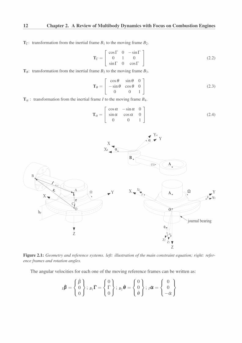
2.3 Mathematical modelling of reciprocating machinesBased on multibody dynamics theory, the formulation of representative motion equations that de-scribe the dynamics of a slider crank mechanism in a typical reciprocating machine is presentedin this section. These equations will be further coupled to the dynamics of the fluid film bearings,which will be described in chapter 5. In the model, connecting rod and crank are considered as rigidbodies, and piston motion is modelled as a particle. Three different approaches were considered inorder to account for the reaction forces at the crank-rotor connection. The three cases differ in thedefinition of the restrictive conditions of motion of the centre of the crank:
• Case (I). Considering a rigid crank bearing model. This is the most simple case, in whichcrank is only allowed to rotate, neglecting lateral displacements and tilting oscillations of thecrank.
• Case (II). Considering a rigid crankshaft model. In this case, the crank is allowed to havelateral displacements but not tilting oscillations. In other words, the crankshaft is consideredrigid and supported by fluid film bearings.
• Case (III). Considering a flexible crankshaft model. In this case, the crank is allowed to havelateral displacements and tilting oscillations. Similarly to case (II), reaction forces at thecrank-rotor connection are given by the dynamics of the bearing fluid film, but in this case therotor (crankshaft) is considered flexible and will be modelled using finite elements.
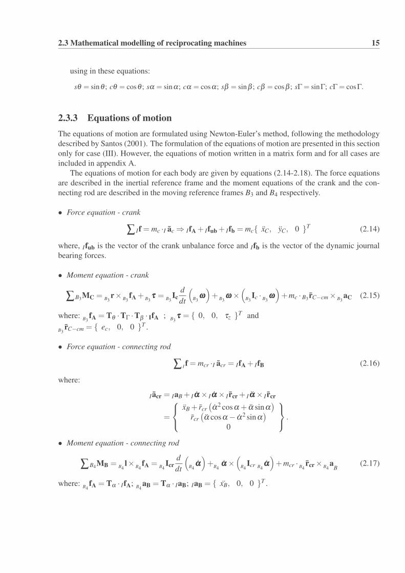
For each one of the three cases, the motion equations for the piston-connecting rod-crank systemare formulated with the help of MBD theory, using the Newton-Euler’s method and using a framenotation of common use in multibody dynamics (Bremer, 1988; Ulbrich, 1996; Santos, 2001). Fig-ure 2.1 is a sketch representing the main geometric characteristics of the system, indicating referenceframes and main angles of rotation (β , Γ, θ and α).
2.3.1 Inertial and moving reference framesIn order to be able to describe all the representative vectors, one inertial reference frame (IXY Z) andfour moving reference frames (Bi) were defined. The inertial reference frame is attached to the cen-ter of the bearing (point O), the moving reference frames B1(X1Y1Z1), B2(X2Y2Z2) and B3(X3Y3Z3)are attached to the crank and the moving reference frame B4(X4Y4Z4) is attached to the connectingrod. Thus, B1 (X1Y1Z1) is obtained by rotating I the angle β , around the X axis; B2 (X2Y2Z2) isobtained by rotating B1 the angle Γ, around the Y1 axis; B3 (X3Y3Z3) is obtained by rotating B2 theangle θ , around the Z2 axis; B4 (X4Y4Z4) is obtained by rotating I the angle α , around the Z axis.With the help of the geometric transformation matrices Tβ , TΓ, Tθ and Tα any vector can be easilytransformed from one reference frame to another. The transformation matrices are given by:
Tβ : transformation from the inertial frame I to the moving frame B1.
Tβ =
⎡⎣ 1 0 0
0 cosβ sinβ0 −sinβ cosβ
⎤⎦ (2.1)
12 Chapter 2. A Review of Multibody Dynamics with Focus on Combustion Engines
TΓ: transformation from the inertial frame B1 to the moving frame B2.
TΓ =
⎡⎣ cosΓ 0 −sinΓ
0 1 0sinΓ 0 cosΓ
⎤⎦ (2.2)
Tθ : transformation from the inertial frame B2 to the moving frame B3.
Tθ =
⎡⎣ cosθ sinθ 0
−sinθ cosθ 00 0 1
⎤⎦ (2.3)
Tα : transformation from the inertial frame I to the moving frame B4.
Tα =
⎡⎣ cosα −sinα 0
sinα cosα 00 0 1
⎤⎦ (2.4)
Figure 2.1: Geometry and reference systems. left: illustration of the main constraint equation; right: refer-
ence frames and rotation angles.
The angular velocities for each one of the moving reference frames can be written as:
Iβββ =
⎧⎨⎩
β00
⎫⎬⎭ ; B1ΓΓΓ =
⎧⎨⎩
0Γ0
⎫⎬⎭ ; B2 θθθ =
⎧⎨⎩
00θ
⎫⎬⎭ ; Iααα =
⎧⎨⎩
00−α
⎫⎬⎭

2.3 Mathematical modelling of reciprocating machines 13
2.3.2 Constraint equations and kinematic equations
A different constraint equation will be established for each one of the three cases considered. Theexpressions to calculate velocities and accelerations of the piston (xB, xB) and the connecting rod(α , α), are obtained by differentiating once and twice the constraint equation given for each case.
The absolute angular velocity of the crank (ωωω), written with help of the moving reference frameB3, is given by:
B3ωωω = B3 βββ + B3ΓΓΓ+ B3 θθθ (2.5)where:
B3 βββ = Tθ TΓTβ Iβββ
B3ΓΓΓ = Tθ TΓ B1ΓΓΓ
B3 θθθ = Tθ B2 θθθ
Since in cases (I) and (II), the tilting oscillations of the crank are not considered (i.e., β and Γare equal to zero), the transformation matrices B1 and B2 are not required, and the moving referenceframe B3 will be simply obtained by rotating I the angle θ , around the Z axis. Thus, in these twocases the absolute angular velocity of the crank is simplified to: B3ωωω = {0 0 θ}T , where θ is alsoequal to Ω.
Case (I)
• Main constraint equation:
Ixp + Il = Ir (2.6)
where,Ir = TT
θ · B3r
B3r ={
rc 0 −hp
}T
Il ={ −l cosα l sinα 0
}T
Ixp ={
xB 0 −hp
}T
• Velocities: [1 l sinα0 l cosα
]{xB
α
}=
{ −rcθ sinθrcθ cosθ
}(2.7)
• Accelerations: [1 l sinα0 l cosα
]{xB
α
}=
{ −rc(θ sinθ − θ 2 cosθ)− lα2 cosαrc(θ cosθ − θ 2 sinθ)+ lα2 sinα
}(2.8)

14 Chapter 2. A Review of Multibody Dynamics with Focus on Combustion Engines
Case (II)
• Main constraint equation:Ixp + Il = Ir+ Ic (2.9)
where, Ic ={
xC yC 0}T .
• Velocities: [1 l sinα0 l cosα
]{xB
α
}=
{ −rcθ sinθ + xC
rcθ cosθ + yC
}(2.10)
• Accelerations:[1 l sinα0 l cosα
]{xB
α
}=
{ −rc(θ sinθ − θ 2 cosθ)− lα2 cosα + xC
rc(θ cosθ − θ 2 sinθ)+ lα2 sinα + yC
}(2.11)
Case (III)
• Main constraint equation.In this case the main constraint equation is also given by Eq. (2.9), but due to the rotations in β andΓ, vector Ir is obtained by:
Ir = TTβ ·TT
Γ ·TTθ · B3r
• Velocities: [1 l sinα0 l cosα
]{xB
α
}=
{k1k2
}(2.12)
• Accelerations: [1 l sinα0 l cosα
]{xB
α
}=
{k3k4
}(2.13)
where:
k1 = −rc(ΓsΓcθ + θcΓsθ)−hpΓcΓ+ xC
k2 = rcβ (cβ sΓcθ − sβ sθ)+ rcθ(cβcθ − sβ sΓsθ)+Γ(rcsβcΓcθ −hpsβ sΓ)+ βhpcβcΓ+ yC
k3 = −rcΓsΓcθ + Γ2(hpsΓ− rccΓcθ)+2rcθ ΓsΓsθ−rcθ 2cΓcθ −hpΓcΓ− rcθcΓsθ − lα2cα + xC
k4 = −rcθ 2(cβ sθ + sβ sΓcθ)− β 2(rccβ sθ + rcsβ sΓcθ +hpsβcΓ)−Γ2(rcsβ sΓcθ +hpsβcΓ)+ β (hpcβcΓ− rcsβ sθ + rccβ sΓcθ)+Γ(rcsβcΓcθ −hpsβ sΓ)−2rcθ β (sβcθ + cβ sΓsθ)+2β Γ(rccβcΓcθ −hpcβ sΓ)−2rcθ ΓsβcΓsθ+rcθ(cβcθ − sβ sΓsθ)+ lα2sα + yC
2.3 Mathematical modelling of reciprocating machines 15
using in these equations:
sθ = sinθ ; cθ = cosθ ; sα = sinα; cα = cosα; sβ = sinβ ; cβ = cosβ ; sΓ = sinΓ; cΓ = cosΓ.
2.3.3 Equations of motionThe equations of motion are formulated using Newton-Euler’s method, following the methodologydescribed by Santos (2001). The formulation of the equations of motion are presented in this sectiononly for case (III). However, the equations of motion written in a matrix form and for all cases areincluded in appendix A.
The equations of motion for each body are given by equations (2.14-2.18). The force equationsare described in the inertial reference frame and the moment equations of the crank and the con-necting rod are described in the moving reference frames B3 and B4 respectively.
• Force equation - crank
∑ If = mc ·I ac ⇒ IfA + Ifub + Ifb = mc{ xC, yC, 0 }T (2.14)
where, Ifub is the vector of the crank unbalance force and Ifb is the vector of the dynamic journalbearing forces.
• Moment equation - crank
∑B3MC =B3
r×B3
fA +B3
τττ =B3
Icd
dt
(B3
ωωω)+
B3ωωω ×
(B3
Ic · B3ωωω
)+mc · B3 rC−cm ×
B3aC (2.15)
where:B3
fA = Tθ ·TΓ ·Tβ · IfA ;B3
τττ = { 0, 0, τz }T and
B3rC−cm = { ec, 0, 0 }T .
• Force equation - connecting rod
∑ If = mcr ·I acr = IfA + IfB (2.16)
where:
I acr = IaB + Iααα × Iααα × I rcr + Iααα × I rcr
=
⎧⎨⎩
xB + rcr
(α2 cosα + α sinα
)rcr
(α cosα − α2 sinα
)0
⎫⎬⎭ .
• Moment equation - connecting rod
∑B4MB =B4
l×B4
fA =B4
Icrd
dt
(B4
ααα)+
B4ααα ×
(B4
Icr B4ααα
)+mcr · B4
rcr × B4a
B(2.17)
where:B4
fA = Tα · IfA;B4
aB = Tα · IaB; IaB = { xB, 0, 0 }T .

16 Chapter 2. A Review of Multibody Dynamics with Focus on Combustion Engines
• Force equation - piston
∑ IfB = mp ·I aB = IfB + IfN + Ifp (2.18)
where: Ifp = { PgAp, 0, 0 }T .
The equations of motion can be rewritten in a matrix form as in Eq. (2.19), where the vector bcontains the main unknowns of the system (e.g., reaction forces, reaction moments and accelera-tions). This matrix system is fully described for each case in appendix A.
A · b = c (2.19)
where the vector b for each case is given by:
b(I) = { fBx , fBy , fBz , Ny, Nz, fAx, fAy
, fAz, fCx
, fCy, fCz
, MCx, MCy
, θ , xB, α}T
b(II) = { fBx , fBy , fBz , Ny, Nz, fAx, fAy
, fAz, fCz
, Mcx , Mcy , θ , xB, α, xC, yC}T
b(III) = { fBx , fBy , fBz , Ny, Nz, fAx, fAy
, fAz, fCz
, θ , xB, α, xC, yC, β , Γ}T
2.3.4 Modelling of the rotorIn order to account for lateral displacements and tilting oscillations of the crankshaft, as defined forcase (III), the crankshaft is modelled as a flexible body using a finite elements formulation wherethe rotor bearing system is assumed to be supported by flexible supports, and the gyroscopic androtational inertia effects are included, as described by Nelson and McVaugh (1976). Thus, the globalequation of motion for the rotor, described in the inertial reference frame I can be written as:
M · q = f− G · q− K ·q︸ ︷︷ ︸f
(2.20)
where, M, K and G are the mass, stiffness and gyroscopic matrices respectively; f is the vector ofloads acting on the rotor, given by: I f =I fpl +I fub +I fb, where Ifpl is the vector of static preloadforces, Ifub is the vector of unbalance rotor forces, and Ifb is the vector that contains the hydro-dynamic bearing forces. In a journal bearing, the fluid film forces are strongly dependent on thedynamics of the journal. These forces will be calculated based on the theory of hydrodynamic lu-brication, using analytical and numerical solutions of Reynolds equation, as detailed in the nextchapter.
The flexibility of the crankshaft is coupled to the MBD model of the reciprocating mechanismthrough equations. Thus, the matrix system given by Eq. (2.19) will be coupled to the equationsof the finite elements formulation of the rotor in the degrees of freedom where crank and rotor areconnected, which is further explained in chapter 5.

Chapter 3
Dynamically Loaded Journal Bearings -DLJBs
3.1 Modelling approaches
Fluid film bearings have a strong influence on the dynamics of rotor-bearing systems, which madethem the focus of numerous studies over the years. One of the earliest attempts to model fluid filmbearings was reported by Stodola in 1925, who investigated the effect of oil-film stiffness on thecritical speed of a shaft supported in hydrodynamic journal bearings (Sawicki et al., 1997). Like-wise, the dynamic performance of reciprocating machinery can be significantly influenced by thedynamics of their bearing supports. Therefore, fluid film bearings under dynamic load conditionshave been a matter of concern of numerous theoretical and experimental investigations over the lastforty years (Campbell et al., 1967-1968; Martin, 1983; Xu, 1999; Goodwin et al., 2003). The mobil-ity technique, developed by Booker (1965), was one of the earliest approaches and one of the mostcommon methods used for the analysis of DLBs. The analysis of DLJBs, based on the assumptionof a rigid bearing model, can be satisfactory in cases where only a parametric analysis is required, orin cases where the elastic deformations expected are not significant (Oh and Goenka, 1985). Nev-ertheless, other methods involving flexibility and thermal effects, but with higher computationalcomplexity, have been developed during the past three decades.
In reality, bearings and housings are flexible to a certain degree, especially in the new genera-tion of machines, which are required to work at higher speeds and under heavier load conditions,they weight less and are more flexible. Therefore, in order to account for elastic deformations,corrections are now being made by using elasto-hydrodynamic theory EHD, combined with FEMmodels of bearings and housing. However, in spite of the nowadays availability of highly efficientcomputational resources, the substantial increase in computation time required to perform an EHDanalysis is still considered a main drawback. In practice, EHD calculations are presently done onlyin special cases (Subramanyan, 2000; Fridman et al., 2004), but are on the way to become standardin the routine bearing analysis. A summary of selected studies using EHD lubrication theory forthe analysis of engine bearings is given in the study by Moreau et al. (2002).
In some cases of engine bearing analysis (e.g., heavily loaded main bearings and connecting rodbearings) a thermo-hydrodynamic analysis (THD ) may be required, since the influence of thermal
17

18 Chapter 3. Dynamically Loaded Journal Bearings - DLJBs
effects on the hydrodynamic pressure generation and consequently on the value of journal eccen-tricity may be significant (Fatu et al., 2006). However, it has to be considered that THD analysisinvolves the simultaneous solution of Reynolds equation, energy and heat transfer equations, whichdemands high computational cost and efforts to develop.
The study of the variation of stiffness and damping coefficients in the analysis of DLJB, par-ticularly crankshaft bearings, is commonly avoided due to the computational cost and lack of non-reliable close-forms of solutions, however, some studies have proposed simplified methodologies toevaluate stiffness and damping coefficients over a load cycle based on SJB and LJB approximations,as in the work of Hirani et al. (1999a).
A review of theoretical and experimental studies related to design and performance assessmentof bearings in reciprocating machinery was carried out by Goodwin et al. (2003). It was foundsignificant disagreement between theoretical and experimental results, by making a comparison be-tween the theoretically predicted and the experimentally measured eccentricities. Such a disagree-ment is on one side caused by the several limitations found in the experimental methods referredin that study, and on the other side, caused by the comparison of experimental results to theoreticalresults obtained from well detailed and sometimes complex theoretical models for DLJBs. Thus, inmany cases the use of simplified bearing models may be good enough to represent and understandthe physics of the problem, and to obtain numerical results comparable to the experimental ones.In fact, one of the main conclusions drawn by Goodwin et al. (2003), is that in many cases, a shortbearing approximation can be used with good accuracy for the purpose of modelling oil film pres-sure, without the need of using more sophisticated models. Some of the previous studies relatedto theoretical modelling and experimental methods to analyze DLJB, cited also by Goodwin are:Booker (1965), Campbell et al. (1967-1968), Warner (1963), Ross and Slaymaker (1969), Ritchie(1975), Martin (1983), Fantino and Frene (1985), Goenka and Oh (1986), Pal et al. (1988), Goenkaand Paranjpe (1992), Choi et al. (1992), Knoll et al. (1997), Xu (1999). A summary of relevantstudies related to the analysis of DLJB is given in Table 3.1. It is worth noting that the list of pub-lished works related to the theoretical and experimental treatment of DLJBs is extensive, therefore,not all of them are mentioned in Table 3.1.
3.2 Tribology of engine bearingsIn a typical ICE, the crankshaft is supported by journal bearings, as illustrated in Fig. 3.1a. Thesebearings, which are also known as main bearings, are commonly designed to operate in the hy-drodynamic regime of lubrication even under the most extreme conditions of load and speed en-countered in an operating engine. The analysis of engine bearings can be rather complicated sincetheir tribological behaviour can be influenced by factors such as lubricant supply, thermal effects,dynamic loading and elasticity of the bounding solids (Tung and McMillan, 2004). The most im-portant components that contribute to the mechanical friction losses in reciprocating engines areindicated in Fig. 3.1b. The lubricant films surrounding the main bearings support the inertial loadof the crankshaft and the combustion forces transmitted from the cylinders to the crankshaft. Theseforces are periodic, but depending on the working load and speed conditions of the engine, they maychange in magnitude from one cycle to the next, generating vibrations of the journal centre due to

3.2 Tribology of engine bearings 19
the combined action of rotating inertias and reciprocating forces.

20 Chapter 3. Dynamically Loaded Journal Bearings - DLJBs
Table 3.1: Review of literature - Studies on the modelling of dynamically loaded journal bearings (DLJBs).
Year Author Overview
1965 Booker Mobility maps, describing the journal force/velocity relationships at differ-ent eccentricities at attitude angles are investigated.
1967-1968
Campbell et al. Mobility method is compared to approximate methods. These methodsmade use of a quasi-static analysis based on an ’equivalent speed’ witha constant load and made use of bearing loads estimated on the basis ofinertia forces only, using SJB, FJB and LJB solutions. Comparisons be-tween theoretical and experimental results for the big-end journal bearingof a diesel engine running at 600rpm are presented.
1969 Ross and Slaymaker Bearing orbits based in Ocvirk’s SJB approximation. This paper showsthat, for small length/diameter ratio bearings, the Ocvirk solution yieldsgood prediction of bearing orbital motion.
1972 Craven and Holmes A computational method based on SJB analysis, using Newton iterationand variation of the trapezium rule is developed.
1975 Ritchie An optimized SJB solution is presented. First attempt to reconcile the ad-vantages of an approximate solution with the accuracy of a full bearingsolution.
1983 Martin Review of work undertaken mainly concerned with oil film history, inertiaeffects, bearing non-circularity, bearing flexibility and lubricant supply portgeometry.
1985 Fantino and Frene EHD analysis using SJB theory. Journal trajectories are published in thispaper.
1985 Oh and Goenka Results compared to data for a rigid bearing. It was conclude that a fullEHD analysis is necessary for an accurate prediction of engine bearingperformance, but that this involves a substantial increase in computationtime. A rigid bearing model is satisfactory if only a parametric analysis isrequired.
1989 White Analysis of orbits obtained for journal bearings (using a FJB solution) of adiesel engine, and a two-stage reciprocating compressor.
1992 Goenka and Paranjpe Several methods used in General Motors for engine bearing analysis are re-viewed. The implications of using the Sommerfeld and Reynolds boundaryconditions were discussed. A finite volume method for identifying cavita-tion zones is described.
1992 Choi et al. Theoretical analysis using the SJB theory and the mobility method. Itwas observed that crankshaft vibrations and the unbalance between thecrankshaft bearings have a large influence on the minimum oil film thick-ness (OFT ). Minimum OFT occurred during either the exhaust or com-pression strokes when piston and connecting rod inertia forces are domi-nant, and it decreased almost linearly with engine speed and did not changesignificantly with engine load.
1996 Vincent et al. A numerical investigation of cavitation in DLJB using the mobility methodwas presented and a comparison of results using the cavitation formulationof Elrod was made.
1996 Paranjpe The performance of main bearings and connecting rod bearings is studiedusing a full THD analysis, an adiabatic THD analysis and a simplifiedthermal analysis.
1997 Knoll et al. Reynolds equation is solved for the oil film pressure profile in main bear-ings using the FEM method. This model separates the complete structuredisplacement into a large rigid body and small elastic deformations.

3.2 Tribology of engine bearings 21
continuation of Table 3.1
1998 Hirani et al. A semi-analytical procedure to evaluate pressure and minimum OFT con-sidering a finite bearing is presented in this paper. Using the methodologyproposed for two cases of engine bearings, the results obtained are com-pared in terms of computational time and accuracy with the short bearingapproximation and finite element analysis respectively.
1999b Hirani et al. A ’closed-form’ expression of the pressure distribution for DLJB is pro-posed. This expression is based on a combination of SJB and LJB approx-imations. An analytical method for evaluating the angular location of theinstantaneous maximum pressure is provided. The study is validated ana-lyzing a connecting rod big end bearing and two crankshaft main bearings.
1999 Xu The use of EHD theory to the engine bearing analysis is highlighted as asignificant tool for the understanding of engine bearings.
2000 Lahmar et al. An optimised SJB theory was proposed and applied for nonlinear dynamicanalysis of finite-width journal bearings supporting an unbalanced rigid ro-tor.
2002 Moreau et al. Comparison of theoretical calculations (using EHD theory) and experimen-tal measurements of OFT in a dynamically loaded crankshaft main bearing.A short review of previous theoretical and experimental studies is included.
2003 Goodwin et al. A significant disagreement between published theoretical and experimentaldata still remains, in spite of the use of more sophisticated theoretical mod-els. There is a general consensus that a short bearing approximation can beused with good accuracy for the purposes of modelling oil film pressure,although the modelling techniques and computing power available nowa-days, also permit full bearing solutions.
2005 Alshaer et al. A generalized model for a lubricated long journal bearing in a MBD modelof a slider-crank mechanism is presented, where the lubricated journal bear-ing under study is given by the joint between connecting rod and slider.Orbits and reaction moments are obtained and analyzed.
2006 Fatu et al. A thermo-elasto-hydrodynamic (TEHD ) lubrication analysis of a big-endconnecting rod bearing is carried out in this study. Thermal distortionsand elastic deformation of the bearing surfaces are computed using FEMmethod. The change of oil viscosity with temperature is also taken intoaccount.
2007 Bukovnik et al. In this work several crankshaft main bearings and connecting rod big endbearings are investigated. Comparisons between results obtained by us-ing clasical methods and complex numerical methods, such as EHD andTEHD, are presented. The simulations are performed using the comercialsoftware EXCITE.
2008 Backhaus and Knoll This paper describes a simulation software that was developed to improvecalculations of oil supply to plain engine bearings, based on an EHD anal-ysis.
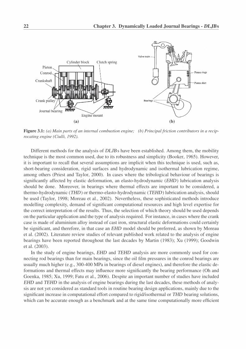
22 Chapter 3. Dynamically Loaded Journal Bearings - DLJBs
(a) (b)
Figure 3.1: (a) Main parts of an internal combustion engine; (b) Principal friction contributors in a recip-
rocating engine (Ciulli, 1992).
Different methods for the analysis of DLJBs have been established. Among them, the mobilitytechnique is the most common used, due to its robustness and simplicity (Booker, 1965). However,it is important to recall that several assumptions are implicit when this technique is used, such as,short-bearing consideration, rigid surfaces and hydrodynamic and isothermal lubrication regime,among others (Priest and Taylor, 2000). In cases where the tribological behaviour of bearings issignificantly affected by elastic deformation, an elasto-hydrodynamic (EHD ) lubrication analysisshould be done. Moreover, in bearings where thermal effects are important to be considered, athermo-hydrodynamic (THD ) or thermo-elasto-hydrodynamic (TEHD ) lubrication analysis, shouldbe used (Taylor, 1998; Moreau et al., 2002). Nevertheless, these sophisticated methods introducemodelling complexity, demand of significant computational resources and high level expertise forthe correct interpretation of the results. Thus, the selection of which theory should be used dependson the particular application and the type of analysis required. For instance, in cases where the crankcase is made of aluminium alloy instead of cast iron, structural elastic deformations could certainlybe significant, and therefore, in that case an EHD model should be preferred, as shown by Moreauet al. (2002). Literature review studies of relevant published work related to the analysis of enginebearings have been reported throughout the last decades by Martin (1983); Xu (1999); Goodwinet al. (2003).
In the study of engine bearings, EHD and TEHD analysis are more commonly used for con-necting rod bearings than for main bearings, since the oil film pressures in the conrod bearings areusually much higher (e.g., 300-400 MPa in bearings of diesel engines), and therefore the elastic de-formations and thermal effects may influence more significantly the bearing performance (Oh andGoenka, 1985; Xu, 1999; Fatu et al., 2006). Despite an important number of studies have includedEHD and TEHD in the analysis of engine bearings during the last decades, these methods of analy-sis are not yet considered as standard tools in routine bearing design applications, mainly due to thesignificant increase in computational effort compared to rigid/isothermal or THD bearing solutions,which can be accurate enough as a benchmark and at the same time computationally more efficient

3.3 Mathematical modelling of dynamically loaded fluid film bearings 23
(Fridman et al., 2004). Nevertheless, EHD and TEHD analysis are increasingly being used, and arerapidly on the way to become of common use in bearing design, as it can be seen, in the studiesof MAN B&W Diesel A/S (2002); Makino and Koga (2002); Bukovnik et al. (2006, 2007); AVL(2009).
The study of actively lubricated engine bearings using EHD or TEHD analysis can make theproblem computationally prohibitive, considering that the hydrodynamics of the oil films has to becoupled to the dynamics of the oil injection. Additionaly, in reciprocating machines such as ICEs,the lubrication problem should be coupled to the dynamics of the piston-connecting rod assembly(which accounts for the acting loads coming from the combustion forces and the inertia of the me-chanical components), adding complexity to the modelling. Hence, in this work, the use of EHDand TEHD analysis were not considered for the analysis of main engine bearings. It is worth tomention that the main focus of this study is on the evaluation of main bearings performance operat-ing under controllable lubrication conditions, rather than on the estimation of elastic deformationsof mechanical components. Thus, a rigid isothermal finite-bearing approach was adopted, assum-ing a hydrodynamic regime of lubrication and using a computationally efficient but yet accurateanalysis, which is detailed in the next sections. Other investigations on tilting pad journal bear-ings using EHD analysis Haugaard and Santos (2009), theoretical and experimental THD analysisSantos and Nicoletti (1999, 2001), and TEHD analysis Heinrichson et al. (2007); Heinrichson andSantos (2008), can be found in the literature.
3.3 Mathematical modelling of dynamically loaded fluid filmbearings
The governing equations of the dynamics of the thin fluid film in conventionally lubricated journalbearings operating under dynamic load conditions, are presented in this section. The main geometricrelations and reference frames for a DLJB are shown in Fig. 3.2.
Figure 3.2: Journal bearing geometry.
The equation that describes the oil flow in a journal bearing in the domain 0 ≤ x ≤ 2πrb and−lb/2 ≤ z ≤ lb/2, and which governs the pressure distribution of the oil film can be obtained from

24 Chapter 3. Dynamically Loaded Journal Bearings - DLJBs
the standard reduced form of the Reynolds equation for fluid film lubrication (Hamrock, 1991),given by:
∂∂x
(ρh3
12μ∂ p
∂x
)+
∂∂ z
(ρh3
12μ∂ p
∂ z
)=
∂∂x
(ρh(Uj −Ub)
2
)+
∂ (ρh)
∂ t(3.1)
Equation (3.1) describes the pressure distribution p(x,z, t) between rotor and sleeve, as a func-tion of the oil properties (ρ,μ), the relative velocity between rotor and sleeve surfaces (Uj −Ub),and the gap function h(x,z, t). The gap function defines the profile of the OFT around the bearing.Assuming that the fluid is isoviscous, Newtonian and incompressible, and considering a typical casewhere the journal rotates and the sleeve remains stationary (i.e., Uj =Ωrb and Ub = 0), the Reynoldsequation for hydrodynamic lubrication can be written as
∂∂x
(h3 ∂ p
∂x
)+
∂∂ z
(h3 ∂ p
∂ z
)= 6μUj
∂h
∂x+12μ
∂h
∂ t(3.2)
With reference to the diagram in Fig. 3.2, the gap function can be written as
h = cb(1+ ε cosϕ) (3.3)
where ϕ is the angle measured from the location of the maximum OFT, cb is the radial clearance,and ε is the eccentricity ratio, given by ε = eb/cb. Using the coordinate transformation x = rbϕ ,where rb is the bearing radius, and introducing Eq. (3.3) in the right hand side of Eq. (3.2), themodified Reynolds equation for DLJB can be written as
∂∂ϕ
(h3 ∂ p
∂ϕ
)+ rb
2 ∂∂ z
(h3 ∂ p
∂ z
)= 12μcbrb
2[
ε cosϕ + ε sinϕ(φ − Ω2)
](3.4)
or alternatively as:
3h2 ∂h
∂ϕ∂ p
∂ϕ+h3 ∂ 2 p
∂ϕ2 + rb2h3 ∂ 2 p
∂ z2 = 12μcbrb2[
ε cosϕ + ε sinϕ(φ − Ω2)
](3.5)
where, ε corresponds to the normal squeeze velocity of the oil film, φ is the rotational velocity ofthe journal centre around the bearing centre, Ω is the rotational speed of the rotor, and ∂h/∂ϕ =−eb sinϕ . Equation 3.5 can be used when misalignment is not considered, in other words, whenOFT is assumed to be constant along the width direction of the bearing. Since the eccentricity andattitude angle in a DLJB change through the loading cycle, Eq. (3.5) can only be solved if (ε , φ andΩ) are known at any time during each cycle.
3.3.1 Analytical solutions of Reynolds equationAcceptable analytical solutions of Eq. (3.4) can be obtained for limited cases, such as, short-width(SJB) and infinitely long-width (LJB) journal bearings (Frene et al., 1990; Hamrock, 1991). Someattempts to develop analytical or so called ’close-form’ solutions of Reynolds equation for finite-width DLJB were proposed by Hirani et al. (1999b,a). However, their use is not widely extended,and numerical solutions are still preferred. In the SJB approach, it is considered that the variation

3.3 Mathematical modelling of dynamically loaded fluid film bearings 25
of film pressure is more significant in the axial direction than in the circumferential direction, ne-glecting the first term on the left hand side of Eq. (3.4). The use of this approach is suitable forbearings with small aspect ratio (λ ≤ 0.5) operating with small to moderate eccentricity (ε ≤ 0.75).Since engine bearings are usually of short-width dimensions, this approach is commonly used fortheir analysis. By contrast, the LJB approach considers that the film pressure is constant along theaxial direction, and therefore, the side-leakage term, i.e., the second term on the left hand side ofEq. (3.4) can be disregarded. The analytical solutions obtained with the LJB approach may be usedfor the analysis of long-width bearings (usually λ > 2). Since LJB are proned to misalignment, thisapproach is hardly used in common practice.
Analytical solutions for SJB and LJB approximations
Assuming that the bearing is well aligned and the viscosity of the lubricant keeps constant, andusing the Gumbel boundary conditions, the reduced Reynolds equation for the SJB and the LJBapproaches can be analytically integrated, obtaining the expressions given by Eqs. (3.6) and (3.7),respectively (Frene et al., 1990). For each case, the journal bearing forces given in ξ ,η coordinates(see Fig. 3.2) can be calculated integrating the pressure distribution along the bearing surface, as inEq. (3.8), obtaining the analytical expressions listed in Table 3.2.
pSJB
= −3μh3
(lb
2
4− z2
)[(Ω−2φ)
∂h
∂ϕ+2εcb cosϕ
](3.6)
pLJB
= 6μ(
rb
cb
)2 {(Ω−2φ)
ε sinϕ(2+ ε cosϕ)(2+ ε2)(1+ ε cosϕ)2 +
εε
[1
(1+ ε cosϕ)2 −1
(1+ ε)2
]}(3.7)
{fξfη
}=
∫ 2π
0
∫ lb
0p
{cosϕsinϕ
}rbdzdϕ (3.8)
Table 3.2: Analytical solutions of Reynolds equation to calculate journal bearing forces (Frene et al., 1990).
• Short-width journal bearing (SJB )
fξ = −rbμlb3
2cb2(1−ε2)2
[πε(1+2ε2)√
(1−ε2)+2ε2(Ω−2φ)
]
fη = rbμlb3ε
2cb2(1−ε2)2
[4ε + π
2 (Ω−2φ)√
1− ε2]
• Long-width journal bearing (LJB )
fξ = −12μrb3lb
cb2
[ε2(Ω−2φ)
(2+ε2)(1−ε2)+ ε
(1−ε2)3/2
(π2 − 8
π(2+ε2)
)]fη = 12μrb
3lbcb
2
[πε(Ω−2φ)
2(2+ε2)√
1−ε2 +2εε
(2+ε2)(1−ε2)
]
26 Chapter 3. Dynamically Loaded Journal Bearings - DLJBs
Viscous friction forces
The instantaneous viscous frictional forces acting in the opposite direction of the sleeve rotation canbe obtained by integrating the shear stress around the journal surface:
fv f =∫
sλ ∗
xyrbdϕdz (3.9)
where the fluid shear stress is given by λxy = μ∂ux/∂y and ux is obtained from Navier-Stokesequation, and it is given as a function of the pressure field by:
ux =1
2μ∂ p
∂xy(y−h)+
rbΩy
h(3.10)
∂ux
∂y=
12μ
∂ p
∂x(2y−h)+
rbΩh
(3.11)
Thus, the fluid shear stress calculated along the journal surface (y = h), is given by:
λ ∗xy =
μrbΩh
+h
2rb
d p
dϕ.
In dimensionless form, the friction force can be written as:
fv f =fv f
μΩr2C
lb(3.12)
The friction coefficient is defined as the ratio of the friction force and the bearing load capacity.In dimensionless form (number of friction), is given by:
μ f =fv f
Fb
rb
C(3.13)
where Fb is the instantaneous bearing load capacity, calculated by: Fb =√
Fξ2 +Fη
2. The in-stantaneous power dissipation caused by viscous frictional forces and the cyclic averaged powerconsumption can be written as:
Wv f = Ω · rb · fv f (3.14)
(Wv f )avg=
12π
∫ 2π
0Wf dθ (3.15)
3.3.2 Numerical solution of Reynolds equationAnalytical and rapid procedures for oil film calculation, such as those based on the mobility method(Booker, 1965), cannot adequately take into account the influence of features in the bearing suchas oil holes and grooves, since the solution assumes an uninterrupted oil film. Therefore, in caseswhere a FJB approach is required, the 2D Reynolds equation has to be numerically solved. Usingnumerical methods for bearing analysis enables additional possibilities, such as, including elastic

3.3 Mathematical modelling of dynamically loaded fluid film bearings 27
and thermo-elastic effects (Kim and Kim, 2001; Fatu et al., 2006), compressibility, piezoviscos-ity effects and non-Newtonian fluid behaviour. Typical numerical schemes used for the solutionof Reynolds equation are based on the finite elements method - FEM (Reddi, 1969; Booker andHuebner, 1972), finite difference method - FD (Mitsui, 1988) and finite volumes. In this work, aFD scheme with the assumption of isothermal conditions (Santos and Russo, 1998), was adopted,which is described next for completeness and to establish notation.
Finite difference scheme with a uniform mesh
In this case, the Reynolds equation is discretized via finite differences using an uniform mesh ofm×n nodes along ϕ and z directions, as shown in Fig. 3.3. Using a central difference scheme, andneglecting second and higher order terms, the first and second order derivatives can be written as:
Figure 3.3: Uniform finite difference mesh.
∂ p
∂ϕ
∣∣∣∣m,n
=pm+1,n − pm−1,n
2Δϕ(3.16)
∂ 2 p
∂ϕ2
∣∣∣∣m,n
=pm+1,n −2pm,n + pm−1,n
Δϕ2 (3.17)
Assuming that the bearing is well aligned (i.e., ∂h/∂ z = 0), and the viscosity of the fluid film keepsconstant, the Reynolds equation written in finite differences is given by:
Δm,n pm−1,n +Λm,n pm+1,n+♦m,n pm,n +∇m,n pm,n−1 +�m,n pm,n+1
= 12μcbrb2[
ε cosϕm,n + ε sinϕm,n(φ − Ω2)
](3.18)
where,
Δm,n =−3h2m,n
2Δϕ∂h∂ϕ
∣∣∣m,n
+h3
m,n
Δϕ2 ; Λm,n =3h2
m,n
2Δϕ∂h∂ϕ
∣∣∣m,n
+h3
m,n
Δϕ2
♦m,n =−2h3m,n
[1
Δϕ2 +r2
b
Δz2
]; ∇m,n =�m,n =
h3m,nr2
b
Δz2

28 Chapter 3. Dynamically Loaded Journal Bearings - DLJBs
The boundary conditions that are applied for the numerical solution of Eq. (3.18) are: p(z= 0) =0 and p(z = lb) = 0 (i.e., boundary pressure at the bearing edges is atmospheric); p(ϕ = 0) = 0and p(ϕ = 2π) = 0, considering maximum film pressures close to the location of the minimumOFT ; p ≥= 0, assuming the Gumbel boundary cavitation condition.
The discretized Reynolds equations is solved for each time step by using a direct system equationsolver based on the well known LU factorization method (Wendt, 1992). Once the nodal pressureshave been computed, the resultant forces on the sleeve are obtained by numerically integratingEq. (3.8), for instance, using the Simpson Method.
3.3.3 Boundary conditions and cavitation approachesThe analytical solution for the oil film pressure distribution can be obtained when adequate boundaryconditions (BC ) are applied for the integration of Reynolds equation, when using SJB and LJB
approximations. The most known boundary conditions for the analytical solutions of the Reynoldsequation for DLJB are: Full Sommerfeld conditions, Half Sommerfeld conditions and Gumbelboundary conditions.
• Full Sommerfeld solution is a periodic boundary condition, which assumes that the pressuresat edges of the wedge is equal to zero, i.e., p = 0, at ϕ = 0 and ϕ = 2π . Since applying thiscondition large negative pressures occur in the diverging zone, it is not used in practice.
• Half Sommerfeld solution is a more realistic approach, which disregards negative pressuresin the diverging area, i.e., p = 0, at ϕ = 0; p = 0 at ϕ = π/2; p = 0 at π/2 < ϕ < 2π . Al-though this boundary condition does not conserve the continuity of flow, which is physicallyunrealistic, it is simple to apply and can be accurate enough in many cases.
• Gumbel cavitation condition is another well known cavitation condition, in which the Reynoldsequation is first solved subjected to the specified pressures at the bearing boundaries, and thenif subambient pressures appear they are disregarded. Although the use of the Gumbel cavita-tion condition does not satisfy the continuity of flow at film rupture as well as reformation, itprovides acceptable accuracy in the estimation of oil film pressure and bearing load capacitywith low computational cost (Mourelatos, 2001b).
When numerical solutions are used, more accurate boundary cavitation conditions can be adopted,such as, the Reynolds or Swift-Stieber conditions, and the Jackobsson-Floberg and Olson (JFO )conditions, which are briefly described here.
• Reynolds or Swift-Stieber condition This condition ensures mass flow continuity at therupture boundary but not at the reformation boundary. This condition assumes the pressuregradient and the pressure to be equal to zero at the cavitation boundary (ϕcav):
p(ϕ = 0) = 0
p(ϕ = ϕcav) = 0 when∂ p
∂ϕ= 0
This condition has proved to be adequate for estimating load capacity, or alternatively, mini-mum OFT and journal orbit in DLJB, in cases where an isothermal oil film and oil availabilityare assumed (Paranjpe and Goenka, 1990; Mourelatos, 2001b).
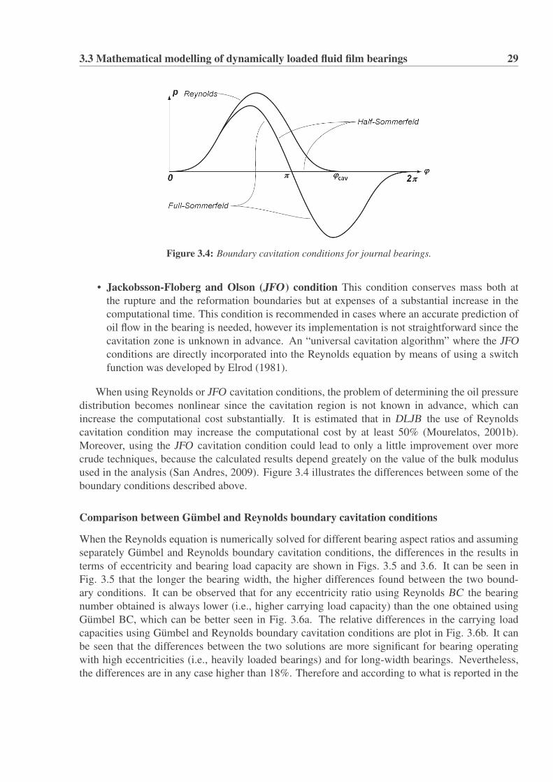
3.3 Mathematical modelling of dynamically loaded fluid film bearings 29
Figure 3.4: Boundary cavitation conditions for journal bearings.
• Jackobsson-Floberg and Olson (JFO ) condition This condition conserves mass both atthe rupture and the reformation boundaries but at expenses of a substantial increase in thecomputational time. This condition is recommended in cases where an accurate prediction ofoil flow in the bearing is needed, however its implementation is not straightforward since thecavitation zone is unknown in advance. An “universal cavitation algorithm” where the JFOconditions are directly incorporated into the Reynolds equation by means of using a switchfunction was developed by Elrod (1981).
When using Reynolds or JFO cavitation conditions, the problem of determining the oil pressuredistribution becomes nonlinear since the cavitation region is not known in advance, which canincrease the computational cost substantially. It is estimated that in DLJB the use of Reynoldscavitation condition may increase the computational cost by at least 50% (Mourelatos, 2001b).Moreover, using the JFO cavitation condition could lead to only a little improvement over morecrude techniques, because the calculated results depend greately on the value of the bulk modulusused in the analysis (San Andres, 2009). Figure 3.4 illustrates the differences between some of theboundary conditions described above.
Comparison between Gumbel and Reynolds boundary cavitation conditions
When the Reynolds equation is numerically solved for different bearing aspect ratios and assumingseparately Gumbel and Reynolds boundary cavitation conditions, the differences in the results interms of eccentricity and bearing load capacity are shown in Figs. 3.5 and 3.6. It can be seen inFig. 3.5 that the longer the bearing width, the higher differences found between the two bound-ary conditions. It can be observed that for any eccentricity ratio using Reynolds BC the bearingnumber obtained is always lower (i.e., higher carrying load capacity) than the one obtained usingGumbel BC, which can be better seen in Fig. 3.6a. The relative differences in the carrying loadcapacities using Gumbel and Reynolds boundary cavitation conditions are plot in Fig. 3.6b. It canbe seen that the differences between the two solutions are more significant for bearing operatingwith high eccentricities (i.e., heavily loaded bearings) and for long-width bearings. Nevertheless,the differences are in any case higher than 18%. Therefore and according to what is reported in the

30 Chapter 3. Dynamically Loaded Journal Bearings - DLJBs
literature (Mourelatos, 2001b), there are several cases where Gumbel conditions can be used with-out significant lack of accuracy, as in SJB and not very heavily loaded journal bearings. In othercases, a decision has to be made based on a trade-off between the computational cost involved andthe required level of accuracy of the results.
Sommerfeld Number, S
Eccentricityratio,ε
Gumbel BC
Reynolds BC
λ = 0.25
λ = 0.5λ = 1
λ = 2
10−3 10−2 10−1 100 101 102 1030
0.2
0.4
0.6
0.8
1
Figure 3.5: Effect of using Gumbel and Reynolds boundary conditions - Eccentricity ratio vs Sommerfeld
number.
Eccentricity ratio, ε
BearingLoad,Fb[N
]
(a) Gumbel BC Reynolds BC
Eccentricity ratio, ε
%
(b) λ = 2
λ = 1
λ = 0.5λ = 0.25
λ = 0.25λ = 0.5
λ = 1λ = 2
0 0.1 0.2 0.3 0.4 0.5 0.6 0.7 0.8 0.9 1
0 0.1 0.2 0.3 0.4 0.5 0.6 0.7 0.8 0.9 1
0
5
10
15
10−2
100
102
104
Figure 3.6: Effect of using Gumbel and Reynolds boundary conditions - (a) Bearing load capacity vs eccen-
tricity ratio; (b) Differences in bearing load capacity.

Chapter 4
From Hybrid to Controllable Lubrication
4.1 Actively lubricated bearings
During the last twenty years, the combination of tribology, control techniques and informatics hasenabled the development of active lubricated bearings, which are not only able to support the rotat-ing shaf but to deal with multi-objective functions (e.g., increasing of the film thickness, reductionof friction, enlarging of stability margins, modification of stiffness and damping parameters andreduction of cross-coupling effects). A recent literature review of theoretical and experimentalachievements in the development of active tribological systems is given in (Santos, 2009). Amongthe industrial applications using active lubrication, is the case of industrial gas compressors. Inthat case, lateral vibrations and rotor-bearing stability were improved by using active lubricated tilt-ing pad journal bearings (Santos et al., 2004), and multirecess active journal bearings with activepockets (Santos and Watanabe, 2006).
The bearing considered in this study is a hole-entry type bearing with orifices disposed circum-ferentially along two rows, as shown in Fig. 4.1. In these type of bearings, active lubrication isachieved by injecting oil at controllable pressures Pin j(t), through radial orifices. From the pointof view of active lubrication, and specifically considering the case of a dynamically loaded journalbearing, Pin j must be dynamically controlled. Although in this work several control pressure rulesare proposed based on the periodic behaviour of bearing loads in reciprocating machines, the studyhas been more focused on the evaluation of bearing performance parameters for different hybridbearing configurations, than in the design of the control system itself.
4.1.1 The modified Reynolds equation for active lubrication
Assuming an isoviscous, Newtonian, incompressible fluid operating in laminar regime, the govern-ing equation for the hydrodynamic pressure distribution of an active lubricated journal bearing canbe obtained from the Navier Stokes equation and the continuity equation by accommodating in theassumed boundary conditions the velocity profile of the oil injection, which is described in detail in(Santos and Russo, 1998; Santos et al., 2001). Thus, the pressure distribution for a journal bearingwith radial oil injection through orifices located at (ϕi,zi) along the bearing surface, is governed byEq. (4.1).
31

32 Chapter 4. From Hybrid to Controllable Lubrication
∂∂ϕ
(h3
rb2
∂ p
∂ϕ
)+
∂∂ z
(h3 ∂ p
∂ z
)− 3
lo
s
∑i=1
�i(ϕ,z) · p
= 12μcb
[ε cosϕ + ε sinϕ(φ − Ω
2)
]− 3
lo
s
∑i=1
�i(ϕ,z) · Pin j(t)
(4.1)
where: �i(ϕ,z) =
{d2
o4 −R2 if R2 ≤ d2
o/40 if R2 ≥ d2
o/4; and R2 = rb
2(ϕ −ϕi)2 +(z− zi)
2.
The function �i(ϕ,z) is used to describe mathematically the problem and is physically relatedto the position of the orifices. In other words, this function will be different than zero inside theorifices region and will be zero elsewhere. On the other hand, Pin j(t) gives the injection pressure ateach orifice in function of time. It can be noted that when the radial oil injection is not operating(i.e., Pin j = 0 and �i(ϕ,z) = 0), Eq. (4.1) translates into the conventional Reynolds equation forhydrodynamic lubrication, given by Eq. (3.4). Equation (4.1) can be numerically solved for thepressure distribution (p(ϕ,z)) using finite differences, provided that the normal squeeze velocity (ε)and the rotational velocities (φ and Ω) are known from the dynamics of the mechanical system, asshown in section 4.1.2. It is worth noting that for the developing of the modified Reynolds equationfor active lubrication, inertia and compressibility effects were disregarded. The fluid inertia effectswere neglected considering that at not very high journal rotational speeds, the effects of viscousforces are more important than inertia effects. On the other hand, compressibility effects havenot been included into the equations, considering that their influence on the fluid film pressuredistribution and minimum fluid film thickness can be disregarded compared to the squeezing andwedge effects on the fluid film, when maximum film pressures are not considerably high (e.g.,pmax ≤ 12 MPa), as shown in the cases of study included in chapter 6.
Figure 4.1: Hole-entry type journal bearing.

4.1 Actively lubricated bearings 33
4.1.2 Numerical solution of the modified Reynolds equation for active lubri-cation
A FD scheme with the assumption of isothermal conditions was adopted. In order to be able torefine the mesh over the area where the orifices for oil injection are located, and consequently toobtain a better estimation of the film pressures and minimum fluid film thicknesses, a non-uniformgrid has been use to discretize the bearing domain, as shown in Fig. 4.2. Similarly to the FD schemeoutlined in section 3.3.2, but for a non-uniform discretization, using a central difference scheme,the first and second order derivatives can be written as:
∂ p
∂ϕ
∣∣∣∣m,n
=pm+1,n − pm−1,n
Δϕm−1 +Δϕm(4.2)
∂ 2 p
∂ϕ2
∣∣∣∣m,n
=2
Δϕm−1 +Δϕm
(pm+1,n − pm,n
Δϕm− pm,n − pm−1,n
Δϕm−1
)(4.3)
Assuming that the bearing is well aligned (i.e., ∂h/∂ z = 0) and the viscosity of the fluid filmkeeps constant, the modified Reynolds equation in finite differences is given by equation (4.4).
Δm,n pm−1,n +Λm,n pm+1,n +♦m,n pm,n +∇m,n pm,n−1 +�m,n pm,n+1
= 12μcbrb2[
ε cosϕm,n + ε sinϕm,n(φ − Ω2)
]− 3r2
b
lo
s
∑i=1
�im,nPin j
(4.4)
where:
Δm,n =1
Δϕm +Δϕm−1
[−3h2
m,n∂h
∂ϕ
∣∣∣∣m,n
+2h3
m,n
Δϕm−1
];
Λm,n =1
Δϕm +Δϕm−1
[3h2
m,n∂h
∂ϕ
∣∣∣∣m,n
+2h3
m,n
Δϕm
];
♦m,n = −2h3m,n
[1
Δϕm +Δϕm−1
(1
Δϕm+
1Δϕm−1
)
+r2
b
Δzn +Δzn−1
(1
Δzn+
1Δzn−1
)]− 3r2
b
lo
s
∑i=1
�im,n · pm,n ;
∇m,n =2h3
m,nr2b
Δzn−1
1Δzn +Δzn−1
; �m,n =2h3
m,nr2b
Δzn
1Δzn +Δzn−1
.
Assuming the Gumbel boundary conditions, and applying atmospheric pressures at the edges ofthe bearing, Eq. (4.4) can be solved by an iterative method such as the well known SOR (successiveover relaxation) method, or by a factorization method, such as Cholesky or LU methods. In thiswork, the LU method was adopted. The modified Reynolds equation (4.1) can be solved for eachtime step if the oil injection pressures through the orifices (Pin j) are known as a function of theinstantaneous crank angle.

34 Chapter 4. From Hybrid to Controllable Lubrication
Figure 4.2: Non-uniform finite difference mesh.
In order to be able to control the oil injection pressures through the bearing orifices, differentalternatives could be considered. Among them: mechanical cam systems, hydraulic servovalves(Santos et al., 2004; Santos and Russo, 1998) and piezoelectric nozzles (Horikawa et al., 1992;Mizumoto et al., 1996). The use of a piezo-actuated injection system and a mechanical unit injectorwere considered in this work. Some insights into their modelling are given in the next section.
4.1.3 Hybrid bearing configuration
Considering the geometric bearing configuration shown in Fig. 4.1, active or controllable lubricationis achieved by radially injecting oil at pressures that may be controlled in function of the instanta-neous crank angular position. In order to advantageously modify the hydrodynamic bearing fluidfilm by applying controllable radial oil injection (i.e., hybrid lubrication), a suitable distribution ofthe injection orifices on the bearing surface, and appropriate control rules for the oil injection pres-sures have to be determined, which has been also investigated in (Estupinan and Santos, 2009c,a).Thus, important sources of information when attempting to configure and/or optimize oil injectionare: the bearing acting loads, the curves of combustion forces inside the cylinders and the behaviourof bearing parameters when bearings operate under conventional lubrication conditions. In thestudy of Estupinan and Santos (2009c,a) appropriate locations for the injection orifices and conve-nient rules for changing the oil injection pressures (as a function of the instantaneous crankshaftangle), were found. However, details related to the oil injection system were not discussed.
The performance of a hybrid journal bearing depends on several geometric parameters, such as,diameter of the injection orifices, position of the orifices, bearing aspect ratio (λ ), and axial landwidth ratio (ab). Therefore, depending on the load and speed working conditions, several types ofconfigurations are possible (Stout and Rowe, 1974; Rowe et al., 1982). In order to optimize geomet-rically the design of hybrid journal bearings under different external load conditions, several studieshave been carried out for specific cases, mainly related to stationary loaded conditions (Sharmaet al., 1999; Jadon and Singh, 2007). Particularly, it was shown by Rowe et al. (1982), that hole-entry bearings with holes disposed circumferentially along two rows may offer advantages overother configurations.

4.2 Schemes for applying radial oil injection 35
Figure 4.3: Hybrid bearing geometry.
4.2 Schemes for applying radial oil injectionThis section presents a theoretical study that describes two different schemes for the oil injectionsystem in actively or controllable lubricated DLJBs, using controllable radial oil injection to modifythe conventional hydrodynamic lubrication. Figure 4.3 shows another view of the hole-entry typebearing considered in this study for applying controllable radial oil injection. The main equationsthat govern the dynamics of the injection for a piezo-actuated oil injector and a mechanical-actuatedoil injector are presented in this section. In chapter 5 it will be shown how the dynamics of the oilinjection system is coupled to the dynamics of the bearing fluid film through equations, and how theglobal system is numerically solved. Later in chapter 6 numerical results for the main bearing of asingle-cylinder ICE, using a piezo-actuated injection system will be presented.
In the following, two alternatives for applying the oil injection are presented: a) a piezo-actuatedinjection system; and b) a mechanical unit injection system, as schematically illustrated in Figs. 4.4and 4.8. The proposed designs for these two types of oil injectors are based on similar workingprinciples of the injectors used in fuel injection systems in vehicles. However, notice that importantdifferences in the fluid properties and level of injection pressures required for active lubrication,must be considered in the modelling. The main focus of the mathematical modelling of the oilinjection systems was mainly put on the derivation of the equations that govern the dynamics of theinjectors and their coupling to the dynamics of the fluid film bearings.
4.2.1 Piezoelectric injection systemPiezoceramic actuators has become an area of increased interest in the past fifteen years, due theseveral advantages they present when compared to mechanical and electro-mechanical actuators(Ulbrich, 1994). Among relevant work covering reviews of state-of-the-art actuators, and includingcomparison between them in terms of electrical and mechanical properties, and potential applica-tions, are the studies of Near (1996); Prechtl and Hall (1999); Taylor and Washington (2002). Inthese studies was shown that piezoelectric actuators generally present a more compact design and

36 Chapter 4. From Hybrid to Controllable Lubrication
faster response when compared to other type of actuators.The piezo-actuated oil injection system described in this section is schematically shown in
Fig. 4.4. In this type of injector, the injection is controlled by the activation of a piezoelectricactuator. If the piezoelectric stack (pz) is activated by a voltage signal, the control valve (cv) opens,which results in a pressure drop in the control chamber (cc), and subsequently the opening of theinjection nozzle due to the lift of the needle valve (nv), starting the injection. When the feeding volt-age applied to the piezoelectric stack is deactivated, the control valve returns to the closed position,the servopiston and needle valve move downwards and consequently the injection ends. Severalstudies for the modelling of similar type of injectors, but for diesel fuel injection systems are foundin the literature (Lee et al., 2002; Lino et al., 2007; Chung et al., 2008). The mathematical modellingof the piezo-actuated injector presented in this case, is based on the same methodology describedby Chung et al. (2008). The main governing equations for the hydraulic, mechanical and electricalsubsystems will be presented next.
Figure 4.4: Schematics of a piezo-actuated injector.

4.2 Schemes for applying radial oil injection 37
For the simplicity of the modelling, the following main assumptions are made:
• oil supply pressure (Ps) is constant, i.e., the dynamics of the oil supply pump are not included.
• solid parts of injector are rigid, i.e., elastic deformations of solid parts due to pressure changeare neglected.
• internal leakages are neglected.
The main equations for the modelling of the piezoelectric actuator and the hydraulic and me-chanical subsystems of the injector are presented in the following section.
Modelling of the piezoelectric stack:
The material strain and the electrical displacement exhibited by a piezoelectric stack are both lin-early affected by the mechanical stress and electrical field to which the ceramic is subjected, asstated by the linear constitutive equations for piezoelectric materials (ANSI/IEEE, 1987). In thecase of defining the constitutive equations for piezostacks, it is typical that poling and loading di-rections to be defined as the 3,3 directions respectively, as shown in Fig. 4.5a. The linear constitutiveequations for piezoelectric materials are defined as:
S3(t) = sE33T3(t)+d33E3(t) (4.5)
D3(t) = d33T3(t)+ εT33E3(t) (4.6)
where S3(t) is the strain; s33 is the elastic compliance [m2/N]; T3(t) is the stress; d33 is the piezo-electric coupling coefficient (or piezo electric charge constant) [C/N]; E3(t) is the electric field= v(t)/d; D3(t) is the electric displacement = Q3(t)/Apz; ε33 is the dielectric permittivity [F/m].Thus, Eq. (4.5) defines the mechanical response of the material while Eq. (4.6) defines the electricalresponse.
(a) (b)
Figure 4.5: (a) Schematic configuration of a piezostack (Feenstra et al., 2008); (b) Mechanical design of a
comercial stack actuator.

38 Chapter 4. From Hybrid to Controllable Lubrication
Considering that a stack actuator has several layers of piezoelectric material, the number oflayers (Npz), with each layer of an area of Apz, and thickness dpz, the resultant piezo-stack force(Fpz) and electric charge can be derived from the constitutive equations for piezoelectric materials:
Fpz(t) =−k33xpz(t)+ k33d33Npzvpz(t) (4.7)
Qpz(t) = k33d33xpz(t)+ ε33NpzE−1pz vpz(t) (4.8)
where xpz(t) is the total displacement of the piezo-stack; k33 is the elastic stiffness of the piezo-stack;d33 is the piezoelectric coupling coefficient; vpz is the feeding voltage; Epz is the elastic modulus ofthe piezo-stack; and ε33 is the dielectric permittivity. If the hysteresis is assumed to be negligible,the free expansion of an unloaded piezoelectric stack actuator may be expressed by (Fuller et al.,1996):
ΔLpz(t) = d33Npzvpz(t) (4.9)
Modelling of hydraulic subsystems:
The hydraulic subsystems are considered as containers of unknown pressure, where the cross-sectional area is great compared with the inlet and outlet ducts of the system. Considering onlyelasticity of the concentrated volume but not inertia effects, an equal pressure inside the controlvolume can be assumed. Considering compressibility of the fluid, expressed by the bulk modulusof elasticity, the pressure change in each one of the control volumes vi of the hydraulic subsystems(i.e., control valve (cv), control chamber (cc) and needle injector valve (nv)), can be solved by meansof Eq. (4.10), derived from the definition of bulk modulus of elasticity (Fox et al., 2004):
dP
dt=−β
V
dV
dt(4.10)
where β is the bulk modulus of elasticity; V is the instantaneous volume of the fluid; dV/dt takesinto account the intake and outtake flows, Qin and Qout , and the volume change due to the motionof mechanical parts. The above equation yields:
dPvi
dt=−βvi
Vvi
(dVvi
dt−Qin
vi+Qout
vi
)(4.11)
where for each control volume, Vviis the instantaneous volume of the fluid; dVvi
/dt accounts for thevolume change due to the motion of mechanical parts. The bulk modulus can be related to the fluidpressure by (Hountalas and Kouremenos, 1998):
βvi= 1.2×10⁹
[1+0.6
Pvi×10−5
600
](4.12)
The intake and outtake flows through each control volume Qin and Qout , can be calculated by ap-plying the energy conservation law:
Q = sgn(ΔP) ·Cd ·Ao ·√
2ρ|ΔP| (4.13)

4.2 Schemes for applying radial oil injection 39
where for each control volume at the inlet and outlet section, respectively: Cd is a discharge coeffi-cient; Ao is the orifice section; ΔP is the oil pressure difference across the section Ao; and ρ is the oildensity. The discharge coefficient Cd accounts for the flow losses through orifices and it is usuallyobtained experimentally. In the literature there is a wide spread of values for discharge coefficients,however, for short and sharp-edged orifices a value of Cd = 0.6 is commonly assumed for numericalsimulations (Merritt, 1967). Applying Eqs. (4.11) and (4.13) to the hydraulic subsystems of thepiezo-actuated injector (see Fig. 4.4), one obtains:
Control valve (cv):
Pcv =−βcv
Vcv
⎛⎜⎜⎜⎜⎝Vcv − sgn(Pcc −Pcv)C
indcv
Ainocv
√2ρ|Pcc −Pcv|︸ ︷︷ ︸
Qincv
+sgn(Pcv −Pt)Coutdcv
Aoutocv
√2ρ|Pcv −Pt |︸ ︷︷ ︸
Qoutcv
⎞⎟⎟⎟⎟⎠
(4.14)Control chamber (cc):
Pcc =−βcc
Vcc
⎛⎜⎜⎜⎜⎝Vcc − sgn(Ps −Pcc)C
indcc
Ainocc
√2ρ|Ps −Pcc|︸ ︷︷ ︸
Qincc
+sgn(Pcc −Pcv)Coutdcc
Aoutocc
√2ρ|Pcc −Pcv|︸ ︷︷ ︸
Qoutcc
⎞⎟⎟⎟⎟⎠
(4.15)Needle valve (nv):
Pin j =−βnv
Vnv
⎛⎜⎜⎜⎜⎝Vnv − sgn(Ps −Pin j)C
indnv
Ainonv
√2ρ|Ps −Pin j|︸ ︷︷ ︸
Qinnv
+sgn(Pin j − Pjb)Coutdnv
Aoutonv
√2ρ|Pin j − Pjb|︸ ︷︷ ︸
Qoutnv ⇔Qin j
⎞⎟⎟⎟⎟⎠
(4.16)where Pcv is the pressure in the control valve; Pcc is the pressure in the control chamber; Ps is thesupply pressure; Pt is the return pressure; and Pin j is the injection pressure.
Assuming incompressible flow and no pipeline deformations, the oil flow passing through thebearing orifice area Aout
onvcan be calculated by integrating the injection velocity profile:
Qin j =∫
AVin jdA (4.17)
where the injection velocity profile for each ith orifice, can be written as a function of the differencebetween the journal pressure Pjbi
(ϕ,z, t) and the injection pressure Pin ji(t), assuming a fully devel-oped laminar flow in an axisymmetric pipe and a linear variation of the injection pressure along theorifice (Santos and Russo, 1998):
Vin j(ϕ,z, t) =−�i(ϕ,z)4μlo
(Pin j(t)− Pjb(ϕ ,z, t)) (4.18)

40 Chapter 4. From Hybrid to Controllable Lubrication
Figure 4.6: Needle tip geometry.
In Eq. (4.18), Pjb corresponds to the film pressure computed at the sleeve side of the orifice,obtained from the solution of the modified Reynolds equation (Eq. (4.1)). In other words, for eachone of the ith oil injection orifices, Pjbi
would be equal to p evaluated at the coordinates Θoi,abi
(seeFig. 4.1). Since the value of Pjb depends on the dynamics of the journal bearing fluid film, its valuemust be updated for each time step in Eq. (4.16).
The total oil flow passing through all the s orifices can be calculated as:
Qin j(t) =−s
∑i=1
∫Vin ji(t).dAi (4.19)
It is worth to notice that in Eq. (4.16) the cross section area of the inlet flow (Ainonv
) is not constantand it can be written as a function of the displacement of the needle of the injector (xnv), as follows:
Ainonv
=π4(dns +din)
√(dns −din)2 + x2
nv (4.20)
where dns is the diameter of the needle seat, and din is a variable given by: din = dns−2xnv cosθns sinθns;θns is the angle of the tip of the needle injector, as illustrated in Fig. 4.6.
Modelling of mechanical subsystems:
In order to model the main mechanical parts of the piezoelectric injector, they are grouped in twomechanical subsystems s1 and s2, and described by sdof systems, as schematically seen in Fig. 4.7The first mechanical subsystem consists of the push rod, valve piston, control valve and piezoelectricstack, and it is dynamically described by Eq. (4.21). The second subsystem includes the controlpiston and the needle valve, and it is described by the Eq. (4.22).
ms1xcv = Fpz − ks1xcv − cs1xcv −AcvPcv (4.21)
ms2xnv =−ks2xnv − cs2xnv −ApPcc +(Anv −Ans)Ps (4.22)
where ms1 is given by the equivalent mass of the control valve cluster and the piezoelectric stack;ms2 is given by the total mass of the needle valve and control piston; cs1 is the viscous frictioncoefficient of the valve piston; ks1 is the combined stiffness of the push rod and valve springs; cs2is the viscous friction coefficient of the needle injector; ks2 is the servo piston spring constant; Anv,Ans, Ap, Acv are the sectional area of the needle valve, needle valve seat, servo piston and controlvalve respectively, as shown in Fig. 4.4.

4.2 Schemes for applying radial oil injection 41
(a) (b)
Figure 4.7: (a) Equivalent mechanical subsystem ms1: piezostack; pushrod and control valve; (b) equivalent
mechanical subsystem ms2: valve piston and needle valve.
Mathematical model in state space representation
All the equations that describe the mathematical model of the piezo-actuated injector can be rewrit-ten in state space form as
xxx(t) = f (t,xxx(t),vvvpz(t))
where xxx = [xpz xpz xnv xnv Pcv Pcc Pin j]T ; and the piezo-stack driving signals are the inputs: vvvpz(t) =
[vpz(t) vpz(t)]T . As a result, the state space representation is given by:⎧⎪⎪⎪⎪⎪⎪⎪⎪⎪⎪⎪⎪⎪⎪⎪⎨
⎪⎪⎪⎪⎪⎪⎪⎪⎪⎪⎪⎪⎪⎪⎪⎩
xpz
xpz
xnv
xnv
Pcv
Pcc
Pin j
⎫⎪⎪⎪⎪⎪⎪⎪⎪⎪⎪⎪⎪⎪⎪⎪⎬⎪⎪⎪⎪⎪⎪⎪⎪⎪⎪⎪⎪⎪⎪⎪⎭
⇔
⎧⎪⎪⎪⎪⎪⎪⎪⎪⎪⎪⎪⎪⎪⎪⎪⎨⎪⎪⎪⎪⎪⎪⎪⎪⎪⎪⎪⎪⎪⎪⎪⎩
x1
x2
x3
x4
x5
x6
x7
⎫⎪⎪⎪⎪⎪⎪⎪⎪⎪⎪⎪⎪⎪⎪⎪⎬⎪⎪⎪⎪⎪⎪⎪⎪⎪⎪⎪⎪⎪⎪⎪⎭
=
⎧⎪⎪⎪⎪⎪⎪⎪⎪⎪⎪⎪⎪⎪⎪⎪⎨⎪⎪⎪⎪⎪⎪⎪⎪⎪⎪⎪⎪⎪⎪⎪⎩
x2
[−k33x1 + k33d33Npzvpz − ks1x1 − cs1x2 −Acvx5]/ms1
x4
[−ks2x3 − cs2x4 −Apx6 +(Anv −Ans)Ps]/ms2
−βcv(x5)Vcv
[Acvx2 −Qin
cv(x5,x6)+Qoutcv (x5)
]−βcc(x6)
Vcc(x3)
[Accx4 −Qin
cc(x6)+Qoutcc (x5,x6)
]−βiv(x7)
Viv
[Viv(x3)−Qin
iv(x7)+ Qin j(x7, Pjb)]
⎫⎪⎪⎪⎪⎪⎪⎪⎪⎪⎪⎪⎪⎪⎪⎪⎬⎪⎪⎪⎪⎪⎪⎪⎪⎪⎪⎪⎪⎪⎪⎪⎭
(4.23)
A simplified model of piezo-injector
The modelling of the injector can be simplified by considering it as a control volume without con-sidering the dynamics of the piezo-stack and the control chambers. It can be also assumed thatthe volume of the injector chamber remains constant and that the injection section area switchesbetween zero and its maximum, neglecting opening and closing transients of the injector. Thus, thegoverning pressure for the injection can be rewritten as:
Pin j =−βiv
Viv
(−sgn(Ps −Pin j)STC∗
dnv
√|Ps −Pin j|+ Qin j
)(4.24)

42 Chapter 4. From Hybrid to Controllable Lubrication
where ST is a square signal equal to 1 during injections and zero otherwise; and C∗dnv
=Cindnv
Amaxonv
√2/ρ .
The equations of the dynamics of the injector and the system of equations that describes thedynamics of journal bearing and reciprocating mechanism have to be simultaneously solved, sincethe oil injection pressures (Pin j) are influenced by the hydrodynamic pressure of the fluid film at thebearing side of the orifices (Pjb), as seen in Eq. (4.16). At the same time, the updated values of Pin j
have to be introduced into Eq. (4.1) for each time step.
4.2.2 Mechanical injection system
In the mechanical injector described here, the injection is basically controlled by an inline cam-pump system, where the design of the cam profile determines the oil injection events. An schematicdiagram is shown in Fig. 4.8. The governing equations for the dynamics of the hydraulic subsystems(i.e., needle injector valve and pump) can be deducted from Eqs. (4.11) and (4.13). In this case, thedynamics of the pump has to be included in the model since the oil flows and pressures in the controlvolumes directly depend on the performance of the pump. To simplify the modelling of the injection,the connecting pipe between delivery valve and accumulator injector chamber is considered short,neglecting loss factors and pressure variations related to pressure waves propagation. Moreoverthe modelling of the delivery valve is simplified by considering it as a check valve and assuringthat only flow from the pump to the accumulator chamber takes place. Previous studies relatedto the modelling of fuel injectors have shown that by neglecting the effects of the valve motionthe introduced error is small compared to more sophisticated models (Hountalas and Kouremenos,1998). With these simplifications, the governing equation for the pressure change in the hydraulicsubsystems of the mechanical oil injection system can be written as
Cylinder pump (cp):
Pcp =−βcp
Vcp
⎛⎜⎜⎜⎜⎜⎝ ˙Vcp − sgn(Pcp −Ps)C
indcp
Ainocp
√2ρ|Pcp −Ps|︸ ︷︷ ︸
Qincp
+sgn(Pdv −Pcp)Coutdcp
Aoutocp
√2ρ|Pdv −Pcp|︸ ︷︷ ︸
Qoutcp ⇔Qin
dv
⎞⎟⎟⎟⎟⎟⎠
(4.25)Delivery valve (dv):
Pdv =−βdv
Vdv
(−Qindv +Qout
dv
)(4.26)
Accumulator chamber (ac):
Pac =−βac
Vac
⎛⎜⎜⎜⎜⎝−sgn(Pac −Pdv)C
indac
Ainoac
√2ρ|Pac −Pdv|︸ ︷︷ ︸
Qinac⇔Qout
dv
+Qoutac︸︷︷︸
Qinnv
⎞⎟⎟⎟⎟⎠ (4.27)
Needle valve (nv):

4.2 Schemes for applying radial oil injection 43
Figure 4.8: Schematics of a mechanical unit injector.
Pin j =−βnv
Vnv
⎛⎜⎜⎜⎜⎝Vnv − sgn(Pac −Pin j)C
indnv
Ainonv
√2ρ|Pac −Pin j|︸ ︷︷ ︸
Qinnv
+sgn(Pin j − Pjb)Coutdnv
Aoutonv
√2ρ|Pin j − Pjb|︸ ︷︷ ︸
Qoutnv ⇔Qin j
⎞⎟⎟⎟⎟⎠
(4.28)where
Qindv = Qout
cp , if Pcp > Pdv ; otherwise Qindv = 0
Qoutdv = Qin
ac , if Pdv > Popdv ; otherwise Qout
dv = 0
where Pcp is the pressure inside the cylinder of the pump; Pdv is the pressure in the delivery valvechamber; Pac is the pressure in the accumulator chamber; Pin j is the injection pressure; and P
opdv is
the opening pressure of the delivery valve.The change of volume due to piston motion can be calculated by knowing the position of the
plunger with respect to the camshaft angle - zp(θcs), which can be obtained by linear interpolationof the cam profile. Hence, the instantaneous pump volume and the rate of change of pump volume

44 Chapter 4. From Hybrid to Controllable Lubrication
as a function of piston motion are given by:
Vcp =V 0cp −Acp · zp(θcs) (4.29)
Vcp = Acp · zp = Acp ·Ωcs · dzp
dθcs(4.30)
where Acp is the cylinder bore; zp is the piston instantaneous axial displacement; V 0cp is the cylinder
total volume; and Ωcs is the camshaft speed.Assuming a SDOF system, the displacement of the injector valve (needle injector) is calculated
byms3xnv =−ks3(xnv + xpl)− cs3xnv +(Anv −Ans)Pac (4.31)
where xpl is the preload of the needle valve spring; ks3 and cs3 are the stiffness of the spring anddamping (friction) coefficient, respectively; and ms3 is the equivalent mass for the injector valve.
Mathematical model in state space representation
The equations that describe the mathematical model of the mechanical unit injector can be rewrittenin state space form as
xxx(t) = f (t,xxx(t),uuucs(t))
where xxx = [xnv xnv Pcp Pdv Pac Pin j]T ; and the movement of the plunger in the pump, which depends
on the camshaft profile and rotational velocity are the inputs: uuucs(t) = [zp(t) zp(t)]T , where zp(t) =
Ωcs(dzp/dθcs). As a result, the state space representation is given by:⎧⎪⎪⎪⎪⎪⎪⎪⎪⎪⎪⎪⎪⎨⎪⎪⎪⎪⎪⎪⎪⎪⎪⎪⎪⎪⎩
xnv
xnv
Pcp
Pdv
Pac
Pin j
⎫⎪⎪⎪⎪⎪⎪⎪⎪⎪⎪⎪⎪⎬⎪⎪⎪⎪⎪⎪⎪⎪⎪⎪⎪⎪⎭
⇔
⎧⎪⎪⎪⎪⎪⎪⎪⎪⎪⎪⎪⎪⎨⎪⎪⎪⎪⎪⎪⎪⎪⎪⎪⎪⎪⎩
x1
x2
x3
x4
x5
x6
⎫⎪⎪⎪⎪⎪⎪⎪⎪⎪⎪⎪⎪⎬⎪⎪⎪⎪⎪⎪⎪⎪⎪⎪⎪⎪⎭
=
⎧⎪⎪⎪⎪⎪⎪⎪⎪⎪⎪⎪⎪⎨⎪⎪⎪⎪⎪⎪⎪⎪⎪⎪⎪⎪⎩
x2[−ks3(x1 + xpl)− cs3x2 +(Anv −Ans)x5]/ms3
−βcp(x3)Vcp(zp)
[Acpzp −Qin
cp(x3)+Qoutcp (x3,x4)
]−βdv(x4)
Vdv
[−Qindv(x3,x4)+Qout
dv (x4,x5)]
−βac(x5)Vac
[−Qinac(x4,x5)+Qout
ac (x5,x6)]
−βnv(x6)Vnv(x1)
[Vnv(x2)−Qin
nv(x5,x6)+ Qin j(x6, Pjb)]
⎫⎪⎪⎪⎪⎪⎪⎪⎪⎪⎪⎪⎪⎬⎪⎪⎪⎪⎪⎪⎪⎪⎪⎪⎪⎪⎭
(4.32)
A simplified model of the mechanical unit injector
In order to simplify the modelling of the mechanical injector, and to facilitate afterwards the de-sign of the controller, the model can be reduced by neglecting the dynamics of delivery valve andthe injector, assuming that the outflow section areas switches between zero and its maximum, thusneglecting opening and closing transients. Additional assumptions consider the flow between thepump and the delivery equal to the flow between the delivery valve and the accumulator cham-ber; and the flow between the accumulator chamber and the injector equal to the flow between theinjector and the journal bearing. With these simplifications, the governing equations become:

4.3 Summary 45
Pcp =−βcp
Vcp
⎛⎜⎜⎜⎜⎜⎝ ˙Vcp − sgn(Pcp −Ps)C
indcp
Ainocp
√2ρ|Pcp −Ps|︸ ︷︷ ︸
Qincp
+sgn(Pac −Pcp)Coutddv
Aoutodv
√2ρ|Pac −Pcp|︸ ︷︷ ︸
Qoutcp ⇔Qin
ac
⎞⎟⎟⎟⎟⎟⎠
(4.33)
Pac =−βac
Vac
⎛⎜⎜⎜⎜⎜⎝−sgn(Pac −Pcp)C
outddv
Aoutodv
√2ρ|Pac −Pcp|︸ ︷︷ ︸
Qinac⇔Qout
cp
+sgn(Pac − Pjb)C∗dnv
ST
√|Pac − Pjp|︸ ︷︷ ︸
Qoutac ⇔Qin j
⎞⎟⎟⎟⎟⎟⎠
(4.34)
where ST is a square signal equal to 1 during injections and zero otherwise; and C∗dnv
=Cindnv
Amaxonv
√2/ρ .
4.3 SummaryTwo approaches for applying active lubrication to DLJBs were described in this chapter. Hydro-static lubrication is modified by injecting oil at controllable pressures, through orifices circumferen-tially located around the bearing surface. The modified Reynolds equation for active lubrication andfor DLJBs was presented and discretized in order to be solved using a FD scheme. The main equa-tions that govern the dynamics of the injection for a piezo-actuated oil injector and a mechanical-actuated oil injector were presented. The next chapter describes how the injector dynamics (Eq. 4.23for the piezoelectric injector and Eq. 4.32 for the mechanical injector) is numerically coupled to thedynamics of the bearing fluid films, and to the representative MBD model of a reciprocating mech-anism (refer to Fig. 5.3). In chapter 6, the analysis of a main journal bearing of a reciprocating ICE,operating with controllable radial oil injection, and using a piezolectric injection system, will bediscussed.

46 Chapter 4. From Hybrid to Controllable Lubrication
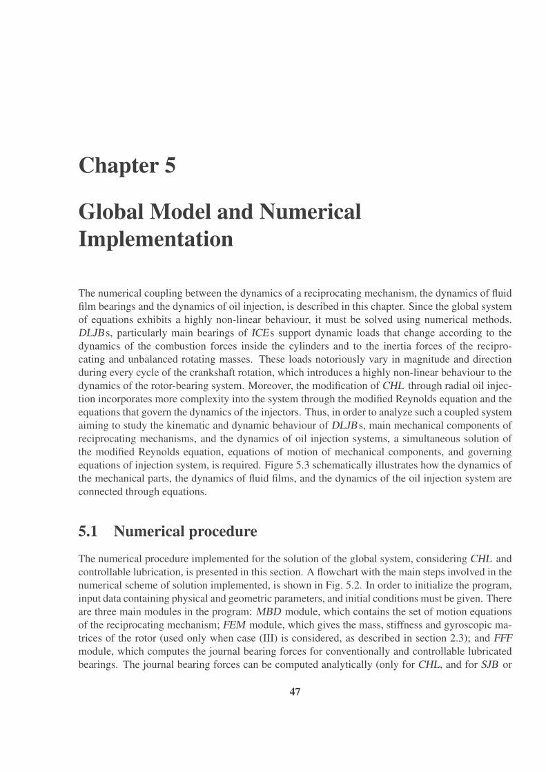
Chapter 5
Global Model and NumericalImplementation
The numerical coupling between the dynamics of a reciprocating mechanism, the dynamics of fluidfilm bearings and the dynamics of oil injection, is described in this chapter. Since the global systemof equations exhibits a highly non-linear behaviour, it must be solved using numerical methods.DLJBs, particularly main bearings of ICEs support dynamic loads that change according to thedynamics of the combustion forces inside the cylinders and to the inertia forces of the recipro-cating and unbalanced rotating masses. These loads notoriously vary in magnitude and directionduring every cycle of the crankshaft rotation, which introduces a highly non-linear behaviour to thedynamics of the rotor-bearing system. Moreover, the modification of CHL through radial oil injec-tion incorporates more complexity into the system through the modified Reynolds equation and theequations that govern the dynamics of the injectors. Thus, in order to analyze such a coupled systemaiming to study the kinematic and dynamic behaviour of DLJBs, main mechanical components ofreciprocating mechanisms, and the dynamics of oil injection systems, a simultaneous solution ofthe modified Reynolds equation, equations of motion of mechanical components, and governingequations of injection system, is required. Figure 5.3 schematically illustrates how the dynamics ofthe mechanical parts, the dynamics of fluid films, and the dynamics of the oil injection system areconnected through equations.
5.1 Numerical procedure
The numerical procedure implemented for the solution of the global system, considering CHL andcontrollable lubrication, is presented in this section. A flowchart with the main steps involved in thenumerical scheme of solution implemented, is shown in Fig. 5.2. In order to initialize the program,input data containing physical and geometric parameters, and initial conditions must be given. Thereare three main modules in the program: MBD module, which contains the set of motion equationsof the reciprocating mechanism; FEM module, which gives the mass, stiffness and gyroscopic ma-trices of the rotor (used only when case (III) is considered, as described in section 2.3); and FFFmodule, which computes the journal bearing forces for conventionally and controllable lubricatedbearings. The journal bearing forces can be computed analytically (only for CHL, and for SJB or
47

48 Chapter 5. Global Model and Numerical Implementation
LJB solutions), or numerically using a FD scheme. The main steps involved in the numerical solu-tion of the global system are summarized next.
5.1.1 Input data and starting valuesIn this part all of the geometric and physical parameters are given, i.e., geometric bearing con-figuration, dimensions of main mechanical parts, rotational speed of crankshaft, masses, inertias,preloads, etc. Suitable initial conditions must be given (i.e., displacements and initial velocities ofcomponents). In the cases where controllable lubrication is included, the geometric hybrid bearingconfiguration has to be defined, such as, distribution of orifices over the bearing surface and diam-eter of orifices, as well as, the rules for controlling oil injection pressures (Pin j(θc)). The geometricand physical characteristic of the injectors have to be included, if the system is going to be solvedconsidering the dynamics of the injection system.
5.1.2 Pre-processingBased on the input data, starting values given to the program, and the case of analysis considered,the system of equations for the multibody dynamic model (MBD module) can be defined. It hasto be mentioned that MBD module is required for all cases, generating a different set of equationsfor each case, as shown in appendix A. If the flexibility of the rotor is to be considered, as in case(III), the matrices of the FEM formulation of the rotor are generated using FEM module. Duringthe preprocessing stage the discretization of Reynolds equation using a FD formulation takes place.In the cases where CHL is considered, the Reynolds equation is discretized using an uniform meshover the bearing surface, as presented in section 3.3.2. For the cases where controllable radial oilinjection is considered, a non-uniform mesh over the bearing surface is implemented, as the oneillustrated in Fig. 5.1, and described with equations in section 4.1.2.
45901351802252703153420
0.01
0.02
0.03
0.04
Θ [degrees]
z [m
]
Θo1
ab
Θ
Θo2
Z
Figure 5.1: Discretized bearing surface with a non-uniform mesh, size of m×n.

5.1 Numerical procedure 49
YesYes
ti+1 = ti + t
t < tfinal
< 1No
Cases II and IIIFFF Module
Journal bearing parameters for:- CHL and
- Controllable lubrication
Case IIIFEM Module
Rotor: [M],[K],[D]
Numerical solutionat t = ti
Numerical Integration:velocities and displacements.
Adjust tand go to start
Updating- Displacements
- Velocities
Computation ofJournal bearing forces
f (ti), f (ti)
Coupling of equations
Updating- Eccentricity,
- Attitude angle,p( , z, ti)
Input Data- Geometrical and
physical parameters
Plot Results
CHL- Setup of uniform FD mesh of RE
- Pinj=0
Controllable Lub.- Setup non-uniform FD mesh of RE
Define:- Hybrid bearing configuration
- Control pressure rules - Pinj( )
Cases I, II and IIIMBD Module
-Constrain equations- Motion equations
Injector Module:- Eqs. injector dynamics
Initial Conditions, t = t0- Displacements
-Velocities
Figure 5.2: Flowchart - overall solution scheme.

50 Chapter 5. Global Model and Numerical Implementation
Figu
re5.
3:C
oupli
ng
of
MB
Dm
odel
(case
II),
fluid
film
dyn
am
ics
(wit
hco
ntr
oll
able
lubri
cati
on),
and
dyn
am
ics
of
inje
ctor.

5.1 Numerical procedure 51
5.1.3 Calculation of the fluid film bearing forces
The numerical algorithm for solving Reynolds equation is implemented inside the FFF module.When CHL is considered, the fluid film forces can be computed using either analytical, or numer-ical solutions of Reynolds equation for DLJBs. The approximated analytical solutions for DLJBsoperating under CHL (given in Table 3.2) are recommended to be used only for SJB or LJB ap-proaches. In other cases numerical methods should be used for the solution of Reynolds equation.When a DLJB operates with active or controllable lubrication, the modified Reynolds equation foractive lubrication, presented in Eq. 4.1 has necessarily to be numerically solved. In this work theFD formulation described in section 4.1.2 was computationally implemented. Thus, the area overthe bearing surface was discretized using an uniform mesh (for the CHL case), or a non-uniformmesh (for the hybrid bearing case), as illustrated in Fig. 5.1, which enables to refine the area overthe oil injection orifices. The set of algebraic equations giving by the FD formulation of Reynoldsequation is solved by using the LU factorization method. Considering that an important number ofzero elements are usually included in the main matrix of a FD formulation, sparse matrix methodsbuilt in Matlab were used. The use of LU was prefered over an iterative method such as SOR orJacobi, due to the relative simplicity for its implementation. Solving the algebraic system of equa-tions, the pressure distribution of the bearing fluid film is obtained. Then, the bearing forces arecalculated by integrating the pressure distribution along the bearing surface, as shown by Eq. (3.8).In this case, the numerical Simpson method of integration was used.
5.1.4 Numerical solution of the global system
This part of the algorithm includes the numerical coupling of equations from the three differentmodules. One has to remember that the complete system must be solved in time, using a time stepsmall enough to warranty convergence in the solution. If a periodic load condition is considered,the global system of equations has to be solved for several operational cycles until a steady solutionis reached. The fluid film forces must be calculated for each time step using the FFF module, andthey must be updated in the vector c of Eq. (2.19) for case II, or in the vector f of Eq. (2.20) forcase III. By solving the global system of equations, reaction forces and acceleration of the systemare obtained for each time step. However, it has to be considered that in order to compute the fluidfilm forces at the time ti+1 the velocity and position of the journal centre (xC,yC,xC,yC) at ti+1, mustbe also known, and therefore, estimated previously. In this work a scheme based on the implicitNewmark method combined with a predictor-corrector approach was used (Garcia de Jalon andBayo, 1994). Thus, for each time step initial estimations of the position and velocity of the crankcentre are obtained by using the Heun’s explicit method, which lets to compute the fluid film forcesbased on the initial guess values and to solve the global system at the time ti+1. Then, by using theimplicit Newmark method new estimations of the velocity and the displacement of the journal centrecan be computed and introduced into the Reynolds equation (FFF module). By solving Reynoldsequation updated journal bearing forces are obtained and then introduced into the global system.The system is solved again, and after a few iterations the difference between two consecutive valuesbecomes smaller than the prescribed tolerance and the computation of the global system is movedforward to a new time step. In order to warranty numerical convergence in the solution, small timesteps were used (1×10⁻⁶ ≤ Δt ≤ 1×10⁻³). It can be additionally mentioned that a MBD problem

52 Chapter 5. Global Model and Numerical Implementation
coupled to a journal bearing may respond in a wide range of frequency. These type of problemsare known as “stiff”, which may require special numerical solvers or the use of small step sizes towarranty numerical stability. The numerical procedure described above was implemented in thiswork, and it is also documented in paper [J3]∗.
Numerical scheme solution for case III
In case III, where the flexibility of the rotor is included, the structural matrices obtained from theFEM formulation of the rotor, given by Eq. (2.20) (FEM module) have to be coupled to the set ofequations of the MBD model, given by Eq. (2.19). The coupling of these systems and the numericalmethod of solution are detailed in paper [J2]∗, however for the completeness of this work, the mainsteps of the coupling and the numerical scheme of solution are given here.
If the rotor is discretized with NE finite elements, the number of degrees of freedom (ndo f ) of thestructural matrices will be equal to: ndo f = 4(NE + 1), considering two lateral displacements andtwo angular rotations at each node, but neglecting torsion. Thus, the matrix M of size ndo f ×ndo f
is coupled to the matrix A of Eq. (2.19) (size 16×16), in the degrees of freedom related to the linearand angular accelerations of the crank centre, xC, yC, βC, ΓC (e.g., q1, q2, q3, q4, assuming that thecrank-rotor connection is located at one extreme of the rotor), obtaining a global mass matrix M ofsize ndo f + 12. Similarly, the right hand side vector f of Eq. (2.20) is coupled to the vector c ofEq. (2.19). The global matrix system for case (III) can be written as: M · b = c, which is graphicallyillustrated in Fig. 5.4.
(16 x 16)
(ndof x ndof)
����
�
����
�
�
����
�
����
�
�
����
�
����
�
�
����
�
����
�
�
�
�
�
�
ˆ
f
c
q
b
M
A
��
Figure 5.4: Coupling of MBD model and FEM model - case III.
Using the Newmark implicit method, the iterative equations for solving the global coupled sys-tem are given by:
{bti+1 , qti+1}T = M−1ti+1
· cti+1 (5.1)
∗Included in appendix B

5.1 Numerical procedure 53
qti+1 = qti +Δt[(1− γ)qti + γ qti+1
](5.2)
qti+1 = qti +Δtqti +Δt2
2
[(1−2β )qti +2β qti+1
](5.3)
As mentioned before, in order to solve the system at the time ti+1, the elements of vector cti+1
must be known in advance, which implies that the journal bearing forces at the time ti+1 should bealso known, and consequently the displacements and velocities of the journal centre at the bearinglocation. In order to predict initial guesses values for q0
ti+1and q0
ti+1, the Heun’s explicit method
is used. Using these initial estimated values, journal bearing forces are computed at the time ti+1(by solving Reynolds equation), and Eqs. (5.1),(5.2) and (5.2) are solved, obtaining new estimatedvalues: q1
ti+1and q1
ti+1. These new predicted values are used to calculate new bearing forces and
to update vector cti+1 , and by solving the system of equations new estimated values q2ti+1
and q2ti+1
are obtained. This procedure is repeated until the difference between two consecutive values (e.g.,displacements) becomes smaller than the prescribed tolerance given, moving forward one time stepthe computation of the global system, and repeating the procedure until the final time of computationis reached.
5.1.5 Coupling of the injector dynamicsThe analysis of DLJBs operating with controllable lubrication can be made avoiding the dynamicsof the injection system, assuming that the injection pressures are known as a function of time (orthe instantaneous crank angle - Pin j(θc)). For each particular case, initial approaches for definingthe pressure injections and their rules of control can be defined based on the analysis made usingCHL for the corresponding bearing under study, as it will be shown in next chapter. When theanalysis is made considering the dynamics of the injection system, the dynamics of the fluid filmsare coupled to the dynamics of the injector, since the injection pressures will be determined by theoperation of the injector based on the defined control pressure rules. This coupling can be visualizedin Fig. 5.3. The set of equations that describes the dynamics of the injector using a piezo-actuatedinjector are presented in state space form in Eq. (4.23), where the last equation defines the dynamicsof the injection pressures. Using piezo-actuated injectors, the injection pressures are dictated by theoperation of the piezostacks (through the driving voltage signal - vpz(t) or vpz(θc) ), which controlsthe opening and closing of the needle injector valve. In Fig. 5.3 the dynamics of the injector isrepresented by the simplified model described in section 4.2.1 by Eq. (4.24). In section 6.2.3, theanalysis of a main engine bearing involving the dynamics of the injector is presented.
5.1.6 Post-processingWhen the global system of equations has been solved for several operational cycles of the en-gine/compressor, plots of all variables can be generated in function of the time or the crank angle,as shown later in chapter 6.2. For the purposes of this work, more attention has been given tothe analysis of journal orbits, minimum fluid film thicknesses, maximum film pressures and filmpressure distribution.

54 Chapter 5. Global Model and Numerical Implementation

Chapter 6
Case Studies
In this chapter, the feasibility of applying active lubrication to DLJBs is analyzed with the help ofmultibody dynamics and fluid film theory, through the study of two cases: a) upper main bearingof a hermetic reciprocating compressor; b) main crankshaft bearing of a single cylinder combustionengine. This study has been done through comparisons between the numerical results obtainedfor conventionally lubricated bearing performance, and for different configurations of hybridly andactively lubricated bearing performance. The results are analyzed with focus on the behaviourof parameters such as, OFT, maximum film pressures, journal vibrations, orbit performance, andcyclic power energy consumption. Finally, the convenience of using oil injection is evaluated byusing an energetic approach. The results and conclusions presented here are complemented withthe material included in the published papers listed at the beginning of this thesis, which will bereferred throughout the chapter.
6.1 Application to the upper bearing of a hermetic reciprocat-ing compressor - HRC
Small-scale reciprocating compressors are of common use to compress coolant gas in householdrefrigerators and air conditioners. These types of compressors use pistons that are driven directlythrough a slider-crank mechanism, converting the rotating movement of the rotor to an oscillatingmotion, as illustrated in Fig. 6.1. The performance of the bearings affects key functions of thecompressor, such as durability, noise, and vibrations. Therefore the study and optimization of thedynamic behaviour of reciprocating compressors, taking into account the hydrodynamics of bear-ings, can be of significant importance for the development of new prototypes. Several studies relatedto the modelling of small reciprocating compressors can be found in the literature, as reported inthe works of Rasmussen (1997); Rigola (2002), however, only a few of them have incorporated intheir models the dynamics of the fluid films. For instance, one of the studies that has included thecoupling of fluid-structure dynamics to analyse the dynamics of the piston was carried out by Choand Moon (2005). In the work of Kim and Han (2004), the dynamics of piston and crankshaft wascoupled to the dynamics of the fluid films, using a finite-width bearing approach and a short-widthbearing approach. A numerical method was implemented for solving the global system of equation,giving some insights into the minimum OFT, cyclic averaged power consumption and oil leakage.
55

56 Chapter 6. Case Studies
Figure 6.1: Schematic draw and general view of a hermetic reciprocating compressor.
Table 6.1: Main geometrical and physical parameters - HRC.
Radius crank-pin centre (rc) 7.5 [mm]Mass of crank (mc) 0.1 [kg]Inertia of crank (Icz
) 5×10⁻³ [kg.m2]Mass of connecting rod (mcr) 0.1 [kg]Inertia of connecting rod (Icrz
) 1.7×10⁻⁵ [kg.m2]Diameter of piston (Dp) 23 [mm]Mass of piston (mp) 0.043 [kg]Bearing aspect ratio (λ ) 0.375;0.75;1Land width ratio (ab) 0.1;0.15;0.2Journal clearance (cb) 15μ[m]Fluid viscosity (μ) 0.005 [Pa.s]Angular velocity (Ω) 312 [rad/s]Diameter (do)/length orifices (lo) 1.5 ; 20 [mm]
The study of the lubricant oil pumping system and the predictions of oil flow through the compres-sor components has also received recent attention, as shown by Kim and Ahn (2007). In their study,the lubrication system (including the bearings) of a hermetic compressor was modelled using anelectric analogy methodology. Recently, the study of Luckmann et al. (2009) presented a model ofthe lubrication pumping system of a compressor using computational fluid dynamics (CFD ), un-der several assumptions and neglecting the dynamics of fluid film bearings. In this framework, thecase study presented in this section contributes to the analysis of the fluid film bearings of hermeticcompressors. The study is based on a multibody dynamic model that describes the dynamics ofthe main mechanical components of a hermetic reciprocating compressor, as presented in chapter 2.Such a model is coupled to the dynamics of the fluid film bearings through equations, as presentedin chapter 5. The analysis is mainly focused on the performance of the upper bearing (main radialbearing) operating with conventional (CHL ) and hybrid (controllable) lubrication conditions.
The main geometric dimensions and physical properties of the reciprocating compressor usedfor the numerical simulations are given in Table 6.1. The curves of variation of the gas pressureinside the cylinder and the motor torque are shown in Figs. 6.2 and 6.3 respectively. It can beseen from Fig. 6.2 that the maximum gas pressure in the cylinder is found near the TDC (tod dead

6.1 Application to the upper bearing of a hermetic reciprocating compressor - HRC 57
centre), i.e., when θc ≈ 180o.
θc [deg]Pg[P
a×105]
0 45 90 135 180 225 270 315 3600
2
4
6
8
10
Figure 6.2: Cylinder gas pressure - HRC (Cho and Moon, 2005).
Ω [rpm]
τ z[N
.m]
2500 2600 2700 2800 2900 30000
0.5
1
1.5
Figure 6.3: Motor torque characteristic curve - HRC (Rigola, 2002).
6.1.1 Results for a conventionally lubricated bearingThe numerical results presented in this section are focused on the behaviour of the upper journalbearing of the HRC, considering conventional hydrodynamic lubrication - CHL, and using the MBDmodel of case II, as described in section 2.3. Additional results using the MBD model of case III,including and analysis of the lower bearing performance and the influence of crank tilting oscil-lations on the upper bearing performance, are presented in papers [J1]∗,[J2]∗. Figure 6.4 shows asketch of the compressor crankshaft illustrating the position of upper bearing, lower bearing androtor. The numerical results were obtained by following the procedure described in chapter 5.
Using analytical solutions of Reynolds equation for DLJBs
For the cases when the bearing is operating under CHL, the most relevant results using analyticalsolutions of Reynolds equation are included in papers [J1]∗ and [J2]∗. In the work presented in [J1]the behaviour of the upper bearing of the compressor is analyzed for the case when the tilting andlateral vibrations of the crankshaft are included into the model, i.e., case (III) described in section2.3. In paper [J2], results for each one of the three approaches considered are presented. Moreprecise estimations of the minimum OFT were found when using case (III), however in terms ofthe maximum film pressures and fluid film forces no significant differences were found comparedto case (II).
∗Included in appendix B
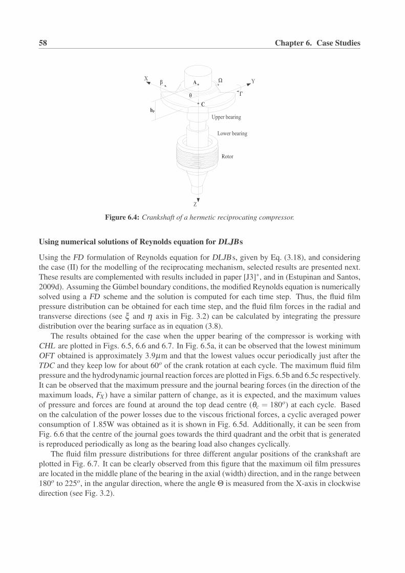
58 Chapter 6. Case Studies
Figure 6.4: Crankshaft of a hermetic reciprocating compressor.
Using numerical solutions of Reynolds equation for DLJBs
Using the FD formulation of Reynolds equation for DLJBs, given by Eq. (3.18), and consideringthe case (II) for the modelling of the reciprocating mechanism, selected results are presented next.These results are complemented with results included in paper [J3]∗, and in (Estupinan and Santos,2009d). Assuming the Gumbel boundary conditions, the modified Reynolds equation is numericallysolved using a FD scheme and the solution is computed for each time step. Thus, the fluid filmpressure distribution can be obtained for each time step, and the fluid film forces in the radial andtransverse directions (see ξ and η axis in Fig. 3.2) can be calculated by integrating the pressuredistribution over the bearing surface as in equation (3.8).
The results obtained for the case when the upper bearing of the compressor is working withCHL are plotted in Figs. 6.5, 6.6 and 6.7. In Fig. 6.5a, it can be observed that the lowest minimumOFT obtained is approximately 3.9μm and that the lowest values occur periodically just after theTDC and they keep low for about 60o of the crank rotation at each cycle. The maximum fluid filmpressure and the hydrodynamic journal reaction forces are plotted in Figs. 6.5b and 6.5c respectively.It can be observed that the maximum pressure and the journal bearing forces (in the direction of themaximum loads, FX ) have a similar pattern of change, as it is expected, and the maximum valuesof pressure and forces are found at around the top dead centre (θc = 180o) at each cycle. Basedon the calculation of the power losses due to the viscous frictional forces, a cyclic averaged powerconsumption of 1.85W was obtained as it is shown in Fig. 6.5d. Additionally, it can be seen fromFig. 6.6 that the centre of the journal goes towards the third quadrant and the orbit that is generatedis reproduced periodically as long as the bearing load also changes cyclically.
The fluid film pressure distributions for three different angular positions of the crankshaft areplotted in Fig. 6.7. It can be clearly observed from this figure that the maximum oil film pressuresare located in the middle plane of the bearing in the axial (width) direction, and in the range between180o to 225o, in the angular direction, where the angle Θ is measured from the X-axis in clockwisedirection (see Fig. 3.2).

6.1 Application to the upper bearing of a hermetic reciprocating compressor - HRC 59
N
Crank angle [deg]
(c) Journal bearing forces
Fx Fy
Crank angle [deg]
μm
(a) Minimum fluid film thickness (hmin)
Crank angle [deg]
MPa
(b) Maximum Pressure (Pmax)
Crank angle [deg]
(d) Power losses
W
Wavg
0 180 360 540 720 900 1080 1260
0 180 360 540 720 900 1080 12600 180 360 540 720 900 1080 1260
0 180 360 540 720 900 1080 12601.6
1.8
2
2.2
0
1
2
3
4
5
3
6
9
12
15
0
100
200
300
Figure 6.5: Main upper bearing parameters - CHL.
[μm]
[μm]
Y
X
Crank angle
90o
180o
270o
360o
450o
540o
630o
720o
-15-12-9-6-3
-15
-12
-9
-6
-3
Figure 6.6: Journal orbit - CHL.
Θ [degrees]z [mm]
P[M
Pa]
(b) θc = 270o (φ = 245o); Fb = 53 N
Θ [degrees]z [mm]
P[M
Pa]
(c) θc = 360o (φ = 234o); Fb = 118 N
Θ [degrees]z [mm]
P[M
Pa]
(a) θc = 180o (φ = 217o); Fb = 213 N
090
180270
360
090
180270
360
090
180270
360
06
12 06
12
06
120
2
4
0
1
2
0
0.5
1
Figure 6.7: Fluid film pressure distribution - CHL.
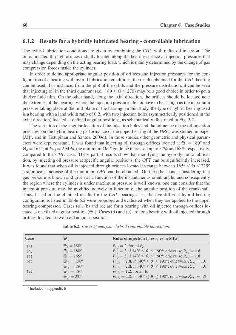
60 Chapter 6. Case Studies
6.1.2 Results for a hybridly lubricated bearing - controllable lubrication
The hybrid lubrication conditions are given by combining the CHL with radial oil injection. Theoil is injected through orifices radially located along the bearing surface at injection pressures thatmay change depending on the acting bearing load, which is mainly determined by the change of gascompression forces inside the cylinder.
In order to define appropriate angular position of orifices and injection pressures for the con-figuration of a bearing with hybrid lubrication conditions, the results obtained for the CHL bearingcan be used. For instance, from the plot of the orbits and the pressure distribution, it can be seenthat injecting oil in the third quadrant (i.e., 180 ≤ Θ ≤ 270) may be a good choice in order to get athicker fluid film. On the other hand, along the axial direction, the orifices should be located nearthe extremes of the bearing, where the injection pressures do not have to be as high as the maximumpressure taking place at the mid-plane of the bearing. In this study, the type of hybrid bearing usedis a bearing with a land width ratio of 0.2, with two injection holes (symmetrically positioned in theaxial direction) located at defined angular positions, as schematically illustrated in Fig. 3.2.
The variation of the angular location of the injection holes and the influence of the oil injectionpressures on the hybrid bearing performance of the upper bearing of the HRC, was studied in paper[J3]∗, and in (Estupinan and Santos, 2009d). In those studies other geometric and physical param-eters were kept constant. It was found that injecting oil through orifices located at Θo = 180o andΘo = 165o, at Pin j = 2 MPa, the minimum OFT could be increased up to 57% and 68% respectively,compared to the CHL case. These partial results show that modifying the hydrodynamic lubrica-tion, by injecting oil pressure at specific angular positions, the OFT can be significantly increased.It was found that when oil is injected through orifices located in range between 165o ≤ Θ ≤ 225o
a significant increase of the minimum OFT can be obtained. On the other hand, considering thatgas pressure is known and given as a function of the instantaneous crank angle, and consequentlythe region where the cylinder is under maximum pressure is well known, one can consider that theinjection pressure may be modified actively in function of the angular position of the crankshaft.Thus, based on the obtained results for the CHL bearing case, the five different hybrid bearingconfigurations listed in Table 6.2 were proposed and evaluated when they are applied to the upperbearing compressor. Cases (a), (b) and (c) are for a bearing with oil injected through orifices lo-cated at one fixed angular position (Θo). Cases (d ) and (e) are for a bearing with oil injected throughorifices located at two fixed angular positions.
Table 6.2: Cases of analysis - hybrid controllable lubrication.
Case ΘΘΘoiRules of injection (pressures in MPa)
(a) Θo = 180o Pin j = 2, for all θc
(b ) Θo = 180o Pin j = 3, if 140o ≤ θc ≤ 190o; otherwise Pin j = 1.8(c) Θo = 165o Pin j = 3, if 140o ≤ θc ≤ 190o; otherwise Pin j = 1.8(d ) Θo1 = 150o Pin j1 = 2.8, if 140o ≤ θc ≤ 190o; otherwise Pin j1 = 1.0
Θo2 = 180o Pin j2 = 2.8, if 140o ≤ θc ≤ 190o; otherwise Pin j2 = 1.0(e) Θo1 = 180o Pin j1 = 1.2, for all θc
Θo2 = 225o Pin j2 = 2.8, if 140o ≤ θc ≤ 190o; otherwise Pin j2 = 1.2
∗Included in appendix B
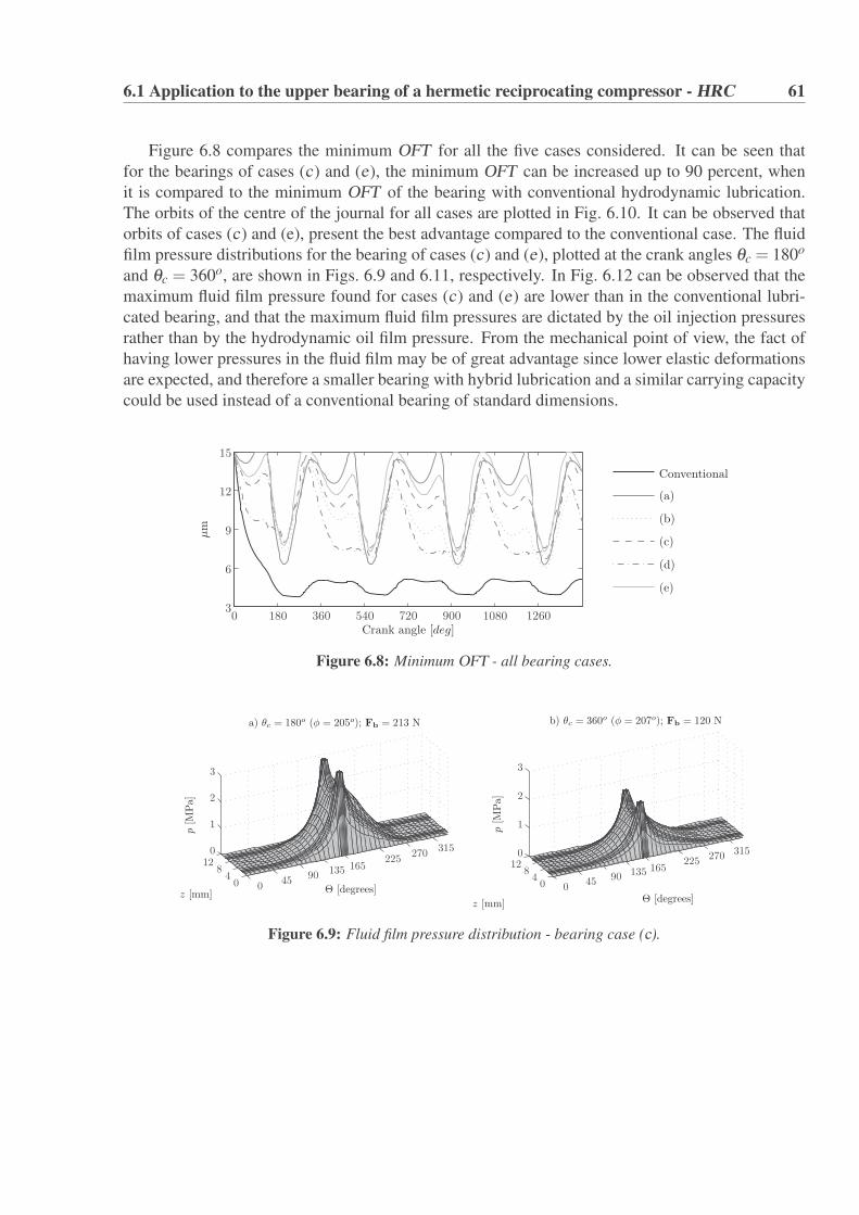
6.1 Application to the upper bearing of a hermetic reciprocating compressor - HRC 61
Figure 6.8 compares the minimum OFT for all the five cases considered. It can be seen thatfor the bearings of cases (c) and (e), the minimum OFT can be increased up to 90 percent, whenit is compared to the minimum OFT of the bearing with conventional hydrodynamic lubrication.The orbits of the centre of the journal for all cases are plotted in Fig. 6.10. It can be observed thatorbits of cases (c) and (e), present the best advantage compared to the conventional case. The fluidfilm pressure distributions for the bearing of cases (c) and (e), plotted at the crank angles θc = 180o
and θc = 360o, are shown in Figs. 6.9 and 6.11, respectively. In Fig. 6.12 can be observed that themaximum fluid film pressure found for cases (c) and (e) are lower than in the conventional lubri-cated bearing, and that the maximum fluid film pressures are dictated by the oil injection pressuresrather than by the hydrodynamic oil film pressure. From the mechanical point of view, the fact ofhaving lower pressures in the fluid film may be of great advantage since lower elastic deformationsare expected, and therefore a smaller bearing with hybrid lubrication and a similar carrying capacitycould be used instead of a conventional bearing of standard dimensions.
Crank angle [deg]
μm
Conventional
(a)
(b)
(c)
(d)
(e)
0 180 360 540 720 900 1080 12603
6
9
12
15
Figure 6.8: Minimum OFT - all bearing cases.
Θ [degrees]z [mm]
p[M
Pa]
a) θc = 180o (φ = 205o); Fb = 213 N
Θ [degrees]z [mm]
p[M
Pa]
b) θc = 360o (φ = 207o); Fb = 120 N
0 45 90 135 165225 270 315
045 90 135 165
225270 315
04
812
04
812
0
1
2
3
0
1
2
3
Figure 6.9: Fluid film pressure distribution - bearing case (c).

62 Chapter 6. Case Studies
μm
Conventional Case (a) Case (b)
μm
Case (e)
μm
Case (d)
μm
μm
Case (c)
X
Y-12-9-6-30 -12-9-6-302 -12-9-6-302
-12-9-6-302-12-9-6-302-12-9-6-302
-12
-9
-6
-3
0
-12
-9
-6
-3
0
2
-12
-9
-6
-3
0
2
-12
-9
-6
-3
0
2
-12
-9
-6
-3
0
2
-12
-9
-6
-3
0
2
Figure 6.10: Journal centre orbits - all bearing cases.
Θ [degrees]z [mm]
p[M
Pa]
a) θc = 180o (φ = 187o); Fb = 213 N
Θ [degrees]z [mm]
p[M
Pa]
b) θc = 360o (φ = 197o); Fb = 120 N
045 90 135
180 225270
315
045
90135
180225
270315
04
812
04
812 0
1
2
3
0
1
2
3
Figure 6.11: Fluid film pressure distribution - bearing case (e).
So far the performance of hybrid lubrication for the bearing compressor has been compared toCHL in terms of the minimum OFT, maximum fluid film pressure and size of orbits. However, interms of the energy consumption due to viscous friction forces, it is important to evaluate the changein the friction forces and their feasibility of being reduced by using controllable radial oil injection.Thus, using Eqs. (3.14) and (3.15) the cyclic averaged power consumption was computed for eachhybrid bearing case of Table 6.2, and is plotted in Fig. 6.13 together with the lowest value of theminimum OFT found at every crank cycle cycle. It can be seen in Fig. 6.13 that the best bearingperformance is obtained for the bearing cases (c) and (e), since for those cases thicker fluid filmsand lower power consumptions are found, when compared to the CHL bearing case. Although the

6.1 Application to the upper bearing of a hermetic reciprocating compressor - HRC 63
Crank angle [deg]
μm
(a) Minimum fluid film thickness (hmin)
Crank angle [deg]
MPa
(b) Maximum Pressure (Pmax)
Conventional
case (e)
case (c)
0 180 360 540 720 9000 180 360 540 720 9000
1
2
3
4
5
3
6
9
12
15
Figure 6.12: Comparison of minimum OFT and maximum fluid film pressures.
bearing of cases (a), (b ) and (d ), do not perform as good as the bearing of cases (c) and (e), theypresent an important advantage over the CHL bearing. The results obtained have shown that theminimum OFT in DLJBs can be notoriously increased (in this case up to 90% for case (c)) and atthe same time the friction power losses can be reduced (in this case up to 35% for case (e)), whenthe conventional hydrodynamic lubrication conditions are properly modified.
Setup
hm
in[μm]
Wavg[W
]
Wavg
hmin
(Conventional) (a) (b) (c) (d) (e)
(Conventional) (a) (b) (c) (d) (e)
1
1.1
1.2
1.3
1.4
1.5
1.6
1.7
1.8
1.93.5
4
4.5
5
5.5
6
6.5
7
7.5
8
Figure 6.13: Minimum OFT and power losses.
6.1.3 Summary of results and conclusionsIn this section the feasibility of applying controllable lubrication to the upper journal bearing of areciprocating compressor has been demonstrated through the comparison between the results ob-tained for the cases with conventional hydrodynamic lubrication and hybrid lubrication. It has tobe considered that the results presented are for specific hybrid journal bearing configurations, re-garding to the angular position of the orifices and the injection pressures. The results have shownthat the minimum OFT can be significantly increased when the oil injection pressures are modifiedas a function of the instantaneous crank angle. It was found that using for the upper bearing of ahermetic compressor a hybrid bearing with orifices located at 180o and 225o, the minimum OFT

64 Chapter 6. Case Studies
can be increased up to 90% and the energy consumption due to the viscous forces reduced up to35%. Thus, it was shown that by using simple oil injection pressure rules, synchronized with theinstantaneous crank angle, the global performance of DLJB can be improved.
6.1.4 Further remarks and technological challengesIn order to define a general methodology useful to identify optimal hybrid bearing configurationsfor different type of bearings, more detailed studies involving the variation of other geometricalfactors such as the axial land width factor, diameter and length of the orifices, bearing dimensions,etc, should be carried out. In order to be able to modify the hydrodynamics of the fluid filmsthrough radial oil injection, suitable controllable oil injection systems capable of generating theoil pressures required for the injection and with the possibility of being adapted according to thecompressor operating conditions has yet to be defined. Moreover, such a system must fulfil theconstraints in cost and compactness typical of these type of machines. In fact, the use of externaloil pumps for the conventional lubrication system of HRCs is uncommon, and instead, the rotatingmotion of the crankshaft is used as the source for oil pumping. As previously shown, the oil injectionpressures required for a controllable oil injection system in a small HRCs are not very high (Pin j ≤3MPa), therefore, the use piezoelectric hydraulic pumps for the oil injection seems to be a feasiblealternative that should be considered. Although the cost of piezo-actuated systems is usually highcompared to other alternatives, some attempts to develop piezohydraulic pumps of small size andlow cost capable of deliver up to 4 MPa, have been made (Chapman et al., 2005). However in orderto improve control pressure capabilities and operability at higher frequencies, more sophisticatedpiezohydraulic pumps using active valves and capable of deliver up to 8 MPa (Lee et al., 2004),may be considered, however their high cost is still an important drawback.
Although in this study a small reciprocating compressor was used to demonstrate the feasibil-ity of applying controllable hybrid lubrication conditions to DLJBs, the results presented may beextended to main bearings of internal combustion engines, which will be covered in the next section.

6.2 Application to main bearings of internal combustion engines - ICEs 65
6.2 Application to main bearings of internal combustion engines- ICEs
The performance of main bearings in a combustion engine affects key functions such as durability,noise and vibration. Aiming to improve engine bearing performance (i.e., to reduce friction lossesand vibrations), the work presented in this section evaluates the feasibility of modifying the dynam-ics of the hydrodynamic fluid film in main journal bearings by using active/controllable lubrication,with oil injection pressures that can be modified depending on the operational conditions. In thisstudy, the dynamic behaviour of the main bearing of a medium-size four-strokes ICE is theoreticallyinvestigated when the engine operates with controllable radial oil injection using different injectionpressure control rules. Since this study is more focused on evaluating the dynamic behaviour of en-gine journal bearings than in the structural dynamics of the engine, and one of the main concerns isto evaluate the feasibility of applying active lubrication techniques to DLJBs, this theoretical inves-tigation is based on a single-cylinder combustion engine model, where the set of motion equationsof the MBD model are obtained following the methodology described in section 2.3. It is expectedthat the theoretical results obtained in this study may be extended to multiple cylinder ICEs, and tomore complex models that could involve structural engine dynamics and combustion engine dynam-ics, after further experimental validations. The performance of the main engine bearing operatingwith controllable lubrication is compared to the performance of the bearing operating with conven-tional hydrodynamic lubrication, giving some insights into the minimum OFT, maximum fluid filmpressure, viscous friction losses and maximum vibration levels. By applying controllable radial oilinjection to main bearings it is expected: a) to reduce the friction losses by increasing the OFT ; b)to reduce vibrations (i.e., result in smaller journal orbits); and c) to increase the effective carryingload area by modifying the pressure distribution profile, which can make it possible to use bearingsof smaller dimensions with similar load-carrying capacity.
The results presented in this section are complemented with the material published in (Estupinanand Santos, 2008a, 2009c,a,b, 2010). The main geometric parameters of the system are given inTable 6.3 and the curves of combustion pressures inside the cylinder for three different enginespeeds are shown in Fig. 6.14. Notice that in a four strokes engine every power stroke take placeseach two revolutions of the crankshaft.
Table 6.3: Main geometric and physical parameters - ICE.
Crank radius (rc) 51.5 [mm] Diameter of piston (Dp) 96 [mm]Aspect ratio (λ ) 0.75 Connecting rod length (l) 170 [mm] (rcr = 120 [mm])Journal clearance (cb) 30 [μm] Masses (mc, mcr, mp) 5, 1.5, 0.5 [kg]Fluid viscosity at 40oC (μ) 0.05 [Pa.s] Angular velocity (Ω) 2400; 3000; 3600 [rpm]Diameter of orifices (do) 3 [mm] Length of orifices (lo) 25mm
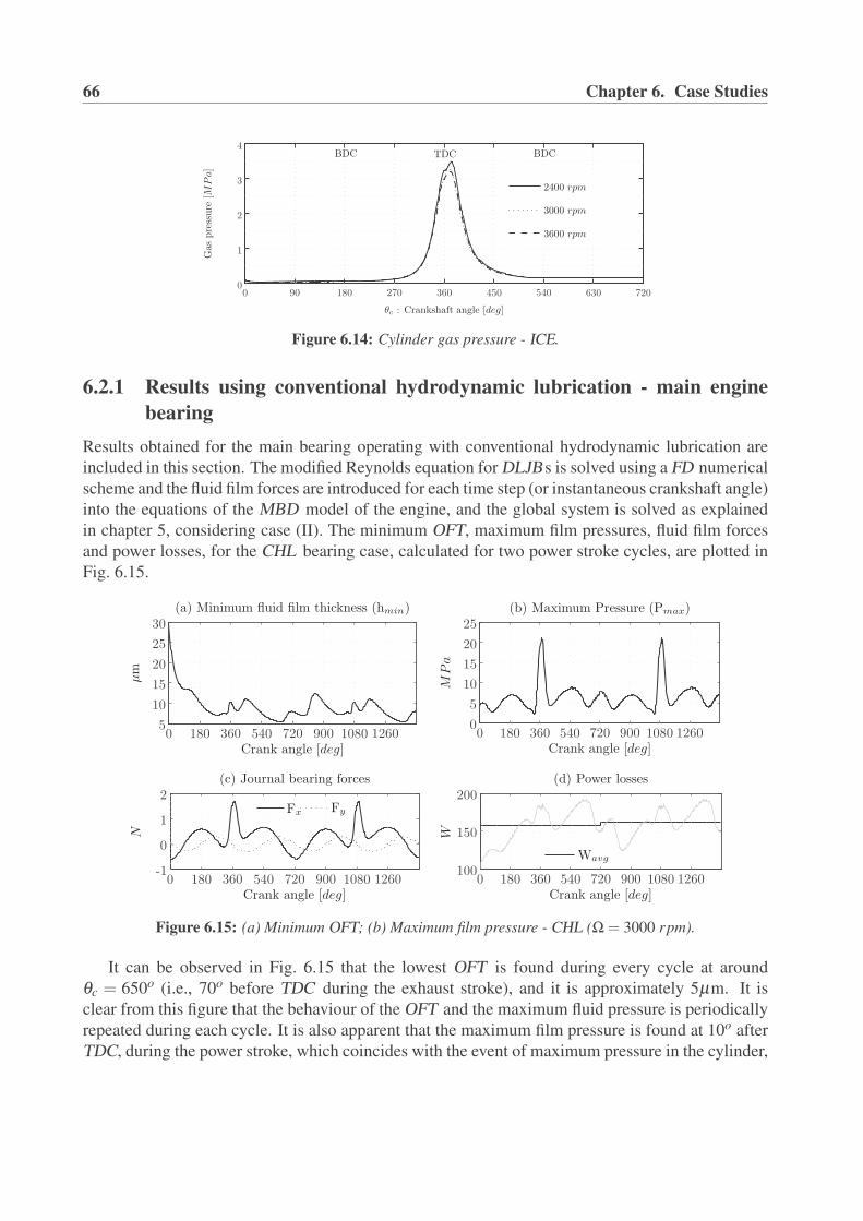
66 Chapter 6. Case Studies
θc : Crankshaft angle [deg]
Gaspressure
[MPa]
TDC BDCBDC
2400 rpm
3000 rpm
3600 rpm
0 90 180 270 360 450 540 630 7200
1
2
3
4
Figure 6.14: Cylinder gas pressure - ICE.
6.2.1 Results using conventional hydrodynamic lubrication - main enginebearing
Results obtained for the main bearing operating with conventional hydrodynamic lubrication areincluded in this section. The modified Reynolds equation for DLJBs is solved using a FD numericalscheme and the fluid film forces are introduced for each time step (or instantaneous crankshaft angle)into the equations of the MBD model of the engine, and the global system is solved as explainedin chapter 5, considering case (II). The minimum OFT, maximum film pressures, fluid film forcesand power losses, for the CHL bearing case, calculated for two power stroke cycles, are plotted inFig. 6.15.
Crank angle [deg]
μm
(a) Minimum fluid film thickness (hmin)
Crank angle [deg]
MPa
(b) Maximum Pressure (Pmax)
N
Crank angle [deg]
(c) Journal bearing forces
Crank angle [deg]
(d) Power losses
W
Fx Fy
Wavg
0 180 360 540 720 900 1080 12600 180 360 540 720 900 1080 1260
0 180 360 540 720 900 1080 12600 180 360 540 720 900 1080 1260
100
150
200
-1
0
1
2
0
5
10
15
20
25
5
10
15
20
25
30
Figure 6.15: (a) Minimum OFT; (b) Maximum film pressure - CHL (Ω = 3000 rpm).
It can be observed in Fig. 6.15 that the lowest OFT is found during every cycle at aroundθc = 650o (i.e., 70o before TDC during the exhaust stroke), and it is approximately 5μm. It isclear from this figure that the behaviour of the OFT and the maximum fluid pressure is periodicallyrepeated during each cycle. It is also apparent that the maximum film pressure is found at 10o afterTDC, during the power stroke, which coincides with the event of maximum pressure in the cylinder,

6.2 Application to main bearings of internal combustion engines - ICEs 67
as shown in Fig. 6.14. When the power losses due to the viscous frictional force are computed, itcan be observed from Fig. 6.15(d), that the instantaneous power dissipation is maximum when theminimum OFT is the lowest and when the maximum fluid pressure is the highest.
The fluid film pressure distributions computed at three different angular positions of the crankshaftare shown in Fig. 6.16. It should be noted that the maximum oil film pressures are located in themiddle plane of the bearing in the width direction, and in the range of 180o ≤ Θ ≤ 225o, in thecircumferential direction.
Θ [deg]z [mm]
p[M
Pa]
(b) θc = 360o (φ = 238o)
Θ [deg]z [mm]
p[M
Pa]
(c) θc = 540o (φ = 205o)
Θ [deg]z [mm]
p[M
Pa]
(a) θc = 180o (φ = 157o)
0 45 90 135 180225 270
315 360
0 45 90 135 180 225 270 315360
0 45 90 135 180 225 270 315 360
0
45 0
450
450
5
10
0
5
10
0
10
20
Figure 6.16: Fluid film pressure distribution - CHL (Ω = 3000 rpm).
Fig. 6.17 shows the journal centre orbits obtained for three different crankshaft rotational speeds,whose shapes agree with typical orbits of engine journal bearings found in the literature, as illus-trated in Fig. 6.18, where selected theoretical and experimental orbits are shown.
(a) 2400 rpm, vrms = 3.66mm/s
μm
X
Y
(c) 3600 rpm, vrms = 6.54mm/s
μm
X
Y
90o
180o
270o
360o
450o
540o
630o
720o
(b) 3000 rpm, vrms = 4.89mm/s
μm
X
Y
θc : Crank angle
-30-20-10102030 -30-20-10102030-30-20-10102030
-30
-20
-10
10
20
30
-30
-20
-10
10
20
30
-30
-20
-10
10
20
30
Figure 6.17: Journal center orbits - CHL (Ω = 2400; 3000; 3600 [rpm]).
Another way of representing the movement of the journal centre throughout every combustioncycle is shown in Fig. 6.19, where eccentricity ratio and attitude angle are plotted as a function ofthe instantaneous crankshaft angle. Notice that eccentricity ratio and minimum OFT are related by:ε = 1− h/cb. Thus, the lower the minimum OFT, the closer the value of eccentricity ratio to 1.In Fig. 6.19, one can observe that when the highest values of ε are found the attitude angle is inthe range between 180 ≤ φ ≤ 270 (i.e., third bearing quadrant), and it occurs when the crankshafthas rotated more than 360o (i.e., during the power stroke), with the maximum value of ε found atθc = 650o, as confirmed from the plot of the minimum OFT in Fig. 6.15a.

68 Chapter 6. Case Studies
(a) (b)
(c)
Figure 6.18: (a) Predicted orbit for big-end connecting rod bearing of a Ruston-Hornsby 6 VEB-X engine,
using a modified short bearing theory (Ritchie, 1975); (b) Predicted and measured orbit for main engine
bearing of a Scania Vabis DS11 diesel engine, using a numerical FD scheme (White, 1989); (c) left: Dy-
namic load cycle acting on big-end bearing of a 6VEB engine; center: measured orbit; right: predicted orbit
using a semi-analytical method of solution (Dede and Holmes, 1984).
Crank Angle - θc
ε
(a)
Crank Angle - θc
φ[deg]
(b)
0 90 180 270 360 450 540 630 720 810 900 990 1080 1170 1260 1350 1440
0 90 180 270 360 450 540 630 720 810 900 990 1080 1170 1260 1350 1440
0
90
180
270
360
0
0.2
0.4
0.6
0.8
1
Figure 6.19: (a) ε: Eccentricity ratio; (b) φ : Attitude angle - CHL (Ω = 3000 rpm).
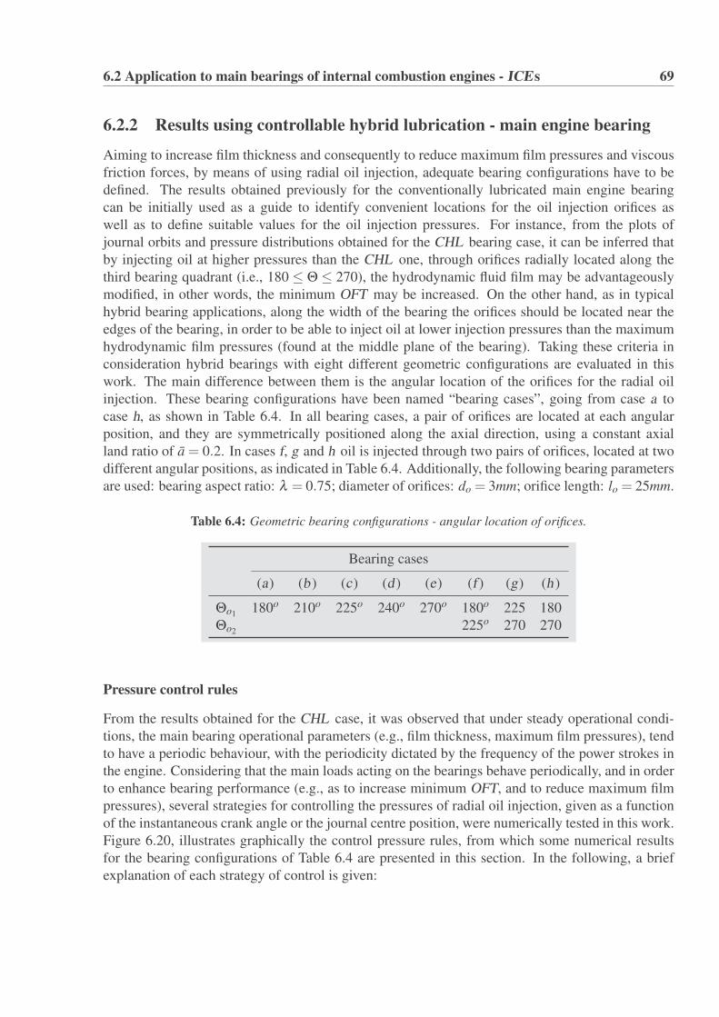
6.2 Application to main bearings of internal combustion engines - ICEs 69
6.2.2 Results using controllable hybrid lubrication - main engine bearing
Aiming to increase film thickness and consequently to reduce maximum film pressures and viscousfriction forces, by means of using radial oil injection, adequate bearing configurations have to bedefined. The results obtained previously for the conventionally lubricated main engine bearingcan be initially used as a guide to identify convenient locations for the oil injection orifices aswell as to define suitable values for the oil injection pressures. For instance, from the plots ofjournal orbits and pressure distributions obtained for the CHL bearing case, it can be inferred thatby injecting oil at higher pressures than the CHL one, through orifices radially located along thethird bearing quadrant (i.e., 180 ≤ Θ ≤ 270), the hydrodynamic fluid film may be advantageouslymodified, in other words, the minimum OFT may be increased. On the other hand, as in typicalhybrid bearing applications, along the width of the bearing the orifices should be located near theedges of the bearing, in order to be able to inject oil at lower injection pressures than the maximumhydrodynamic film pressures (found at the middle plane of the bearing). Taking these criteria inconsideration hybrid bearings with eight different geometric configurations are evaluated in thiswork. The main difference between them is the angular location of the orifices for the radial oilinjection. These bearing configurations have been named “bearing cases”, going from case a tocase h, as shown in Table 6.4. In all bearing cases, a pair of orifices are located at each angularposition, and they are symmetrically positioned along the axial direction, using a constant axialland ratio of a = 0.2. In cases f, g and h oil is injected through two pairs of orifices, located at twodifferent angular positions, as indicated in Table 6.4. Additionally, the following bearing parametersare used: bearing aspect ratio: λ = 0.75; diameter of orifices: do = 3mm; orifice length: lo = 25mm.
Table 6.4: Geometric bearing configurations - angular location of orifices.
Bearing cases
(a) (b ) (c) (d ) (e) (f ) (g) (h )
Θo1 180o 210o 225o 240o 270o 180o 225 180Θo2 225o 270 270
Pressure control rules
From the results obtained for the CHL case, it was observed that under steady operational condi-tions, the main bearing operational parameters (e.g., film thickness, maximum film pressures), tendto have a periodic behaviour, with the periodicity dictated by the frequency of the power strokes inthe engine. Considering that the main loads acting on the bearings behave periodically, and in orderto enhance bearing performance (e.g., as to increase minimum OFT, and to reduce maximum filmpressures), several strategies for controlling the pressures of radial oil injection, given as a functionof the instantaneous crank angle or the journal centre position, were numerically tested in this work.Figure 6.20, illustrates graphically the control pressure rules, from which some numerical resultsfor the bearing configurations of Table 6.4 are presented in this section. In the following, a briefexplanation of each strategy of control is given:

70 Chapter 6. Case Studies
Crank angle - θc [deg]
320 420 720
0
PinjL
PinjH
(a) control pressure rule - R1
Crank angle - θc [deg]
270 540 720
0
PinjH
(b) control pressure rule - R2
Crank angle - θc [deg]
540 720
0
PinjH
(c) control pressure rule - R3
Attitude angle - φ [deg]180 270 360
0
PinjH
(d) control pressure rule - R4
Figure 6.20: Rules for controlling oil injection pressures.
Pressure control rule R1, using this strategy, oil is injected through the orifices at two differentpressure values depending on the crankshaft angle. A higher oil pressure Pin jH is used for theinjection during the crank angular interval at which the combustion forces inside the cylinder arehigher (i.e., 320 ≤ θc ≤ 420 [deg]), as seen in Fig. 6.14. In order to keep a thicker OFT throughoutthe entire cycle, oil is injected at a lower pressure Pin jL (but higher than the CHL one) during therest of the crank cycle, as illustrated in Fig. 6.20a.
Pressure control rule R2, using this strategy, oil is injected at the pressure Pin jH during the crankangular interval at which the maximum combustion forces are found at every crank cycle, but in con-trast to R1 oil is injected during a wider angular interval at every cycle (i.e., 270 ≤ θc ≤ 540 [deg]),and there is not oil injection at a lower pressure during the rest of the crank cycle, as illustrated inFig. 6.20b.
Pressure control rule R3, this strategy aims to increase the minimum OFT by injecting oil duringthe crank angular interval at which the lowest values of OFT were found for the CHL bearingcase. Thus, using this strategy oil is injected at the pressure Pin jH during the crank angular interval540 ≤ θc ≤ 720 [deg], as illustrated in Fig. 6.20c.
Pressure control rule R4, in contrast to the previous pressure control strategies proposed, in thisstrategy oil injection is controlled as a function of the attitude angle. It was found for the CHLbearing case that the centre of the journal tends to be mostly positioned inside the third quadrantof the bearing (180 ≤ φ ≤ 270) where also the lowest OFT during every cycle is found, as it canbe noticed in the curves of eccentricity and attitude angle in Fig. 6.19, and in the orbits shownin Fig. 6.17. Thus, using control pressure rule R4, oil is injected at the pressure Pin jH when the

6.2 Application to main bearings of internal combustion engines - ICEs 71
instantaneous position of the journal centre is in the third quadrant of the bearing (i.e., when 180 ≤φ ≤ 270, according to Fig. 4.3).
Evaluation of bearing configurations and pressure control rules.
In this section, the hybrid bearing performance for the bearing configurations listed in Table 6.4,using the control pressure rules R1 to R4 shown in Fig. 6.20, is analyzed through results obtainedfrom numerical simulations. The numerical tests were carried out considering different values forthe oil injection pressures. In order to facilitate the comparison between the hybrid bearing cases tothe CHL case, the following dimensionless variables are used for the plots:
hmin =hmin
cb; pmax =
pmax
pCHLmax
; Wavg =Wavg
WCHLavg
(6.1)
where pCHLmax = 17.7 MPa and WCHL
avg = 172 W, are the values of the highest pressure and cyclicaveraged power consumption, respectively, for the conventionally hydrodynamic lubricated bearingcase. For all bearing geometric configurations and control pressure rules, Figs. 6.21, 6.22 and 6.23show the behaviour of lowest OFT, maximum film pressure and cyclic averaged power consumption,respectively, as a function of the oil injection pressures Pin jH .
hm
in
PinjH - [MPa]
R1
a b c d e f g h CHL
hm
in
PinjH - [MPa]
R2
hm
in
PinjH - [MPa]
R3
hm
in
PinjH - [MPa]
R4
6 8 10 126 8 10 12
6 8 10 126 8 10 12
0.2
0.25
0.3
0.35
0.4
0.45
0.2
0.25
0.3
0.35
0.4
0.45
0.2
0.25
0.3
0.35
0.4
0.45
0.2
0.25
0.3
0.35
0.4
0.45
Figure 6.21: Minimum OFT - all bearing cases.
In terms of the minimum OFT, it can be observed from Fig. 6.21 that the lowest OFTs are foundfor the bearing of case f using the pressure control rules R1, R2 and R4. Although the bearingconfiguration of case a is not as good as case f, it also presents a good advantage compared to theCHL case. On the other hand, it can be seen that the bearing of case e is not a good configuration,

72 Chapter 6. Case Studies
pm
ax
PinjH - [MPa]
R2
a b c d e f g h
pm
ax
PinjH - [MPa]
R3
pm
ax
PinjH - [MPa]
R4
pm
ax
PinjH - [MPa]
R1
6 8 10 12
6 8 10 126 8 10 12
6 8 10 120.5
0.75
1
1.25
0.5
0.75
1
1.25
0.5
0.75
1
1.25
0.5
0.75
1
1.25
Figure 6.22: Maximum fluid film pressure - all bearing cases.
since the minimum OFT can be even reduced, as shown in the graphs for control pressure rules R1and R2.
In terms of the maximum film pressures, it can be seen in Fig. 6.22 that in most of the hybridbearing cases analyzed, the maximum oil film pressures found are lower than in the CHL case.When control pressure rule R3 is considered, an increase in the maximum film pressure can benoticed. In cases where CHL is properly combined with oil injection, the oil film pressure is builtup over a wider bearing area, requiring consequently lower pressures to support the same bearingload conditions.
In terms of the energy consumption due to the viscous friction forces, it can be seen in Fig. 6.23,that a reduction up to 40% can be reached compared to the CHL bearing case (e.g., as in case f withcontrol rule R1).
So far, the analysis have been made with focus on the behaviour of global values of main bearingparameters, comparing between different hybrid bearing cases based on the maximum or minimumvalues found. Such an analysis helps to identify which cases present advantage compared to theothers. However, it is also relevant to know main bearing performance during every crankshaftcycle, in order to identify, for instance, possibilities for improvement. Figure 6.24 shows the orbitsfor the bearing configurations a and f using Pin jH = 8 MPa. It can be noticed in this figure that for thehybrid bearing cases analyzed, the orbital movements of the journal centre have lower eccentricitywhen compared to the CHL bearing case (plotted in light gray colour in the figure). The orbitsobtained for bearing case f present a more significant change in the orbital shape than the orbits ofbearing case a, when compared to the CHL bearing case.

6.2 Application to main bearings of internal combustion engines - ICEs 73
Wavg
PinjH - [MPa]
R2
a b c d e f g h
Wavg
PinjH - [MPa]
R3W
avg
PinjH - [MPa]
R4
Wavg
PinjH - [MPa]
R1
6 8 10 12
6 8 10 126 8 10 12
6 8 10 120.5
0.6
0.7
0.8
0.9
1
0.5
0.6
0.7
0.8
0.9
1
0.5
0.6
0.7
0.8
0.9
1
0.5
0.6
0.7
0.8
0.9
1
Figure 6.23: Cyclic averaged power consumption - all cases.
R1
(b) Orbits case f
R3
μm
R2
R4
μm
R1 R2
X
Y
R3
μm
R4
μm
(a) Orbits case a
-30-1501530-30-15015 -30-1501530-30-1501530
-30
-15
0
15
-30
-15
0
15
30-30
-15
0
15
30
-30
-15
0
15
30
Figure 6.24: Journal orbits - bearing cases a and f, using Pin jH= 8 MPa (The light gray colour corresponds
to the orbit for the CHL bearing case).

74 Chapter 6. Case Studies
Figure 6.25 shows minimum OFT and maximum film pressure as a function of the crank angle,computed during two power strokes, and considering case f -R1. It can be observed that whenPin jH = 6 MPa, the lowest value of h is hardly modified, however, when Pin jH becomes higher asignificant change in the minimum OFT compared to the CHL bearing case can be obtained, andmaximum film pressures are lowered.
Crank angle - θc [deg]
h
(a)
PinjH = 6MPa PinjH = 8MPa PinjH = 10MPa CHL
Crank angle - θc [deg]
pm
ax[M
Pa]
(b)
PinjH = 8MPa
CHL PinjH = 6MPa
PinjH = 10MPa
0 180 360 540 720 900 1080 1260
0 180 360 540 720 900 1080 1260
0
5
10
15
20
0
0.2
0.4
0.6
0.8
1
Figure 6.25: (a) Minimum OFT; (b) Maximum film pressure - bearing case f-R1.
In order to visualize how each pressure control rule can differently modify minimum OFT andmaximum film pressure, Fig. 6.26 shows the results obtained for hybrid bearing case a using controlpressure rules R1 to R4. It can be observed in Fig. 6.26 that for bearing case a, the less significantchange in OFT is found when control pressure rule R3 is used. Likewise, it can be noticed thatthe most significant change in OFT, in the interval 540 ≤ θc ≤ 720 (i.e., where the lowest OFTwas found for the CHL bearing case), is found when control pressure rules R2 and R4 are used.However, it can also be noticed that using control pressure rule R4 demands more oil injectionevents per cycle, and higher film pressures than the CHL during several crank angle intervals percycle.
In order to visualize how the pressure distribution of the fluid film is influenced by the locationof the injection orifices along the bearing surface, Fig. 6.27 shows the film pressure distribution forall cases using control pressure rule R2. The film pressure distributions are computed at θc = 360o,that is, in the region where maximum load is acting on the bearing, and therefore, high fluid filmpressures to compensate such loads are expected. From Fig. 6.27 one can noticed that the pressuredistributions obtained for bearing configurations of cases d and e do not have an important effecton the modification of the CHL pressure distribution. In fact it was shown in Fig. 6.21 that usingbearing case e-R2, the minimum OFT is lower than in the CHL bearing case. From all hybridbearing cases, it can be seen that the pressure distributions are more uniformly distributed for cases

6.2 Application to main bearings of internal combustion engines - ICEs 75
Crank angle - θc [deg]
h
Crank angle - θc [deg]
pm
ax[M
Pa]
R1 CHL
0 180 360 540 720 900 1080 1260
0 180 360 540 720 900 1080 1260
0
5
10
15
20
0.2
0.4
0.6
0.8
1
(a) using control pressure rule - R1
Crank angle - θc [deg]
h
Crank angle - θc [deg]
pm
ax[M
Pa]
R2 CHL
0 180 360 540 720 900 1080 1260
0 180 360 540 720 900 1080 1260
0
5
10
15
20
0.2
0.4
0.6
0.8
1
(b) using control pressure rule - R2
Crank angle - θc [deg]
h
Crank angle - θc [deg]
pm
ax[M
Pa]
R3 CHL
0 180 360 540 720 900 1080 1260
0 180 360 540 720 900 1080 1260
0
5
10
15
20
0.2
0.4
0.6
0.8
1
(c) using control pressure rule - R3
Crank angle - θc [deg]
h
Crank angle - θc [deg]
pm
ax[M
Pa]
R4 CHL
0 180 360 540 720 900 1080 1260
0 180 360 540 720 900 1080 1260
0
5
10
15
20
0.2
0.4
0.6
0.8
1
(d) using control pressure rule - R4
Figure 6.26: Minimum OFT and maximum film pressures for bearing case a, using different control pressure
rules (Pin jH = 10 MPa; Pin jL = 5 MPa).

76 Chapter 6. Case Studies
Θ [deg]z [mm]
p[M
Pa]
case a
Θ [deg]z [mm]
p[M
Pa]
case b
Θ [deg]z [mm]
p[M
Pa]
case c
Θ [deg]z [mm]
p[M
Pa]
case d
Θ [deg]z [mm]
p[M
Pa]
case e
Θ [deg]z [mm]
p[M
Pa]
case f
Θ [deg]z [mm]
p[M
Pa]
case g
Θ [deg]z [mm]
p[M
Pa]
case h
Θ [deg]z [mm]
p[M
Pa]
case CHL
0 45 90 135 180 225 270 315
0 45 90 135 180 225 270 315
0 45 90 135 180 225 270 315
0 45 90 135 180 225 270 315
0 45 90 135 180 225 270 315
0 45 90 135 180 225 270 315
0 45 90 135 180 225 270 315
0 45 90 135 180 225 270 315
0 45 90 135 180 225 270 315
0
45
0
45
0
45
0
45
0
45
0
45
0
45
0
45
0
45
0
10
20
0
5
10
15
0
5
10
15
0
5
10
15
0
5
10
15
0
5
10
15
0
5
10
15
0
5
10
15
0
5
10
15
Figure 6.27: Fluid film pressure distribution at θc = 360o - all cases using control pressure rule R2 (Pin jH=
10 MPa).
a, f and h. In order to illustrate how the pressure distribution of a hybrid bearing varies duringeach engine combustion cycle, due to the bearing load condition and to the injection pressure rules,Figs. 6.28 and 6.29 show the pressure distributions for cases a and f, calculated at three differentcrankshaft angles (θc = 180o; 360o and 540o), using control pressure rules R1 and R4. As expected,the higher fluid film pressures are found for θc
∼= 360o (i.e., near T DC during the power stroke ateach combustion cycle). Although the pressure distributions obtained are different depending oneach hybrid bearing case and on the control pressure rule selected, the fluid film forces have toequilibrate the load acting on the bearing at any time during each cycle. This can be noticed fromFigs. 6.28 and 6.29, which shows the computed bearing force Fb for each case, which is calculatedby integrating the pressure distribution along the bearing surface, obtaining equivalent fluid filmbearing forces (Fb) for all cases.
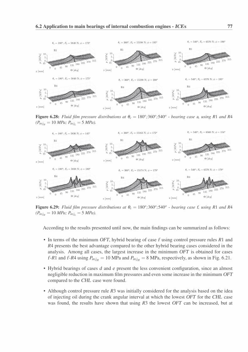
6.2 Application to main bearings of internal combustion engines - ICEs 77
Θ [deg]z [mm]
p[M
Pa]
θc = 180o; Fb = 5840 N; φ = 173o
R1
Θ [deg]z [mm]
p[M
Pa]
θc = 360o; Fb = 15198 N; φ = 195o
R1
Θ [deg]z [mm]
p[M
Pa]
θc = 540o; Fb = 6570 N; φ = 196o
R1
Θ [deg]z [mm]
p[M
Pa]
θc = 180o; Fb = 5840 N; φ = 175o
R4
Θ [deg]z [mm]p[M
Pa]
θc = 360o; Fb = 15198 N; φ = 208o
R4
Θ [deg]z [mm]
p[M
Pa]
θc = 540o; Fb = 6570 N; φ = 195o
R4
0 45 90 135 180 225 270 315
0 45 90 135 180 225 270 315
0 45 90 135 180 225 270 315
0 45 90 135 180 225 270 315
0 45 90 135 180 225 270 315
0 45 90 135 180 225 270 315
0
45
0
450
45
0
45
0
45
0
45
0
5
10
0
5
10
0
5
10
0
5
10
0
5
10
0
5
10
Figure 6.28: Fluid film pressure distributions at θc = 180o;360o;540o - bearing case a, using R1 and R4(Pin jH
= 10 MPa; Pin jL= 5 MPa).
Θ [deg]z [mm]
p[M
Pa]
θc = 180o; Fb = 5836 N; φ = 145o
R1
Θ [deg]z [mm]
p[M
Pa]
θc = 360o; Fb = 15163 N; φ = 172o
R1
Θ [deg]z [mm]
p[M
Pa]
θc = 540o; Fb = 6560 N; φ = 154o
R1
Θ [deg]z [mm]
p[M
Pa]
θc = 180o; Fb = 5838 N; φ = 180o
R4
Θ [deg]z [mm]
p[M
Pa]
θc = 360o; Fb = 15174 N; φ = 179o
R4
Θ [deg]z [mm]
p[M
Pa]
θc = 540o; Fb = 6570 N; φ = 179o
R4
0 45 90 135 180 225 270 315
0 45 90 135 180 225 270 315
0 45 90 135 180 225 270 315
0 45 90 135 180 225 270 315
0 45 90 135 180 225 270 315
0 45 90 135 180 225 270 315
0
45
0
450
45
0
45
0
45
0
45
0
5
10
0
5
10
0
5
10
0
5
10
0
5
10
0
5
10
Figure 6.29: Fluid film pressure distributions at θc = 180o;360o;540o - bearing case f, using R1 and R4(Pin jH
= 10 MPa; Pin jL= 5 MPa).
According to the results presented until now, the main findings can be summarized as follows:
• In terms of the minimum OFT, hybrid bearing of case f using control pressure rules R1 andR4 presents the best advantage compared to the other hybrid bearing cases considered in theanalysis. Among all cases, the largest increase in the minimum OFT is obtained for casesf -R1 and f -R4 using Pin jH = 10 MPa and Pin jH = 8 MPa, respectively, as shown in Fig. 6.21.
• Hybrid bearings of cases d and e present the less convenient configuration, since an almostnegligible reduction in maximum film pressures and even some increase in the minimum OFTcompared to the CHL case were found.
• Although control pressure rule R3 was initially considered for the analysis based on the ideaof injecting oil during the crank angular interval at which the lowest OFT for the CHL casewas found, the results have shown that using R3 the lowest OFT can be increased, but at

78 Chapter 6. Case Studies
expenses of reducing OFT at other times during each cycle, as shown in Fig. 6.26cc. It wasalso found that using R3 maximum film pressures can be even increased compared to the CHLbearing case.
• The energy consumption due to friction viscous forces can be lowered up to 40%, as foundfor hybrid bearing case f -R1. It was shown in Fig. 6.23 that the higher the injection pressuresthe lower the viscous friction forces. However one has to consider that using higher injectionpressure demands higher energy requirements from the injection system. Thus, if Wavg iscompared for cases f -R1 and f -R2, as shown in Fig. 6.23, one can noticed that the samereduction in energy is obtained, however, using R2 less energy is required for the injection,since the oil is injected only during a short interval at each cycle, while using R1 oil is injectedthroughout the entire cycle, as illustrated in Fig. 6.20.
• Although control pressure rule R4 gives good performance in terms of increasing minimumOFT, particularly for cases a and f, Fig. 6.26d also shows that oil injection is required duringmore time throughout each crankshaft cycle.
Results using pressure control rule R1
Selected results using control pressure rule R1 and using oil injection pressures that were adjustedafter several numerical simulations, are presented here. Extended results are included in (Estupinanand Santos, 2008a, 2009a). The minimum OFT and maximum film pressures for the CHL bearingcase and for bearing configurations a and f are plotted as a function of the crank angle during twopower strokes in Fig. 6.30. It can be seen in this figure that the predicted minimum OFT for bearingcases a and f are significantly thicker than those of the CHL bearing case. It can also be noted thatthe maximum values of the film pressures for bearing cases a and f, are smaller than those of theCHL bearing case, and that they correspond to the maximum values of oil injection pressures duringeach cycle. Figure 6.31 shows a plot of the film pressure distribution for bearing case f, plotted atthree different crank angles.
θc : Crank angle [deg]
h[μm]
(a)
θc : Crank angle [deg]
pm
ax[M
Pa]
(b)CHL case (a) case (f) CHL case (a) case (f)
0 180 360 540 720 900 1080 12600 180 360 540 720 900 1080 12600
5
10
15
20
0
10
20
30
Figure 6.30: (a) Minimum OFT; (b) Maximum pressure - controllable lubrication using R1 (Pin jH/L= 15/6
MPa for bearing case a; Pin jH/L= 12/5 MPa for bearing case f).
The predicted journal centre orbits using control pressure rule R1 and for two different opera-tional speeds are shown in Fig. 6.32. In the same plots the orbits for the CHL case are shown in
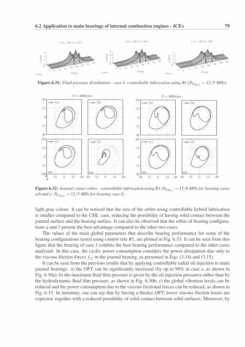
6.2 Application to main bearings of internal combustion engines - ICEs 79
Θ [deg]z [mm]
p[M
Pa]
(b) θc = 360o (φ = 238o)
Θ [deg]z [mm]
p[M
Pa]
(c) θc = 540o (φ = 205o)
Θ [deg]z [mm]
p[M
Pa]
(a) θc = 180o (φ = 157o)
045
90135
180225
270315
045
90135
180225
270315
045
90135
180225
270315
0
45
0
45
0
450
2
4
6
0
2
4
6
0
5
10
15
Figure 6.31: Fluid pressure distribution - case f: controllable lubrication using R1 (Pin jH/L= 12/5 MPa).
case (a)
Ω = 3600rpm
case (c)
μm
case (b)
case (f)
μm
case (a) case (b)
X
Y
case (c)
μm
case (f)
μm
Ω = 3000rpm
-30-1501530-30-15015 -30-1501530-30-1501530
-30
-15
0
15
-30
-15
0
15
30
-30
-15
0
15
30
-30
-15
0
15
30
Figure 6.32: Journal center orbits - controllable lubrication using R1 (Pin jH/L= 15/6 MPa for bearing cases
a,b and c; Pin jH/L= 12/5 MPa for bearing case f).
light gray colour. It can be noticed that the size of the orbits using controllable hybrid lubricationis smaller compared to the CHL case, reducing the possibility of having solid contact between thejournal surface and the bearing surface. It can also be observed that the orbits of bearing configura-tions a and f present the best advantage compared to the other two cases.
The values of the main global parameters that describe bearing performance for some of thebearing configurations tested using control rule R1, are plotted in Fig. 6.33. It can be seen from thisfigure that the bearing of case f exhibits the best bearing performance compared to the other casesanalyzed. In this case, the cyclic power consumption considers the power dissipation due only tothe viscous friction forces fv f in the journal bearing, as presented in Eqs. (3.14) and (3.15).
It can be seen from the previous results that by applying controllable radial oil injection to mainjournal bearings: a) the OFT can be significantly increased (by up to 90% in case e, as shown inFig. 6.30a); b) the maximum fluid film pressure is given by the oil injection pressures rather than bythe hydrodynamic fluid film pressure, as shown in Fig. 6.30b; c) the global vibration levels can bereduced and the power consumption due to the viscous frictional forces can be reduced, as shown inFig. 6.33. In summary, one can say that by having a thicker OFT, lower viscous friction losses areexpected, together with a reduced possibility of solid contact between solid surfaces. Moreover, by

80 Chapter 6. Case Studies
hm
in[μm]
v rm
s[m
m/s]
Wavg[W
]
Conventionallubrication
cases - controllable lubrication using R1
pm
ax[M
Pa]
Ω = 3000 rpm
Ω = 3600 rpm
CHL (a) (b) (c) (f)
CHL (a) (b) (c) (f)
10
15
20
100
150
200
250
0
3
6
9
6
9
12
15
Figure 6.33: Minimum OFT (hmin) - maximum pressure (pmax) - journal vibration (vrms) - cyclic power
consumption (Wavg), using R1.
achieving a reduction in the maximum oil film pressures while keeping the same bearing carrying-load capacity, the mechanical stresses over the bearing surface may be lowered.
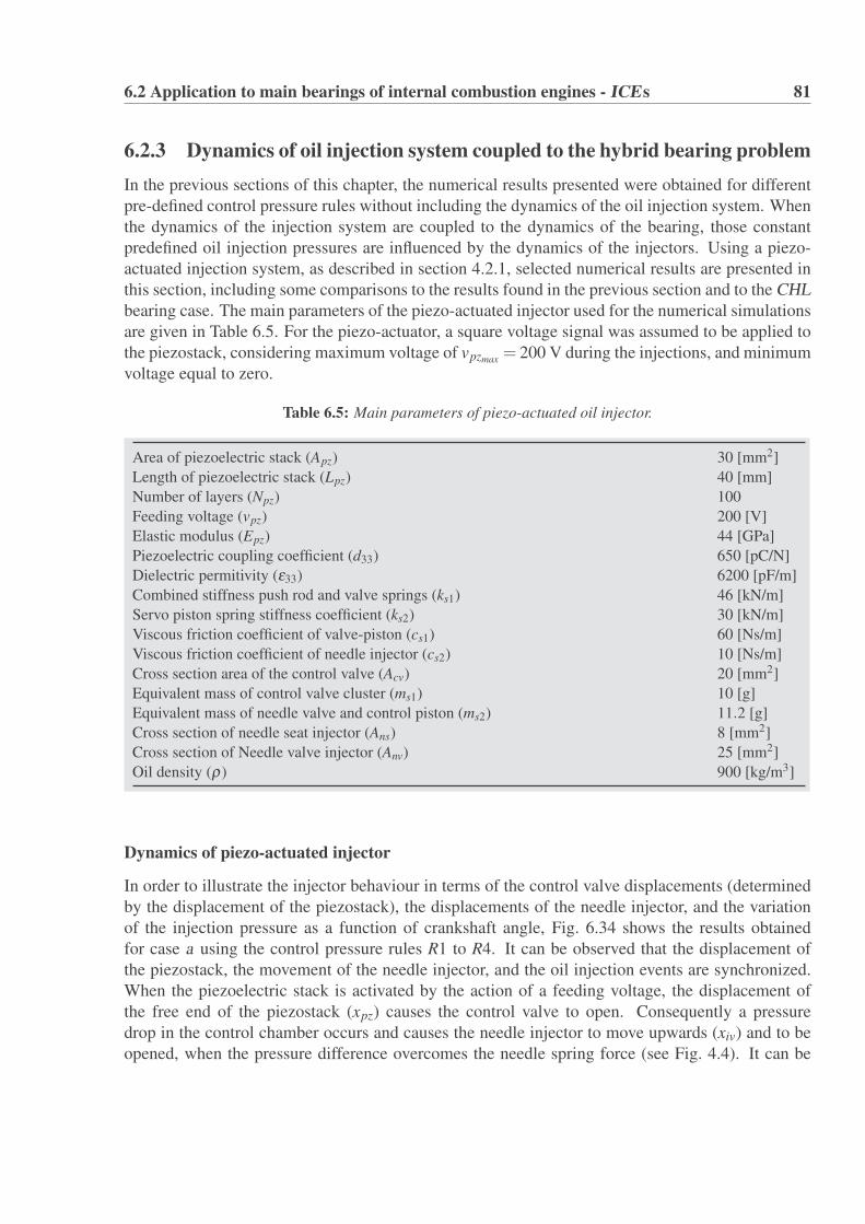
6.2 Application to main bearings of internal combustion engines - ICEs 81
6.2.3 Dynamics of oil injection system coupled to the hybrid bearing problemIn the previous sections of this chapter, the numerical results presented were obtained for differentpre-defined control pressure rules without including the dynamics of the oil injection system. Whenthe dynamics of the injection system are coupled to the dynamics of the bearing, those constantpredefined oil injection pressures are influenced by the dynamics of the injectors. Using a piezo-actuated injection system, as described in section 4.2.1, selected numerical results are presented inthis section, including some comparisons to the results found in the previous section and to the CHLbearing case. The main parameters of the piezo-actuated injector used for the numerical simulationsare given in Table 6.5. For the piezo-actuator, a square voltage signal was assumed to be applied tothe piezostack, considering maximum voltage of vpzmax = 200 V during the injections, and minimumvoltage equal to zero.
Table 6.5: Main parameters of piezo-actuated oil injector.
Area of piezoelectric stack (Apz) 30 [mm2]Length of piezoelectric stack (Lpz) 40 [mm]Number of layers (Npz) 100Feeding voltage (vpz) 200 [V]Elastic modulus (Epz) 44 [GPa]Piezoelectric coupling coefficient (d33) 650 [pC/N]Dielectric permitivity (ε33) 6200 [pF/m]Combined stiffness push rod and valve springs (ks1) 46 [kN/m]Servo piston spring stiffness coefficient (ks2) 30 [kN/m]Viscous friction coefficient of valve-piston (cs1) 60 [Ns/m]Viscous friction coefficient of needle injector (cs2) 10 [Ns/m]Cross section area of the control valve (Acv) 20 [mm2]Equivalent mass of control valve cluster (ms1) 10 [g]Equivalent mass of needle valve and control piston (ms2) 11.2 [g]Cross section of needle seat injector (Ans) 8 [mm2]Cross section of Needle valve injector (Anv) 25 [mm2]Oil density (ρ) 900 [kg/m3]
Dynamics of piezo-actuated injector
In order to illustrate the injector behaviour in terms of the control valve displacements (determinedby the displacement of the piezostack), the displacements of the needle injector, and the variationof the injection pressure as a function of crankshaft angle, Fig. 6.34 shows the results obtainedfor case a using the control pressure rules R1 to R4. It can be observed that the displacement ofthe piezostack, the movement of the needle injector, and the oil injection events are synchronized.When the piezoelectric stack is activated by the action of a feeding voltage, the displacement ofthe free end of the piezostack (xpz) causes the control valve to open. Consequently a pressuredrop in the control chamber occurs and causes the needle injector to move upwards (xiv) and to beopened, when the pressure difference overcomes the needle spring force (see Fig. 4.4). It can be

82 Chapter 6. Case Studies
noticed in Fig. 6.34 that when the piezoelectric actuator is activated a transient of short duration andhighly damped can be observed. However, this effect does not have an important influence on thepressure injection events. It can also be observed that the instantaneous pressure injections, whichare calculated after the coupled system is solved, are very close to the pressure injections definedwhen the system is uncoupled.
Crank angle - θc [deg]
xpz[m
m]
Crank angle - θc [deg]
xiv
[mm]
Crank angle - θc [deg]
Pin
j[M
Pa]
0 180 360 540 720
0 180 360 540 720
0 180 360 540 720
0
5
10
15
0
0.5
1
0
0.01
0.02
(a) using control pressure rule - R1
Crank angle - θc [deg]
xpz[m
m]
Crank angle - θc [deg]
xiv
[mm]
Crank angle - θc [deg]
Pin
j[M
Pa]
0 180 360 540 720
0 180 360 540 720
0 180 360 540 720
0
5
10
15
0
0.5
1
0
0.01
0.02
(b) using control pressure rule - R2
Crank angle - θc [deg]
xpz[m
m]
Crank angle - θc [deg]
xiv
[mm]
Crank angle - θc [deg]
Pin
j[M
Pa]
0 180 360 540 720
0 180 360 540 720
0 180 360 540 720
0
5
10
15
0
0.5
1
0
0.01
0.02
(c) using control pressure rule - R3
Crank angle - θc [deg]
xpz[m
m]
Crank angle - θc [deg]
xiv
[mm]
Crank angle - θc [deg]
Pin
j[M
Pa]
0 180 360 540 720
0 180 360 540 720
0 180 360 540 720
0
5
10
15
20
0
0.5
1
0
0.01
0.02
(d) using control pressure rule - R4
Figure 6.34: Injection parameters - bearing case a. xpz: displacement of piezostack; xiv: displacement of
needle injector; Pin j: oil injection pressure. (Pin jH/L= 10/5 MPa).

6.2 Application to main bearings of internal combustion engines - ICEs 83
Numerical results with and without coupling the injection system to the hybrid bearing prob-lem
The differences in terms of the minimum OFT and the maximum film pressures, obtained for thehybrid bearing cases a-R1 and f -R1, considering an uncoupled and a coupled solution, can be seenin Fig. 6.26. Although small differences in the minimum OFT can be partially found during eachcombustion cycle, those differences are not significant for the two cases considered, as shown inFig. 6.35. Regarding to the behaviour of the maximum film pressure, the differences between theuncoupled and coupled system are negligible, except for a very small delay at the ends of the oilinjection events, which may be mainly caused by the viscous friction of the needle injector.
Crank angle - θc [deg]
h
Crank angle - θc [deg]
pm
ax[M
Pa]
R1 R1inj CHL
0 180 360 540 720
0 180 360 540 720
0
5
10
15
20
0.2
0.4
0.6
0.8
1
(a) case a, rule - R1
Crank angle - θc [deg]
h
R1 R1inj CHL
Crank angle - θc [deg]
pm
ax[M
Pa]
0 180 360 540 720 900 1080 1260
0 180 360 540 720
0
5
10
15
20
0.2
0.4
0.6
0.8
1
(b) case f, rule - R1
Figure 6.35: Minimum OFT and maximum film pressures for bearing cases a and f, with and without includ-
ing the injector dynamics (Pin jH/L= 10/5 MPa).
Evaluation of injection oil flow and power consumption
The oil flow delivered during the injections is calculated for each bearing configuration case usingEq. (4.19). The variation of oil flow delivered to the bearing through the injection holes duringa complete engine combustion cycle, is plotted in Fig. 6.36, for the bearing case a using controlpressure rules R1 to R4. It can be noticed for each case the influence of the oil injection pressure onthe amount of oil delivered during the injection events. In general, one can say that the oil injectionflow increases, when the injection pressure increases. When using control pressure rule R1, it canbe noticed in Fig. 6.36a that oil flow is delivered to the bearing through the entire cycle. It canalso be observed that the amount of oil injected may become higher during the crankshaft angularinterval at which oil is injected at the lower pressure (Pin jL). This is due to the dependency of oilflow on the pressure difference between the oil injection pressure (Pin j) and the hydrodynamic fluidfilm pressure (Pjb).
The losses of energy caused by viscous friction forces can be reduced using controllable radialoil injection. In order to evaluate the potential savings of energy, it has been calculated in percent
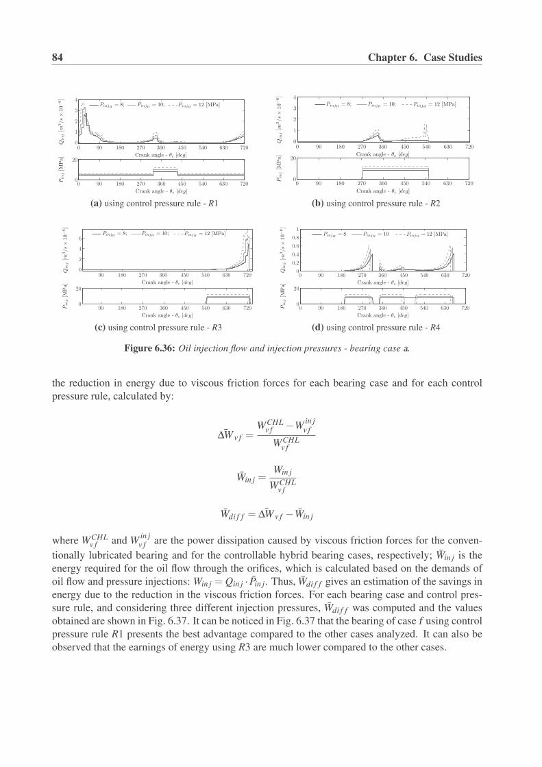
84 Chapter 6. Case Studies
Crank angle - θc [deg]
Qin
j[m
3/s
×10
−6]
PinjH = 8; PinjH = 10; PinjH = 12 [MPa]
Crank angle - θc [deg]
Pin
j[M
Pa]
0 90 180 270 360 450 540 630 720
0 90 180 270 360 450 540 630 720
0
20
0
1
2
3
4
(a) using control pressure rule - R1
Crank angle - θc [deg]
Qin
j[m
3/s
×10
−6]
Crank angle - θc [deg]
Pin
j[M
Pa]
PinjH = 8; PinjH = 10; PinjH = 12 [MPa]
0 90 180 270 360 450 540 630 720
0 90 180 270 360 450 540 630 720
0
20
0
1
2
3
4
(b) using control pressure rule - R2
Crank angle - θc [deg]
Qin
j[m
3/s
×10
−6]
Crank angle - θc [deg]
Pin
j[M
Pa]
PinjH = 8; PinjH = 10; PinjH = 12 [MPa]
90 180 270 360 450 540 630 720
90 180 270 360 450 540 630 720
0
20
0
2
4
6
(c) using control pressure rule - R3
PinjH = 8 PinjH = 10 PinjH = 12 [MPa]
Crank angle - θc [deg]Q
inj[m
3/s
×10
−6]
Crank angle - θc [deg]
Pin
j[M
Pa]
0 90 180 270 360 450 540 630 720
0 90 180 270 360 450 540 630 720
0
20
0
0.2
0.4
0.6
0.8
1
(d) using control pressure rule - R4
Figure 6.36: Oil injection flow and injection pressures - bearing case a.
the reduction in energy due to viscous friction forces for each bearing case and for each controlpressure rule, calculated by:
¯ΔW v f =WCHL
v f −Win jv f
WCHLv f
Win j =Win j
WCHLv f
Wdi f f = ¯ΔW v f −Win j
where WCHLv f and W
in jv f are the power dissipation caused by viscous friction forces for the conven-
tionally lubricated bearing and for the controllable hybrid bearing cases, respectively; Win j is theenergy required for the oil flow through the orifices, which is calculated based on the demands ofoil flow and pressure injections: Win j = Qin j · Pin j. Thus, Wdi f f gives an estimation of the savings inenergy due to the reduction in the viscous friction forces. For each bearing case and control pres-sure rule, and considering three different injection pressures, Wdi f f was computed and the valuesobtained are shown in Fig. 6.37. It can be noticed in Fig. 6.37 that the bearing of case f using controlpressure rule R1 presents the best advantage compared to the other cases analyzed. It can also beobserved that the earnings of energy using R3 are much lower compared to the other cases.

6.2 Application to main bearings of internal combustion engines - ICEs 85
Bearing case
Wdif
f[%
] (a) - R1 -
PinjH = 8 PinjH = 10 PinjH = 12 [MPa]
a b c d e f g h0
10
20
30
40
Bearing case
Wdif
f[%
]
(b) - R2 -
a b c d e f g h0
10
20
30
40
Bearing case
Wdif
f[%
]
(c) - R3 -
a b c d e f g h0
10
20
30
40
Bearing case
Wdif
f[%
]
(d) - R4 -
a b c d e f g h0
10
20
30
40
Figure 6.37: Savings in cyclic power consumption.
6.2.4 Summary of resultsThe results presented in this section for a main engine bearing operating with controllable lubri-cation have shown that the lubrication performance of main engine bearings can be significantlyenhanced by combining conventional hydrodynamic lubrication with controllable radial oil injec-tion. It was shown from the results that the fluid film thickness can be increased up to 90% andat the same time the friction losses and vibrations can be reduced up to 40%. The bearing casesthat present the best hybrid bearing performance in terms of the minimum OFT were for cases aand f, operating with control pressure rules R1 and R2. However, when the savings of energy wereanalyzed, the hybrid bearing of case f operating with control pressure rule R1 presented the bestadvantage compared to the other bearing cases.
6.2.5 Further remarks and technological challengesThe use of piezoelectric actuation for the oil injection system presents several advantages in terms ofcompactness and fast response when it is compared to mechanical unit injectors and servohydraulicoil injection systems. This type of oil injection system may be also a good substitute of active oilinjection systems operating with servohydraulic valves, which have been successfully used in otherbearing applications, such as, actively-lubricated tilting pad journal bearings (Santos and Russo,1998; Santos et al., 2004).
Further studies should be carried out in order to experimentally validate hybrid bearing perfor-mance operating with the control pressure rules proposed in this section. Although the numericalsimulations were carried out considering the main bearing of a single-cylinder ICE, similar oil in-jection strategies may be applied to main bearings of multiple cylinder combustion engines and ingeneral to other type of reciprocating machines using fluid film bearings, in order to enhance theirtribological performance.

86 Chapter 6. Case Studies

Chapter 7
Conclusions and Future Aspects
The feasibility of applying controllable lubrication to dynamically loaded journal bearings (DLJBs)was studied in this project by analyzing the behaviour of minimum oil film thickness (OFT ), maxi-mum pressure, orifices distribution over the bearing surface, oil injection pressures, friction forces,and feasible oil injection systems. It was shown that adequate hybrid bearing configurations andoil injection control rules may be defined based on the bearing performance under conventional lu-brication conditions (CHL ). Several advantages of using controllable lubrication over conventionallubrication in DLJBs were presented, mainly in terms of increasing the minimum fluid film thick-ness, increasing the effective carrying load area and lowering the viscous friction forces. In orderto control the oil injection, several strategies were evaluated, where the oil injection pressures aregiven as a function of the rotational crank angle. Two different cases were considered during thisstudy: a) main bearing of a hermetic reciprocating compressor (HRC ); b) crankshaft main bearingof a single-cylinder four-strokes internal combustion engine (ICE ). From the mathematical modelsdeveloped, their computational implementation, and the analysis of numerical results obtained forthese two particular cases of study, the main technical conclusions can be summarized as follows:
Hermetic reciprocating compressor - HRC
• From the modelling of a HRC using three different approaches, and considering CHL forthe upper and lower bearings, no significant differences were found between the three casesregarding to the estimation of the hydrodynamic journal bearing forces and the fluid film pres-sures. It was found that under CHL conditions, the maximum values of fluid film pressuresand bearing forces are found close to θc = 180o. The lowest minimum OFT is found at everycrank cycle at θc = 260o, with the orbit of the journal centre oscillating in the third bearingquadrant, as also shown in [J1],[J2], and in (Santos and Estupinan, 2007).
• The results obtained using hybrid controllable lubrication showed that the minimum OFT canbe significantly increased through radial oil injection, with controllable injection pressuresrules given as a function of the crank angle. It was found that injecting oil through orificeslocated at Θo = 180o and Θo = 225o, and with oil injection pressures varying between 2MPato 3MPa, the minimum OFT can be increased more than 90% compared to the CHL bearingcase. These results are also shown in [J3], and in (Estupinan and Santos, 2008b, 2009d).When the cyclic averaged power consumption was computed for the controllable lubricated
87
88 Chapter 7. Conclusions and Future Aspects
bearing cases, it was found a reduction in the cyclic power consumption due to the viscousfriction forces up to 35% compared to the CHL bearing case.
Internal combustion engine - ICE
• Based on the analysis made for the main engine bearing of an ICE, operating with CHL,eight geometric hybrid bearing configurations (cases a to h ) and four rules for controllingoil injection pressures (R1 to R4) were proposed in this work. It was found for the CHLbearing case that the lowest OFT is found at θc = 650o, that is, 70o before the TDC duringthe exhaust stroke (Estupinan and Santos, 2008a). Good correlation was found between thebearing orbits obtained in this work for the CHL engine bearing case, and the engine bearingorbits published in the literature.
• In general, it was found that the changes in the hydrodynamic oil film pressure, obtained bymeans of applying controllable radial oil injection, lead to significant increase of minimumOFT and reduction of viscous friction losses, however the hybrid bearing performance mustbe evaluated for each case individually, since the results are very dependent on the geometricbearing configurations, the control pressure rules and the oil injection pressures. Additionally,it was found that vibrations of crankshaft can be also reduced, which is reflected by the fact ofhaving smaller journal centre orbits when controllable lubrication is applied (Estupinan andSantos, 2009a).
• It was found that for the hybrid bearing of case f with oil injected through orifices locatedat Θo = 180o and Θo = 225o, using control pressure rule R1 (with Pin jH/L
= 12/5 MPa), theminimum OFT can be increased up to 90% compared to the CHL bearing case. This is alsoshown in (Estupinan and Santos, 2008a, 2009a).
• In terms of the minimum OFT, hybrid bearing of case f using control pressure rules R1 andR4 presents the best advantage compared to the other hybrid bearing cases considered in theanalysis. Among all cases, the largest increase in the minimum OFT was obtained for cases f -R1 and f -R4 using Pin jH = 10MPa and Pin jH = 8MPa, respectively. Inadequate hybrid bearingconfigurations were found for the bearing cases d and e (i.e., orifices located at Θo = 240o andΘo = 270o, respectively), since almost a negligible increase in the minimum OFT comparedto the CHL bearing case was found. In cases e-R1 and e-R2 the minimum OFT calculatedwas lower than in the CHL bearing case.
• From the four pressure control strategies analyzed, the results showed that the lowest OFTcan be increased using R3, but at the expense of reducing OFT at other times during eachcycle. It was also found that using R3 maximum film pressures were higher than to the CHLbearing case.
• In terms of the savings of power consumption due to the reduction of the viscous frictionforces, the best performance was obtained for bearing case f using control pressure rule R1.It was found that the energy consumption due to friction viscous forces can be reduced up to40%.

89
• Although using control pressure rule R4 gives good bearing performance in terms of increas-ing minimum OFT, particularly for cases a and f, oil injection is required during a longer timethroughout each crankshaft cycle.
• In this work two oil injection systems were described. The results obtained by coupling thedynamics of a piezo-actuated injection system to the dynamics of the main journal bearingsshowed that not significant differences were found in the behaviour of the global bearing pa-rameters. Nevertheless, it is worth to point out that the coupling of the injector dynamics to thehybrid bearing dynamics, will help in further studies to evaluate hybrid bearing performanceusing more sophisticated oil injection control rules.
As shown, through theoretical analysis and numerical simulations of CHL bearing performanceand controllable hybrid bearing performance of DLJBs, significant improvements can be obtainedapplying controllable radial oil injection. Nevertheless, further studies should be carried out inorder to experimentally evaluate the oil injection systems presented in this work. Moreover, theneed for introducing thermal effects in the modelling of main engine bearings operating with ac-tive/controllable lubrication systems, could be confirmed by comparing numerical results to exper-imental data. Additionally, bearing parametric studies should be carried out in order to be able todefine optimal geometric hybrid bearing configurations.
The feasibility study carried out in this work was based on numerical results obtained fromthe solution of a mathematical model which included the dynamics of the main components oftypical reciprocating machines, the dynamics of the bearing fluid films, and the dynamics of theoil injection. The main results were presented for the upper bearing of a HRC, and for the maincrankshaft bearing of a single-cylinder ICE, operating with CHL and active/controllable lubricationconditions. The strategies for controlling radial oil injection, and the oil injection systems presentedin this work, can be considered to be used in main bearings of multiple cylinder ICEs and in generalin other type of reciprocating machines using fluid film bearings, such as, industrial compressorsand large diesel engines. In this last case the effects of introducing radial oil injection can becomequite important in terms of reducing energy losses, since there is a high potential for reduction infriction forces.
“It is just a matter of time before active bearings will be regularly employed in machine tools, gasturbines, terrestrial turbines, engine suspensions, valve control, and various other mechanisms”(Ulbrich, 1994).

90 Chapter 7. Conclusions and Future Aspects

Bibliography
Alshaer, B., Nagarajan, H., Beheshti, H., Lankarani, H., Shivaswamy, S., 2005. Dynamics of a multibody me-chanical system with lubricated long journal bearings. Transactions of the ASME. Journal of MechanicalDesign 127 (3), 493–498.
ANSI/IEEE, 1987. IEEE standard on piezoelectricity. Tech. Rep. Std 176-1987, IEEE Ultrasonics, Ferro-electrics, and Frequency Control Society, New York.
Arnold, M., Burgermeister, B., Eichberger, A., 2007. Linearly implicit time integration methods in real-timeapplications: Daes and stiff odes. Multibody System Dynamics 17 (2-3), 99–117.
Arnold, M., Carrarini, A., Heckmann, A., Hippmann, G., 2004. Simulation techniques for multidisciplinaryproblems in vehicle system dynamics. Vehicle System Dynamics 40, 17–35.
AVL, 2009. AVL Excite Power Unit: Elastohydrodynamic contact models. Advanced Simulation Technolo-gies - Data sheet. Available at: http://www.avl.com/excite.
Backhaus, K., Knoll, G., October 2008. Oil flow interaction of engine bearings. In: Proceedings of theSTLE/ASME International Joint Tribology Conference. No. IJTC2008-71036. Miami, FL, USA.
Booker, J., 1965. Dynamically loaded journal bearings – mobility method of solution. American Society ofMechanical Engineers – Transactions – Journal of Basic Engineering 87 (3), 537–546.
Booker, J., Huebner, K., 1972. Application of finite element methods to lubrication: An engineering approach.J Lubr Technol Trans ASME 94 Ser F (4), 313–323.
Boysal, A., Rahnejat, H., 1997. Torsional vibration analysis of a multi-body single cylinder internal combus-tion engine model. Applied Mathematical Modelling 21 (8), 481–493.
Bremer, H., 1988. Dynamik und regelung mechanischer systeme. B.G. Teubner Verlag, Stuttgart, Germany.
Bremer, H., 1999. On the dynamics of elastic multibody systems. Applied Mechanics Reviews - IncludingSupplement 52 (9), 275.
Bukovnik, S., Dorr, N., Caika, V., Bartz, W., Loibnegger, B., 2006. Analysis of diverse simulation modelsfor combustion engine journal bearings and the influence of oil condition. Tribology International 39 (8),820–826.
Bukovnik, S., Offner, G., Caika, V., Priebsch, H., Bartz, W., 2007. Thermo-elasto-hydrodynamic lubricationmodel for journal bearing including shear rate-dependent viscosity. Lubrication Science 19 (4), 231–245.
91

92 Bibliography
Campbell, J., Love, P., Martin, F., Rafique, S., 1967-1968. Bearings for reciprocating machinery – reviewof present state of theoretical, experimental and service knowledge. Institution on Mechnical Engineers –Proceedings 182 (Part 3A), 51–74.
Chapman, E., Herdic, S., Keller, C. A., Lynch, C., 2005. Development of miniaturized piezo-hydraulic pumps.Proceedings of SPIE - The International Society for Optical Engineering 5762, 299–310.
Cho, J., Moon, S., 2005. A numerical analysis of the interaction between the piston oil film and the componentdeformation in a reciprocating compressor. Tribology International 38 (5), 459–468.
Choi, J., Lee, J., Han, D., 1992. Oil film thickness in engine main bearings: comparison between calculationand experiment by total capacitance method. SAE Special Publications (936), 147–160.
Chung, N.-H., Oh, B.-G., Sunwoo, M.-H., 2008. Modelling and injection rate estimation of common-railinjectors for direct-injection diesel engines. Proceedings of the Institution of Mechanical Engineers - D222 (6), 1089.
Ciulli, E., 1992. Review of internal combustion engine losses part 1: specific studies on the motion of pistons,valves and bearings. Proceedings of the Institution of Mechanical Engineers, Part D: Journal of AutomobileEngineering 206 (4), 223–236.
Craven, A., Holmes, R., 1972. The vibration of engine crankshafts-a fast numerical solution. InternationalJournal for Numerical Methods in Engineering 5 (1), 17–24.
Dede, M., Holmes, R., 1984. On prediction and experimental assessment of engine-bearing performance.Tribology International 17 (5), 251–258.
Drab, C., Engl, H., Haslinger, J., Offner, G., Pfau, R., Zulehner, W., 2009. Dynamic simulation of crankshaftmultibody systems. Multibody System Dynamics 22 (2), 133–144.
Eberhard, P., Schiehlen, W., 2006. Computational dynamics of multibody systems: history, formalisms, andapplications. Transactions of ASME. Journal of Computational and Nonlinear Dynamics 1 (1), 3–12.
Elrod, H., 1981. A cavitation algorithm. Transactions of the ASME. Journal of Lubrication Technology103 (3), 350–354.
Estupinan, E., Santos, I., September 2008a. Feasibility of applying controllable lubrication to the main bear-ings of reciprocating engines. In: Proceedings of 23rd International Conference on Noise and VibrationEngineering - ISMA 2008. Leuven, Belgium, pp. 2015–27, ISBN 978-90-7380-286-5.
Estupinan, E., Santos, I., October 2008b. Linking rigid and flexible multibody systems via thin fluid filmsactively controlled. In: Proceedings of STLE/ASME International Joint Tribology Conference - IJTC 2008.Miami (FL), USA., ISBN 978-0-7918-3837-2.
Estupinan, E., Santos, I., June 2008c. Linking rigid multibody systems via controllable thin fluid films. In:Proceedings of NORDTRIB 2008, 13th Nordic Symposium on Tribology. No. NT2008-42-30. Tampere,Finland, ISBN 978-952-15-1959-8.
Estupinan, E., Santos, I., July 5-9 2009a. Active lubrication applied to internal combustion engines - eval-uation of control strategies. In: Proceedings of the 16th International Congress on Sound and Vibration.Krakow, Poland, ISBN: 978-83-60716-71-7.
Bibliography 93
Estupinan, E., Santos, I., September 2009b. Active lubrication strategies applied to dynamically loaded fluidfilm bearings. In: Proceedings of World Tribology Conference 2009 - WTC IV. Kyoto, Japan, ISBN:978-4-9900139-9-8.
Estupinan, E., Santos, I., May 2009c. Feasibility of applying active lubrication to dynamically loaded fluidfilm bearings. In: STLE 2009 Annual Meeting. Orlando - FL, USA.
Estupinan, E., Santos, I., March 2009d. Feasibility of applying controllable lubrication to dynamically loadedjournal bearings. In: Proceedings of XIII International Symposium on Dynamic Problems of Mechanics -DINAME 2009. Angra dos Reis, RJ, Brazil.
Estupinan, E., Santos, I., January 2010. Schemes for applying active lubrication to main engine bearings. In:Proceedings of 11th Pan-American Congress of Applied Mechanics - PACAM XI. Foz do Iguacu, Brazil.
Fantino, B., Frene, J., 1985. Comparison of dynamic behavior of elastic connecting-rod bearing in both petroland diesel engines. Journal of Tribology, Transactions of the ASME 107 (1), 87–91.
Fatu, A., Hajjam, M., Bonneau, D., 2006. A new model of thermoelastohydrodynamic lubrication in dynam-ically loaded journal bearings. Transactions of the ASME. Journal of Tribology 128 (1), 85–95.
Feenstra, J., Granstrom, J., Sodano, H., 2008. Energy harvesting through a backpack employing a mechani-cally amplified piezoelectric stack. Mechanical Systems and Signal Processing 22 (3), 721–734.
Fox, R., McDonald, A., Pritchard, P., 2004. Introduction to Fluid Mechanics. John Wiley & Sons, Inc., USA.
Frene, J., Nicolas, D., Degueurce, B., Berthe, D., Godet, M., 1990. Lubrification Hydrodynamique. EditionsEyrolles, Paris.
Fridman, V., Piraner, I., Musolff, C., 2004. Some applications of the hydrodynamic and elasto-hydrodynamicanalysis to the diesel engine bearings. Proceedings of the ASME/STLE International Joint Tribology Con-ference, IJTC 2004 (PART A), 807–829.
Fuller, C., Elliot, S., Nelson, P., 1996. Active Control of Vibration. Academic Press, Inc.
Garcia de Jalon, J., Bayo, E., 1994. Kinematic and Dynamic Simulation of Multibody Systems. The Real-Time Challenge. Springer-Verlag, New-York.
Goenka, P., Oh, K., 1986. Optimum short bearing theory for the elastohydrodynamic solution of journalbearings. Journal of Tribology, Transactions of the ASME 108 (2), 294–299.
Goenka, P. K., Paranjpe, R. S., 1992. Review of engine bearing analysis methods at general motors. EngineTribology and SAE Special Publications (919), 67–75.
Goodwin, M. J., Nikolajsen, J. L., Ogrodnik, P. J., 2003. Reciprocating machinery bearing analysis: The-ory and practice. Proceedings of the Institution of Mechanical Engineers, Part J: Journal of EngineeringTribology 217 (6), 409–426.
Hamrock, B. J., 1991. Fundamental of Fluid Film Lubrication. NASA Reference Publication, USA.
Han, H. S., 2004. Web-based dynamic simulation system for multi-body systems. Advances in EngineeringSoftware 35 (2), 75–84.

94 Bibliography
Haugaard, A. M., Santos, L. F., 2009. Modeling of flexible tilting pad journal bearings with radial oil injec-tion. 2008 Proceedings of the STLE/ASME International Joint Tribology Conference, IJTC 2008, 335–337.
Heinrichson, N., Santos, I. F., 2008. Reducing friction in tilting-pad bearings by the use of enclosed recesses.Journal of Tribology 130 (1).
Heinrichson, N., Santos, I. F., Fuerst, A., 2007. The influence of injection pockets on the performance oftilting-pad thrust bearings - part i: Theory. Journal of Tribology 129 (4), 895–903.
Hirani, H., Athre, K., Biswas, S., 1998. Rapid and globally convergent method for dynamically loaded jour-nal bearing design. Proceedings of the Institution of Mechanical Engineers -J- Journal of EngineeringTribology 212 (3), 207.
Hirani, H., Athre, K., Biswas, S., 1999a. Dynamic analysis of engine bearings. International Journal ofRotating Machinery 5, 283–293.
Hirani, H., Athre, K., Biswas, S., 1999b. Dynamically loaded finite length journal bearings: Analyticalmethod of solution. Journal of Tribology, Transactions of the ASME 121 (4), 844–852.
Horikawa, O., Sato, K., Shimokohbe, A., 1992. An active air journal bearing. Nanotechnology 3 (2), 84–90.
Hountalas, D. T., Kouremenos, A. D., 1998. Development of a fast and simple simulation model for the fuelinjection system of diesel engines. Advances in Engineering Software 29 (1), 13–28.
Isermann, R., 2006. Automotive mechatronic systems - general developments and examples. Automa-tisierungstechnik 54 (9), 419–429.
Jadon, V., Singh, M., 2007. Study of supply cut-off and bearing geometric parameters on design of hybridjournal bearing. Industrial Lubrication and Tribology 59 (2), 92–102.
Katano, H., Iwamoto, A., Saitoh, T., 1991. Dynamic behaviour of internal combustion engine crankshaftunder operating conditions. In: Proceedings of IMech E Conference. paper C430/049/91. pp. 205–209.
Kawamoto, A., Inagaki, M., Aoyama, T., Mori, N., Ikeura, O., Uno, T., Yamamoto, K., 2000. Prediction ofstructural and kinematic coupled vibration on internal combustion engine. Proceedings of the 25th Inter-national Conference on Noise and Vibration Engineering - ISMA 25, 1323–1330.
Kim, B.-J., Kim, K.-W., 2001. Thermo-elastohydrodynamic analysis of connecting rod bearing in internalcombustion engine. Journal of Tribology 123 (3), 444–454.
Kim, H. J., Ahn, J. M., 2007. Numerical simulation of oil supply system of a reciprocating compressor forhousehold refrigerators. HVAC and R Research 13 (5), 833–847.
Kim, T. J., Han, J. S., 2004. Comparison of the dynamic behavior and lubrication characteristics of a re-ciprocating compressor crankshaft in both finite and short bearing models. Tribology Transactions 47 (1),61–69.
Knoll, G., Schoenen, R., Wilhelm, K., 1997. Full dynamic analysis of crankshaft and engine block with spe-cial respect to elastohydrodynamic bearing coupling. American Society of Mechanical Engineers, InternalCombustion Engine Division (Publication) ICE 3, 1–8.

Bibliography 95
Knoll, G. D., Peeken, H. J., 1982. Hydrodynamic lubrication of piston skirts. Trans. ASME J. LubricationTechnology 104 (4), 504–509.
Kortum, W., Vaculın, O., 2004. Is multibody simulation software suitable for mechatronic systems? VehicleSystem Dynamics 40, 1–16.
Kushwaha, M., Gupta, S., Kelly, P., Rahnejat, H., 2002. Elasto-multi-body dynamics of a multicylinderinternal combustion engine. Proceedings of the Institution of Mechanical Engineers - K 216 (4), 281–294.
Lacy, D. J., 1987. Computers in analysis techniques for reciprocating engine design. In: Proceedings ofIMech E Conference. paper C14/87. pp. 55–68.
Lahmar, M., Haddad, A., Nicolas, D., 2000. An optimised short bearing theory for nonlinear dynamic analysisof turbulent journal bearings. European Journal of Mechanics - A/Solids 19 (1), 151–177.
Luckmann, A. J., Alves, M. V. C., Barbosa, Jader R., J., 2009. Analysis of oil pumping in a reciprocatingcompressor. Applied Thermal Engineering 29 (14-15), 3118–3123.
Lee, D. G., Or, S. W., Carman, G. P., 2004. Design of a piezoelectric-hydraulic pump with active valves.Journal of Intelligent Material Systems and Structures 15 (2), 107–115.
Lee, H.-K., Russell, M., Bae, C., 2002. Mathematical model of diesel fuel injection equipment incorporat-ing non-linear fuel injection. Proceedings of the Institution of Mechanical Engineers, Part D: Journal ofAutomobile Engineering 216 (3), 191–204.
Lino, P., Maione, B., Rizzo, A., 2007. Nonlinear modelling and control of a common rail injection system fordiesel engines. Applied Mathematical Modelling 31 (9), 1770–1784.
Lugner, P., Plochl, M., 2004. Modelling in vehicle dynamics of automobiles. Zeitschrift fur AngewandteMathematik und Mechanik 84 (4), 219–236.
Ma, Z. D., Perkins, N. C., 2003. An efficient multibody dynamics model for internal combustion enginesystems. Multibody System Dynamics 10 (4), 363–91.
Makino, T., Koga, T., 2002. Crank bearing design based on 3-d elasto-hydrodynamic lubrication theory.Technical Review - Mitsubishi Heavy Industries 39 (1), 16–20.
MAN B&W Diesel A/S, September 2002. Elasto-hydro-dynamic evaluation of main bearing performance.Technical report, available at: http://www.mandiesel.com/files/news/filesof2580/p396-0209.pdf.
Martin, F. A., 1983. Developments in engine bearing design. Tribology International 16 (3), 147–164.
Merritt, H. E., 1967. Hydraulic Control Systems. John Wiley & Sons, Inc., New York.
Mitsui, J., 1988. Journal Bearing Databook. Springer Verlag, Berlin Heidelberg, Ch. Method of Calculationfor Bearing Characteristics, pp. 231–240.
Mizumoto, H., Arii, S., Kami, Y., Goto, K., Yamamoto, T., Kawamoto, M., 1996. Active inherent restrictorfor air-bearing spindles. Precision Engineering 19 (2-3), 141–147.

96 Bibliography
Moreau, H., Maspeyrot, P., Chomat-Delalex, A., Bonneau, D., Frene, J., 2002. Dynamic behaviour of elasticengine main bearings: Theory and measurements. Proceedings of the Institution of Mechanical Engineers,Part J: Journal of Engineering Tribology 216 (4), 179–193.
Morita, T., Okamura, H., 1995. Simple modeling and analysis for crankshaft three-dimensional vibrations,part 2: application to an operating engine crankshaft. Journal of Vibration and Acoustics, Transactions ofthe ASME 117 (1), 80–86.
Mourelatos, Z., 2001a. An efficient journal bearing lubrication analysis for engine crankshafts. TribologyTransactions 44 (3), 351–358.
Mourelatos, Z. P., 2001b. A crankshaft system model for structural dynamic analysis of internal combustionengines. Computers and Structures 79 (20-21), 2009–2027.
Near, C., 1996. Piezoelectric actuator technology. Proceedings of the SPIE - The International Society forOptical Engineering 2717, 246–258.
Nelson, H. D., McVaugh, J. M., May 1976. The dynamics of rotor-bearing systems using finite elements.Journal of Engineering for Industry, 593–600.
Offner, G., Krasser, J., Laback, O., Priebsch, H., 2001. Simulation of multi-body dynamics and elastohydro-dynamic excitation in engines especially considering piston-liner contact. Proceedings of the Institution ofMechanical Engineers - K 215 (2), 93–102.
Oh, K. P., Goenka, P. K., 1985. Elastohydrodynamic solution of journal bearings under dynamic loading.Journal of Tribology, Transactions of the ASME 107 (3), 389–395.
Okamura, H., Shinno, A., Yamanaka, T., Suzuki, A., Sogabe, K., 1995. Simple modeling and analysis forcrankshaft three-dimensional vibrations, part 1: background and application to free vibrations. Journal ofVibration and Acoustics, Transactions of the ASME 117 (1), 70–79.
Orlandea, N., Chace, M. A., Calahan, D. A., 1977. Sparsity-oriented approach to the dynamic analysis anddesign of mechanical systems em dash parts 1 and 2. J Eng Ind Trans ASME 99 Ser B (3), 773–784.
Pal, R., Sinhasan, R., Singh, D., 1988. Analysis of a big-end bearing - a finite element approach. Wear 121 (1),117–120.
Paranjpe, R. S., 1996. A study of dynamically loaded engine bearings using a transient thermohydrodynamicanalysis. Tribology Transactions 39 (3), 636–644.
Paranjpe, R. S., Goenka, P. K., 1990. Analysis of crankshaft bearings using a mass conserving algorithm.Tribology Transactions 33 (3), 333–344.
Perera, M., Theodossiades, S., Rahnejat, H., 2007. A multi-physics multi-scale approach in engine designanalysis. Proceedings of the Institution of Mechanical Engineers, Part K: Journal of Multi-body Dynamics221 (3), 335–348.
Prechtl, E. F., Hall, S. R., 1999. Design of a high efficiency, large stroke, electromechanical actuator. SmartMaterials and Structures 8 (1), 13–30.
Priest, M., Taylor, C., 2000. Automobile engine tribology - approaching the surface. Wear 241 (2), 193–203.

Bibliography 97
Rahnejat, H., 1998. Multi-Body Dynamics, Vehicles, machines, and mechanisms. Professional EngineeringPublishing, London.
Rahnejat, H., 2000. Multi-body dynamics: Historical evolution and application. Proceedings of the Institu-tion of Mechanical Engineers -C- Journal of Mechanical Engineering Science 214 (1), 149–174, specialMillennium Issue.
Rakopoulos, C., Giakoumis, E., 2007. Prediction of friction development during transient diesel engine oper-ation using a detailed model. International Journal of Vehicle Design 44 (1-2), 143–166.
Rasmussen, B. D., 1997. Variable speed hermetic reciprocating compressors for domestic refrigerators. Ph.D.thesis, Technical University of Denmark, Denmark.
Reddi, M., 1969. Finite element solution of the incompressible lubrication problem jolt, 91, ser. f, (3) (1969)524-533; 14 figs. 1 table, 16 refs. J. Lubric. Technol. Trans. ASME 91 (3), 524 – 533.
Rezeka, S., Henein, N., February 1984. A new approach to evaluate instantaneous friction and its componentsin internal combustion engines. SAE Paper 840179.
Richardson, D., 2000. Review of power cylinder friction for diesel engines. Journal of Engineering for GasTurbines and Power 122 (4), 506.
Rigola, J., 2002. Numerical simulation and experimental validation of hermetic reciprocating compressors.Ph.D. thesis, Universidad Politecnica de Cataluna, Spain.
Ritchie, G. S., 1975. The prediction of journal loci in dynamically loaded internal combustion engine bear-ings. Wear 35 (2), 291–297.
Roberson, R. E., Schwertassek, R., 1988. Dynamics of multibody systems. Springer-Verlag, Germany.
Ross, J. M., Slaymaker, R. R., 1969. Journal center orbits in piston engine bearings. SAE Papers.
Rowe, W., Xu, S., Chong, F., Weston, W., 1982. Hybrid journal bearings with particular reference to hole-entry configurations. Tribology International 15 (6), 339–348.
San Andres, L., 2009. Cavitation in liquids film bearings. Lecture notes no.6, University of Texas A&M,available at: http://phn.tamu.edu/me626.
Santos, I., 1994. Design and evaluation of two types of active tilting pad journal bearings. In: Burrows,C., Keogh, P. (Eds.), Active Control of Vibration. Mechanical Engineering Publications Limited, London,England, pp. 79–87, iSBN: 0-85298-916-4.
Santos, I., 2001. Dinamica de Sistemas Mecanicos. Makron Books, Sao Paulo.
Santos, I., 2009. Trends in active lubricated bearings. In: Verlag, S. (Ed.), IUTAM Conference on FutureTrends in Rotordynamics. (In press).
Santos, I., Estupinan, E., November 2007. Combining multibody dynamics, finite elements method and fluidfilm lubrication to describe hermetic compressor dynamics. In: Proceedings of the 6th WSEAS Interna-tional Conference on System Science and Simulation in Engineering (ICOSSSE’07). Venice, Italy, pp.237–42, ISBN: 978-960-6766-14-5.

98 Bibliography
Santos, I., Nicoletti, R., 1999. Thd analysis in tilting-pad journal bearings using multiple orifice hybrid lubri-cation. Journal of Tribology 121 (4), 842–900.
Santos, I., Nicoletti, R., 2001. Influence of orifice distribution on the thermal and static properties of hybridlylubricated bearings. International Journal of Solids and Structures 38 (10-13), 2069–2081.
Santos, I., Nicoletti, R., Scalabrin, A., 2004. Feasibility of applying active lubrication to reduce vibration inindustrial compressors. Transactions of the ASME. Journal of Engineering for Gas Turbines and Power126 (4), 848–54.
Santos, I., Russo, F. H., 1998. Tilting-pad journal bearings with electronic radial oil injection. Transactionsof the ASME - F - Journal of Tribology 120 (3), 583.
Santos, I., Scalabrin, A., Nicoletti, R., 2001. Ein beitrag zur aktiven schmierungstheorie. In: edited by H. Ir-retier, Nordmann, R., Springer, H. (Eds.), Schwingungen in rotierenden Maschinen. Vol. 5. Vieweg Verlag,Braunshweig, Germany, pp. 21–30, [in German].
Santos, I., Watanabe, F., 2006. Lateral dynamics and stability analysis of a gas compressor supported byhybrid and active lubricated multirecess journal bearing. Journal of the Brazilian Society of MechanicalSciences and Engineering 28 (4), 485–495.
Sawicki, J. T., Capaldi, R. J., Adams, M. L., 1997. Experimental and theoretical rotordynamic characteristicsof a hybrid journal bearing (96-trib-2). Transactions of the ASME - F - Journal of Tribology 119 (1), 132.
Schiehlen, W., 2007. Research trends in multibody system dynamics. Multibody System Dynamics 18 (1),3–13.
Schoner, H.-P., 2004. Automotive mechatronics. Control Engineering Practice 12 (11), 1343–1351.
Schulte, H., Wirth, M., November 2004. Internal combustion engines for the future. In: Proceedingsof the International Conference on Automotive Technologies - ICAT 2004. Istanbul, available at:http://www.icatconf.org/icat2000-2006/tr/2004%20listpapers.html.
Sharma, S., Kumar, V., Jain, S., Sinhasan, R., Subramanian, M., 1999. A study of slot-entry hydrostatic/hybridjournal bearing using the finite element method. Tribology International 32 (4), 185–196.
Spearot, J. A., May 2000. Friction, wear, health, and environmental impacts tribology in the new millennium.A keynote lecture at the STLE Annual Meeting. Nashville, Tennessee.
Stout, K., Rowe, W., 1974. Externally pressurized bearings - design for manufacture part 1 - journal bearingselection. Tribology 7 (3), 98–106.
Subramanyan, P. K., 2000. The Engineering Handbook. Boca Raton: CRC Press LLC, Ch. Crankshaft JournalBearings.
Taraza, D., Henein, N., W., B., 2000. Friction losses in multi-cylinder diesel engines. SAE Transactions109 (3), 874–84.
Taylor, C., 1998. Automobile engine tribology-design considerations for efficiency and durability. Wear221 (1), 1–8.

Bibliography 99
Taylor, C. J., Washington, G. N., 2002. A comprehensive piezoceramic actuator review. Proceedings of SPIE- The International Society for Optical Engineering 4701, 443–454.
Tung, S. C., McMillan, M. L., 2004. Automotive tribology overview of current advances and challenges forthe future. Tribology International 37 (7), 517–536.
Ulbrich, H., 1994. Comparison of different actuator concepts for applications in rotating machinery. Interna-tional Journal of Rotating Machinery 1 (1), 61–71.
Ulbrich, H., 1996. Maschinendynamik. B.G. Teubner Verlag, Stuttgart, Germany.
Vaculın, O., Kruger, W. R., Valasek, M., 2004. Overview of coupling of multibody and control engineeringtools. Vehicle System Dynamics 41 (5), 415–29.
Vincent, B., Maspeyrot, P., Frene, J., 1996. Cavitation in dynamically loaded journal bearings using mobilitymethod. Wear 193 (2), 155–162.
Warner, P. C., 1963. Static and dynamic properties of partial journal bearings. American Society of Mechan-ical Engineers – Transactions – Journal of Basic Engineering 85 (2), 247–257.
Wendt, J. F., 1992. Computational Fluid Dynamics. Springer-Verlag.
White, M. F., 1989. Dynamic loading and response of bearings in reciprocating machinery. Wear 130 (1),81–92.
Xu, H., 1999. Recent advances in engine bearing design analysis. Proceedings of the Institution of MechanicalEngineers -J- Journ of Engineering Tribology 213 (4), 239.
Zeischka, J., Mayor, L. S., Schersen, M., Maessen, F., 1994. Multi-body dynamics with deformable bodiesapplied to the flexible rotating crankshaft and the engine block. In: ASME 94 Fall Technical Conference.

100 Bibliography

Appendix A
Equations of motion in matrix formA.1 Case I
A(I) · b(I) = c(I)⎧⎪⎪⎪⎪⎪⎪⎪⎪⎪⎪⎪⎪⎪⎪⎪⎪⎪⎪⎪⎨⎪⎪⎪⎪⎪⎪⎪⎪⎪⎪⎪⎪⎪⎪⎪⎪⎪⎪⎪⎩
1 0 0 0 0 0 0 0 0 0 0 0 0 0 mp 0
0 −1 0 1 0 0 0 0 0 0 0 0 0 0 0 0
0 0 1 0 −1 0 0 0 0 0 0 0 0 0 0 0
1 0 0 0 0 −1 0 0 0 0 0 0 0 0 −mcr −mcr rcrsα
0 1 0 0 0 0 −1 0 0 0 0 0 0 0 0 −mcr rcrcα
0 0 1 0 0 0 0 1 0 0 0 0 0 0 0 0
0 0 0 0 0 1 0 0 −1 0 0 0 0 0 0 0
0 0 0 0 0 0 1 0 0 −1 0 0 0 0 0 0
0 0 0 0 0 0 0 1 0 0 1 0 0 0 0 0
0 0 0 0 0 0 0 l 0 0 0 0 0 0 0 0
0 0 0 0 0 lsα lcα 0 0 0 0 0 0 0 mcr rcrsα Icrz
0 0 0 0 0 0 0 0 0 0 0 cθ sθ 0 0 0
0 0 0 0 0 0 0 rc 0 0 0 −sθ cθ 0 0 0
0 0 0 0 0 rcsθ −rccθ 0 0 0 0 0 0 Icz 0 0
0 0 0 0 0 0 0 0 0 0 0 0 0 rcsθ 1 lsα
0 0 0 0 0 0 0 0 0 0 0 0 0 −rccθ 0 lcα
⎫⎪⎪⎪⎪⎪⎪⎪⎪⎪⎪⎪⎪⎪⎪⎪⎪⎪⎪⎪⎬⎪⎪⎪⎪⎪⎪⎪⎪⎪⎪⎪⎪⎪⎪⎪⎪⎪⎪⎪⎭
⎧⎪⎪⎪⎪⎪⎪⎪⎪⎪⎪⎪⎪⎪⎪⎪⎪⎪⎪⎪⎨⎪⎪⎪⎪⎪⎪⎪⎪⎪⎪⎪⎪⎪⎪⎪⎪⎪⎪⎪⎩
fBx
fBy
fBz
Ny
Nz
fAx
fAy
fAz
fCx
fCy
fCz
MCx
MCy
θ
xB
α
⎫⎪⎪⎪⎪⎪⎪⎪⎪⎪⎪⎪⎪⎪⎪⎪⎪⎪⎪⎪⎬⎪⎪⎪⎪⎪⎪⎪⎪⎪⎪⎪⎪⎪⎪⎪⎪⎪⎪⎪⎭
=
⎧⎪⎪⎪⎪⎪⎪⎪⎪⎪⎪⎪⎪⎪⎪⎪⎪⎪⎪⎪⎨⎪⎪⎪⎪⎪⎪⎪⎪⎪⎪⎪⎪⎪⎪⎪⎪⎪⎪⎪⎩
−P.Ap
0
−mpg
mcr α2 rcrcα
−mcr α2 rcrsα
mcrg
0
0
mcg
rcrmcrg
0
0
0
Tm
−rc θ 2cθ − lα2cα
−rc θ 2sθ + lα2sα
⎫⎪⎪⎪⎪⎪⎪⎪⎪⎪⎪⎪⎪⎪⎪⎪⎪⎪⎪⎪⎬⎪⎪⎪⎪⎪⎪⎪⎪⎪⎪⎪⎪⎪⎪⎪⎪⎪⎪⎪⎭
A.2 Case IIA(II) · b(II) = c(II)⎧⎪⎪⎪⎪⎪⎪⎪⎪⎪⎪⎪⎪⎪⎪⎪⎪⎪⎪⎪⎨
⎪⎪⎪⎪⎪⎪⎪⎪⎪⎪⎪⎪⎪⎪⎪⎪⎪⎪⎪⎩
1 0 0 0 0 0 0 0 0 0 0 0 mp 0 0 0
0 −1 0 1 0 0 0 0 0 0 0 0 0 0 0 0
0 0 1 0 −1 0 0 0 0 0 0 0 0 0 0 0
1 0 0 0 0 −1 0 0 0 0 0 −mcr 0 0 −mcr rcrsα 0
0 1 0 0 0 0 −1 0 0 0 0 0 0 0 −mcr rcrcα 0
0 0 1 0 0 0 0 1 0 0 0 0 0 0 0 0
0 0 0 0 0 0 0 1 1 0 0 0 0 0 0 0
0 0 0 0 0 0 0 l 0 0 0 0 0 0 0 0
0 0 0 0 0 lsα lcα 0 0 0 0 0 mcr rcrsα Icrz 0 0
0 0 0 0 0 0 0 0 0 cθ sθ 0 0 0 0 0
0 0 0 0 0 0 0 rc 0 −sθ cθ 0 0 0 0 0
0 0 0 0 0 rcsθ −rccθ 0 0 0 0 Icz 0 0 0 0
0 0 0 0 0 0 0 0 0 0 0 rcsθ 1 lsα −1 0
0 0 0 0 0 0 0 0 0 0 0 −rccθ 0 lcα 0 −1
0 0 0 0 0 −1 0 0 0 0 0 0 0 0 mc 0
0 0 0 0 0 0 −1 0 0 0 0 0 0 0 0 mc
⎫⎪⎪⎪⎪⎪⎪⎪⎪⎪⎪⎪⎪⎪⎪⎪⎪⎪⎪⎪⎬⎪⎪⎪⎪⎪⎪⎪⎪⎪⎪⎪⎪⎪⎪⎪⎪⎪⎪⎪⎭
⎧⎪⎪⎪⎪⎪⎪⎪⎪⎪⎪⎪⎪⎪⎪⎪⎪⎪⎪⎪⎨⎪⎪⎪⎪⎪⎪⎪⎪⎪⎪⎪⎪⎪⎪⎪⎪⎪⎪⎪⎩
fBx
fBy
fBz
Ny
Nz
fAx
fAy
fAz
fCz
MCx
MCy
θ
xB
α
xC
yC
⎫⎪⎪⎪⎪⎪⎪⎪⎪⎪⎪⎪⎪⎪⎪⎪⎪⎪⎪⎪⎬⎪⎪⎪⎪⎪⎪⎪⎪⎪⎪⎪⎪⎪⎪⎪⎪⎪⎪⎪⎭
=
⎧⎪⎪⎪⎪⎪⎪⎪⎪⎪⎪⎪⎪⎪⎪⎪⎪⎪⎪⎪⎨⎪⎪⎪⎪⎪⎪⎪⎪⎪⎪⎪⎪⎪⎪⎪⎪⎪⎪⎪⎩
−P.Ap
0
−mpg
mcr α2 rcrcα
−mcr α2 rcrsα
mcrg
mcg
rcrmcrg
0
0
0
Tm
−rc θ 2cθ − lα2cα
−rc θ 2sθ + lα2sα
fcx
fcy
⎫⎪⎪⎪⎪⎪⎪⎪⎪⎪⎪⎪⎪⎪⎪⎪⎪⎪⎪⎪⎬⎪⎪⎪⎪⎪⎪⎪⎪⎪⎪⎪⎪⎪⎪⎪⎪⎪⎪⎪⎭
101
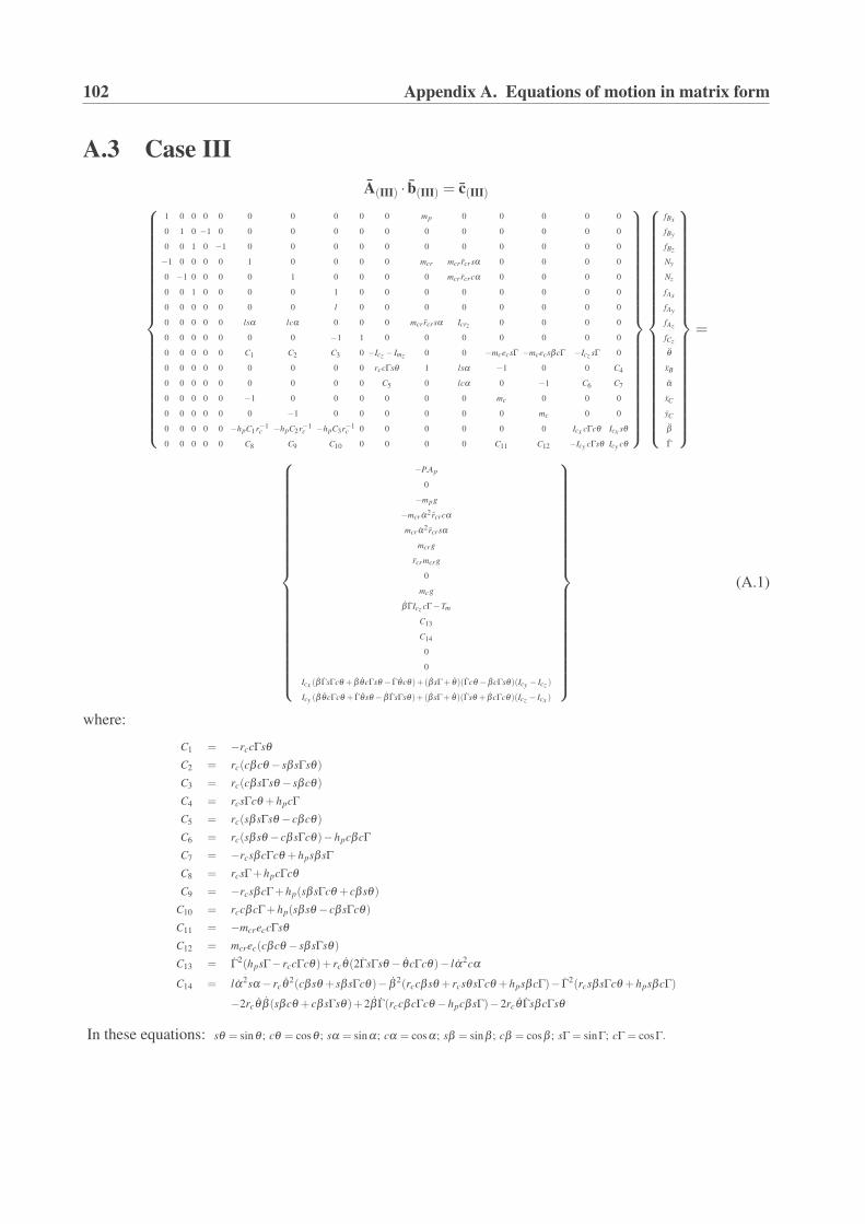
102 Appendix A. Equations of motion in matrix form
A.3 Case IIIA(III) · b(III) = c(III)⎧⎪⎪⎪⎪⎪⎪⎪⎪⎪⎪⎪⎪⎪⎪⎪⎪⎪⎪⎪⎨
⎪⎪⎪⎪⎪⎪⎪⎪⎪⎪⎪⎪⎪⎪⎪⎪⎪⎪⎪⎩
1 0 0 0 0 0 0 0 0 0 mp 0 0 0 0 0
0 1 0 −1 0 0 0 0 0 0 0 0 0 0 0 0
0 0 1 0 −1 0 0 0 0 0 0 0 0 0 0 0
−1 0 0 0 0 1 0 0 0 0 mcr mcr rcrsα 0 0 0 0
0 −1 0 0 0 0 1 0 0 0 0 mcr rcrcα 0 0 0 0
0 0 1 0 0 0 0 1 0 0 0 0 0 0 0 0
0 0 0 0 0 0 0 l 0 0 0 0 0 0 0 0
0 0 0 0 0 lsα lcα 0 0 0 mcr rcrsα Icrz 0 0 0 0
0 0 0 0 0 0 0 −1 1 0 0 0 0 0 0 0
0 0 0 0 0 C1 C2 C3 0 −Icz − Imz 0 0 −mcecsΓ −mcecsβcΓ −Icz sΓ 0
0 0 0 0 0 0 0 0 0 rccΓsθ 1 lsα −1 0 0 C4
0 0 0 0 0 0 0 0 0 C5 0 lcα 0 −1 C6 C7
0 0 0 0 0 −1 0 0 0 0 0 0 mc 0 0 0
0 0 0 0 0 0 −1 0 0 0 0 0 0 mc 0 0
0 0 0 0 0 −hpC1r−1c −hpC2r−1
c −hpC3r−1c 0 0 0 0 0 0 Icx cΓcθ Icx sθ
0 0 0 0 0 C8 C9 C10 0 0 0 0 C11 C12 −Icy cΓsθ Icy cθ
⎫⎪⎪⎪⎪⎪⎪⎪⎪⎪⎪⎪⎪⎪⎪⎪⎪⎪⎪⎪⎬⎪⎪⎪⎪⎪⎪⎪⎪⎪⎪⎪⎪⎪⎪⎪⎪⎪⎪⎪⎭
⎧⎪⎪⎪⎪⎪⎪⎪⎪⎪⎪⎪⎪⎪⎪⎪⎪⎪⎪⎪⎨⎪⎪⎪⎪⎪⎪⎪⎪⎪⎪⎪⎪⎪⎪⎪⎪⎪⎪⎪⎩
fBx
fBy
fBz
Ny
Nz
fAx
fAy
fAz
fCz
θ
xB
α
xC
yC
β
Γ
⎫⎪⎪⎪⎪⎪⎪⎪⎪⎪⎪⎪⎪⎪⎪⎪⎪⎪⎪⎪⎬⎪⎪⎪⎪⎪⎪⎪⎪⎪⎪⎪⎪⎪⎪⎪⎪⎪⎪⎪⎭
=
⎧⎪⎪⎪⎪⎪⎪⎪⎪⎪⎪⎪⎪⎪⎪⎪⎪⎪⎪⎪⎨⎪⎪⎪⎪⎪⎪⎪⎪⎪⎪⎪⎪⎪⎪⎪⎪⎪⎪⎪⎩
−P.Ap
0
−mpg
−mcr α2 rcrcα
mcr α2 rcrsα
mcrg
rcrmcrg
0
mcg
β ΓIcz cΓ−Tm
C13
C14
0
0
Icx (β ΓsΓcθ + β θcΓsθ − Γθcθ)+(β sΓ+ θ)(Γcθ − βcΓsθ)(Icy − Icz )
Icy (β θcΓcθ + Γθsθ − β ΓsΓsθ)+(β sΓ+ θ)(Γsθ + βcΓcθ)(Icz − Icx )
⎫⎪⎪⎪⎪⎪⎪⎪⎪⎪⎪⎪⎪⎪⎪⎪⎪⎪⎪⎪⎬⎪⎪⎪⎪⎪⎪⎪⎪⎪⎪⎪⎪⎪⎪⎪⎪⎪⎪⎪⎭
(A.1)
where:
C1 = −rccΓsθC2 = rc(cβcθ − sβ sΓsθ)C3 = rc(cβ sΓsθ − sβcθ)C4 = rcsΓcθ +hpcΓC5 = rc(sβ sΓsθ − cβcθ)C6 = rc(sβ sθ − cβ sΓcθ)−hpcβcΓC7 = −rcsβcΓcθ +hpsβ sΓC8 = rcsΓ+hpcΓcθC9 = −rcsβcΓ+hp(sβ sΓcθ + cβ sθ)
C10 = rccβcΓ+hp(sβ sθ − cβ sΓcθ)C11 = −mcreccΓsθC12 = mcrec(cβcθ − sβ sΓsθ)C13 = Γ2(hpsΓ− rccΓcθ)+ rcθ(2ΓsΓsθ − θcΓcθ)− lα2cα
C14 = lα2sα − rcθ 2(cβ sθ + sβ sΓcθ)− β 2(rccβ sθ + rcsθsΓcθ +hpsβcΓ)− Γ2(rcsβ sΓcθ +hpsβcΓ)
−2rcθ β (sβcθ + cβ sΓsθ)+2β Γ(rccβcΓcθ −hpcβ sΓ)−2rcθ ΓsβcΓsθ
In these equations: sθ = sinθ ; cθ = cosθ ; sα = sinα; cα = cosα; sβ = sinβ ; cβ = cosβ ; sΓ = sinΓ; cΓ = cosΓ.

Appendix B
Journal papersB.1 [J1] - International Journal of Mechanics, Vol.1 (4), 2007,
pp. 36-43.
103

�Abstract—A multibody dynamic model of the main mechanical components of a hermetic reciprocating compressor is presented in this work. The dynamics of the mechanical components are described with help of Dynamics of Multibody Systems (rigid components) and Finite Element Method (flexible components). Some of the mechanical elements are supported by fluid film bearings where the hydrodynamics interaction forces are described by the modified Reynolds equation. The system of nonlinear equations is numerically solved, taking into account the lateral and tilting vibration of the center of the crank. Particularly, in this study the main focus is on the lubrication behavior of the upper and lower bearings of the crankshaft, considering hydrodynamic lubrication conditions. The behavior of the orbits and the pressure distribution in the journal bearings is presented giving some insights into design parameters, such as, maximal fluid film pressure, minimum fluid film thickness and maximum vibration levels.
Keywords— Multibody dynamics, hydrodynamic lubrication, journal bearings, hermetic compressor.
I. INTRODUCTION
mall-scale hermetic reciprocating compressors are widely used to compress coolant gas in household
refrigerators and air-conditioners. Almost since the 60's these small machines became a necessary appliance in every household in the industrialized countries. Since then, a lot of research has been done to optimize the design and to improve the thermal and mechanical efficiency. Hermetic reciprocating compressors use pistons that are driven directly through a slider-crank mechanism, converting the rotating movement of the rotor to an oscillating motion. In this type of compressors, motor and compressor are directly coupled on the same shaft and the assembly is installed inside a welded steel shell. A
Manuscript received April 29, 2007: Revised version received Octob. 3,2007. The authors gratefully acknowledge the support given by the Programme Al�an, the European Union Programme of High Level Scholarships for Latin America, scholarship No. E06D101992CO.
Edgar A. Estupiñan (corresponding author) is with the Mechanical Engineering Department, Technical University of Denmark, Kgs. Lyngby, DK 2800 Denmark. (phone: +45- 4525-5678; fax: +45-4593-1475; e-mail: [email protected]).
Ilmar F. Santos, is Associate Professor of the Mechanical Engineering Department, Technical University of Denmark, Kgs. Lyngby, DK 2800 Denmark. (e-mail: [email protected]).
schematic view of a hermetic reciprocating compressor used in household refrigerators is shown in Fig. 1.
Fig. 1. Hermetic reciprocating compressor
The study and optimization of the dynamic behavior of reciprocating compressors, taking in account the hydrodynamics of bearings is of significant importance for the development of new prototypes. The performance of the bearings affects key functions such as durability, noise and vibration of the compressor. Optimization of the behavior of journal bearings by means of numerical simulation may reduce development costs for prototype testing work significantly.
Several computational models for the analysis of small reciprocating compressors can be found in the literature. They range from simple simulations including steady-state energy balance until more complex models of unsteady analysis of the heat and work transfer and thermal and fluid dynamic analysis. A complete literature review of previous studies with focus on compressor simulation models is included in [1]. Some of these studies require numerical simulations of the refrigerant flow through the valves and inside the cylinder during the compression cycle [2], whereas other studies focus mainly on the dynamics of motion in steady and transient conditions [3]. For instance, a study that included the coupling of fluid-structure dynamics to analyze the dynamics of piston is presented in [4]. Reference [5] shows an analytical model of the coupled dynamic behavior of the piston and crankshaft, with comparisons between a finite bearing model and a short
Dynamic Modeling of Hermetic Reciprocating Compressors, Combining Multibody Dynamics,
Finite Elements Method and Fluid Film Lubrication
Edgar A. Estupiñan and Ilmar F. Santos
S
INTERNATIONAL JOURNAL OF MECHANICS
Issue 4, Volume 1, 2007 36
104 Appendix B. Journal papers

bearing approach. In the same study, a numerical procedure combining Newton-Raphson method and the successive over relaxation scheme to solve the equations was presented. In the study carried out by Cho and Moon [4], a time-incremental numerical algorithm to solve a finite differences model for the estimation of the oil film pressure is coupled with a finite element model for the computation of the structural deformation of the piston.
Although most of the work done related to modeling of compressors is related to the thermal and fluid dynamic behavior, in this work the main focus and contribution are on the developing of a multibody dynamic model that represents the dynamics of the main mechanical components of hermetic compressors. This model is coupled with a finite element model of the rotor, where the hydrodynamic interaction forces are computed using analytical solutions of Reynolds equation. The elastohydrodynamic theory, which takes into account the bearing and housing flexibility, is not considered in this paper, since it is presented only in very special cases.
II. MATHEMATICAL MODELING
In this section the formulation of representative equations describing the mathematical simulation model for a hermetic compressor is developed. The motion of the piston has been modeled as particle, the motion of the connecting rod and crank as rigid bodies and the shaft is modeled as a flexible body via finite elements. The motion equations for the piston connecting-rod crank system are formulated using the Newton-Euler's method. Fig. 2 shows a sketch indicating the inertial referential frame system XYZ and the main angles of rotation for the moving reference frames.
Fig. 2. Piston – connecting rod – crank system. Geometry and reference frames
A. Reference Frames One inertial reference frame (IXYZ) and four moving
reference frames (B1, B2, B3 and B4) have been defined. The reference frames B1, B2 and B3 are attached to the crank to describe the tilting and rotational movement of the crank and the reference frame B4 is attached to the connecting rod. B1
(X1Y1Z1) is obtained by rotating I the angle � around X axis;
B2 (X2Y2Z2), is obtained by rotating B1 the angle � around Y1
axis; B3 (X3Y3Z3), is obtained by rotating B2 the angle �around Z2 axis and B4 (X4Y4Z4), is obtained by rotating I the angle � around Z axis.
B. Constraint Equations A constraint equation that takes into account lateral
displacements and tilting oscillations of the center of the crank is given in (1). A simplified sketch illustrating how the basic elements of the system are connected is shown in Figure 2b.
CRLX IIIpI �� (1)
where: RTTTR3B
TTTI ��� � �� ; � �T0
3 pcB hr �R
C. Kinematics The absolute angular velocity (�) written with help of B3, is
given by:
���� ���3333 BBBB �� �� (2)
where: �� ��IB ��� � �� TTT
3 ; �� ��
13 BB �� �TT� ; �� ��
23 BB � �T
The velocities and accelerations of the piston ( Bx� , Bx�� ) and the connecting rod (�� ,��� ), are obtaining when the constraint equation (1) is differentiated once and twice respectively, obtaining:
���
���
���
����
� �
�
2
1
cos0sin1
vvx
ll B
���
�
� (3)
���
���
���
����
� �
�
2
1
cos0sin1
aax
ll B
���
��
�� (4)
where, the variables 1v , 2v , 1a , 2a are giving in appendix (A).
D. Equations of Motion The equations of motion are formulated using Newton-
Euler's method [6]. The equations of motion for each body are given in Table I.
The equations of motion for the multibody dynamic model may be written in a matrix form as in (10), where vector fcontains the unknown variables such as: reaction forces, reaction moments and accelerations of the system. This matrix system will be coupled to the equations from the finite element formulation of the crankshaft, which is explained later in section IV.
cfA � (10)
INTERNATIONAL JOURNAL OF MECHANICS
Issue 4, Volume 1, 2007 37
B.1 [J1] - International Journal of Mechanics, Vol.1 (4), 2007, pp. 36-43. 105

TABLE IEQUATIONS OF MOTION
Body Force Equation Moment Equation
Crank � �T, CCcAIcIcI yxmm ������ FaF (5) mBABBOB TFrM3333
��� (6)
� � � � OBcmCBcBOBBBOB mdtd ar�I��I
3333333������ �
where: AIAB FTTTF ��� � ��3 ; � �T,0,0
3 zmB TT ;
� �T0,0,3 ccmCB e�r
Connecting
rodBIAIcrIcrI m FFaF ���
(7)where:
� �� �
��
��
�
��
��
�
���
�����
0sincos
sincos2
2
��������
���
�����
����
cr
crB
crIIcrIIIBIcrI
rrx
r�r��aa
ABBBB FlM444
�� (8)
� � � � BBcrBcrBcrBBBcrB mdtd ar�I��I
4444444������� ���
where: AIAB FTF �4
; BIBB aTa �4
; � �T0,0,BBI x��a
Piston pIIBIBIpBI m FNFaF ���� (9)
where: � �T0,0,pgpI AP �F
where:
� �T4321 ,,,,,,,,,,,,,,, qqqqxffffNNfff BCAAAzyBBB zzyxzyx�������������� ��f
and 1q�� , 2q�� , 3q�� , 4q�� , correspond to the angular accelerations of the crank center.
A. Modeling of the Rotor The main rotor-shaft of the compressor, which drives the
crank-connecting rod-piston system, is modeled as a flexible body via finite elements method [7]. The global equation of motion described in the inertial reference frame is given by:
�� ��� �����
f
qKqDFqM ... �� (11)
where F , is the vector that includes the external forces on the rotor such as: preload forces, rotor unbalance forces and the fluid film bearing forces.
III. FLUID FILM FORCES
The main geometrical relations of a journal bearing are shown in Fig. 3. The governing equation for the pressure distribution of the oil film in dynamically loaded journal bearings may be obtained from the general formulation of Reynolds’ equation [8]. The modified Reynolds equation for dynamically loaded journal bearings is given by (12), where,
�� is the rotational speed of the journal center about the bearing center and is the relative eccentricity. The fluid film thickness may be calculated using: )cos1( ! � bb ch , where
! is the angle measured from the location of the maximum film thickness.
�
� �
�"#$
%&' (
�))
�))
""#
$%%&
'))
))
�""#
$%%&
'))
))
2sincos12 2
32
3
ttrc
zph
zrph
bbb
bb �! !
*!*!(12)
Fig. 3. Journal bearing geometry
With dynamically loaded bearings the eccentricity and attitude angle will vary through the loading cycle. The pressure generated when a journal bearing is dynamically loaded can be determined if the normal squeeze velocity ( � )and the rotational velocities ( (,�� ) are known at any eccentricity ratio. Complete solutions of (12) may be obtained
INTERNATIONAL JOURNAL OF MECHANICS
Issue 4, Volume 1, 2007 38
106 Appendix B. Journal papers

numerically, and solutions for limited cases may be also obtained analytically. In this work analytical solutions for the short-width bearing and infinitely-long-width bearing theories have been used. The short-journal-bearing theory assumes that the variation of pressure is more significant in the axial direction than in the circumferential direction and therefore the first term in (12) can be neglected. In contrast, for an infinitely long-width-journal-bearing, the pressure in the axial direction is assumed to be constant, therefore, in this case, the side-leakage term, i.e., the second term in (12), can be neglected. For each one of these two particular cases, the fluid film pressure distribution can be easily computed, analytically integrating the Reynolds equation and similarly, the journal bearing forces in + ,, coordinates can be calculated, integrating the pressure distribution analytically obtained. If the pressure is integrated over all the fluid film around the bearing (i.e, -! 20 .. ), this solution is known as a full Sommerfeld solution. However, if the analysis is limited to the convergent film (i.e., -! ..0 ), this is known as a half Sommerfeld solution. The analytical expressions used in this paper for the computation of the radial and transversal fluid film forces (F+, F,), for a long and a short journal bearing, are giving in [9].
IV. NUMERICAL SOLUTION
The equation of motions for each connected body of the multibody system together with the FEM model of the shaft and the analytical expressions for the fluid film forces yield to a system of high complexity and non-linearity. The numerical algorithm implemented is shown in Fig. 4. Considering that the system has a "stiff" behavior because of the combination of a rigid body model with a finite element model, a Newmark implicit method combined with a predictor-corrector approach [10], is used in this work. The simulation procedure is summarized in the following main steps:
Input data and starting values. In this part the geometrical and physical parameters must be given, such as, physical dimensions, rotational speed, masses, inertias, preloads, initial displacements and initial velocities.
Pre-processing. This part includes the generation of structural matrices for the multibody model (MBD module) and the matrices of the flexible rotor (FEM module). Based on the initial conditions, initial fluid film forces are computed using the FFF module.
Numerical computation. This part includes the coupling of matrices, the computation of the journal bearing forces at each time step and the numerical solution of the global system. At each time step, new fluid film forces are computed and included in the global matrix system (13) where the equilibrium has to be achieved. In (13), the matrix M is
formed by the matrix M of size ndofndof � , coupled to the matrix A of size 1616� in the degrees of freedom related to the linear and angular accelerations of the crank center node ( 1q�� , 2q�� , 3q�� , 4q�� ). Thus, the final size of the global mass matrix
( M ) is 12�ndof . Similarly, in (13) the global right hand side vector, Q , is formed by coupling the resultant right hand side vector, f , in (11), to the vector c , in (10). The iterative equations to solve the global system (13), by using the Newmark implicit method, are given by (14)-(16).
� � QqfM ˆ,ˆˆ T� �� (13)
where:
� �T,,,,,,,,,,,ˆ �� ������ BCAAAzyBBB xffffNNfff
zzyxzyxf and
� �T21 ,...,, ndofqqq �������� q .
� �1111
ˆˆ,ˆ 1T
����� �
iiii tttt QMqf �� (14)
/ � � 011
ˆˆ1��
���iiii tttt qqhqq ������ 11 (15)
/ � � 011
ˆ2ˆ212
2
������
iiiii ttttt qqhqhqq ����� �� (16)
INTERNATIONAL JOURNAL OF MECHANICS
Issue 4, Volume 1, 2007 39
B.1 [J1] - International Journal of Mechanics, Vol.1 (4), 2007, pp. 36-43. 107

Fig. 4. Flowchart of the numerical computer code
To compute1�it
q�� , the load vector 1
ˆ�it
Q must be estimated
previously, which implies to calculate the vector of journal bearing forces
1�itb Q , which depends on the positions and
velocities at the time 1�it . Therefore, initial values for 01�it
q� and0
1�itq are predicted by using the Heun's explicit method. Then,
11�it
q�� can be initially estimated by using (14) and then, 11�it
q� and1
1�itq can be calculated using (15) and (16) respectively. With
these new estimated values, the journal bearing forces are updated and using again (14) a new estimation of 2
1�itq�� can be
obtained, and so on until the difference of two consecutive values is smaller than the prescribed tolerance given. Additionally, by using the explicit Euler method, the crank angle
it� and the instantaneous angular velocity
it�� are
estimated at each time step.
Post-processing. This part includes the generation of plots of journal bearing orbits, journal bearing forces, maximum oil film pressure, minimum fluid film thickness and reaction forces as a function of the instantaneous crank angle.
V. NUMERICAL RESULTS
The main geometrical dimensions and physical properties of the reciprocating compressor used for the numerical simulations are given in Table II. The curve of gas pressure (Pg) as function of the crank angle, used for the simulations in this work, is giving in [4] and is shown in Fig. 5. An experimental curve of motor torque for a typical motor of a hermetic compressor is taken from [1] and shown in Fig. 6.
The following results were obtained, using a computer code implemented according to the flow chart of Fig. 4 and using a time step of 61 �2 et s to warranty the convergence of the solution.
TABLE II.MAIN GEOMETRICAL AND PHYSICAL PARAMETERS
Radius crank-pin center rc = 7.5 mmRadius of bearings rb = 8 mmWidth of bearings lb = 6 mmJournal clearance cb = 15 *m
Length of crank pin hp = 10 mmDistance between
bearings L = 80 mm
Moments of inertia of motor-rotor
Ix, Iy = 0.4x10⁻³ kg.m2,Iz = 0.1x10⁻² kg.m2
Diameter of piston Dp = 23 mm (Ap = 415.5 mm2)Mass of the piston mp = 0.043 kgLubricant viscosity * = 0.005 Pa.sAngular velocity ( = 312 rad/s (2980 rpm)Crank unbalance mub = 0.05 kg, rub = 5 mm
0 45 90 135 180 225 270 315 3600
2
4
6
8
10
Crankshaft angle [deg]
Gas
pre
ssur
e [P
a x
105 ]
Figure 5. Curve of the gas pressure (Pg) as a function of the crankshaft angle
2500 2600 2700 2800 2900 30000
0.5
1
1.5
Angular velocity [rpm]
Torq
ue [N
.m]
Fig. 6. Curve of the motor torque (Tm) as a function of the angular velocity.
Fig. 7 shows the journal bearing forces for the upper and
INTERNATIONAL JOURNAL OF MECHANICS
Issue 4, Volume 1, 2007 40
108 Appendix B. Journal papers
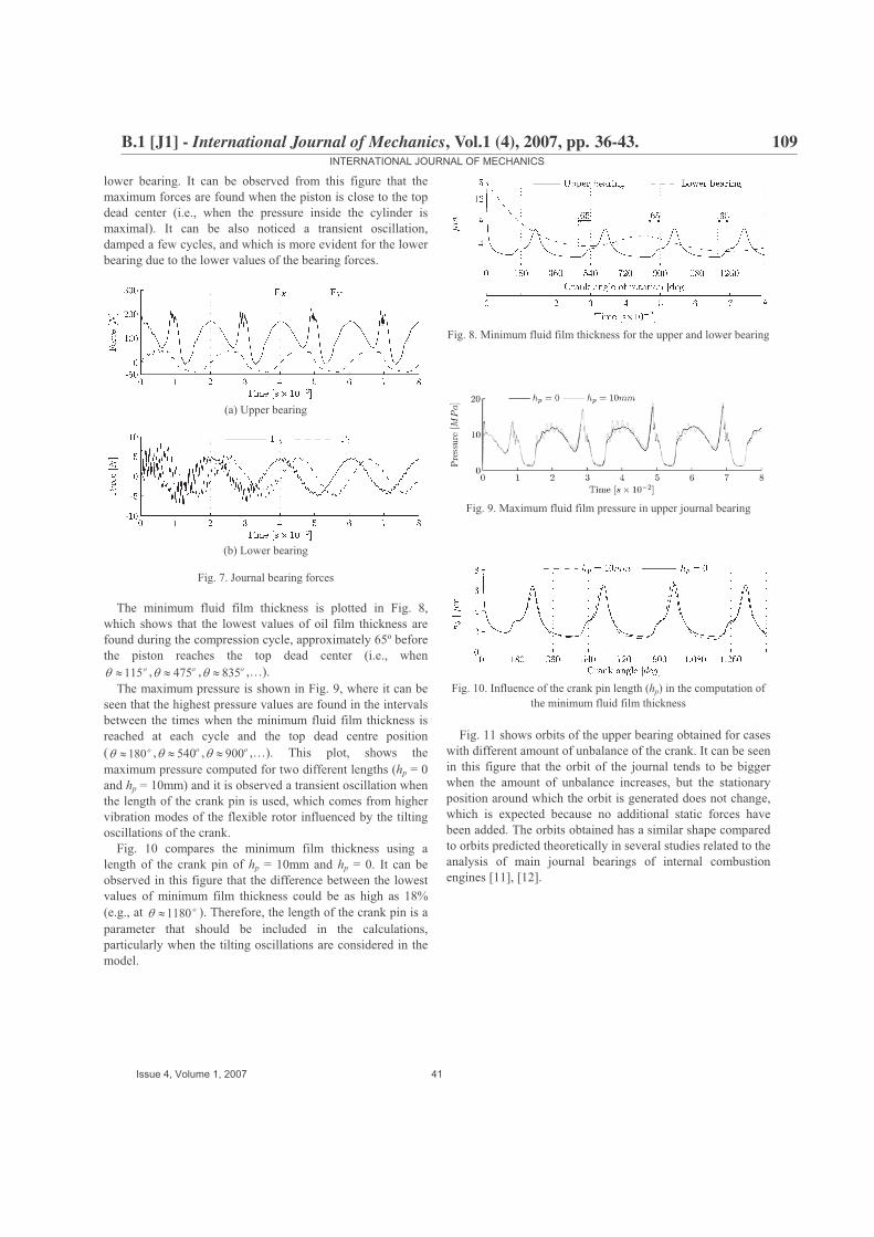
lower bearing. It can be observed from this figure that the maximum forces are found when the piston is close to the top dead center (i.e., when the pressure inside the cylinder is maximal). It can be also noticed a transient oscillation, damped a few cycles, and which is more evident for the lower bearing due to the lower values of the bearing forces.
(a) Upper bearing
(b) Lower bearing
Fig. 7. Journal bearing forces
The minimum fluid film thickness is plotted in Fig. 8, which shows that the lowest values of oil film thickness are found during the compression cycle, approximately 65º before the piston reaches the top dead center (i.e., when
o1153� , o4753� , o8353� ,…).The maximum pressure is shown in Fig. 9, where it can be
seen that the highest pressure values are found in the intervals between the times when the minimum fluid film thickness is reached at each cycle and the top dead centre position ( o1803� , o5403� , o9003� ,…). This plot, shows the maximum pressure computed for two different lengths (hp = 0 and hp = 10mm) and it is observed a transient oscillation when the length of the crank pin is used, which comes from higher vibration modes of the flexible rotor influenced by the tilting oscillations of the crank.
Fig. 10 compares the minimum film thickness using a length of the crank pin of hp = 10mm and hp = 0. It can be observed in this figure that the difference between the lowest values of minimum film thickness could be as high as 18% (e.g., at o11803� ). Therefore, the length of the crank pin is a parameter that should be included in the calculations, particularly when the tilting oscillations are considered in the model.
Fig. 8. Minimum fluid film thickness for the upper and lower bearing
Fig. 9. Maximum fluid film pressure in upper journal bearing
Fig. 10. Influence of the crank pin length (hp) in the computation of the minimum fluid film thickness
Fig. 11 shows orbits of the upper bearing obtained for cases with different amount of unbalance of the crank. It can be seen in this figure that the orbit of the journal tends to be bigger when the amount of unbalance increases, but the stationary position around which the orbit is generated does not change, which is expected because no additional static forces have been added. The orbits obtained has a similar shape compared to orbits predicted theoretically in several studies related to the analysis of main journal bearings of internal combustion engines [11], [12].
INTERNATIONAL JOURNAL OF MECHANICS
Issue 4, Volume 1, 2007 41
B.1 [J1] - International Journal of Mechanics, Vol.1 (4), 2007, pp. 36-43. 109
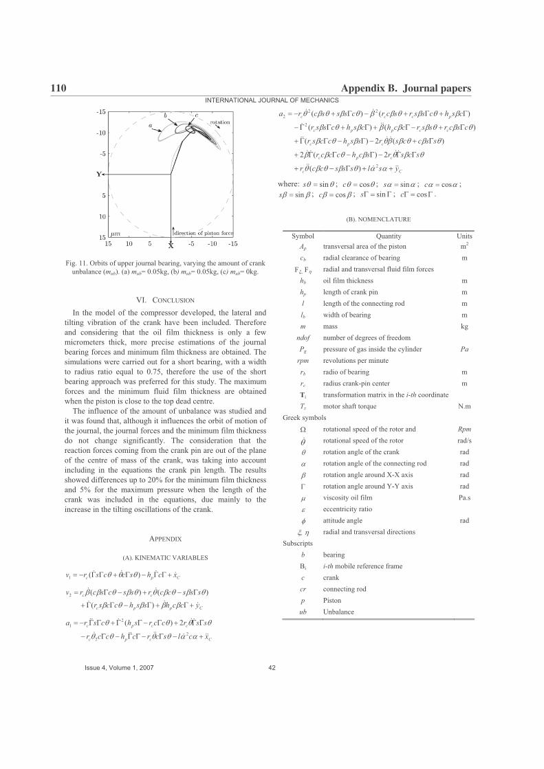
Fig. 11. Orbits of upper journal bearing, varying the amount of crank unbalance (mub). (a) mub= 0.05kg, (b) mub= 0.05kg, (c) mub= 0kg.
VI. CONCLUSION
In the model of the compressor developed, the lateral and tilting vibration of the crank have been included. Therefore and considering that the oil film thickness is only a few micrometers thick, more precise estimations of the journal bearing forces and minimum film thickness are obtained. The simulations were carried out for a short bearing, with a width to radius ratio equal to 0.75, therefore the use of the short bearing approach was preferred for this study. The maximum forces and the minimum fluid film thickness are obtained when the piston is close to the top dead centre.
The influence of the amount of unbalance was studied and it was found that, although it influences the orbit of motion of the journal, the journal forces and the minimum film thickness do not change significantly. The consideration that the reaction forces coming from the crank pin are out of the plane of the centre of mass of the crank, was taking into account including in the equations the crank pin length. The results showed differences up to 20% for the minimum film thickness and 5% for the maximum pressure when the length of the crank was included in the equations, due mainly to the increase in the tilting oscillations of the crank.
APPENDIX
(A). KINEMATIC VARIABLES
Cpc xchsccsrv ���� ��������� )(1 ���
Cppc
cc
ycchsshccsr
sssccrsscscrv���
��
��������
�����
�����
����������
)(
)()(2
Ccpc
ccpc
xclscrchccr
ssrccrshcsra
��������
�����
���������
�����������
������
����2
2
21 2)(
Cc
cpc
cpc
ccppc
pccc
yslsssccr
scsrschcccr
ssccsrsshccsr
cscrssrcchcshcssr
cshcssrscrcssscra
�����
����
����
���
��
�����
��������
��������
����������
��������
�������
�������
���������
���������
�����������
2
2
222
)(
2)(2
)(2)(
)()(
)()(
where: �� sins ; �� cosc ; �� sins ; �� cosc ;�� sins ; �� cosc ; �� sins ; �� cosc .
(B). NOMENCLATURE
Symbol Quantity UnitsAp transversal area of the piston m2
cb radial clearance of bearing m
F+,, F, radial and transversal fluid film forces hb oil film thickness m hp length of crank pin m l length of the connecting rod m lb width of bearing m m mass kg
ndof number of degrees of freedom Pg pressure of gas inside the cylinder Pa
rpm revolutions per minute rb radio of bearing m rc radius crank-pin center m Ti transformation matrix in the i-th coordinate Tz motor shaft torque N.m
Greek symbols
( rotational speed of the rotor and Rpm
�� rotational speed of the rotor rad/s
� rotation angle of the crank rad
� rotation angle of the connecting rod rad
� rotation angle around X-X axis rad
� rotation angle around Y-Y axis rad
* viscosity oil film Pa.s
eccentricity ratio
� attitude angle rad
+, , radial and transversal directions Subscripts
b bearingBi i-th mobile reference frame c crankcr connecting rod p Piston
ub Unbalance
INTERNATIONAL JOURNAL OF MECHANICS
Issue 4, Volume 1, 2007 42
110 Appendix B. Journal papers

REFERENCES
[1] J. Rigola, “Numerical simulation and experimental validation of hermetic reciprocating compressors”, PhD dissertation, Universidad Politécnica de Cataluña, Barcelona, Spain, 2002.
[2] G. Longo and A. Gasparella, “Unsteady state analysis of the compression cycle of a hermetic reciprocating compressor”, International Journal of Refrigeration, vol. 26, no. 6, pp. 681-689, 2003.
[3] R. Dufour, J. Der Hagopian and M. Lalanne, “Transient and steady state dynamic behaviour of single cylinder compressors: Prediction and experiments”, Journal of Sound and Vibration, vol. 181, no. 1, pp. 23-41, 1995.
[4] J. R. Cho and S. J. Moon, “A numerical analysis of the interaction between the piston oil film and the component deformation in a reciprocating compressor”, Tribology International, vol. 38 no. 5, pp. 459-468, 2005.
[5] T. J. Kim and J. S. Han, “Comparison of the dynamic behavior and lubrication characteristics of a reciprocating compressor crankshaft in both finite and short bearing models”, Tribology Transactions, vol. 47, no. 1, pp. 61-69, 2004.
[6] I. F. Santos, Dinâmica de Sistemas Mecanicos, (in Portuguese). Makron Books, Sao Paulo, Brazil, 2001.
[7] H. D. Nelson, , “A finite rotating shaft element using Timoshenko beam theory”, Journal of Mechanical Design, Transactions of the ASME, vol. 102, no. 4, pp. 793-803, 1980.
[8] B. J. Hamrock, Fundamental of Fluid Film Lubrication, NASA Reference Publication, USA, 1991.
[9] J. Frêne, D. Nicolas, B. Degueurce, D. Berthe and M. Godet, Lubrification Hydrodynamique, Editions Eyrolles, Paris, 1990.
[10] J. Garcia de Jalon and E. Bayo, Kinematic and Dynamic Simulation of Multibody Systems. The Real-Time Challenge, Springer-Verlag, New-York, 1994.
[11] R. Pal, R. Sinhasan and D. Singh, “Analysis of a big-end bearing - a finite element approach”, Wear, vol. 121, no. 1, pp. 117-120, 1988.
[12] G. S. Ritchie, “The prediction of journal loci in dynamically loaded internal combustion engine bearings”, Wear, vol. 35, no. 2, pp. 291-297, 1975.
INTERNATIONAL JOURNAL OF MECHANICS
Issue 4, Volume 1, 2007 43
B.1 [J1] - International Journal of Mechanics, Vol.1 (4), 2007, pp. 36-43. 111

112 Appendix B. Journal papers
B.2 [J2] - Journal of the Brazilian Society of Mechanical Sci-ences and Engineering, Vol.31 (1), 2009, pp. 35-46.

Modelling Hermetic Compressors Using Different Constraint Equations to …
J. of the Braz. Soc. of Mech. Sci. & Eng. Copyright 4 2009 by ABCM January-March 2009, Vol. XXXI, No. 1 / 35
Edgar A. Estupiñan [email protected]
Ilmar F. Santos Senior Member, ABCM
[email protected] Technical University of Denmark
Department of Mechanical Engineering Nils Koppels Allé, Building 404, DK-2800
Kgs. Lyngby, Denmark
Modelling Hermetic Compressors Using Different Constraint Equations to Accommodate Multibody Dynamics and Hydrodynamic Lubrication In this work, the steps involved for the modelling of a reciprocating linear compressor are described in detail. The dynamics of the mechanical components are described with the help of multibody dynamics (rigid components) and finite elements method (flexible components). Some of the mechanical elements are supported by fluid film bearings, where the hydrodynamic interaction forces are described by the Reynolds equation. The system of nonlinear equations is numerically solved for three different restrictive conditions of the motion of the crank, where the third case takes into account lateral and tilting oscillations of the extremity of the crankshaft. The numerical results of the behaviour of the journal bearings for each case are presented giving some insights into design parameters such as, maximum oil film pressure, minimum oil film thickness, maximum vibration levels and dynamic reaction forces among machine components, looking for the optimization and application of active lubrication towards vibration reduction. Keywords: hermetic compressor, multibody dynamics, journal bearing, Reynolds equation, hydrodynamic lubrication.
Introduction 1One of the most common types of compressors used in the
refrigeration field is the piston compressor, also known as reciprocating compressor. Small-scale hermetic reciprocating compressors are widely used to compress coolant gas in household refrigerators and air-conditioners. It was at the beginning of the Sixties when these small machines became a household appliance of common use in the industrialized countries. Since then, numerous research studies have been carried out in order to optimize the design and to improve the thermal and mechanical efficiency of refrigeration compressors. Positive displacement compressors mechanically drive the refrigerant gas from the evaporator at low-pressure side to the condenser at high-pressure side, reducing the compressor chamber volume. Reciprocating compressors use pistons that are driven directly through a slider-crank mechanism, converting the rotating movement of the rotor to an oscillating motion. A hermetic reciprocating compressor is a particular case where motor and compressor are directly coupled on the same shaft and contained within the same housing (welded steel shell) and in contact with the refrigerant and oil (Rigola, 2002). A picture and a schematic draw of a hermetic reciprocating compressor used in household refrigerators are shown in Fig.1.
Figure 1. Picture and schematic draw of a hermetic reciprocating compressor.
Paper accepted December, 2008. Technical Editor: Domingos A. Rade.
The study and optimization of the dynamic behaviour of reciprocating compressors, taking in account the hydrodynamics of bearings, are of significant importance for the development of new prototypes. The performance of the bearings affects key functions such as durability and noise and vibration behaviour of the compressor. Optimization studies of the performance of journal bearings by means of numerical simulation may reduce development costs for prototype testing work significantly. Several studies that involve numerical studies and computational models for the analysis of small reciprocating compressors are found in the literature, as it can be seen in the works carried out by Rasmussen (1997) and Rigola (2002). In some studies, numerical simulations of the refrigerant flow through the valves and inside the cylinder during the compression cycle have been included (Longo and Gasparella, 2003), whereas in others the focus has been on the dynamics of motion in steady and transient conditions (Dufour, et al., 1995). Some researchers have included the coupling of fluid-structure dynamics in order to particularly analyse the dynamics of the piston (Gommed and Etsion, 1993; Cho and Moon, 2005). In a study carried out by Kim and Han (2004), an analytical model of the coupled dynamic behaviour of the piston and crankshaft was developed and comparisons between a finite bearing model and a short bearing approach were included. In the same study, a numerical procedure that combines Newton-Raphson method and the successive over relaxation scheme was also presented. In the study carried out by Cho and Moon (2005), a time-incremental numerical algorithm to solve a finite differences model for the estimation of the oil film pressure was coupled with a finite element model for the computation of the structural deformation of the piston. As it is described here, many of the research studies related to compressor modelling are mainly focused on the study of the thermal and fluid dynamic behaviour. In contrast, the main focus of the present work is on the developing of a multibody dynamic model of a hermetic compressor, where the dynamics of the fluid film bearings and the flexibility of the crankshaft are included. The multibody dynamic model, which includes the main mechanical components of the hermetic compressor, is coupled with a finite elements model of the rotor and the hydrodynamic interaction forces, which are computed using analytical solutions of the Reynolds equation. The influence of the crankshaft tilting oscillations on design parameters, such as the minimum film
B.2 [J2] - Journal of the Brazilian Society of Mechanical Sciences and Engineering, Vol.31 (1),2009, pp. 35-46. 113
Edgar A. Estupiñan and Ilmar F. Santos
36 / Vol. XXXI, No. 1, January-March 2009 ABCM
thickness and maximum pressures are carefully investigated, since the finite element model allows capturing of such movements. The elasto-hydrodynamic theory, which takes in account the bearing and housing flexibility, is not considered in this work, since it is presented only in very special cases.
Nomenclature Ap =transversal area of the piston, m2 cb =radial clearance of the bearing, m Dp =piston diameter, m ec =mass eccentricity of the crank, m f =vector of forces, N fb =vector of journal bearing forces, N hb =oil film thickness, m hp =length of crank pin, m I =moment of inertia tensor l =length of the connecting rod, m lb =width of the bearing, m m =mass, kg ndof =number of degrees of freedom Pg =gas pressure inside the cylinder, Pa p =fluid film pressure, Pa rpm =revolutions per minute r =radius, m S =Sommerfeld number Ti =transformation matrix in the coordinate i xB =piston position along the X direction, m Greek Symbols ( =rotational speed of the crankshaft, rad/s � =rotation angle of the crank around Z-Z axis, rad � =rotation angle of the connecting rod, rad � =rotation angle around X-X axis, rad � =rotation angle around Y1-Y1 axis, rad * =viscosity oil film, Pa.s =eccentricity ratio � =attitude angle, rad 5z =motor shaft torque, Nm Subscripts A,B,C =relative to the points A, B or C, respectively b =relative to the bearing Bi =relative to the i-th mobile reference frame c =relative to the crank cr =relative to the connecting rod p =relative to the piston I =relative to the inertial reference frame N =relative to normal reaction forces cylinder-piston LJB =relative to infinitely long-width journal bearing SJB =relative to short-width journal bearing X,Y =relative to the X and Y directions +, , =relative to the radial and transversal directions
Mathematical Modelling In this section the formulation of representative motion
equations to describe the mathematical model of a hermetic reciprocating compressor is developed. The main components of the reciprocating mechanism (i.e., connecting rod and crank) are modelled as rigid bodies, the piston motion is modelled as a particle and the main shaft is modelled as a flexible body via finite elements.
Three different approaches which differ in the definition of the restrictive conditions of motion of the centre of the crank have been comparatively studied. These three cases are:
- Case (I). Neglecting lateral displacements and tilting oscillations of the crank (no hydrodynamic bearings).
- Case (II). Considering lateral displacements but not tilting oscillations of the crank (rigid crankshaft).
- Case (III). Considering lateral displacements and tilting oscillations of the crank (flexible crankshaft).
Although the two first approaches make the problem simpler and reduce the computational time, by including the tilting crank effect in the model (case III), a more precise estimation of the journal bearing forces and the journal orbits may be obtained, considering that the oil film thickness is usually only a few micrometers thick. In order to include the tilting oscillations of the crank, the crankshaft is modelled via finite elements and coupled to the motion equations of the piston-slider-crank mechanism through the degrees of freedom where the shaft is connected to the crank. Furthermore, the fluid film forces in the upper and lower bearings are calculated by using analytical solutions of the Reynolds equation, and introduced into the equations of the rotor at each time. Therefore, depending on the case of study, the dynamics of the compressor is described by a different global system of equations.
Developing of the Multibody Dynamics Model
The motion equations of the piston-connecting rod-crank system have been formulated using the Newton-Euler's method, following the methodology suggested by Santos (2001). Figure 2 shows a sketch indicating the inertial referential frame IXYZ and the main angles of rotation for the four moving reference frames.
(a) Definition of the Inertial and Moving Reference Systems.
One inertial reference frame IXYZ and four moving reference frames have been defined. The inertial reference frame is attached to the centre of the bearing (point O), whereas, the moving reference frames B1, B2 and B3 are attached to the crank, and the moving reference frame B4 is attached to the connecting rod. B1 (X1Y1Z1) is obtained by rotating I, the angle �, around the X axis; B2 (X2Y2Z2) is obtained by rotating B1, the angle �, around the Y1 axis; B3 (X3Y3Z3)is obtained by rotating B2, the angle �, around the Z2 axis, and B4(X4Y4Z4) is obtained by rotating I, the angle �, around the Z axis. The transformation matrices are given by:
T�: transformation from the inertial frame I to the moving frame B1.
�
�
�
�
�
�����
cossinsincos
00
001T
T�: transformation from the inertial frame B1 to the moving frame B2.
�
�
�
� �
��
��
�cossin
sincos
0010
0T
T�: transformation from the inertial frame B2 to the moving frame B3.
�
�
�
��
10000
����
� cossinsincos
T
T�: transformation from the inertial frame I to the moving frame B4.
�
�
�
� �
10000
����
� cossinsincos
T
114 Appendix B. Journal papers
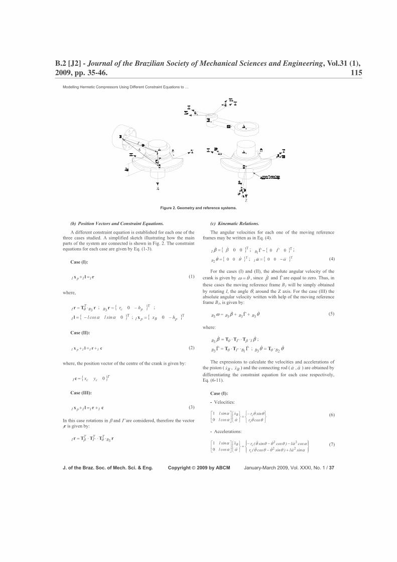
Modelling Hermetic Compressors Using Different Constraint Equations to …
J. of the Braz. Soc. of Mech. Sci. & Eng. Copyright 4 2009 by ABCM January-March 2009, Vol. XXXI, No. 1 / 37
Figure 2. Geometry and reference systems.
(b) Position Vectors and Constraint Equations.
A different constraint equation is established for each one of the three cases studied. A simplified sketch illustrating how the main parts of the system are connected is shown in Fig. 2. The constraint equations for each case are given by Eq. (1-3).
Case (I):
rlx IIpI � (1)
where,
rTr 3BT
I � � ; � �TpcB hr � 03 r ;
� �T0�� sinlcoslI �l ; � �TpBpI hx � 0x
Case (II):
crlx IIIpI �� (2)
where, the position vector of the centre of the crank is given by:
� �TccI yx 0c
Case (III):
crlx IIIpI �� (3)
In this case rotations in � and � are considered, therefore the vector Ir is given by:
rTTTr 3BTTT
I ��� ���
(c) Kinematic Relations.
The angular velocities for each one of the moving reference frames may be written as in Eq. (4).
� �T00��� �I ; � �T001 ��� �B ;
� �T��� 002 �B ; � �T��� � 00�I (4)
For the cases (I) and (II), the absolute angular velocity of the crank is given by �� � , since �� and �� are equal to zero. Thus, in these cases the moving reference frame B3 will be simply obtained by rotating I, the angle �, around the Z axis. For the case (III) the absolute angular velocity written with help of the moving reference frame B3, is given by:
���� ���3333 BBBB �� �� (5)
where:
�� ��IB ��� ��� TTT3 ;
�� ��13 BB �� �� TT ; �� ��
23 BB � �T
The expressions to calculate the velocities and accelerations of the piston ( Bx� , Bx�� ) and the connecting rod (�� ,��� ) are obtained by differentiating the constraint equation for each case respectively, Eq. (6-11).
Case (I):
- Velocities:
���
����
���
����
� �
�����
���
cosrsinrx
coslsinl
c
cB�
�
�
�
01 (6)
- Accelerations:
��
���
��
���
�����
���
����
� �
�
������������
���
sinl)sincos(rcosl)cossin(rx
coslsinl
c
cB22
22
01
����
����
��
�� (7)
B.2 [J2] - Journal of the Brazilian Society of Mechanical Sciences and Engineering, Vol.31 (1),2009, pp. 35-46. 115

Edgar A. Estupiñan and Ilmar F. Santos
38 / Vol. XXXI, No. 1, January-March 2009 ABCM
Case (II):
- Velocities:
���
���
���
���
����
� �
�
Cc
CcBycosrxsinrx
coslsinl
��
��
�
�
����
���
01 (8)
- Accelerations:
��
���
��
���
�������
���
����
� �
�
Cc
CcB
ysinl)sincos(rxcosl)cossin(rx
coslsinl
������
������
��
��
������������
���
22
22
01 (9)
Case (III):
- Velocities
���
���
���
����
� �
�
2
101
wwx
coslsinl B
���
�
� (10)
- Accelerations:
���
���
���
����
� �
�
4
301
wwx
coslsinl B
���
��
�� (11)
where:
Cpc xch)sccs(rw ���� ���� ��������1 (12)
Cppc
cc
ycch)sshccsr(
)ssscc(r)sscsc(rw���
��
����
���
���������
������������2 (13)
Ccp
cccpc
xclscrch
ccrssr)ccrsh(csrw
�������
������
����
�����
�������
��������������2
22
3 2 (14)
Cc
cpc
cpc
ccppc
pccc
ysl)ssscc(r
scsr)schcccr(
)ssccs(r)sshccsr(
)cscrssrcch()cshcssr(
)cshcssrscr()csssc(rw
�����
����
����
���
��
����
���
����
�����
�����
��������
������������
�������������
��������������
��������������
2
2
224
22
2(15)
In Eq.(12-15):
�� sins ; �� cosc ; �� sins ; �� cosc ;�� sins ; �� cosc ; �� sins ; �� cosc .
(d) Equations of Motion.
The equations of motion for each body and for the case (III) are given by Eq. (16-20). Since the piston is not the focus of the present analysis, it should be noticed that in the modelling of the piston the friction forces are not included.
Crank
� �TcccAIcIcI y,xmm ����6�� faf (16)
� � � �CBcmCBc
BcBBBcBBABBCB
mdtd
ar
�I��I�frM
33
333333333
���
������
�
� (17)
where,
AIAB fTTTf ��� ���3; � �T
zB ,, 5003 � ; � �T 003 ,,eccmCB �r
Connecting Rod
BIAIcrIcrI m ffaf ��� (18)
� � � �BBcrBcr
BcrBBBcrBABBBB
mdtd
ar
�I��IflM
44
44444444
���
������ ��� (19)
where,
� �� �
���
���
�
���
���
�
���
�����
0
2
2
��������
sincosrsincosrx
cr
crB
crIIcrIIIBIcrI
���
�����
���� r�r��aa
;
AIAB fTf � �4; BIBB aTa � �4
; � �T 00 ,,BxBI ��a
Piston
pINIBIBIpBI m fffaf ���� (20)
where,
� �T 00 ,,AP pgpI �f
For each case the equations of motion may be written in a matrix form as in Eq. (21), where the vector b contains the main unknowns (i.e., reaction forces, reaction moments and accelerations). This matrix system is fully described for each case in the appendices A, B and C respectively. For the case (III), where the flexibility of the shaft is included, the matrix system of Eq. (21) has to be coupled to the motion equations of the rotor obtained via a finite elements formulation, which is presented in the next sections.
cbA � (21)
Modelling of the Rotor For the case (III), the main shaft of the compressor is considered
as a simply rotating beam, supported by the upper and lower bearings, as illustrated in Fig. 1. The shaft is modelled as a flexible body using a finite elements formulation for a rotor bearing system, which includes gyroscopic and rotatory inertia effects (Nelson and McVaugh, 1976). Considering that the main focus of this study is on the lower mode shapes, the use of this formulation is appropriated to this case and only few finite elements have been used to model the rotor. The global equation of motion can be written as in Eq. (22), where, M , K , G are the mass, stiffness and gyroscopic matrices respectively, and f is the vector of loads on the rotor, which includes: static preload forces (
plI f ), unbalance rotor
forces ( ubI f ) and the hydrodynamic bearing forces ( bI f ). Based on the fluid film theory, the bearing forces are calculated by using analytical solutions of the Reynolds equation. These forces depend on the linear displacements and velocities of the nodes that in the finite element model represent the journal bearings centre.
116 Appendix B. Journal papers

Modelling Hermetic Compressors Using Different Constraint Equations to …
J. of the Braz. Soc. of Mech. Sci. & Eng. Copyright 4 2009 by ABCM January-March 2009, Vol. XXXI, No. 1 / 39
�� ��� �����
f
qKqGfqMˆ
����� (22)
Fluid Film Forces The governing equation for the pressure distribution of the oil
film in dynamically loaded journal bearings is given by Eq. (23). This equation is obtained from the general formulation of the Reynolds equation (Hamrock, 1991). In this equation, �� is the rotational speed of the journal centre about the bearing centre and is the relative eccentricity.
�
� �
�"#$
%&' �))
�))
""#
$%%&
'
))
))
�""#
$%%&
'
))
))
212 2
32
3 (�! !
*!*! t
sincost
rczph
zrph
bbb
bb (23)
The main geometric parameters and reference frames used to describe a journal bearing are shown in Fig. 3. The fluid film thickness around the bearing circumference can be calculated by using the expression: )cos(ch bb ! � 1 , where ! is the angle measured from the location of the maximum film thickness. In dynamically loaded bearings, the eccentricity and attitude angle will vary through the loading cycle. Therefore, the fluid film pressure distribution at any eccentricity ratio may be determined only if the normal squeeze velocity ( � ) and the rotational velocities ( (,�� ) are known for the same eccentricity ratio. Complete solutions of Eq. (23) may be obtained numerically, and solutions for limited cases may be also obtained analytically.
Figure 3. Journal bearing geometry.
In this work, analytical solutions for the short-width bearing (SJB) and infinitely-long-width bearing (LJB) theories have been used. The short-journal-bearing theory assumes that the variation of pressure is more significant in the axial direction than in the circumferential direction, and therefore the first term on the left side of Eq. (23) can be neglected. In contrast, for an infinitely long-width-journal-bearing, the pressure in the axial direction is assumed to be constant, and therefore the side-leakage term, i.e., the second term on the left side of Eq. (23) can be neglected. Thus, the modified Reynolds equation for each case can be integrated twice and analytical expressions for the pressure distribution can be found. Assuming that the bearing is well aligned and the viscosity of the lubricant keeps constant, the pressure distribution for a SJBand a LJB is given by Eq. (24-25).
�
� �
�))
�))
"#
$%&
'))
�""#
$%%&
'��
tcosc
ht
zl
hp b
bb
bSJB
!!
�(* 224
3 22
3(24)
� �� �� �
� � � � ��
���
�
�
�
�
��
�))
�
��
���
��
�"#$
%&'
))
�""#
$%%&
'
22
22
2
11
111
12226
!
!
! ! �(*
cost
coscossin
tcrpb
bLJB
(25)
The journal bearing forces are calculated by integrating the pressure distribution. If the pressure is integrated over all the fluid film around the bearing (i.e, -! 20 .. ), the analytical solution is known as a full Sommerfeld solution. However, if the analysis is limited to the convergent film (i.e., -! ..0 ), the analytical solution is known as a half Sommerfeld solution. Because in real bearings pressures lower than the ambient’s are rarely found, and using the last approach more realistic predictions may be obtained (Hamrock, 1991). Thus, the analytical expressions to calculate the bearing forces in + , , coordinates, using the half Sommerfeld conditions for the SJB and LJB approaches respectively, are given by Eq. (26-29). A detailed procedure to obtain these expressions is included in the reference (Frêne, 1990).
��Hydrodynamic fluid film forces: Short-journal-bearing
�
�
�
�"#$
%&'
))
��))
�
�
�
�
tt)()(
)(clrF /
b
bb �(
-
*+ 22
121
122
212
2
222
3 (26)
�
�
�
�"#$
%&'
))
��
�))
�
t)(
t)(clrF
/
b
bb �(
- *
, 22
1412
212
222
3 (27)
��Hydrodynamic fluid film forces: Infinitely-long-journal-bearing
�
�
))
""#
$%%&
'
��"
"#
$%%&
'
��
�
�"#$
%&'
))
���
�
t)()(
t))((clrF
/
b
bb
-
-
�(
*
+
2232
22
2
2
3
28
211
212
12
(28)
�
�
))
""#
$%%&
'
���
�
�"#$
%&'
))
���
t))((
t))((clrF /
b
bb
�(
- *
,
22
21222
3
122
2122
12
(29)
In order to describe the fluid film forces in the inertial reference frame, the transformation given by Eq. (30) is used, where the attitude angle )t(� is the angle measured between the X-axis and the location of the minimum oil film thickness. For the case (II), the bearing forces XF and YF are coupled directly to the vector c of Eq. (21), whereas, for the case (III), they correspond to the components of the vector bI f of Eq. (22).
���
���
�
� �
� �
���
���
,
+
����
FF
)t(cos)t(sin)t(sin)t(cos
FF
Y
X (30)
Numerical Implementation The equations of motion that describe the dynamics of the
system together with the FEM model of the shaft and the analytical expressions for the fluid film forces yield to a system of high complexity and non-linearity. A flowchart, with the main steps
B.2 [J2] - Journal of the Brazilian Society of Mechanical Sciences and Engineering, Vol.31 (1),2009, pp. 35-46. 117
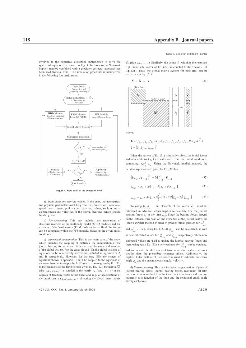
Edgar A. Estupiñan and Ilmar F. Santos
40 / Vol. XXXI, No. 1, January-March 2009 ABCM
involved in the numerical algorithm implemented to solve the system of equations, is shown in Fig. 4. In this case, a Newmark implicit method combined with a predictor-corrector approach has been used (Garcia, 1994). The simulation procedure is summarized in the following four main steps:
Plot Results
Numerical Integration
No
YesYes
No
Yes
Global Matrix System
Input Data- Geometrical and
physical parameters
ti+1 = ti + 2t
t < tfinal
Use a smaller 2tand start again < 1
Updating - Eccentricity,
- Attitude angle, �
Updating- Displacements
- Velocities
FEM ModuleRotor: [M],[K],[D]
MBD Module-Constrain equations- Motion equations
Initial Conditions, t = t0- Displacements
-Velocities
FFF Module-Journal bearing forces
Figure 4. Flow chart of the computer code.
a) Input data and starting values. In this part, the geometrical and physical parameters must be given, i.e., dimensions, rotational speed, mass, inertia, preloads, etc. Starting values, such as initial displacements and velocities of the journal bearings centre, should be also given.
b) Pre-processing. This part includes the generation of structural matrices of the multibody model (MBD module) and the matrices of the flexible rotor (FEM module). Initial fluid film forces can be computed within the FFF module, based on the given initial conditions.
c) Numerical computation. This is the main core of the code, which includes the coupling of matrices, the computation of the journal bearing forces at each time step and the numerical solution of the global system. For the cases (I) and (II), the global systems of equations to be numerically solved are included in appendixes A and B respectively. However, for the case (III), the system of equations shown in appendix C must be coupled to the equations of the rotor. In order to couple the MBD matrix system given by Eq. (21) to the equations of the flexible rotor given by Eq. (22), the matrix M(size ndofndof � ) is coupled to the matrix A (size 1616� ) in the degrees of freedom related to the linear and angular accelerations of the crank centre ( 1q�� , 2q�� , 3q�� , 4q�� ), obtaining the global mass matrix
M~ (size 12�ndof ). Similarly, the vector f , which is the resultant right hand side vector of Eq. (22), is coupled to the vector c of Eq. (21). Thus, the global matrix system for case (III) can be written as in Eq. (31).
cbM ~~~� (31)
where,
� �T�� ������ ,x,,f,f,f,f,N,N,f,f,f BzCzAyAxAzyzByBxBb ;
� �Tndofq,...,q,q �������� 21q
When the system of Eq. (31) is initially solved, the initial forces and accelerations ( 0b~ ) are calculated from the initial conditions, computing:
01
0 tt~~ cM �� . Using the Newmark implicit method, the
iterative equations are given by Eq. (32-34).
� � 11
111 ����� � itititit
~~, cMqb T�� (32)
/ � � 011 1 �� ��� itititit qˆqˆtqq ������ 112 (33)
/ � � 01
2
1 2212 �� ���� ititititit qˆqˆtqtqq ����� ��22 (34)
To compute 1�itq�� , the elements of the vector
1
~�it
c must be
estimated in advance, which implies to calculate first the journal bearing forces bf at the time 1�it . Since the bearing forces depend on the instantaneous position and velocities of the journal centre, the Heun's explicit method is used to predict initial guesses for 0
1�itq�
and 01�it
q . Then, using Eq. (32-34) 11�it
q�� can be calculated, as well
as new estimated values for 11�it
q� and 11�it
q respectively. These new
estimated values are used to update the journal bearing forces and then, using again Eq. (32) a new estimate for 2
1�itq�� can be obtained,
and so on until the difference of two consecutive values becomes smaller than the prescribed tolerance given. Additionally, the explicit Euler method of first order is used to estimate the crank angle
it� and the instantaneous angular velocity.
d) Post-processing. This part includes the generation of plots of journal bearing orbits, journal bearing forces, maximum oil film pressure, minimum fluid film thickness, reaction forces and reaction moments as a function of the time and the rotational crank angle during each cycle.
(16 x 16)
(ndof x ndof)
����
�
����
�
�
����
�
����
�
�
����
�
����
�
�
����
�
����
�
�
�
�
�
�
f
c
q
b
M
A
��
118 Appendix B. Journal papers
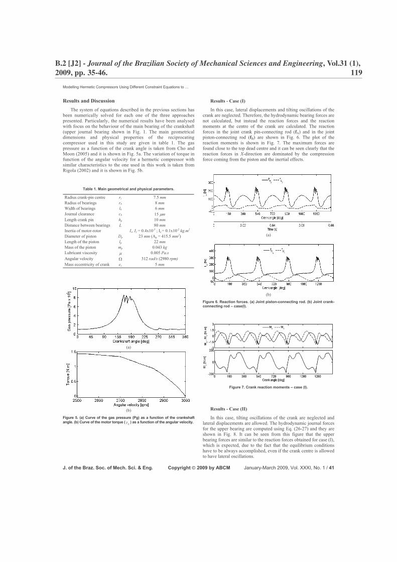
Modelling Hermetic Compressors Using Different Constraint Equations to …
J. of the Braz. Soc. of Mech. Sci. & Eng. Copyright 4 2009 by ABCM January-March 2009, Vol. XXXI, No. 1 / 41
Results and Discussion The system of equations described in the previous sections has
been numerically solved for each one of the three approaches presented. Particularly, the numerical results have been analysed with focus on the behaviour of the main bearing of the crankshaft (upper journal bearing shown in Fig. 1. The main geometrical dimensions and physical properties of the reciprocating compressor used in this study are given in table 1. The gas pressure as a function of the crank angle is taken from Cho and Moon (2005) and it is shown in Fig. 5a. The variation of torque in function of the angular velocity for a hermetic compressor with similar characteristics to the one used in this work is taken from Rigola (2002) and it is shown in Fig. 5b.
Table 1. Main geometrical and physical parameters.
Radius crank-pin centre rc 7.5 mmRadius of bearings rb 8 mmWidth of bearings lb 6 mmJournal clearance cb 15 *mLength crank pin hp 10 mm Distance between bearings L 80 mmInertia of motor-rotor Ix, Iy = 0.4x10⁻³ ; Iz = 0.1x10⁻² kg.m2
Diameter of piston Dp 23 mm (Ap = 415.5 mm2)Length of the piston lp 22 mmMass of the piston mp 0.043 kgLubricant viscosity * 0.005 Pa.sAngular velocity ( 312 rad/s (2980 rpm)Mass eccentricity of crank ec 5 mm
(a)
(b)
Figure 5. (a) Curve of the gas pressure (Pg) as a function of the crankshaft angle. (b) Curve of the motor torque ( z5 ) as a function of the angular velocity.
Results - Case (I)
In this case, lateral displacements and tilting oscillations of the crank are neglected. Therefore, the hydrodynamic bearing forces are not calculated, but instead the reaction forces and the reaction moments at the centre of the crank are calculated. The reaction forces in the joint crank pin-connecting rod (fA) and in the joint piston-connecting rod (fB) are shown in Fig. 6. The plot of the reaction moments is shown in Fig. 7. The maximum forces are found close to the top dead centre and it can be seen clearly that the reaction forces in X-direction are dominated by the compression force coming from the piston and the inertial effects.
(a)
(b)
Figure 6. Reaction forces. (a) Joint piston-connecting rod. (b) Joint crank-connecting rod – case(I).
Figure 7. Crank reaction moments – case (I).
Results - Case (II)
In this case, tilting oscillations of the crank are neglected and lateral displacements are allowed. The hydrodynamic journal forces for the upper bearing are computed using Eq. (26-27) and they are shown in Fig. 8. It can be seen from this figure that the upper bearing forces are similar to the reaction forces obtained for case (I), which is expected, due to the fact that the equilibrium conditions have to be always accomplished, even if the crank centre is allowed to have lateral oscillations.
B.2 [J2] - Journal of the Brazilian Society of Mechanical Sciences and Engineering, Vol.31 (1),2009, pp. 35-46. 119

Edgar A. Estupiñan and Ilmar F. Santos
42 / Vol. XXXI, No. 1, January-March 2009 ABCM
Figure 8. Journal bearing forces – case (II).
The orbit of the journal centre for the upper bearing using the SJB approach is shown in Fig. 9. The orbit obtained has a similar shape compared to predicted orbits of main bearings of internal combustion engines (Ritchie, 1975; Pal, 1988). The maximum fluid film pressure is computed for each crank angle during four cycles, as shown in Fig. 10. It can be observed that the highest values of hydrodynamic pressure in the bearings are found at each cycle around the top dead centre position of the piston, i.e., when the pressure in the cylinder is maximum.
Figure 9. Orbit journal centre – case (II).
Figure 10. Maximum fluid film pressure – case (II).
Results - Case (III)
In this case, lateral displacements and tilting oscillations of the crank are allowed. Therefore, the matrix system of equations of the multibody model is coupled to the equations of the finite elements formulation of the crankshaft. Considering that this study is more focused on the hydrodynamic behaviour of the journal bearings than in the dynamics of the crankshaft, only four finite elements were used for the calculations, which are enough to include the flexible supports (journal bearings), crank and rotor unbalance, and to describe the tilting oscillations of the crank. Moreover, the main interest is to cover frequency range from 0 to 5000 Hz. Using a linearized model for the journal bearings the first and second bending eigenfrequencies of the shaft are around 1050 Hz and 6810 Hz respectively. Following the flow chart of Fig. 4, the global system of equations was solved by using a time step of �t=1e-6s, in order to ensure convergence of the solution.
The fluid film forces computed for the upper and lower bearings are shown in Fig. 11. It can be seen from this figure that the upper bearing forces are similar to the ones obtained for case (II), however, in this case, small transient oscillations occur during the first cycles of the crank rotation. The transient oscillations are more evident in the plot of the lower bearing forces, since the fluid film forces for this bearing are much lower compared to the upper bearing forces. During the numerical simulations, it was noticed that these oscillations are of numerical origin, caused by the initial conditions adopted. The transient response disappears after the first cycles and the system operates under steady-state conditions.
(a)
(b)
Figure 11. Journal bearing forces. (a) Upper bearing, (b) Lower bearing – case (III).
The minimum fluid film thickness for the upper bearing is plotted in Fig. 12a. It is observed in this figure that the lowest values of oil film thickness are found during the gas compression cycle, at approximately 65deg before the piston reaches the top dead centre (i.e., when deg1153� , deg4753� , deg8353� ,…). When the plot of minimum fluid film thickness is compared with the plot of maximum pressure, shown in Fig. 12b, it can be seen that the highest pressures values occur at approximately 30deg after the lowest fluid film thickness is reached during each cycle.
120 Appendix B. Journal papers

Modelling Hermetic Compressors Using Different Constraint Equations to …
J. of the Braz. Soc. of Mech. Sci. & Eng. Copyright 4 2009 by ABCM January-March 2009, Vol. XXXI, No. 1 / 43
(a)
(b)
Figure 12. (a) Minimum fluid film thickness. (b) Maximum pressure – upper journal bearing – case(III).
The effect of including the length of the crank pin (hp) on the behaviour of the upper bearing has been studied through the comparison of orbits and curves of the minimum fluid film thickness, obtained for two different values of hp. Figure 13a shows the journal orbits obtained for cases (II) and (III) using hp = 10mmand hp = 0. It is shown in the figure that the influence of the parameter hp in the orbits is more significant for case (III) than for case (II). This is explained by the fact that in the cases (I) and (II), tilting oscillations of the crank are not allowed, therefore, transversal moments over the crank due to the reaction force fA are equilibrated by the reaction moments MX and MY, as shown in Fig. 7. The influence of the parameter hp on the variation of the minimum fluid film thickness for case (III) can be observed in Fig. 13b. Despite the fact that the difference between the two plots does not seem to be significant, it is found that at some crank positions (e.g., when � = 1180deg) the difference between the two film thicknesses may be as high as 18%. Therefore, in order to estimate more accurately the effect of the tilting oscillations of the crank on the behaviour of the bearings, it is relevant to include the parameter hp in the multibody model of the compressor.
The difference between the maximum hydrodynamic pressures computed by using the SJB and LJB approaches respectively can be significant, as it can be seen in Fig. 14. Thus, in order to ensure a better estimation of the load carrying capacity, and taking into consideration that the bearings of the compressor used for this study are short (lb\rb = 0.75), all the results presented in this section were obtained by using the SJB approach.
(a)
(b)
Figure 13. Effect of the crank pin length (hp). (a) Orbits. (b) Minimum fluid film thickness.
Figure 14. Maximum fluid film pressure using the SJB and LJB approaches.
Conclusions and Further Aspects Three different approaches for the modelling of a hermetic
reciprocating compressor have been analysed in this work. It was found that when the lateral and tilting vibration of the crank are included in the model, more precise estimations of the minimum film thickness are obtained. However, no significant differences were found in the estimation of the hydrodynamic journal bearing forces and the fluid film pressures between the different cases studied. The maximum forces and the minimum film thickness are obtained when the piston is close to the top dead centre. Furthermore, a delay of approximately 30deg between the lowest value of the minimum oil film thickness and the maximum fluid film pressure at each cycle was found. The results showed that the nonlinear behaviour of the orbits increases due to the tilting oscillations of the crank, influenced by the length of the crank pin. The increase of the minimum fluid film thickness and the reduction of the bearing vibrations seem to be feasible by modifying the hydrodynamic lubrication conditions through the implementation of a controllable lubrication system based on the periodic behaviour of the bearing performance. In order to develop such a system, further work will be carried out.
B.2 [J2] - Journal of the Brazilian Society of Mechanical Sciences and Engineering, Vol.31 (1),2009, pp. 35-46. 121

Edgar A. Estupiñan and Ilmar F. Santos
44 / Vol. XXXI, No. 1, January-March 2009 ABCM
Acknowledgments The authors gratefully acknowledge the support given by the
Programme Al�an, the European Union Programme of High Level Scholarships for Latin America, scholarship No. E06D101992CO.
References Cho, J. R. and Moon, S.J., 2005, “A Numerical Analysis of the
Interaction between the Piston Oil Film and the Component Deformation in a Reciprocating Compressor”, Tribology International, Vol.38, pp. 459-468.
Dufour, R., Der Hagopian, J. and Lalanne, M., 1995, “Transient and Steady State Dynamic Behaviour of Single Cylinder Compressors: Prediction and Experiments”, Journal of Sound and Vibration, Vol.181, pp. 23-41.
Frêne, J., Nicolas, D., Degueurce, B., Berthe, D. and Godet, M., 1990, “Lubrification Hydrodynamique”, Ed. Eyrolles, Paris, 488 p.
Garcia de Jalon, J. and Bayo, E., 1994, “Kinematic and Dynamic Simulation of Multibody Systems”, Ed. Springer-Verlag, New-York, 440 p.
Gommed, K. and Etsion, I., 1993, “Dynamic Analysis of Gas Lubricated Reciprocating Ringless Pistons - Basic Modelling”, Journal of Tribology,Vol.115, pp. 207-213.
Hamrock, B. J., 1991, “Fundamental of Fluid Film Lubrication”, NASA Reference Publication, USA, 635 p.
Kim, T. J. and Han, J. S., 2004, “Comparison of the Dynamic Behavior and Lubrication Characteristics of a Reciprocating Compressor Crankshaft in Both Finite and Short Bearing Models”, Tribology Transactions, Vol.47, No.1, pp. 61-69.
Longo, G. and Gasparella, A. 2003, “Unsteady State Analysis of the Compression Cycle of a Hermetic Reciprocating Compressor”, International Journal of Refrigeration, Vol.26, pp. 681-689.
Nelson, H. D. and McVaugh, J. M., 1976, “The dynamics of Rotor-Bearing Systems Using Finite Elements”, Journal of Engineering for Industry, Vol.98, pp. 593-600.
Pal, R., Sinhasan, R. and Singh, D.V, 1988, “Analysis of a Big-End Bearing - a Finite Element Approach”, Wear, Vol.121, No.1, pp. 117-120.
Rasmussen, B.D., 1997, “Variable Speed Hermetic Reciprocating Compressors for Domestic Refrigerators”, Ph.D. Thesis, Technical University of Denmark, Lyngby, Denmark, Vol.1, 158 p.
Rigola, S. J., 2002, “Numerical Simulation and Experimental Validation of Hermetic Reciprocating Compressors”, Ph.D. Thesis, Universidad Politécnica de Cataluña, Barcelona, Spain, 109 p.
Ritchie, G.S., 1975, “The Prediction of Journal Loci in Dynamically Loaded Internal Combustion Engine Bearings”, Wear, Vol.35, No.2, pp. 291-297.
Santos, I. F., 2001, “Dinâmica de Sistemas Mecanicos”, Ed. Makron Books, Sao Paulo, Brasil, 272 p.
Appendix A.
Full Matrix of the Multibody Dynamic Model – Case (I): / 0 � � � �IcIbI A �
�����������
�
�����������
�
�
�����������
�
�����������
�
�
����
�
�
�
�����������
�
�����������
�
�
�����������
�
�����������
�
�
�
�
�
�
�
��
��
�����
��
��������
5
����
�
�
����
������
���
��
slsrclcr
gmrgm
gmsrm
crmgm
AP
x
MMffffffNNfff
lccrlssr
Icrsrcsrsc
Isrmlclsl
crmsrmm
m
C
C
z
crcr
c
cr
crcr
crcr
p
pg
B
C
C
C
C
C
A
A
A
Z
Y
B
B
B
C
C
cCC
C
crcrcr
crcr
crcrcr
p
Y
X
Z
Y
X
Z
Y
X
Z
Y
X
Z
Z
22
22
2
2
000
00
0
0000000000000010000000000000
0000000000000000000000000000000000000000
00000000000000000000000000000010010000000000001001000000
00000001001000000000000010000100
00000000100001000000000100001
00000000000101000000000000001010000000000000001
��
��
�
�
��
��
��
122 Appendix B. Journal papers
Modelling Hermetic Compressors Using Different Constraint Equations to …
J. of the Braz. Soc. of Mech. Sci. & Eng. Copyright 4 2009 by ABCM January-March 2009, Vol. XXXI, No. 1 / 45
Appendix B
Full Matrix of the Multibody Dynamic Model – Case (II): / 0 � � � �IIcIIbII A �
�����������
�
�����������
�
�
�����������
�
�����������
�
�
����
�
�
�
�����������
�
�����������
�
�
�����������
�
�����������
�
�
�
�
�
�
��
����
���
�����
��
Y
X
C
C
z
crcr
c
cr
crcr
crcr
p
pg
C
C
B
C
C
C
A
A
A
Z
Y
B
B
B
C
C
c
c
cCC
C
crcrcr
crcr
crcrcr
p
FF
slsrclcr
gmrgmgm
srmcrm
gm
AP
yx
x
MMffffNNfff
mm
lccrlssr
Icrsrcsrsc
Isrmlclsl
crmsrmm
m
Y
X
Z
Z
Y
X
Z
Y
X
Z
Z
��������
5
����
�
�
����
������
���
��
22
22
2
2
000
0
00000000100000000000000010000010000000000000
011000000000000000000000000000000000000000000000000000000000000000000000000000000000000011000000000000000100001000000000010000100000000010000100000000000101000000000000001010000000000000001
��
��
�
�
��
��
��
��
��
Appendix C
Full Matrix of the Multibody Dynamic Model – Case (III): / 0 � � � �IIIcIIIbIII A �
�����������
�
�����������
�
�
�����������
�
�����������
�
�
���
��
�
�
�����������
�
�����������
�
�
�����������
�
�����������
�
�
�
�
�
�
�
������
��
���
���������
��
��
���
16
15
14
13
2
2
12111098
13
12
11
765
4
321
00
0
0
00000000000000000000
000000001000000000000000100000
1000000000000011000000000
000000000000000011000000000000000000000000000000000000000000100001000000000010000100000000010000100000000000101000000000000001010000000000000001
CC
CCcIgm
gmrgm
srmcrm
gm
AP
yx
x
ffffNNfff
cIscICCCCCsIccIrChrChrCh
mm
CClcCClsscr
sIcsemsemIICCC
Isrmlclsl
crmsrmm
m
zc
c
crcr
cr
crcr
crcr
p
pg
C
C
B
C
A
A
A
Z
Y
B
B
B
cc
cccpcpcp
c
c
c
cccccmc
crcrcr
crcr
crcrcr
p
Z
Z
Z
Y
X
Z
Y
X
YY
XX
ZZZ
Z
5�
����
�
�
�
����
���
�
���
��
��
�
�
��
��
��
��
��
��
��
B.2 [J2] - Journal of the Brazilian Society of Mechanical Sciences and Engineering, Vol.31 (1),2009, pp. 35-46. 123

Edgar A. Estupiñan and Ilmar F. Santos
46 / Vol. XXXI, No. 1, January-March 2009 ABCM
where:
)(
)()(
)()(
9
8
7
6
5
4
3
2
1
������
��������
�����
�������
�
sccsshcsrCcchsrC
sshccsrCcchcscssrC
ccsssrCchcsrC
cssscrCsssccrC
scrC
pc
pc
pc
pc
c
pc
c
c
c
��������
��������
�����
�����
��
))()(()())()(()(
2)(2)(2)()()(
)2()()(
)(
016
15
222214
2213
12
11
10
XZY
ZYX
ccc
ccc
cpcc
pcpccc
ccp
ccr
ccr
pc
IIccsssssccICIIsccscsccsICscsrschcccrssccsr
cshcssrcshcssrscrcssscrslCclccssrccrshC
sssccemCscemC
cscsshccrC
�������������������������������������
�����������������������
����
����
������������������������
�����������������������������
�����������
������
����������
����������
������
����
�����
-------------------------------------------------------
124 Appendix B. Journal papers

B.3 [J3] - Tribology International, Vol. 42 (10), 2009, pp. 1478-86. 125
B.3 [J3] - Tribology International, Vol. 42 (10), 2009, pp. 1478-86.

Linking rigid multibody systems via controllable thin fluid films
E.A. Estupinan, I.F. Santos �
Technical University of Denmark, Department of Mechanical Engineering, Nils Koppels Alle, 404, Kgs. Lyngby DK-2800, Denmark
a r t i c l e i n f o
Article history:
Received 8 July 2008
Received in revised form
22 January 2009
Accepted 7 May 2009Available online 15 May 2009
Keywords:
Controllable thin fluid film
Hybrid lubrication
Fluid film journal bearing
Reciprocating compressor
a b s t r a c t
This work deals with the mathematical modelling of multibody systems interconnected via thin fluid
films. The dynamics of the fluid films can be actively controlled by means of different types of actuators,
allowing significant vibration reduction of the system components. In this framework, this paper gives a
theoretical contribution to the combined fields of fluid–structure interaction and vibration control. The
methodology is applied to a reciprocating linear compressor, where the dynamics of the mechanical
components are described with help of multibody dynamics. The crank is linked to the rotor via a thin
fluid film, where the hydrodynamic pressure is described by the Reynolds equation, which is modified
to accommodate the controllable lubrication conditions. The fluid film forces are coupled to the set of
nonlinear equations that describes the dynamics of the reciprocating linear compressor. The system of
equations is numerically solved for the case when the system operates with conventional hydrodynamic
lubrication and for several cases of the bearing operating under controlled hybrid lubrication
conditions. The analysis of the results is carried out with focus on the behaviour of the journal orbits,
maximum fluid film pressure and minimum fluid film thickness.
& 2009 Elsevier Ltd. All rights reserved.
1. Introduction
The feasibility of applying active lubrication to the mainbearings of a hermetic reciprocating compressor is studied in thiswork, with the help of multibody dynamics and fluid film theory.Small-scale reciprocating compressors are of common use tocompress coolant gas in household refrigerators and air condi-tioners. This type of compressors have pistons that are drivendirectly through a slider-crank mechanism, converting the rotat-ing movement of the rotor to an oscillating motion, as illustratedin Fig. 1. The performance of the bearings affects key functions ofthe compressor, such as durability, noise, and vibrations.Therefore the study and optimization of the dynamic behaviourof reciprocating compressors, taking into account thehydrodynamics of bearings, can be of significant importance forthe development of new prototypes. Several studies related to themodelling of small reciprocating compressors can be found in theliterature [3,4], however, only a few of them have incorporated intheir models the dynamics of the fluid films. For instance, a studythat includes the coupling of fluid–structure dynamics to analysethe dynamics of the piston is described in Ref. [5]. In the work ofRef. [6], a model of the coupled dynamic behaviour of the pistonand crankshaft is developed and some comparisons between afinite-width bearing model and a short-width bearing approachare included in the study. In contrast to previous studies, in thiswork a multibody dynamic model that represents the dynamics of
the main mechanical components of a reciprocating compressor iscoupled to the dynamics of the fluid film bearings, and theanalysis is focused on the performance of the upper bearingworking under hydrodynamic and hybrid (controllable)lubrication conditions. In a reciprocating machine, the lubricantfilms surrounding the main bearings commonly have to supportinertial loads, crankshaft unbalance forces and the reciprocatingforces coming from the gas pressure dynamics. The behaviour ofthese forces is quasi-periodic, since some changes in magnitudeand frequency can occur from one cycle to the next, depending onthe operating conditions. It causes that the centre of the journalbearing does not conserve a steady position, generatingunwanted vibrations of the journal. The most common approachused for the analysis of dynamically loaded bearings is themobility technique, which was developed more than 40 years ago[1]. Other methods involving bearing flexibility and thermaleffects have been developed in the last two decades [2], howeverthey are characterized by a higher computational complexity. Inthis study, the fluid film theory based on hydrodynamiclubrication conditions has been used to describe the governingequation of the fluid pressure distribution along the bearingsurface, since the analysis is more focused on studying thefeasibility of actively modifying the hydrodynamic fluid filmsthrough radial oil injection (controllable hybrid lubrication), thanin the estimation of the elastic deformations of the system. Onerefers to hybrid lubrication when the hydrostatic and thehydrodynamic lubrication are simultaneously combined in ajournal bearing. When part of the hydrostatic pressure isdynamically modified, one refers to active lubrication [7].Besides the operational conditions, the performance of a hybrid
ARTICLE IN PRESS
Contents lists available at ScienceDirect
journal homepage: www.elsevier.com/locate/triboint
Tribology International
0301-679X/$ - see front matter & 2009 Elsevier Ltd. All rights reserved.
doi:10.1016/j.triboint.2009.05.009
� Corresponding author. Tel.: +4545256269; fax: +4545931475.
E-mail address: [email protected] (I.F. Santos).
Tribology International 42 (2009) 1478–1486
126 Appendix B. Journal papers

journal bearing depends on several geometric parameters,such as position and diameter of the orifices, bearing aspectratio and axial land width ratio [8,9]. Several studies havebeen carried out to geometrically optimize the design of hybridjournal bearings for specific configurations and for differentexternal load conditions [10,11]. Depending on the load andspeed working conditions, several types of configurations arepossible for hybrid journal bearings. Particularly, it has beenshown by Rowe [9], that for hybrid performance and easymanufacture, hole-entry type bearings with holes disposedcircumferentially along two rows may offer advantages overother configurations.
The present work compares the tribological performance of theupper journal bearing of a compressor working with conventional
ARTICLE IN PRESS
Fig. 2. Geometry and reference systems. Left: illustration of the main constraint equation; right: reference frames and rotation angles.
Nomenclature
ab axial land (m)�ab axial land width ratio, �ab ¼ ab=lbAp transversal area of the piston (m2)cb clearance of bearing (m)do diameter of orifices (m)ec mass eccentricity of the crank (m)FB finite-width journal bearingf vector of reaction forces (N)fb vector of journal bearing forces (N)hðj; tÞ oil film thickness (m)l length (m)lb width of bearing (m)LJB long-width journal bearingmc mass of the crank (kg)mcr mass of the connecting rod (kg)mp mass of the piston (kg)Pg gas pressure inside the cylinder (Pa)pðj; z; tÞ fluid film pressure distribution (Pa)Pinj injection pressure (Pa)r radius (m)SJB short-width journal bearingTi transformation matrix in the angle i
U tangential velocity (m/s)a rotation angle of the connecting rod (rad)� eccentricity ratiol bearing aspect ratio, l ¼ lb=2rbm oil film viscosity (Pa s)f attitude angle (rad)O angular velocity of the rotor (rad/s)r fluid density ðkg=m3Þtz motor shaft torque (Nm)y rotational angle of the crank (rad)Y angle measured from X axis (rad)
Subscripts
A;B;C relative to the points A, B or C, respectivelyBi relative to the i-th moving reference frameb relative to the bearingsc relative to the crankcr relative to the connecting rodI relative to the inertial reference framej relative to the journalo relative to the orifices
Fig. 1. Schematic draw and general view of a hermetic reciprocating compressor.
E.A. Estupinan, I.F. Santos / Tribology International 42 (2009) 1478–1486 1479
B.3 [J3] - Tribology International, Vol. 42 (10), 2009, pp. 1478-86. 127

hydrodynamic lubrication and with four different configurationsof hybrid lubrication, proposing some rules for the variation of theinjection pressure in function of the crank angle. The equations ofmotion for the reciprocating mechanism are developed usingmultibody dynamics. The crank and rotor are interconnectedvia a thin fluid filmwhere the hydrodynamic pressure distributionis described by the Reynolds equation, which is modified inorder to include the dynamics of the active lubrication andnumerically solved by means of the finite-difference method. Theanalysis of the results is focused on the behaviour of the journalorbits, maximum fluid film pressure and minimum fluid filmthickness.
2. Mathematical modelling
In this section the formulation of representative equationsdescribing the mathematical model for a hermetic compressor isdeveloped. The motion equations for the piston-connectingrod–crank system are formulated with the help of multibodydynamics theory, using Newton–Euler’s method and using a framenotation of common use in multibody dynamics [12–14]. Fig. 2shows a sketch indicating the reference frames and the mainangles of rotation (b, G, y and a). In order to be able to describe allthe representative vectors, one inertial reference frame ðIXYZÞ andfour moving reference frames ðBiÞ have been defined. The inertialreference frame is attached to the centre of the bearing (point O),the moving reference frames B1ðX1Y1Z1Þ, B2ðX2Y2Z2Þ andB3ðX3Y3Z3Þ are attached to the crank and the moving referenceframe B4ðX4Y4Z4Þ is attached to the connecting rod. With the helpof the geometrical transformation matrices Tb, TG, Ty and Ta anyvector can be easily transformed from one reference frame toanother. According to Fig. 2, the main constraint equation of thesystem is given by
IxpþIl¼IrþIc (1)
where Ixp ¼ fxB;0;�hpgT ; Il ¼ f�lcr cosa; lcr sina;0gT ; Ir ¼ TTb � TT
C�TTy � B3r; B3
r ¼ frc ;0;�hpgT ; and Ic ¼ fxc ; yc ;0gT .The equations of motion for each body are given by
Eqs. (2)–(6). The force equations are described in the inertialreference frame and the moment equations of the crank and theconnecting rod are described in the moving reference frames B3
and B4, respectively.
� Force equation—crank:XIf ¼ mc � I �ac ) IfA þ Ifub þ Ifb ¼ mcf€xc ; €yc;0gT (2)
where Ifub is the vector of the crank unbalance force and Ifb isthe vector of the dynamic journal bearing forces.
� Moment equation—crank:
XB3MC ¼ B3
r � B3fA þ B�3s ¼ B3
Icd
dtðB3xÞ
þ B3x � ðB3
IC � B3xÞ þmc�B3 �rC�cm�B3aC (3)
where B3fA ¼ Ty � TC � Tb�IfA; B3
s ¼ f0;0; tzgT ; and
B3�rC�cm ¼ fec ;0;0gT .
� Force equation—connecting rod:XIf ¼ mcr � I �acr ¼ IfA þ IfB (4)
where
I�acr ¼ IaBþI _a�I _a�I �rcrþI €a�I �rcr
¼€xB þ �rcrð _a2 cosaþ €a sinaÞ
�rcrð €a cosa� _a2 sinaÞ0
8>><>>:
9>>=>>;.
� Moment equation—connecting rod
XB4MB ¼ B4
I � B4fA ¼ B4
Icrd
dtðB4
_aÞþB4
_a� ðB4 IcrB4 _aÞ þmcr � B4 �rcr � B4aB (5)
where B4fA ¼ Ta�IfA; B4aB ¼ Ta�IaB; IaB ¼ f€xB;0;0gT .
� Force equation—pistonXIfB ¼ mp�IaB¼IfBþIfNþIfp (6)
where Ifp ¼ fPgAp;0;0gT .
The equations of motion may be written in a matrix form as in(7), where the vector �b includes the unknown reaction forces,reaction moments and accelerations of the system:
�A � �b ¼ �c (7)
where
�b ¼ ff Bx ; f By ; f Bz;Ny;Nz; f Ax
; f Ay; f Az
; f Cz; €y; €xB; €a; €xc; €ycgT
3. Fluid film forces
The equations that govern the dynamics of the fluid films in adynamically loaded journal bearing, for the conventional hydro-dynamic lubrication case and for the active lubrication case, arepresented. The main geometrical relations of a fluid film journalbearing are shown in Fig. 3. The governing equation for thepressure distribution of the oil film in journal bearings can beobtained from the standard reduced form of the Reynoldsequation for elastohydrodynamic lubrication [15], given by
@
@x
rh3
12m@p
@x
!þ @
@z
rh3
12m@p
@z
!¼ @
@x
rhðUj � UbÞ2
� �þ @ðrhÞ
@t(8)
Eq. (8) describes the flow in the journal bearing in the domain0 � x � 2prb and �lb=2 � z � lb=2. For the upper bearing ofthe compressor: Uj ¼ Orb and Ub ¼ 0. The fluid film thicknessmeasured from j ¼ 0 can be calculated using: h ¼ cbð1þ � cosjÞ,where j is the angle measured from the location of the maximumfluid film thickness, as shown in Fig. 3. Thus, using the coordinatetransformation x ¼ rbj in Eq. (8) and assuming that the fluid isisoviscous, Newtonian and incompressible, the Reynolds equationcan be rewritten as
@
@jh3
m@p
@j
!þ r2b
@
@z
h3
m@p
@z
!¼ 12cbr
2b
_� cosjþ � sinj _f�O2
� �� �
(9)
In dynamically loaded bearings the eccentricity and attitudeangle varies through the loading cycle. Therefore, as seen inEq. (9), the pressure distribution may be only determined if thenormal squeeze velocity (_�) and the rotational velocities ( _f and O)
ARTICLE IN PRESS
Fig. 3. Journal bearing geometry. Left: front view; right: side view—unwrapped
bearing.
E.A. Estupinan, I.F. Santos / Tribology International 42 (2009) 1478–14861480
128 Appendix B. Journal papers

are known at any time during each cycle. The journal bearingforces can be calculated by integrating the pressure distributionover the bearing surface as
Fx
FZ
( )¼Z 2p
0
Z lb=2
�lb=2p
cosjsinj
( )rb dz dj (10)
When the computation of the fluid film forces is limited to theconvergent film the solution is known as the half Sommerfeldsolution. Another well known cavitation condition is the Gumbelcondition in which the Reynolds equation is first solved subjectedto the specified pressures at the bearing boundaries and then ifsubambient pressures appear they are neglected. Although the useof the Gumbel cavitation condition does not satisfy the continuityof flow at film rupture as well as reformation, it provides acceptableaccuracy in the estimation of oil film pressure and bearing loadcapacity with low computational cost [17]. However, in caseswhere an acceptable estimation of oil flow is required, a moreaccurate cavitation condition should be used, such as theJakobsson–Floberg and Olsson cavitation condition [18], whichconserves mass both at the rupture and the reformation boundariesbut substantially increases the computational cost.
Analytical solutions of Eq. (9) may be obtained only for limitedcases: a short-width journal bearing ðSJBÞ and an infinitive long-width journal bearing ðLJBÞ. The short journal bearing approachassumes that the variation of pressure is more significant in theaxial direction than in the circumferential direction and thereforethe first term on the left side of Eq. (9) can be neglected. For aninfinitely long-journal-bearing solution the pressure in the axialdirection is assumed to be constant, therefore, the side-leakageterm, i.e., the second term on the left side in (9), can be neglected.Thus, using the Gumbel cavitation condition, the analyticalexpressions to calculate journal forces in x, Z coordinates usinga short-journal-bearing approach and an infinitely long journalapproach are given by the equations listed in Table 1.
3.1. The modified Reynolds equation for active lubrication
The governing equation for the hydrodynamic pressuredistribution of an active lubricated journal bearing can beobtained from the Navier Stokes equation and the continuityequation by accommodating in the assumed boundary conditionsthe velocity profile of the oil injection, which is described in detailin Refs. [19,20]. Thus, the pressure distribution for a journalbearing with radial oil injection through orifices located at ðji; ziÞalong the bearing surface is governed by
@
@jh3
r2bm@p
@j
!þ @
@z
h3
m@p
@z
!� 3
mlo
Xsi¼1
iðj; zÞ � p
¼ 12cb _� cosjþ � sinj _f�O2
� �� �� 3
mlo
Xsi¼1
iðj; zÞ � PinjðtÞ
(11)
where
iðj; zÞ ¼d2o4
� R2 if R2 � d2o=4
0 if R2 � d2o=4
8><>:
and R2 ¼ r2bðj�jiÞ2 þ ðz� ziÞ2.In this equation, the function iðj; zÞ is used to describe
mathematically the problem and is physically related to theposition of the orifices. In other words, this function will bedifferent than zero inside the orifices region and will be zeroelsewhere. On the other hand, PinjðtÞ gives the injection pressure ateach orifice in function of time. It can be observed that when thebearing is operating only under conventional hydrodynamiclubrication, the function iðj; zÞ ¼ 0 and Eq. (11) changes intothe traditional Reynolds equation given by (9).
From the point of view of active lubrication and specificallyconsidering the case of a dynamically loaded journal bearing, Pinj
must be dynamically controlled. However, and taking into accountthe periodic behaviour of the load acting on the upper bearing,this work is more focused on the evaluation of the tribologicalperformance of the bearing operating with different configura-tions of radial oil injection, than in the design of the controlsystem. Thus, the modified Reynolds equation (11) is solved ateach time step assuming that the oil injection pressures for eachone of the orifices are known and are given in function of theinstantaneous crank angle. In order to control the bearing oilinjection pressures, different alternatives may be considered, suchas mechanical cam systems, hydraulic servovalves [7,19] andpiezoelectric nozzles [21,22].
4. Numerical procedure
The steps to obtain the fluid film forces, reaction forces androtor equilibrium position in function of time, are summarized inthe following main steps:
� Pre-processing: Based on the geometric and physical para-meters of the system (i.e., dimensions, rotational speed,inertias, etc.) and on the kinematic initial conditions, theinitial system of equations for the multibody dynamic modelcan be defined.
� Solution of the Reynolds equation: The Reynolds equation forconventional hydrodynamic lubrication (9) can be solvedanalytically (for the SJB and LJB approaches) by using theexpressions of Table 1. However, when a solution for a finite-width bearing (FB) is required or when the Reynolds equationincludes the terms that account for the active lubrication, as inEq. (11), numerical methods have to be used. In this work, themodified Reynolds equation is discretized via finite differencesand solved for each time step by using a direct system equationsolver based on the well known LU factorization method [23].To compute the fluid film forces, the pressure distribution isnumerically integrated over the journal surface, as in Eq. (10),using the Simpson Method. To represent the fluid film forces inthe inertial reference frame, a standard transformation in theangle f is used, i.e., Ifb ¼ TffFx; FZgT. In order to discretize themodified Reynolds equation for active lubrication, a non-uniform grid is used to be able to refine the mesh over the areawhere the orifices for oil injection are located and to obtainmore accurate results for the film pressures and the minimumfluid film thicknesses. If the bearing surface is discretized in jand z directions with a non-uniform grid of m� n nodes,respectively, and assuming that the bearing is well aligned (i.e.,@h=@z ¼ 0) and the viscosity of the fluid film keeps constant,
ARTICLE IN PRESS
Table 1Analytical equations to calculate journal bearing forces, Ref. [16].
Short-width journal bearing (SJB)
Fx ¼ �rbml3b
2c2b ð1� �2Þ2p_�ð1þ 2�2Þffiffi½p �ð1� �2Þ þ 2�2ðO� 2 _fÞ� �
FZ ¼ rbml3b�
2c2b ð1� �2Þ24_�þ p
2ðO� 2 _fÞ ffiffi½p �1� �2
h i
Long-width journal bearing (LJB)
Fx ¼ �12mr3b lbc2b
�2ðO� 2 _fÞð2þ �2Þð1� �2Þ þ
_�ð1� �2Þ3=2
p2� 8
pð2þ �2Þ
� �" #
FZ ¼ 12mr3b lbc2b
p�ðO� 2 _fÞ2ð2þ �2Þ ffiffi½p �1� �2
þ 2�_�ð2þ �2Þð1� �2Þ
" #
E.A. Estupinan, I.F. Santos / Tribology International 42 (2009) 1478–1486 1481
B.3 [J3] - Tribology International, Vol. 42 (10), 2009, pp. 1478-86. 129

the Reynolds equation in finite differences is given by
Dm;npm�1;n þLm;npmþ1;n þ}m;npm;n þrm;npm;n�1 þ Dm;npm;nþ1
¼ 12cbr2b
_� cosjm;n þ � sinjm;n_f�O
2
� �� �
� 3r2bmlo
Xsi¼1
im;n
�Pinj (12)
where
Dm;n ¼ 1
Djm þ Djm�1
�3h2m;n
m@h
@j
����m;n
þ 2h3m;n
mDjm
" #
Lm;n ¼ 1
Djm þDjm�1
3h2m;n
m@h
@j
����m;n
þ 2h3m;n
mDjm
" #
}m;n ¼ � 2h3m;n
m1
Djm þ Djm�1
1
Djm
þ 1
Djm�1
� ��
þ r2bDzn þ Dzn�1
1
Dznþ 1
Dzn�1
� �#� 3r2bmlo
Xsi¼1
im;n� pm;n
rm;n ¼ 2h3m;nr2b
mDzn�1
1
Dzn þ Dzn�1; Dm;n ¼ 2h3m;nr
2b
mDzn1
Dzn þDzn�1
In order to solve Eq. (12), suitable boundary conditions must bedefined. Since the boundary pressure at the bearing edges isatmospheric, it may be taken as zero: p ¼ 0; for z ¼ 0 and lb.Along the j direction, the Reynolds equation is solvedconsidering that p ¼ 0 at j ¼ 0 and 2p, and if subambientpressures appear they are replaced by zero, assuming theGumbel boundary conditions.
� Numerical solution of the global system: In order to solve theglobal system given by Eq. (7) and to obtain the reaction forcesand accelerations of the system, the fluid film forces must becalculated and updated at each time step in the vector �c.However, the calculation of the fluid film forces at the time tiþ1
depends on the velocity and position of the crank centre at tiþ1,which must be estimated previously. Therefore, in this work ascheme based on the implicit Newmark method combinedwith a predictor–corrector approach has been used [24]. Thus,for each time step initial estimations of the position andvelocity of the crank centre are obtained by using the Heun’sexplicit method, which allows to compute the fluid film forcesbased on the initial guess values and to solve the global systemat the time tiþ1. Then, by using the implicit Newmark methodnew estimations of the velocity and displacement of the crankcentre can be calculated and used to update the journalbearing forces in the global system, which is solved again, andafter a few iterations the difference between two consecutivevalues becomes smaller than the prescribed tolerance and thecomputation of the global system is moved forward to newtime step.
� Post-processing: After the global system is solved for severalcycles of the compressor, plots of all the variables can begenerated in function of the time or the crank angle. For thepurpose of this work, the main plots of interest are the plots ofthe journal orbits, the minimum fluid film thickness, themaximum film pressure and the film pressure distribution.
5. Numerical results
The main geometrical dimensions and physical properties ofthe reciprocating compressor used for the numerical simulationsare given in Table 2. The curves of variation of the gas pressureinside the cylinder and the motor torque are shown in Figs. 4
and 5, respectively. The numerical results presented in this sectionare obtained from the solution of the global system of equationsand the analysis is centred on the upper journal bearing of thecompressor.
5.1. Comparison between analytical and numerical solutions of the
Reynolds equation
The results obtained for the upper journal bearing, operatingunder conventional hydrodynamic lubrication and by usinganalytical and numerical solutions of the Reynolds equation arepresented in this section. The journal bearing forces areanalytically computed by using the equations of Table 1, andnumerically calculated by using finite differences. The orbitsobtained using the analytical SJB approach and using thenumerical solution for a finite-width bearing are shown inFig. 6. It can be observed that the shape of the orbits is similarin both cases, however, higher eccentricities are found by usingthe finite-width bearing approach, which can be explained by theassumption of neglecting the variation of pressure in thecircumferential direction with the SJB approach. A plot thatcompares the maximum fluid film pressures by using analyticaland numerical solutions of the Reynolds equation is presented inFig. 7. It can be observed that the maximum film pressuresobtained with the LJB approach are much lower than the pressuresobtained with the other approaches. Since these results are for a
ARTICLE IN PRESS
Table 2Main geometrical and physical parameters of the compressor.
Radius crank-pin centre (rc) 7.5 (mm)
Mass of crank (mc) 0.1 (kg)
Inertia of crank (Icz ) 5� 10�3 (kgm2)
Mass of connecting rod (mcr) 0.1 (kg)
Inertia of connecting rod (Icrz ) 1:7� 10�5 (kgm2)
Diameter of piston (Dp) 23 (mm)
Mass of piston (mp) 0.043 (kg)
Bearing aspect ratio (l) 0:375;0:75;1
Land width ratio (�ab) 0:1; 0:15;0:2
Journal clearance (cb) 15m (m)
Fluid viscosity (m) 0.005 (Pa s)
Angular velocity (O) 312 (rad/s)
Diameter (do)/length orifices (lo) 1.5; 20 (mm)
Pg
[Pa
× 1
05 ]
0 45 90 135 225 270 3150
2
4
6
8
10
�c [deg]
180 360
Fig. 4. Cylinder gas pressure [5].
τ z [
N.m
]
2500 2600 2800 29000
0.5
1
1.5
Ω [rpm]
30002700
Fig. 5. Motor torque characteristic curve [4].
E.A. Estupinan, I.F. Santos / Tribology International 42 (2009) 1478–14861482
130 Appendix B. Journal papers

bearing of short dimensions ðl � 0:5Þ, the more realisticestimations of the maximum film pressure are obtained withthe analytical SJB approach and the numerical solutions for afinite-width bearing. To make sure of the correctness of thenumerical solutions obtained, a convergence analysis was carriedout. It was found that using a grid with nj ¼ 90 and nz ¼ 21 nodesfor the solution of the Reynolds equation, and using a time step ofDt ¼ 2� 10�6 s for the solution of the global system, goodapproximations for the minimum fluid film thickness and thepressure distribution can be obtained.
5.2. Influence of the bearing geometric parameters, l and �ab
In this section, the influence of the bearing aspect ratio and theaxial land ratio on the bearing performance is analysed for
conventional hydrodynamic lubrication and hybrid lubrication con-ditions. Fig. 8 illustrates the influence of the parameter l on the orbitof the bearing, the minimum fluid film thickness and the maximumfluid film pressure. It can be observed that with a larger aspect ratiothe minimum fluid film thickness becomes larger and the maximumpressure lower, which means that the journal orbit is generated closerto the centre of the bearing, which is expected due to the increase ofthe bearing area supporting the external load. The fluid film pressuredistributions at four different crank angles during one cycle, for abearing of l ¼ 0:75, are shown in Fig. 9. It can be observed from thisfigure that the maximum oil film pressures are located at the middleof the bearing along the width direction, and in the range of180 � Y � 225, along the circumferential direction. For the casewhen lubricant is injected through orifices located atYo ¼ 180 with�ab ¼ 0:2 and Pinj ¼ 2MPa, the effect of the parameter l on the fluidfilm thickness is shown in Fig. 10. If Figs. 10 and 8(b) are compared, itcan be observed that for the cases with l ¼ 0:5 and 0:375, theinfluence of the injection pressure on the minimum fluid filmthickness is minimum, due to the fact that the fluid film pressuregenerated hydrodynamically is higher than the oil injection pressure.When the bearing aspect ratio is higher ðl ¼ 0:75Þ, the hydrodynamicfilm pressure becomes lower, and therefore, the influence of the radialoil injection Pinj ¼ 2MPa becomes more significant, as seen in Fig. 10.The influence of the axial land width ratio ð �abÞ on the minimum fluidfilm thickness for the same hybrid lubrication conditions is shown inFig. 11. It can be seen that the minimum fluid film thickness is notsignificantly affected by the change of �ab, specially during the timeswhere the lowest film thicknesses are found. Some studies related tothe geometrical optimization of hybrid journal bearings have shownthat typical values for the bearing aspect ratio of hybrid bearings are:0:75 � l � 1, and for the axial land width ratio: 0:1 � �ab � 0:4 [9,11].It has been shown in Ref. [11] that a hybrid bearing with l ¼ 1 and�ab ¼ 0:2 is a good configuration for a bearing with high load carryingcapacity.
5.3. Hybrid journal bearing
The results obtained for the compressor upper bearingoperating with hybrid lubrication conditions are included in thissection. In order to define appropriate angular position of orificesand injection pressures for the upper bearing working with hybridlubrication conditions, the results obtained previously for theconventional hydrodynamic bearing can be used. For instance, itcan be seen from the plots of orbits and pressure distributions,
ARTICLE IN PRESS
Y[�m] Y[ �m]
X [�m
]
-15-10-50 -15-10-50
-15
-10
-5
0
-15
-10
-5
0
Fig. 6. Journal bearing orbits—conventional hydrodynamic lubrication. (a)
Analytical solution—SJB approach; (b) numerical solution—FB, l ¼ 0:375.
Fig. 7. Maximum film pressure using analytical and numerical solutions—conven-
tional hydrodynamic lubrication ðl ¼ 0:375Þ.
X [�m
]
h min
[�m
]p
[MPa
]
λ = 0.375
λ = 0.5
λ = 0.75
λ = 1
0 360 540 720
0 180 360 540
-15-10-50 0
5
10
15
0
5
10
15-15
-10
-5
0
Y [�m]
�c [deg]
720
180
Fig. 8. Influence of the bearing aspect ratio l—conventional hydrodynamic lubrication; (a) journal orbits; (b) minimum film thickness; (c) maximum film pressure.
E.A. Estupinan, I.F. Santos / Tribology International 42 (2009) 1478–1486 1483
B.3 [J3] - Tribology International, Vol. 42 (10), 2009, pp. 1478-86. 131

shown in Figs. 8 and 9 that modifying the hydrodynamiclubrication by injecting oil through orifices located along thethird quadrant of the bearing (i.e., 180 � Y � 270), the maximumhydrodynamic pressure may be reduced and the minimum filmthickness increased. The effects of changing the angular locationof the injection holes and the oil injection pressures on theminimum film thickness, when others geometrical and physicalparameters are kept constant, are analysed in order to findoptimal hybrid lubrication configurations. Fig. 12 shows theminimum fluid film thickness computed for different angularpositions of the orifices, assuming a constant injection pressureduring the entire cycle. It can be seen from the cases analysedthat, when the orifices are located at Yo ¼ 180 and 210 and oilis injected at Pinj ¼ 2MPa, the lowest fluid film thickness may beincreased up to 56% and 25%, respectively, compared to
conventional hydrodynamic lubrication. On the other hand, theeffect of using different oil injection pressures (with a constantvalue through each operating cycle of the compressor) on the
ARTICLE IN PRESS
p [M
Pa]
p [M
Pa]
p [M
Pa]
p [M
Pa]
Z [mm]
�c = 0° (� = 232°)�c = 90° (� = 205°)
�c = 180ο (� = 212°) �c = 180ο (� = 238°)
06
12
Z [mm]0
612
06
12
0
1
2
0
0.5
1
1.5
0
0.2
0.4
0
3
6
0 45 90 135 180 225 270 315 360
Θ [deg]
0 45 90 135 180 225 270 315 360
Θ [deg]
0 45 90 135 180 225 270 315 360
Θ [deg]
0 45 90 135 180 225 270 315 360
Θ [deg]
Fig. 9. Fluid film pressure distribution—conventional hydrodynamic lubrication ðl ¼ 0:75Þ.
Crank angle [deg]
h [�
m]
λ = 0.375 λ = 0.5 λ = 0.75
0 180 540 7200
5
10
15
360
Fig. 10. Influence of l on the minimum fluid film thickness—hybrid lubrication (Pinj ¼ 2MPa, Yo ¼ 180 , �ab ¼ 0:2).
h [μ
m]
ab = 0.1 ab = 0.15 ab = 0.2
0 360 540 7200
5
10
15
180
Crank angle [deg]
Fig. 11. Influence of �ab on the minimum fluid film thickness—hybrid lubrication (Pinj ¼ 2MPa, Yo ¼ 180 , l ¼ 0:75).
h [μ
m]
Pinj = 0; Θo: 180° 210° 225° 240°
0 180 360 7200
5
10
15
Crank angle [deg]540
Fig. 12. Influence of the angular positions of the orifices on the minimum fluid film
thickness—hybrid lubrication (Pinj ¼ 2MPa, l ¼ 0:75, �ab ¼ 0:2).
E.A. Estupinan, I.F. Santos / Tribology International 42 (2009) 1478–14861484
132 Appendix B. Journal papers

minimum fluid film for a bearing with orifices located atY ¼ 210
is shown in Fig. 13. It can be seen from this figure that for the caseswhere Pinj ¼ 3 and 2:5MPa, the lowest fluid film thickness may beincreased up to 85% and 46%, respectively, compared toconventional hydrodynamic lubrication. These results show thatmodifying the hydrodynamic lubrication, by radially injecting oilat specific angular positions, the fluid film thickness can besignificantly increased.
Taking into account that the gas pressure is periodic and theregion where the cylinder is under maximum pressure is wellknown (Fig. 4), one can consider that the injection pressure maybe actively modified in function of the angular position of thecrankshaft. From the previous results, it has been also found thatwhen oil is injected through orifices located between 180 � Y �225 a significant increase of the minimum fluid film thicknesscan be obtained, as shown in Figs. 12 and 13. Based on thisanalysis and on the results previously obtained for the bearingworking with hybrid lubrication and with conventional hydro-dynamic lubrication, four different configurations of hybridlubrication are proposed for the upper bearing of the compressor,which are listed in Table 3. Cases (b)–(d) are for a bearing with oilinjected through orifices located at only one angular position (Yo),and case (e) is for a bearing with oil injected through orificeslocated at two angular positions. As seen in Table 3, in cases (d)and (e) the injection pressure changes depending on the angularposition of the crank. A plot that compares the minimum fluidfilm thickness obtained for all the cases is shown in Fig. 14. It canbe seen from this figure that for the bearings of cases (d) and (e),the minimum fluid film thickness can be increased up to 140%,when it is compared to the minimum fluid film thickness of thebearing with conventional hydrodynamic lubrication.
In order to illustrate how the fluid film pressure distribution ismodified by the oil injection, Fig. 15 shows the fluid film pressuredistribution for the hybrid bearing of case (c), plotted for every 90
of the crank rotation, during one full cycle. It can be observed fromFig. 15 that the maximum oil film pressure (at yc ¼ 180) is lower
than the maximum oil film pressure computed for the casewhen the bearing is operating with conventional hydro-dynamic lubrication (see Fig. 9). From the mechanical pointof view, the fact of having lower pressures in the fluid film maybe of great advantage since lower elastic deformationsare expected, and therefore, a bearing with a more compactdesign operating with hybrid lubrication and a similar carryingcapacity could be used.
6. Conclusions and future aspects
This work has been concentrated on the dynamic behaviour ofa hermetic reciprocating compressor and the feasibility ofapplying controllable lubrication to the upper journal bearing.The global matrix system that describes the multibody dynamicmodel for a reciprocating compressor has been coupled to thenumerical solution of the modified Reynolds equation, obtainedby finite differences. The global system has been numericallysolved obtaining the reaction forces, kinematical variables,minimum fluid thickness and equilibrium position for the journalat each time step.
The feasibility of controlling the lubrication for the upperjournal bearing of a reciprocating compressor has been demon-strated through the comparison between the results obtained forthe cases with conventional hydrodynamic lubrication and hybridlubrication. The results presented in this paper are for specificconfigurations of the journal bearing, regarding to the angularposition of the orifices and the injection pressures. The resultsobtained have shown that the minimum fluid film thickness canbe significantly increased when the injection pressure is activelymodified. It was found that for the bearing with orifices located at1801 and 2251 the minimum fluid film thickness may be increasedmore than 100%. Nevertheless, more studies considering theinfluence of other bearing geometric factors such as the axial landwidth factor, diameter and length of the orifices, should be carriedout in order to be able to define optimal hybrid bearingconfigurations for different cases.
Although in this study a small reciprocating compressor hasbeen used to demonstrate the feasibility of applying controllablehybrid lubrication to dynamically loaded journal bearings, theresults presented in this paper may be extended to the mainbearings of large machines such as internal combustion enginesand industrial reciprocating compressors, where wear and vibra-tions can be significantly reduced by actively modifying theconventional hydrodynamic lubrication. Depending on the type ofmachine and the flow and injection pressures required, anadequate strategy of control has to be defined, therefore furtherstudies will be carried out to evaluate between different controlsystems (e.g., using piezoelectric nozzles, cams systems, hydraulicservovalves) which one could be more efficiently implemented.
ARTICLE IN PRESS
Crank angle [deg]
h [�
m]
Pinj = 0; Pinj = 2; Pinj = 2.5; Pinj = 3;[MPa]
0 360 540 7200
5
10
15
180
Fig. 13. Influence of Pinj on the minimum fluid film thickness—hybrid lubrication (Yo ¼ 210 , l ¼ 0:75, �ab ¼ 0:2).
Table 3Cases of analysis—hybrid controllable lubrication.
Case Yoi Rules of injection (pressures in MPa)
(a) Conventional hydrodynamic lubrication
(b) Yo ¼ 225 Pinj ¼ 2, for all yðtÞ(c) Yo ¼ 180 Pinj ¼ 2, for all yðtÞ(d) Yo ¼ 180 Pinj ¼ 3, if 140 � yðtÞ � 190
Otherwise Pinj ¼ 2
(e) Yo1 ¼ 180 Pinj1¼ 2, for all yðtÞ
Yo2 ¼ 225 Pinj2¼ 3, if 140 � yðtÞ � 190
Otherwise Pinj2¼ 2
E.A. Estupinan, I.F. Santos / Tribology International 42 (2009) 1478–1486 1485
B.3 [J3] - Tribology International, Vol. 42 (10), 2009, pp. 1478-86. 133
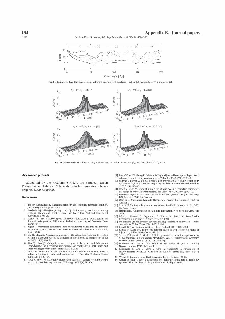
Acknowledgements
Supported by the Programme Alban, the European UnionProgramme of High Level Scholarships for Latin America, scholar-ship No. E06D101992CO.
References
[1] Booker JF. Dynamically loaded journal bearings—mobility method of solution.J Basic Eng 1965;87(3):537–46.
[2] Goodwin MJ, Nikolajsen JL, Ogrodnik PJ. Reciprocating machinery bearinganalysis: theory and practice. Proc Inst Mech Eng Part J—J Eng Tribol2003;217(6):409–26.
[3] Rasmussen BD. Variable speed hermetic reciprocating compressors fordomestic refrigerators. PhD thesis, Technical University of Denmark, Den-mark; 1997.
[4] Rigola J. Numerical simulation and experimental validation of hermeticreciprocating compressors. PhD thesis, Universidad Politecnica de Cataluna,Spain; 2002.
[5] Cho JR, Moon SJ. A numerical analysis of the interaction between the pistonoil film and the component deformation in a reciprocating compressor. TribolInt 2005;38(5):459–68.
[6] Kim TJ, Han JS. Comparison of the dynamic behavior and lubricationcharacteristics of a reciprocating compressor crankshaft in both finite andshort bearing models. Tribol Trans 2004;47(1):61–9.
[7] Santos IF, Nicoletti R, Scalabrin A. Feasibility of applying active lubrication toreduce vibration in industrial compressors. J Eng Gas Turbines Power2004;126(4):848–54.
[8] Stout K, Rowe W. Externally pressurized bearings—design for manufacturePart 1—journal bearing selection. Tribology 1974;7(3):98–106.
[9] Rowe W, Xu SX, Chong FS, Weston W. Hybrid journal bearings with particularreference to hole-entry configurations. Tribol Int 1982;15(6):339–48.
[10] Sharma S, Kumar V, Jain S, Sinhasan R, Subramanian M. A study of slot-entryhydrostatic/hybrid journal bearing using the finite element method. Tribol Int1999;32(4):185–96.
[11] Jadon V, Singh M. Study of supply cut-off and bearing geometric parameterson design of hybrid journal bearing. Ind Lubr Tribol 2007;59(2):92–102.
[12] Bremer H. Dynamik und regelung mechanischer systeme. Stuttgart Germany:B.G. Teubner; 1988 [in German].
[13] Ulbrich H. Maschinendynamik. Stuttgart, Germany: B.G. Teubner; 1996 [inGerman].
[14] Santos IF. Dinamica de sistemas mecanicos. Sao Paulo: Makron Books; 2001[in Portuguese].
[15] Hamrock BJ. Fundamentals of fluid film lubrication. New York: McGraw-Hill;1991.
[16] Frene J, Nicolas D, Degueurce B, Berthe D, Godet M. Lubrificationhydrodynamique. Paris: Editions Eyrolles; 1990.
[17] Mourelatos ZP. An efficient journal bearing lubrication analysis for enginecrankshafts. Tribol Trans 2001;44(3):351–8.
[18] Elrod HG. A cavitation algorithm. J Lubr Technol 1981;103(3):350–4.[19] Santos IF, Russo FH. Tilting-pad journal bearings with electronic radial oil
injection. J Tribol 1998;120(3):583–94.[20] Santos IF, Scalabrin A, Nicoletti R. Beitrag zur aktiven schmierungstheorie. In:
Schwingungen in Rotierenden Maschinen, vol. 5. Braunshweig, Germany:Vieweg Verlag; 2001. p. 21–30 [in German].
[21] Horikawa O, Sato K, Shimokohbe A. An active air journal bearing.Nanotechnology 1992;3(2):84–90.
[22] Mizumoto H, Arii S, Kami Y, Goto K, Yamamoto T, Kawamoto M.Active inherent restrictor for air-bearing spindles. Precis Eng 1996;19(2–3):141–7.
[23] Wendt JF. Computational fluid dynamics. Berlin: Springer; 1992.[24] Garcia de Jalon J, Bayo E. Kinematic and dynamic simulation of multibody
systems. The real-time challenge. New York: Springer; 1994.
ARTICLE IN PRESS
Fig. 14. Minimum fluid film thickness for different bearing configurations—hybrid lubrication (l ¼ 0:75 and �ab ¼ 0:2).
p [M
Pa]
z [mm]
p [M
Pa]
θc = 0°, Fb = 120 [N] θc = 90°, Fb = 132 [N]
θc = 270°, Fb = 120 2 [N]θc = 180°, Fb = 213 4 [N]
p [M
Pa]
p [M
Pa]
0 45 90 135 180 225 270 315
04
812
0
1
2
3
0
1
2
3
0
1
2
3
0
1
2
3
Θ [deg] z [mm]0 45 90 135 180 225 270 315
04
812
Θ [deg]
z [mm]0 45 90 135 180 225
270 315
04
812
Θ [deg] z [mm]0 45 90 135 180 225 270 315
048
12
Θ [deg]
Fig. 15. Pressure distribution, bearing with orifices located at Yo ¼ 180 (Pinj ¼ 2MPa, l ¼ 0:75, �ab ¼ 0:2).
E.A. Estupinan, I.F. Santos / Tribology International 42 (2009) 1478–14861486
134 Appendix B. Journal papers


DTU Mechanical Engineering
Section of Solid Mechanics
Technical University of Denmark
Nils Koppels Allé, Bld. 404
DK- 2800 Kgs. Lyngby
Denmark
Phone (+45) 45 25 42 50
Fax (+45) 45 93 14 75
www.mek.dtu.dk
ISBN: 978-87-89502-95-3
DCAMM
Danish Center for Applied Mathematics and Mechanics
Nils Koppels Allé, Bld. 404
DK-2800 Kgs. Lyngby
Denmark
Phone (+45) 4525 4250
Fax (+45) 4593 1475
www.dcamm.dk
ISSN: 0903-1685