FEASIBILITY STUDY TO IMPROVE TIDAL CIRCULATION IN WINDMILL COVE, OSTERVILLE, MASSACHUSETTS

by Trey Ruthven John Ramsey

FINAL REPORT – April 2002

Applied Coastal Research and Engineering, Inc. 766 Falmouth Road, Building A, Unit 1C Mashpee, MA 02649

1

1. INTRODUCTION The purpose of this study was to determine whether it was possible to improve tidal circulation and the associated water quality within Windmill Cove. Due to the relatively poor water quality conditions within both the North and South Coves, potential hydraulic connections to enhance water movement were explored. A variety of culverts connecting South Cove and North Cove were evaluated; however, the alternatives selected for analysis were limited to options that were considered feasible from both an engineering and environmental perspective. First, it was determined that the existing causeway connecting the two islands was to remain in its existing form (width and elevation). In addition, it was concluded that potential options for improving tidal circulation should involve relatively minor excavation of the existing marsh plain (i.e. cutting small channels between the edge of the seaward edge of the marsh and the causeway to service the culverts). Alterations to the causeway dimensions and/or major excavation of the marsh plain potentially could have large impacts to the existing marsh system; therefore, options that required these types of alterations (e.g. removing the causeway and constructing a bridge) were removed from further consideration. Initially, a field study was designed to determine marsh health, as well as to determine the various physical properties needed to parameterize the hydrodynamic model. Based on the results of the initial model simulations, detailed biological analyses of the marsh system were deemed unnecessary. In general, the hydrodynamic modeling indicated that reasonably-sized culverts would not appreciably improve circulation within the two Coves. A more detailed evaluation of the culvert alternatives influence on tidal exchange is presented in Section 3.

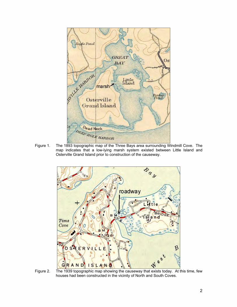
1.1 Historical Conditions Construction of the Osterville Grand Island causeway prevented overwash and/or tidal exchange between North Windmill Cove (North Cove) and South Windmill Cove (South Cove). Historically, the low-lying area between Little Island and Osterville Grand Island (Grand Island) likely allowed tidal waters to propagate from West Bay into North Bay. The 1893 topographic map shown in Figure 1 shows the marsh area between Little Island and Grand Island, as well as the single-inlet Three Bays estuarine system. Although tidal exchange between West Bay (not labeled) and North Bay (labeled Great Bay on Figure 1) was not restricted by either the Little Island Bridge or the causeway, the West Bay Cut did not exist at the time. Therefore, tidal waters needed to travel through the Cotuit Bay entrance (labeled Osterville Harbor on Figure 1) to reach Windmill Cove. Following construction of the Little Island Bridge and the causeway connecting Little Island to Grand Island in the early 1900s, tidal flow between North and South Coves no longer occurred. However, the West Bay Cut was developed, and the distance tidal water needed to travel from Nantucket Sound to flush the Coves was reduced. Overall, the West Bay Cut provided better regional circulation for West Bay. Figure 2 depicts the alterations made to the Windmill Cove area between 1893 and 1939. Construction of the causeway bifurcated the low-lying marsh system between Little and Grand Islands. At the time of this map, few houses existed on Grand Island and the majority of the marsh system existed around South Cove.

2

Figure 1. The 1893 topographic map of the Three Bays area surrounding Windmill Cove. The

map indicates that a low-lying marsh system existed between Little Island and Osterville Grand Island prior to construction of the causeway.

Figure 2. The 1939 topographic map showing the causeway that exists today. At this time, few

houses had been constructed in the vicinity of North and South Coves.

3

1.2 Existing Conditions Development of both Little and Grand Islands over the past 50 years has reduced the Windmill Cove marsh area, especially surrounding South Cove. Figure 3 shows the 1994 aerial photograph, indicating the area along the northeast section of South Cove that had been filled for house construction. In addition, the photograph indicates several docks in North Cove, as well as a widened marsh channel along the eastern edge of South Cove for small boat navigation. The alterations to both the upland and the marsh system during the past 50 years have resulted in a reduction in marsh area around Windmill Cove. Based on initial observations of the marsh plain, the boundaries between low and high salt marsh appear to be primarily controlled by subtle elevation changes across the marsh. The marsh plain is relatively narrow, where rising tides in either North Cove or South Cove can easily propagate across the marsh surface. In addition, the marsh plant density does not appear to significantly inhibit sheet flow across the marsh plain. Typical of most marshes, the height and density of marsh vegetation is greatest along the edge of channels (mosquito ditches) that service the marsh. Within the Three Bays estuarine system, small sub-embayments (e.g. North and South Coves) typically exhibit slightly lower water quality than the larger embayments (e.g. North Bay). This reduction in overall water quality is generally attributed to the relatively poor flushing condition of these sub-embayments, and is seen in water column monitoring results as increased total nitrogen levels, higher chlorophyll-a levels, and decreased dissolved oxygen levels. Based on monitoring results within North Cove (2 years of data) and South Cove (1 year of data), the eutrophication index developed for these two sub-embayments indicates a slightly lower quality than the source waters, where the source waters for North Cove is North Bay and the source waters for South Cove is West Bay. Due to the relatively poor water quality within the two Coves, potential tidal circulation improvements were sought. By hydraulically connecting North Cove to South Cove, an increase in tidal flushing could be driven by the elevation differences that exist between the Coves. If this change in tidal flushing was deemed significant, the lower quality water contained within the Coves would be diluted with higher quality Bay water.

4

Figure 3. The 1994 aerial photograph showing the series of docks constructed around North

Cove, the filled area in the northeast portion of the South Cove marsh, and the widened small boat channel servicing this area.

5

2. DATA COLLECTION AND ANALYSIS

The field data collection portion of this study was performed to characterize the physical properties of the North and South Cove within Three Bays Estuary. Bathymetry was collected throughout the system so that it could be accurately represented as a computer hydrodynamic model. In addition to the bathymetry, tide data were also collected at two locations in the system, to run the circulation model with real tides, and also to calibrate and verify its performance.

2.1 Bathymetry Data Collection

Bathymetry in the North and South Cove was collected during March 2002. The survey employed a bottom tracking Acoustic Doppler Current Profiler (ADCP) mounted on a survey vessel. Positioning data were collected using a differential GPS. The survey was designed to capture the bathymetric features of the coves, the east-west transects were space at 150 ft with the cross transects spaced more closely to capture detail within channel and around the marsh planes. The actual survey paths are shown in Figure 4. The red makers represent the data points collected in the ADCP survey, the blue markers represents marsh plain data collected by Cape Surv. The resulting bathymetric surface created by interpolating the data to a finite element mesh is shown in Figure 5. All bathymetry was tide corrected, and referenced to the North Geodetic Vertical Datum (NGVD 29).

Figure 4. Transects from the bathymetry survey of the North and South Cove.

6

Results from the survey show that the deepest water is located within the North Cove along the channel and in the depression in the middle of cove. The water depths in the channel vary from -6.5 ft NGVD29 to the deepest point -11.3 ft NGVD29. The South Cove is relatively shallow compared to the North Cove. Water depths average approximately -2.0 ft NGVD29. The deepest water is located at the southern end of the cove at the entrance to the West Bay, with a water depth of -4.02 ft NGVD29.

Figure 5. Bathymetry data interpolated to the finite element mesh used with the RMA-2

hydrodynamic model. Contours represent the bottom elevation relative to NGVD 29. Tide gage locations are shown.

2.2 Tide Data Collection and Analysis

Tide data records were collected at two stations in the Three Bays estuary system. The first was located on the western edge of the North Cove, the second was on the western edge of the South Cove. The locations of the stations are represented by the black dots in Figure 5. The Temperature Depth Recorders (TDR) used to record the tide data were deployed for a 65-day period between January 4, 2002 and March 10, 2002. The elevation of each gauge was surveyed relative to NGVD 29. Each tide record was used to as the open boundary condition of the hydrodynamic model.

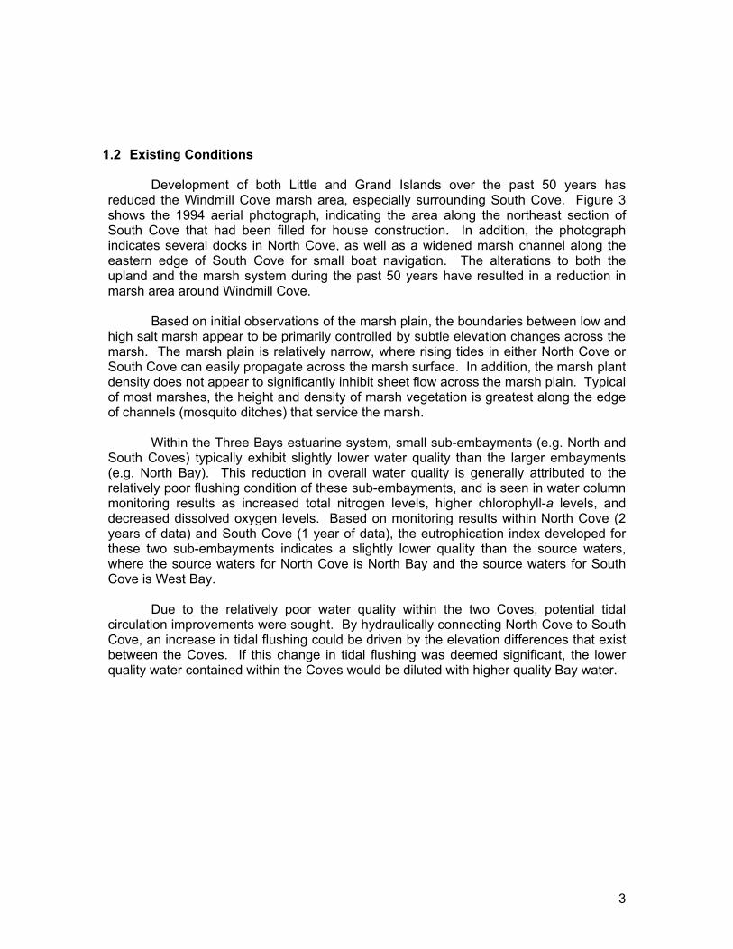
Plots of the tide data from the three gauges are shown in Figure 6, for the entire 65-day deployment. The spring-to-neap variations in tide range are not easily

7

discernable in these plots, likely due to the influence of wind on the water levels within the bay. Depending on the speed and direction of the wind, large differences in the water level can be seen from the normal tidal variations in water surface elevation. A visual comparison between tide elevations at the two stations shows that there is only a minor variation in the tide range between the South Cove and the North Cove. The relatively small tidal attenuation between West Bay (servicing the South Cove) and North Bay (servicing the North Cove) limits the amount of tide range variabity observed between the two Coves.

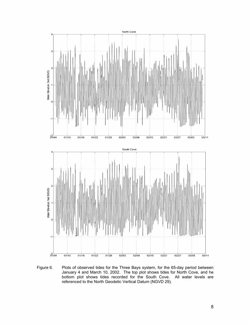
To better quantify the changes to the tide from the inlet to inside the system, the standard tide datums were computed from the 65-day records. These datums are presented in Table 1. For most NOAA tide stations, these datums are computed using 19 years of tide data, the definition of a tidal epoch. For this study, a significantly shorter time span of data was available, however, these datums still provide a useful comparison of tidal dynamics within the system. The Mean Higher High (MHH) and Mean Lower Low (MLL) levels represent the mean of the daily highest and lowest water levels. The Mean High Water (MHW) and Mean Low Water (MLW) levels represent the mean of all the high and low tides of a record, respectively. The Mean Tide Level (MTL) is simply the mean of MHW and MLW.

The low water datums (MLW, MLLW, and minimum tide) for the South Cove are

higher than the those for the North Cove due the placement of the tide gage. Examination of the tide record for the South Cove gauge revealed that no water surface elevations below -1.0 ft NGVD. Water levels below -1.0 ft NGVD were not recorded by the gage because water level actually dropped below the pressure sensor at this location. For future tide measurements in South Cove, the gage should be relocated to deeper water to ensure tides are recorded even at extreme low water events. The absence of data from below -1.0 ft NGVD artificially increases the water level datums for MLW, MLLW, and minimum tide. However, comparing the differences between the North and South Cove reveals that the differences are not significant over this time period.

Table 1. Tide datums computed from 65-day records collected at North and South Cove. Datum elevations are given relative to NGVD 29.

Tide Datum North Cove (feet)

South Cove (feet)

Maximum Tide 3.6 3.5 MHHW 2.6 2.7 MHW 2.2 2.2 MTL 0.8 0.9 MLW -0.7 -0.5 MLLW -1.0 -0.8 Minimum Tide -1.5 -1.0

8

Figure 6. Plots of observed tides for the Three Bays system, for the 65-day period between

January 4 and March 10, 2002. The top plot shows tides for North Cove, and he bottom plot shows tides recorded for the South Cove. All water levels are referenced to the North Geodetic Vertical Datum (NGVD 29).

9

A harmonic analysis was performed on the time series from each gage location. Harmonic analysis is a mathematical procedure that fits sine–curves of known frequency to the measured signal. The amplitudes and phase of 23 known tidal constituents result from this procedure. A more complete description of this analysis procedure is presented in the Appendix. In general, the sine-curves are developed based on the various gravitational forces influencing the tides (e.g. the moon and sun). The familiar twice-a-day lunar tide, known as the M2, is the strongest contributor to the signal with an amplitude of 1.26 at the South Cove.

As the tide propagates into the upper reaches of an estuary the elevation of the tide usually varies. This is due to the effects of frictional damping on tide. Frictional damping is usually evident as a decrease in the amplitude of M2 constituent. Usually, a portion of the energy lost from the M2 tide is transferred to higher harmonics (i.e., the M4 and M6), and is observed as an increase in amplitude of these constituents over the length of an estuary. However, within the Three Bays estuary, the Coves are located so closely to one another that a clear reduction in the tidal signal is not evident here.

Phase delay is another indication of tidal damping, and results with a later high

tide at inland locations. The greater the frictional effects, the longer the delay between locations. The phase delay of the M2 tide between the South Cove and the gage in the North Cove was determined to be 3.56 minutes, by the harmonic analysis. This shows the short distance and the lack of large obstructions through the channel connecting West and North Bays results in very minor changes to the tidal signal as it propagates into the Coves.

10

3. HYDRODYNAMIC MODELING For the modeling of the culvert between the North and South Coves of the Three Bays Estuary, Applied Coastal utilized a state-of-the-art computer model to evaluate tidal circulation and flushing in these systems. The particular model employed was the RMA-2 model developed by Resource Management Associates (King, 1990). It is a two-dimensional, depth-averaged finite element model, capable of simulating transient hydrodynamics. The model is widely accepted and tested for analyses of estuaries or rivers.

3.1 Model Theory In its original form, RMA-2 was developed by William Norton and Ian King under contract with the U.S. Army Corps of Engineers (Norton et al., 1973). Further development included the introduction of one-dimensional elements, state-of-the-art pre- and post-processing data programs, and the use of elements with curved borders. Recently, the graphic pre- and post-processing routines were updated by a Brigham Young University through a package called the Surface water Modeling System or SMS (BYU, 1998). Graphics generated in support of this report primarily were generated within the SMS modeling package. RMA-2 is a finite element model designed for simulating one- and two-dimensional depth-averaged hydrodynamic systems. The dependent variables are velocity and water depth, and the equations solved are the depth-averaged Navier Stokes equations. Reynolds assumptions are incorporated as an eddy viscosity effect to represent turbulent energy losses. Other terms in the governing equations permit friction losses (approximated either by a Chezy or Manning formulation), Coriolis effects, and surface wind stresses. All the coefficients associated with these terms may vary from element to element. The model utilizes quadrilaterals and triangles to represent the prototype system. Element boundaries may either be curved or straight. The time dependence of the governing equations is incorporated within the solution technique needed to solve the set of simultaneous equations. This technique is implicit; therefore, unconditionally stable. Once the equations are solved, corrections to the initial estimate of velocity and water elevation are employed, and the equations are re-solved until the convergence criteria is met.

3.2 Model Setup There are three main steps required to implement RMA-2: • Grid generation • Boundary condition specification • Calibration The extent of each finite element grid was generated using 1994 digital aerial photographs from the MassGIS online orthophoto database. A time-varying water surface elevation boundary condition (measured tide) was specified at the entrance of each system based on the tide gauge data collected in the North and South Coves. Once the grid and boundary conditions were set, the model was calibrated to ensure

11

accurate predictions of tidal flushing. Various friction and eddy viscosity coefficients were adjusted, through several model calibration simulations for each system, to obtain agreement between measured and modeled tides. The calibrated model provides the requisite information for future detailed water quality modeling.

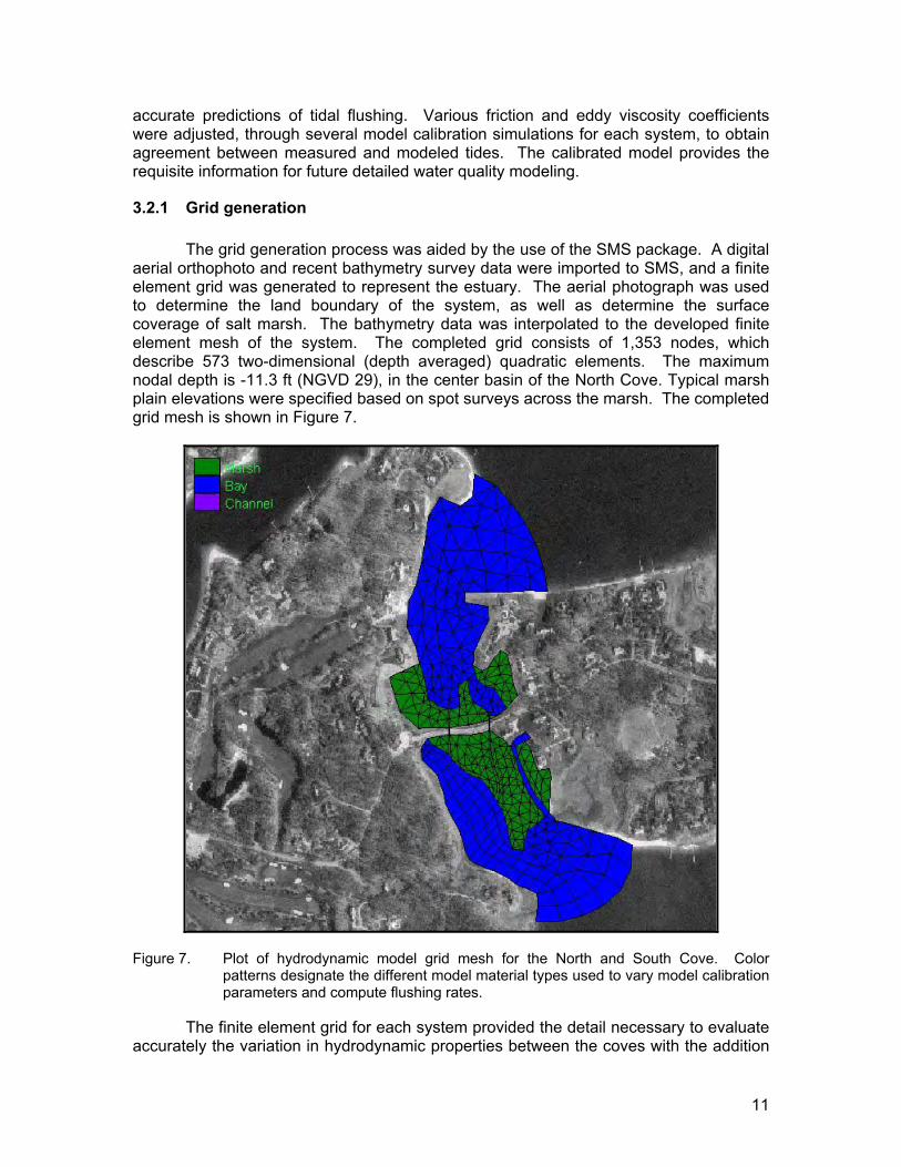
3.2.1 Grid generation The grid generation process was aided by the use of the SMS package. A digital aerial orthophoto and recent bathymetry survey data were imported to SMS, and a finite element grid was generated to represent the estuary. The aerial photograph was used to determine the land boundary of the system, as well as determine the surface coverage of salt marsh. The bathymetry data was interpolated to the developed finite element mesh of the system. The completed grid consists of 1,353 nodes, which describe 573 two-dimensional (depth averaged) quadratic elements. The maximum nodal depth is -11.3 ft (NGVD 29), in the center basin of the North Cove. Typical marsh plain elevations were specified based on spot surveys across the marsh. The completed grid mesh is shown in Figure 7.

Figure 7. Plot of hydrodynamic model grid mesh for the North and South Cove. Color

patterns designate the different model material types used to vary model calibration parameters and compute flushing rates.

The finite element grid for each system provided the detail necessary to evaluate

accurately the variation in hydrodynamic properties between the coves with the addition

12

of culverts to pass water between them. The SMS grid generation program was used to develop quadrilateral and triangular two-dimensional elements throughout the estuary. Channels were manually added to the marsh planes during the alternatives analysis to assist in the transition water through the culverts between the coves. Grid resolution was governed by two factors: 1) expected flow patterns, and 2) the bathymetric variability of the system. Relatively fine grid resolution was employed where complex flow patterns were expected. For example, smaller node spacing in marsh and marsh channels was designed to provide a more detailed analysis in these regions of rapidly varying flow. Widely spaced nodes were often employed in areas where flow patterns are not likely to change dramatically, such as in the coves. Appropriate implementation of wider node spacing and larger elements reduced computer run time with no sacrifice of accuracy.

3.2.2 Boundary condition specification Two types of boundary conditions were employed for the RMA-2 model of the Back River system: 1) "slip" boundaries, and 2) tidal elevation boundaries. All of the elements with land borders have "slip" boundary conditions, where the direction of flow was constrained shore-parallel. The model generated all internal boundary conditions from the governing conservation equations. A tidal boundary condition was specified along the seaward edges of the North and South Coves. TDR measurements provided the required data. Dynamic (time-varying) model simulations specified a new water surface elevation every model time step (10 minutes).

3.2.3 Calibration After developing the finite element grids, and specifying boundary conditions, the model for the coves was calibrated. The calibration procedure ensures that the model predicts accurately what was observed in nature during the field measurement program. Numerous model simulations are required for an estuary model, specifying a range of friction and eddy viscosity coefficients, to calibrate the model. Calibration of the hydrodynamic model required a close match between the modeled and measured tides in each cove where tides were measured (i.e., from the TDR deployments). The model was calibrated using a visual reference to check the agreement between modeled and measured tides. The coefficients utilized for model calibration were based on previous experience with other estuarine/salt marsh systems with similar tidal characteristics.

3.2.3.a Friction coefficients Friction inhibits flow along the bottom of estuary channels or other flow regions where velocities are relatively high. Friction is a measure of the channel roughness, and can cause both significant amplitude damping and phase delay of the tidal signal. Friction is approximated in RMA-2 as a Manning coefficient, and is applied to grid areas by user specified material types. Initially, Manning's friction coefficients between 0.02 and 0.07 were specified for all element material types. These values correspond to typical Manning's coefficients determined experimentally in smooth earth-lined channels

13

with no weeds (low friction) to winding channels and marsh plains with higher friction (Henderson, 1966). To improve model accuracy, friction coefficients were varied throughout the model domain. First, the Manning’s coefficients were matched to bottom type. For example, lower friction coefficients were specified for the smooth bottom of the Coves, versus the vegetated marsh surface, which provides greater flow resistance. Final model calibration runs incorporated various specific values for Manning's friction coefficients, depending upon flow damping characteristics of separate regions within each estuary. Manning's values for different bottom types were initially selected based ranges provided by the Civil Engineering Reference Manual (Lindeburg, 1992), and values were incrementally changed when necessary to obtain a close match between measured and modeled tides. Final calibrated friction coefficients are summarized in the Table 2.

Table 2. Manning’s Roughness coefficients used in simulations of modeled embayments. These embayment delineations correspond to the material type areas shown in Figure 6.

System Embayment Bottom Friction

Bays 0.025 Marsh 0.075

3.2.3.b Turbulent exchange coefficients

Turbulent exchange coefficients approximate energy losses due to internal friction between fluid particles. The significance of turbulent energy losses increases where flow is swifter, such as inlets and bridge constrictions. According to King (1990), these values are proportional to element dimensions (numerical effects) and flow velocities (physics). In most cases, the modeled systems were relatively insensitive to turbulent exchange coefficients because there were no regions of strong turbulent flow. Typically, model turbulence coefficients were set between 30 and 50 lb-sec/ft2.

3.2.3.c Marsh porosity processes

Modeled hydrodynamics were complicated by wetting/drying cycles on the marsh plain included in the model. Cyclically wet/dry areas of the marsh will tend to store waters as the tide begins to ebb and then slowly release water as the water level drops within the creeks and channels. This store-and-release characteristic of these marsh regions was partially responsible for the distortion of the tidal signal, and the elongation of the ebb phase of the tide. On the flood phase, water rises within the channels and creeks initially until water surface elevation reaches the marsh plain, when at this point the water level remains nearly constant as water ‘fans’ out over the marsh surface. The rapid flooding of the marsh surface corresponds to a flattening out of the tide curve approaching high water. Marsh porosity is a feature of the RMA-2 model that permits the modeling of hydrodynamics in marshes. This model feature essentially simulates the

14

store-and-release capability of the marsh plain by allowing grid elements to transition gradually between wet and dry states. This technique allows RMA-2 to change the ability of an element to hold water, like squeezing a sponge. The marsh porosity feature of RMA-2 is typically utilized in estuarine systems where the marsh plain has a significant impact on the hydrodynamics of a system.

3.2.3.d Comparison of modeled tides and measured tide data

A visual calibration was used for the modeled tidal hydrodynamics in the coves. Generally a harmonic analysis would be done to calibrate the modeled tides against gage measurements throughout the estuary system. The lack of restrictions in Three Bays Estuary does not produce a significant amount of tidal damping between the North and South Cove. Also, the gauge records were used to drive the tidal boundary conditions. Therefore, a harmonic analysis of the water levels would not give clear indication of the calibration in this case since the distance is relatively short and there are no definable restrictions between the boundary and the gage station.

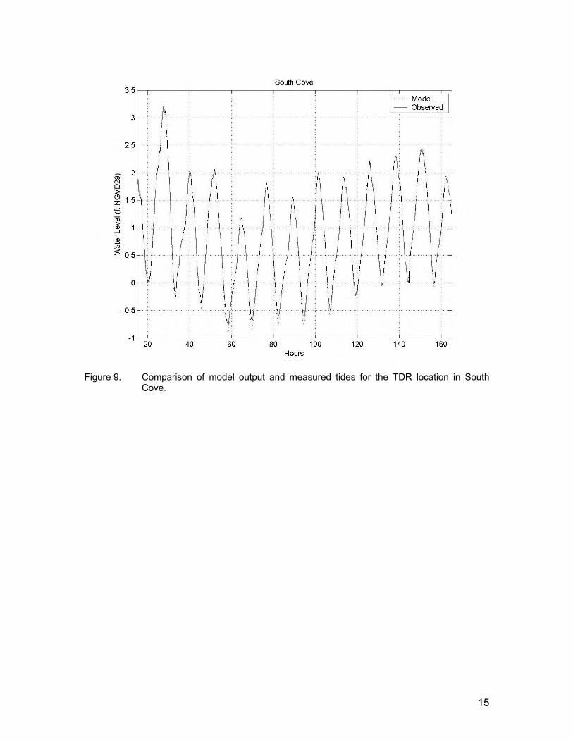
A visual calibration of the model was achieved using the aforementioned values

for friction and turbulent exchange. Figures 8 and 9 illustrate the six-day calibration simulation for the North and South Cove. Modeled (solid line) and measured (dotted line) tides are illustrated at each model location with a corresponding TDR. The graphs indicated good agreement between the model and data.

Figure 8. Comparison of model output and measured tides for the TDR location in North

Cove.

15

Figure 9. Comparison of model output and measured tides for the TDR location in South

Cove.

16

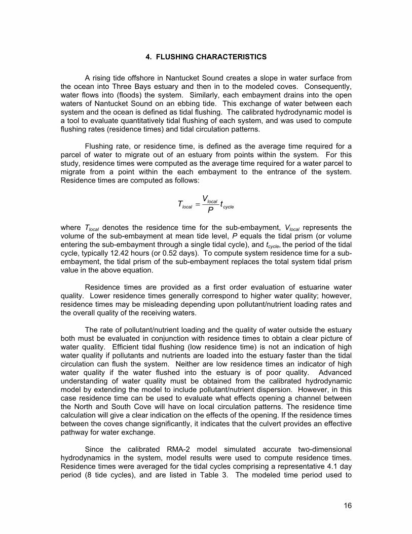
4. FLUSHING CHARACTERISTICS A rising tide offshore in Nantucket Sound creates a slope in water surface from the ocean into Three Bays estuary and then in to the modeled coves. Consequently, water flows into (floods) the system. Similarly, each embayment drains into the open waters of Nantucket Sound on an ebbing tide. This exchange of water between each system and the ocean is defined as tidal flushing. The calibrated hydrodynamic model is a tool to evaluate quantitatively tidal flushing of each system, and was used to compute flushing rates (residence times) and tidal circulation patterns. Flushing rate, or residence time, is defined as the average time required for a parcel of water to migrate out of an estuary from points within the system. For this study, residence times were computed as the average time required for a water parcel to migrate from a point within the each embayment to the entrance of the system. Residence times are computed as follows:

cyclelocal

local tP

VT =

where Tlocal denotes the residence time for the sub-embayment, Vlocal represents the volume of the sub-embayment at mean tide level, P equals the tidal prism (or volume entering the sub-embayment through a single tidal cycle), and tcycle, the period of the tidal cycle, typically 12.42 hours (or 0.52 days). To compute system residence time for a sub-embayment, the tidal prism of the sub-embayment replaces the total system tidal prism value in the above equation. Residence times are provided as a first order evaluation of estuarine water quality. Lower residence times generally correspond to higher water quality; however, residence times may be misleading depending upon pollutant/nutrient loading rates and the overall quality of the receiving waters. The rate of pollutant/nutrient loading and the quality of water outside the estuary both must be evaluated in conjunction with residence times to obtain a clear picture of water quality. Efficient tidal flushing (low residence time) is not an indication of high water quality if pollutants and nutrients are loaded into the estuary faster than the tidal circulation can flush the system. Neither are low residence times an indicator of high water quality if the water flushed into the estuary is of poor quality. Advanced understanding of water quality must be obtained from the calibrated hydrodynamic model by extending the model to include pollutant/nutrient dispersion. However, in this case residence time can be used to evaluate what effects opening a channel between the North and South Cove will have on local circulation patterns. The residence time calculation will give a clear indication on the effects of the opening. If the residence times between the coves change significantly, it indicates that the culvert provides an effective pathway for water exchange. Since the calibrated RMA-2 model simulated accurate two-dimensional hydrodynamics in the system, model results were used to compute residence times. Residence times were averaged for the tidal cycles comprising a representative 4.1 day period (8 tide cycles), and are listed in Table 3. The modeled time period used to

17

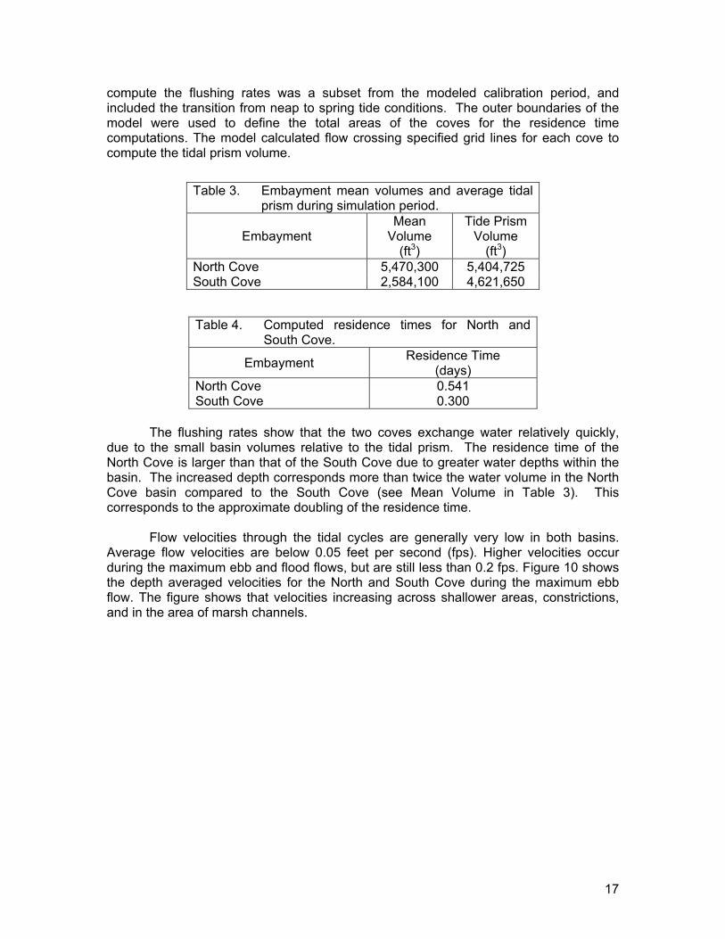
compute the flushing rates was a subset from the modeled calibration period, and included the transition from neap to spring tide conditions. The outer boundaries of the model were used to define the total areas of the coves for the residence time computations. The model calculated flow crossing specified grid lines for each cove to compute the tidal prism volume.

Table 3. Embayment mean volumes and average tidal prism during simulation period.

Embayment Mean

Volume (ft3)

Tide Prism Volume

(ft3) North Cove 5,470,300 5,404,725 South Cove 2,584,100 4,621,650

The flushing rates show that the two coves exchange water relatively quickly,

due to the small basin volumes relative to the tidal prism. The residence time of the North Cove is larger than that of the South Cove due to greater water depths within the basin. The increased depth corresponds more than twice the water volume in the North Cove basin compared to the South Cove (see Mean Volume in Table 3). This corresponds to the approximate doubling of the residence time.

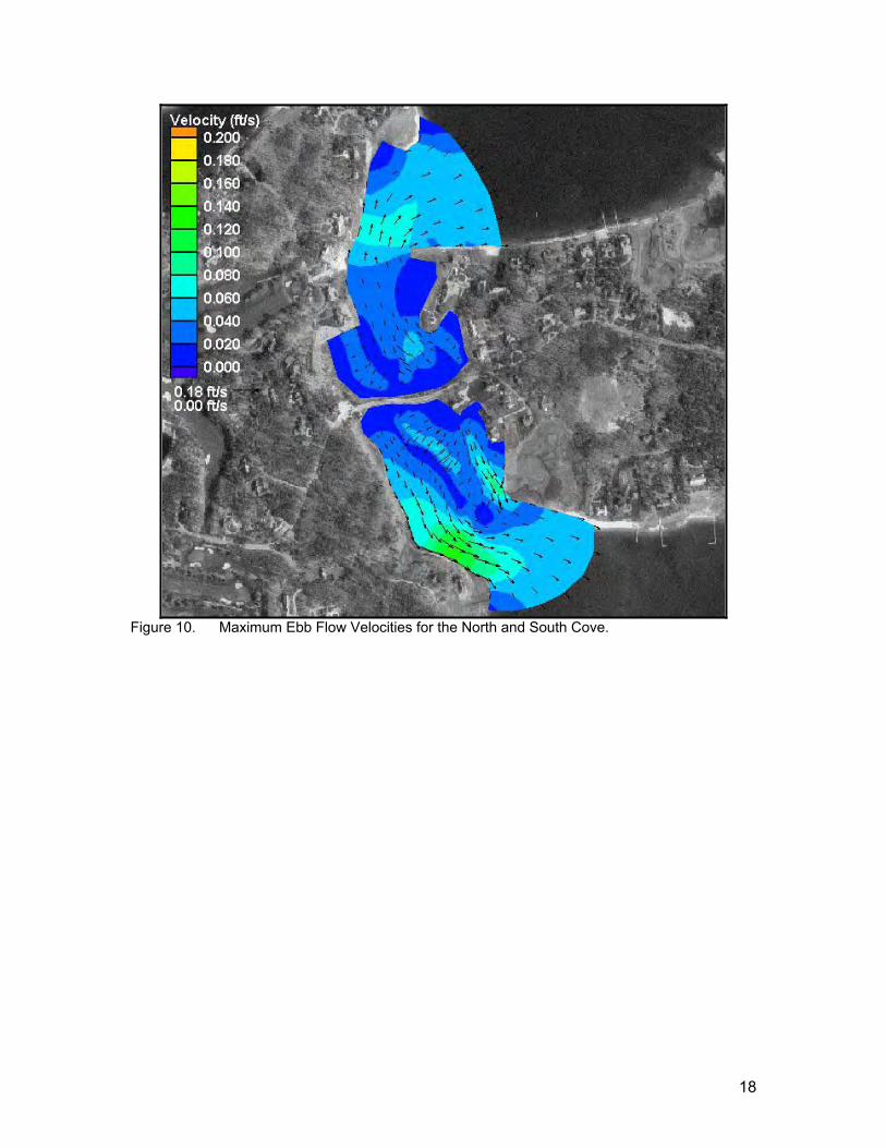
Flow velocities through the tidal cycles are generally very low in both basins.

Average flow velocities are below 0.05 feet per second (fps). Higher velocities occur during the maximum ebb and flood flows, but are still less than 0.2 fps. Figure 10 shows the depth averaged velocities for the North and South Cove during the maximum ebb flow. The figure shows that velocities increasing across shallower areas, constrictions, and in the area of marsh channels.

Table 4. Computed residence times for North and South Cove.

Embayment Residence Time (days)

North Cove 0.541 South Cove 0.300

18

Figure 10. Maximum Ebb Flow Velocities for the North and South Cove.

19

5. FEASIBILITY

The goal of this study was to examine alternatives for improving the circulation characteristics of the North and South Cove. Four alternatives where developed for creating openings in the roadway/causeway between Osterville Grand Island and Little Island to allow water to move directly between the coves. The hydrodynamic model was used to evaluate the impacts on circulation and residence times with each of the different alternatives.

5.1 Alternatives

The four alternatives consist of different culvert and channel configurations to

create the openings between the North and South Coves. Culverts where chosen because the roadway is the only access for residents of Osterville Grand Island. The use of culverts would allow for a staged construction sequence to provide continual access to the island. One of the initial alternatives was a bridge, since it would provide a larger opening between the coves. However, the construction of the bridge would require the complete removal of the roadway prior to bridge construction. This would limit access to the island for a period of six months to a year. In addition, the channel linking North Cove and South Cove would require substantial excavation of the salt marsh resources. Due to the unacceptable limitations associated with potential environmental impacts and loss of island access during construction, the bridge option was discarded.

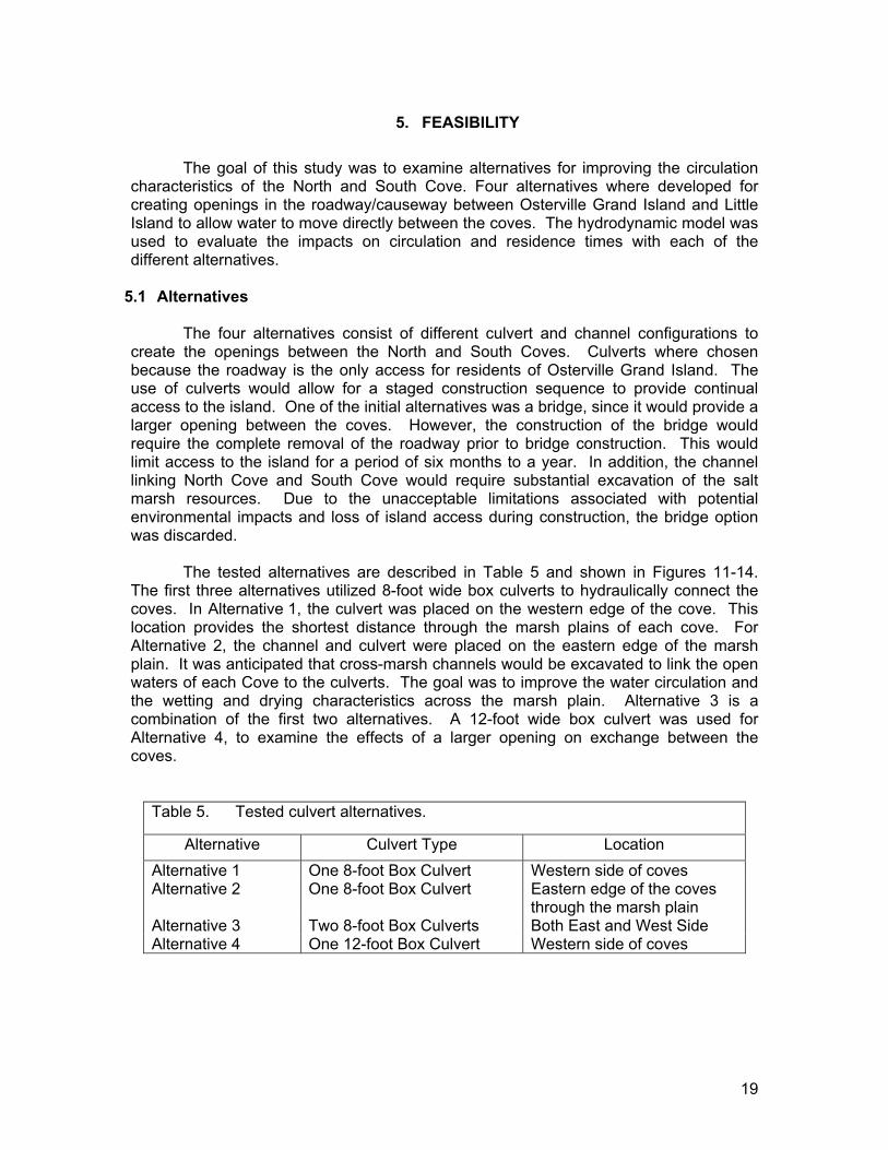
The tested alternatives are described in Table 5 and shown in Figures 11-14.

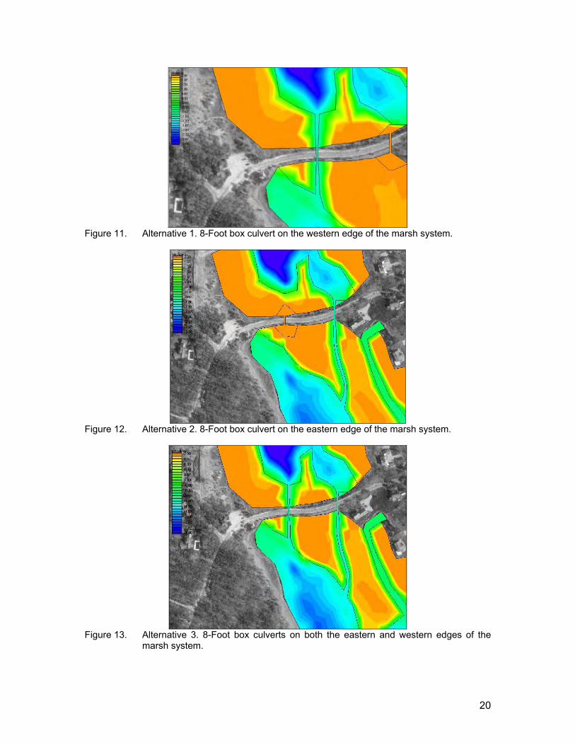
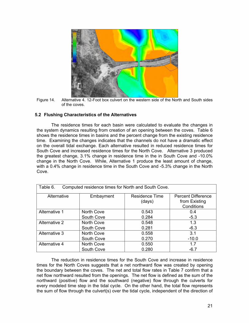
The first three alternatives utilized 8-foot wide box culverts to hydraulically connect the coves. In Alternative 1, the culvert was placed on the western edge of the cove. This location provides the shortest distance through the marsh plains of each cove. For Alternative 2, the channel and culvert were placed on the eastern edge of the marsh plain. It was anticipated that cross-marsh channels would be excavated to link the open waters of each Cove to the culverts. The goal was to improve the water circulation and the wetting and drying characteristics across the marsh plain. Alternative 3 is a combination of the first two alternatives. A 12-foot wide box culvert was used for Alternative 4, to examine the effects of a larger opening on exchange between the coves.

Table 5. Tested culvert alternatives.

Alternative Culvert Type Location Alternative 1 One 8-foot Box Culvert Western side of coves Alternative 2 One 8-foot Box Culvert Eastern edge of the coves

through the marsh plain Alternative 3 Two 8-foot Box Culverts Both East and West Side Alternative 4 One 12-foot Box Culvert Western side of coves

20

Figure 11. Alternative 1. 8-Foot box culvert on the western edge of the marsh system.

Figure 12. Alternative 2. 8-Foot box culvert on the eastern edge of the marsh system.

Figure 13. Alternative 3. 8-Foot box culverts on both the eastern and western edges of the

marsh system.

21

Figure 14. Alternative 4. 12-Foot box culvert on the western side of the North and South sides

of the coves.

5.2 Flushing Characteristics of the Alternatives

The residence times for each basin were calculated to evaluate the changes in the system dynamics resulting from creation of an opening between the coves. Table 6 shows the residence times in basins and the percent change from the existing residence time. Examining the changes indicates that the channels do not have a dramatic effect on the overall tidal exchange. Each alternative resulted in reduced residence times for South Cove and increased residence times for the North Cove. Alternative 3 produced the greatest change, 3.1% change in residence time in the in South Cove and -10.0% change in the North Cove. While, Alternative 1 produce the least amount of change, with a 0.4% change in residence time in the South Cove and -5.3% change in the North Cove.

Table 6. Computed residence times for North and South Cove.

Alternative Embayment Residence Time (days)

Percent Difference from Existing Conditions

North Cove 0.543 0.4 Alternative 1 South Cove 0.284 -5.3 North Cove 0.548 1.3 Alternative 2 South Cove 0.281 -6.3 North Cove 0.558 3.1 Alternative 3 South Cove 0.270 -10.0 North Cove 0.550 1.7 Alternative 4 South Cove 0.280 -6.7

The reduction in residence times for the South Cove and increase in residence

times for the North Coves suggests that a net northward flow was created by opening the boundary between the coves. The net and total flow rates in Table 7 confirm that a net flow northward resulted from the openings. The net flow is defined as the sum of the northward (positive) flow and the southward (negative) flow through the culverts for every modeled time step in the tidal cycle. On the other hand, the total flow represents the sum of flow through the culvert(s) over the tidal cycle, independent of the direction of

22

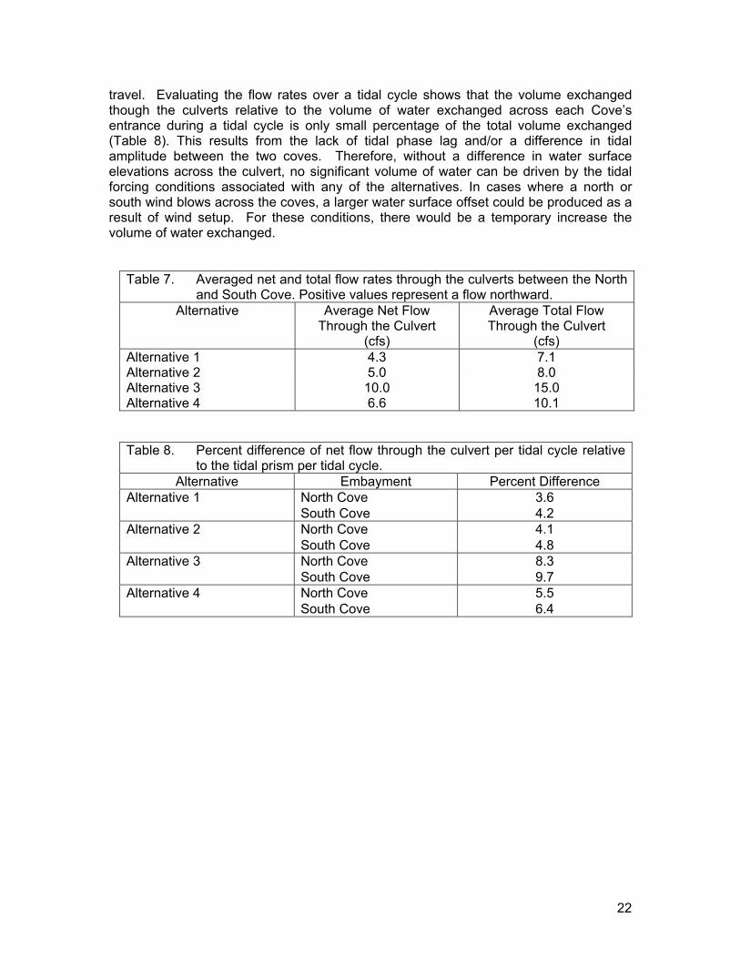
travel. Evaluating the flow rates over a tidal cycle shows that the volume exchanged though the culverts relative to the volume of water exchanged across each Cove’s entrance during a tidal cycle is only small percentage of the total volume exchanged (Table 8). This results from the lack of tidal phase lag and/or a difference in tidal amplitude between the two coves. Therefore, without a difference in water surface elevations across the culvert, no significant volume of water can be driven by the tidal forcing conditions associated with any of the alternatives. In cases where a north or south wind blows across the coves, a larger water surface offset could be produced as a result of wind setup. For these conditions, there would be a temporary increase the volume of water exchanged.

Table 7. Averaged net and total flow rates through the culverts between the North and South Cove. Positive values represent a flow northward.

Alternative Average Net Flow Through the Culvert

(cfs)

Average Total Flow Through the Culvert

(cfs) Alternative 1 4.3 7.1 Alternative 2 5.0 8.0 Alternative 3 10.0 15.0 Alternative 4 6.6 10.1

Table 8. Percent difference of net flow through the culvert per tidal cycle relative to the tidal prism per tidal cycle.

Alternative Embayment Percent Difference North Cove 3.6 Alternative 1 South Cove 4.2 North Cove 4.1 Alternative 2 South Cove 4.8 North Cove 8.3 Alternative 3 South Cove 9.7 North Cove 5.5 Alternative 4 South Cove 6.4

23

6. CONCLUSIONS Construction of the Osterville Grand Island causeway in the early 1900’s prevented overwash and/or tidal exchange between North Windmill Cove (North Cove) and South Windmill Cove (South Cove). Prior to the construction of the causeway, the low-lying area between Little Island and Osterville Grand Island (Grand Island) likely allowed tidal waters to propagate from West Bay into North Bay. Increased housing development on both Little and Grand Islands over the past 50 years has reduced the Windmill Cove marsh area, especially surrounding South Cove. Based on site observations of the marsh plain in March 2002, the boundaries between low and high salt marsh appear to be primarily controlled by subtle elevation changes across the marsh. The marsh plain is relatively narrow, where rising tides in either North Cove or South Cove can easily propagate across the marsh surface. In addition, the marsh plant density does not appear to significantly inhibit sheet flow across the marsh plain. Typical of most marshes, the height and density of marsh vegetation is greatest along the edge of channels (mosquito ditches) that service the marsh. Within the Three Bays estuarine system, small sub-embayments (e.g. North and South Coves) typically exhibit slightly lower water quality than the larger embayments (e.g. North Bay). This reduction in overall water quality is generally attributed to the relatively poor flushing condition of these sub-embayments, and is seen in water column monitoring results as increased total nitrogen levels, higher chlorophyll-a levels, and decreased dissolved oxygen levels. Based on monitoring results within North Cove (2 years of data) and South Cove (1 year of data), the eutrophication index developed for these two sub-embayments indicates a slightly lower quality than the source waters, where the source waters for North Cove is North Bay and the source waters for South Cove is West Bay. Due to this relatively poor water quality within the two Coves, potential tidal circulation improvements were sought. By hydraulically connecting North Cove to South Cove, an increase in tidal flushing could be driven by the elevation differences that exist between the Coves. If this change in tidal flushing was deemed significant, the lower quality water contained within the Coves would be diluted with higher quality Bay water. Two-dimensional hydrodynamic modeling of North and South Coves was conducted. In addition, four culvert alternatives were explored in the context of the model to determine what level of circulation improvements would occur as a result of hydraulically connecting the Coves. Input to the model consisted of tide-corrected bathymetric data measured in March 2002, as well as a two-month tide record in both North Cove and South Cove. Based on the tidal data collected, it was found that the tidal amplitude was nearly identical within each of the Coves. In addition, the phase lag between South Cove and North Cove is only about 3.5 minutes, where the tide reaches South Cove slightly before it reaches North Cove. This lack of tidal attenuation is due to the relatively efficient existing channel system between West Bay and North Bay, as well as the channel allowing tidal flow to enter North Bay through Cotuit Bay. Since the difference in tidal phase and amplitude was relatively small between the two coves, limited potential for significant circulation improvements from culvert construction exists. Results from modeling of the four selected culvert alternatives indicated that a net south-to-north flow would result from the hydraulic connection between the two

24

coves. Improvements to residence times for the various alternatives ranged from -10% to +3.1%, where a negative represents an decrease in residence time usually associated with a water quality improvement. For all alternatives, the net northward flow increased the residence time in North Cove, indicating a potential decrease in water quality. Although no standard methodology exists for determining water quality improvements associated with changes in circulation, utilizing a comparison of net flow volume through the culverts relative to each Cove’s tidal prism (Table 8) provides a useful guide. According to this parameter, Alternative 3 (two 8 ft culverts) provides the best improvement to tidal circulation; however, the volume of flow through these culverts remains less than 10% of each Cove’s tidal prism. It is unlikely that this small improvement in tidal circulation will have a noticeable influence on water quality within South Cove or North Cove.

25

7. REFERENCES Brigham Young University (1998). “User’s Manual, Surfacewater Modeling System.” Dyer, K.R. (1997). Estuaries, A Physical Introduction, 2nd Edition, John Wiley & Sons,

NY, 195 pp. King, Ian P. (1990). "Program Documentation - RMA2 - A Two Dimensional Finite

Element Model for Flow in Estuaries and Streams." Resource Management Associates, Lafayette, CA.

Kelley, S.W., Ramsey, J.R., Côté, J.M., Wood, J.D. (2001). “Tidal Flushing

Analysis of Coastal Embayments in Chatham, MA” Applied Coastal Research and Engineering, Inc. report prepared for the Town of Chatham. 115 pp.

Lindeburg, Michael R. (1992). Civil Engineering Reference Manual, Sixth Edition.

Professional Publications, Inc., Belmont, CA. Norton, W.R., I.P. King and G.T. Orlob (1973). "A Finite Element Model for Lower

Granite Reservoir", prepared for the Walla Walla District, U.S. Army Corps of Engineers, Walla Walla, WA.

Ramsey, J.S., B.L. Howes, S.W. Kelley, and F. Li (2000). “Water Quality Analysis and

Implications of Future Nitrogen Loading Management for Great, Green, and Bournes Ponds, Falmouth, Massachusetts.” Environment Cape Cod, Volume 3, Number 1. Barnstable County, Barnstable, MA. pp. 1-20.

Van de Kreeke, J. (1988). “Chapter 3: Dispersion in Shallow Estuaries.” In:

Hydrodynamics of Estuaries, Volume I, Estuarine Physics, (B.J. Kjerfve, ed.). CRC Press, Inc. pp. 27-39.

Wood, J.D., J.S. Ramsey, and S. W. Kelley, (1999). “Two-Dimensional Hydrodynamic

Modeling of Barnstable Harbor and Great Marsh, Barnstable, MA.” Applied Coastal Research and Engineering, Inc. report prepared for the Town of Barnstable. 28 pp.

Zimmerman, J.T.F. (1988). “Chapter 6: Estuarine Residence Times.” In:

Hydrodynamics of Estuaries, Volume I, Estuarine Physics, (B.J. Kjerfve, ed.). CRC Press, Inc. pp. 75-84.

26

APPENDIX

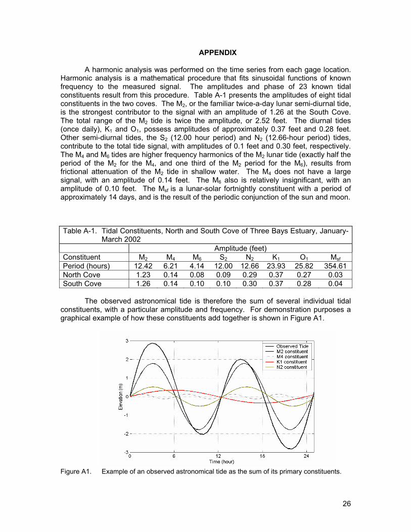
A harmonic analysis was performed on the time series from each gage location. Harmonic analysis is a mathematical procedure that fits sinusoidal functions of known frequency to the measured signal. The amplitudes and phase of 23 known tidal constituents result from this procedure. Table A-1 presents the amplitudes of eight tidal constituents in the two coves. The M2, or the familiar twice-a-day lunar semi-diurnal tide, is the strongest contributor to the signal with an amplitude of 1.26 at the South Cove. The total range of the M2 tide is twice the amplitude, or 2.52 feet. The diurnal tides (once daily), K1 and O1, possess amplitudes of approximately 0.37 feet and 0.28 feet. Other semi-diurnal tides, the S2 (12.00 hour period) and N2 (12.66-hour period) tides, contribute to the total tide signal, with amplitudes of 0.1 feet and 0.30 feet, respectively. The M4 and M6 tides are higher frequency harmonics of the M2 lunar tide (exactly half the period of the M2 for the M4, and one third of the M2 period for the M6), results from frictional attenuation of the M2 tide in shallow water. The M4 does not have a large signal, with an amplitude of 0.14 feet. The M6 also is relatively insignificant, with an amplitude of 0.10 feet. The Msf is a lunar-solar fortnightly constituent with a period of approximately 14 days, and is the result of the periodic conjunction of the sun and moon.

The observed astronomical tide is therefore the sum of several individual tidal

constituents, with a particular amplitude and frequency. For demonstration purposes a graphical example of how these constituents add together is shown in Figure A1.

Figure A1. Example of an observed astronomical tide as the sum of its primary constituents.

Table A-1. Tidal Constituents, North and South Cove of Three Bays Estuary, January-March 2002

Amplitude (feet) Constituent M2 M4 M6 S2 N2 K1 O1 Msf Period (hours) 12.42 6.21 4.14 12.00 12.66 23.93 25.82 354.61 North Cove 1.23 0.14 0.08 0.09 0.29 0.37 0.27 0.03 South Cove 1.26 0.14 0.10 0.10 0.30 0.37 0.28 0.04