feasible descent algorithms for mixed …pages.cs.wisc.edu/~ferris/papers/mp-path.pdffeasible...
TRANSCRIPT
Digital Object Identifier (DOI) 10.1007/s10107990057a
Math. Program. 86: 475–497 (1999) Springer-Verlag 1999
Michael C. Ferris·Christian Kanzow· Todd S. Munson
Feasible descent algorithms for mixed complementarityproblems
Received April 9, 1998 / Revised version received November 23, 1998Published online March 16, 1999
Abstract. In this paper we consider a general algorithmic framework for solving nonlinear mixed comple-mentarity problems. The main features of this framework are: (a) it is well-defined for an arbitrary mixedcomplementarity problem, (b) it generates only feasible iterates, (c) it has a strong global convergence theory,and (d) it is locally fast convergent under standard regularity assumptions. This framework is applied to thePATH solver in order to show viability of the approach. Numerical results for an appropriate modification ofthe PATH solver indicate that this framework leads to substantial computational improvements.
Key words. mixed complementarity problems – global convergence – superlinear convergence – feasibledescent methods
1. Introduction
In the past few years, interest in formulating and solving large scale nonlinear mixedcomplementarity problems (MCP) has become significant and continues to grow. Manytheoretical algorithms have been postulated with numerical successes being reportedfor a variety of them on certain problem classes. Much current research focusses onnonsmooth Newton and smoothing-type methods, which typically have strong theoret-ical foundations and perform well on many test examples. On the other hand, themost widely used algorithms remain those based on successive linearization, whichsolve linear complementarity subproblems using generalizations of the Lemke pivotingalgorithm. These linearization algorithms were proven locally quadratically convergent,and in practice seem to work extremely well. However, they typically require strongtheoretical assumptions in order to guarantee that the subproblems are solvable.
The aim of this paper is twofold. First, we give a theoretical framework for theglobalization of linearization and related algorithms. Second, we apply our theory toone particular linearization method, namely the PATH solver, to demonstrate viability.
M.C. Ferris: University of Wisconsin – Madison, Computer Sciences Department, 1210 West Dayton Street,Madison, WI 53706, USA, e-mail:[email protected] research of this author was partially supported by National Science Foundation Grants CCR-9619765and CDA-9726385.
C. Kanzow: University of Hamburg, Institute of Applied Mathematics, Bundesstrasse 55, D-20146 Hamburg,Germany, e-mail:[email protected] research of this author was supported by the DFG (Deutsche Forschungsgemeinschaft).
T.S. Munson: University of Wisconsin – Madison, Computer Sciences Department, 1210 West Dayton Street,Madison, WI 53706, USA, e-mail:[email protected] research of this author was partially supported by National Science Foundation Grants CCR-9619765and CDA-9726385.

476 Michael C. Ferris et al.
In fact, our modification of the PATH code has better numerical behaviour than allprevious versions of this code.
Merit functions are used extensively in the development of globalization theory andthe implementation of robust algorithms. Broadly speaking, merit functions summarizehow close the current iterate is to a solution of the problem under consideration witha single number. In complementarity problems and nonlinear systems of equations,the merit functions are normally nonnegative, and zero precisely at a solution to theoriginal problem. Each merit function is typically used in a globalization strategy thatinvolves searching between the current iterate and the Newton point (the solution of thelinearization).
The classical example of a merit function in nonlinear equation solving is the squareof the two-norm residual that measures the sum of squares of the errors in satisfyingthe equations. This merit function has one additional property to those listed above:namely, it is everywhere differentiable provided that the equation itself is everywheredifferentiable.
In complementarity, the two classical merit functions are based on the natural re-sidual [25] and the normal map [32]. Both the natural residual and the normal mapprovide reformulations of the complementarity problem as a system of equations; un-fortunately, the systems and corresponding residual merit functions are nonsmooth.Even with this drawback, Ralph [30] showed how to construct an extension of the linesearch procedure for smooth nonlinear equations that enables fast local convergence oflinearization methods under conditions that are exact generalizations of those requiredin smooth systems. This procedure has been implemented and successfully used in thePATH code [10,15].
A key implementational difficulty remains what to do when the linearization sub-problem has no solution. The theory assumes this situation does not happen. In practice,this occurs frequently, particularly if the user of the code does not provide a good initialstarting point. In nonlinear equations, an algorithm can resort to taking a steepest descentdirection for the merit function, guaranteeing progress toward a stationary point of themerit function. Since the merit function used in the PATH solver is not guaranteed tobe differentiable, heuristics need to be implemented to overcome these cases. Whilethese heuristics are quite successful in practice, this situation is nonetheless unsatisfac-tory and prone to failure. This paper is an attempt to provide a theoretically justifiableescape mechanism by using a completely different merit function for the mixed com-plementarity problem in conjunction with the direction generated by a linearizationmethod.
In order to outline the details of the paper, we first recall the definition of the mixedcomplementarity problem. Letl i ∈ IR ∪ {−∞} andui ∈ IR ∪ {∞} be given lower andupper bounds withl i < ui for all i ∈ I , whereI is used throughout this paper to denotethe index set{1, . . . ,n}. Let l andu be then-dimensional vectors with componentsl iandui and assume thatF : [l,u] → IRn is a given function, continuously differentiablein a neighbourhood of the feasible set[l,u]. The mixed complementarity problem

Feasible descent algorithms for mixed complementarity problems 477
consists of finding a vectorx∗ ∈ [l,u] such that exactly one of the following holds:
x∗i = l i and Fi (x∗) > 0,
x∗i = ui and Fi (x∗) < 0,
x∗i ∈ [l i ,ui ] and Fi (x∗) = 0.
The first component of this paper, described in Section 2, is a reformulation ofthe mixed complementarity problem, based on the Fischer-Burmeister function [17].This results in an equivalent nonsmooth system of equations8(x) = 0 where thecorresponding merit function
9(x) := 1
28(x)T8(x) = 1
2‖8(x)‖2
is continuously differentiable. This fact, along with other pertinent properties of9 isthe subject of Section 3.
In the special case of nonlinear complementarity problems, both8 and9 are usedto design unconstrained algorithms for the solution of the problem. Unfortunately, inmany practical situations, the imposed bounds,l andu, on the variables of the mixedcomplementarity problem are important not only for the problem definition but alsobecause the complementarity functionF (or its derivative) may not be defined outsideof these bounds. For example, applications that include fractional powers can causesevere difficulties if the function is evaluated outside the feasible region.
The basic algorithmic framework of this paper does not consider8 directly, butinstead attempts to solve the bound constrained optimization reformulation
min 9(x) s.t. x ∈ [l,u].Section 3 also shows that a constrained stationary point is already a solution of themixed complementarity problem under exactly the same assumptions that are used inorder to prove a similar result for unconstrained stationary points of9.
In Section 4 we present our algorithmic framework and prove that it is well-definedas well as globally and locally fast convergent under very weak assumptions. Thetheory only assumes a pre-existing feasible method that is locally well-defined andsuperlinearly convergent; it is not limited to linearization methods or to the PATH solver.Our algorithmic framework generates iterates that lie within the bounds, resorting toa projected gradient step for the bound constrained problem whenever the pre-existingmethod fails to provide sufficient decrease. We show, however, that our method remainslocally superlinearly convergent.
To demonstrate the practicality of our theory, we give a brief description of an imple-mentation and computational results for a particular instance of our class of algorithmsin Section 5. The implementation is based on a modification of the PATH solver; theresults indicate that the modified PATH solver is more robust than all previous versionsof PATH.
Before proceeding, we give a few words about our notation. IfF is any vector-valued function, we denote its Jacobian at a pointx by F′(x) and let∇F(x) signify thetransposed Jacobian. The gradient of a real-valued functionf will be denoted by∇ fand will always be viewed as a column vector.
478 Michael C. Ferris et al.
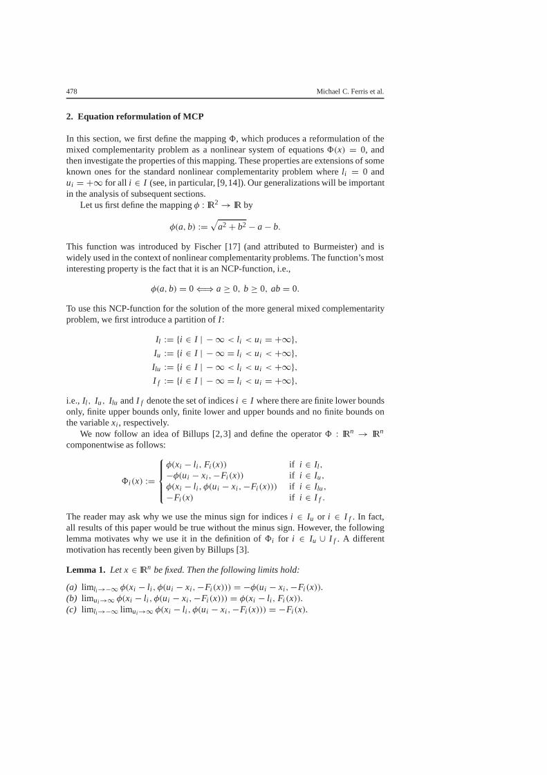
2. Equation reformulation of MCP
In this section, we first define the mapping8, which produces a reformulation of themixed complementarity problem as a nonlinear system of equations8(x) = 0, andthen investigate the properties of this mapping. These properties are extensions of someknown ones for the standard nonlinear complementarity problem wherel i = 0 andui = +∞ for all i ∈ I (see, in particular, [9,14]). Our generalizations will be importantin the analysis of subsequent sections.
Let us first define the mappingφ : IR2→ IR by
φ(a,b) :=√
a2+ b2− a− b.
This function was introduced by Fischer [17] (and attributed to Burmeister) and iswidely used in the context of nonlinear complementarity problems. The function’s mostinteresting property is the fact that it is an NCP-function, i.e.,
φ(a,b) = 0⇐⇒ a ≥ 0, b≥ 0, ab= 0.
To use this NCP-function for the solution of the more general mixed complementarityproblem, we first introduce a partition ofI :
Il := {i ∈ I | −∞ < l i < ui = +∞},Iu := {i ∈ I | −∞ = l i < ui < +∞},Ilu := {i ∈ I | −∞ < l i < ui < +∞},I f := {i ∈ I | −∞ = l i < ui = +∞},
i.e., Il , Iu, Ilu andI f denote the set of indicesi ∈ I where there are finite lower boundsonly, finite upper bounds only, finite lower and upper bounds and no finite bounds onthe variablexi , respectively.
We now follow an idea of Billups [2,3] and define the operator8 : IRn → IRn
componentwise as follows:
8i (x) :=
φ(xi − l i , Fi (x)) if i ∈ Il ,−φ(ui − xi ,−Fi (x)) if i ∈ Iu,
φ(xi − l i , φ(ui − xi ,−Fi (x))) if i ∈ Ilu ,−Fi (x) if i ∈ I f .
The reader may ask why we use the minus sign for indicesi ∈ Iu or i ∈ I f . In fact,all results of this paper would be true without the minus sign. However, the followinglemma motivates why we use it in the definition of8i for i ∈ Iu ∪ I f . A differentmotivation has recently been given by Billups [3].
Lemma 1. Let x ∈ IRn be fixed. Then the following limits hold:
(a) liml i→−∞ φ(xi − l i , φ(ui − xi ,−Fi (x))) = −φ(ui − xi ,−Fi (x)).(b) limui→∞ φ(xi − l i , φ(ui − xi ,−Fi (x))) = φ(xi − l i , Fi (x)).(c) liml i→−∞ limui→∞ φ(xi − l i , φ(ui − xi ,−Fi (x))) = −Fi (x).

Feasible descent algorithms for mixed complementarity problems 479
Proof. Let {ak} ⊆ IR be any sequence converging to∞ and letb ∈ IR be any fixednumber. Then
φ(ak,b) =√(ak)2+ b2− ak − b
=(√(ak)2 + b2− (ak + b)
)(√(ak)2 + b2+ (ak + b)
)√(ak)2 + b2+ (ak + b)
= −2akb√(ak)2+ b2+ (ak + b)
= −2b√1+ (b/ak)2+ 1+ b/ak
→ −b.
From this observation, the three statements follow immediately by simple continuityarguments.
ut
To prove the following characterization of the mixed complementarity problem isstraightforward. The proof is a simple extension of that given in Billups [2, Proposi-tion 3.2.7].
Proposition 1. x∗ ∈ IRn is a solution of the mixed complementarity problem if and onlyif x∗ solves the nonlinear system of equations8(x) = 0.
The function8 is not differentiable everywhere. However, it is locally Lipschitzianand therefore has a nonempty generalized Jacobian in the sense of Clarke [8]. We nextpresent an overestimation of this generalized Jacobian (see Billups [2, Lemma 3.2.10]).
Proposition 2. We have
∂8(x)T ⊆ {Da(x)+ ∇F(x)Db(x)},
where Da(x) ∈ IRn×n and Db(x) ∈ IRn×n are diagonal matrices whose diagonalelements are defined as follows:
(a) If i ∈ Il , then if(xi − l i , Fi (x)) 6= (0,0),
(Da)ii (x) = xi − l i‖(xi − l i , Fi (x))‖ − 1,
(Db)ii (x) = Fi (x)
‖(xi − l i , Fi (x))‖ − 1
but if (xi − l i , Fi (x)) = (0,0),
((Da)ii (x), (Db)ii (x)) ∈ {(ξ − 1, ρ − 1) ∈ IR2| ‖(ξ, ρ)‖ ≤ 1}.
480 Michael C. Ferris et al.
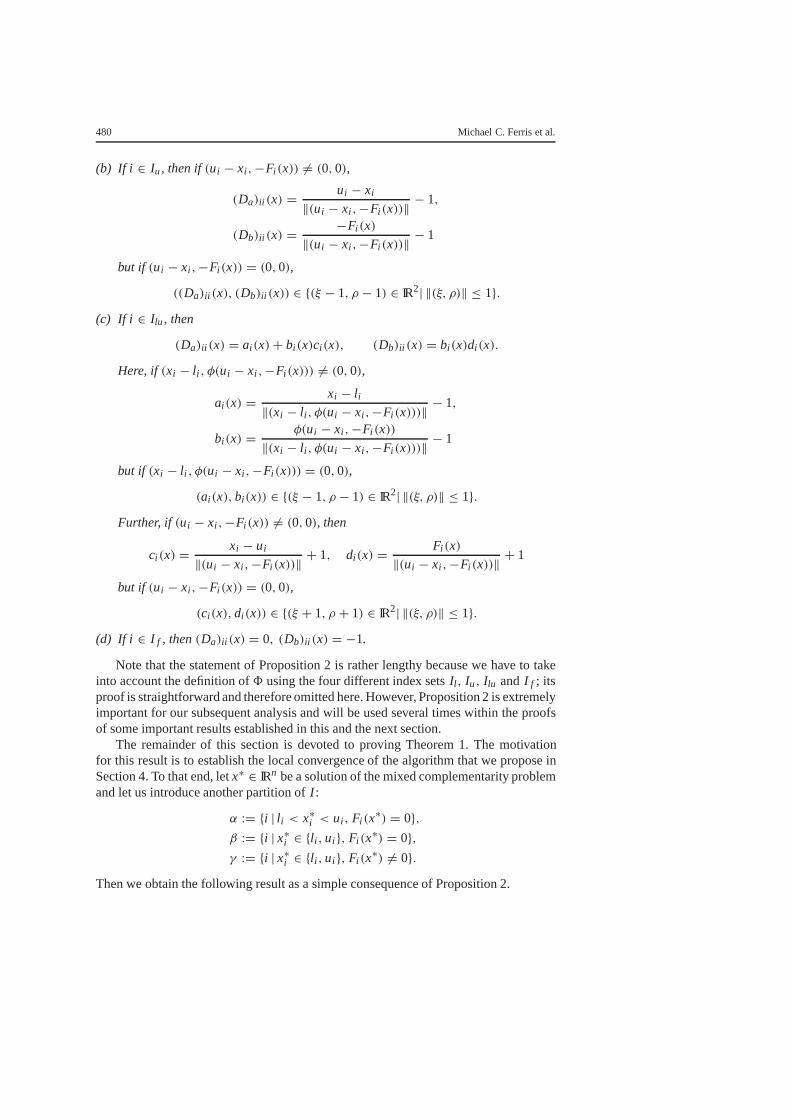
(b) If i ∈ Iu, then if(ui − xi ,−Fi (x)) 6= (0,0),
(Da)ii (x) = ui − xi
‖(ui − xi ,−Fi (x))‖ − 1,
(Db)ii (x) = −Fi (x)
‖(ui − xi ,−Fi (x))‖ − 1
but if (ui − xi ,−Fi (x)) = (0,0),
((Da)ii (x), (Db)ii (x)) ∈ {(ξ − 1, ρ − 1) ∈ IR2| ‖(ξ, ρ)‖ ≤ 1}.(c) If i ∈ Ilu , then
(Da)ii (x) = ai (x)+ bi (x)ci (x), (Db)ii (x) = bi (x)di (x).
Here, if(xi − l i , φ(ui − xi ,−Fi (x))) 6= (0,0),
ai (x) = xi − l i‖(xi − l i , φ(ui − xi ,−Fi (x)))‖ − 1,
bi (x) = φ(ui − xi ,−Fi (x))
‖(xi − l i , φ(ui − xi ,−Fi (x)))‖ − 1
but if (xi − l i , φ(ui − xi ,−Fi (x))) = (0,0),
(ai (x),bi (x)) ∈ {(ξ − 1, ρ − 1) ∈ IR2| ‖(ξ, ρ)‖ ≤ 1}.Further, if (ui − xi ,−Fi (x)) 6= (0,0), then
ci (x) = xi − ui
‖(ui − xi ,−Fi (x))‖ + 1, di (x) = Fi (x)
‖(ui − xi ,−Fi (x))‖ + 1
but if (ui − xi ,−Fi (x)) = (0,0),
(ci (x),di (x)) ∈ {(ξ + 1, ρ + 1) ∈ IR2| ‖(ξ, ρ)‖ ≤ 1}.(d) If i ∈ I f , then(Da)ii (x) = 0, (Db)ii (x) = −1.
Note that the statement of Proposition 2 is rather lengthy because we have to takeinto account the definition of8 using the four different index setsIl , Iu, Ilu and I f ; itsproof is straightforward and therefore omitted here. However, Proposition 2 is extremelyimportant for our subsequent analysis and will be used several times within the proofsof some important results established in this and the next section.
The remainder of this section is devoted to proving Theorem 1. The motivationfor this result is to establish the local convergence of the algorithm that we propose inSection 4. To that end, letx∗ ∈ IRn be a solution of the mixed complementarity problemand let us introduce another partition ofI :
α := {i | l i < x∗i < ui , Fi (x∗) = 0},
β := {i | x∗i ∈ {l i ,ui }, Fi (x∗) = 0},
γ := {i | x∗i ∈ {l i ,ui }, Fi (x∗) 6= 0}.
Then we obtain the following result as a simple consequence of Proposition 2.
Feasible descent algorithms for mixed complementarity problems 481
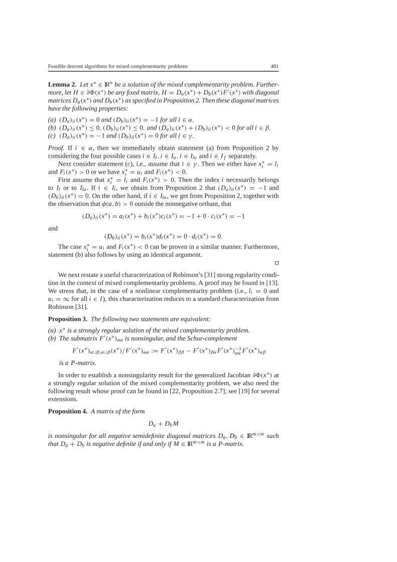
Lemma 2. Let x∗ ∈ IRn be a solution of the mixed complementarity problem. Further-more, letH ∈ ∂8(x∗) be any fixed matrix,H = Da(x∗)+ Db(x∗)F′(x∗) with diagonalmatricesDa(x∗) andDb(x∗) as specified in Proposition 2. Then these diagonal matriceshave the following properties:
(a) (Da)ii (x∗) = 0 and(Db)ii (x∗) = −1 for all i ∈ α.(b) (Da)ii (x∗) ≤ 0, (Db)ii (x∗) ≤ 0, and(Da)ii (x∗)+ (Db)ii (x∗) < 0 for all i ∈ β.(c) (Da)ii (x∗) = −1 and(Db)ii (x∗) = 0 for all i ∈ γ .
Proof. If i ∈ α, then we immediately obtain statement (a) from Proposition 2 byconsidering the four possible casesi ∈ Il , i ∈ Iu, i ∈ Ilu andi ∈ I f separately.
Next consider statement (c), i.e., assume thati ∈ γ . Then we either havex∗i = l iandFi (x∗) > 0 or we havex∗i = ui andFi (x∗) < 0.
First assume thatx∗i = l i and Fi (x∗) > 0. Then the indexi necessarily belongsto Il or to Ilu . If i ∈ Il , we obtain from Proposition 2 that(Da)ii (x∗) = −1 and(Db)ii (x∗) = 0. On the other hand, ifi ∈ Ilu , we get from Proposition 2, together withthe observation thatφ(a,b) > 0 outside the nonnegative orthant, that
(Da)ii (x∗) = ai (x
∗)+ bi (x∗)ci (x
∗) = −1+ 0 · ci (x∗) = −1
and(Db)ii (x
∗) = bi (x∗)di (x
∗) = 0 · di (x∗) = 0.
The casex∗i = ui andFi (x∗) < 0 can be proven in a similar manner. Furthermore,statement (b) also follows by using an identical argument.
utWe next restate a useful characterization of Robinson’s [31] strong regularity condi-
tion in the context of mixed complementarity problems. A proof may be found in [13].We stress that, in the case of a nonlinear complementarity problem (i.e.,l i = 0 andui = ∞ for all i ∈ I ), this characterization reduces to a standard characterization fromRobinson [31].
Proposition 3. The following two statements are equivalent:
(a) x∗ is a strongly regular solution of the mixed complementarity problem.(b) The submatrixF′(x∗)αα is nonsingular, and the Schur-complement
F′(x∗)α∪β,α∪β(x∗)/F′(x∗)αα := F′(x∗)ββ − F′(x∗)βαF′(x∗)−1αα F′(x∗)αβ
is a P-matrix.
In order to establish a nonsingularity result for the generalized Jacobian∂8(x∗) ata strongly regular solution of the mixed complementarity problem, we also need thefollowing result whose proof can be found in [22, Proposition 2.7]; see [19] for severalextensions.
Proposition 4. A matrix of the form
Da + DbM
is nonsingular for all negative semidefinite diagonal matricesDa, Db ∈ IRm×m suchthat Da + Db is negative definite if and only ifM ∈ IRm×m is a P-matrix.

482 Michael C. Ferris et al.
Based on the previous results, we are able to prove the main result of this section.
Theorem 1. If x∗ is a strongly regular solution of the mixed complementarity problem,then all elementsH ∈ ∂8(x∗) are nonsingular.
Proof. Let H ∈ ∂8(x∗). By Proposition 2, there exist diagonal matricesDa(x∗),Db(x∗) ∈ IRn×n such that
H = Da(x∗)+ Db(x
∗)F′(x∗). (1)
Hence, if we write
Da(x∗) =
(Da)αα(x∗) 0 00 (Da)ββ(x∗) 00 0 (Da)γγ (x∗)
,
Db(x∗) =
(Db)αα(x∗) 0 00 (Db)ββ(x∗) 00 0 (Db)γγ (x∗)
and
F′(x∗) = F′(x∗)αα F′(x∗)αβ F′(x∗)αγ
F′(x∗)βα F′(x∗)ββ F′(x∗)βγF′(x∗)γα F′(x∗)γβ F′(x∗)γγ
and if we take into account Lemma 2, the homogeneous linear systemHd = 0 can berewritten as
F′(x∗)ααdα + F′(x∗)αβdβ + F′(x∗)αγdγ = 0α, (2)
(Da)ββ(x∗)dβ + (Db)ββ(x
∗)[F′(x∗)βαdα + F′(x∗)ββdβ + F′(x∗)βγdγ
] = 0β, (3)
−dγ = 0γ . (4)
Sincedγ = 0 by (4) andF′(x∗)αα is nonsingular by assumption and Proposition 3, weobtain from (2):
dα = −F′(x∗)−1αα F′(x∗)αβdβ. (5)
Substituting (4) and (5) into (3), we obtain after some rearrangements:[(Da)ββ(x
∗)+ (Db)ββ(x∗)(F′(x∗)α∪β,α∪β/F′(x∗)αα)
]dβ = 0β. (6)
Since the Schur complementF′(x∗)α∪β,α∪β/F′(x∗)αα is a P-matrix by assumptionand Proposition 3 and since, by Lemma 2 (b), the diagonal matrices(Da)ββ(x∗) and(Db)ββ(x∗) are negative semidefinite with a negative definite sum, it follows fromProposition 4 that the coefficient matrix in (6) is nonsingular. Hence we obtaindβ = 0β.This, in turn, impliesdα = 0α by (5). Reference to (4) shows thatd = 0, so thatH isnonsingular.
ut

Feasible descent algorithms for mixed complementarity problems 483
3. Smooth merit function for MCP
We now investigate the properties of the residual merit function
9(x) = 1
28(x)T8(x)
associated with the equation operator8.Despite the fact that8 is nondifferentiable in general, it turns out that the merit
function9 is continuously differentiable everywhere. More precisely, we have thefollowing result.
Proposition 5. The function 9 is continuously differentiable with gradient∇9(x) = HT8(x) for an arbitrary H ∈ ∂8(x).Proof. The proof is essentially the same as that given for Proposition 3.4 by Facchineiand Soares [14] for the special case of a nonlinear complementarity problem.
utWe next provide a stationary point result for the unconstrained reformulation
min 9(x), x ∈ IRn,
of the mixed complementarity problem. To this end, we need the following characteriza-tion of P0-matrices, see [7] as well as [19] for some generalizations (note the differencebetween this result and the related statement in Proposition 4).
Proposition 6. A matrix of the form
Da + DbM
is nonsingular for all negative definite diagonal matricesDa, Db ∈ IRm×m if and onlyif M ∈ IRm×m is a P0-matrix.
Proposition 6 enables us to prove the first major result of this section. In this resultand in the remaining part of this section, we use the short-hand notation∇F(x∗) f f
to denote the submatrix∇F(x∗)I f I f . A similar notation is used for submatrices andsubvectors defined by other index sets.
Theorem 2. Let x∗ ∈ IRn be a stationary point of9. Assume that
(a) the principal submatrix∇F(x∗) f f is nonsingular, and(b) the Schur complement∇F(x∗)/∇F(x∗) f f is a P0-matrix.
Thenx∗ is a solution of the mixed complementarity problem.
Proof. Let x∗ be a stationary point of9. Then, by Proposition 5, we have
HT8(x∗) = ∇9(x∗) = 0 (7)

484 Michael C. Ferris et al.
for an arbitraryH ∈ ∂8(x∗). By Proposition 2, there exist diagonal matricesDa(x∗),Db(x∗) ∈ IRn×n such that
H = Da(x∗)+ Db(x
∗)F′(x∗).
Therefore, (7) becomes[Da(x
∗)+∇F(x∗)Db(x∗)]8(x∗) = 0. (8)
Writing
Da(x∗) =
((Da) f f (x∗) 0
0 (Da) f̄ f̄ (x∗)
),
Db(x∗) =
((Db) f f (x∗) 0
0 (Db) f̄ f̄ (x∗)
),
and
∇F(x∗) =(∇F(x∗) f f ∇F(x∗) f f̄∇F(x∗) f̄ f ∇F(x∗) f̄ f̄
),
whereI f̄ := I \ I f , and taking into account that
(Da)ii (x∗) = 0 ∀i ∈ I f ,
(Db)ii (x∗) = −1 ∀i ∈ I f
by Proposition 2, we can rewrite (8) as
−∇F(x∗) f f8(x∗) f + ∇F(x∗) f f̄ (Db) f̄ f̄ (x
∗)8(x∗) f̄ = 0 f , (9)
(Da) f̄ f̄ (x∗)8(x∗) f̄ −∇F(x∗) f̄ f8(x
∗) f + ∇F(x∗) f̄ f̄ (Db) f̄ f̄ (x∗)8(x∗) f̄ = 0 f̄ . (10)
Due to the assumed nonsingularity of∇F(x∗) f f , we obtain from (9):
8(x∗) f = ∇F(x∗)−1f f ∇F(x∗) f f̄ (Db) f̄ f̄ (x
∗)8(x∗) f̄ . (11)
Substituting this expression into (10) and rearranging terms gives[(Da) f̄ f̄ (x
∗)+ (∇F(x∗)/∇F(x∗) f f )(Db) f̄ f̄ (x∗)]8(x∗) f̄ = 0 f̄ . (12)
Since
(i) the diagonal matrices(Da) f̄ f̄ (x∗) and(Db) f̄ f̄ (x
∗) have nonpositive entries,(ii) a diagonal element of(Da) f̄ f̄ (x
∗) or (Db) f̄ f̄ (x∗) can be zero only if the corres-
ponding component of8(x∗) f̄ is zero, and(iii) the diagonal matrices(Da) f̄ f̄ (x
∗) and(Db) f̄ f̄ (x∗) are always postmultiplied by
8(x∗) f̄ in the system (9), (10),
we can assume without loss of generality that all diagonal entries ofDa(x∗) andDb(x∗)are negative. But then Proposition 6 and the assumption of our theorem show that thecoefficient matrix in (12) is nonsingular. Hence we get8(x∗) f̄ = 0 f̄ from (12). Butthen (11) implies8(x∗) f = 0 f . Hence8(x∗) = 0, i.e.,x∗ is a solution of the mixedcomplementarity problem by Proposition 1.
ut
Feasible descent algorithms for mixed complementarity problems 485
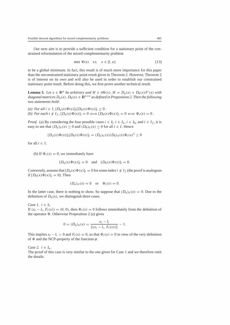
Our next aim is to provide a sufficient condition for a stationary point of the con-strained reformulation of the mixed complementarity problem
min 9(x) s.t. x ∈ [l,u] (13)
to be a global minimum. In fact, this result is of much more importance for this paperthan the unconstrained stationary point result given in Theorem 2. However, Theorem 2is of interest on its own and will also be used in order to establish our constrainedstationary point result. Before doing this, we first prove another technical result.
Lemma 3. Let x ∈ IRn be arbitrary andH ∈ ∂8(x), H = Da(x) + Db(x)F′(x) withdiagonal matricesDa(x), Db(x) ∈ IRn×n as defined in Proposition 2. Then the followingtwo statements hold:
(a) For all i ∈ I , [Da(x)8(x)]i [Db(x)8(x)]i ≥ 0 .(b) For eachi 6∈ I f , [Da(x)8(x)]i = 0⇐⇒ [Db(x)8(x)]i = 0⇐⇒ 8i (x) = 0 .
Proof. (a) By considering the four possible casesi ∈ Il , i ∈ Iu, i ∈ Ilu andi ∈ I f , it iseasy to see that(Da)ii (x) ≤ 0 and(Db)ii (x) ≤ 0 for all i ∈ I . Hence
[Da(x)8(x)]i [Db(x)8(x)]i = (Da)ii (x)(Db)ii (x)8i (x)2 ≥ 0
for all i ∈ I .
(b) If 8i (x) = 0, we immediately have
[Da(x)8(x)]i = 0 and [Db(x)8(x)]i = 0.
Conversely, assume that[Da(x)8(x)]i = 0 for some indexi 6∈ I f (the proof is analogousif [Db(x)8(x)]i = 0). Then
(Da)ii (x) = 0 or 8i (x) = 0.
In the latter case, there is nothing to show. So suppose that(Da)ii (x) = 0. Due to thedefinition of Da(x), we distinguish three cases.
Case 1.i ∈ Il .If (xi − l i , Fi (x)) = (0,0), then8i (x) = 0 follows immediately from the definition ofthe operator8. Otherwise Proposition 2 (a) gives
0= (Da)ii (x) = xi − l i‖(xi − l i , Fi (x))‖ − 1.
This impliesxi − l i > 0 andFi (x) = 0, so that8i (x) = 0 in view of the very definitionof 8 and the NCP-property of the functionφ.
Case 2.i ∈ Iu.The proof of this case is very similar to the one given for Case 1 and we therefore omitthe details.
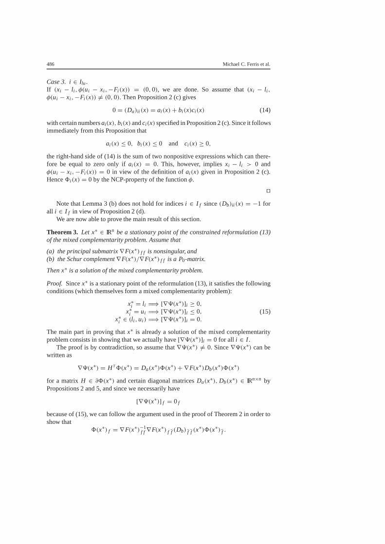
486 Michael C. Ferris et al.
Case 3.i ∈ Ilu .If (xi − l i , φ(ui − xi ,−Fi (x)) = (0,0), we are done. So assume that(xi − l i ,φ(ui − xi ,−Fi (x)) 6= (0,0). Then Proposition 2 (c) gives
0= (Da)ii (x) = ai (x)+ bi (x)ci (x) (14)
with certain numbersai(x),bi (x) andci (x) specified in Proposition 2 (c). Since it followsimmediately from this Proposition that
ai (x) ≤ 0, bi (x) ≤ 0 and ci (x) ≥ 0,
the right-hand side of (14) is the sum of two nonpositive expressions which can there-fore be equal to zero only ifai (x) = 0. This, however, impliesxi − l i > 0 andφ(ui − xi ,−Fi (x)) = 0 in view of the definition ofai (x) given in Proposition 2 (c).Hence8i (x) = 0 by the NCP-property of the functionφ.
utNote that Lemma 3 (b) does not hold for indicesi ∈ I f since(Db)ii (x) = −1 for
all i ∈ I f in view of Proposition 2 (d).We are now able to prove the main result of this section.
Theorem 3. Let x∗ ∈ IRn be a stationary point of the constrained reformulation (13)of the mixed complementarity problem. Assume that
(a) the principal submatrix∇F(x∗) f f is nonsingular, and(b) the Schur complement∇F(x∗)/∇F(x∗) f f is a P0-matrix.
Thenx∗ is a solution of the mixed complementarity problem.
Proof. Sincex∗ is a stationary point of the reformulation (13), it satisfies the followingconditions (which themselves form a mixed complementarity problem):
x∗i = l i H⇒ [∇9(x∗)]i ≥ 0,x∗i = ui H⇒ [∇9(x∗)]i ≤ 0,
x∗i ∈ (l i ,ui ) H⇒ [∇9(x∗)]i = 0.(15)
The main part in proving thatx∗ is already a solution of the mixed complementarityproblem consists in showing that we actually have[∇9(x∗)]i = 0 for all i ∈ I .
The proof is by contradiction, so assume that∇9(x∗) 6= 0. Since∇9(x∗) can bewritten as
∇9(x∗) = HT8(x∗) = Da(x∗)8(x∗)+ ∇F(x∗)Db(x
∗)8(x∗)
for a matrix H ∈ ∂8(x∗) and certain diagonal matricesDa(x∗), Db(x∗) ∈ IRn×n byPropositions 2 and 5, and since we necessarily have
[∇9(x∗)] f = 0 f
because of (15), we can follow the argument used in the proof of Theorem 2 in order toshow that
8(x∗) f = ∇F(x∗)−1f f ∇F(x∗) f f̄ (Db) f̄ f̄ (x
∗)8(x∗) f̄ .
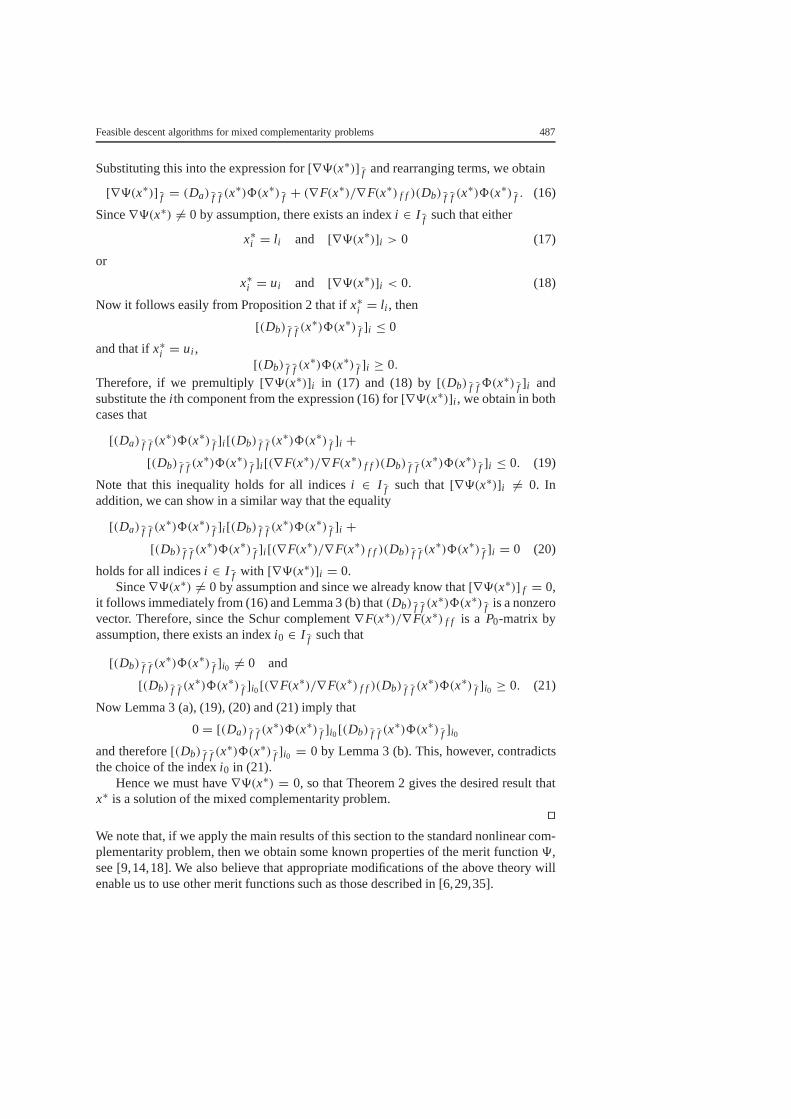
Feasible descent algorithms for mixed complementarity problems 487
Substituting this into the expression for[∇9(x∗)] f̄ and rearranging terms, we obtain
[∇9(x∗)] f̄ = (Da) f̄ f̄ (x∗)8(x∗) f̄ + (∇F(x∗)/∇F(x∗) f f )(Db) f̄ f̄ (x
∗)8(x∗) f̄ . (16)
Since∇9(x∗) 6= 0 by assumption, there exists an indexi ∈ I f̄ such that either
x∗i = l i and [∇9(x∗)]i > 0 (17)
or
x∗i = ui and [∇9(x∗)]i < 0. (18)
Now it follows easily from Proposition 2 that ifx∗i = l i , then
[(Db) f̄ f̄ (x∗)8(x∗) f̄ ]i ≤ 0
and that ifx∗i = ui ,[(Db) f̄ f̄ (x
∗)8(x∗) f̄ ]i ≥ 0.Therefore, if we premultiply[∇9(x∗)]i in (17) and (18) by[(Db) f̄ f̄8(x
∗) f̄ ]i andsubstitute thei th component from the expression (16) for[∇9(x∗)]i , we obtain in bothcases that
[(Da) f̄ f̄ (x∗)8(x∗) f̄ ]i [(Db) f̄ f̄ (x
∗)8(x∗) f̄ ]i +[(Db) f̄ f̄ (x
∗)8(x∗) f̄ ]i [(∇F(x∗)/∇F(x∗) f f )(Db) f̄ f̄ (x∗)8(x∗) f̄ ]i ≤ 0. (19)
Note that this inequality holds for all indicesi ∈ I f̄ such that[∇9(x∗)]i 6= 0. Inaddition, we can show in a similar way that the equality
[(Da) f̄ f̄ (x∗)8(x∗) f̄ ]i [(Db) f̄ f̄ (x
∗)8(x∗) f̄ ]i +[(Db) f̄ f̄ (x
∗)8(x∗) f̄ ]i [(∇F(x∗)/∇F(x∗) f f )(Db) f̄ f̄ (x∗)8(x∗) f̄ ]i = 0 (20)
holds for all indicesi ∈ I f̄ with [∇9(x∗)]i = 0.Since∇9(x∗) 6= 0 by assumption and since we already know that[∇9(x∗)] f = 0,
it follows immediately from (16) and Lemma 3 (b) that(Db) f̄ f̄ (x∗)8(x∗) f̄ is a nonzero
vector. Therefore, since the Schur complement∇F(x∗)/∇F(x∗) f f is a P0-matrix byassumption, there exists an indexi0 ∈ I f̄ such that
[(Db) f̄ f̄ (x∗)8(x∗) f̄ ]i0 6= 0 and
[(Db) f̄ f̄ (x∗)8(x∗) f̄ ]i0[(∇F(x∗)/∇F(x∗) f f )(Db) f̄ f̄ (x
∗)8(x∗) f̄ ]i0 ≥ 0. (21)
Now Lemma 3 (a), (19), (20) and (21) imply that
0= [(Da) f̄ f̄ (x∗)8(x∗) f̄ ]i0[(Db) f̄ f̄ (x
∗)8(x∗) f̄ ]i0and therefore[(Db) f̄ f̄ (x
∗)8(x∗) f̄ ]i0 = 0 by Lemma 3 (b). This, however, contradictsthe choice of the indexi0 in (21).
Hence we must have∇9(x∗) = 0, so that Theorem 2 gives the desired result thatx∗ is a solution of the mixed complementarity problem.
utWe note that, if we apply the main results of this section to the standard nonlinear com-plementarity problem, then we obtain some known properties of the merit function9,see [9,14,18]. We also believe that appropriate modifications of the above theory willenable us to use other merit functions such as those described in [6,29,35].
488 Michael C. Ferris et al.
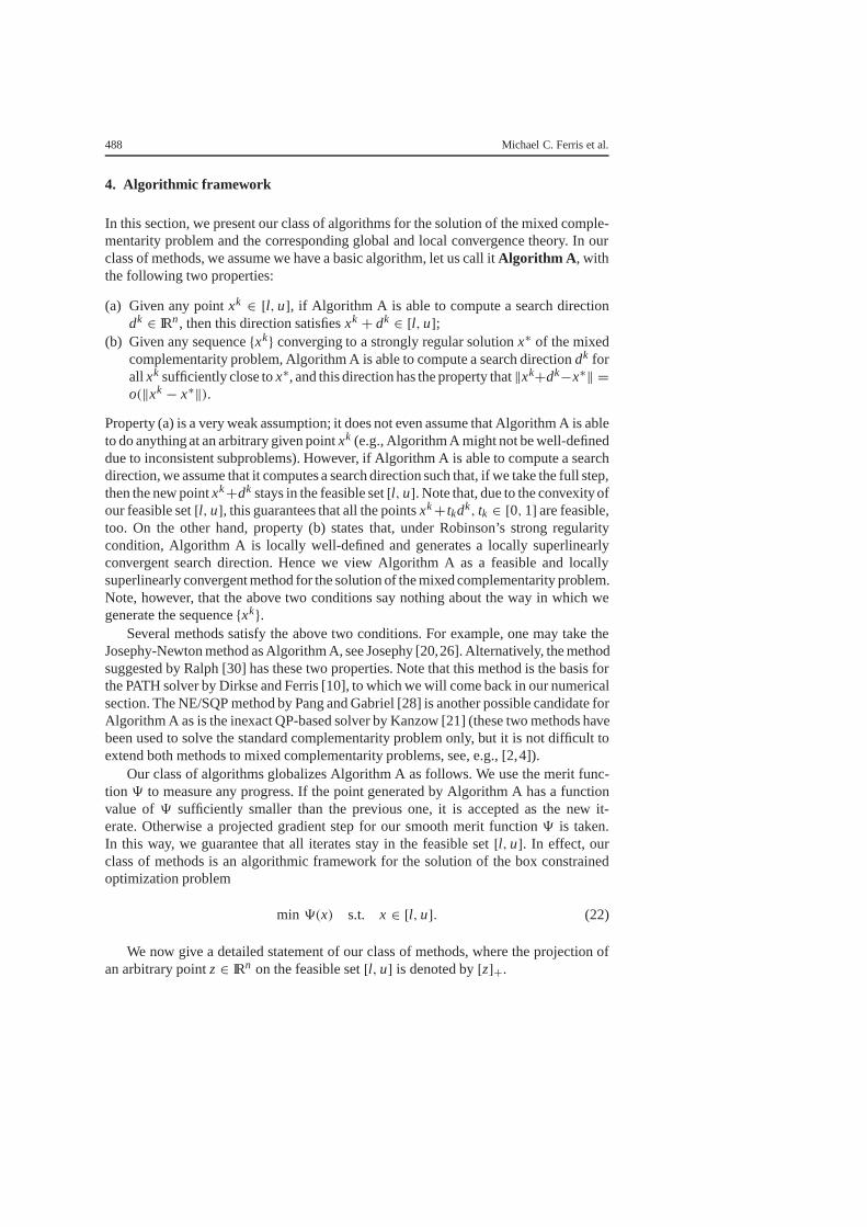
4. Algorithmic framework
In this section, we present our class of algorithms for the solution of the mixed comple-mentarity problem and the corresponding global and local convergence theory. In ourclass of methods, we assume we have a basic algorithm, let us call itAlgorithm A , withthe following two properties:
(a) Given any pointxk ∈ [l,u], if Algorithm A is able to compute a search directiondk ∈ IRn, then this direction satisfiesxk + dk ∈ [l,u];
(b) Given any sequence{xk} converging to a strongly regular solutionx∗ of the mixedcomplementarity problem, Algorithm A is able to compute a search directiondk forall xk sufficiently close tox∗, and this direction has the property that‖xk+dk−x∗‖ =o(‖xk − x∗‖).
Property (a) is a very weak assumption; it does not even assume that Algorithm A is ableto do anything at an arbitrary given pointxk (e.g., Algorithm A might not be well-defineddue to inconsistent subproblems). However, if Algorithm A is able to compute a searchdirection, we assume that it computes a search direction such that, if we take the full step,then the new pointxk+dk stays in the feasible set[l,u]. Note that, due to the convexity ofour feasible set[l,u], this guarantees that all the pointsxk+ tkdk, tk ∈ [0,1] are feasible,too. On the other hand, property (b) states that, under Robinson’s strong regularitycondition, Algorithm A is locally well-defined and generates a locally superlinearlyconvergent search direction. Hence we view Algorithm A as a feasible and locallysuperlinearly convergent method for the solution of the mixed complementarity problem.Note, however, that the above two conditions say nothing about the way in which wegenerate the sequence{xk}.
Several methods satisfy the above two conditions. For example, one may take theJosephy-Newton method as Algorithm A, see Josephy [20,26]. Alternatively, the methodsuggested by Ralph [30] has these two properties. Note that this method is the basis forthe PATH solver by Dirkse and Ferris [10], to which we will come back in our numericalsection. The NE/SQP method by Pang and Gabriel [28] is another possible candidate forAlgorithm A as is the inexact QP-based solver by Kanzow [21] (these two methods havebeen used to solve the standard complementarity problem only, but it is not difficult toextend both methods to mixed complementarity problems, see, e.g., [2,4]).
Our class of algorithms globalizes Algorithm A as follows. We use the merit func-tion9 to measure any progress. If the point generated by Algorithm A has a functionvalue of9 sufficiently smaller than the previous one, it is accepted as the new it-erate. Otherwise a projected gradient step for our smooth merit function9 is taken.In this way, we guarantee that all iterates stay in the feasible set[l,u]. In effect, ourclass of methods is an algorithmic framework for the solution of the box constrainedoptimization problem
min 9(x) s.t. x ∈ [l,u]. (22)
We now give a detailed statement of our class of methods, where the projection ofan arbitrary pointz ∈ IRn on the feasible set[l,u] is denoted by[z]+.

Feasible descent algorithms for mixed complementarity problems 489
Algorithm 1 (General Descent Framework).
Step 1. (Initialization)Choosex0 ∈ [l,u], s> 0, β ∈ (0,1), γ ∈ (0,1) and setk := 0.
Step 2. (Termination Criterion)If xk is a stationary point of (22): STOP.
Step 3. (Compute Fast Search Direction)Use Algorithm A to compute a search directiondk. If this is not possible or if the
condition
9(xk + dk) ≤ γ9(xk) (23)
is not satisfied, go to Step 4, else go to Step 3.
Step 4. (Accept Fast Search Direction)Setxk+1 := xk + dk, k← k+ 1, and go to Step 1.
Step 5. (Take Projected Gradient Step)Computetk = max{sβ`| ` = 0,1,2, . . . } such that
9(xk(tk)) ≤ 9(xk)− σ∇9(xk)T(xk − xk(tk)), (24)
wherexk(t) := [xk − t∇9(xk)]+. Setxk+1 := xk(tk), k← k+ 1, and go to Step 1.
Other methods have attempted to use projected gradient steps in conjunction withsteps that give fast local convergence. See for example, Ferris and Ralph [16]. Unfor-tunately, these hybrid algorithms are difficult to implement and numerical testing hastherefore only been carried out on small test examples. A key difference in the approachoutlined here is that the implementation can be achieved as a minor modification of anexisting code.
We now investigate the convergence properties of our class of methods 1. To thisend, we always assume implicitly that Algorithm 1 does not terminate in a finite numberof steps, i.e., none of the iteratesxk is a stationary point of (22).
We begin with the global convergence analysis that consists of two parts. We firstshow that the algorithm is well-defined, and then we prove that any accumulation pointof a sequence{xk} generated by Algorithm 1 is at least a stationary point of the boundconstrained optimization problem
min 9(x) s.t. x ∈ [l,u]. (25)
Recall that Theorem 3 gives a relatively mild condition for a stationary point of (25) tobe a solution of the mixed complementarity problem.
Theorem 4. Algorithm 1 is well-defined for an arbitrary mixed complementarity prob-lem with a continuously differentiable functionF defined on an open set containing therectangle[l,u].
Furthermore, every accumulation point of a sequence{xk} generated by Algorithm 1is a stationary point of (25).
490 Michael C. Ferris et al.
Proof. To prove the algorithm is well-defined, we only have to show that the projectedgradient step can be carried out at each iteration, i.e., that we can always find a finitesteplengthtk > 0 satisfying condition (24). However, since we assume that none of theiteratesxk is a stationary point of (22), this follows, e.g., from Proposition 2.3.3 (a) inBertsekas [1].
For the second part of the theorem, letx∗ be a stationary point of the sequence{xk},and assume that{xk}K is a subsequence converging tox∗. Suppose there are infinitelymany k ∈ K such thatxk+1 is generated by using a projected gradient step for allthesek. Since the iteratesxk belong to the feasible set[l,u] for all k ∈ IN and since thesequence{9(xk)} is monotonically decreasing, it is not difficult to see that the proofof Proposition 2.3.3 (b) in Bertsekas [1] can be adapted in a straightforward manner toestablish thatx∗ is a stationary point of the constrained reformulation (25).
Hence we can assume without loss of generality that all iteratesk ∈ K satisfy thedescent condition (23). Due to the monotone decrease of the sequence{9(xk)}, thisimplies that the entire sequence{9(xk)} converges to 0. In particular, in view of thedefinition of our merit function, we see that the accumulation pointx∗ is a solution of themixed complementarity problem and hence also a stationary point of problem (25).
utWe next want to show that Algorithm 1 is locally Q-superlinearly convergent underRobinson’s [31] strong regularity condition.
The proof is in two parts. We first show that the entire sequence generated byAlgorithm 1 converges to a solutionx∗ if this solution satisfies the strong regularityassumption. The critical tool to establish this result is the following proposition of Moréand Sorensen [27].
Proposition 7. Assume thatx∗ is an isolated accumulation point of a sequence{xk}(not necessarily generated by Algorithm 1) such that{‖xk+1 − xk‖}K → 0 for anysubsequence{xk}K converging tox∗. Then the whole sequence{xk} converges tox∗.
Once convergence is established, we then determine the rate of convergence. Thebasic device used to show Q-superlinear convergence of our class of methods given in 1is to prove that eventually there are no projected gradient steps, so our method inherits thelocal convergence properties of the locally superlinearly convergent Algorithm A usedin Step 2 of Algorithm 1. To simplify the proof, we invoke the following propositionfrom [23] (see also [14] for a similar result).
Proposition 8. Let G : IRn → IRn be locally Lipschitzian,x∗ ∈ IRn with G(x∗) = 0be such that all elements in∂G(x∗) are nonsingular, and assume that there are twosequences{xk} ⊆ IRn and{dk} ⊆ IRn (not necessarily generated by Algorithm 1) with{xk} → x∗ and‖xk + dk − x∗‖ = o(‖xk − x∗‖). Then‖G(xk + dk)‖ = o(‖G(xk)‖).
We are now in the position to state our main local convergenceresult for Algorithm 1.The convergence rate established here depends critically on the main result of Section 2,namely Theorem 1.
Theorem 5. Let {xk} ⊆ IRn be a sequence generated by Algorithm 1. Assume that thissequence has an accumulation pointx∗ which is a strongly regular solution of the mixed

Feasible descent algorithms for mixed complementarity problems 491
complementarity problem. Then the entire sequence{xk} converges to this point, andthe rate of convergence is Q-superlinear.
Proof. To establish convergence, we first note that a strongly regular solution is anisolated solution of the mixed complementarity problem, see [31]. Since Algorithm 1generates a decreasing sequence{9(xk)} andx∗ is a solution of the mixed complemen-tarity problem, the entire sequence{9(xk)} converges to zero. Hence every accumulationpoint of the sequence{xk} must be a solution of the mixed complementarity problem.Therefore, the assumed strong regularity ofx∗ implies thatx∗ is an isolated accumulationpoint of the sequence{xk}.
Now let {xk}K denote any subsequence converging tox∗. Assume first that we takea projected gradient step for allk ∈ K . Then we obtain, using the nonexpansive propertyof the projection operator:
‖xk+1 − xk‖ = ‖xk(tk)− xk‖= ‖[xk − tk∇9(xk)]+ − xk‖= ‖[xk − tk∇9(xk)]+ − [xk]+‖≤ ‖tk∇9(xk)‖≤ s‖∇9(xk)‖→ 0
(26)
sincex∗ solves the mixed complementarity problem so thatx∗ is a global minimizerand hence a stationary point of our merit function9.
On the other hand, if we calculate the search directiondk by using Algorithm A forinfinitely many k ∈ K , our assumptions on Algorithm A and the assumed strongregularity imply that{dk} → 0 on this infinite subsequence, so that the updating rulesfrom Algorithm 1 show that
‖xk+1 − xk‖ = ‖dk‖ → 0 (27)
on this subsequence. Combining (26) and (27), we immediately obtain that
{‖xk+1 − xk‖}K → 0.
Hence the assumptions of Proposition 7 are satisfied, and convergence follows from thatresult.
In order to establish the Q-superlinear rate, we note that the strong regularity of thesolutionx∗ and Theorem 1 show that all elements in∂8(x∗) are nonsingular. Since, inview of our assumptions about the search directionsdk generated by Algorithm A, wehave‖xk+ dk− x∗‖ = o(‖xk− x∗‖) for these search directions, Proposition 8 impliesthat
‖8(xk + dk)‖ = o(‖8(xk)‖)and therefore
9(xk + dk) = o(9(xk)).
This shows that the descent condition
9(xk + dk) = γ9(xk)

492 Michael C. Ferris et al.
is eventually satisfied in Step 2 of Algorithm 1, i.e., for allk ∈ IN sufficiently large,Algorithm 1 does not take any projected gradient steps. Hence Algorithm 1 has the samelocal convergence properties as Algorithm A. Sincexk+1 = xk + dk, this means that{xk} converges Q-superlinearly tox∗.
utObviously, if the basic Algorithm A is locally Q-quadratically convergent, the class
of Algorithms given in 1 is also locally Q-quadratically convergent. Typically, this holdsif we assume in addition that the Jacobian ofF is locally Lipschitzian.
5. Computational results
The computational results in this section were carried out by extending the PATH 3.0solver to allow use of a different merit function and projected gradient steps. Thecoding was done in ANSI-C and enabled these extensions based on setting the optionmerit_function fischer .
The PATH solver is described in detail in [10,15]. The code is extensively used byeconomists for solving general equilibrium problems and is well known to be robustand efficient on the majority of the mixed complementarity problems it encounters. Thealgorithm successively linearizes the normal map [32] associated with the MCP, definedby
F([y]+)+ y− [y]+where[y]+ represents the projection ofy onto [l,u] in the Euclidean norm, therebygenerating a sequence of linear mixed complementarity problems. These subproblemsare solved by generating a path between the current iterate and the solution of the linearsubproblem; the precise details of this generation scheme can be found for examplein [10]. A nonmonotone backtracking search is performed on this path to garner sufficientdecrease in its merit function, the norm of the residual of the normal map. It is known thatthe solutions of the subproblem will eventually provide descent for the merit function andthat local superlinear or quadratic convergence will occur under appropriate conditions.A crash procedure [12] is used to quickly identify an approximation to the active setat the solution; this is based on a projected Newton step for the normal map, but thedirection produced is not known to be a descent direction for the merit function used.
The PATH 3.0 code was modified to incorporate the extensions that are outlined inthis paper. Two implementational points are of interest. Firstly, a backtracking searchwas implemented instead of the simple test given as (23). This search inspected pointsthat form the following arc, parametrized byt ∈ (0,1]:
[xk + t(xN − xk)]+wherexN is the solution of the linearized normal map. Note that, in general, this isnot the line segment joiningxk to xN. A projected gradient step was only taken ifsuitable descent did not occur for some minimum steplength allowed. This line searchwas chosen to be consistent with that used in the projected gradient step given as (24).

Feasible descent algorithms for mixed complementarity problems 493
Secondly, the gradient of the merit function required for (24) was calculated using theformulas detailed in Propositions 5 and 2 and the method described in [2].
In the following two tables, we give the number of successes and failures of ournew code, PATH 4.0, and the PATH 3.0 code from all starting points in the MCPLIBcollection of test problems [11]. Two tables are presented by splitting the problemsinto standard MCP models (Table 1) and models that were generated using the MPSGEpreprocessor [33,34] in GAMS (Table 2). In order to condense the information in Table 1,we have grouped several similar models together whenever this grouping results in noloss of information; for example, problemscolvdual and colvnlp are groupedtogether as examplecolv* in Table 1.
It was noted in [15] that restarting PATH 3.0 from the user provided starting pointafter the algorithm failed to find a solution on the first attempt significantly improvedthe robustness of the code. In the results reported in Table 1, we use exactly the samerestart parameter settings in both codes (see [15]), with the exception that the PATH 4.0
Table 1.Results for regular models
Problem Without Restarts With RestartsPATH 3.0 PATH 4.0 PATH 3.0 PATH 4.0
asean9a,hanson 3(0) 3(0) 3(0) 3(0)badfree,degen,qp 3(0) 3(0) 3(0) 3(0)bert_oc 4(0) 4(0) 4(0) 4(0)bertsekas,gafni 9(0) 9(0) 9(0) 9(0)billups 0(3) 0(3) 0(3) 0(3)bishop 1(0) 1(0) 1(0) 1(0)bratu,obstacle 9(0) 9(0) 9(0) 9(0)choi,nash 5(0) 5(0) 5(0) 5(0)colv* 10(0) 10(0) 10(0) 10(0)cycle,explcp 2(0) 2(0) 2(0) 2(0)duopoly 0(1) 0(1) 1(0) 1(0)ehl_k* 6(6) 8(4) 11(1) 12(0)electric 0(1) 0(1) 1(0) 1(0)force* 2(0) 2(0) 2(0) 2(0)freebert 7(0) 7(0) 7(0) 7(0)games 16(9) 19(6) 23(2) 25(0)hanskoop 10(0) 10(0) 10(0) 10(0)hydroc*,methan08 3(0) 3(0) 3(0) 3(0)jel,jmu 3(0) 3(0) 3(0) 3(0)josephy,kojshin 15(1) 16(0) 16(0) 16(0)lincont 1(0) 1(0) 1(0) 1(0)mathi* 11(2) 13(0) 13(0) 13(0)ne-hard 1(0) 1(0) 1(0) 1(0)opt_cont* 5(0) 5(0) 5(0) 5(0)pgvon* 6(4) 5(5) 6(4) 6(4)pies 1(0) 1(0) 1(0) 1(0)powell* 12(0) 12(0) 12(0) 12(0)scarf* 12(0) 11(1) 12(0) 12(0)shubik 38(10) 39(9) 48(0) 48(0)simple-* 1(1) 1(1) 1(1) 1(1)sppe,tobin 7(0) 7(0) 7(0) 7(0)tinloi 56(8) 61(3) 63(1) 64(0)trafelas 2(0) 2(0) 2(0) 2(0)
Total 261(46) 273(34) 295(12) 299(8)
494 Michael C. Ferris et al.
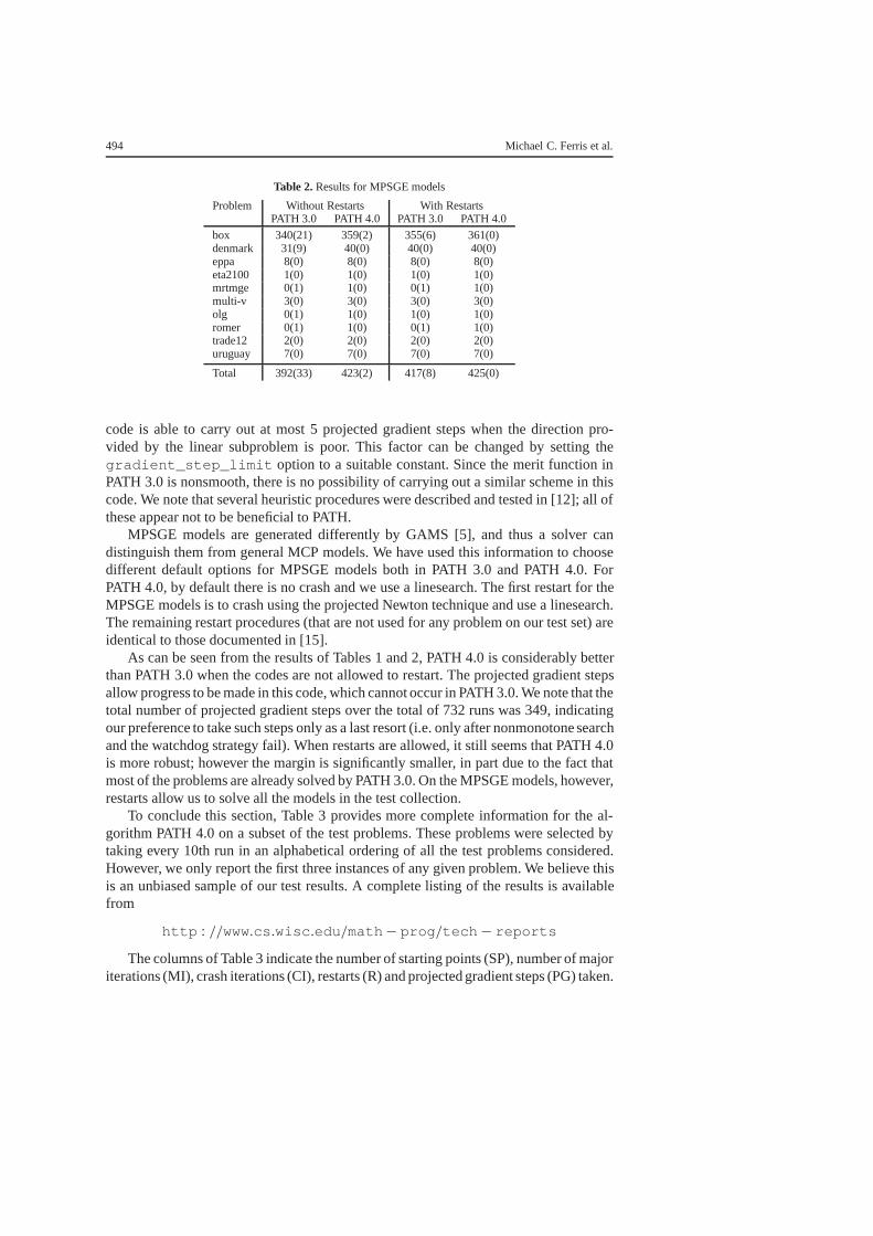
Table 2.Results for MPSGE models
Problem Without Restarts With RestartsPATH 3.0 PATH 4.0 PATH 3.0 PATH 4.0
box 340(21) 359(2) 355(6) 361(0)denmark 31(9) 40(0) 40(0) 40(0)eppa 8(0) 8(0) 8(0) 8(0)eta2100 1(0) 1(0) 1(0) 1(0)mrtmge 0(1) 1(0) 0(1) 1(0)multi-v 3(0) 3(0) 3(0) 3(0)olg 0(1) 1(0) 1(0) 1(0)romer 0(1) 1(0) 0(1) 1(0)trade12 2(0) 2(0) 2(0) 2(0)uruguay 7(0) 7(0) 7(0) 7(0)
Total 392(33) 423(2) 417(8) 425(0)
code is able to carry out at most 5 projected gradient steps when the direction pro-vided by the linear subproblem is poor. This factor can be changed by setting thegradient_step_limit option to a suitable constant. Since the merit function inPATH 3.0 is nonsmooth, there is no possibility of carrying out a similar scheme in thiscode. We note that several heuristic procedures were described and tested in [12]; all ofthese appear not to be beneficial to PATH.
MPSGE models are generated differently by GAMS [5], and thus a solver candistinguish them from general MCP models. We have used this information to choosedifferent default options for MPSGE models both in PATH 3.0 and PATH 4.0. ForPATH 4.0, by default there is no crash and we use a linesearch. The first restart for theMPSGE models is to crash using the projected Newton technique and use a linesearch.The remaining restart procedures (that are not used for any problem on our test set) areidentical to those documented in [15].
As can be seen from the results of Tables 1 and 2, PATH 4.0 is considerably betterthan PATH 3.0 when the codes are not allowed to restart. The projected gradient stepsallow progress to be made in this code, which cannot occur in PATH 3.0. We note that thetotal number of projected gradient steps over the total of 732 runs was 349, indicatingour preference to take such steps only as a last resort (i.e. only after nonmonotone searchand the watchdog strategy fail). When restarts are allowed, it still seems that PATH 4.0is more robust; however the margin is significantly smaller, in part due to the fact thatmost of the problems are already solved by PATH 3.0. On the MPSGE models, however,restarts allow us to solve all the models in the test collection.
To conclude this section, Table 3 provides more complete information for the al-gorithm PATH 4.0 on a subset of the test problems. These problems were selected bytaking every 10th run in an alphabetical ordering of all the test problems considered.However, we only report the first three instances of any given problem. We believe thisis an unbiased sample of our test results. A complete listing of the results is availablefrom
http : //www.cs .wisc .edu/math − prog /tech − reports
The columns of Table 3 indicate the number of starting points (SP), number of majoriterations (MI), crash iterations (CI), restarts (R) and projected gradient steps (PG) taken.

Feasible descent algorithms for mixed complementarity problems 495
Table 3.Selected full results
Problem SP MI CI R PG T
bert_oc 3 0 3 0 0 0.6 (0.4)billups 3 38 2 3 4 * (*)box 9 3 0 0 0 0.0 (0.0)box 19 4 0 0 0 0.0 (0.0)box 29 3 0 0 0 0.0 (0.0)colvnlp 2 3 1 0 0 0.0 (0.0)denmark 4 11 0 0 0 9.9 (25.2)denmark 14 3 0 0 0 2.0 (25.1)denmark 24 11 0 0 0 9.2 (10.3)ehl_k40 3 80 1 1 6 3.4 (*)electric 1 128 1 1 6 2.0 (1.3)explcp 1 1 1 0 0 0.0 (0.0)gafni 1 3 1 0 0 0.0 (0.0)games 8 5 1 0 0 0.1 (0.0)games 18 29 1 0 0 0.2 (0.3)hanskoop 3 6 1 0 0 0.0 (0.0)hydroc06 1 4 1 0 0 0.0 (0.0)josephy 6 5 1 0 0 0.0 (0.0)kojshin 8 1 1 0 0 0.0 (0.0)mathisum 3 7 1 0 0 0.0 (0.0)nash 1 5 1 0 0 0.0 (0.0)obstacle 6 0 7 0 0 1.3 (1.3)pgvon105 2 13 1 0 0 0.2 (0.1)powell 1 6 1 0 0 0.0 (0.0)powell_mcp 5 7 1 0 0 0.0 (0.0)scarfasum 2 3 1 0 0 0.0 (0.0)shubik 4 3 0 0 0 0.0 (0.0)shubik 14 13 1 0 0 0.0 (0.1)shubik 24 41 1 1 5 0.2 (0.1)tinloi 1 1 1 0 0 0.0 (0.0)tinloi 11 1 2 0 0 0.1 (0.0)tinloi 21 1 2 0 0 0.0 (0.0)trafelas 1 7 22 0 0 6.2 (6.3)
The final column of this table reports the time for PATH 4.0 in seconds, with the time forPATH 3.0 added in parentheses. All runs were carried out on a Sun UltraSparc 300 MHzprocessor with 256MB RAM. A “*” indicates failure of the method.
It is hard to draw firm conclusions from Table 3. It indicates that the solution timesof both algorithms are comparable, with some smaller times for PATH 4.0 and somefor PATH 3.0. There are only 4 problems in this subset which use projected gradientsteps and restarts, the vast majority of the problems being solved without invoking thesestrategies.
Overall, the theoretical extensions outlined in this paper result in an improvement inrobustness of PATH 3.0 without any noticeable change in the accuracy or speed of thecode. Further testing on even more challenging problems is required to fully determinethe effects of different merit functions within the PATH code. This will be the subjectof future research.
Acknowledgements.The authors would like to thank Roman Sznajder for pointing out the relation of someof our results with reference [19].
496 Michael C. Ferris et al.
References
1. Bertsekas, D.P. (1995): Nonlinear Programming. Athena Scientific, Belmont, MA2. Billups, S.C. (1995): Algorithms for complementarity problems and generalized equations. Ph.D. Thesis.
Computer Sciences Department, University of Wisconsin, Madison, WI3. Billups, S.C. (1998): A homotopy based algorithm for mixed complementarity problems. Technical
Report. Department of Mathematics, University of Colorado, Denver, CO4. Billups, S.C., Ferris, M.C. (1997): QPCOMP: A quadratic program based solver for mixed complemen-
tarity problems. Math. Program.76, 533–5625. Brooke, A., Kendrick, D., Meeraus, A. (1988): GAMS: A User’s Guide. The Scientific Press, South San
Francisco, CA6. Chen, B., Chen, X., Kanzow, C. (1997): A penalized Fischer-Burmeister NCP-function: Theoretical in-
vestigation and numerical results. Preprint 126, Institute of Applied Mathematics, University of Hamburg,Hamburg (revised May 1998)
7. Chen, B., Harker, P.T. (1993): A noninterior continuation method for quadratic and linear programming.SIAM J. Optim.3, 503–515
8. Clarke, F.H. (1983): Optimization and Nonsmooth Analysis. John Wiley & Sons, New York, NY (reprintedby SIAM, Philadelphia, PA, 1990)
9. De Luca, T., Facchinei, F., Kanzow, C. (1996): A semismooth equation approach to the solution ofnonlinear complementarity problems. Math. Program.75, 407–439
10. Dirkse, S.P., Ferris, M.C. (1995): The PATH solver: A non-monotone stabilization scheme for mixedcomplementarity problems. Optim. Methods Software5, 123–156
11. Dirkse, S.P., Ferris, M.C. (1995): MCPLIB: A collection of nonlinear mixed complementarity problems.Optim. Methods Software5, 319–345
12. Dirkse, S.P., Ferris, M.C. (1997): Crash techniques for large-scale complementarity problems. In: Ferris,M.C., Pang, J.-S., eds., Complementarity and Variational Problems: State of the Art, pp. 40–61. SIAM,Philadelphia, PA
13. Facchinei, F., Fischer, A., Kanzow, C. (1997): A semismooth Newton method for variational inequalities:The case of box constraints. In: Ferris, M.C., Pang, J.-S., eds., Complementarity and VariationalProblems: State of the Art, pp. 76–90. SIAM, Philadelphia
14. Facchinei, F., Soares:, J. (1997): A new merit function for nonlinear complementarity problems anda related algorithm. SIAM J. Optim.7, 225–247
15. Ferris, M.C., Munson, T.S. (1999): Interfaces to PATH 3.0: Design, implementation and usage. Comput.Optim. Appl.12, 207–227
16. Ferris, M.C., Ralph, D. (1995): Projected gradient methods for nonlinear complementarity problems vianormal maps. In: Du, D., Qi, L., Womersley, R., eds., Recent Advances in Nonsmooth Optimization,pp. 57–87. World Scientific Publishers
17. Fischer, A. (1992): A special Newton-type optimization method. Optim.24, 269–28418. Fischer, A. (1998): A new constrained optimization reformulation for complementarity problems. J. Op-
tim. Theory Appl.97, 105–11719. Gowda, M.S., Snajder, R. (1995): Generalizations ofP0- and P-properties; extended vertical and ho-
rizontal LCPs. Lin. Alg. Appl.223/224, 695–71520. Josephy, N.H. (1979): Newton’s method for generalized equations. Technical Summary Report 1965.
Mathematics Research Center, University of Wisconsin, Madison, WI21. Kanzow, C.: An inexact QP-based method for nonlinear complementarity problems. Numer. Math., to
appear22. Kanzow, C., Kleinmichel, H. (1998): A new class of semismooth Newton-type methods for nonlinear
complementarity problems. Comput. Optim. Appl.11, 227–25123. Kanzow, C., Qi, H.-D.: A QP-free constrained Newton-type method for variational inequality problems.
Math. Program., to appear [doi: 10.1007/s10107980007a]24. Liu, J. (1995): Strong stability in variational inequalities. SIAM J. Control Optim.33, 725–74925. Luo, Z.-Q., Tseng, P. (1992): Error bound and convergence analysis of matrix splitting algorithms for the
affine variational inequality problem. SIAM J. Optim.2, 43–5426. Mathiesen, L. (1987): An algorithm based on a sequence of linear complementarity problems applied to
a Walrasian equilibrium model: an example. Math. Program.37, 1–1827. Moré, J.J., Sorensen, D.C. (1983): Computing a trust region step. SIAM J. Scientific Stat. Comput.4,
553–57228. Pang, J.-S., Gabriel, S.A. (1993): NE/SQP: A robust algorithm for the nonlinear complementarity prob-
lem. Math. Program.60, 295–337

Feasible descent algorithms for mixed complementarity problems 497
29. Qi:, L. (1997): Regular pseudo-smooth NCP and BVIP functions and globally and quadratically con-vergent generalized Newton methods for complementarity and variational inequality problems. AppliedMathematics Report AMR 97/14. School of Mathematics, University of New South Wales, Sydney,Australia (revised September 1997)
30. Ralph, D. (1994): Global convergence of Newton’s method for nonsmooth equations via the path search.Math. Oper. Res.19, 352–389
31. Robinson, S.M. (1980): Strongly regular generalized equations. Math. Oper. Res.5, 43–6232. Robinson, S.M. (1992): Normal maps induced by linear transformations. Math. Oper. Res.17, 691–71433. Rutherford, T.F. (1995): Extensions of GAMS for complementarity problems arising in applied economic
analysis. J. Econ. Dyn. Control19, 1299–132434. Rutherford, T.F. (1997): Applied general equilibrium modeling with MPSGE as a GAMS subsystem: An
overview of the modeling framework and syntax. Comput. Econ., to appear35. Sun, D., Womersley, R.S.: A new unconstrained differentiable merit function for box constrained varia-
tional inequality problems and a damped Gauss-Newton method. SIAM J. Optim., to appear