feat 3 - advanced fmri analysis · feat 3 - advanced fmri analysis pipeline overview advanced...
TRANSCRIPT
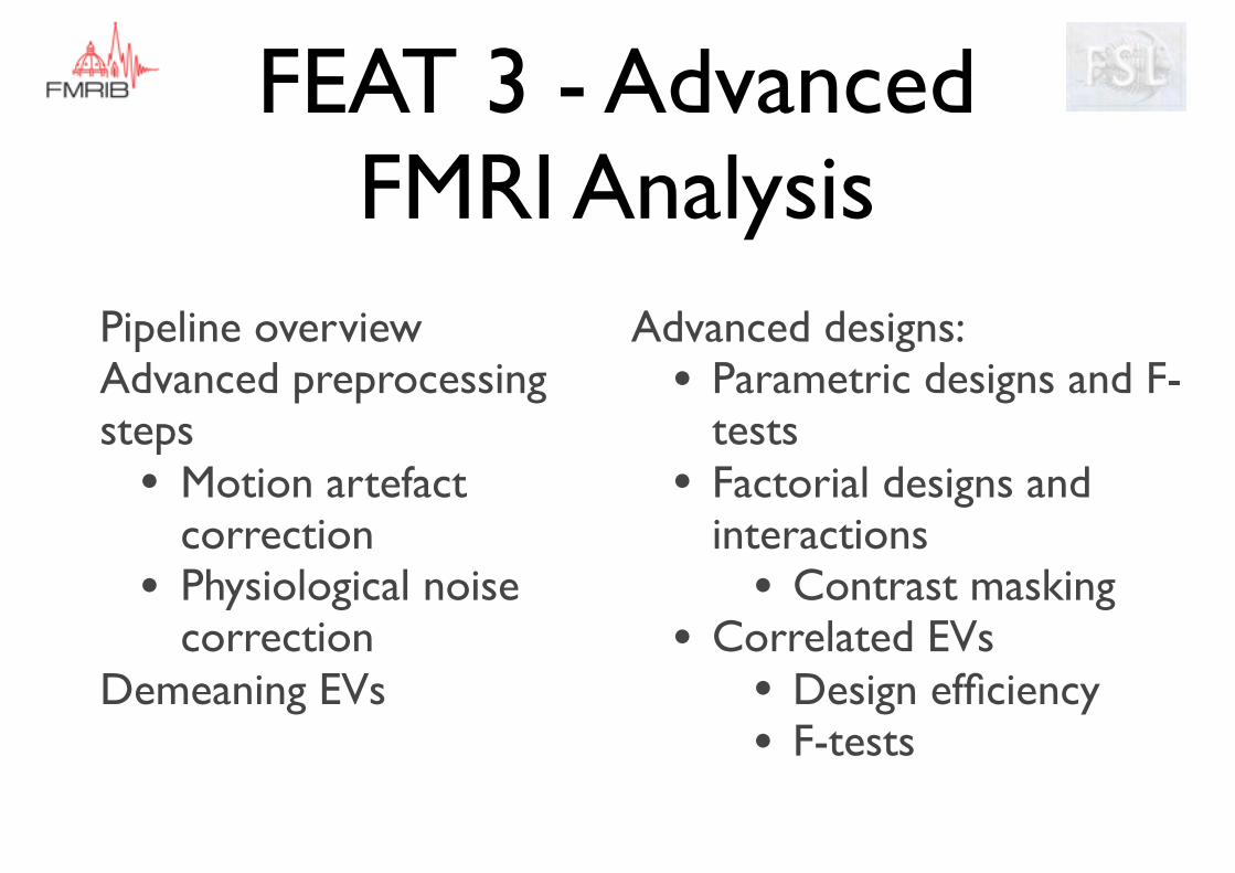
FEAT 3 - Advanced FMRI Analysis
Pipeline overviewAdvanced preprocessing steps
• Motion artefact correction
• Physiological noise correction
Demeaning EVs
Advanced designs:• Parametric designs and F-
tests• Factorial designs and
interactions• Contrast masking
• Correlated EVs• Design efficiency• F-tests

Pipeline overview

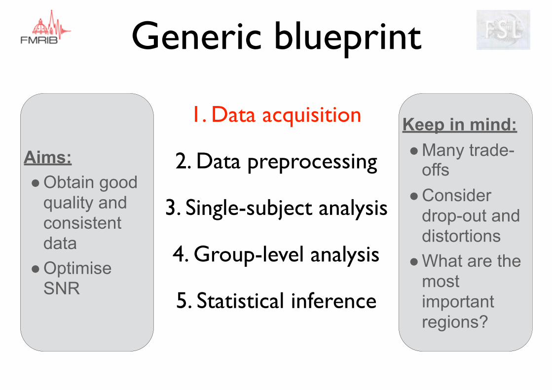
Generic blueprint
1. Data acquisition
2. Data preprocessing
3. Single-subject analysis
4. Group-level analysis
5. Statistical inference
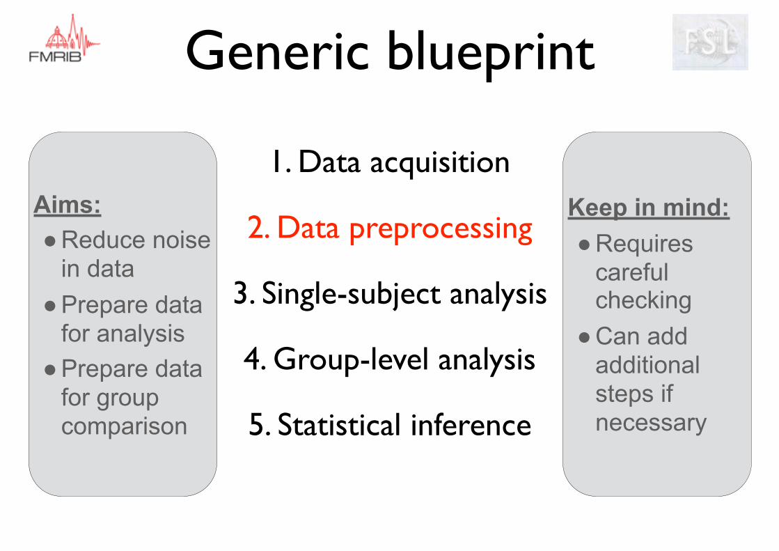
Generic blueprint
1. Data acquisition
2. Data preprocessing
3. Single-subject analysis
4. Group-level analysis
5. Statistical inference
Aims: ●Obtain good
quality and consistent data
●Optimise SNR
Keep in mind: ●Many trade-
offs ●Consider
drop-out and distortions
●What are the most important regions?
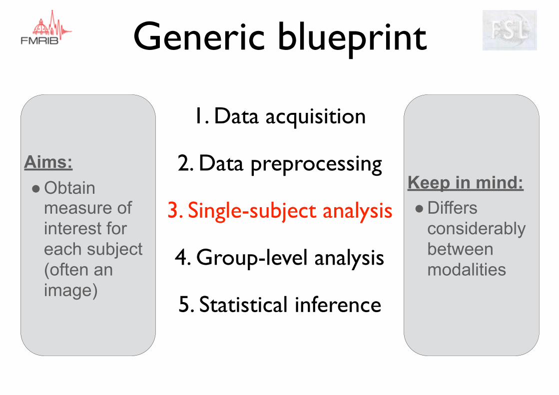
Generic blueprint
1. Data acquisition
2. Data preprocessing
3. Single-subject analysis
4. Group-level analysis
5. Statistical inference
Aims: ●Reduce noise
in data ●Prepare data
for analysis ●Prepare data
for group comparison
Keep in mind: ●Requires
careful checking
●Can add additional steps if necessary
Generic blueprint
1. Data acquisition
2. Data preprocessing
3. Single-subject analysis
4. Group-level analysis
5. Statistical inference
Aims: ●Obtain
measure of interest for each subject (often an image)
Keep in mind: ●Differs
considerably between modalities
Generic blueprint
1. Data acquisition
2. Data preprocessing
3. Single-subject analysis
4. Group-level analysis
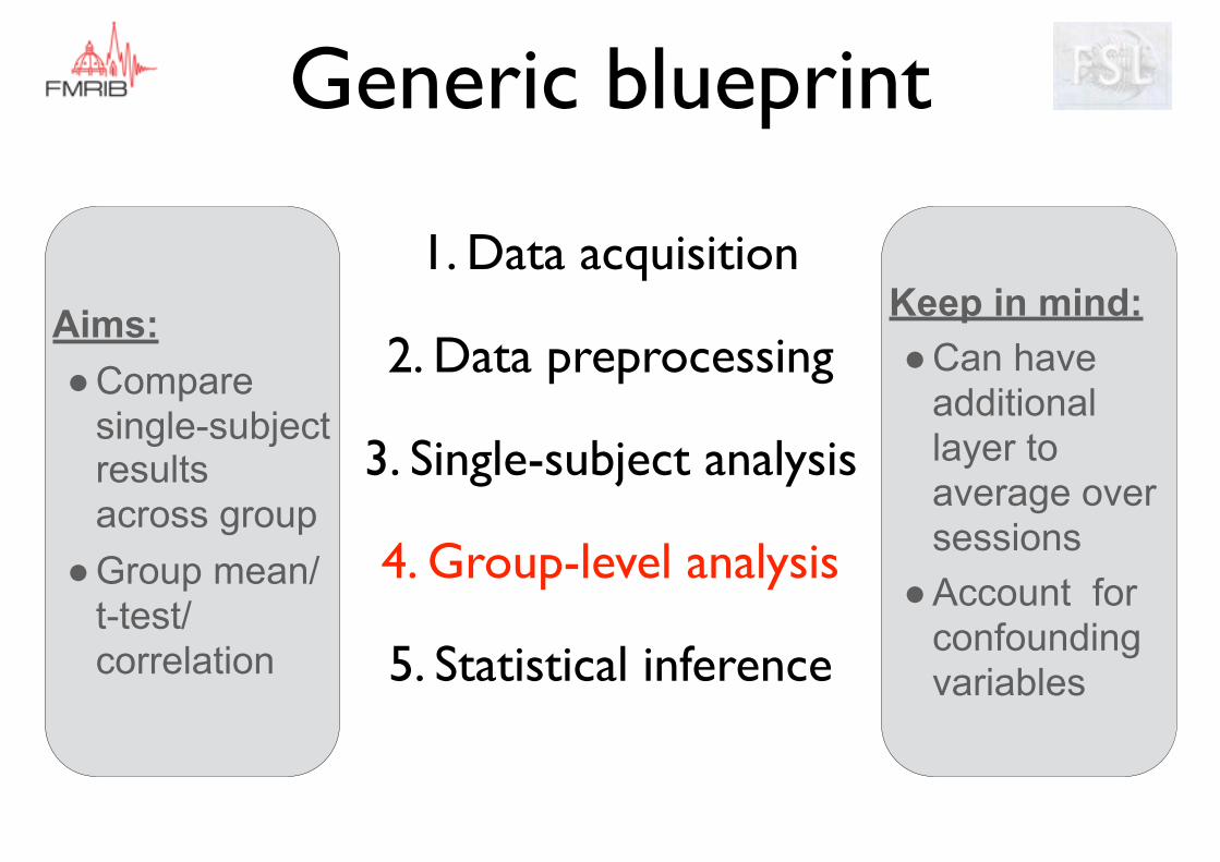
5. Statistical inference
Aims: ●Compare
single-subject results across group
●Group mean/ t-test/ correlation
Keep in mind: ●Can have
additional layer to average over sessions
●Account for confounding variables
Generic blueprint
1. Data acquisition
2. Data preprocessing
3. Single-subject analysis
4. Group-level analysis
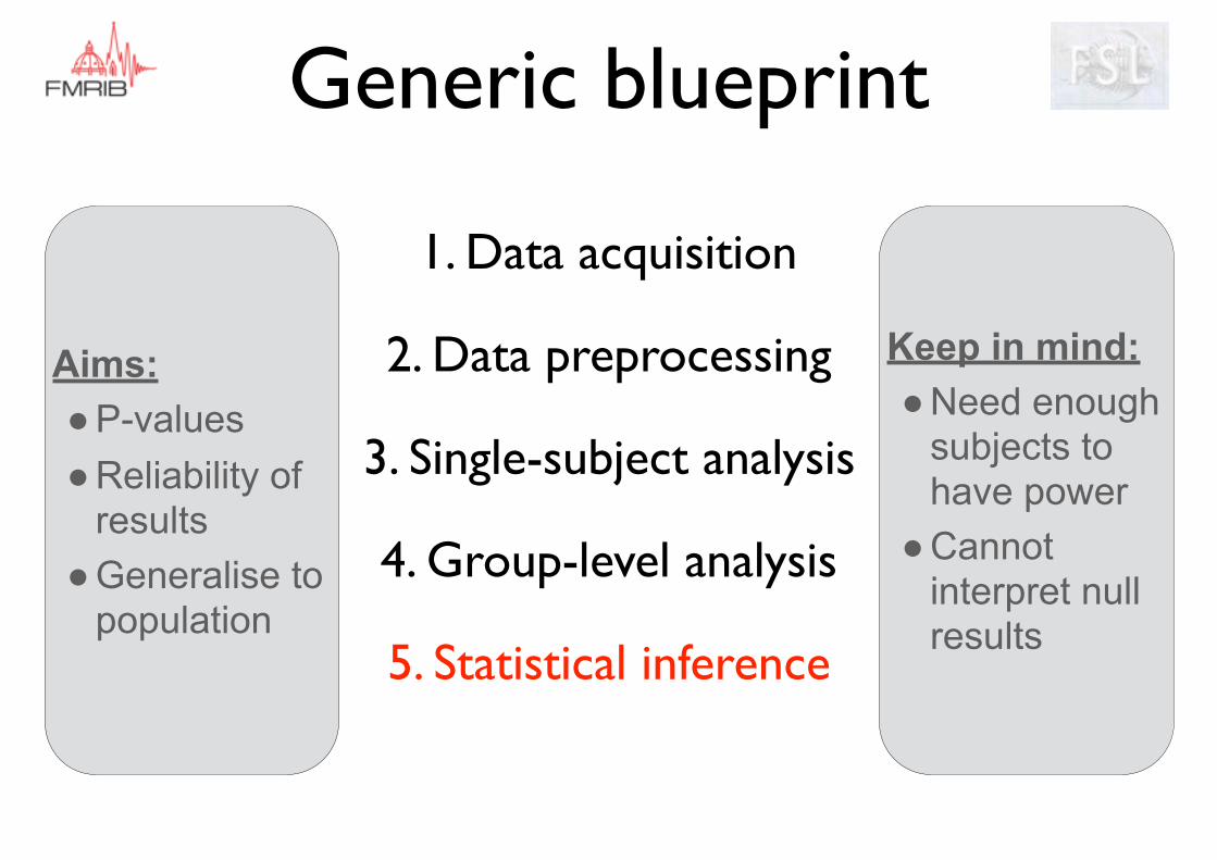
5. Statistical inference
Aims: ●P-values ●Reliability of
results ●Generalise to
population
Keep in mind: ●Need enough
subjects to have power
●Cannot interpret null results
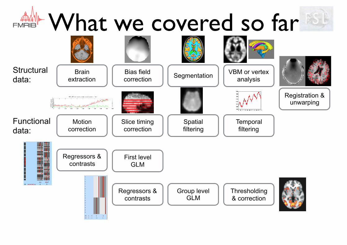
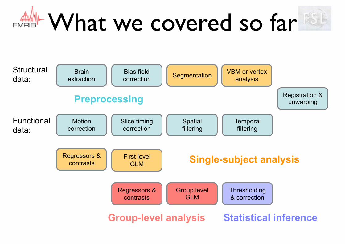
What we covered so far
Brain extraction
Motion correction
Slice timing correction
Spatial filtering
Temporal filtering
Registration & unwarping
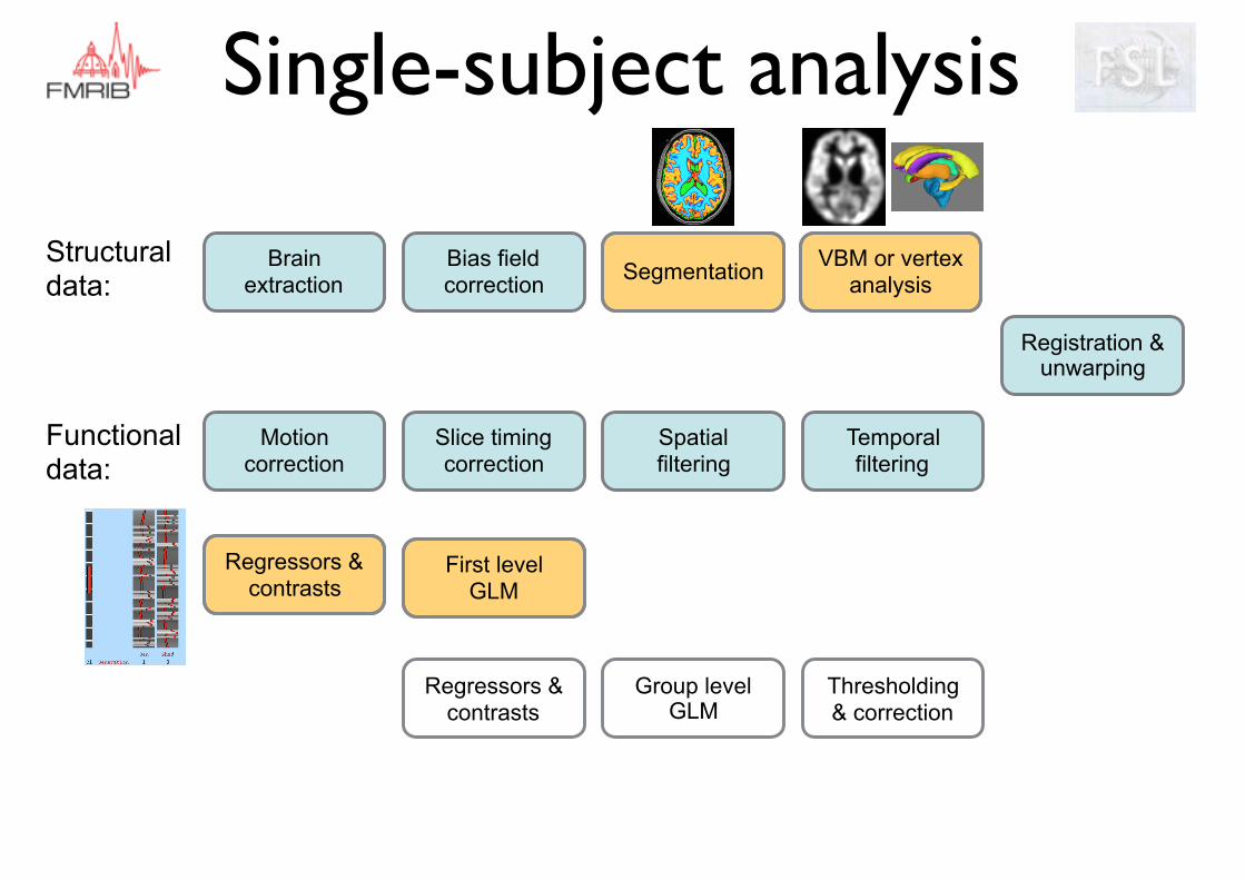
Structural data:
Functional data:
Regressors & contrasts
First level GLM
Group level GLM
Thresholding & correction
Regressors & contrasts
Bias field correction Segmentation VBM or vertex
analysis
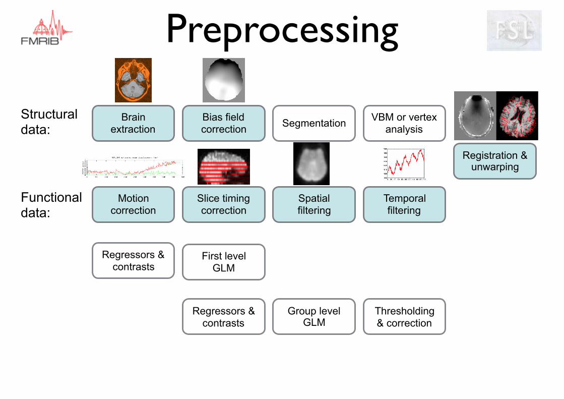
Preprocessing
Motion correction
Slice timing correction
Spatial filtering
Temporal filtering
Registration & unwarping
Structural data:
Functional data:
Regressors & contrasts
First level GLM
Group level GLM
Thresholding & correction
Regressors & contrasts
Bias field correction SegmentationBrain
extractionVBM or vertex
analysis
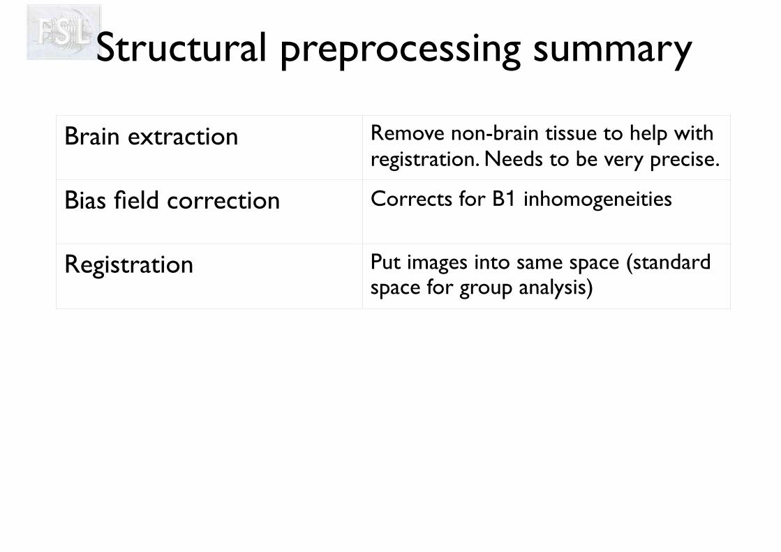
Brain extraction Remove non-brain tissue to help with registration. Needs to be very precise.
Bias field correction Corrects for B1 inhomogeneities
Registration Put images into same space (standard space for group analysis)
Structural preprocessing summary
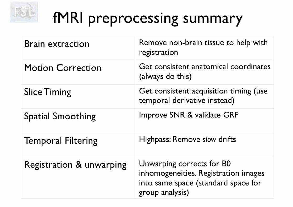
fMRI preprocessing summary
Brain extraction Remove non-brain tissue to help with registration
Motion Correction Get consistent anatomical coordinates (always do this)
Slice Timing Get consistent acquisition timing (use temporal derivative instead)
Spatial Smoothing Improve SNR & validate GRF
Temporal Filtering Highpass: Remove slow drifts
Registration & unwarping Unwarping corrects for B0 inhomogeneities. Registration images into same space (standard space for group analysis)
Motion correction
Slice timing correction
Spatial filtering
Temporal filtering
Registration & unwarping
Structural data:
Functional data:
Regressors & contrasts
First level GLM
Group level GLM
Thresholding & correction
Regressors & contrasts
Bias field correction Segmentation VBM or vertex
analysisBrain
extraction
Single-subject analysis
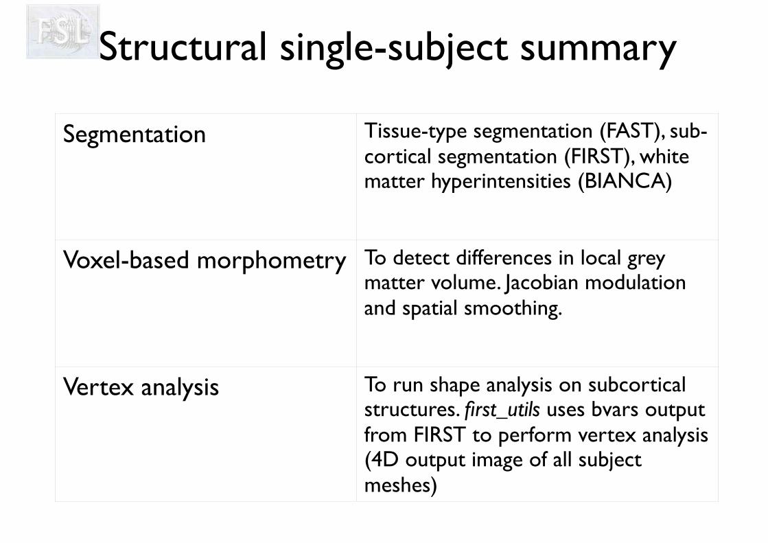
Structural single-subject summary
Segmentation Tissue-type segmentation (FAST), sub-cortical segmentation (FIRST), white matter hyperintensities (BIANCA)
Voxel-based morphometry To detect differences in local grey matter volume. Jacobian modulation and spatial smoothing.
Vertex analysis To run shape analysis on subcortical structures. first_utils uses bvars output from FIRST to perform vertex analysis (4D output image of all subject meshes)
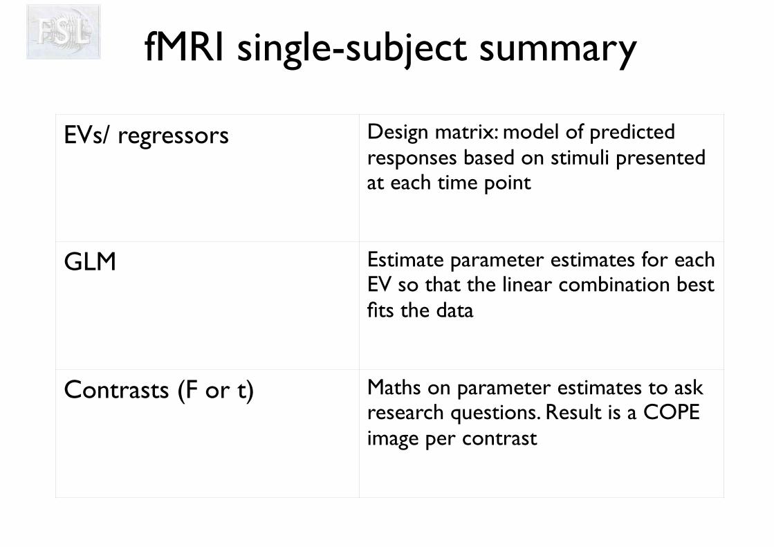
fMRI single-subject summary
EVs/ regressors Design matrix: model of predicted responses based on stimuli presented at each time point
GLM Estimate parameter estimates for each EV so that the linear combination best fits the data
Contrasts (F or t) Maths on parameter estimates to ask research questions. Result is a COPE image per contrast
Motion correction
Slice timing correction
Spatial filtering
Temporal filtering
Registration & unwarping
Structural data:
Functional data:
Regressors & contrasts
First level GLM
Group level GLM
Thresholding & correction
Regressors & contrasts
Bias field correction Segmentation VBM or vertex
analysisBrain
extraction
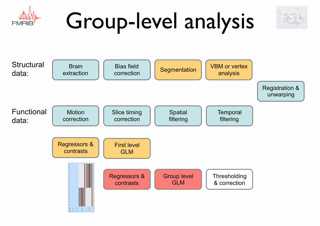
Group-level analysis
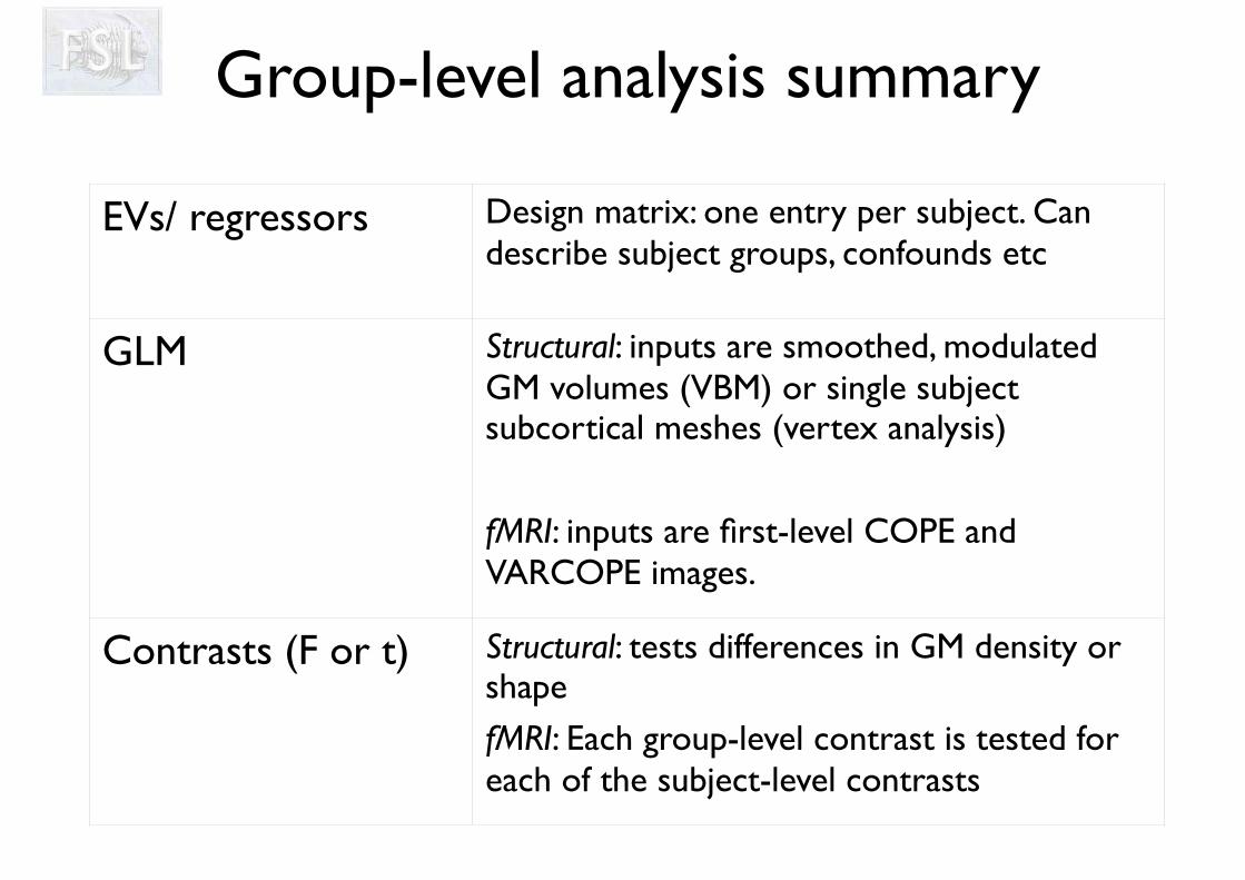
Group-level analysis summary
EVs/ regressors Design matrix: one entry per subject. Can describe subject groups, confounds etc
GLM Structural: inputs are smoothed, modulated GM volumes (VBM) or single subject subcortical meshes (vertex analysis)
fMRI: inputs are first-level COPE and VARCOPE images.
Contrasts (F or t) Structural: tests differences in GM density or shapefMRI: Each group-level contrast is tested for each of the subject-level contrasts
Motion correction
Slice timing correction
Spatial filtering
Temporal filtering
Registration & unwarping
Structural data:
Functional data:
Regressors & contrasts
First level GLM
Group level GLM
Thresholding & correction
Regressors & contrasts
Bias field correction Segmentation VBM or vertex
analysisBrain
extraction
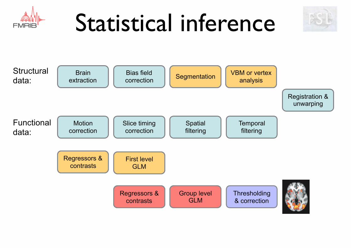
Statistical inference
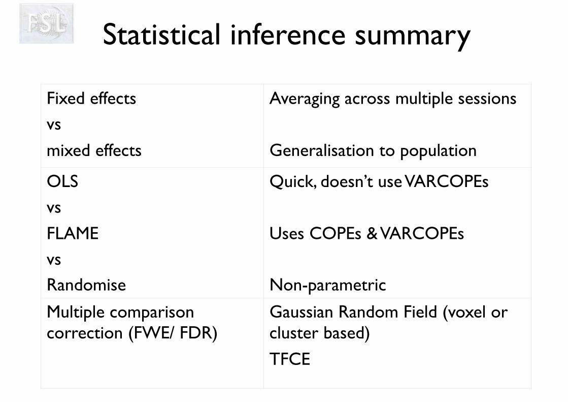
Statistical inference summary
Fixed effects vs
mixed effects
Averaging across multiple sessions
Generalisation to population
OLS vs
FLAMEvsRandomise
Quick, doesn’t use VARCOPEs
Uses COPEs & VARCOPEs
Non-parametric
Multiple comparison correction (FWE/ FDR)
Gaussian Random Field (voxel or cluster based)
TFCE
Motion correction
Slice timing correction
Spatial filtering
Temporal filtering
Registration & unwarping
Structural data:
Functional data:
Regressors & contrasts
First level GLM
Group level GLM
Thresholding & correction
Regressors & contrasts
Bias field correction Segmentation VBM or vertex
analysisBrain
extraction
Preprocessing
Single-subject analysis
Group-level analysis Statistical inference
What we covered so far
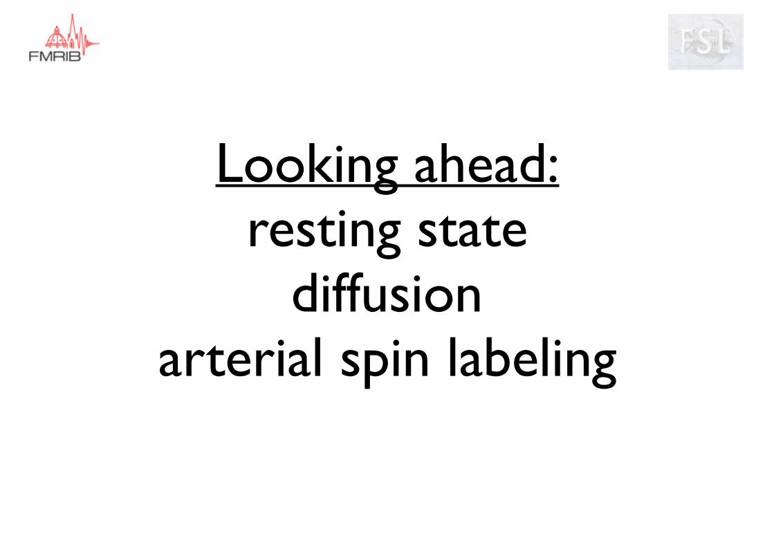
Looking ahead:resting state
diffusionarterial spin labeling
Generic blueprint
1. Data acquisition
2. Data preprocessing
3. Single-subject analysis
4. Group-level analysis
5. Statistical inference
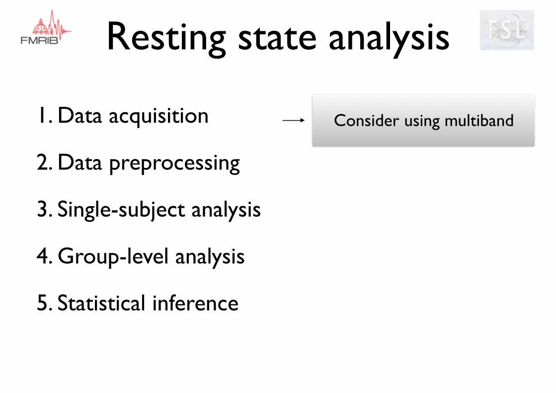
Resting state analysis
1. Data acquisition
2. Data preprocessing
3. Single-subject analysis
4. Group-level analysis
5. Statistical inference
Consider using multiband
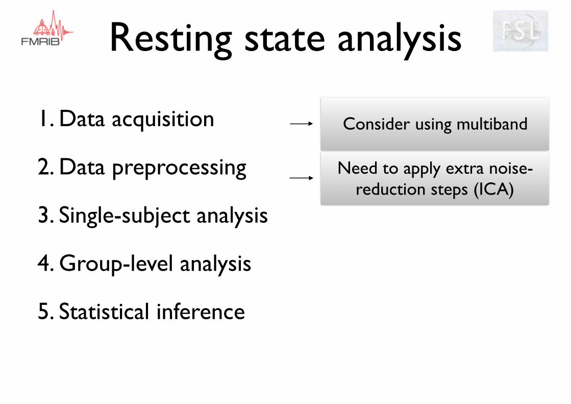
Resting state analysis
1. Data acquisition
2. Data preprocessing
3. Single-subject analysis
4. Group-level analysis
5. Statistical inference
Need to apply extra noise-reduction steps (ICA)
Consider using multiband
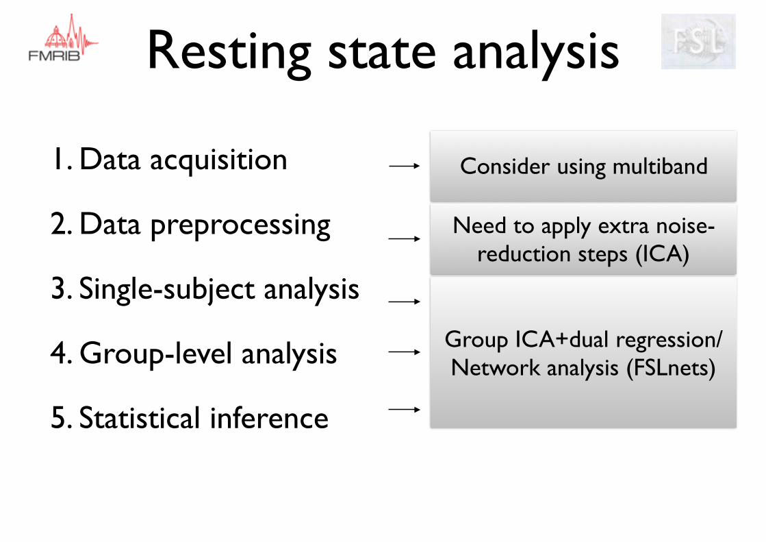
Resting state analysis
1. Data acquisition
2. Data preprocessing
3. Single-subject analysis
4. Group-level analysis
5. Statistical inference
Group ICA+dual regression/Network analysis (FSLnets)
Consider using multiband
Need to apply extra noise-reduction steps (ICA)
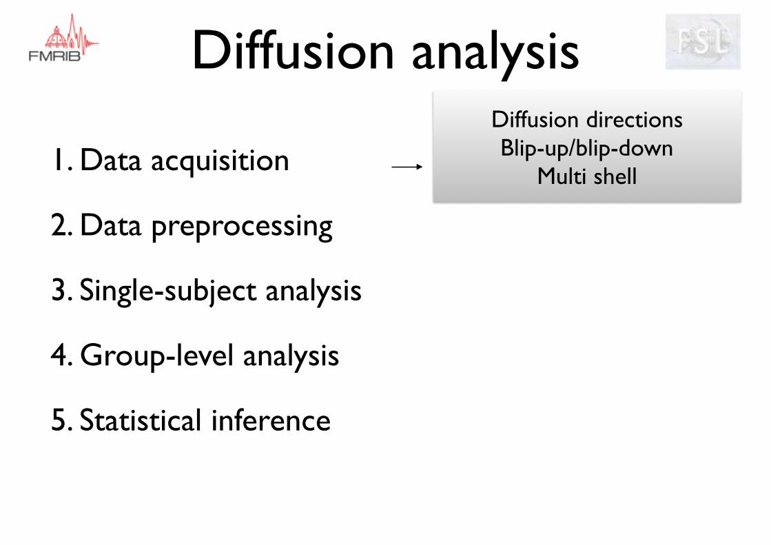
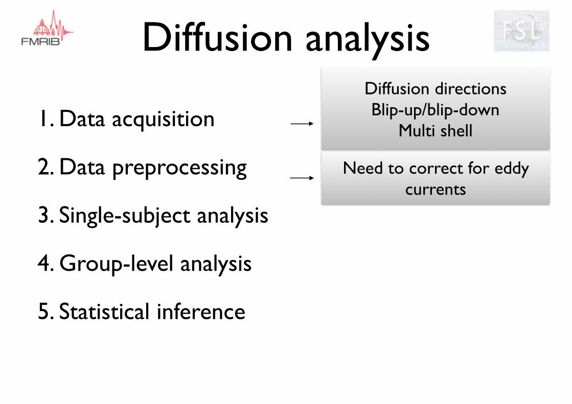
Diffusion analysis
1. Data acquisition
2. Data preprocessing
3. Single-subject analysis
4. Group-level analysis
5. Statistical inference
Diffusion directionsBlip-up/blip-down
Multi shell
Diffusion analysis
1. Data acquisition
2. Data preprocessing
3. Single-subject analysis
4. Group-level analysis
5. Statistical inference
Need to correct for eddy currents
Diffusion directionsBlip-up/blip-down
Multi shell
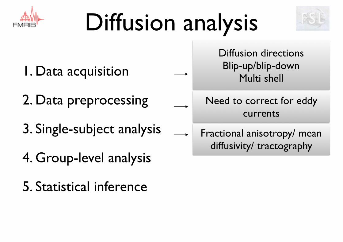
Diffusion analysis
1. Data acquisition
2. Data preprocessing
3. Single-subject analysis
4. Group-level analysis
5. Statistical inference
Need to correct for eddy currents
Fractional anisotropy/ mean diffusivity/ tractography
Diffusion directionsBlip-up/blip-down
Multi shell
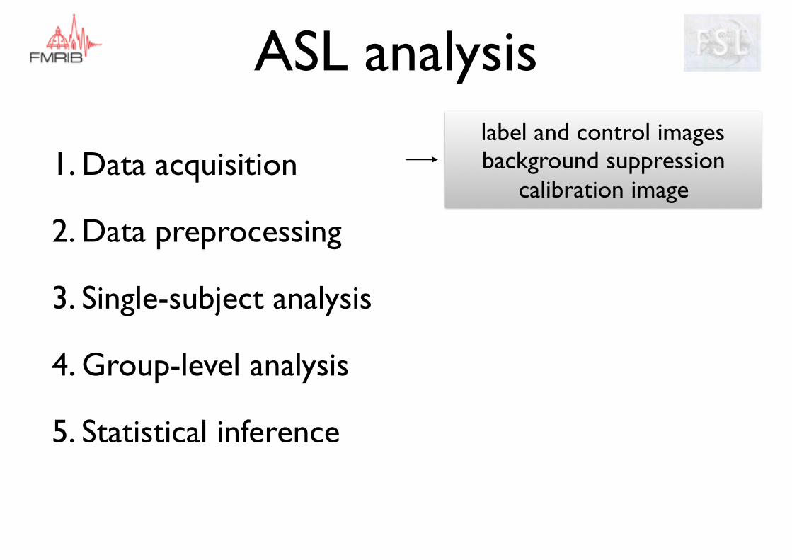
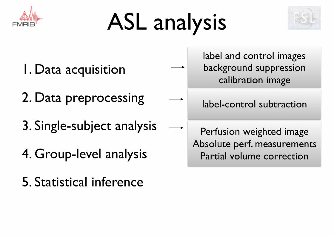
ASL analysis
1. Data acquisition
2. Data preprocessing
3. Single-subject analysis
4. Group-level analysis
5. Statistical inference
label and control imagesbackground suppression
calibration image
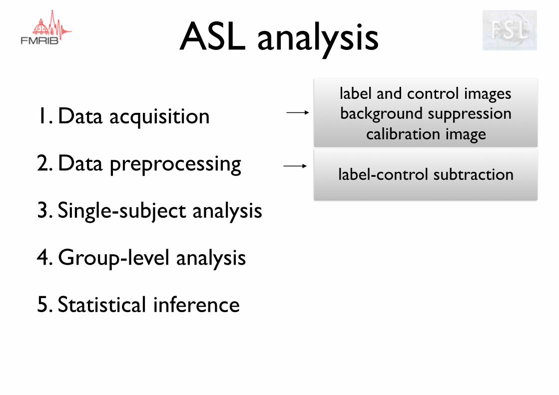
ASL analysis
1. Data acquisition
2. Data preprocessing
3. Single-subject analysis
4. Group-level analysis
5. Statistical inference
label-control subtraction
label and control imagesbackground suppression
calibration image
ASL analysis
1. Data acquisition
2. Data preprocessing
3. Single-subject analysis
4. Group-level analysis
5. Statistical inference
label-control subtraction
Perfusion weighted imageAbsolute perf. measurements
Partial volume correction
label and control imagesbackground suppression
calibration image
Advanced preprocessing
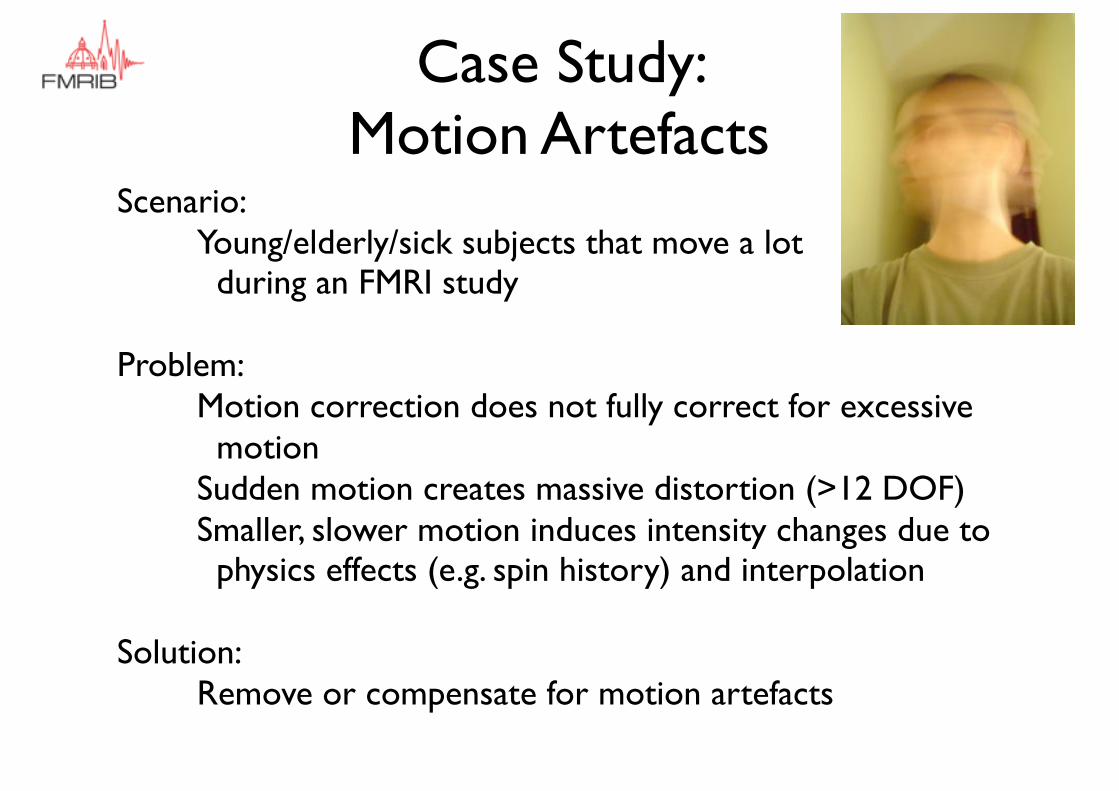
Case Study: Motion Artefacts
Scenario:Young/elderly/sick subjects that move a lot during an FMRI study
Problem:Motion correction does not fully correct for excessive motionSudden motion creates massive distortion (>12 DOF)Smaller, slower motion induces intensity changes due to physics effects (e.g. spin history) and interpolation
Solution:Remove or compensate for motion artefacts
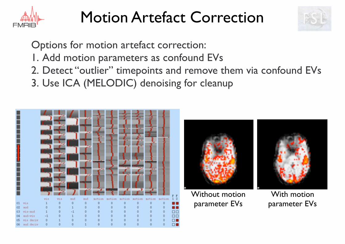
Motion Artefact Correction
Options for motion artefact correction:1. Add motion parameters as confound EVs2. Detect “outlier” timepoints and remove them via confound EVs 3. Use ICA (MELODIC) denoising for cleanup
Without motion parameter EVs
With motion parameter EVs
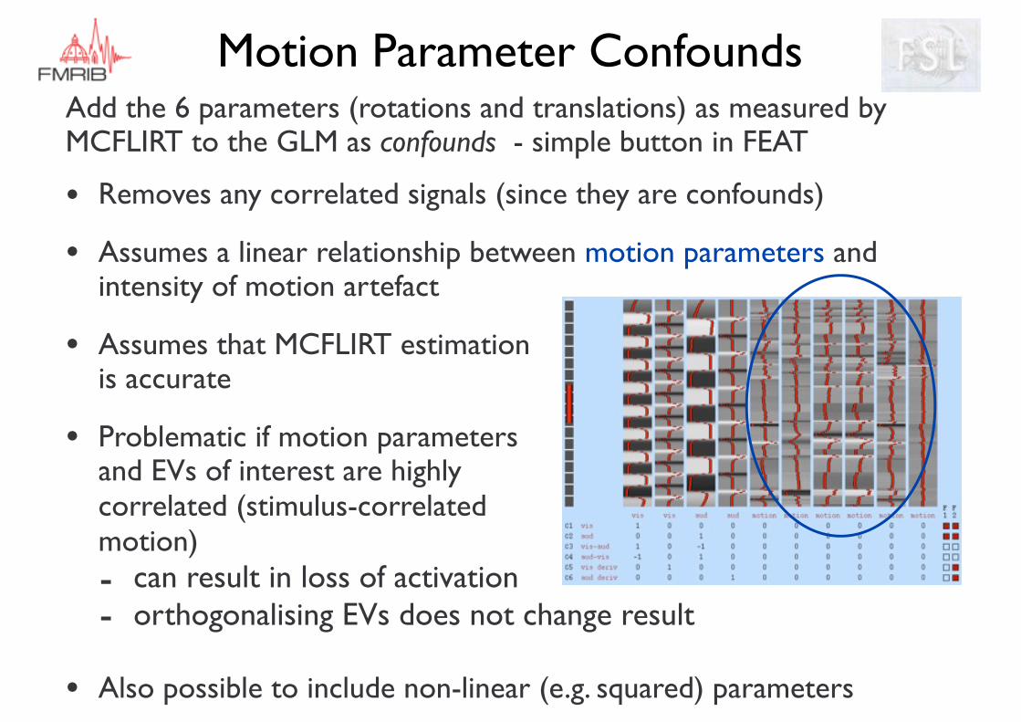
Motion Parameter ConfoundsAdd the 6 parameters (rotations and translations) as measured by MCFLIRT to the GLM as confounds - simple button in FEAT
• Removes any correlated signals (since they are confounds)
• Assumes a linear relationship between motion parameters and intensity of motion artefact
• Assumes that MCFLIRT estimation is accurate
• Problematic if motion parameters and EVs of interest are highly correlated (stimulus-correlated motion)- can result in loss of activation- orthogonalising EVs does not change result
• Also possible to include non-linear (e.g. squared) parameters
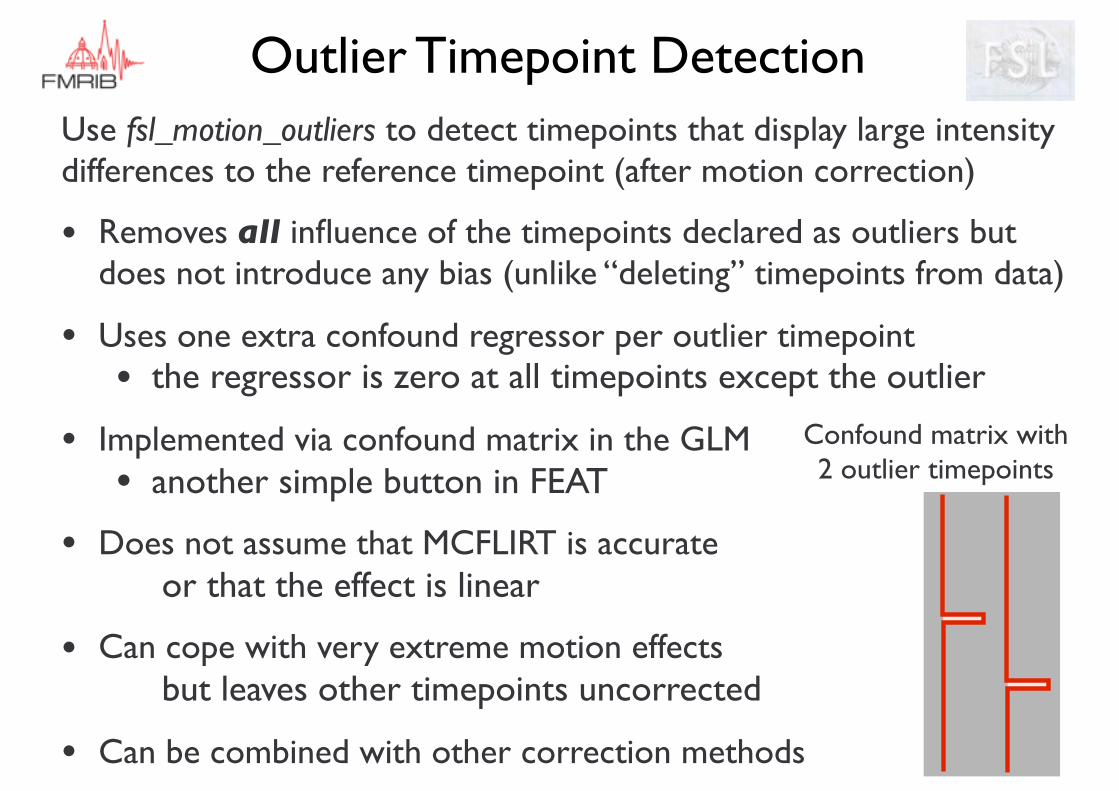
Use fsl_motion_outliers to detect timepoints that display large intensity differences to the reference timepoint (after motion correction)
• Removes all influence of the timepoints declared as outliers but does not introduce any bias (unlike “deleting” timepoints from data)
• Uses one extra confound regressor per outlier timepoint• the regressor is zero at all timepoints except the outlier
• Implemented via confound matrix in the GLM• another simple button in FEAT
• Does not assume that MCFLIRT is accurate or that the effect is linear
• Can cope with very extreme motion effects but leaves other timepoints uncorrected
• Can be combined with other correction methods
Outlier Timepoint Detection
Confound matrix with 2 outlier timepoints
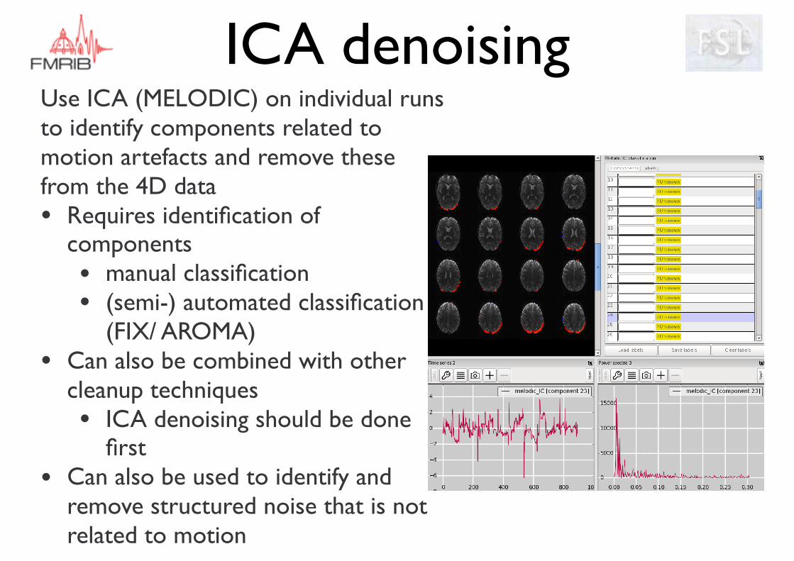
ICA denoisingUse ICA (MELODIC) on individual runs to identify components related to motion artefacts and remove these from the 4D data• Requires identification of
components • manual classification • (semi-) automated classification
(FIX/ AROMA)• Can also be combined with other
cleanup techniques• ICA denoising should be done
first• Can also be used to identify and
remove structured noise that is not related to motion
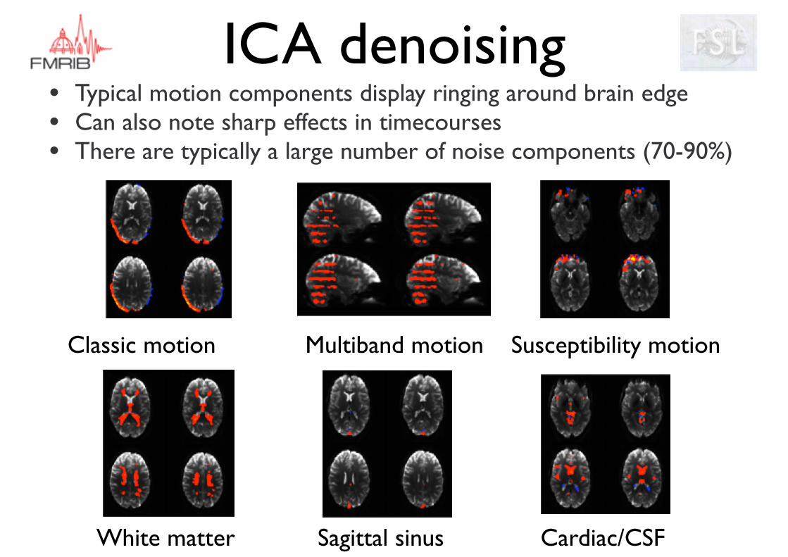
• Typical motion components display ringing around brain edge• Can also note sharp effects in timecourses• There are typically a large number of noise components (70-90%)
ICA denoising
Classic motion Multiband motion Susceptibility motion
White matter Sagittal sinus Cardiac/CSF
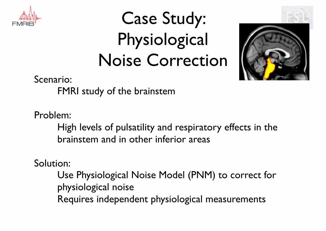
Case Study: Physiological
Noise CorrectionScenario:
FMRI study of the brainstem
Problem:High levels of pulsatility and respiratory effects in the brainstem and in other inferior areas
Solution:Use Physiological Noise Model (PNM) to correct for physiological noiseRequires independent physiological measurements
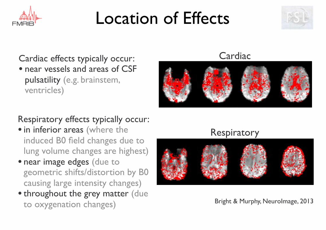
Location of Effects
Cardiac effects typically occur:• near vessels and areas of CSF
pulsatility (e.g. brainstem, ventricles)
Cardiac
Respiratory
Bright & Murphy, NeuroImage, 2013
Respiratory effects typically occur:• in inferior areas (where the
induced B0 field changes due to lung volume changes are highest)
• near image edges (due to geometric shifts/distortion by B0 causing large intensity changes)
• throughout the grey matter (due to oxygenation changes)
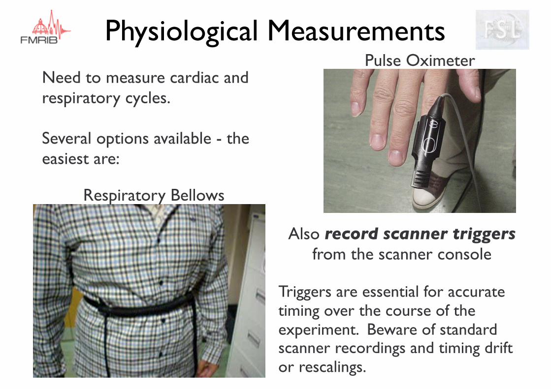
Physiological MeasurementsPulse Oximeter
Respiratory Bellows
Need to measure cardiac and respiratory cycles.
Several options available - the easiest are:
Also record scanner triggersfrom the scanner console
Triggers are essential for accurate timing over the course of the experiment. Beware of standard scanner recordings and timing drift or rescalings.
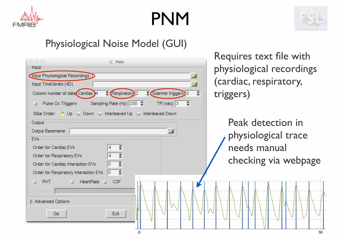
PNMPhysiological Noise Model (GUI)
Requires text file with physiological recordings (cardiac, respiratory, triggers)
Peak detection in physiological trace needs manual checking via webpage
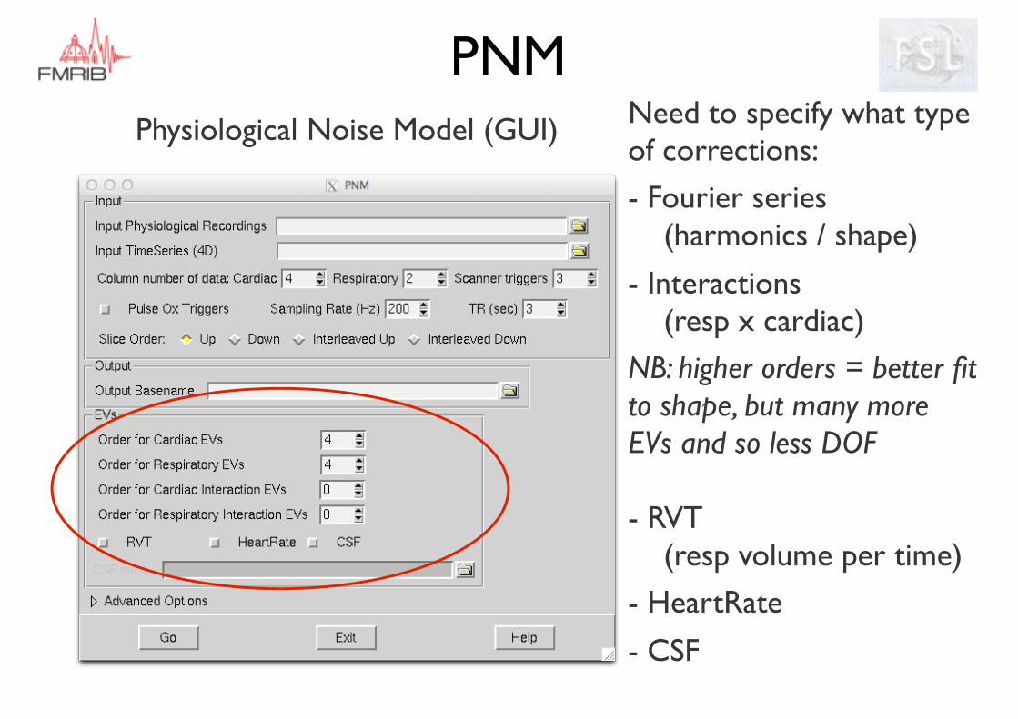
PNMPhysiological Noise Model (GUI) Need to specify what type
of corrections:
- Fourier series (harmonics / shape)
- Interactions (resp x cardiac)
NB: higher orders = better fit to shape, but many more EVs and so less DOF
- RVT (resp volume per time)
- HeartRate
- CSF
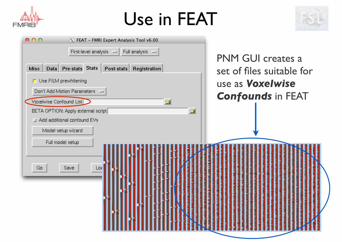
Use in FEAT
PNM GUI creates a set of files suitable for use as Voxelwise Confounds in FEAT
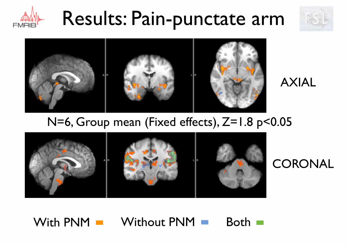
Results: Pain-punctate arm
N=6, Group mean (Fixed effects), Z=1.8 p<0.05
AXIAL
CORONAL
With PNM Without PNM Both
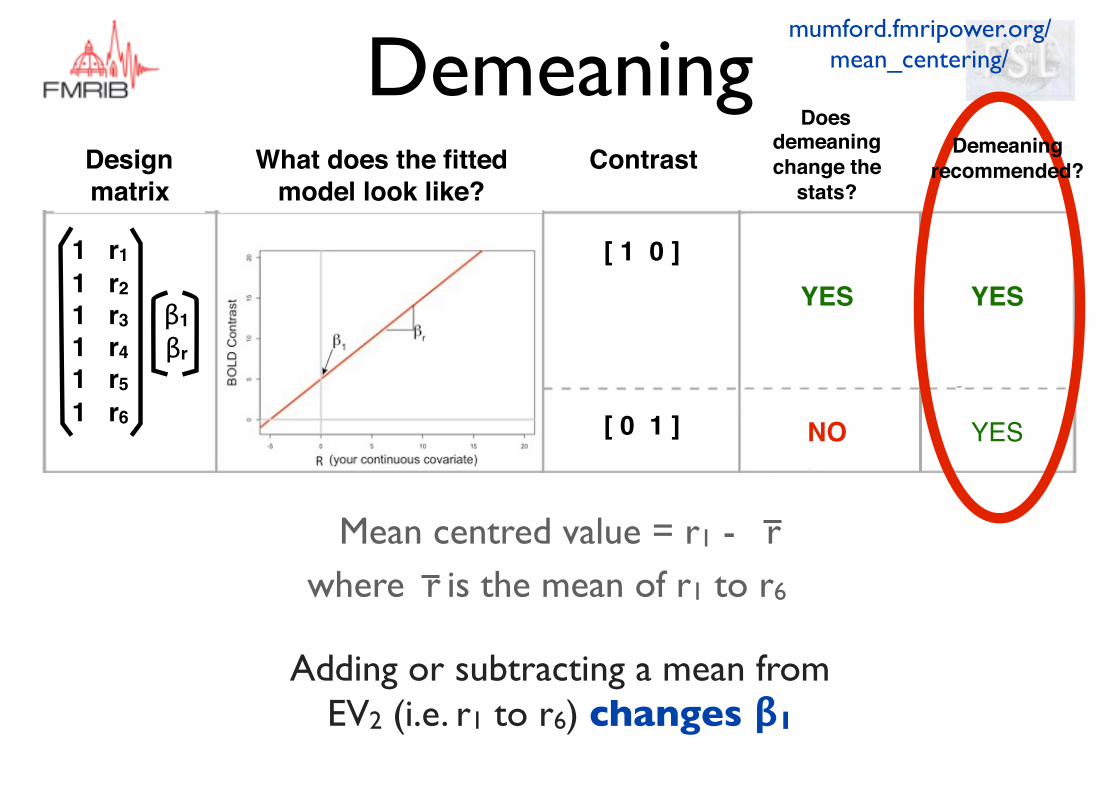
Demeaning EVs
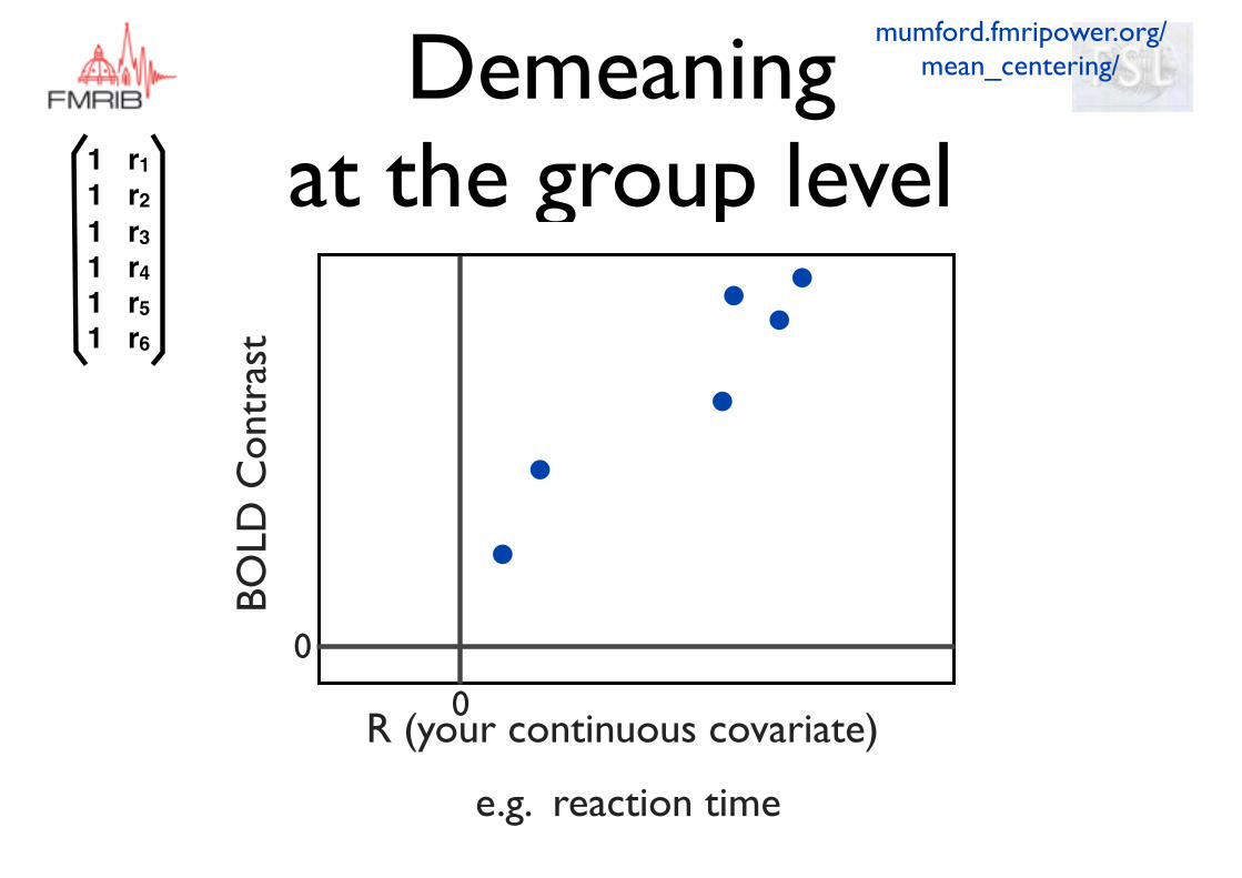
Demeaning at the group level
BOLD
Con
tras
t
R (your continuous covariate)
e.g. reaction time
mumford.fmripower.org/mean_centering/
0
0
1 r11 r21 r31 r41 r51 r6
BOLD
Con
tras
t
R (your continuous covariate)
e.g. reaction time
mumford.fmripower.org/mean_centering/
0
0
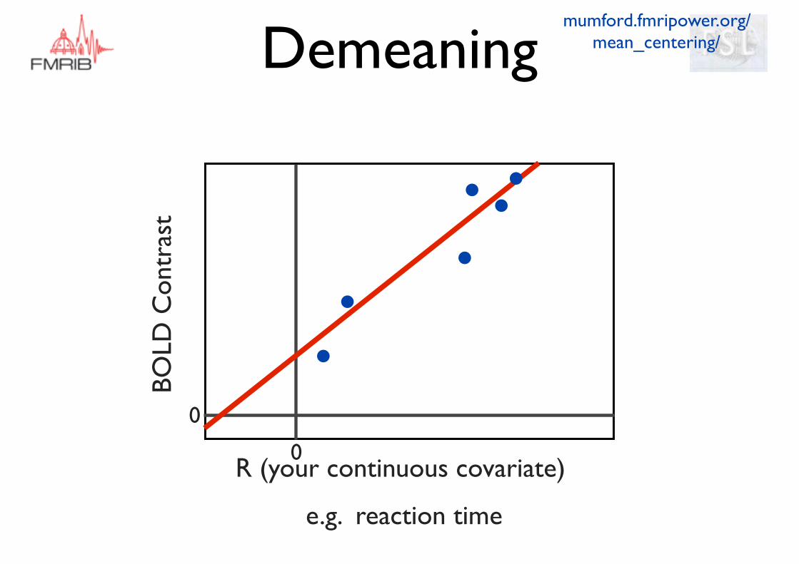
Demeaning
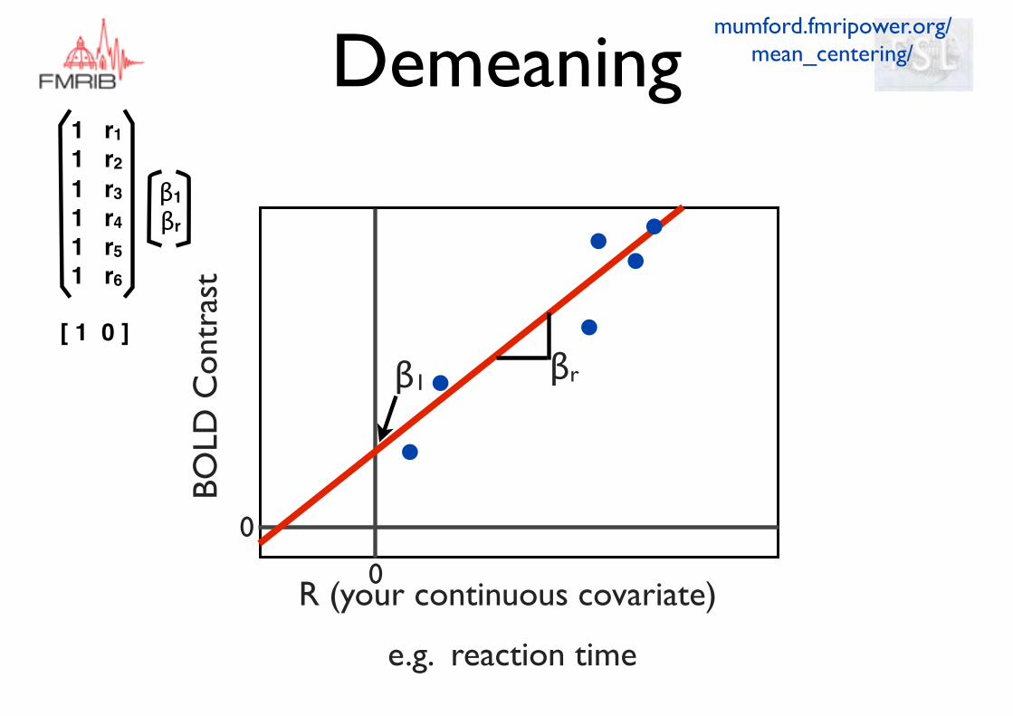
BOLD
Con
tras
t
R (your continuous covariate)
βrβ1
e.g. reaction time
mumford.fmripower.org/mean_centering/
0
0
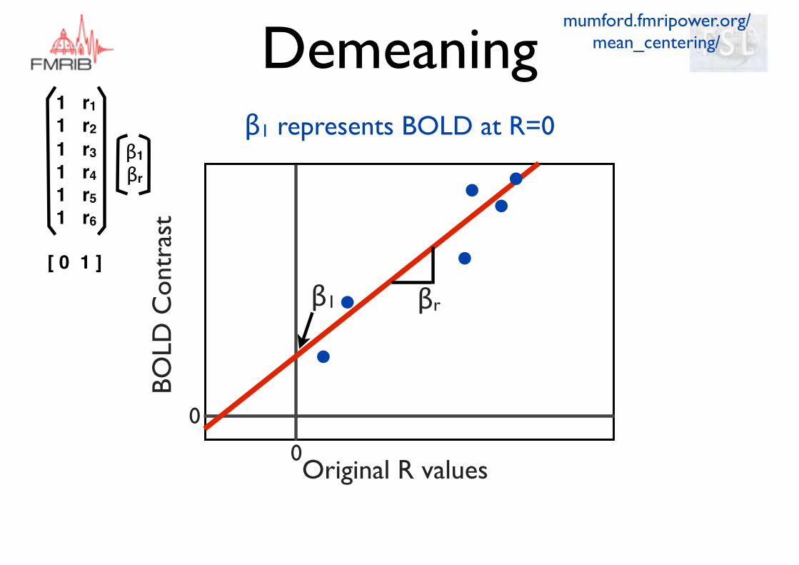
Demeaning
β1βr
1 r11 r21 r31 r41 r51 r6
[ 1 0 ]
BOLD
Con
tras
t
Demeaned R values
βr
β1
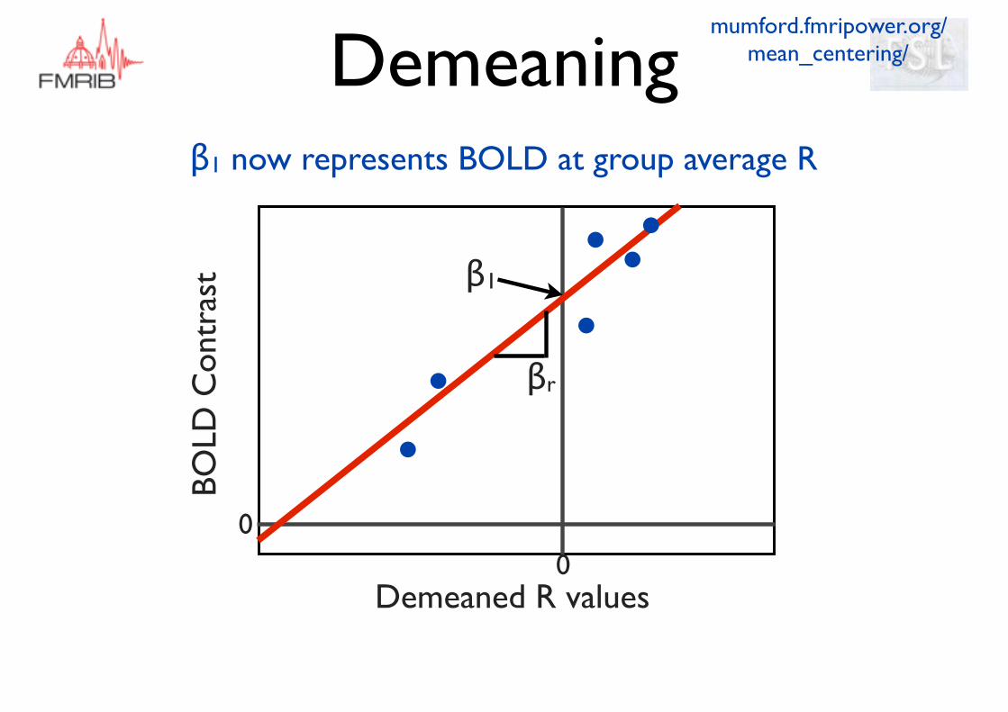
mumford.fmripower.org/mean_centering/
00
β1 now represents BOLD at group average R
Demeaning
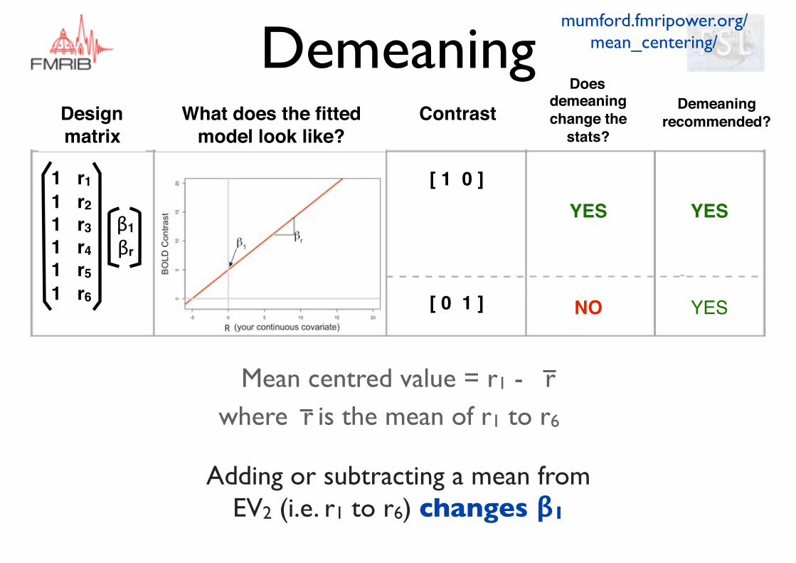
Does demeaning change the
stats?What does the fitted
model look like?ContrastDesign
matrix
[ 1 0 ]
[ 0 1 ]
1 r11 r21 r31 r41 r51 r6
β1βr
Mean centred value = r1 - rwhere is the mean of r1 to r6r
YES
NO
YES
YES
Adding or subtracting a mean from EV2 (i.e. r1 to r6) changes β1
mumford.fmripower.org/mean_centering/
Demeaning recommended?
Demeaning
BOLD
Con
tras
t
Original R values
β1
mumford.fmripower.org/mean_centering/
0
0
βr
β1 represents BOLD at R=0
Demeaning
β1βr
1 r11 r21 r31 r41 r51 r6
[ 0 1 ]

BOLD
Con
tras
t
Demeaned R values
βr
β1
mumford.fmripower.org/mean_centering/
00
β1 now represents BOLD at group average R
Demeaning
Does demeaning change the
stats?What does the fitted
model look like?ContrastDesign
matrix
[ 1 0 ]
[ 0 1 ]
1 r11 r21 r31 r41 r51 r6
β1βr
Mean centred value = r1 - rwhere is the mean of r1 to r6r
YES
NO
YES
YES
Adding or subtracting a mean from EV2 (i.e. r1 to r6) changes β1
mumford.fmripower.org/mean_centering/
Demeaning recommended?
Demeaning

Advanced designs
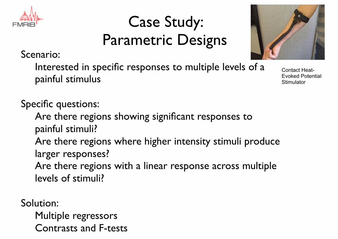
Case Study: Parametric Designs
Scenario: Interested in specific responses to multiple levels of a painful stimulus
Specific questions:Are there regions showing significant responses to painful stimuli?Are there regions where higher intensity stimuli produce larger responses?Are there regions with a linear response across multiple levels of stimuli?
Solution:Multiple regressorsContrasts and F-tests
Contact Heat-Evoked Potential Stimulator
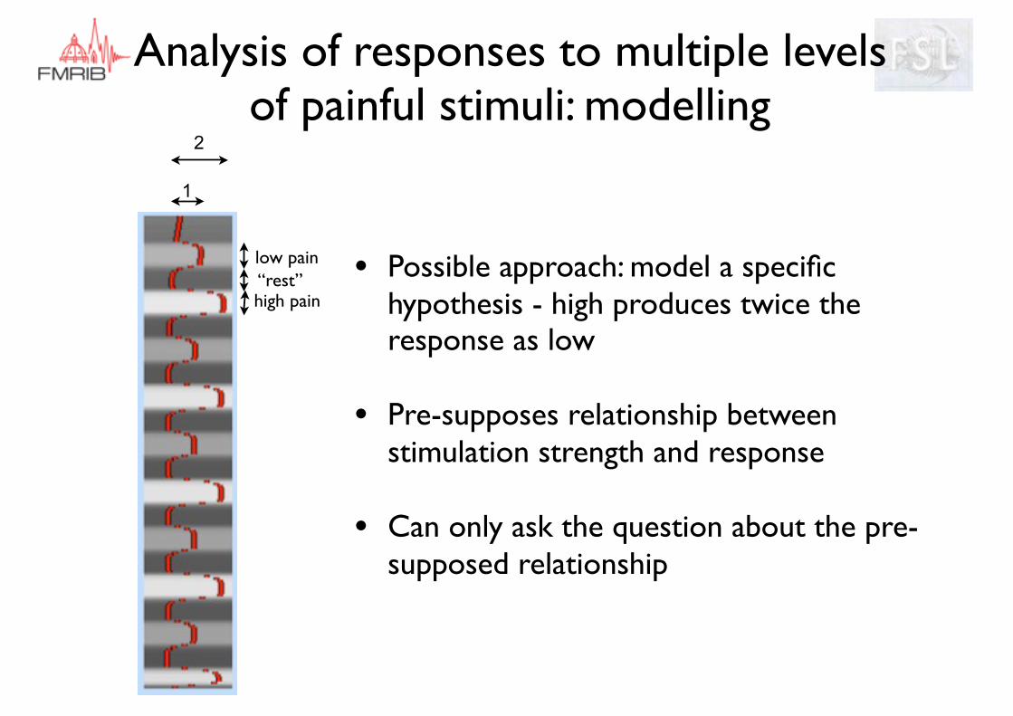
• Possible approach: model a specific hypothesis - high produces twice the response as low
• Pre-supposes relationship between stimulation strength and response
• Can only ask the question about the pre-supposed relationship
low pain“rest”high pain
1
2
Analysis of responses to multiple levels of painful stimuli: modelling
• Can assess responses to individual stimuli
• t-contrast [0 1]: “ response to low pain”
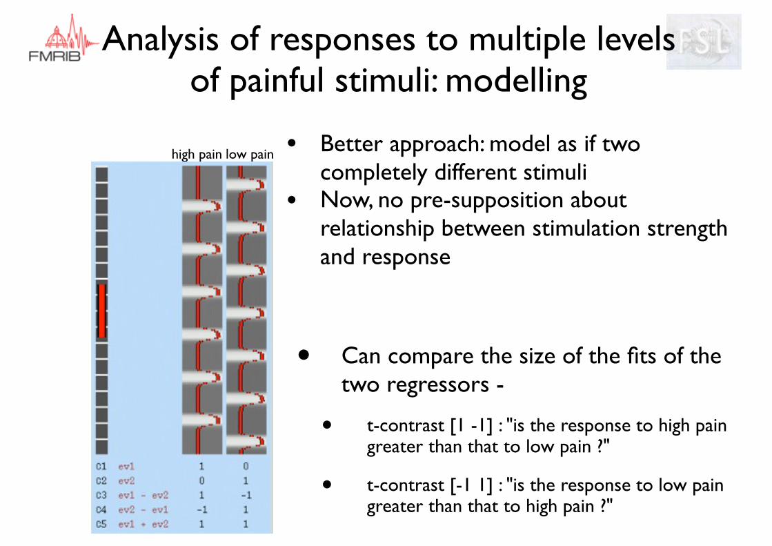
• Better approach: model as if two completely different stimuli
• Now, no pre-supposition about relationship between stimulation strength and response
low painhigh pain
Analysis of responses to multiple levels of painful stimuli: modelling
• Better approach: model as if two completely different stimuli
• Now, no pre-supposition about relationship between stimulation strength and response
low painhigh pain
• Can compare the size of the fits of the two regressors -
• t-contrast [1 -1] : "is the response to high pain greater than that to low pain ?"
• t-contrast [-1 1] : "is the response to low pain greater than that to high pain ?"
Analysis of responses to multiple levels of painful stimuli: modelling

• Average response?
• t-contrast [1 1] : "is the average response to pain greater than zero?"
• Better approach: model as if two completely different stimuli
• Now, no pre-supposition about relationship between stimulation strength and response
low painhigh pain
Analysis of responses to multiple levels of painful stimuli: modelling
Parametric Variation - Linear Trends
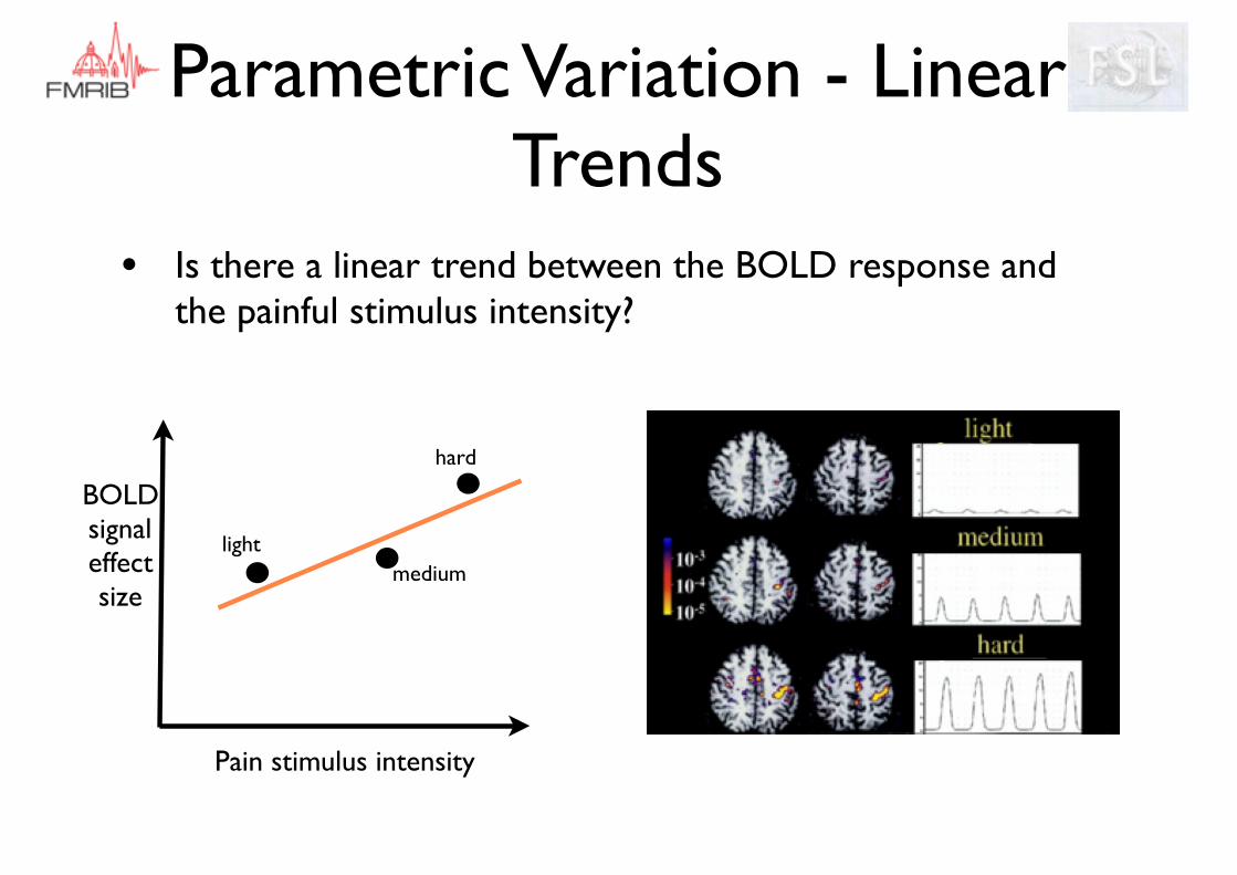
• Is there a linear trend between the BOLD response and the painful stimulus intensity?
BOLD signal effect size
Pain stimulus intensity
lightmedium
hard
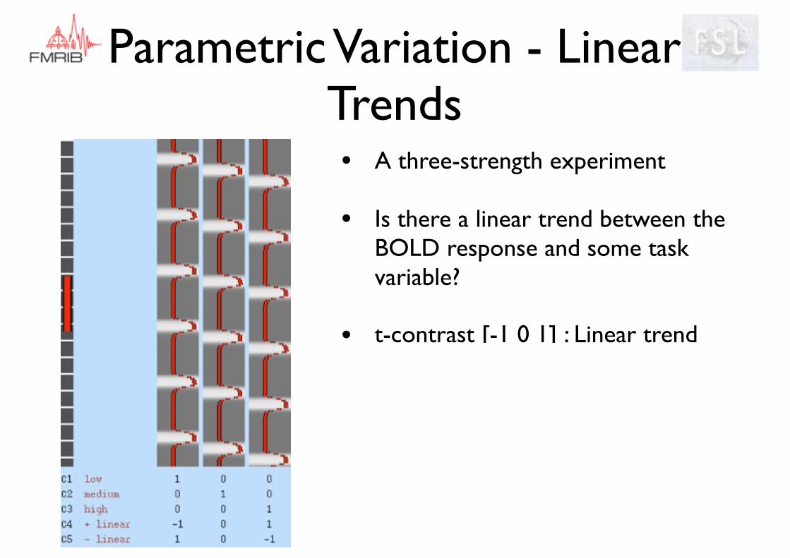
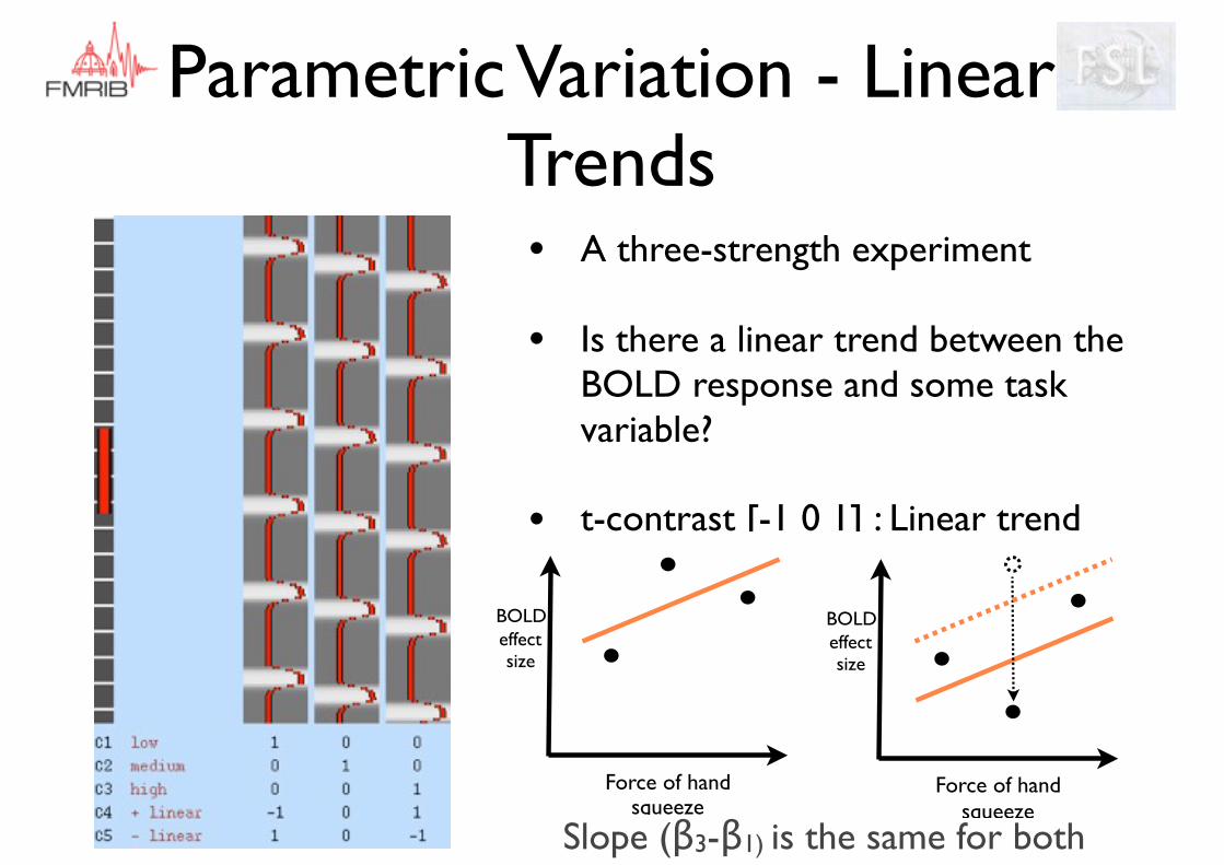
• A three-strength experiment
• Is there a linear trend between the BOLD response and some task variable?
• t-contrast [-1 0 1] : Linear trend
Parametric Variation - Linear Trends
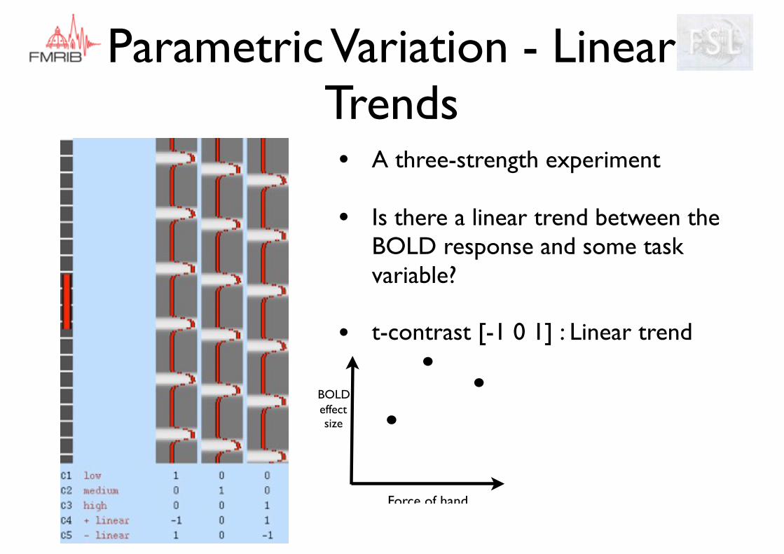
• A three-strength experiment
• Is there a linear trend between the BOLD response and some task variable?
• t-contrast [-1 0 1] : Linear trend
BOLDeffect size
Force of hand
Parametric Variation - Linear Trends
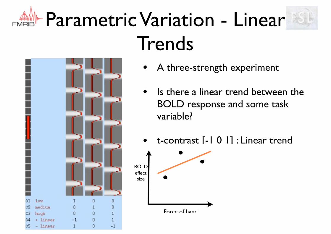
• A three-strength experiment
• Is there a linear trend between the BOLD response and some task variable?
• t-contrast [-1 0 1] : Linear trend
BOLDeffect size
Force of hand
Parametric Variation - Linear Trends
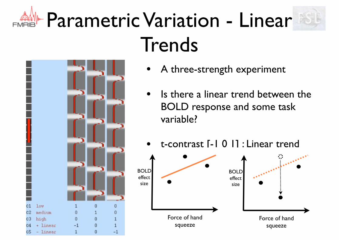
• A three-strength experiment
• Is there a linear trend between the BOLD response and some task variable?
• t-contrast [-1 0 1] : Linear trend
BOLDeffect size
Force of hand squeeze
BOLDeffect size
Force of hand squeeze
Parametric Variation - Linear Trends
Parametric Variation - Linear Trends• A three-strength experiment
• Is there a linear trend between the BOLD response and some task variable?
• t-contrast [-1 0 1] : Linear trend
BOLDeffect size
Force of hand squeeze
BOLDeffect size
Force of hand squeeze
Slope (β3-β1) is the same for both
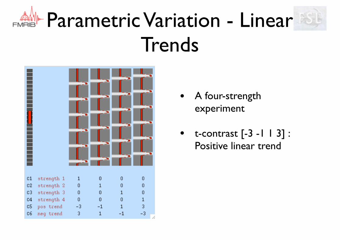
• A four-strength experiment
• t-contrast [-3 -1 1 3] : Positive linear trend
Parametric Variation - Linear Trends
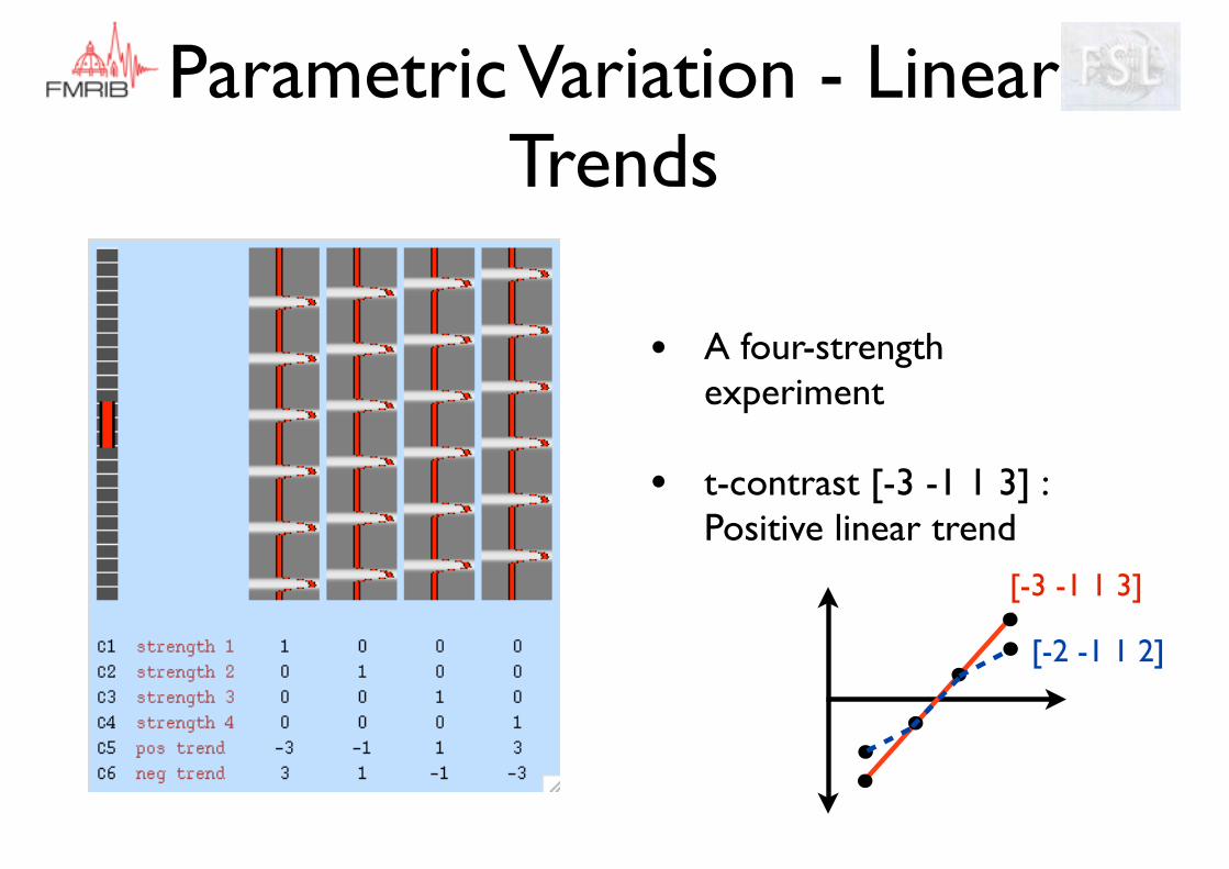
• A four-strength experiment
• t-contrast [-3 -1 1 3] : Positive linear trend
Parametric Variation - Linear Trends
[-3 -1 1 3]
[-2 -1 1 2]
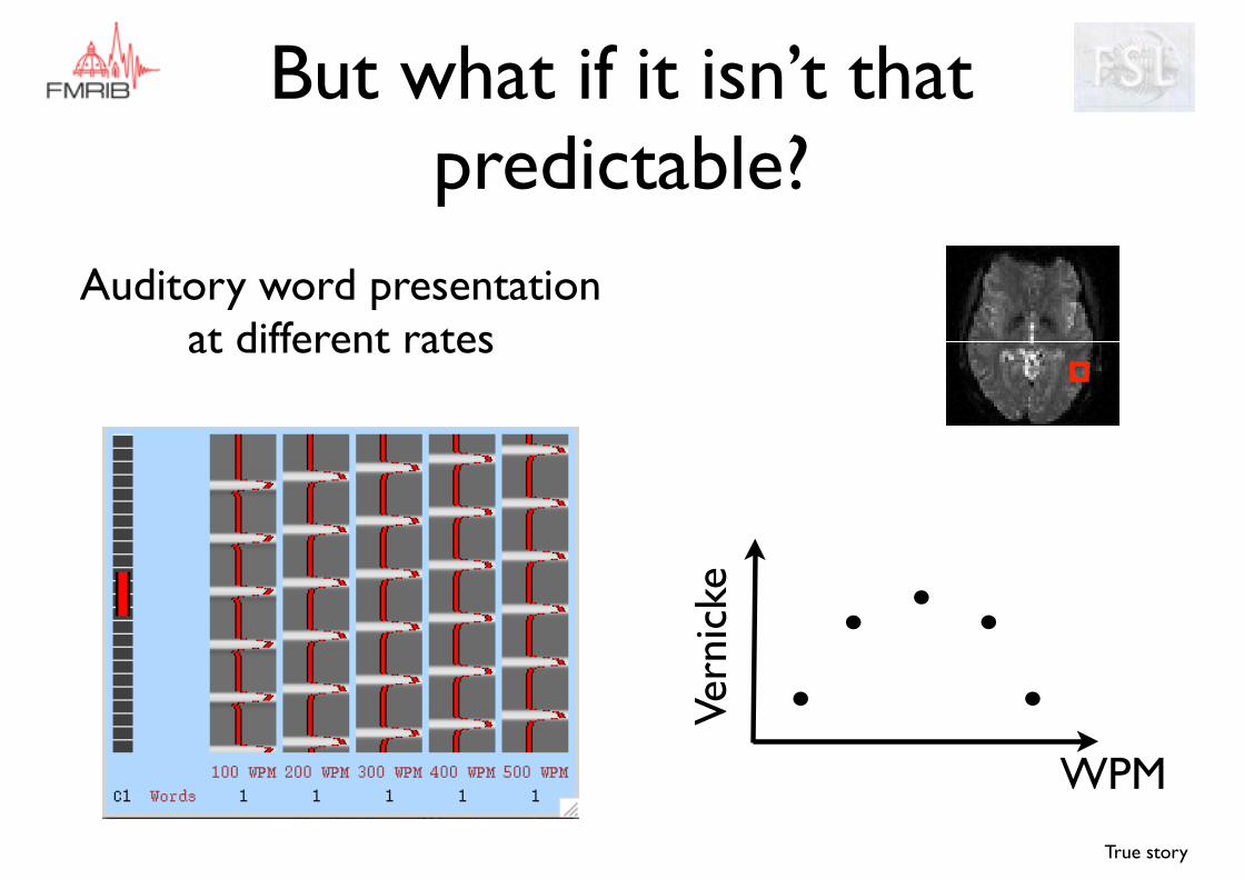
But what if it isn’t that predictable?
Auditory word presentation at different rates
WPM
True story
Vern
icke
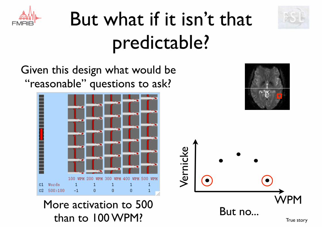
But what if it isn’t that predictable?
Given this design what would be “reasonable” questions to ask?
True story
WPMVe
rnic
ke
More activation to 500 than to 100 WPM? But no...

But what if it isn’t that predictable?
Given this design what would be “reasonable” questions to ask?
True story
WPMVe
rnic
ke
Activation proportional to WPM? Still no...
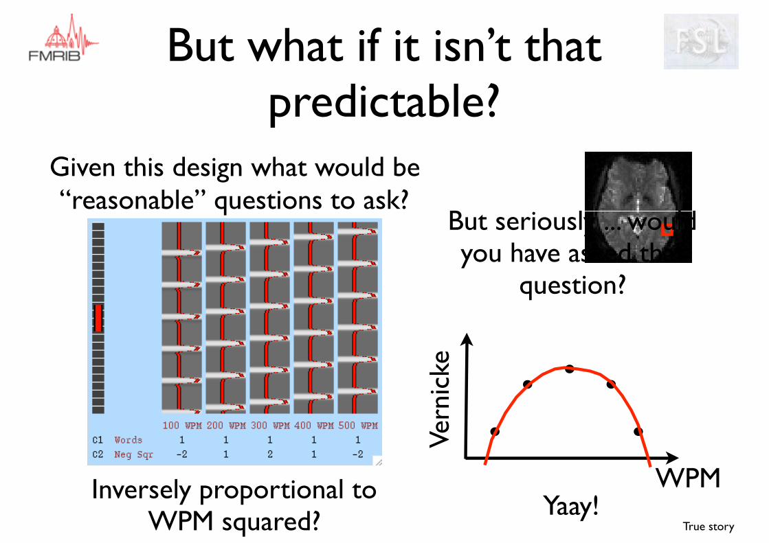
But what if it isn’t that predictable?
Given this design what would be “reasonable” questions to ask?
True story
WPMVe
rnic
ke
Inversely proportional to WPM squared? Yaay!
But seriously ... would you have asked that
question?
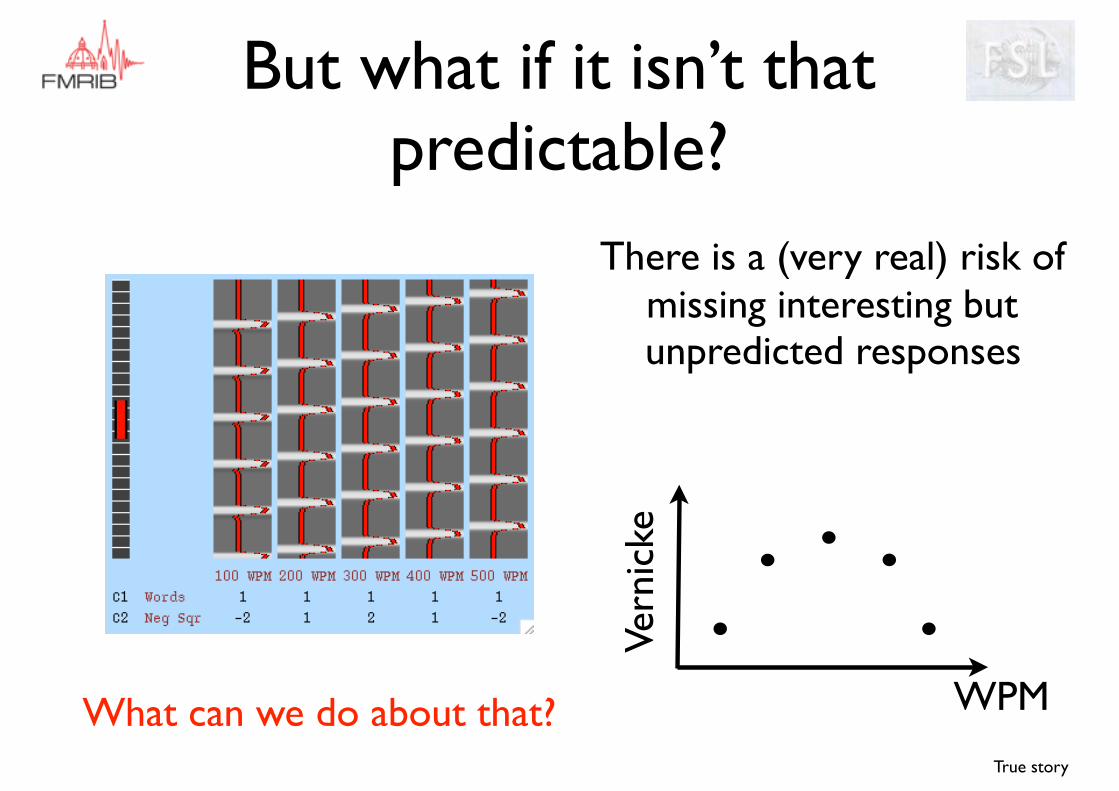
But what if it isn’t that predictable?
True story
WPMVe
rnic
ke
There is a (very real) risk of missing interesting but unpredicted responses
What can we do about that?
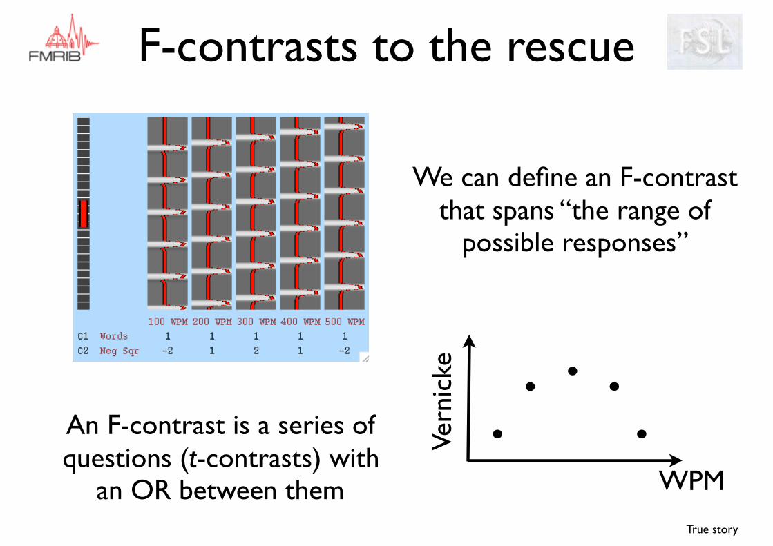
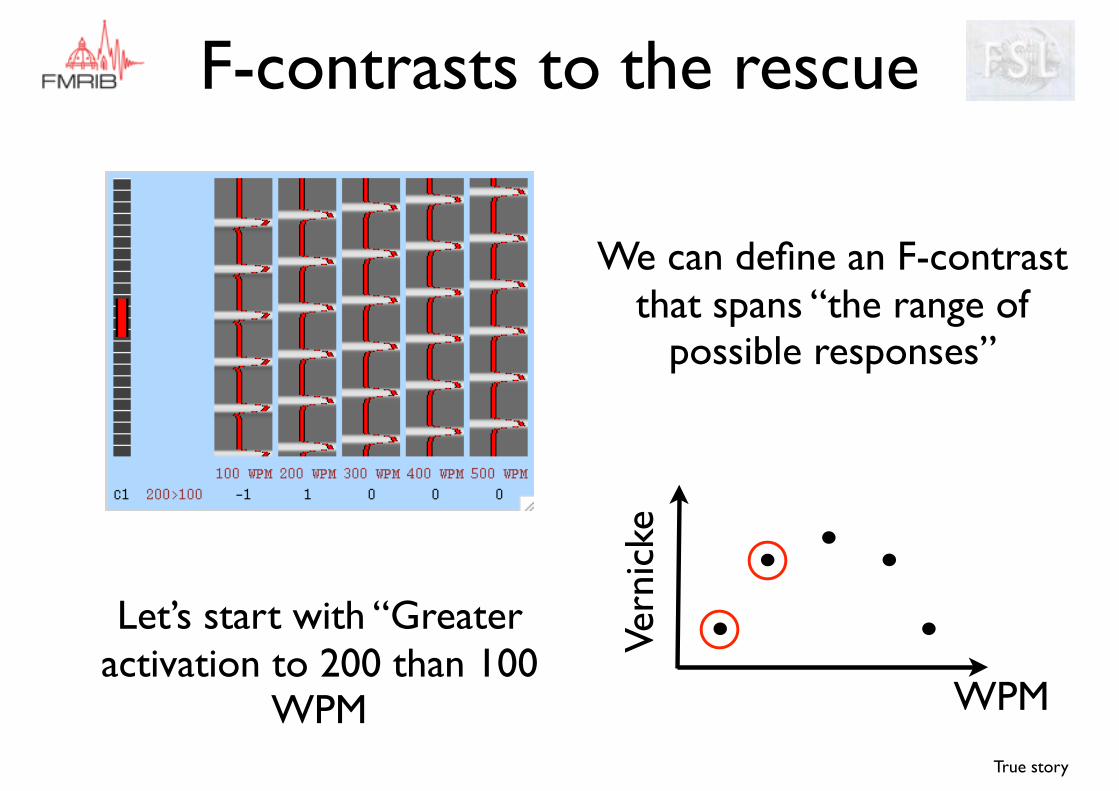
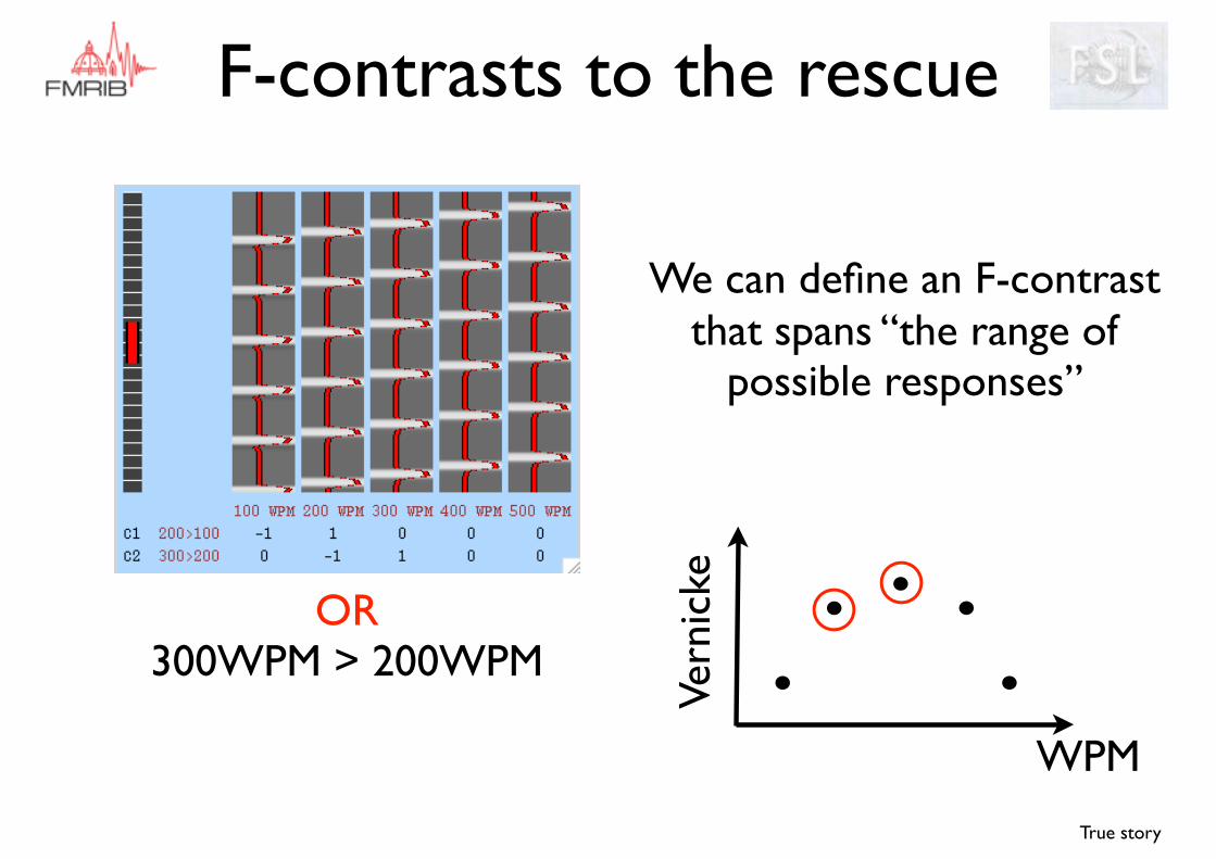
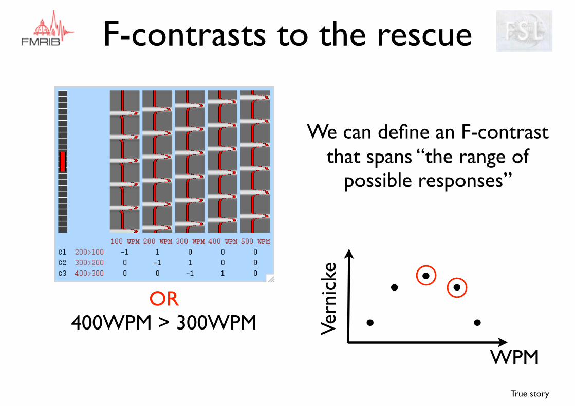
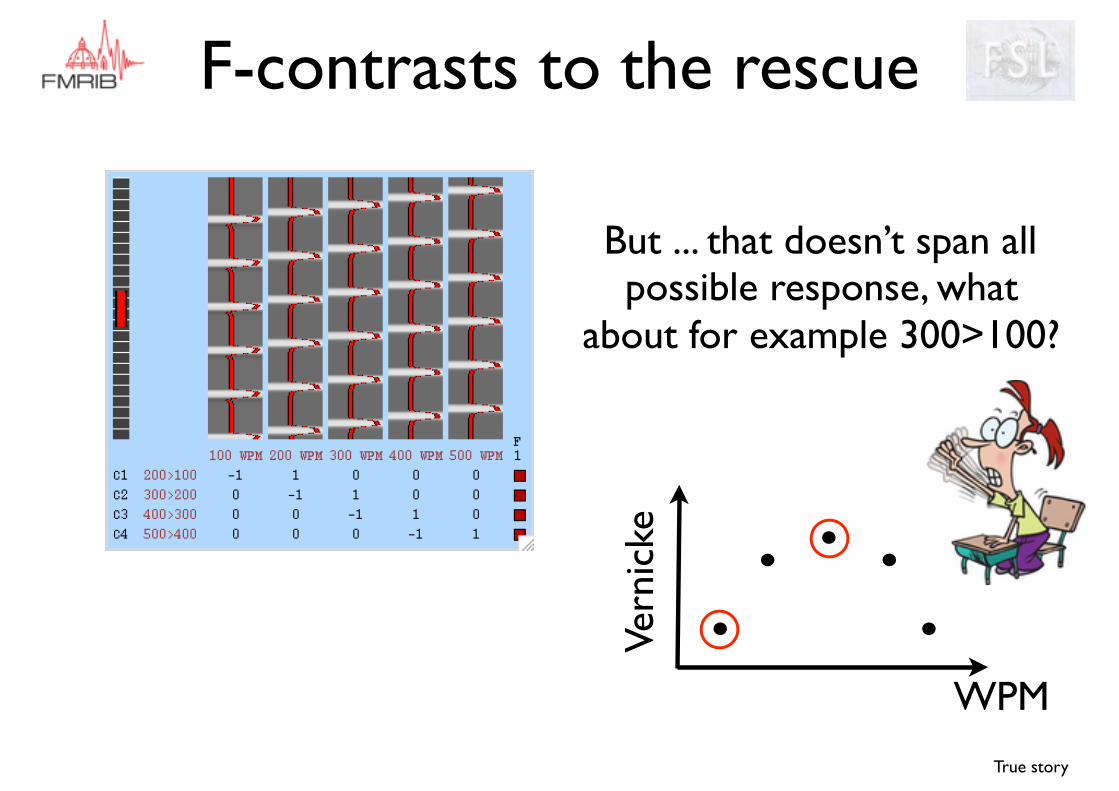
F-contrasts to the rescue
True story
WPMVe
rnic
ke
We can define an F-contrast that spans “the range of
possible responses”
An F-contrast is a series of questions (t-contrasts) with
an OR between them
F-contrasts to the rescue
True story
WPMVe
rnic
ke
We can define an F-contrast that spans “the range of
possible responses”
Let’s start with “Greater activation to 200 than 100
WPM
F-contrasts to the rescue
True story
WPMVe
rnic
ke
We can define an F-contrast that spans “the range of
possible responses”
OR300WPM > 200WPM
F-contrasts to the rescue
True story
WPMVe
rnic
ke
We can define an F-contrast that spans “the range of
possible responses”
OR400WPM > 300WPM
F-contrasts to the rescue
True story
WPMVe
rnic
keOR
500WPM > 400WPM
N.B.
F-contrasts to the rescue
True story
WPMVe
rnic
ke
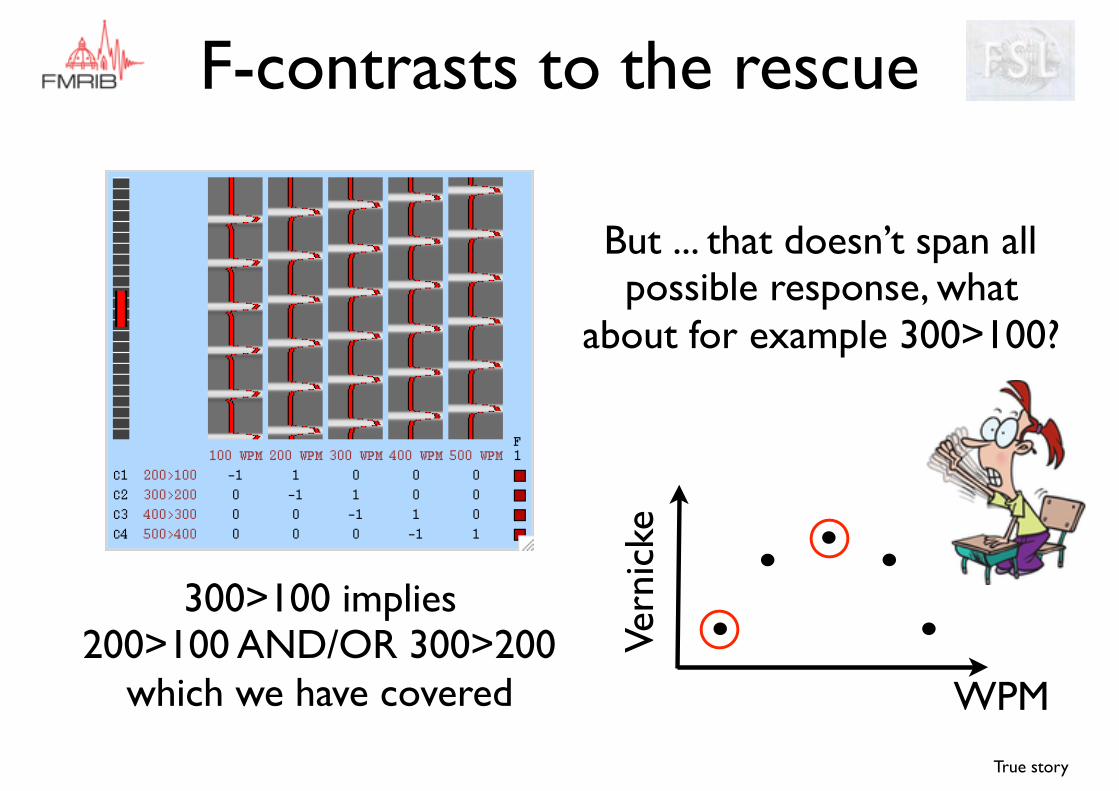
But ... that doesn’t span all possible response, what
about for example 300>100?
F-contrasts to the rescue
True story
WPMVe
rnic
ke
But ... that doesn’t span all possible response, what
about for example 300>100?
300>100 implies 200>100 AND/OR 300>200
which we have covered
F-contrasts to the rescue
True story
WPMVe
rnic
ke
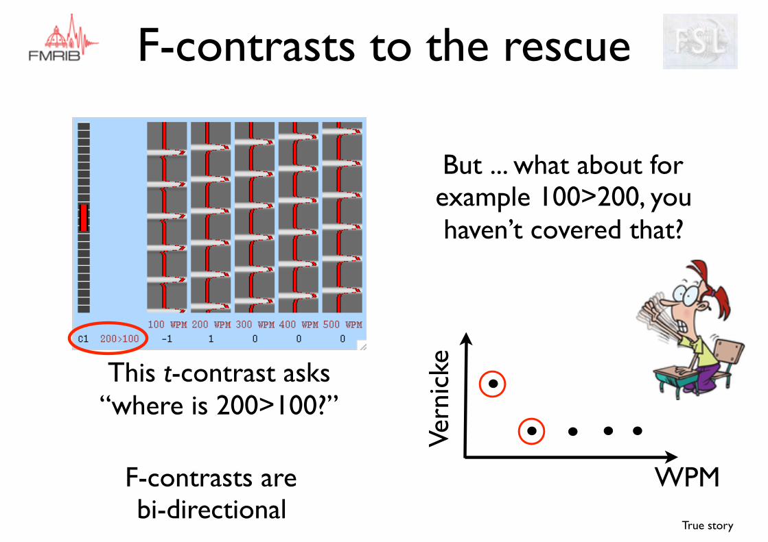
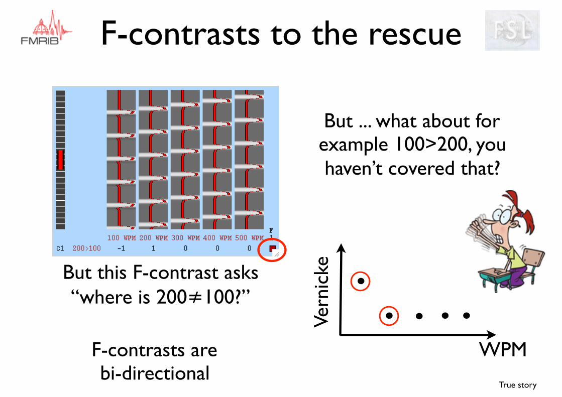
But ... what about for example 100>200, you haven’t covered that?
F-contrasts are bi-directional
This t-contrast asks “where is 200>100?”
F-contrasts to the rescue
True story
WPMVe
rnic
ke
But ... what about for example 100>200, you haven’t covered that?
F-contrasts are bi-directional
But this F-contrast asks “where is 200≠100?”
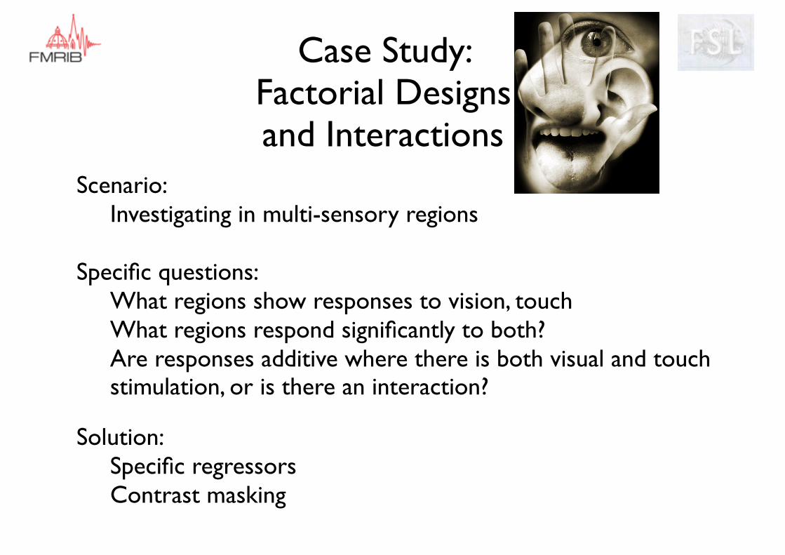
Case Study: Factorial Designs and Interactions
Scenario: Investigating in multi-sensory regions
Specific questions:What regions show responses to vision, touchWhat regions respond significantly to both?Are responses additive where there is both visual and touch stimulation, or is there an interaction?
Solution:Specific regressorsContrast masking
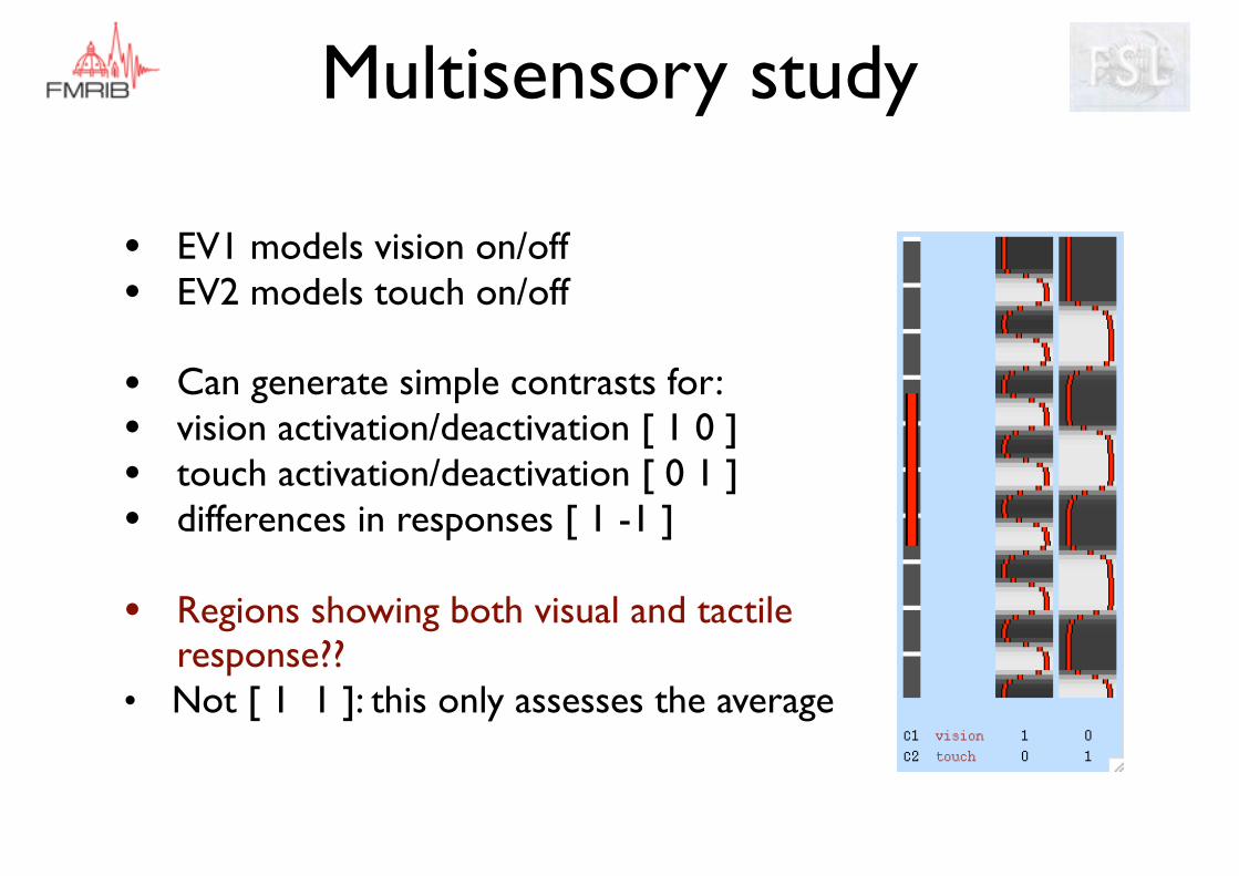
Multisensory study
• EV1 models vision on/off• EV2 models touch on/off
• Can generate simple contrasts for:• vision activation/deactivation [ 1 0 ]• touch activation/deactivation [ 0 1 ]• differences in responses [ 1 -1 ]
• Regions showing both visual and tactile response??
• Not [ 1 1 ]: this only assesses the average
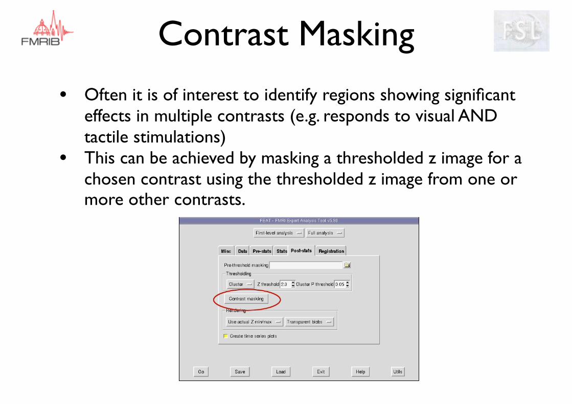
Contrast Masking
• Often it is of interest to identify regions showing significant effects in multiple contrasts (e.g. responds to visual AND tactile stimulations)
• This can be achieved by masking a thresholded z image for a chosen contrast using the thresholded z image from one or more other contrasts.
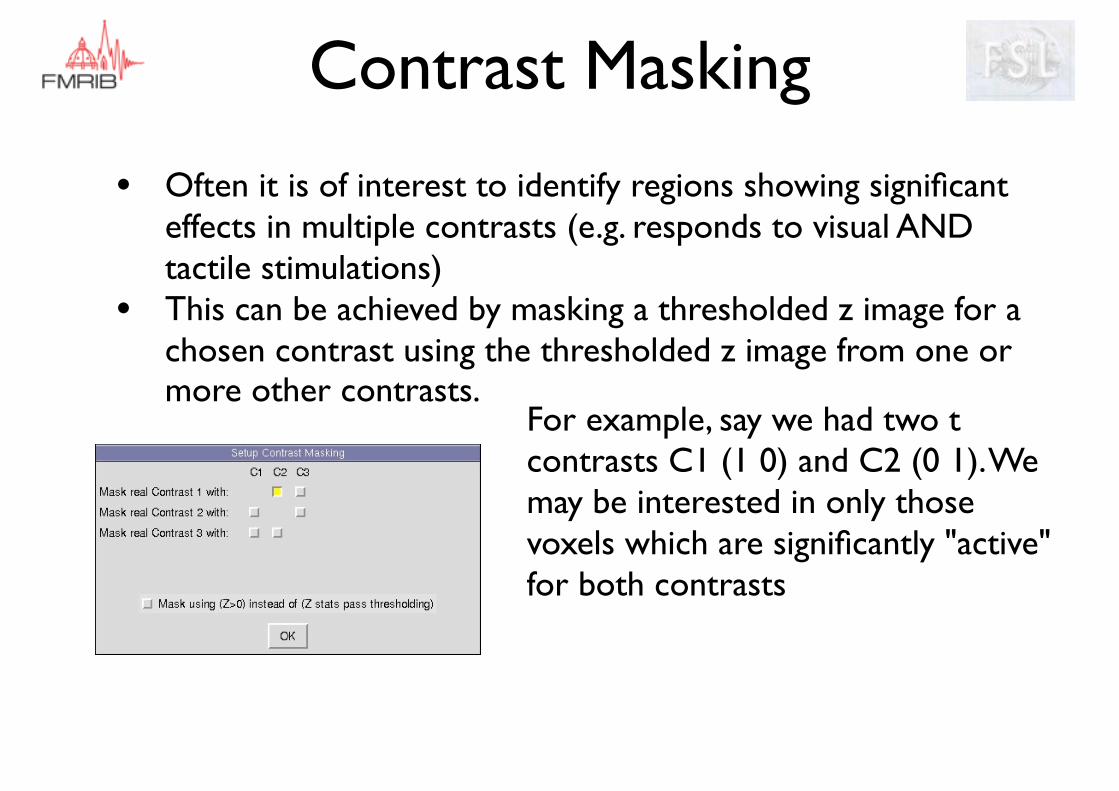
For example, say we had two t contrasts C1 (1 0) and C2 (0 1). We may be interested in only those voxels which are significantly "active" for both contrasts
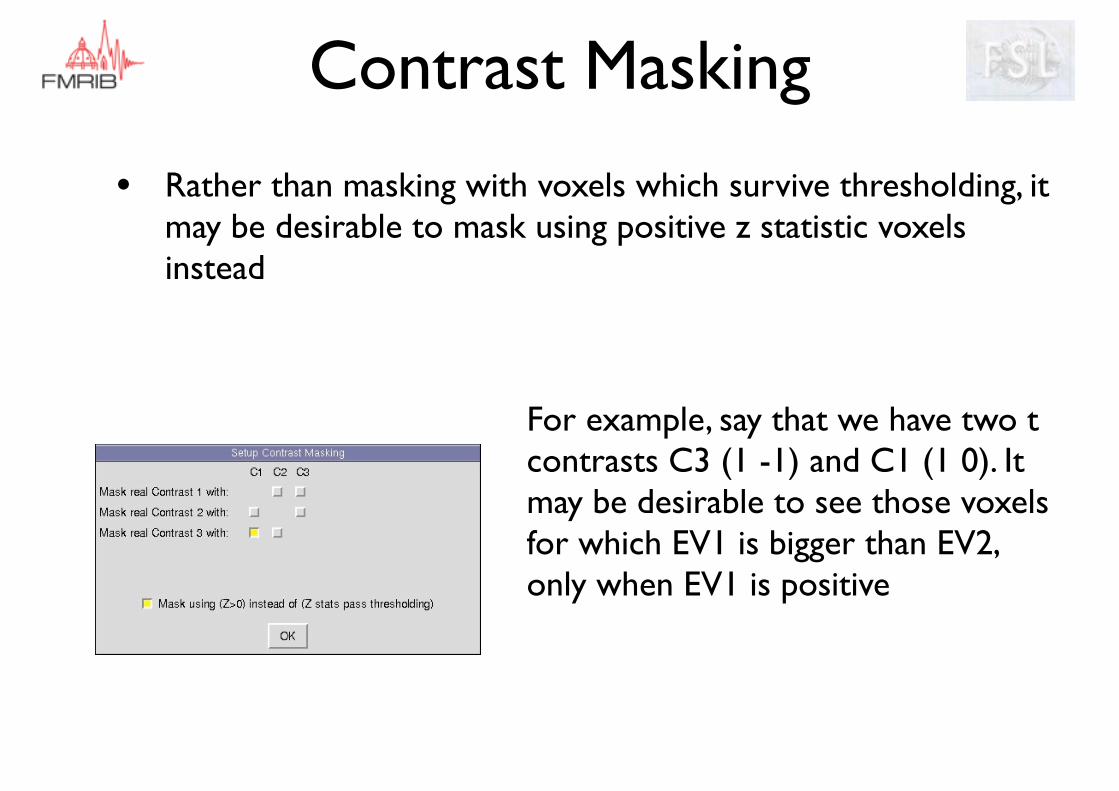
• Rather than masking with voxels which survive thresholding, it may be desirable to mask using positive z statistic voxels instead
For example, say that we have two t contrasts C3 (1 -1) and C1 (1 0). It may be desirable to see those voxels for which EV1 is bigger than EV2, only when EV1 is positive
Contrast Masking
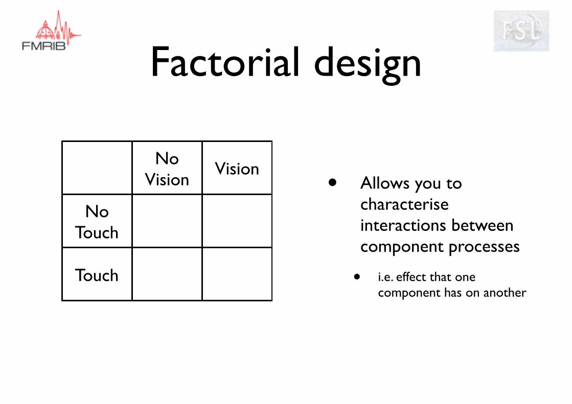
Factorial design
• Allows you to characterise interactions between component processes
• i.e. effect that one component has on another
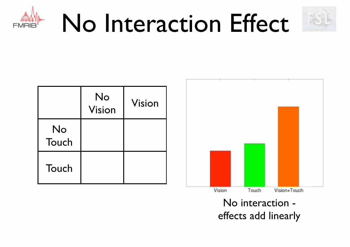
No Vision
Vision
No Touch
Touch
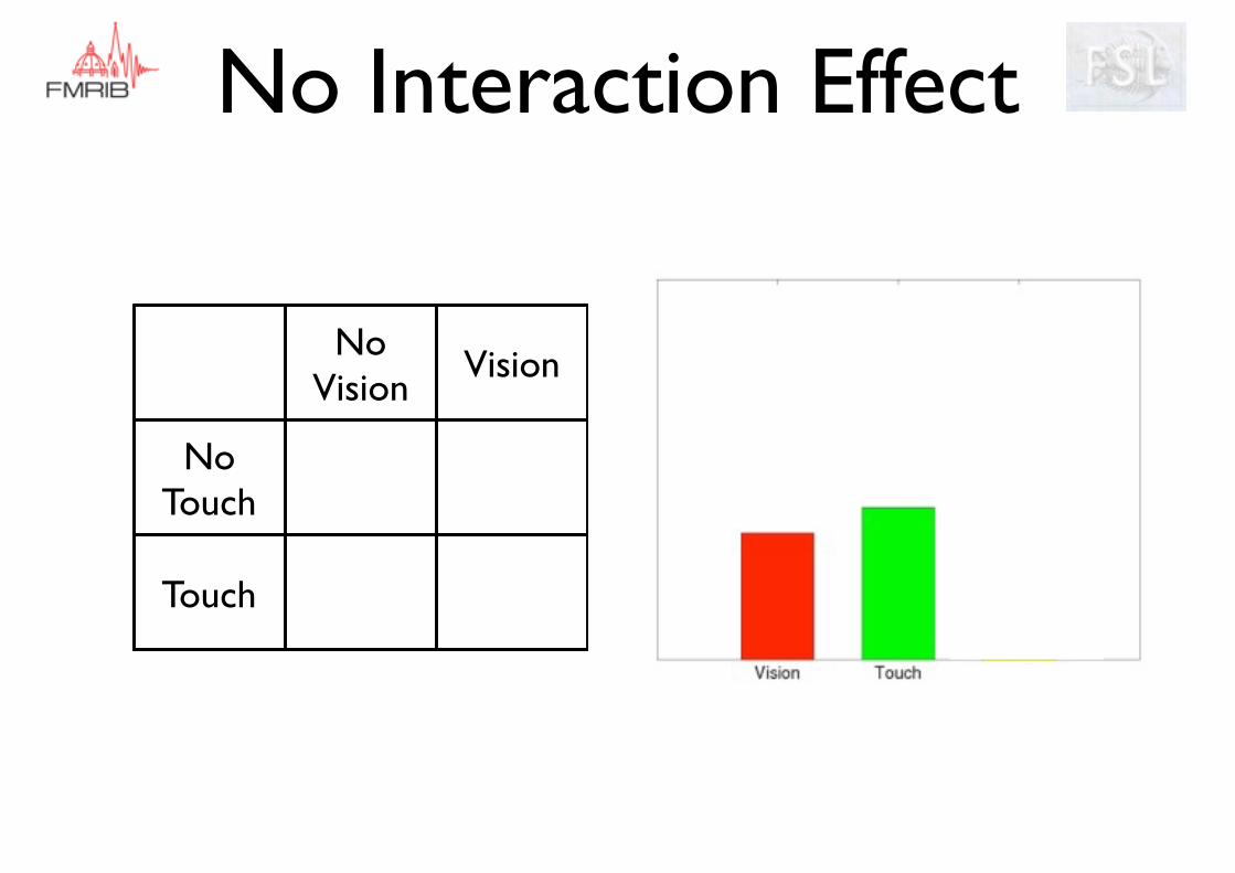
No Interaction Effect
No Vision
Vision
No Touch
Touch
No Interaction Effect
No Vision
Vision
No Touch
Touch
No Interaction Effect
No Vision
Vision
No Touch
Touch
No interaction - effects add linearly
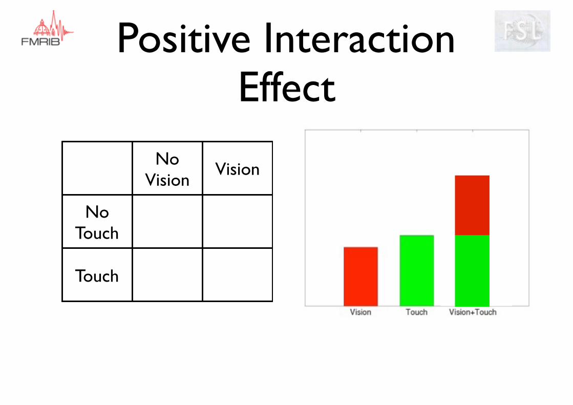
Positive Interaction Effect
No Vision
Vision
No Touch
Touch
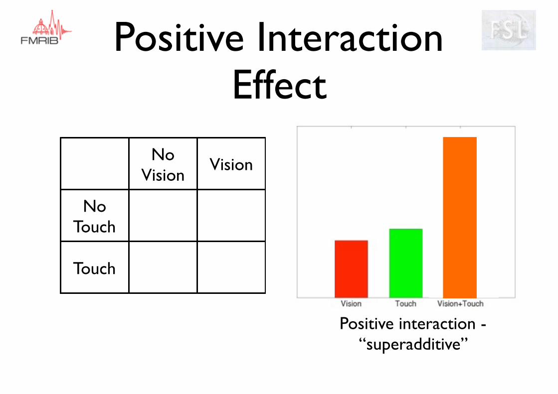
Positive Interaction Effect
No Vision
Vision
No Touch
Touch
Positive interaction - “superadditive”
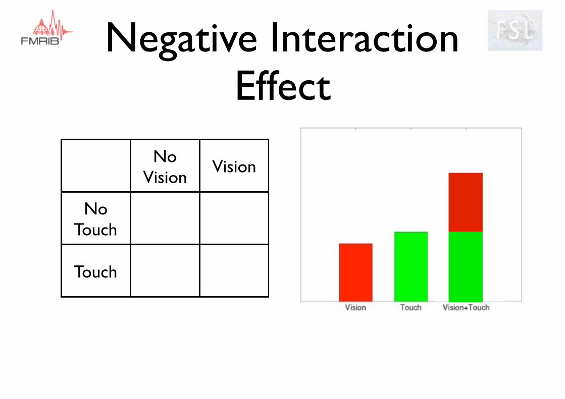
Negative Interaction Effect
No Vision
Vision
No Touch
Touch
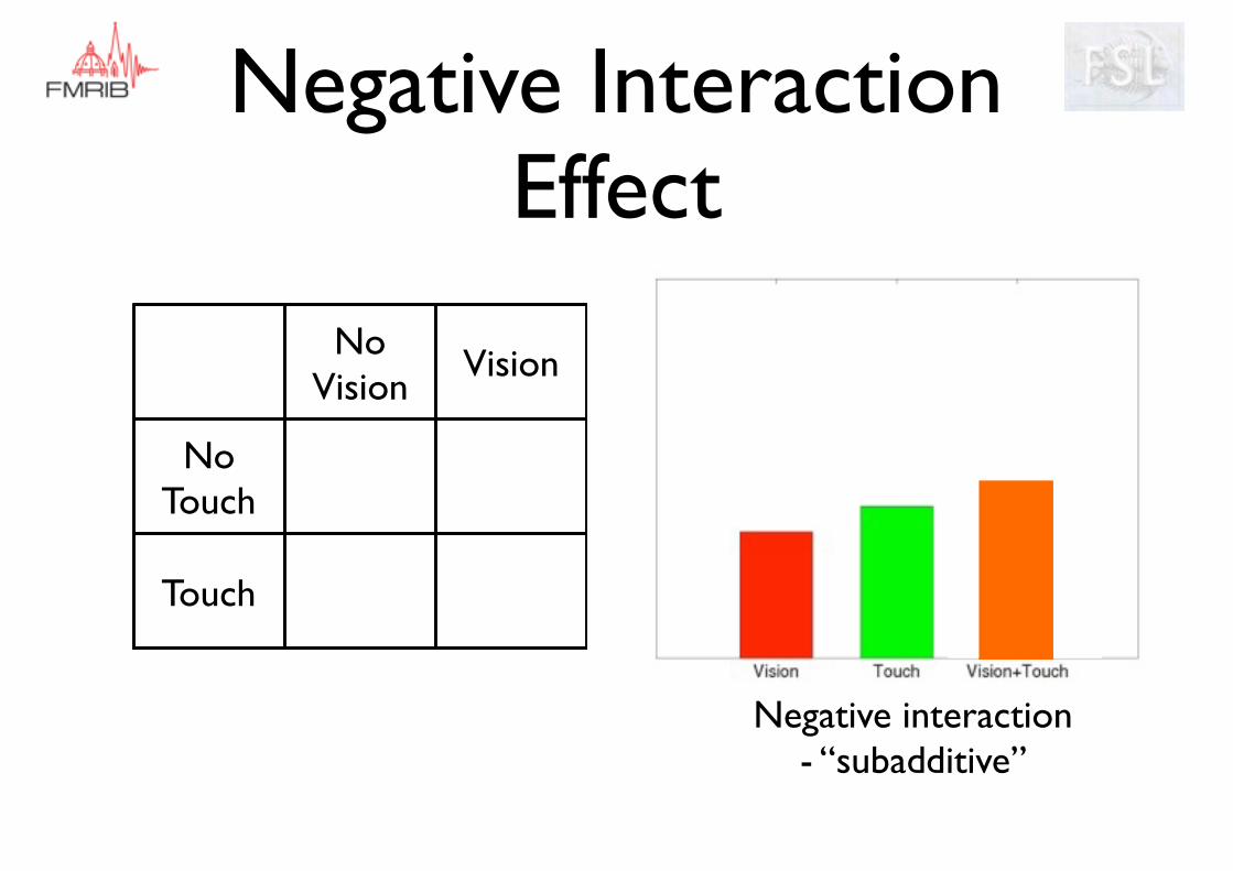
Negative Interaction Effect
No Vision
Vision
No Touch
Touch
Negative interaction - “subadditive”
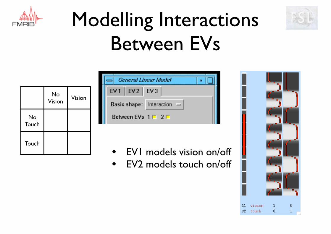
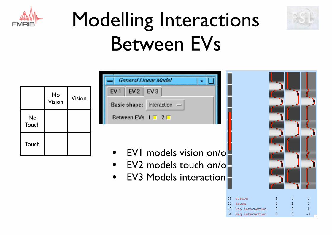
Modelling Interactions Between EVs
• EV1 models vision on/off• EV2 models touch on/off
No Vision
Vision
No Touch
Touch
Modelling Interactions Between EVs
• EV1 models vision on/off• EV2 models touch on/off• EV3 Models interaction
No Vision
Vision
No Touch
Touch
Correlation of EVs
• Correlated EVs are relatively common, but strong correlation is a problem in either first-level or group-level designs.
• When EVs are correlated, it is the unique contribution from each EV that determines the model’s fit to the data and the statistics.
• Start by looking at first-level examples:• correlation and rank deficiency• design efficiency tool
Correlation of EVs
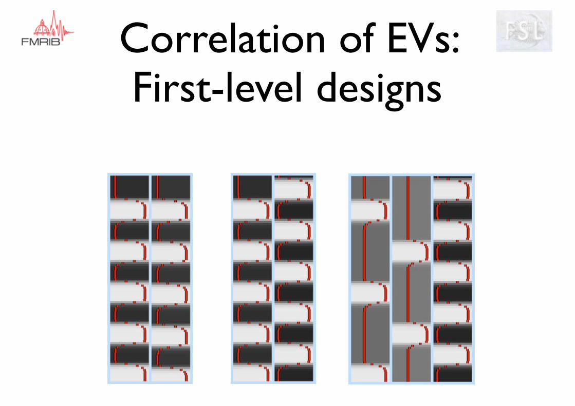
Correlation of EVs: First-level designs
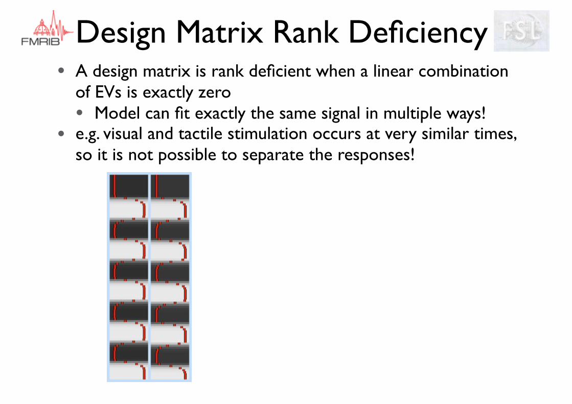
Design Matrix Rank Deficiency• A design matrix is rank deficient when a linear combination
of EVs is exactly zero• Model can fit exactly the same signal in multiple ways!
• e.g. visual and tactile stimulation occurs at very similar times, so it is not possible to separate the responses!
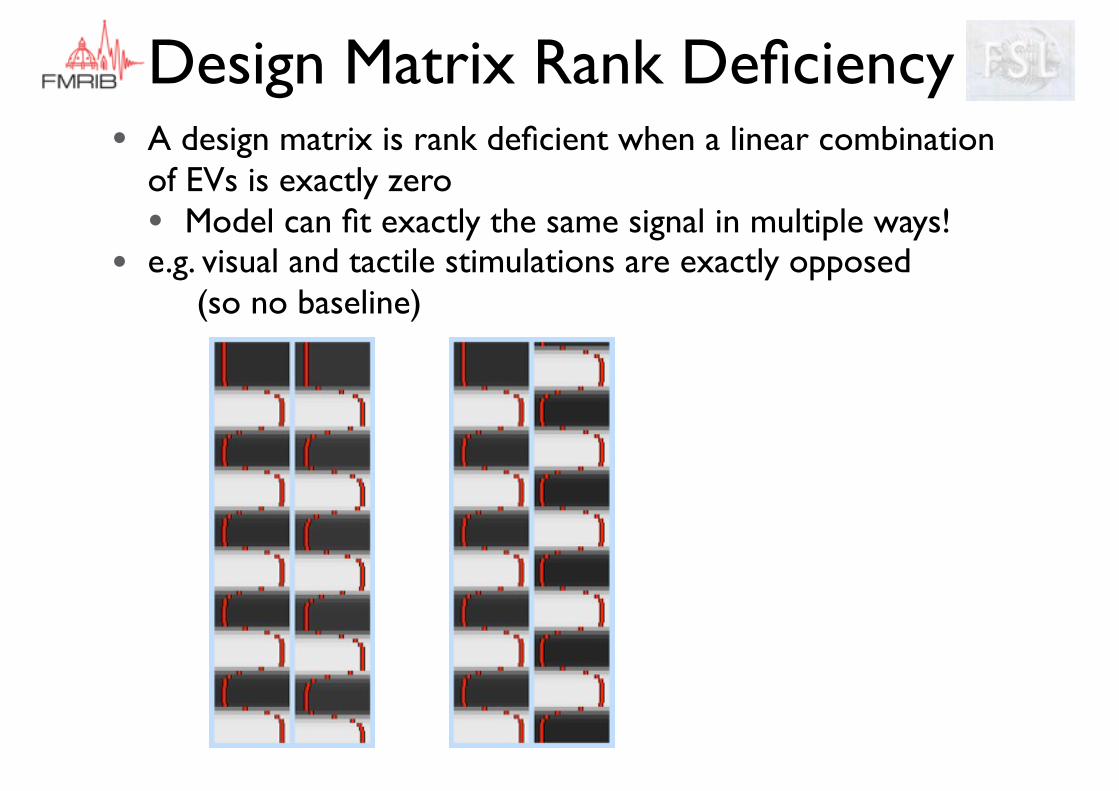
Design Matrix Rank Deficiency• A design matrix is rank deficient when a linear combination
of EVs is exactly zero• Model can fit exactly the same signal in multiple ways!
• e.g. visual and tactile stimulations are exactly opposed (so no baseline)
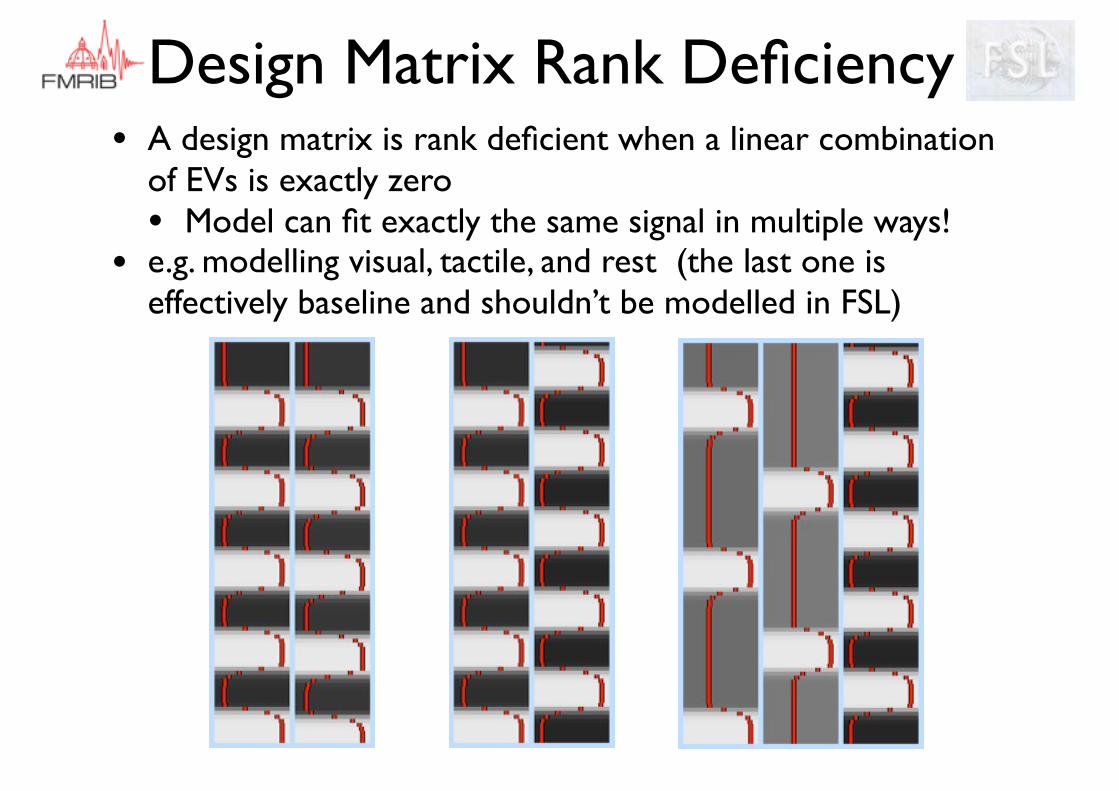
Design Matrix Rank Deficiency• A design matrix is rank deficient when a linear combination
of EVs is exactly zero• Model can fit exactly the same signal in multiple ways!
• e.g. modelling visual, tactile, and rest (the last one is effectively baseline and shouldn’t be modelled in FSL)

• Good News: The statistics always take care of being close to rank deficient
Close to Rank Deficient Design Matrices
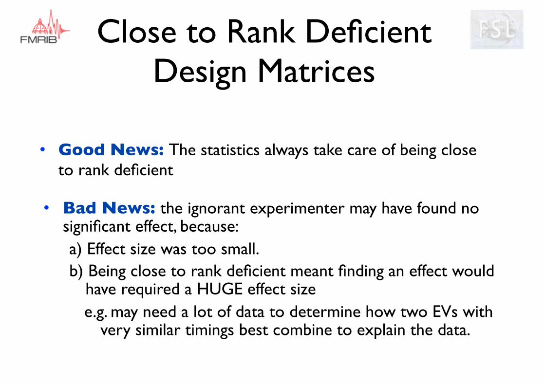
• Good News: The statistics always take care of being close to rank deficient
• Bad News: the ignorant experimenter may have found no significant effect, because:a) Effect size was too small.b) Being close to rank deficient meant finding an effect would
have required a HUGE effect sizee.g. may need a lot of data to determine how two EVs with
very similar timings best combine to explain the data.
Close to Rank Deficient Design Matrices

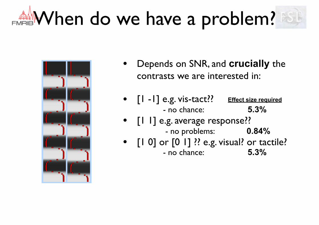
When do we have a problem?
• Depends on SNR, and crucially the contrasts we are interested in:
• [1 -1] e.g. vis-tact??
• [1 1] e.g. average response??
• [1 0] or [0 1] ?? e.g. visual? or tactile?
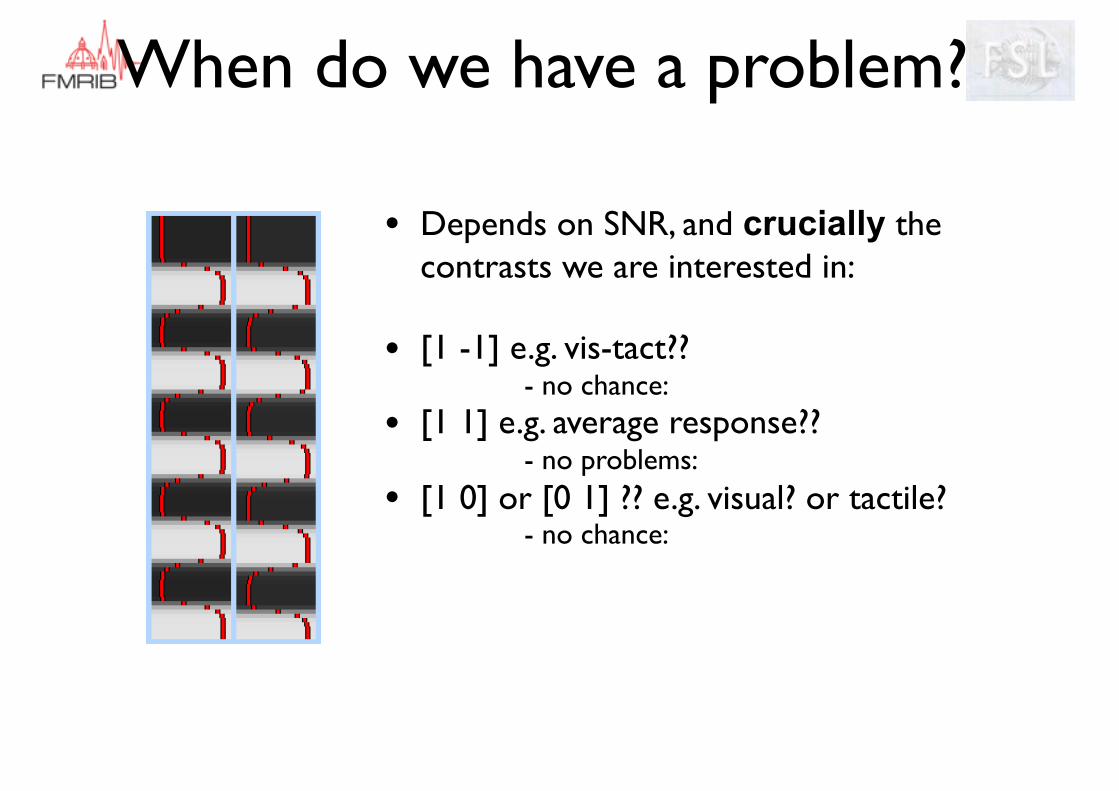
When do we have a problem?
• Depends on SNR, and crucially the contrasts we are interested in:
• [1 -1] e.g. vis-tact?? - no chance:
• [1 1] e.g. average response?? - no problems:
• [1 0] or [0 1] ?? e.g. visual? or tactile? - no chance:
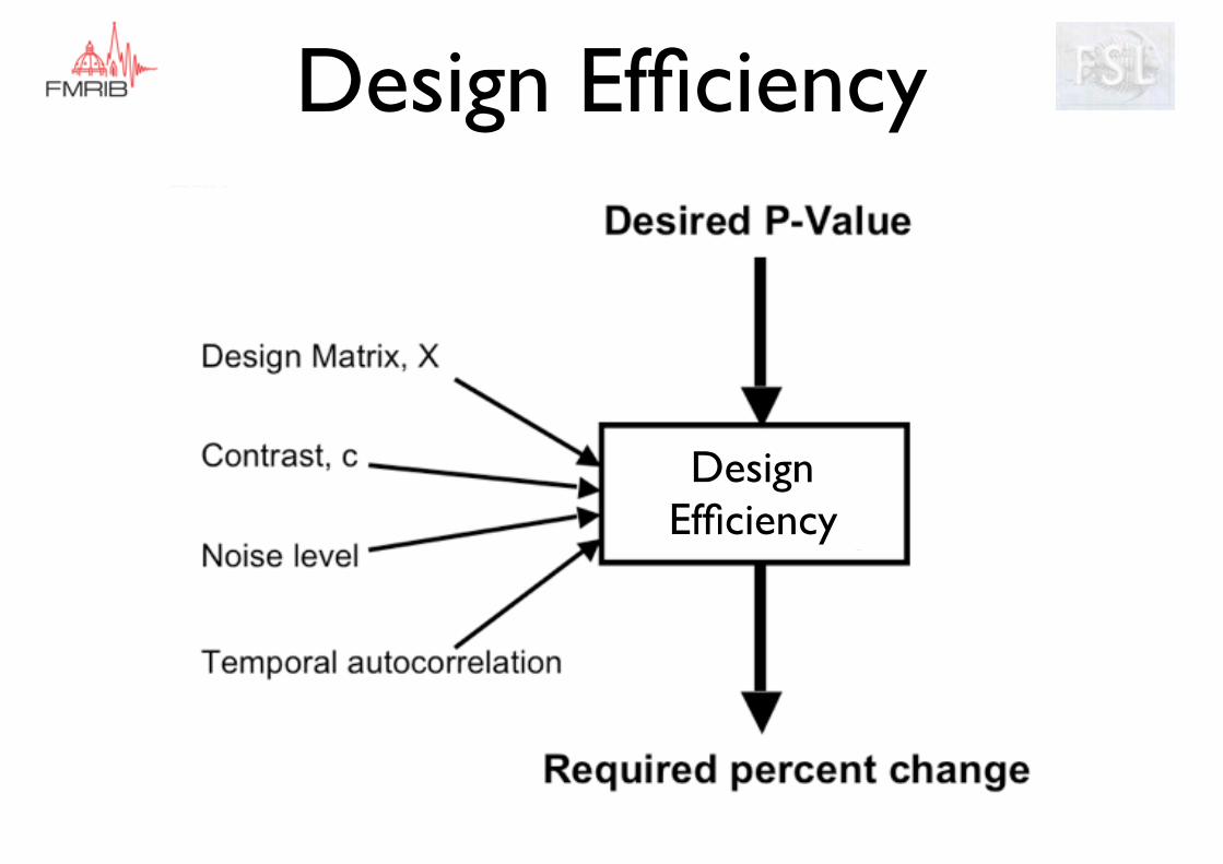
Design Efficiency
Design Efficiency
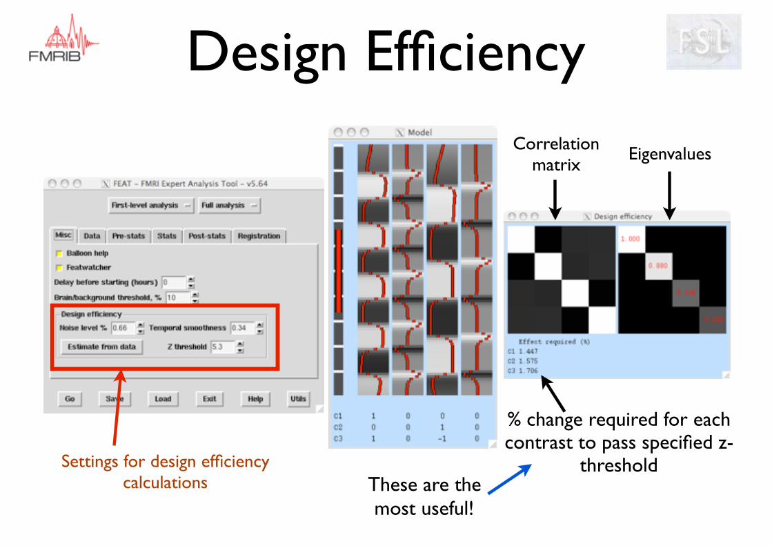
Design Efficiency
% change required for each contrast to pass specified z-
threshold
Correlation matrix
Eigenvalues
Settings for design efficiency calculations These are the
most useful!
When do we have a problem?
• Depends on SNR, and crucially the contrasts we are interested in:
• [1 -1] e.g. vis-tact??- no chance: 5.3%
• [1 1] e.g. average response?? - no problems: 0.84%
• [1 0] or [0 1] ?? e.g. visual? or tactile?- no chance: 5.3%
Effect size required
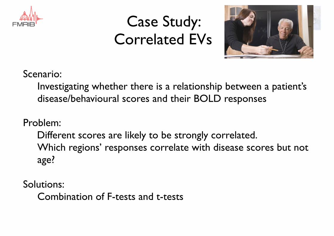
Case Study: Correlated EVs
Scenario: Investigating whether there is a relationship between a patient’s disease/behavioural scores and their BOLD responses
Problem: Different scores are likely to be strongly correlated.Which regions’ responses correlate with disease scores but not age?
Solutions:Combination of F-tests and t-tests
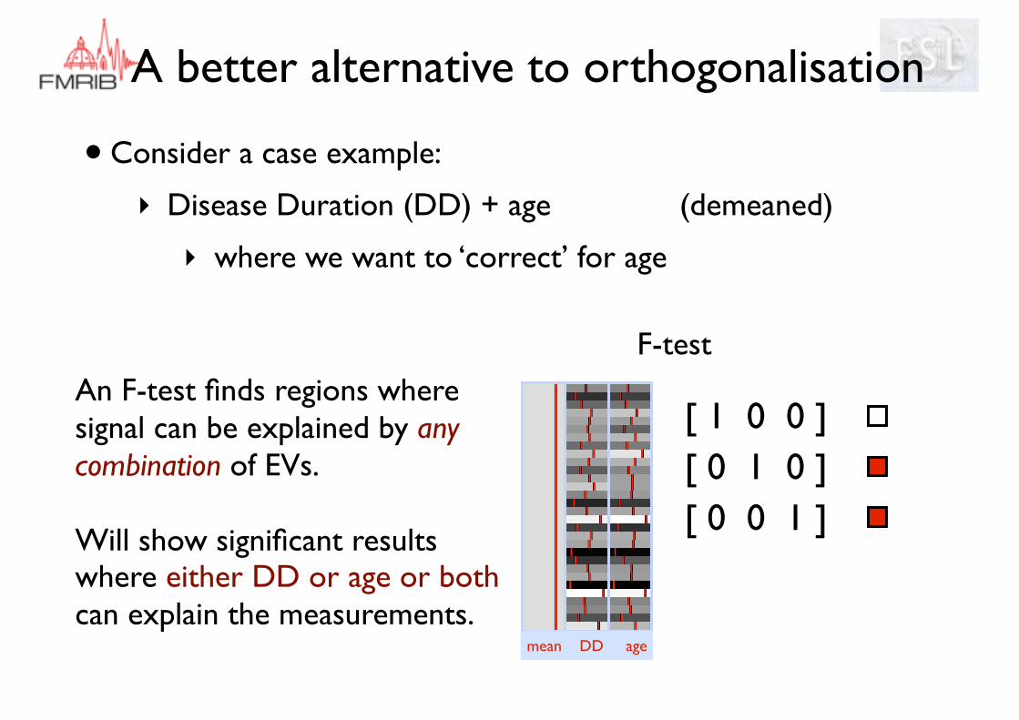
• Consider a case example:
‣ Disease Duration (DD) + age
‣ where we want to ‘correct’ for age
(demeaned)
Correlations, Covariates & Corrections
Correlations, Covariates & Corrections
• Consider a case example:
‣ Disease Duration (DD) + age
‣ where we want to ‘correct’ for age
‣ If there is correlation between DD and age then it becomes tricky
‣ One option is orthogonalisation of DD and age …
(demeaned)
A better alternative to orthogonalisation
• Consider a case example:
‣ Disease Duration (DD) + age
‣ where we want to ‘correct’ for age
(demeaned)
A better alternative to orthogonalisation
mean DoD ag
[ 0 1 0 ]
t-test
mean DD age
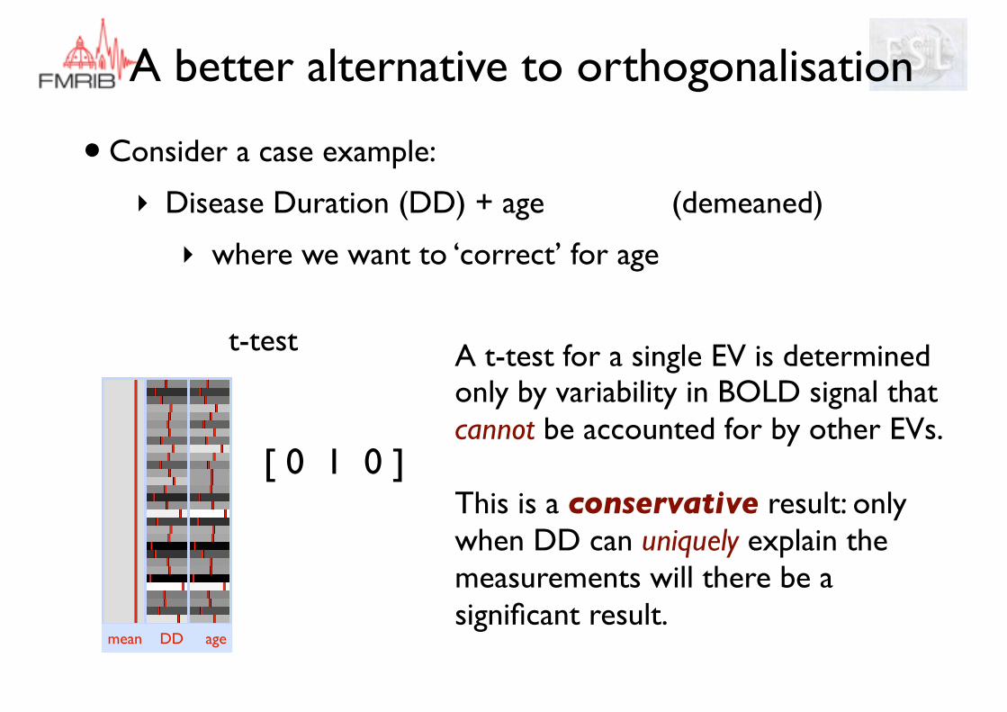
• Consider a case example:
‣ Disease Duration (DD) + age
‣ where we want to ‘correct’ for age
A t-test for a single EV is determined only by variability in BOLD signal that cannot be accounted for by other EVs.
This is a conservative result: only when DD can uniquely explain the measurements will there be a significant result.
(demeaned)
A better alternative to orthogonalisation
mean DoD ag
[ 0 1 0 ]
t-test
mean DoD ag
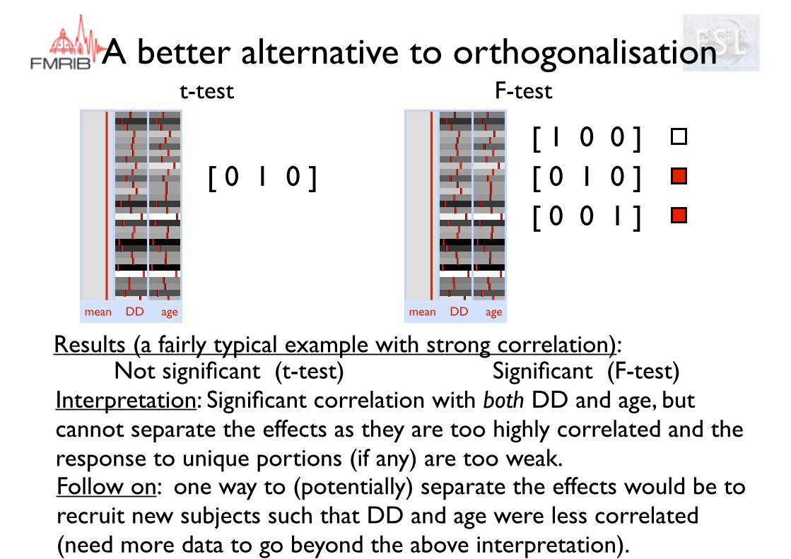
[ 0 0 1 ][ 0 1 0 ][ 1 0 0 ]
F-test
mean DD age mean DD age
• Consider a case example:
‣ Disease Duration (DD) + age
‣ where we want to ‘correct’ for age
(demeaned)
A better alternative to orthogonalisation
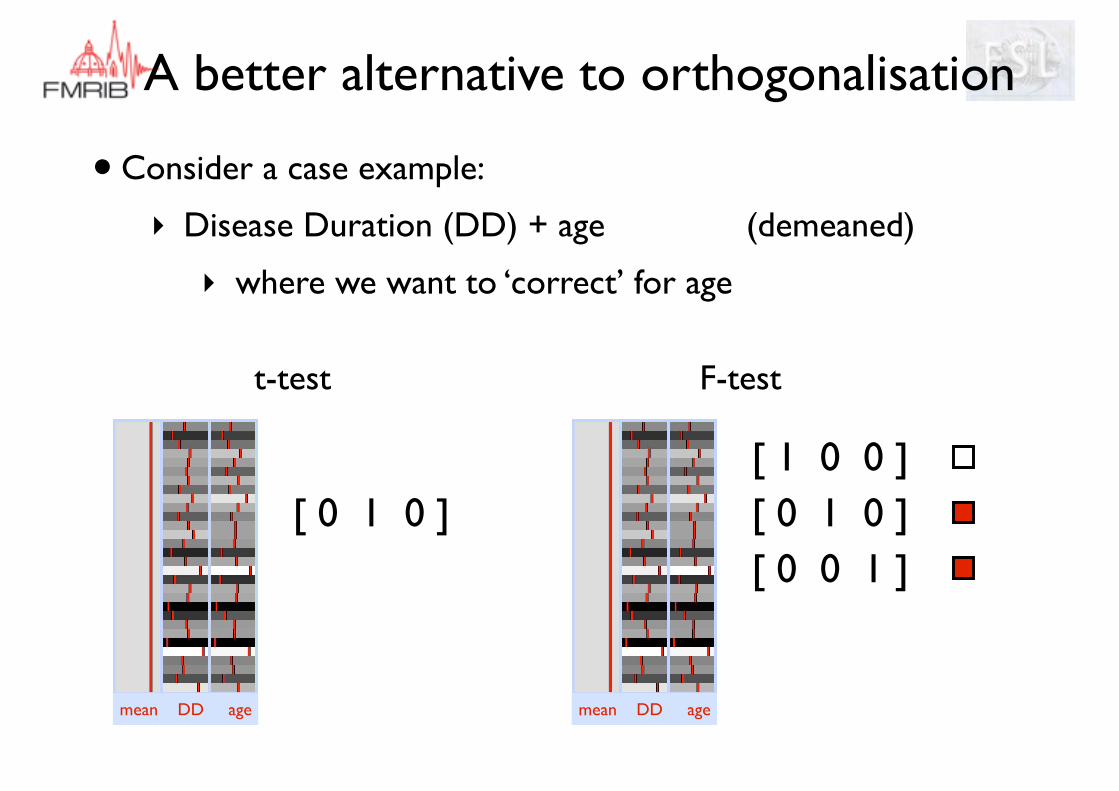
mean DoD ag
[ 0 0 1 ][ 0 1 0 ][ 1 0 0 ]
F-test
mean DD age
• Consider a case example:
‣ Disease Duration (DD) + age
‣ where we want to ‘correct’ for age
(demeaned)
An F-test finds regions where signal can be explained by any combination of EVs.
Will show significant results where either DD or age or both can explain the measurements.
A better alternative to orthogonalisation
mean DoD ag
[ 0 1 0 ]
t-test
mean DoD ag
[ 0 0 1 ][ 0 1 0 ][ 1 0 0 ]
F-test
Not significant (t-test)Results (a fairly typical example with strong correlation):
Interpretation: Significant correlation with both DD and age, but cannot separate the effects as they are too highly correlated and the response to unique portions (if any) are too weak.
Significant (F-test)
Follow on: one way to (potentially) separate the effects would be to recruit new subjects such that DD and age were less correlated (need more data to go beyond the above interpretation).
mean DD age mean DD age

That’s All Folks
Appendix
Case Studies:
• HRF Variability
• Perfusion FMRI
• Orthogonalisation & more on demeaning
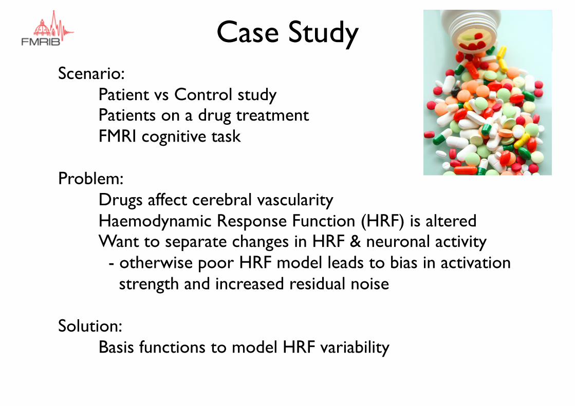
Case StudyScenario:
Patient vs Control studyPatients on a drug treatmentFMRI cognitive task
Problem:Drugs affect cerebral vascularityHaemodynamic Response Function (HRF) is alteredWant to separate changes in HRF & neuronal activity - otherwise poor HRF model leads to bias in activation
strength and increased residual noise
Solution:Basis functions to model HRF variability
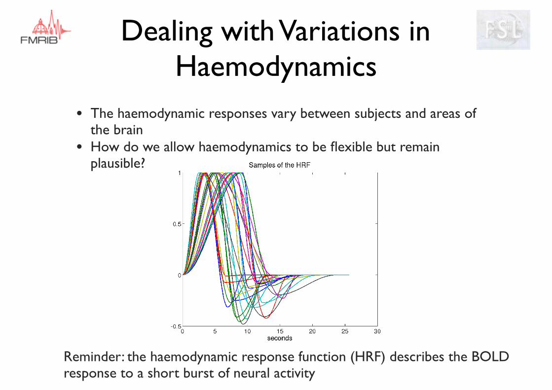
Dealing with Variations in Haemodynamics
• The haemodynamic responses vary between subjects and areas of the brain
• How do we allow haemodynamics to be flexible but remain plausible?
Reminder: the haemodynamic response function (HRF) describes the BOLD response to a short burst of neural activity
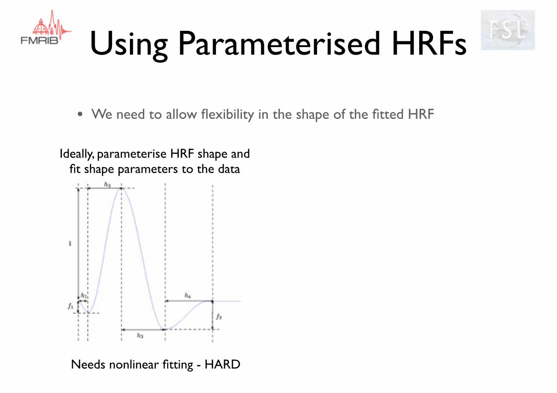
• We need to allow flexibility in the shape of the fitted HRF
Ideally, parameterise HRF shape and fit shape parameters to the data
Needs nonlinear fitting - HARD
Using Parameterised HRFs
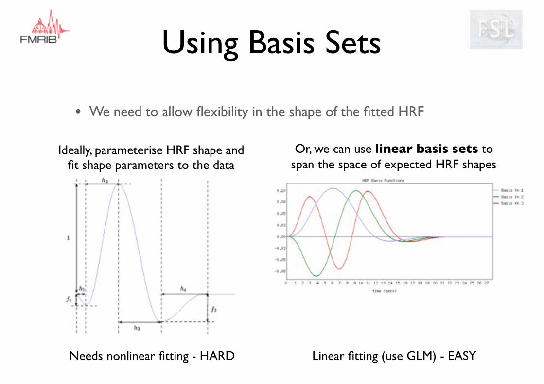
Using Basis Sets
• We need to allow flexibility in the shape of the fitted HRF
Or, we can use linear basis sets to span the space of expected HRF shapes
Needs nonlinear fitting - HARD Linear fitting (use GLM) - EASY
Ideally, parameterise HRF shape and fit shape parameters to the data
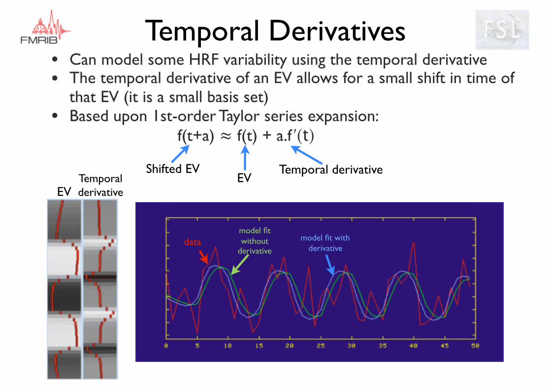
Temporal Derivatives• Can model some HRF variability using the temporal derivative• The temporal derivative of an EV allows for a small shift in time of
that EV (it is a small basis set)• Based upon 1st-order Taylor series expansion:
f(t+a) ≈ f(t) + a.f ʹ(t)
EVTemporal derivative
datamodel fit without
derivative
model fit with derivative
EVShifted EV Temporal derivative
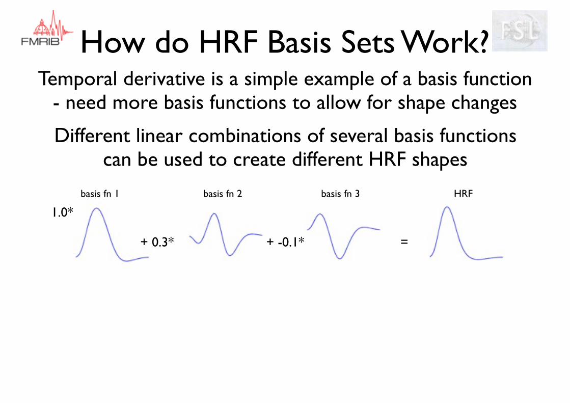
How do HRF Basis Sets Work?
Different linear combinations of several basis functions can be used to create different HRF shapes
+ -0.1*+ 0.3*
1.0*
=
basis fn 1 basis fn 2 basis fn 3 HRF
Temporal derivative is a simple example of a basis function- need more basis functions to allow for shape changes
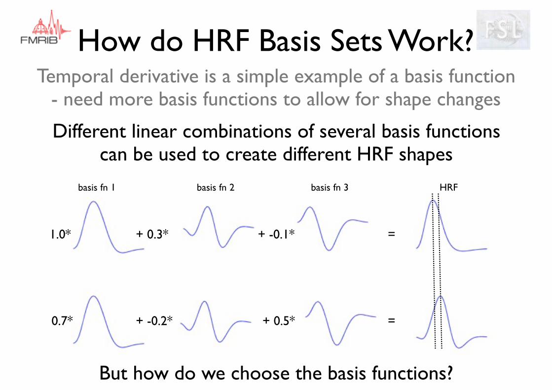
How do HRF Basis Sets Work?
+ -0.1*+ 0.3* 1.0* =
+ 0.5*+ -0.2* 0.7* =
basis fn 1 basis fn 2 basis fn 3 HRF
But how do we choose the basis functions?
Different linear combinations of several basis functions can be used to create different HRF shapes
Temporal derivative is a simple example of a basis function- need more basis functions to allow for shape changes
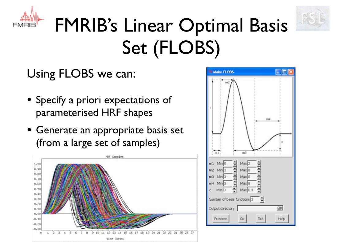
FMRIB’s Linear Optimal Basis Set (FLOBS)
Using FLOBS we can:
• Specify a priori expectations of parameterised HRF shapes
• Generate an appropriate basis set (from a large set of samples)

Select the main modes of variation as the optimal basis set
“Canonical HRF”dispersion derivative temporal
derivative
FMRIB’s Linear Optimal Basis Set (FLOBS)
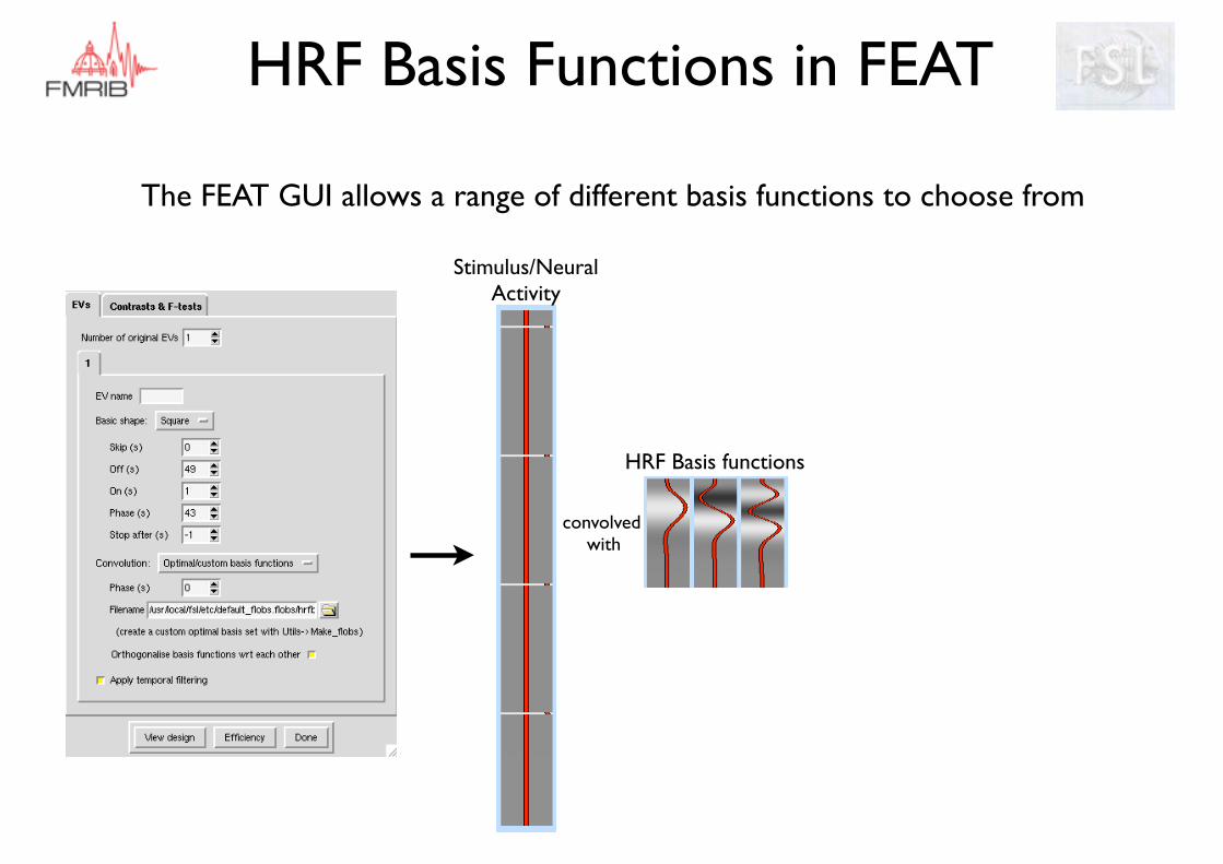
HRF Basis Functions in FEAT
The FEAT GUI allows a range of different basis functions to choose from
HRF Basis functions
Stimulus/Neural Activity
convolved with
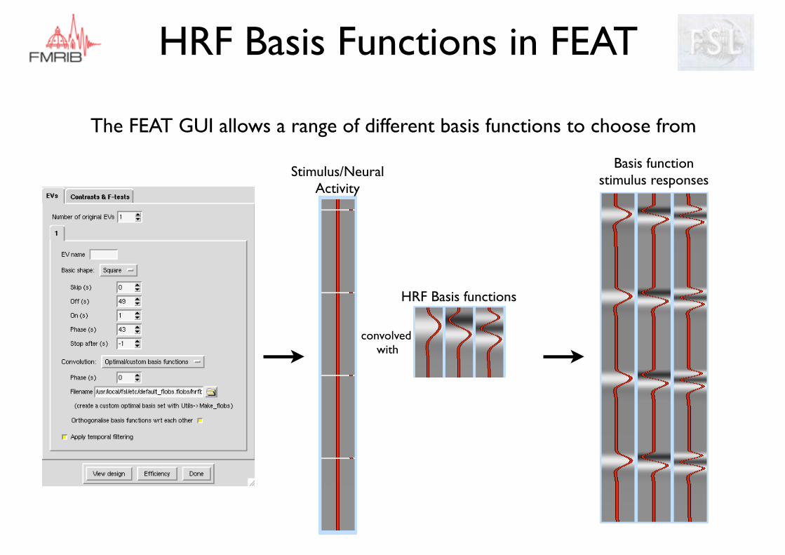
HRF Basis Functions in FEAT
The FEAT GUI allows a range of different basis functions to choose from
HRF Basis functions
Stimulus/Neural Activity
convolved with
Basis function stimulus responses
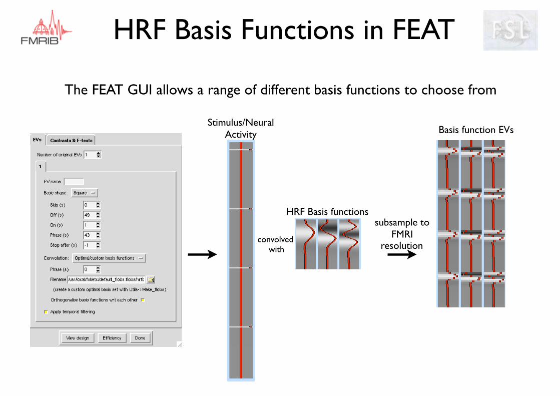
HRF Basis Functions in FEAT
The FEAT GUI allows a range of different basis functions to choose from
HRF Basis functions
Stimulus/Neural Activity
convolved with
Basis function EVs
subsample to FMRI
resolution
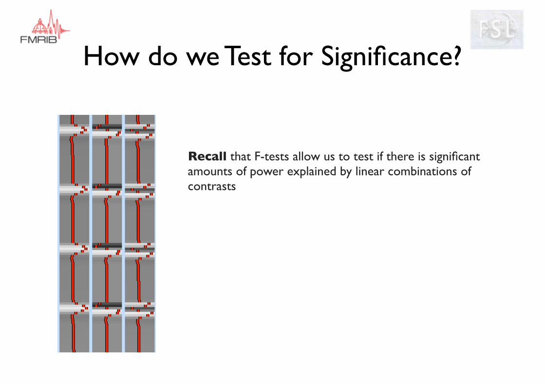
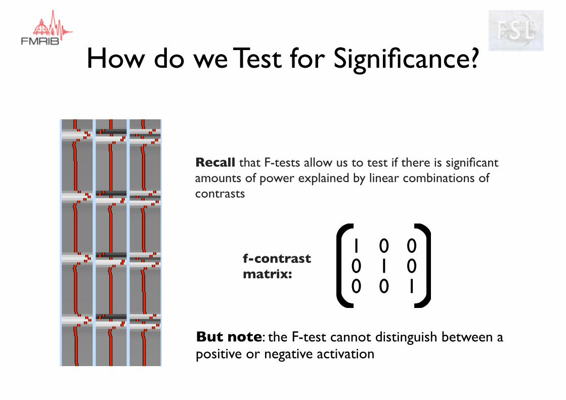
How do we Test for Significance?
Recall that F-tests allow us to test if there is significant amounts of power explained by linear combinations of contrasts
How do we Test for Significance?
Recall that F-tests allow us to test if there is significant amounts of power explained by linear combinations of contrasts
1 0 0
0 0 10 1 0f-contrast
matrix:
But note: the F-test cannot distinguish between a positive or negative activation
HRF Basis Functions in FEAT
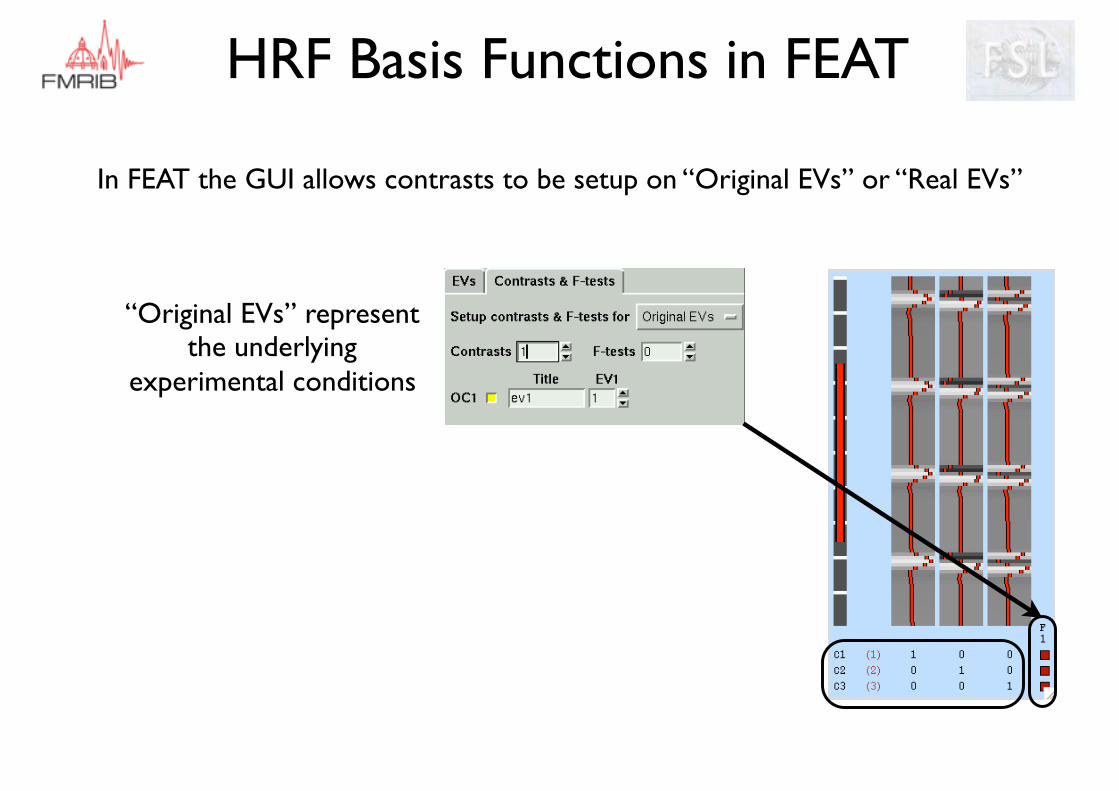
In FEAT the GUI allows contrasts to be setup on “Original EVs” or “Real EVs”
“Original EVs” represent the underlying
experimental conditions
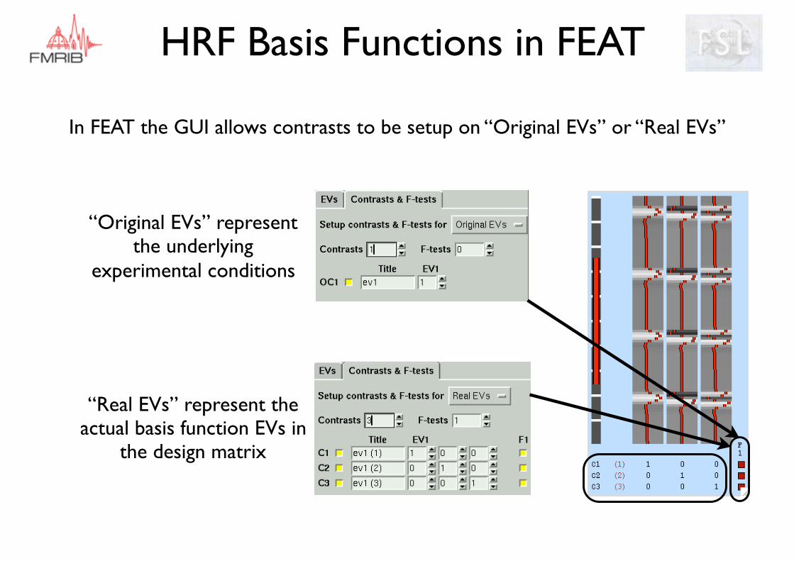
HRF Basis Functions in FEAT
In FEAT the GUI allows contrasts to be setup on “Original EVs” or “Real EVs”
“Original EVs” represent the underlying
experimental conditions
“Real EVs” represent the actual basis function EVs in
the design matrix
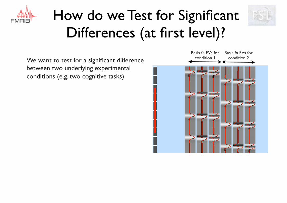
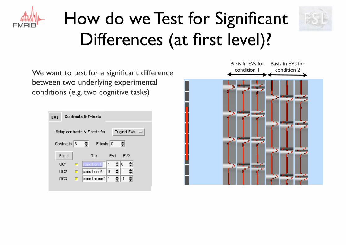
How do we Test for Significant Differences (at first level)?
We want to test for a significant difference between two underlying experimental conditions (e.g. two cognitive tasks)
Basis fn EVs for condition 1
Basis fn EVs for condition 2
We want to test for a significant difference between two underlying experimental conditions (e.g. two cognitive tasks)
Basis fn EVs for condition 1
Basis fn EVs for condition 2
How do we Test for Significant Differences (at first level)?
Basis fn EVs for condition 1
Basis fn EVs for condition 2
How do we Test for Significant Differences (at first level)?
We want to test for a significant difference between two underlying experimental conditions (e.g. two cognitive tasks)
Basis fn EVs for condition 1
Basis fn EVs for condition 2
How do we Test for Significant Differences (at first level)?
We want to test for a significant difference between two underlying experimental conditions (e.g. two cognitive tasks)
Basis fn EVs for condition 1
Basis fn EVs for condition 2
How do we Test for Significant Differences (at first level)?
We want to test for a significant difference between two underlying experimental conditions (e.g. two cognitive tasks)
Basis fn EVs for condition 1
Basis fn EVs for condition 2
• F-test combines [1 -1] t-contrasts for corresponding basis fn EVs
• this will find significance if there are size or shape differences
How do we Test for Significant Differences (at first level)?
We want to test for a significant difference between two underlying experimental conditions (e.g. two cognitive tasks)
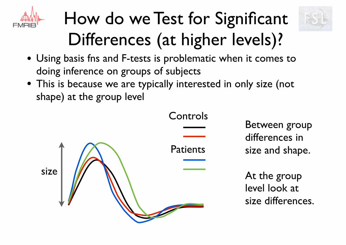
• Using basis fns and F-tests is problematic when it comes to doing inference on groups of subjects
• This is because we are typically interested in only size (not shape) at the group level
How do we Test for Significant Differences (at higher levels)?
Controls
Patients
Between group differences in size and shape.
At the group level look at size differences.
size
• Using basis fns and F-tests is problematic when it comes to doing inference on groups of subjects
• This is because we are typically interested in only size (not shape) at the group level
• Options:
1) Only use the “canonical HRF” EV PE in the group inference - e.g. when EVs with temporal derivatives, only use the main EV’s PE in the group inference
How do we Test for Significant Differences (at higher levels)?
• Using basis fns and F-tests is problematic when it comes to doing inference on groups of subjects
• This is because we are typically interested in only size (not shape) at the group level
2) Calculate a “size” statistic from the basis function EVs PEs and use in the group inference - must use randomise for this, not standard FEAT/FLAME
• Options:
1) Only use the “canonical HRF” EV PE in the group inference - e.g. when EVs with temporal derivatives, only use the main EV’s PE in the group inference
How do we Test for Significant Differences (at higher levels)?
Case Study
Scenario:Pain study of tonic, ongoing pain and involving infusion of drugs during scanning(or any other slow-acting physiological stimuli e.g. thirst)
Problem:Very slow changes in BOLD activity (> several minutes) - slow drifts in noise cannot be separated from neuronally-induced BOLD activity by normal temporal filtering
Solution:Alternative to BOLD = Arterial Spin Labelling (ASL)
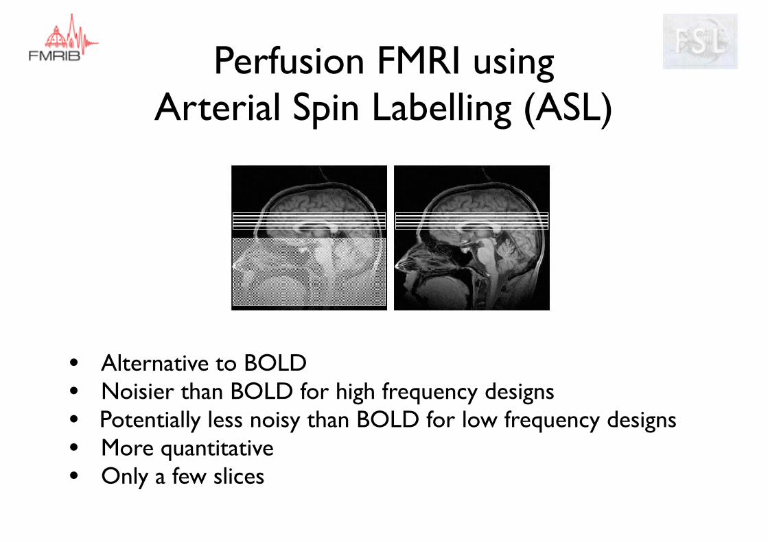
Perfusion FMRI using Arterial Spin Labelling (ASL)
• Alternative to BOLD• Noisier than BOLD for high frequency designs• Potentially less noisy than BOLD for low frequency designs• More quantitative• Only a few slices
Tag Control
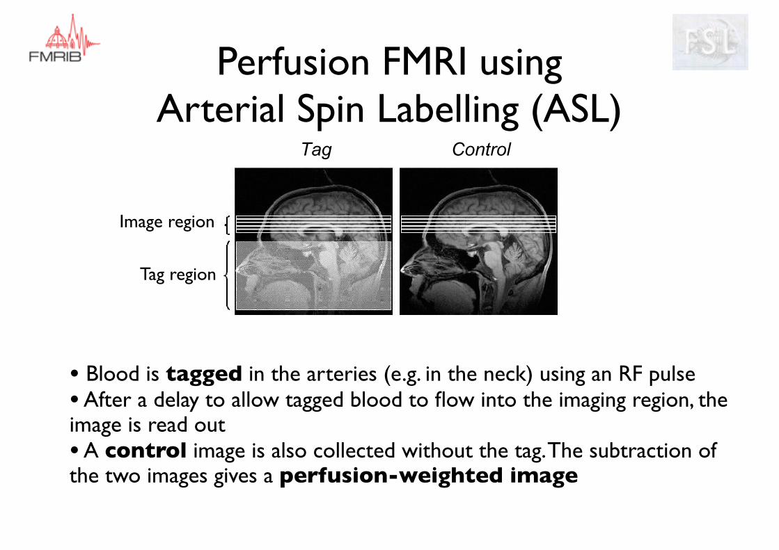
Perfusion FMRI using Arterial Spin Labelling (ASL)
• Blood is tagged in the arteries (e.g. in the neck) using an RF pulse• After a delay to allow tagged blood to flow into the imaging region, the image is read out• A control image is also collected without the tag. The subtraction of the two images gives a perfusion-weighted image
Tag Control
Tag region
Image region
Perfusion FMRI Modelling
•Timeseries alternates between "control" (up) and "tag" (down)•Activation seen as modulation of control-tag difference •There are two GLM approaches available in FEAT:

Perfusion FMRI Modelling
•Timeseries alternates between "control" (up) and "tag" (down)•Activation seen as modulation of control-tag difference •There are two GLM approaches available in FEAT:
1) Pre-subtract data (using sinc interpolation)
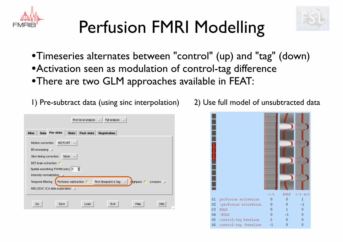
Perfusion FMRI Modelling
•Timeseries alternates between "control" (up) and "tag" (down)•Activation seen as modulation of control-tag difference •There are two GLM approaches available in FEAT:
1) Pre-subtract data (using sinc interpolation) 2) Use full model of unsubtracted data
Simultaneous BOLD and Perfusion FMRI Modelling
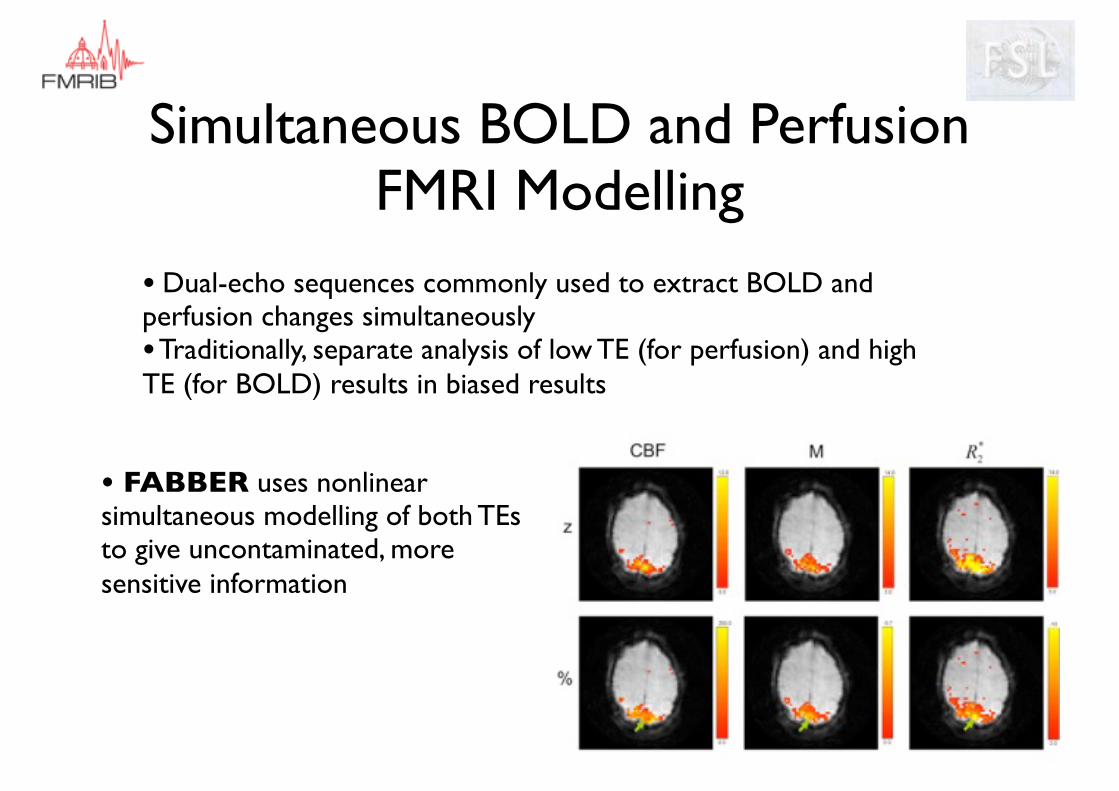
• Dual-echo sequences commonly used to extract BOLD and perfusion changes simultaneously• Traditionally, separate analysis of low TE (for perfusion) and high TE (for BOLD) results in biased results
• Dual-echo sequences commonly used to extract BOLD and perfusion changes simultaneously• Traditionally, separate analysis of low TE (for perfusion) and high TE (for BOLD) results in biased results
• FABBER uses nonlinear simultaneous modelling of both TEs to give uncontaminated, more sensitive information
Simultaneous BOLD and Perfusion FMRI Modelling
Orthogonalisation - A cautionary tale
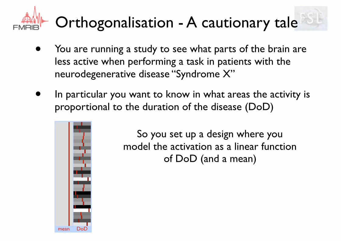
• You are running a study to see what parts of the brain are less active when performing a task in patients with the neurodegenerative disease “Syndrome X”
• In particular you want to know in what areas the activity is proportional to the duration of the disease (DoD)
mean DoD
So you set up a design where you model the activation as a linear function
of DoD (and a mean)
Orthogonalisation - A cautionary tale
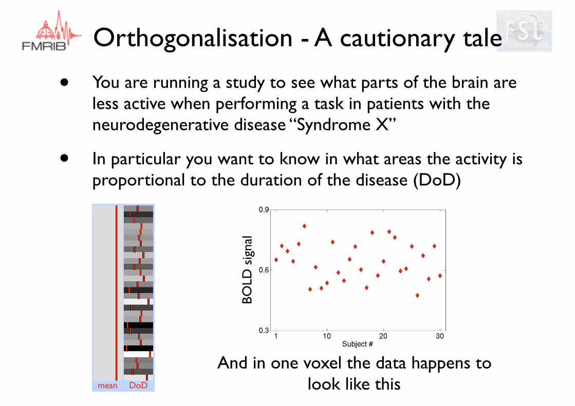
• You are running a study to see what parts of the brain are less active when performing a task in patients with the neurodegenerative disease “Syndrome X”
• In particular you want to know in what areas the activity is proportional to the duration of the disease (DoD)
mean DoD
And in one voxel the data happens to look like this
BOLD
sig
nal
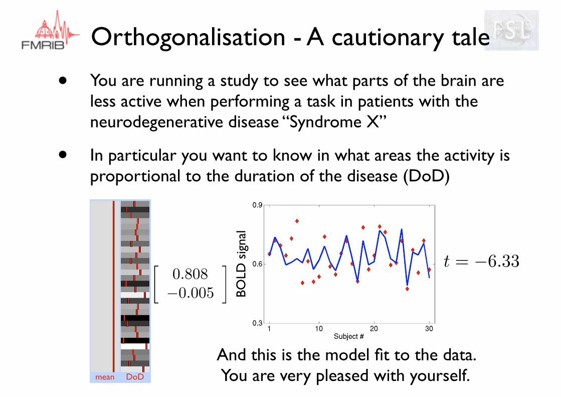
Orthogonalisation - A cautionary tale
• You are running a study to see what parts of the brain are less active when performing a task in patients with the neurodegenerative disease “Syndrome X”
• In particular you want to know in what areas the activity is proportional to the duration of the disease (DoD)
mean DoD
And this is the model fit to the data. You are very pleased with yourself.
�0.808�0.005
� t = �6.33BO
LD s
igna
l
Orthogonalisation - A cautionary tale
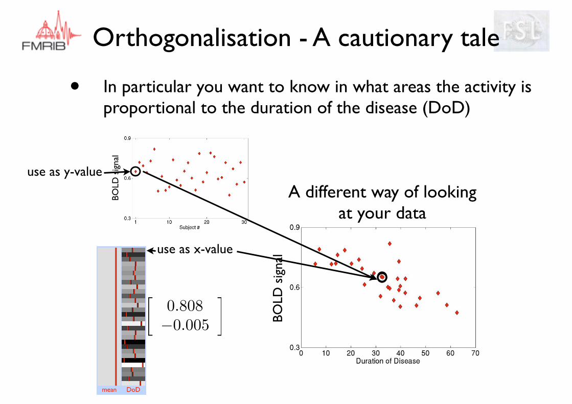
• In particular you want to know in what areas the activity is proportional to the duration of the disease (DoD)
mean DoD
�0.808�0.005
�
use as x-value
use as y-value
A different way of looking at your data
BOLD
sig
nal
BO
LD s
igna
l
Orthogonalisation - A cautionary tale
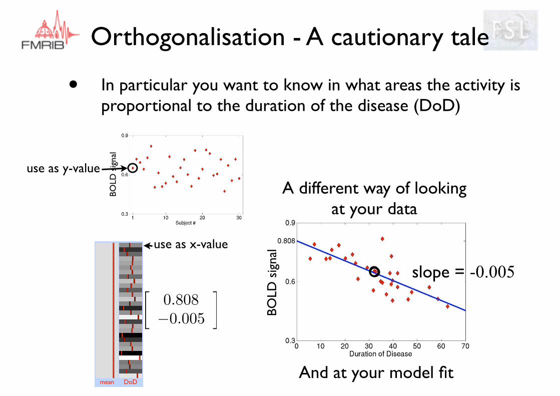
• In particular you want to know in what areas the activity is proportional to the duration of the disease (DoD)
mean DoD
�0.808�0.005
�
use as x-value
use as y-value
A different way of looking at your data
And at your model fit
slope = -0.005BO
LD s
igna
l
BO
LD s
igna
l
Orthogonalisation - A cautionary tale
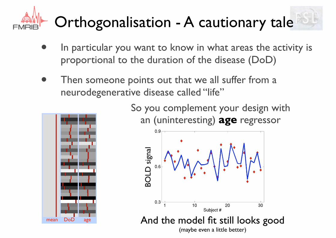
• In particular you want to know in what areas the activity is proportional to the duration of the disease (DoD)
• Then someone points out that we all suffer from a neurodegenerative disease called “life”
mean DoD age
So you complement your design with an (uninteresting) age regressor
And the model fit still looks good (maybe even a little better)
BOLD
sig
nal

Orthogonalisation - A cautionary tale
• In particular you want to know in what areas the activity is proportional to the duration of the disease (DoD)
• Then someone points out that we all suffer from a neurodegenerative disease called “life”
mean DoD age
And you test your DoD for significance
What on earth just happened?
[ 0 1 0 ]
t = 0.11BO
LD s
igna
l
Orthogonalisation - A cautionary tale
• In particular you want to know in what areas the activity is proportional to the duration of the disease (DoD)
• Then someone points out that we all suffer from a neurodegenerative disease called “life”
mean DoD age
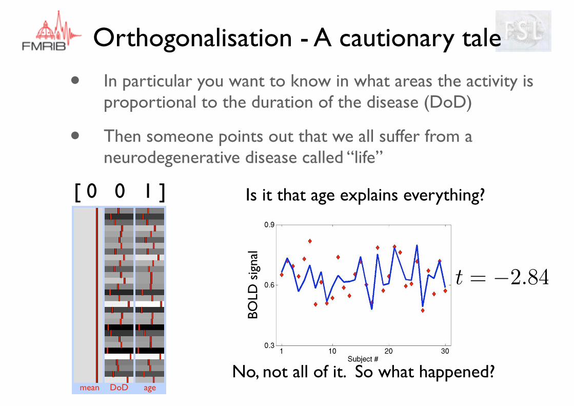
Is it that age explains everything?
No, not all of it. So what happened?
[ 0 0 1 ]
t = �2.84BO
LD s
igna
l
Orthogonalisation - A cautionary tale
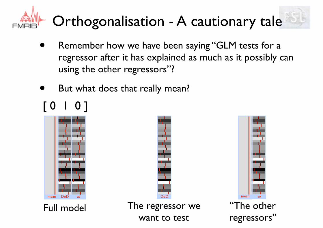
• Remember how we have been saying “GLM tests for a regressor after it has explained as much as it possibly can using the other regressors”?
• But what does that really mean?
mean DoD ag
[ 0 1 0 ]
Full modelDoD
The regressor we want to test
mean ag
“The other regressors”
Orthogonalisation - A cautionary tale
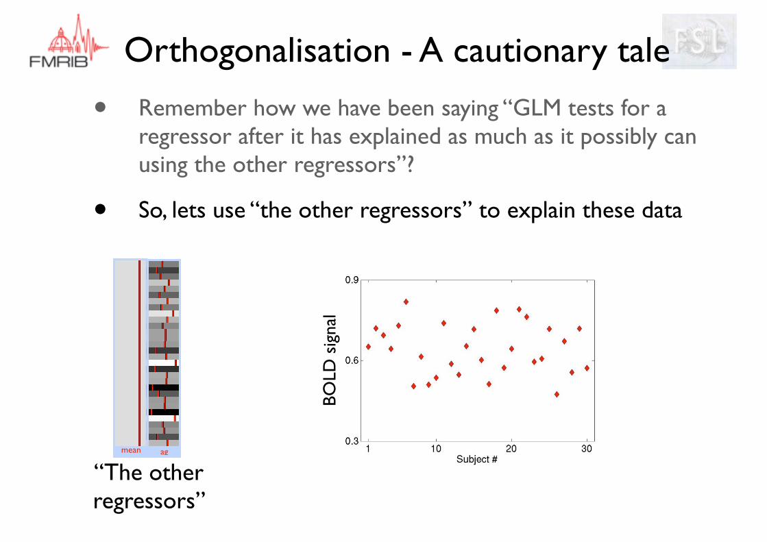
• Remember how we have been saying “GLM tests for a regressor after it has explained as much as it possibly can using the other regressors”?
• So, lets use “the other regressors” to explain these data
mean ag
“The other regressors”
BOLD
sig
nal
Orthogonalisation - A cautionary tale
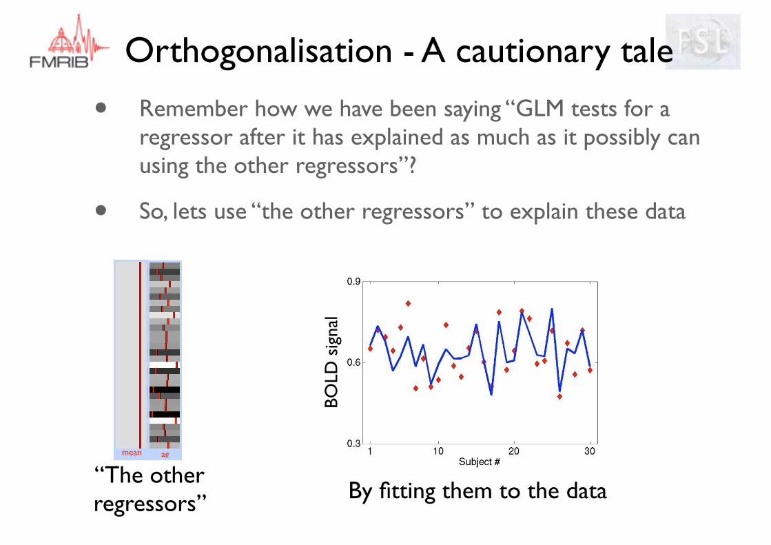
• Remember how we have been saying “GLM tests for a regressor after it has explained as much as it possibly can using the other regressors”?
• So, lets use “the other regressors” to explain these data
mean ag
“The other regressors” By fitting them to the data
BOLD
sig
nal
Orthogonalisation - A cautionary tale
• Remember how we have been saying “GLM tests for a regressor after it has explained as much as it possibly can using the other regressors”?
• And what is left is the “unexplained” part
“Explained” up to here
Unexplained
BOLD
sig
nal
Orthogonalisation - A cautionary tale
• Remember how we have been saying “GLM tests for a regressor after it has explained as much as it possibly can using the other regressors”?
• And what is left is the “unexplained” part
Original and “Explanation”“Unexplained”
(not well represented by DoD)
BOLD
sig
nal
Orthogonalisation - A cautionary tale
• Remember how we have been saying “GLM tests for a regressor after it has explained as much as it possibly can using the other regressors”?
• And the reason for all of this is that Age and DoD are correlated
• GLM says “I cannot be sure if this explanatory power belongs to you or to you. So neither can have it.”
• Much like a parent would.
Orthogonalisation - A cautionary tale
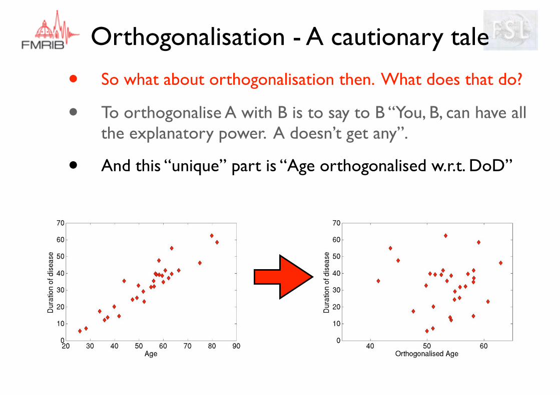
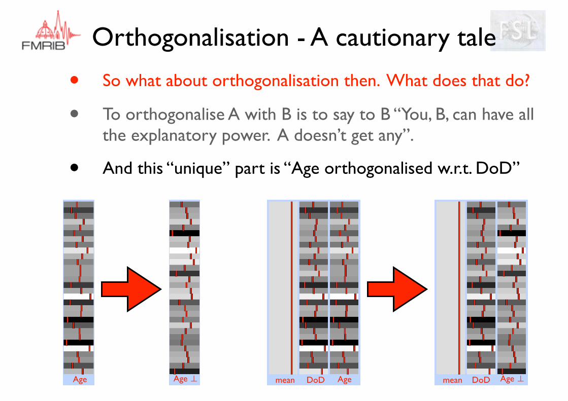
• So what about orthogonalisation then. What does that do?
• To orthogonalise A with B is to say to B “You, B, can have all the explanatory power. A doesn’t get any”.
• Let us see how we would orthogonalise Age w.r.t. DoD
DoD “explains” up to here
“Unexplained” − Unique to Age
Orthogonalisation - A cautionary tale
• So what about orthogonalisation then. What does that do?
• To orthogonalise A with B is to say to B “You, B, can have all the explanatory power. A doesn’t get any”.
• And this “unique” part is “Age orthogonalised w.r.t. DoD”
Orthogonalisation - A cautionary tale
• So what about orthogonalisation then. What does that do?
• To orthogonalise A with B is to say to B “You, B, can have all the explanatory power. A doesn’t get any”.
• And this “unique” part is “Age orthogonalised w.r.t. DoD”
Age Age ⊥ Agemean mean Age ⊥DoD DoD
Orthogonalisation - A cautionary tale• So what about orthogonalisation then. What does that do?
• To orthogonalise A with B is to say to B “You, B, can have all the explanatory power. A doesn’t get any”.
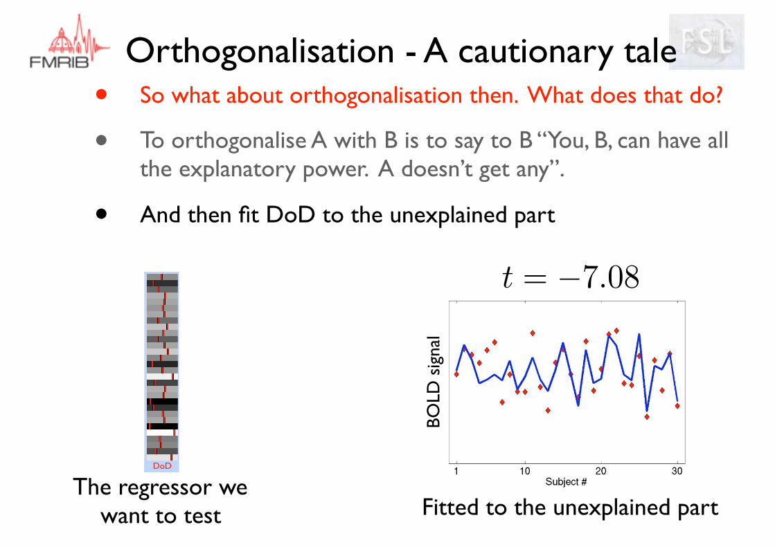
• And then fit DoD to the unexplained part
Fitted to the unexplained part
DoD
The regressor we want to test
t = �7.08
BO
LD s
igna
l
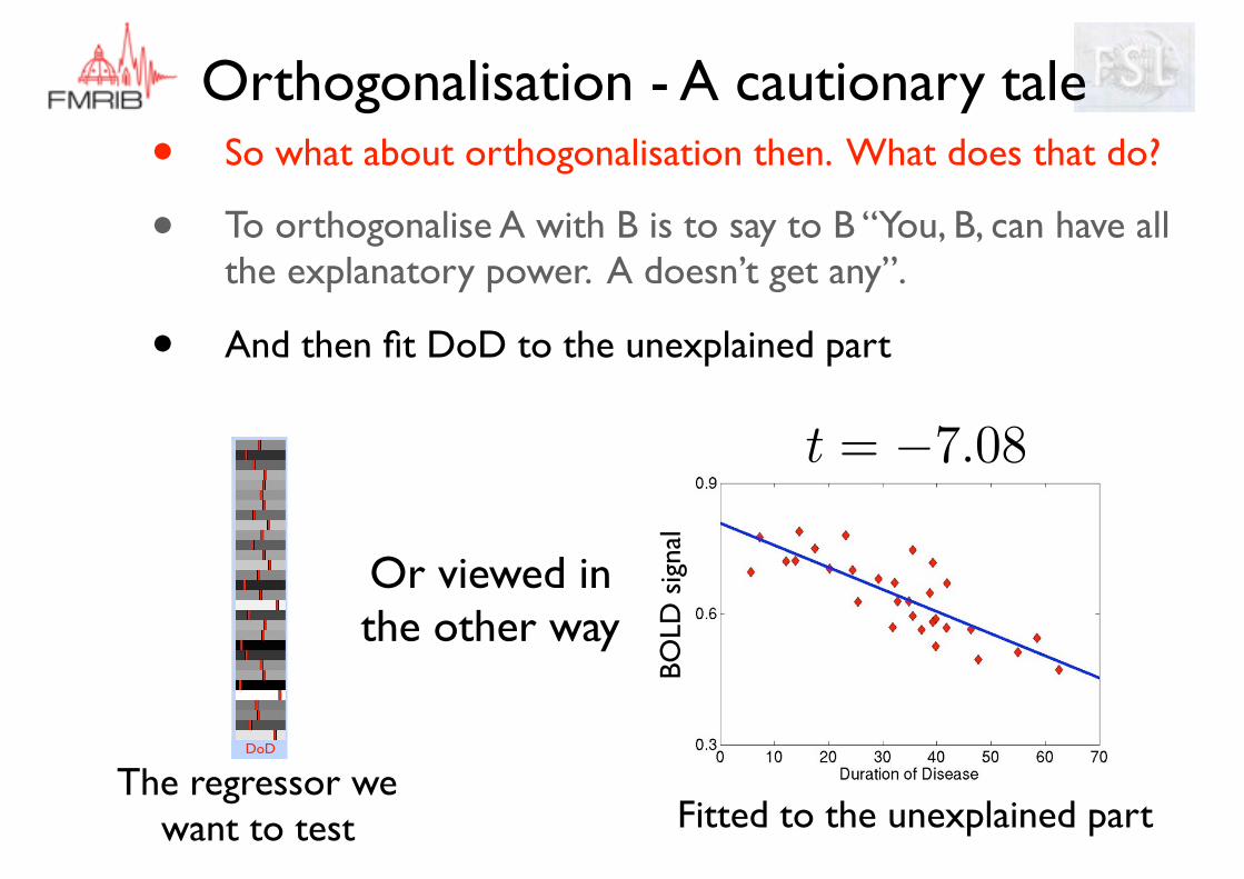
Orthogonalisation - A cautionary tale• So what about orthogonalisation then. What does that do?
• To orthogonalise A with B is to say to B “You, B, can have all the explanatory power. A doesn’t get any”.
• And then fit DoD to the unexplained part
Fitted to the unexplained part
DoD
The regressor we want to test
t = �7.08
Or viewed in the other way
BO
LD s
igna
l
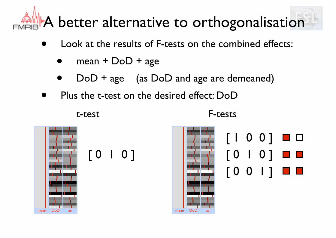
A better alternative to orthogonalisation• Look at the results of F-tests on the combined effects:
• mean + DoD + age
• DoD + age (as DoD and age are demeaned)
• Plus the t-test on the desired effect: DoD
mean DoD ag
[ 0 1 0 ]
t-test
mean DoD ag
[ 0 0 1 ][ 0 1 0 ][ 1 0 0 ]
F-tests
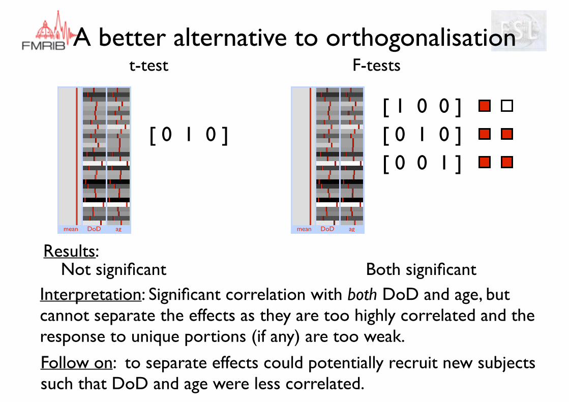
A better alternative to orthogonalisation
mean DoD ag
[ 0 1 0 ]
t-test
mean DoD ag
[ 0 0 1 ][ 0 1 0 ][ 1 0 0 ]
F-tests
Not significantResults:
Interpretation: Significant correlation with both DoD and age, but cannot separate the effects as they are too highly correlated and the response to unique portions (if any) are too weak.
Both significant
Follow on: to separate effects could potentially recruit new subjects such that DoD and age were less correlated.
Orthogonalisation - A cautionary tale
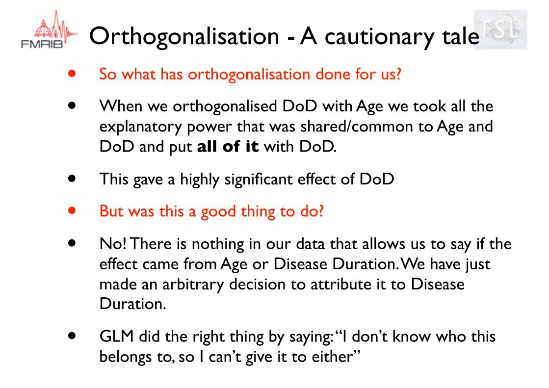
• So what has orthogonalisation done for us?
• When we orthogonalised DoD with Age we took all the explanatory power that was shared/common to Age and DoD and put all of it with DoD.
• This gave a highly significant effect of DoD
• But was this a good thing to do?
• No! There is nothing in our data that allows us to say if the effect came from Age or Disease Duration. We have just made an arbitrary decision to attribute it to Disease Duration.
• GLM did the right thing by saying: “I don’t know who this belongs to, so I can’t give it to either”
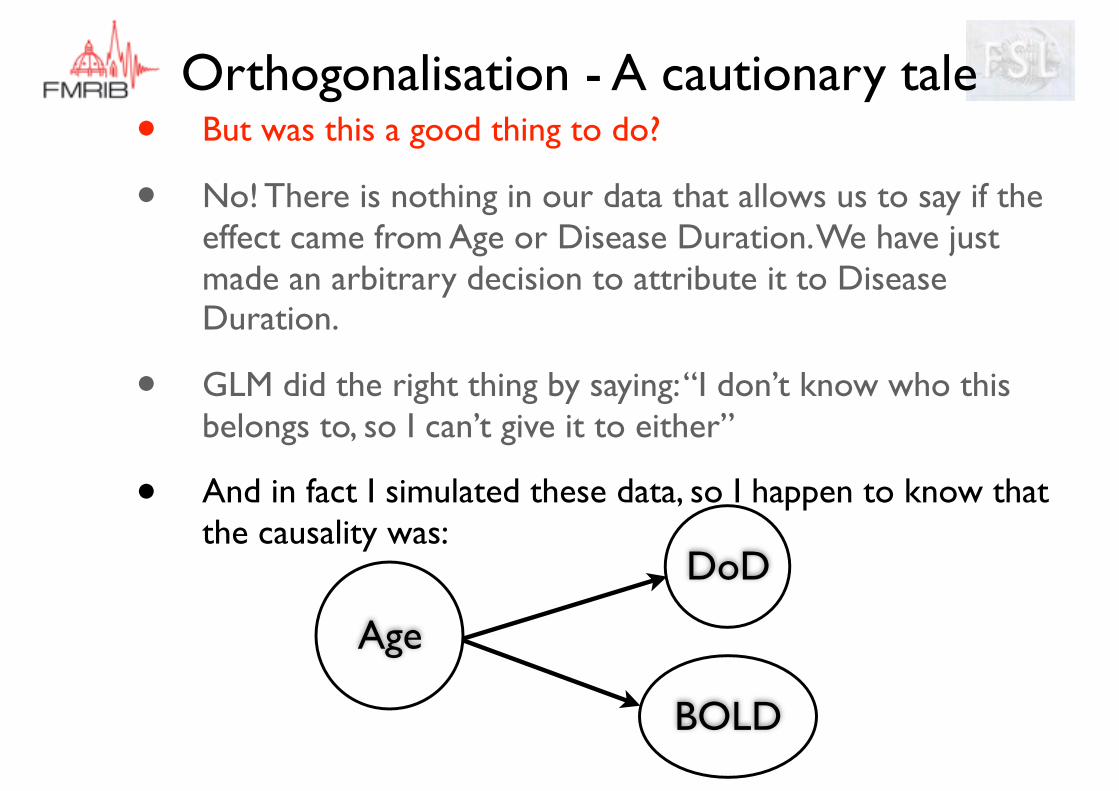
Orthogonalisation - A cautionary tale• But was this a good thing to do?
• No! There is nothing in our data that allows us to say if the effect came from Age or Disease Duration. We have just made an arbitrary decision to attribute it to Disease Duration.
• GLM did the right thing by saying: “I don’t know who this belongs to, so I can’t give it to either”
• And in fact I simulated these data, so I happen to know that the causality was:
Age
DoD
BOLD
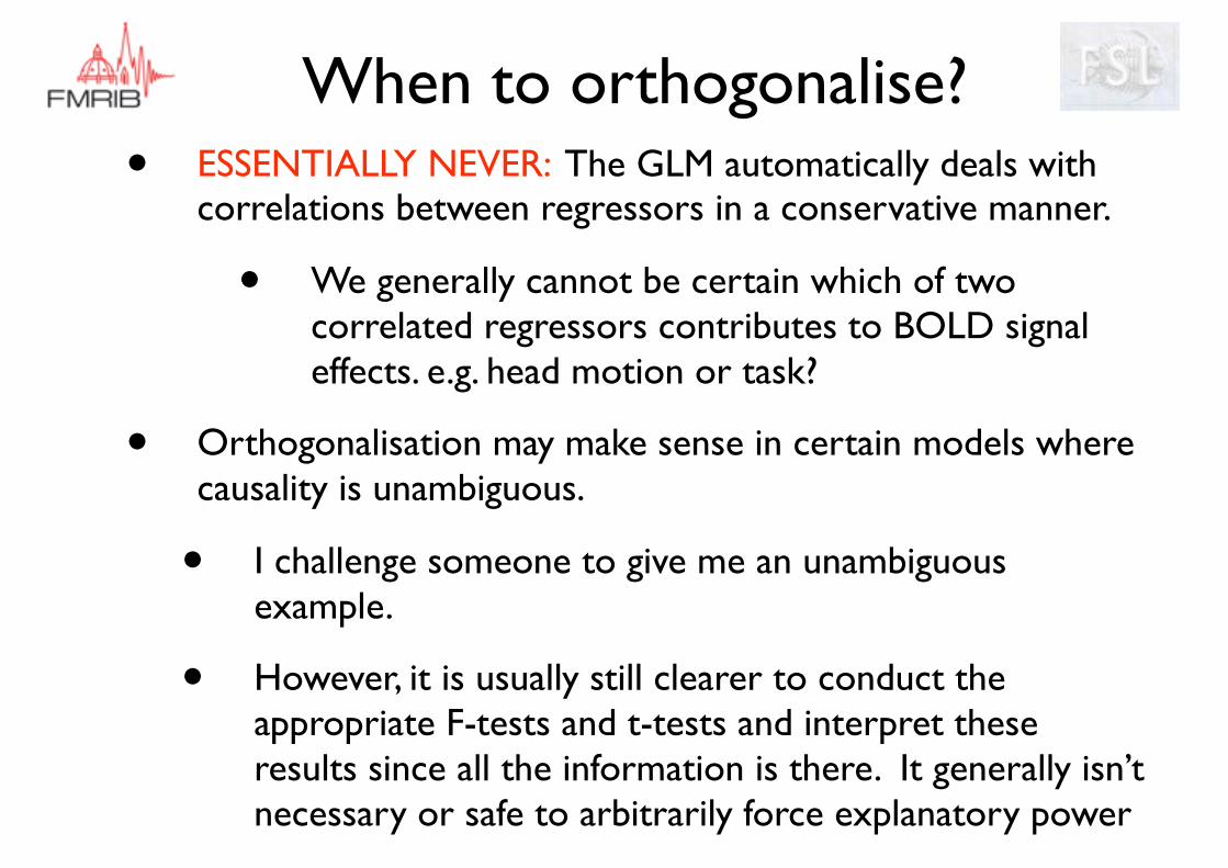
When to orthogonalise?• ESSENTIALLY NEVER: The GLM automatically deals with
correlations between regressors in a conservative manner.
• We generally cannot be certain which of two correlated regressors contributes to BOLD signal effects. e.g. head motion or task?
• Orthogonalisation may make sense in certain models where causality is unambiguous.
• I challenge someone to give me an unambiguous example.
• However, it is usually still clearer to conduct the appropriate F-tests and t-tests and interpret these results since all the information is there. It generally isn’t necessary or safe to arbitrarily force explanatory power
What does the fitted model look like?
ContrastDesign matrix
[ 1 -1 0 ]
[ 0 0 1 ]
[ 1 0 0 ]or
[ 0 1 0 ]Same slope in both groups
1 0 r11 0 r21 0 r30 1 r40 1 r50 1 r6
βG1βG2βr
Does demeaning change the
stats?
Demeaning recommended?
NO
NO
YES YES
YES
YES
mumford.fmripower.org/mean_centering/Demeaning
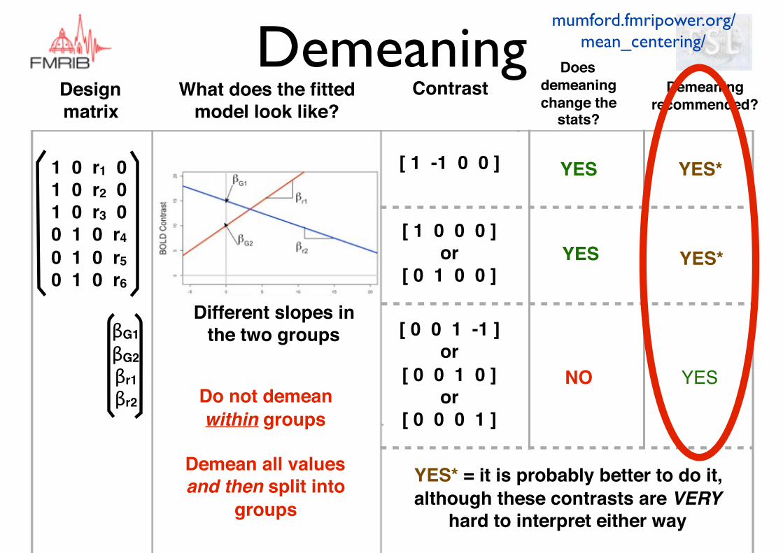
Does demeaning change the
stats?
What does the fitted model look like?
ContrastDesign matrix
[ 1 -1 0 0 ]
[ 1 0 0 0 ]or
[ 0 1 0 0 ]
[ 0 0 1 -1 ]or
[ 0 0 1 0 ]or
[ 0 0 0 1 ]
Different slopes in the two groups
1 0 r1 01 0 r2 01 0 r3 00 1 0 r40 1 0 r50 1 0 r6
βG1βG2βr1βr2
Demeaning recommended?
NO
YES
YES YES*
YES*
YESDo not demean within groups
Demean all values and then split into
groups
mumford.fmripower.org/mean_centering/
YES* = it is probably better to do it, although these contrasts are VERY
hard to interpret either way
Demeaning