feature engineering - ift6758.github.io
TRANSCRIPT

Feature EngineeringIFT6758 - Data Science
https://towardsdatascience.com/ways-to-detect-and-remove-the-outliers-404d16608dba
https://towardsdatascience.com/feature-engineering-for-machine-learning-3a5e293a5114
Sources:
https://www.slideshare.net/0xdata/feature-engineering-83511751

Announcements
• Midterm: October 31 at 16:30 – 18:30 (those who cannot make it at 16:30, send us an email asap. We will arrange a room for them to do the same exam at 14:30 – 16:30)
• Project evaluation: The teams with the results same as baseline on the scoreboard for Evaluation1 got the full grade for the first project assignment, i.e., User05, User06, User08, User09, User14, User17, User22, User25, User26, User29, User30.
• The other teams will be graded this week based on their scores for Evaluation 2.
• We have two invited talks next week on Tuesday (Geospatial and Time series data analysis) and Thursday (Privacy and Transparency in Machine Learning).
• Project Presentation will take place on November 5
!2

Feature Engineering
!3
Data scientists usually spend the most time on feature engineering!

Feature engineering cycle
!4
Not Feature Engineering
• data collection
• Creating the target variable
• Removing duplicates
• Fixing mislabeled classes.

Feature engineering cycle
!5

Feature engineering cycle
!6

Feature engineering is hard
• Powerful feature transformations (like target encoding) can introduce leakage when applied wrong
• Usually requires domain knowledge about how features interact with each other
• Time-consuming, need to run thousand of experiments
• Why Feature Engineering matters
• Extract more new gold features, remove irrelevant or noisy features
• Simpler models with better results
!7

Key Elements of Feature Engineering
!8
Target Transformation
Feature Encoding
Feature Extraction

Target Transformation
• Predictor/Response Variable Transformation
• Use it when variable shows a skewed distribution make the residuals more close to “normal distribution” (bell curve)
• Can improve model fite.g., log(x), log(x+1), sqrt(x), sqrt(x+1), etc.
!9

Target Transformation
!10

Key Elements of Feature Engineering
!11
Target Transformation
Feature Encoding
Feature Extraction

Imputation
• Common problem in preparing the data: Missing Values
• Why we have missing values?
• Human errors
• Interruptions in the data flow
• Privacy concerns
• What to do?
!12

Imputation
• Common problem in preparing the data: Missing Values
• Why we have missing values?
• Human errors
• Interruptions in the data flow
• Privacy concerns
• What to do?
• Simple solution: drop the row/column
• Preferable option: Imputation
!13

Imputation
• Numerical Imputation
• Assing zero
• Assing NA
• Default value or medians of the columns (Note that averages are sensitive to outlier values)
• Categorical Imputation
• maximum occurred value
• There is not a dominant value, imputing a category like “Other”
!14

Outliers
Outliers may introduce to the population during data collections
!15
mistake ?
variance ?

Outlier detection
• Outlier: A data object that deviates significantly from the normal objects as if it were generated by a different mechanism Ex.: Unusual credit card purchase, sports: Michael Jordon, Wayne Gretzky, …
• Outliers are different from the noise dataNoise is random error or variance in a measured variableNoise should be removed before outlier detection
• Outliers are interesting: It violates the mechanism that generates the normal data Outlier detection vs. novelty detection: early stage, outlier; but later merged into the model
• Applications:Credit card fraud detectionTelecom fraud detection Customer segmentationMedical analysis
!16

Types of Outliers
!17
■ Three kinds: global, contextual and collective outliers ■ Global outlier (or point anomaly)
■ Object is Og if it significantly deviates from the rest of the data set■ Ex. Intrusion detection in computer networks■ Issue: Find an appropriate measurement of deviation
■ Contextual outlier (or conditional outlier)■ Object is Oc if it deviates significantly based on a selected context■ Ex. 80o F in Urbana: outlier? (depending on summer or winter?)■ Attributes of data objects should be divided into two groups
■ Contextual attributes: defines the context, e.g., time & location ■ Behavioral attributes: characteristics of the object, used in outlier
evaluation, e.g., temperature■ Can be viewed as a generalization of local outliers—whose density
significantly deviates from its local area■ Issue: How to define or formulate meaningful context?

Types of Outliers
!18
■ Collective Outliers ■ A subset of data objects collectively deviate significantly from the whole data
set, even if the individual data objects may not be outliers■ Applications: E.g., intrusion detection:
■ When a number of computers keep sending denial-of-service packages to each other
■ Detection of collective outliers■ Consider not only behavior of individual objects, but also that of groups of
objects■ Need to have the background knowledge on the relationship among data
objects, such as a distance or similarity measure on objects.■ A data set may have multiple types of outlier■ One object may belong to more than one type of outlier

Finding Outliers
• To ease the discovery of outliers, we have plenty of methods in statistics:
• Discover outliers with visualization tools or statistical methodologies
• Box plot
• Scatter plot
• Z-score
• IQR score
We will cover more advanced techniques for anomaly detection (after the mid-term)
!19

Finding Outliers
Box plot
• This definition suggests, that if there is an outlier it will plotted as point in boxplot but other population will be grouped together and display as boxes.
!20
In descriptive statistics, a box plot is a method for graphically depicting groups of numerical data through their quartiles. Box plots may also have lines extending vertically from the boxes (whiskers) indicating variability outside the upper and lower quartiles, hence the terms box-and-whisker plot and box-and-whisker diagram. Outliers may be plotted as individual points.
Wikipedia Definition

Finding Outliers
• Box plot
!21

Finding Outliers
• Above plot shows three points between 10 to 12, these are outliers as there are not included in the box of other observation i.e no where near the quartiles.
• Here we analysed Uni-variate outlier i.e. we used DIS column only to check the outlier.
• We can do multivariate outlier analysis too. Can we do the multivariate analysis with Box plot? Well it depends, if you have a categorical values then you can use that with any continuous variable and do multivariate outlier analysis.
!22

Finding Outliers
A scatter plot , is a type of plot or mathematical diagram using Cartesian coordinates to display values for typically two variables for a set of data. The data are displayed as a collection of points, each having the value of one variable determining the position on the horizontal axis and the value of the other variable determining the position on the vertical axis.
Wikipedia Definition
Scatter plot
• This definition suggests, the scatter plot is the collection of points that shows values for two variables.
!23

• We can try and draw scatter plot for two variables from our housing dataset.
!24
Finding Outliers

• Looking at the plot above, we can most of data points are lying bottom left side but there are points which are far from the population like top right corner.
!25
Finding Outliers

Standard deviation
!26
Finding Outliers
In statistics, the standard deviation (SD, also represented by the lower case Greek letter sigma σ for the population standard deviation or the Latin letter s for the sample standard deviation) is a measure of the amount of variation or dispersion of a set of values.
Wikipedia Definition

• If a value has a distance to the average higher than x * standard deviation,it can be assumed as an outlier. Then what x should be?
• Usually, a value between 2 and 4 seems practical.
!27
Finding Outliers

Z-score
• The intuition behind Z-score is to describe any data point by finding their relationship with the Standard Deviation and Mean of the group of data points. Z-score is finding the distribution of data where mean is 0 and standard deviation is 1 i.e. normal distribution.
!28
Finding Outliers
The Z-score is the signed number of standard deviations by which the value of an observation or data point is above the mean value of what is being observed or measured.
Wikipedia Definition

• Z-score: While calculating the Z-score we re-scale and center the data and look for data points which are too far from zero. These data points which are way too far from zero will be treated as the outliers. In most of the cases a threshold of 3 or -3 is used i.e if the Z-score value is greater than or less than 3 or -3 respectively, that data point will be identified as outliers.
• We will use Z-score function defined in scipy library to detect the outliers.
!29
Finding Outliers

• Looking the code and the output above, it is difficult to say which data point is an outlier. Let’s try and define a threshold to identify an outlier.
!30
Finding Outliers
List of arrow numbers
List of Column numbers

IQR score
• It is a measure of the dispersion similar to standard deviation or variance, but is much more robust against outliers.
!31
Finding Outliers
The interquartile range (IQR), also called the midspread or middle 50%, or technically H-spread, is a measure of statistical dispersion, being equal to the difference between 75th and 25th percentiles, or between upper and lower quartiles, IQR = Q3 − Q1.
Wikipedia Definition

• Let’s find out we can box plot uses IQR and how we can use it to find the list of outliers as we did using Z-score calculation. First we will calculate IQR
!32
Finding Outliers

• The data point where we have False that means these values are valid whereas True indicates presence of an outlier.
!33
Finding Outliers

Percentiles
•Another mathematical method to detect outliers is to use percentiles.
•You can assume a certain percent of the value from the top or the bottom as an outlier.
•A common mistake is using the percentiles according to the range of the data, e.g., if your data ranges from 0 to 100, your top 5% is not the values between 96 and 100. Top 5% means the values that are out of the 95th percentile of data.
!34
Finding Outliers

Handling Outliers
An Outlier Dilemma: Drop or Cap
• Correcting
• Removing
• Z-score:
• IQR score:
!35

Binning
• Binning can be applied on both categorical and numerical data:
• Example
!36

• The main motivation of binning is to make the model more robust and prevent overfitting, however, it has a cost to the performance.
• The trade-off between performance and overfitting is the key point of the binning process.
• Numerical binning: binning might be redundant due to its effect on model performance.
• Categorical binning: the labels with low frequencies probably affect the robustness of statistical models negatively. Thus, assigning a general category to these less frequent values helps to keep the robustness of the model.
!37
Binning

Log Transformation
• Logarithm transformation (or log transform):
• It helps to handle skewed data and after transformation, the distribution becomes more approximate to normal.
• In most of the cases the magnitude order of the data changes within the range of the data.
• It also decreases the effect of the outliers, due to the normalization of magnitude differences and the model become more robust.
!38

• The data you apply log transform must have only positive values, otherwise you receive an error. Also, you can add 1 to your data before transform it. Thus, you ensure the output of the transformation to be positive.
!39
Log Transformation

Grouping
• Tidy data where each row represents an instance and each column represent a feature.
• Datasets such as transactions rarely fit the definition of tidy data -> we use grouping.
• The key point of group by operations is to decide the aggregation functions of the features.
!40

• Aggregating categorical columns:
• Highest frequency: the max operation for categorical columns
• Make a Pivot table: This would be a good option if you aim to go beyond binary flag columns and merge multiple features into aggregated features, which are more informative.
• Apply one-hot encoding
!41
Grouping

• Numerical columns are mostly grouped using:
• Sum
• Mean
!42
Grouping

Splitting
• Most of the time the dataset contains string columns that violates tidy data principles.
• Split function is a good option, however, there is no one way of splitting features
!43

Scaling
• In most cases, the numerical features of the dataset do not have a certain range and they differ from each other.
• In real life, it is nonsense to expect age and income columns to have the same range. But from the machine learning point of view, how these two columns can be compared?
• It is important for algorithms that work based on distance: such as k-NN or k-Means
• Basically, there are two common ways of scaling: Normalization, and Standardization
!44

Normalization
• Normalization (or min-max normalization) scale all values in a fixed range between 0 and 1.
• This transformation does not change the distribution of the feature.
• But due to the decreased standard deviations, the effects of the outliers increases. So before normalization, it is recommended to handle the outliers.
!45

• Example:
!46
Normalization

Standardization
• Standardization (or z-score normalization) scales the values while taking into account standard deviation.
• In the following formula of standardization, the mean is shown as μ and the standard deviation is shown as σ.
• If the standard deviation of features is different, their range also would differ from each other. This reduces the effect of the outliers in the features.
!47

• Example:
!48
Standardization

Key Elements of Feature Engineering
!49
Target Transformation
Feature Encoding
Feature Extraction

Feature Encoding
• Turn categorical features into numeric features to provide more fine-grained information
• Help explicitly capture non-linear relationships and interactions between the values of features
• Most of machine learning tools only accept numbers as their input e.g., xgboost, gbm, glmnet, libsvm, liblinear, etc.
!50

• Labeled EncodingInterpret the categories as ordered integers (mostly wrong) Python scikit-learn: LabelEncoder • Ok for tree-based methods
• One Hot EncodingTransform categories into individual binary (0 or 1) features Python scikit-learn: DictVectorizer, OneHotEncoder • Ok for K-means, Linear, NNs, etc.
!51
Feature Encoding

One Hot Encoding
• One-hot-encoding: is one of the most common encoding methods in machine learning.
• This method spreads the values in a column to multiple flag columns and assigns 0 or 1 to them. These binary values express the relationship between grouped and encoded column.
!52

Frequency encoding
• Encoding of categorical levels of feature to values between 0 and 1 based on their relative frequency
!53

Target mean encoding
• Instead of dummy encoding of categorical variables and increasing the number of features we can encode each level as the mean of the response.
!54

• It is better to calculate weighted average of the overall mean of the training set and the mean of the level:
• The weights are based on the frequency of the levels i.e. if a category only appears a few times in the dataset then its encoded value will be close to the overall mean instead of the mean of that level.
!55
Target mean encoding

!56
Target mean encoding Smoothing

!57
Target mean encoding Smoothing

Target mean encoding leave-one-out schema
• To avoid overfitting we could use leave-one-out schema
!58

Target mean encoding leave-one-out schema
• To avoid overfitting we could use leave-one-out schema
!59

Target mean encoding leave-one-out schema
• To avoid overfitting we could use leave-one-out schema
!60

Target mean encoding leave-one-out schema
• To avoid overfitting we could use leave-one-out schema
!61

Target mean encoding leave-one-out schema
• To avoid overfitting we could use leave-one-out schema
!62

Weight of Evidence and Information Value
• Weight of evidence:
• To avoid division by zero:
• Information Value:
!63

Weight of Evidence and Information Value
!64
0.221
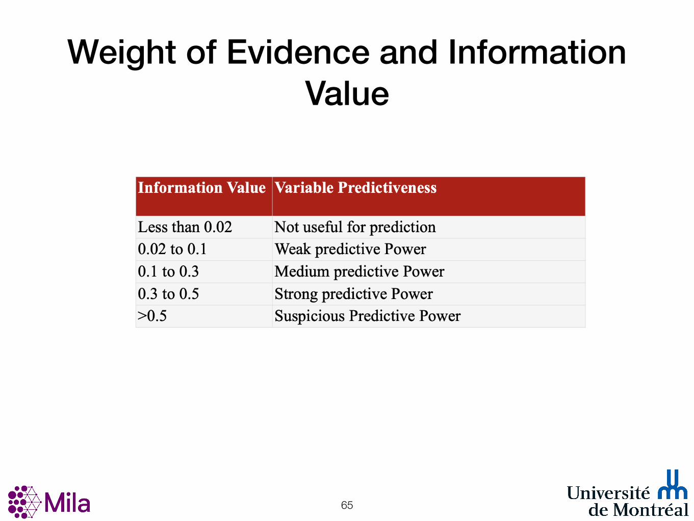
Weight of Evidence and Information Value
!65

More of Feature Engineerings …
• Feature Extraction: Numerical data• Dimensionality reduction techniques – SVD and PCA (Week 3)• Clustering and using cluster IDs or/and distances to cluster centers as new features (Week 3) • Feature selection (Week 6)
• Feature Extraction: Textual data (Week 10) • e.g., Bag-of-Words: extract tokens from text and use their occurrences (or TF/IDF weights) as features
• Feature Extraction: Time series and GEO location (Week 7)
• Feature Extraction: Image data (Week 11)
• Feature Extraction: Relational data (Week 12)
• Anomaly detection (advanced): (Week 13)
!66