Feature Extraction for Time Series Data: an Artificial Neural Network Evolutionary Training Model for the Management of Mountainous Watersheds.

Thomas J. Glezakos1, Theodore A. Tsiligiridis1, Lazaros Iliadis2, Constantine P. Yialouris1, Fotis Maris2, Konstantinos P. Ferentinos1

1Agricultural University of Athens, Department of Science, Laboratory of Informatics, 75 Iera Odos street, 11855, Athens, Hellas

2Democritus University of Thrace, Department of Forestry & Management of the Environment & Natural Resources,193 Pantazidou street, 68200 Orestiada, Thrace, Hellas

Abstract The present manuscript is the result of research conducted towards a wider use of Artificial Neural Networks in the management of mountainous water supplies. The novelty lies on the evolutionary clustering of time series data which are then used for the training and testing of a neural object, applying meta – heuristics in the neural training phase, for the management of water resources and for torrential risk estimation and modelling. It is essentially an attempt towards the development of a more credible forecasting system, exploiting an evolutionary approach used to interpret and model the significance which time series data pose on the behavior of the aforementioned environmental reserves. The proposed model, designed such as to effectively estimate the Average Annual Water Supply for the various mountainous watersheds, accepts as inputs a wide range of meta - data produced via an evolutionary genetic process. The data used for the training and testing of the system refer to certain watersheds spread over the island of Cyprus and span a wide temporal period. The method proposed incorporates an evolutionary process to manipulate the time series data of the average monthly rainfall recorded by the measuring stations, while the algorithm includes special encoding, initialization, performance evaluation, genetic operations and pattern matching tools for the evolution of the time series into significantly sampled data.

Keywords: Genetic algorithms; Artificial Neural Networks; Maximum volume of water flow; Average Annual Water Supply; Evolutionary time series processing; Genetic ANN training.

1. Introduction

The most common reason for a flood surge at a certain time and space is the condition at which bodies of water overflow, or tides rise inexorably, due to a significant amount of rainfall or, for some reason, an excessive snow thawing, which overloads the water capacities of nearby natural or artificial reservoirs. Flood is defined by the National Flood Insurance Program [57] as an excess of water on land that is normally drier, or a general and temporary condition of partial or complete inundation of two or more acres of normally dry land area from overflow of inland or tidal water, or unusual and rapid accumulation or runoff of surface waters from any source, or mudflow, or collapse or subsidence of land along the shore of a lake or similar body of water as a result of erosion or undermining caused by waves or currents of water exceeding anticipated cyclical levels. Also, it is not necessary for a flood to happen near vast bodies of water. Flash floods can happen everywhere, independently of altitude, longitude or latitude, when large volumes of rainfalls happen within a short period of time in the same area. It is also common knowledge that torrential streams which overflow and run wild, can cause heavy floods, which become more dangerous as the ability of the soil to absorb water diminishes and as the average annual rain height increases. The flow and the power of the torrential stream is not so much dependant on the amount of water precipitation, as it is on its peaks at certain periods of the year. The fact that torrential surges happen at certain seasonal intervals has made the researchers contemplate on its analysis on various data sets accumulated in various ways. It is nowadays made clear that the water resources of a country play

one of the lead roles in the well - being of its citizens and are very important for its sustainable development, while their management is considered a crucial issue. The most profound way to manage the flow of torrential streams and the flood risk they pose on the environment is delivered by time series analysis, where the monthly rainfall is considered as the most basic element. Other factors are considered as well, such as the landscape type and structure, the altitude of the stream, the surface of the watershed, the land use and land cover and so on, but they are not as crucial as the time series one. The analysis of time series, most of the time resorts to regression models, such as the autoregressive and the moving average methods [30], which more often than not are inhibited by the non-linearity inherent in the input time series data. Various fault-tolerant tools, such as fuzzy systems and neural networks have been engaged [5] [14–17] [24] [27] [33] [37] [42] [50–53] in order to address this problem. Also, a lot of research has been dedicated in studying the development and prototyping of neural network design or the training and testing via meta – heuristic methods [1] [13] [34] [36] [40] [45]. The dimensionality of the input data vector has been contemplated a lot in this context and has been found to be most crucial for this kind of data analysis. Most of the researchers agree that in case the dimensionality may be delivered too small, the neural network might not have all the important information at its disposal. On the other hand, if the dimensionality rises at high levels, then we run the risk of over - feeding the network, which might result in redundant information and noise creeping into it, inhibiting its function, causing over - fitting and smothering its ability to generalize [30]. The present manuscript describes the design, implementation and testing of an innovative method to control the dimensionality of the input data vector, by producing time series meta - data used as inputs to a neural network to predict torrential risk. The meta-data production is achieved in an evolving fashion, via a genetic algorithm which manipulates the input dimension of the time – series. Thus, the algorithm is enabled to fluctuate and statistically manipulate the time interval between two, not necessarily successive, elements of the series which are to be fed into the network. It then utilizes the overall root mean square (RMS) error of the network to formulate the fitness function, while the roulette wheel method is engaged so as to develop the selection policy for the next generation of the population of the algorithm.

1.1 The artificial neural network concept and its implementation in torrential risk management

The human brain is a highly complicated biologic machine, capable of solving innumerable kinds of problems, from the most simplistic to highly complex ones. The Artificial Neural Network (ANN) concept was developed in an attempt to simulate the wondrous function of the human brain. An ANN is a software device consisting of a number of simple processing elements interconnected and operating in parallel. Each neuron is only aware of the signals it receives from other connected neurons and the information it sends from time to time to other processing elements. In this context, an ANN is a computer program capable of learning from examples through iteration. Most of the times no prior knowledge of the input data is required, for the training process is essentially a search for the best synaptic weight vector. Learning is the process of adapting or modifying the neurons’ connection weights in response to stimuli presented as inputs requiring the presence of a known output. This process enables the network to learn to solve problems by adequately adjusting the strength of the connections between their processing elements according to the input data and the desired outputs. Thus, a neural network may learn by example and outmatches rivalling techniques in that it may use its knowledge under untrained circumstances incorporating a large number of variables [18]. Such kind of software devices, have been vastly used for recognizing patterns in the input data space or to extract simple rules for complex non linear problems according to their inputs. The key factor and primary goal in neural network training is generalization. The term refers to the capability of the network to predict “unseen” inputs merely with the knowledge that has been acquired during training. This is a process in which a result emerging in the output corresponds to a desired response for a given input stimulus. The ANN concept is currently widely used in various research works, ranging from pattern recognition, quality control and classification, gaining wide recognition by its ability to model numerous processes in engineering [6] [19] [25] [35] [41] [48]. Lately they have been used to predict wood water isotherm or sorption isotherms in food science [4] [32] and in numerous other disciplines. Their fault tolerant behaviour, as well as their ability to process non linear problems and generalize on unseen information has not gone unseen by the water resources management research. The transition to a more potent and effective research tool was also dictated by the dramatic climatic change happening during the recent years. This is

considered to be responsible for a lot of distinctively catastrophic calamities all over the world. In [5], Bodri and Cermak developed a predictive approach based on modelling flood recurrence via Artificial Neural Networks to contribute in flood management of the eastern part of the Czech Republic, Moravia, which was seriously pelted during the 1997 Central European floods. In [50], Toth et al. compared the accuracy of the short term rainfall forecasts obtained with time series analysis techniques, using past rainfall depths as the only input. Their study compared the linear stochastic auto – regressive moving average models, artificial neural networks and the non – parametric nearest neighbour method, concluding that the neural network time series analysis provides a significant improvement in flood forecasting accuracy. Wei et al. in [51] developed a potent neural network approach to provide accurate flood disaster predictions in China. Their model is intended at providing a system able to manipulate non ideal time series data. Ni and Xue in [33] developed a Radial Basis Function Artificial Neural Network to provide accurate flood risk forecasting and ranking in five safety polders in the upper catchments of the Yangtze River in China, which has undergone vast ecological pressure due to intensified human activity during the recent years. Filho and dos Santos compared the ability of Artificial Neural Networks and multi – parameter auto – regression models [14]. Their model is fed into with time series data so as to simulate and forecast stage level and stream flow at Tamanduatei River watershed in Sao Paulo of Brazil. The research shows that the ANN approach is slightly better than the auto – regression one and indicates its usefulness in flash flood forecasting. Harpham and Dawson [17] studied the variation of test set error among six different recognised basis functions used in Radial Basis Functions Artificial Neural Networks. The tests were carried out on various time series flood prediction data sets for the Rivers Amber and Mole, in United Kingdom. In [27], Kerh and Lee engaged a neural network approach so as to forecast flood discharge at a station downstream of Kaoping River. The input to the network was information obtained by stations situated upstream of the river, while there was no available information at the flood location. Their verification results showed that the neural network model outperforms the conventional Muskingum method which is widely used for flood routing in natural channels and rivers. In [37] Pulido – Calvo and Portela, as well as Sahoo et al. in [42], developed similar models to forecast torrential flows at various Portuguese and Hawaiian watersheds respectively, concluding that the neural network approach is the most promising among the ones studied. Finally, Jain and Kumar [24] proposed a hybrid neural network model combining the strengths of conventional and neural techniques for time series forecasting using the monthly stream flow data available for the Colorado River at Lees Ferry in the United States of America.

1.2 Genetic Algorithms in water resources management

The genetic algorithm concept was inspired by evolutionary biology, and specifically driven by the Darwinian axiom of the “survival of the fittest”, incorporating numerous biological procedures such as inheritance, selection, recombination (or crossover) and mutation. They became popular through the work of John Holland, particularly his 1975 book “Adaptation in Natural and Artificial Systems”. Such algorithms are mostly implemented as computer simulations which search for optimal solutions to a given optimization problem. The genetic algorithm starts out with an, often random, initial population of encoded representations of candidate solutions. These representations are referred to as chromosomes, genotypes or genome, while the candidate solutions are referred to as phenotypes. The algorithm proceeds by generations each of which is comprised by genotypes of the previous generation, which are elected basically by their fitness and modified on the grounds of a possible recombination or mutation to form a new population of higher overall fitness. There are numerous applications of genetic algorithms in water resources management in general. In [7] Cai et al., combined GAs with linear programming so as to propose feasible solutions to large scale water resources management problems. Their work aims at smoothing out the complex variables of the problem, rendering it linear in its remaining variables, which are then varied by the genetic algorithm. In [10], Cheng et al., proposed a combination of fuzzy systems and genetic algorithms to solve the calibration problem of multi-objective rainfall – runoff models in the Shuangpai Reservoir in China. In their model, genetic algorithms are used in the calibration both of water balance and of runoff routing parameters. The same researcher returns in [11] with a further development of his previous work using an enhanced version of his genetic algorithm to overcome the difficulty of recognizing the model’s best behaviours during the calibration procedure. Agrawal and Singh in [2] used the same algorithms to develop and optimize a runoff prediction model for the Kashinagar watershed of the Vamsadhara river basin in Orissa of India. The genetic algorithms are used in this concept for the estimation of the model parameters and for function

optimization. Based on the grounds that watershed modelling is essential for the management of water resources and that it requires proper description of rainfall spatial variation, Chang et al., proposed in [8] a model which utilizes a genetic algorithm to determine the parameters of fuzzy membership functions representing locations without rainfall records to their surrounding rainfall gauges. The results of the work clearly show a reduction of the estimated error when genetic algorithms are employed. Neural Network evolutionary training has been studied a lot as regards to water resources management. In [49], Srinivasulu and Jain compared three different neural network training techniques for rainfall – runoff modelling, one of which was using a genetic algorithm to formulate the training pairs and the other being normal back propagation. A Self Organizing Map (SOM) was used to classify the input/output space into different categories, before developing neural networks for each one. The results of the work show that the genetic algorithm technique easily outperforms normal back propagation. During the same period, Anctil et al. [3] proposed a neural model of improved forecasting ability through the optimization of the mean daily rainfall time series, which was achieved by the implementation of a genetic algorithm. More recently, in 2007, Chau developed a split – step particle swarm optimization model to train multi layered perceptrons so as to forecast real time water levels at Fo Tan in Shing Mun River in Hong Kong [9]. His results exhibit enhanced accuracy when compared to benchmarking back propagation. During the same year, Kerachian and Karamouz [26] developed a stochastic conflict resolution technique based on genetic algorithms which, combined to a water quality simulation system, was able to model reservoir operation and waste load allocation for the Ghomrud Reservoir River System in the central part of Iran. Finally, Damle and Yalcin describe in [12] a novel approach to river flood prediction using time series data mining procedures. These, among others, employ a genetic algorithm to search for optimal pattern clusters in the data set. Their method was successfully used in St. Louis gauging station located on the Mississippi River in the United States of America.

2. Case Study: the area and the problem

Cyprus, the third largest island in the Mediterranean Sea after Sicily and Sardinia, is geographically situated in the east, south of the Anatolian Peninsula of the Asian mainland. It is located among Hellas to its west / north-west side, Syria, Lebanon and Israel to the east, and Turkey at north. Although commonly referred to as part of the Middle East, it is closely alligned with Europe [55]. The landscape, mostly mountainous at the highest percentage, includes the central plain of Mesaoria, with the Kyrenia and Pentadactylos mountains to the north and the Troodos mountain range to the south and west, while there are also scattered, but significant, plains along the southern coast. The climate is temperate Mediterranean where dry summers follow variably rainy winters. Summer temperatures range from warm at higher elevations in the Troodos mountains to hot in the lowlands. Winter temperatures are mild at lower elevations, where snow rarely occurs, but are significantly colder in the Troodos mountains. During the recent years the dry seasons are intense, rendering the lack of drinking water as a high pressure on the citizens. On the other hand, floods, lower temperatures and torrential rains throughout the wet season constitute an unusual picture for this time of year for the island [54], causing erosion problems and destroy settlements and infrastructure. There is no doubt whatsoever that proper and efficacious water management is the key factor not only for the well being of the citizens and the satisfaction of their daily needs, but for the achievement of sustainable development as well. The primary aim of the present research is to present an attempt towards the design and implementation of an evolutionary technique in the line of producing meta-data for the training and testing of Artificial Neural Networks (ANN) for the management of water reservoirs. The motivation for our research was triggered off by [21] and [22]. According to these works, it is beyond doubt that an innovative approach may come in handy, especially considering the fact that after time – consuming studies and raw data acquisition, the Republic of Cyprus did not come up with a viable solution to the problem of water resources management. In [22], Iliadis and Maris state that the classical statistical analysis failed to provide promising results, although newer attempts have been conducted towards this purpose. The recent findings of the undergoing research have revealed that the water resources of the island are much lower than it was initially regarded. It is nowadays estimated that the island’s water reservoir is approximately 40% lower than the original belief. This fact urges for a new and perhaps more reliable approach. The current research focuses on producing meta - data out of raw time series data, in the hope of eliminating the noise inherent in the initial information. This procedure is followed in order to develop a highly adaptive evolutionary model towards decision making in water resources management. The genetic

algorithm governing the meta - data production performs a forward crawl through the input space in search of combination of genes which outperform their brethren after they have been used as inputs to the neural network, the performance of which is evaluated by means of its root mean square error. The network performs an effective estimation of the Average Annual Water Supply (AAWS) on an annual basis, for each mountainous watershed of Cyprus. The estimation of the aforementioned factor plays a highly important role to the management of mountainous water resources, as it is closely related to the mountainous watershed fermentations, as well as to the potential torrential risks posed on the areas involved [21] [23] [46] [47].

3. Materials and Methods

3.1. Research Area and data acquisition

The research area, as in the initial research [22], covers all of the mountainous watersheds which are under the administration of the Republic of Cyprus. Specifically, the island is divided into nine water Divisions with a total of seventy Torrential Streams. As already noted, the two most important landscape characteristics of the island are the Kyrenia and Pentadactylos mountains to the north with an altitude which reaches 1000 m. and a length of 160 km., and the Troodos mountain range to the south and west with a maximum altitude of 1951 m.

20

Scale

40 Km0

Watershed Boundary

Hydrological Region Boundary

2

1 9

3

8

4

6

1 Hydrological Region Number

7

5

Ammochostos

Larnaka

Keryneia

Lefkosia

Lemesos

Pafos

Polis

No data available - Area under Turkish occupation

58 stream-flow stations used in the analysis

2-2-3-95

2-2-6-60

2-3-4-95

2-2-8-95 2-3-4-80

1-1-7-95

1-2-7-90

1-4-9-80 1-3-8-55

1-4-7-10

2-4-6-80

1-4-4-50

1-4-2-15

2-4-6-70

2-3-8-60 2-8-3-10

2-7-2-75

3-1-1-70

1-1-3-95

1-3-5-05

1-2-4-95

3-3-1-70

3-3-4-95

3-2-1-85

9-6-4-90

9-4-3-80

9-6-7-70

9-6-2-90

3-5-1-50

3-3-3-95

3-4-2-90 3-5-4-40

3-3-3-15

3-3-2-60

3-7-1-50

3-7-3-90

6-1-1-80

6-1-1-85

9-2-3-85

9-2-4-95 8-9-7-50

6-5-3-15

6-5-1-85

8-7-3-608-7-2-60

8-7-3-958-8-2-50

8-9-5-40 8-8-2-95

8-5-1-60

8-4-3-408-2-2-90

8-4-5-30

8-2-4-10

8-4-5-40

3-7-1-50

7-2-3-50

7-2-6-60

7-2-7-05

Figure 1. General view of Cyprus mainstreams

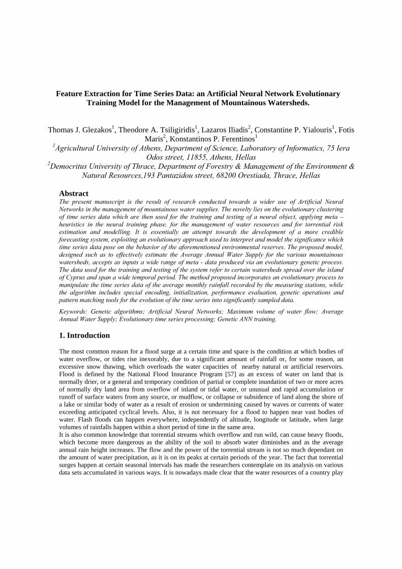
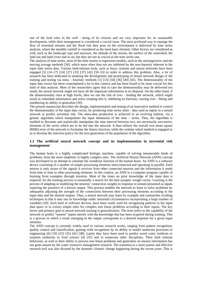
The initial dataset was accumulated out of 78 stations located at the span of the seventy torrential streams. The time span of the initial information covered a period of 28 years, from 1965 to 1993, for most of the stations’ measurements. The current research though, does not average the rainfall time series, but rather takes under consideration the average for every month for each year. The parental research of Iliadis and Maris [22] used three structural input parameters, namely the area of watershed, the altitude and the slope and two dynamic ones, the average annual and the average monthly rain height. For the time span of each dynamic factor, the monthly measurements had been averaged and the result was used as input. The research key point was that it used only two dynamic parameters and among them, only the rain height should be monitored monthly and annually, rendering the acquisition of model inputs effortless and inexpensive both financially and in human resources. The current research differs in that it does not utilize the average annual rain fall at all. Instead, we elected to bring the whole monthly average measurements into play and to search for the best combination of measurements as inputs to the neural network. The key feature of this attempt is that while it keeps the data acquisition at low level of expenses, it also goes to a lower level of input data dimensionality, essentially rendering the input vector more precise. Once trained, the proposed ANN continues to be highly adaptable to various regions and places, provided that the inputs will have been manipulated according to the genetic algorithm decisions. Figure 1 depicts a general view of the island’s mainstreams, while Figure 2 presents the average annual rain height (mm) from 1970 to 2000. Table 1 on the other hand presents a small indicative sample of the data accumulated. All the measurement stations along with the data which they have collected for the whole

time span of the research, belong to the Ministry of Agriculture Natural Resources and Environment of Cyprus [28].

40 Km20

Scale

0

No data available - Area under Turkish occupation

Ammochostos

Larnaka

Keryneia

Lefkosia

Lemesos

Pafos

Polis

800 - 1000

Mean Annual Precipitation (mm)

200 - 400

600 - 800

400 - 600

> 1000

Figure 2. Average annual rain height (mm) from 1970 to 2000. The input data consist of factors which, according to their type, may effectively be classified into two categories, namely structural data in the sense that they remain constant variables for the whole time span of the research, as opposed to dynamic data, category which holds ever changing variables.

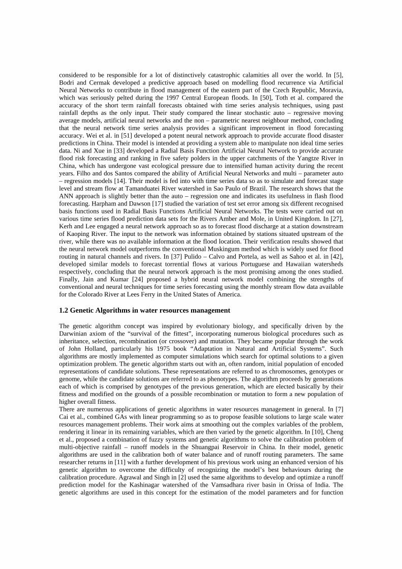
Table 1. Sample of the gathered data M1 – M12: the months of the year, Fn: Area of Watershed, Qmax: Maximum supply, P: Average annual Rainfall, H: Absolute altitude, Jk: Absolute slope, Qmy: Average Annual Water Supply. Station 1 Station 2 Station 3

Year 1965-66 1965-66 1979-80 M1 229 201 195

M2 62 67 165 M3 89 77 135 M4 13 8 25 M5 4 4 9

M6 0 0 0

M7 0 0 0

M8 0 1 5 M9 70 54 1

M10 146 102 60 M11 23 19 133

M12 143 146 169 Fn

(km2) 38 110 22Qmax 54 120 8.6

P(mm) 770 660 810H (m) 550 8 600

Jk (%) 4.2 2.2 8Qmy

(m3/s) 420.62 611.95 330.6

In this context we accumulated a range of 1411 records covering the aforementioned period of time. It was essential for our code to remove any record which had missing values in one or more of the studied factors, so this procedure left us with 1273 patterns of data (inputs and outputs together). This initial recordset was used for the formulation of the training and the testing data sets, comprising of 1152 and 121 patterns respectively. The inputs to the system were the area of the watershed (in km2), the absolute altitude (in

meters), the absolute slope (in percentage) as structural input data, whereas the dynamic input data consisted of the maximum water supply, the average annual rainfall, as well as the average rainfall for each month, for each year of measurement. The network had only one output, the Average Annual Water Supply (in m3/s)

3.2 The Python Programming Language and the Fast Artificial Neural Network Library (FANN)

The research team chose to develop code with the programming language of Python. This selection was two-fold propulsed: on one hand to gain insight in one of the most rapidly developing and integrated computer programming languages available today and, on the other, to use freely distributable open source products. Python, as proved out to be, is easy, powerful and incorporates efficient high level data structures as well as a simple and effective approach to object oriented programming. Being a multi platform language, it allows for programs to be developed on most of the platforms available today. Our source code was writen in Ubuntu Linux, but can be run on a windows – based system just as easily. Python is an interpeted language. This, of course, renders it slower than any compiled language, but the robust approach it offers more than compensates for it. Being an open source project, Python is supported by a vast number of freely available libraries, in addition to the extensive embedded library of its own. Furthermore, the interpreter is easily extended with new functions and data types implemented in C or C++, standard objects and/or modules. Python, is supported by a vast number of freely distributed libraries. One of these is the Fast Artificial Neural Network library (FANN), a free open source neural network library implementing multilayer artificial neural networks in C, with support for both fully connected and sparsely connected networks. Cross-platform execution in both fixed and floating point types are supported, while it also includes a framework for easy handling of training data sets. The FANN library was used so as to construct the neural network module of the application. The evolutionary process was coded in Python from scratch, deriving invaluable assistance from the work presented in [29] by Wonjae Lee and Hak-Young Kim, while the neural network was embedded into it, in order to provide the fitness for the population in each generation and to contribute in the selection of the fittest chromosome.

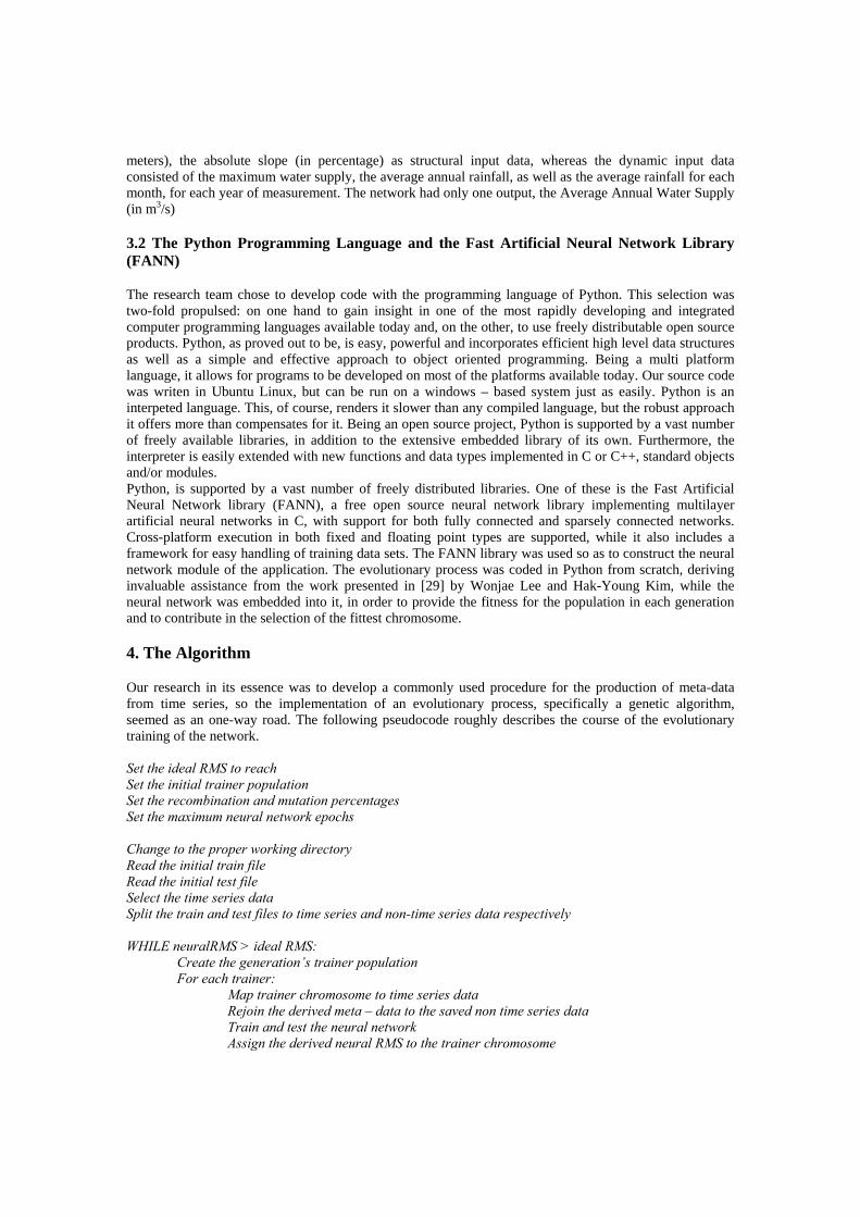
4. The Algorithm

Our research in its essence was to develop a commonly used procedure for the production of meta-data from time series, so the implementation of an evolutionary process, specifically a genetic algorithm, seemed as an one-way road. The following pseudocode roughly describes the course of the evolutionary training of the network. Set the ideal RMS to reach Set the initial trainer population Set the recombination and mutation percentages Set the maximum neural network epochs Change to the proper working directory Read the initial train file Read the initial test file Select the time series data Split the train and test files to time series and non-time series data respectively WHILE neuralRMS > ideal RMS:

Create the generation’s trainer population For each trainer: Map trainer chromosome to time series data Rejoin the derived meta – data to the saved non time series data Train and test the neural network Assign the derived neural RMS to the trainer chromosome

Select trainers according to their fitness for the next generation Apply recombination and mutation procedures to the selected trainer chromosomes

The developed algorithm should be able to produce an initially random population of ‘trainers’ in its initial generation, that is chromosomes behaving in a certain varied predefined manner and able to appropriately manipulate the initial raw time series. The products of the trainers also should be assigned a ‘fitness’ score, that is a floating point value from some function quantifying their relevance towards an optimum solution to the problem. In our case the fitness of each evolutionary produced time series was derived by the root mean square error of the neural network. Thereinafter, the next and subsequent generations of the algorithm were formulated according to a selection policy which should elect the fittest members of the previous generation of the trainers.

4.1 Initial Data Manipulation

The application starts out by incorporating the initial training and testing data set, and then analyzing it in order to create the initial random population of trainer chromosomes. It collects the initial training and testing data and saves them to a locally created nested list, each sublist of which corresponds to one line of the initial raw data time series train and testing files. Consequently, the data is analyzed and the portion of it that corresponds to the initial time series (in our case the twelve values corresponding to the rainfall averages for the months of each year) will be used for the creation of the basic training population of the algorithm (Table 2), while the rest of the initial data, which correspond to the structural and dynamic input non time series data are set aside for future use. The initial generation of the algorithm starts out with a user defined number of training chromosomes, which comprise the basic trainer. Each chromosome of the trainer contains twelve randomly chosen bits in the range of [0, 1], plus two bits in the beginning of the chromosome which stand out as the mechanism bits, driving and manipulating the behavior of the whole chromosome (the bold genes in the trainers of Table 3). So the chromosomes of the trainer for each generation is a binary list of n+2 elements each, where n is the initial time series data (twelve for our case) and the excess pair is the “core mechanism” of the chromosome. The function of the trainer is to essentially “map” its genes to the initial training and testing data sets, according to its mechanism genes. If this is 00 (Table 3, trainer 1), then it stands out as a “Discard-All-Zeros” resampling function. In this case, the time series will be stripped off of its values for which the corresponding genes of the trainer is 0 (table 4, meta-data 1). On the other hand, if it is 11 (Table 3, trainer 2), then it stands out as a “First-One-Last-Zero Average” clustering mechanism for the initial data. In this case, the trainer extracts the everage of the time series elements for every group of its own genes which start with the first 1 and end with the last zero (Table 4, meta-data 2). In the cases where the core mechanism is 01 (Table 3, trainer 3), the chromosome behaves as a “First-One-Last-Zero median” clustering mechanism, which returns the median of the initial data series elements for each cluster which corresponds to the first 1 and the last zero of its own genes (Table 4, meta-data 3). Finally, if the core mechanism is 10 (Table 3, trainer 4), then the chromosome will return the distance of the maximum to the minimum value of every group of the initial time series which is defined in the same aforementioned manner (Table 4, meta-data 4). The following tables depict the mapping of four fictitious trainer – chromosomes of a random generation of the algorithm to some initial raw time series data and the inevitable emergence of four genetically produced meta – data sets.

Table 2

Initial raw time series precipitation data

229 62 89 13 4 1 1 1 70 146 23 143

262 74 101 47 61 5 7 16 9 51 114 120

Table 3 Trainer 1: Resampling discarding zeros 0 0 1 0 0 0 0 1 0 1 0 1 0 1

Trainer 2: First-One-Last-Zero Average 1 1 1 0 0 0 0 1 0 1 0 1 0 1

Trainer 3: First-One-Last-Zero Median 0 1 1 0 0 0 0 1 0 1 0 1 0 1

Trainer 4: First-One-Last-Zero MinMax 1 0 1 0 0 0 0 1 0 1 0 1 0 1 Table 4

Derived meta data

229 1 1 146 143 Meta-data1

262 5 16 51 120

79.4 1.0 35.5 84.5 143 Meta-data2

109.0 6.0 12.5 82.5 120

62.0 1.0 35.5 84.5 143 Meta-data3

74.0 6.0 12.5 82.5 120

225.0 0.0 69.0 123.0 143 Meta-data4

215.0 2.0 7.0 63.0 120

In the above tables, the genome of each trainer corresponding to the twelve months is, for the sake of simplicity, deliberately chosen to be the same (100001010101). The only portion of the genome which varies is the core machine of each chromosome, that is its two starting genes, which dictate the behaviour of thew chromosome. In the case of trainer 1 (00), this will trigger the resampling mechanism of the trainer, discarding each number of the time series which corresponds to its zeros. For the rest of the trainers, each core mechanism will produce essentially five clusters in the time series data, with the corresponding statistical functions, as shown above. It is essential to be cleared at this point that the trainer of the initial generation of the algorithm explicitly contains a chromosome having all of its genes equal to 1, so as to bring forth and test the initial time series unaltered, along with all other tests conducted. Following the mapping of the trainer chromosomes to the time series training and testing data, is the joining phase, in which each “genetically” produced time series training list will again embed the structural and dynamic data from which was initially deprived, in order to be genetically evolved. In the next phase neural training and testing comes into play.

4.2 Neural Training and Testing

In the beginning we confronted the dilemma of constructing a new neural network structure from the ground up, making a variety of testing and trial and error procedures, or to follow the initial research and test the algorithm against the original findings. We chose to proceed with the latter solution, so as to be able to compare the results on more steady grounds. The only alterations which we were unable to avoid were the changing in the input layer of the neural network. That happened because each trainer produces different kind of data of varying inputs, although the output remains unchanged. The code was enhanced with a neural network object from the FANN library, which was used as a landmark for the fitness of the chromosomes. The neural network object was created and trained as a standard backpropagation Multi

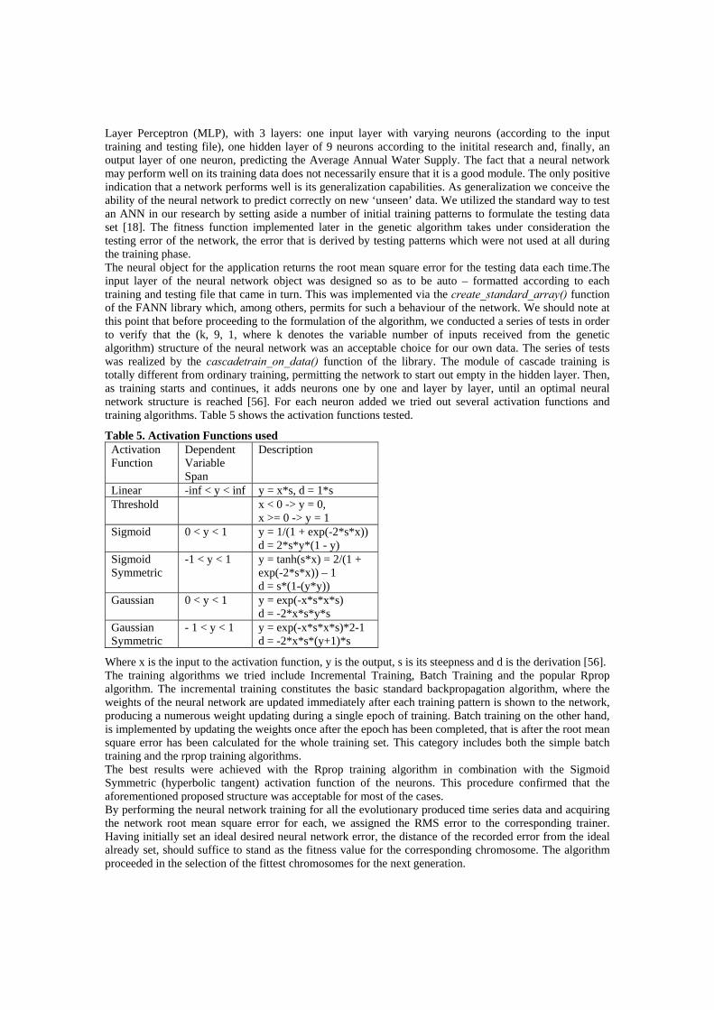
Layer Perceptron (MLP), with 3 layers: one input layer with varying neurons (according to the input training and testing file), one hidden layer of 9 neurons according to the initital research and, finally, an output layer of one neuron, predicting the Average Annual Water Supply. The fact that a neural network may perform well on its training data does not necessarily ensure that it is a good module. The only positive indication that a network performs well is its generalization capabilities. As generalization we conceive the ability of the neural network to predict correctly on new ‘unseen’ data. We utilized the standard way to test an ANN in our research by setting aside a number of initial training patterns to formulate the testing data set [18]. The fitness function implemented later in the genetic algorithm takes under consideration the testing error of the network, the error that is derived by testing patterns which were not used at all during the training phase. The neural object for the application returns the root mean square error for the testing data each time.The input layer of the neural network object was designed so as to be auto – formatted according to each training and testing file that came in turn. This was implemented via the create_standard_array() function of the FANN library which, among others, permits for such a behaviour of the network. We should note at this point that before proceeding to the formulation of the algorithm, we conducted a series of tests in order to verify that the (k, 9, 1, where k denotes the variable number of inputs received from the genetic algorithm) structure of the neural network was an acceptable choice for our own data. The series of tests was realized by the cascadetrain_on_data() function of the library. The module of cascade training is totally different from ordinary training, permitting the network to start out empty in the hidden layer. Then, as training starts and continues, it adds neurons one by one and layer by layer, until an optimal neural network structure is reached [56]. For each neuron added we tried out several activation functions and training algorithms. Table 5 shows the activation functions tested.

Table 5. Activation Functions used Activation Function

Dependent Variable Span

Description

Linear -inf < y < inf y = x*s, d = 1*s Threshold x < 0 -> y = 0,

x >= 0 -> y = 1 Sigmoid 0 < y < 1 y = 1/(1 + exp(-2*s*x))

d = 2*s*y*(1 - y) Sigmoid Symmetric

-1 < y < 1 y = tanh(s*x) = 2/(1 + exp(-2*s*x)) – 1 d = s*(1-(y*y))

Gaussian 0 < y < 1 y = exp(-x*s*x*s) d = -2*x*s*y*s

Gaussian Symmetric

- 1 < y < 1 y = exp(-x*s*x*s)*2-1 d = -2*x*s*(y+1)*s

Where x is the input to the activation function, y is the output, s is its steepness and d is the derivation [56]. The training algorithms we tried include Incremental Training, Batch Training and the popular Rprop algorithm. The incremental training constitutes the basic standard backpropagation algorithm, where the weights of the neural network are updated immediately after each training pattern is shown to the network, producing a numerous weight updating during a single epoch of training. Batch training on the other hand, is implemented by updating the weights once after the epoch has been completed, that is after the root mean square error has been calculated for the whole training set. This category includes both the simple batch training and the rprop training algorithms. The best results were achieved with the Rprop training algorithm in combination with the Sigmoid Symmetric (hyperbolic tangent) activation function of the neurons. This procedure confirmed that the aforementioned proposed structure was acceptable for most of the cases. By performing the neural network training for all the evolutionary produced time series data and acquiring the network root mean square error for each, we assigned the RMS error to the corresponding trainer. Having initially set an ideal desired neural network error, the distance of the recorded error from the ideal already set, should suffice to stand as the fitness value for the corresponding chromosome. The algorithm proceeded in the selection of the fittest chromosomes for the next generation.

4.3 Selection Policy and Intermediate Generation

In order to formulate each next generation of the algorithm, there was a need to create a ‘behind-the-scenes’ intermediate generation at the end of the current generation. This holds the fittest members of the generation, as well as other chromosomes not so fit. The policy of selecting the best offspring incorporated the stochastic procedure known as roulette wheel selection. If f(gi) denotes the fitness function of each of g = Ν individual chromosomes, the chromosome gi, i = 1, 2, …, N has probability

N

ii

i

gf

gf

1

)(

)(

of being selected. The roulette wheel incorporates a fitness proportionate selection operator, which elects to perpetuate the fittest chromosomes, i.e. the ones with the higher fitness score. In this context, chromosomes with relatively high fitness scores are less likely to be eliminated. On the other hand, less fit chromosomes may not be extinguished from the genetic pool of the next generations. This results in the fact that some weaker solutions to the problem at hand may survive the algorithm sweep for the forming of the next generations, conveying their potentially useful genes to their offspring. The roulette wheel algorithm in our case initiates by calculating the sum of the fitnness scores af all the trainer chromosomes assigned to them during the previous steps and then creates a probability list for each one of them by dividing each individual fitness score with the sum of all the scores. In the next step the algorithm creates a cumulative probability list by adding succeeding probability scores to each other. It then constructs a list of selected indexes, the length of which is always 100, by sequentially electing chromosome probability scores by comparing them to a randomly generated number. This list contains the indexes of the selected trainer chromosomes. Figure 3. Schematic depiction of the evolutionary training procedure

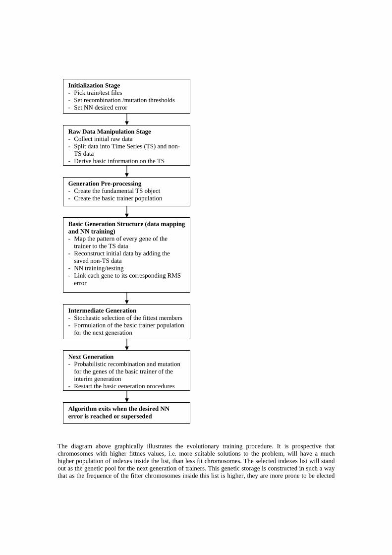
The diagram above graphically illustrates the evolutionary training procedure. It is prospective that chromosomes with higher fittnes values, i.e. more suitable solutions to the problem, will have a much higher population of indexes inside the list, than less fit chromosomes. The selected indexes list will stand out as the genetic pool for the next generation of trainers. This genetic storage is constructed in such a way that as the frequence of the fitter chromosomes inside this list is higher, they are more prone to be elected

Initialization Stage - Pick train/test files - Set recombination /mutation thresholds - Set NN desired error

Raw Data Manipulation Stage - Collect initial raw data - Split data into Time Series (TS) and non-

TS data - Derive basic information on the TS

Generation Pre-processing - Create the fundamental TS object - Create the basic trainer population

Basic Generation Structure (data mapping and NN training) - Map the pattern of every gene of the

trainer to the TS data - Reconstruct initial data by adding the

saved non-TS data - NN training/testing - Link each gene to its corresponding RMS

error

Intermediate Generation - Stochastic selection of the fittest members - Formulation of the basic trainer population

for the next generation

Next Generation - Probabilistic recombination and mutation

for the genes of the basic trainer of the interim generation

- Restart the basic generation procedures

Algorithm exits when the desired NN error is reached or superseded

as parents fo the next generation, without forbidding the selection of less fit chromosomes, of course with a much lower probability. 4.4 Formulation of the Next Generation

At the stage when the population of the intermediate generation is fixed, the genetic mechanisms of the algorithm formulate the next generation. For each randomly picked pair of chromosomes of the intermediate generation there is an arbitrary set probability of selection, recombination or mutation. Recombination of chromosomes is the procedure in which the parents contribute with different supplementary parts of their genome in the production of their offspring. In our algorithm, the ‘breaking point’ for the chromosome of the parent is random within the bounds of each parent genome. On the other hand, mutation refers to the ‘flipping’ of an offspring’s random gene. It is well known and well documented in the literature that a proper amount of time should be invested in the fine tuning of the mutation and recombination probability of the genetic algorithm. An excessively small mutation rate may lead to “genetic drift”, that is the statistical effect that stems from the influence that probability poses on the survival of alleles (variants of a gene, 0 or 1 in our case) and the trait that it confers to the chromosome. A positive genetic drift renders the allele paramount in the genetic pool, whereas a negative genetic drift may extinct the allele. Both limits, either too high, or too low, in the genetic drift could potentially pose irreparable damage to the genetic pool, lowering variability to unacceptable levels [38] [43] [44]. The same holds true for the recombination probability. A variety of recombination and mutation probabilities were tested, concluding on selecting 0.4 and 0.005 respectively.

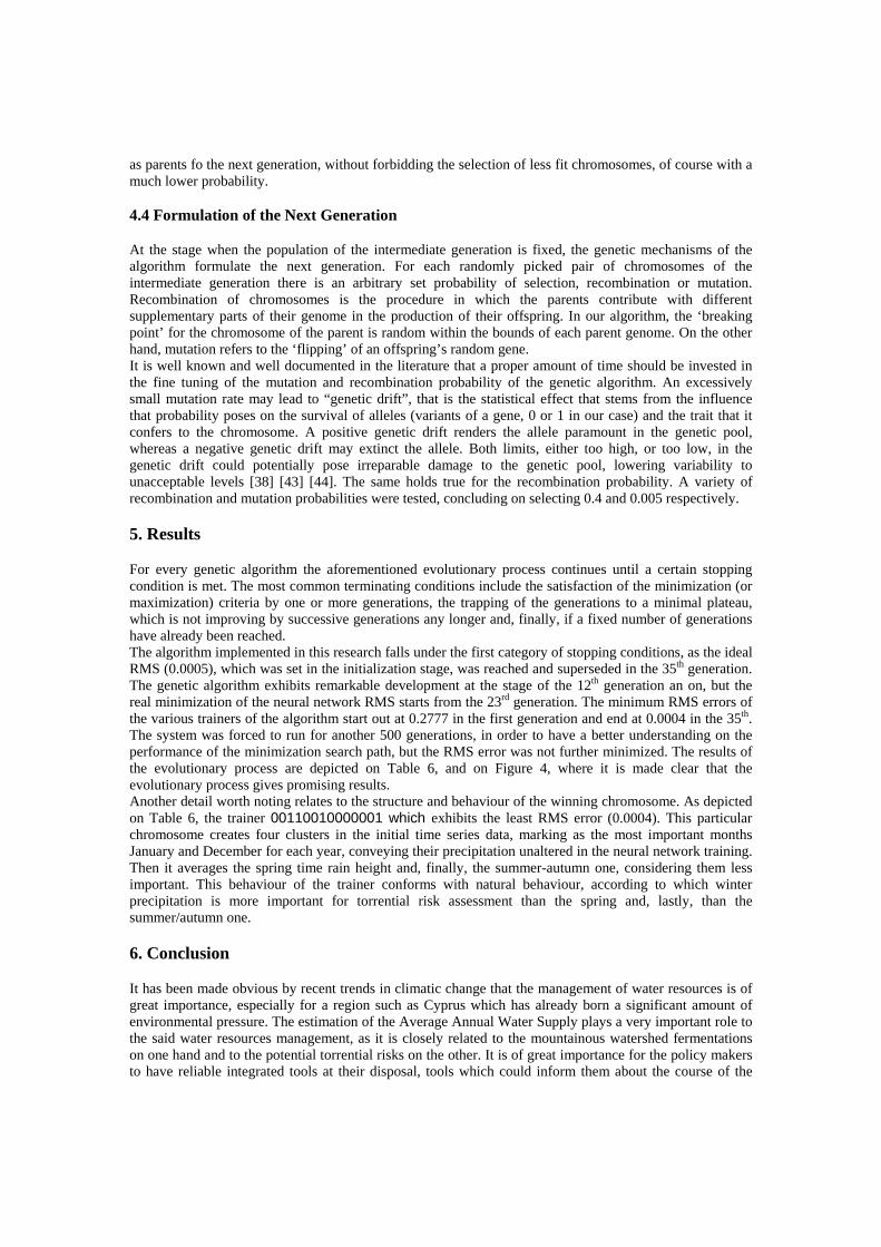
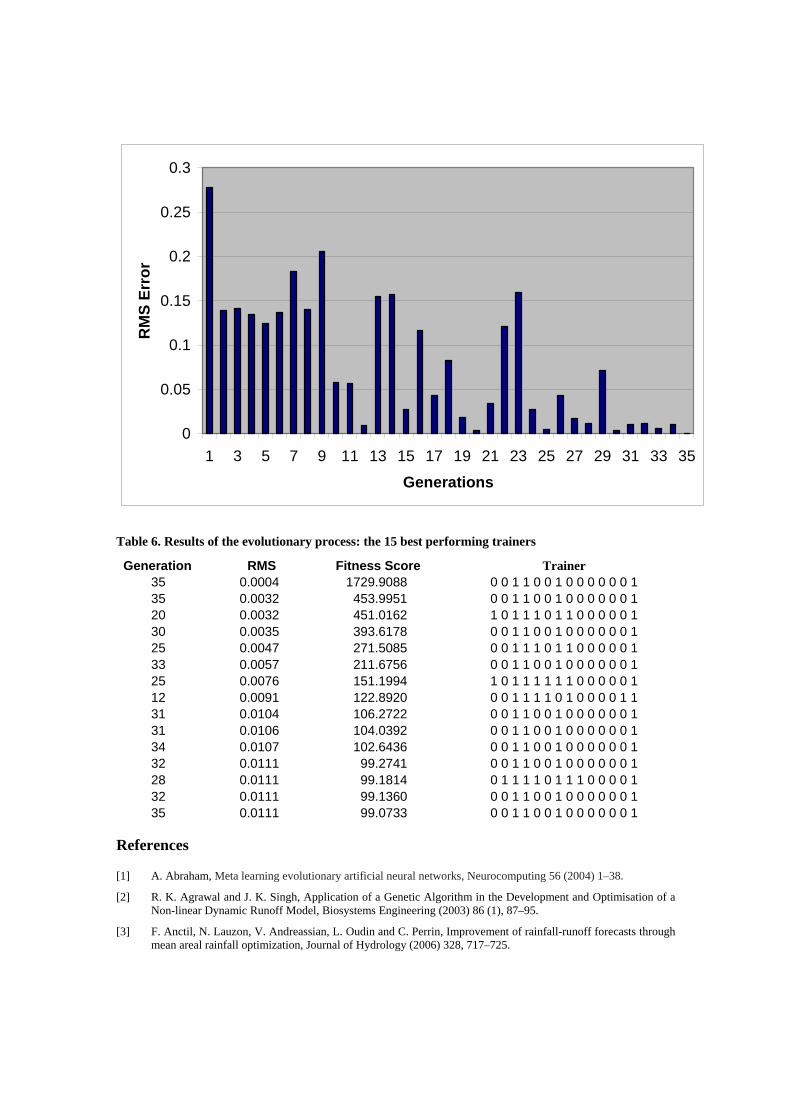
5. Results

For every genetic algorithm the aforementioned evolutionary process continues until a certain stopping condition is met. The most common terminating conditions include the satisfaction of the minimization (or maximization) criteria by one or more generations, the trapping of the generations to a minimal plateau, which is not improving by successive generations any longer and, finally, if a fixed number of generations have already been reached. The algorithm implemented in this research falls under the first category of stopping conditions, as the ideal RMS (0.0005), which was set in the initialization stage, was reached and superseded in the 35th generation. The genetic algorithm exhibits remarkable development at the stage of the 12th generation an on, but the real minimization of the neural network RMS starts from the 23rd generation. The minimum RMS errors of the various trainers of the algorithm start out at 0.2777 in the first generation and end at 0.0004 in the 35th. The system was forced to run for another 500 generations, in order to have a better understanding on the performance of the minimization search path, but the RMS error was not further minimized. The results of the evolutionary process are depicted on Table 6, and on Figure 4, where it is made clear that the evolutionary process gives promising results. Another detail worth noting relates to the structure and behaviour of the winning chromosome. As depicted on Table 6, the trainer 00110010000001 which exhibits the least RMS error (0.0004). This particular chromosome creates four clusters in the initial time series data, marking as the most important months January and December for each year, conveying their precipitation unaltered in the neural network training. Then it averages the spring time rain height and, finally, the summer-autumn one, considering them less important. This behaviour of the trainer conforms with natural behaviour, according to which winter precipitation is more important for torrential risk assessment than the spring and, lastly, than the summer/autumn one.

6. Conclusion

It has been made obvious by recent trends in climatic change that the management of water resources is of great importance, especially for a region such as Cyprus which has already born a significant amount of environmental pressure. The estimation of the Average Annual Water Supply plays a very important role to the said water resources management, as it is closely related to the mountainous watershed fermentations on one hand and to the potential torrential risks on the other. It is of great importance for the policy makers to have reliable integrated tools at their disposal, tools which could inform them about the course of the

phenomena in the near future. It is also of great importance that these tools requirements are kept at as lower cost as possible, both at the financial level and at the human-day occupation. The main advantage of the present research work, as well as its parental one, is the fact that it proposes the development of a tool for the prediction of a key factor in water management and torrential risk and elimination, which requires minimal effort and expense as it measures only two dynamic input factors. Obviously, the structural input data are not to change for the relatively small era of measurements that are conducted, thus the only factor which is to be monitored as precisely as possible on a daily basis is rain - height. Furthermore, the developed module can be re-adjusted and developed by continuous training, as new input data flow in and, provided the availability of training data could be proposed for different regions. The crucial contribution of the present research work is the evolutionary clustering and re-sampling of the initial time series data. The advantages of the proposed approach are numerous. Firstly, the researcher and the developer of the system has a vast number of training / testing data at his disposal, because now we do not need to average the whole time span of measurements of the monthly rain height and create only one record of input patterns. Instead, every year has become an input pattern for our system, effectively multiplying the number of the initial data set. Also, the evolutionary process diminishes both the total number of inputs, as well as the potential noise inherent in the input time series data. This way we have succeeded in effectively train the proposed neural network and produce reliable estimations, while keeping the operating costs at acceptable levels. There is always, of course, the invariable dilemma of the representation of the gene. In our case, we have conducted a number of training scenarios some of which included the floating point representation of the basic trainer genes, instead of the binary one. This configuration though posed a lot of problems and was eventually dropped. For one, the whole system was very demanding in computing power, partly due to the requirements posed by the programming language, as well as the structure of the initial row data itself. The system also crashed in certain circumstances, when the algorithm produced illegal gene values or even illegal clustering configurations in the time series. Although these obstacles were too important to be overlooked, the benefits committed by a floating point representation of the gene, such as greater variability among the offspring and increased probability for the algorithm to overcome trapping in luring local minima, has posed a challenging prospect for the future. The plans of the research team is to essentially widen the scope of the algorithm, along with its potential, by adding more machine genes at the chromosomes of the generation trainers, so as to force them to expand their search plane. This development may probably require the re-engineering of the core code of the program so as to keep its computational demands at as low a level as possible. Also, the development of a Graphical User Interface (GUI), which could render the application friendlier to the average user, could contribute to the acceptance of the software in different regions.

Figure 4. The course of the evolutionary process

0

0.05

0.1

0.15

0.2

0.25

0.3

1 3 5 7 9 11 13 15 17 19 21 23 25 27 29 31 33 35

Generations

RM

S E

rro

r

Table 6. Results of the evolutionary process: the 15 best performing trainers

Generation RMS Fitness Score Trainer 35 0.0004 1729.9088 0 0 1 1 0 0 1 0 0 0 0 0 0 1 35 0.0032 453.9951 0 0 1 1 0 0 1 0 0 0 0 0 0 1 20 0.0032 451.0162 1 0 1 1 1 0 1 1 0 0 0 0 0 1 30 0.0035 393.6178 0 0 1 1 0 0 1 0 0 0 0 0 0 1 25 0.0047 271.5085 0 0 1 1 1 0 1 1 0 0 0 0 0 1 33 0.0057 211.6756 0 0 1 1 0 0 1 0 0 0 0 0 0 1 25 0.0076 151.1994 1 0 1 1 1 1 1 1 0 0 0 0 0 1 12 0.0091 122.8920 0 0 1 1 1 1 0 1 0 0 0 0 1 1 31 0.0104 106.2722 0 0 1 1 0 0 1 0 0 0 0 0 0 1 31 0.0106 104.0392 0 0 1 1 0 0 1 0 0 0 0 0 0 1 34 0.0107 102.6436 0 0 1 1 0 0 1 0 0 0 0 0 0 1 32 0.0111 99.2741 0 0 1 1 0 0 1 0 0 0 0 0 0 1 28 0.0111 99.1814 0 1 1 1 1 0 1 1 1 0 0 0 0 1 32 0.0111 99.1360 0 0 1 1 0 0 1 0 0 0 0 0 0 1 35 0.0111 99.0733 0 0 1 1 0 0 1 0 0 0 0 0 0 1

References

[1] A. Abraham, Meta learning evolutionary artificial neural networks, Neurocomputing 56 (2004) 1–38.

[2] R. K. Agrawal and J. K. Singh, Application of a Genetic Algorithm in the Development and Optimisation of a Non-linear Dynamic Runoff Model, Biosystems Engineering (2003) 86 (1), 87–95.

[3] F. Anctil, N. Lauzon, V. Andreassian, L. Oudin and C. Perrin, Improvement of rainfall-runoff forecasts through mean areal rainfall optimization, Journal of Hydrology (2006) 328, 717–725.

[4] S. Avramidis and L. Iliadis, Wood-Water Isotherm Prediction with Artificial Neural Networks: a Preliminary Study Holzforschung, ISSN: 0018-3830 59 (3), 336-341. Berlin, New York, Walter De Gruyter & Co.

[5] L. Bodri and V. Cermak, Prediction of extreme precipitation using a neural network: application to summer flood occurrence in Moravia, Advances in Engineering Software 31 (2000) 311–321.

[6] L. Boillereaux, C. Cadet and A. Le Bail, Thermal properties estimation during thawing via real time neural network learning, J. Food Eng. 57(1) (2003) 17-23.

[7] X. Cai, D. C. McKinney and L. S. Lasdon, Solving nonlinear water management models using a combined genetic algorithm and linear programming approach, Advances in Water Resources 24 (2001) 667–676.

[8] C. L. Chang, S. L. Lo and S. L. Yu, Applying fuzzy theory and genetic algorithm to interpolate precipitation, Journal of Hydrology 314 (2005) 92–104.

[9] K. W. Chau, A split-step particle swarm optimization algorithm in river stage forecasting, Journal of Hydrology 346 (2007), 131–135.

[10] C. T. Cheng, C. P. Ou and K. W. Chau, Combining a fuzzy optimal model with a genetic algorithm to solve multi-objective rainfall – runoff model calibration, Journal of Hydrology 268 (2002) 72–86.

[11] Cheng, C. T., Zhao, M. Y., Chau, K. W. and X. Y. Wu, 2006. Using genetic algorithm and TOPSIS for Xinanjiang model calibration with a single procedure. Journal of Hydrology 316 (2006) 129–140.

[12] C. Damle and A. Yalcin, Flood prediction using Time Series Data Mining, Journal of Hydrology 333 (2007), 305–316.

[13] D. A. Elizondo, R. Birkenhead, M. Gongora, E. Taillard and P. Luyima, Analysis and test of efficient methods for building recursive deterministic perceptron neural networks, Neural Networks 20 (2007) 1095–1108.

[14] A. J. P. Filho and C. C. dos Santos, Modeling a densely urbanized watershed with an artificial neural network, weather radar and telemetric data, Journal of Hydrology 317 (2006) 31–48.

[15] P. J. Gallant and G. J. M. Aitken, Genetic algorithm design of complexity-controlled time-series predictors, 0-7803-8178-5/03, IEEE XIII Workshop on Neural Networks for Signal Processing.

[16] J. V. Hansen, J. B. McDonald and R. D. Nelson, Time series prediction with genetic algorithm designed neural networks: an Empirical comparison with modern statistical models, Computational Intelligence, 15(3) (1999).

[17] C. Harpham and C. W. Dawson, The effect of different basis functions on a radial basis function network for time series prediction: A comparative study, Neurocomputing 69 (2006) 2161–2170.

[18] S. Haykin, Neural Networks, A Comprehensive Foundation (Prentice Hall International, New Jersey, 1989).

[19] M. A. Hussain, M. S. Rahman and C.W. Ng. Prediction of pores formation (porosity) in foods during drying: generic models by the use of hybrid neural network. J. Food Eng. 51 (2002) 239-248.

[20] Igel

[21] L. Iliadis and F. Maris, An Artificial Neural Network to estimate average maximum instant water – flow of watersheds, in: Proceedings of the ninth International Conference of Engineering Applications of Neural Networks, Lille, France (2005) 215–222.

[22] L. Iliadis and F. Maris, An Artificial Neural Network model for mountainous water-resources management. The case of Cyprus mountainous watersheds, Environmental Modelling and Software (2006) 1-7.

[23] L. Iliadis and S. Spartalis, Fundamental Fuzzy Relation Concepts of a D.S.S. for the Estimation of Natural Disasters’ Risk (The case of a trapezoidal membership function), Mathematical and Computer Modelling 42 (2005) 747-758.

[24] A. Jain and A. M. Kumar, Hybrid neural network models for hydrologic time series forecasting, Applied Soft Computing 7 (2007) 585–592.

[25] Jambunathan K., Hartle S.L., Ashforth-Frost S. and V.N. Fontana, 1996. Evaluating convective heat transfer coefficients using neural networks. Int. J. Heat Mass Transfer 39(11):2329-2332.

[26] R. Kerachian and M. Karamouz, A stochastic conflict resolution model for water quality management in reservoir – river systems. Advances in Water Resources 30 (2007) 866–882

[27] T. Kerh, and C. S. Lee, Neural networks forecasting of flood discharge at an unmeasured station using river upstream information. Advances in Engineering Software 37 (2006) 533–543.

[28] D. Kyprhs and P. Neofytou, Monthly River Supplies of Cyprus, Monthly Rain-Falls, Maximums of instant flow, Ministry of Agriculture Natural Resources and Environment, Department of Water Development, Cyprus.

[29] W. Lee and H. Y. Kim, Genetic algorithm implementation in Python, Fourth Annual ACIS International Conference on Computer and Information Science (ICIS’05), ISBN: 0-7695-2296-3, Digital Object Identifier 10.1109/ICIS.2005.69, 2005, pp.8–11

[30] F. Liu, G. S. Ng and C. Quek, RLDDE: A novel reinforcement learning-based dimension and delay estimator for neural networks in time series prediction. Neurocomputing 70 (2007) 1331-1341

[31] Mahfoud,

[32] R. M. Myhara and S. Sablani, Unification of food water sorption isotherms using artificial neural networks. Drying Technol. 19(8) (2001) 1543-1554.

[33] J. R. Ni and A. Xue, Application of artificial neural network to the rapid feed back of potential ecological risk in flood diversion zone, Engineering Applications of Artificial Intelligence 16 (2003) 105–119.

[34] H. Niska, T. Hiltunen, A. Karppinen, J. Ruuskanen and M. Kolehmainen, Evolving the neural network model for forecasting air pollution time series, Engineering Applications of Artificial Intelligence 17 (2004) 159–167.

[35] J. Paliwal, N. S. Visen and D. S. Jayas, Evaluation of neural network architectures for cereal grain classification using morphological features, J. Agri. Eng. 79(4) (2001) 361-370.

[36] R. B. C. Prudencio, and T. B. Ludermir, Meta-learning approaches to selecting time series models, Neurocomputing 61 (2004) 121 – 137.

[37] L. Pulido – Calvo, and M. M. Portela, Application of neural approaches to one-step daily flow forecasting in Portuguese watersheds, Journal of Hydrology (2007) 332, 1– 15.

[38] L. Qing, W. Gang, Y. Zaiyue, and W. Qiuping, Crowding clustering genetic algorithm for multimodal function optimization, Applied Soft Computing 8 (2006) 88–95.

[39] Riedmiller

[40] F. Rossi, N. Delannay, B. Conan-Guez and M. Verleysen, Representation of functional data in neural networks, Neurocomputing 64 (2005) 183–210,

[41] S. S. Sablani, O.D. Baik and M. Marcotte, Neural networks for predicting thermal conductivity of bakery products. J. Food Eng. 52 (2002) 299-304.

[42] G. B. Sahoo, C. Ray and E. H. De Carlo, Use of neural network to predict flash flood and attendant water qualities of a mountainous stream on Oahu, Hawaii, Journal of Hydrology (2006) 327, 525– 538.

[43] L. M. Schmitt, Fundamental Study. Theory of genetic algorithms, Theoretical Computer Science 259 (2001) 1-61.

[44] L. M. Schmitt, Theory of Genetic Algorithms II: models for genetic operators over the string-tensor representation of populations and convergence to global optima for arbitrary fitness function under scaling, Theoretical Computer Science 310 (2004) 181 – 231.

[45] R. K. Sivagaminathan and S. Ramakrishnan, A hybrid approach for feature subset selection using neural networks and ant colony optimization, Expert Systems with Applications 33 (2007) 49–60

[46] S. Spartalis, L. Iliadis and F. Maris, An Innovative Risk evaluation System estimating its own Fuzzy Entropy, Mathematical and Computer Modelling 46, Issues1-2 (2007) 260-267.

[47] S. Spartalis, L. Iliadis, F. Maris and D. Marinos, A Decision Support System Unifying Fuzzy Trapezoidal Function Membership Values Using T-Norms: The case of river Evros Torrential Risk Estimation, ICNAAM2004 Intern. Conf. on Numerical Analysis and Applied Mathematics WILEY-VCH Verlag GmbH & Co. KGaA, ISBN 3-527-40563-1, (2004) 173-176.

[48] S. Sreekanth, H. S. Ramaswamy and S.S. Sablani, Prediction of psychrometric parameters using neural networks, Drying Technol. 16(3-5) (1998) 825.

[49] S. Srinivasulu and A. Jain, A comparative analysis of training methods for artificial neural network rainfall – runoff models, Applied Soft Computing 6 (2006) 295–306.

[50] E. Toth, A. Brath and A. Montanari, Comparison of short-term rainfall prediction models for real-time flood forecasting. Journal of Hydrology 239 (2000) 132–147.

[51] Y. Wei, W. Xu, Y. Fan and H. T. Tasi, Artificial neural network based predictive method for flood disaster, Computers and Industrial Engineering 42 (2002) 383–390.

[52] R. N. Yadav, P. K. Kalra and J. John, Time series prediction with single multiplicative neuron model, Applied Soft Computing 7 (2007) 1157–1163.

[53] P. C. Young, Advances in real-time flood forecasting, Philosophical Transactions of the Royal Society London. A 360 (2002) 1433-1450

References on the World Wide Web

[54] Cyprus Broadcasting Corporation. http://www.hri.org/news/cyprus/riken/

[55] Cyprus Government, http://www.moi.gov.cy

[56] Fast Artificial Neural Network Library (FANN), http://leenissen.dk/fann

[57] National Flood Insurance Program, http://www.floodsmart.gov

Must Download:

1. Mahfoud, S. W., 1994. Crossover interactions among niches. IEEE, http:// www.ieee.org

2. Riedmiller, M. and Braun, 1993. H.: A direct adaptive method for faster backpropagation learning: the RPROP algorithm, Proc. Int. Conference on Neural Networks, San Franscisco, CA, 1 (1993) 586-591.

3. C. Igel, M. Hüsken, Improving the Rprop learning algorithm, in: Proceedings of the Second International ICSC Symposium on Neural Computation (NC 2000), ICSC Academic Press, Canada/Switzerland, 2000, pp. 115–121.