feature selection for appearance-based vehicle...

Feature Selection for Appearance-based Vehicle Tracking inGeospatial Video

Mahdieh Poostchia Filiz Bunyaka Kannappan Palaniappana Guna Seetharamanb

aDepartment of Computer Science, University of Missouri-ColumbiabAir Force Research Laboratory, Rome, NY, USA

ABSTRACT

Current video tracking systems often employ a rich set of intensity, edge, texture, shape and object level featurescombined with descriptors for appearance modeling. This approach increases tracker robustness but is compu-tationally expensive for realtime applications and localization accuracy can be adversely affected by includingdistracting features in the feature fusion or object classification processes. This paper explores offline featuresubset selection using a filter-based evaluation approach for video tracking to reduce the dimensionality of thefeature space and to discover relevant representative lower dimensional subspaces for online tracking. We com-pare the performance of the exhaustive FOCUS algorithm to the sequential heuristic SFFS, SFS and RELIEFfeature selection methods. Experiments show that using offline feature selection reduces computational complex-ity, improves feature fusion and is expected to translate into better online tracking performance. Overall SFFSand SFS perform very well, close to the optimum determined by FOCUS, but RELIEF does not work as well forfeature selection in the context of appearance-based object tracking.

Keywords: Feature Selection, Object Tracking, SFFS, SFS, FOCUS, RELIEF, Geospatial Video

1. INTRODUCTION

Object tracking in video requires robustness to imaging conditions, environmental characteristics, sensor responseand appearance variability. Current video tracking systems often employ a rich set of intensity, edge, texture,shape and object level features combined with descriptors for appearance modeling.1–11 These descriptors areused in conjunction with other cues such as motion, object class, and background clutter to detect and tracktargets over time. This approach increases tracker robustness but is computationally expensive for realtimeapplications and localization accuracy can be affected by including lower quality features in the feature fusion orobject classification processes. This paper explores offline feature subset selection for video tracking to reduce thedimensionality of the feature space and to discover a representative lower dimensional (non-projection) subspacefor online tracking. Optimal feature subset selection is combinatorially intractable when the feature space islarge. We compare the complete FOCUS12 to the dynamic sequential floating forward search (SFFS),13 thegreedy sequential forward selection (SFS)14 and the instance learning based RELIEF15 models - four standardapproaches used in machine learning. Given an application specific evaluation function, the FOCUS algorithmexhaustively explores the best feature combination, while the SFFS algorithm sequentially finds the local bestfeature subset by considering the conditional inclusion and exclusion of the features. The SFS is a greedyalgorithm and may fail to select the optimal solution. The RELIEF algorithm doesn’t directly select the bestfeatures but rather gives each feature a weight indicating its level of relevance to the class label.

Our feature subset evaluation system is independent of the full tracking environment and uses just the groundtruth target locations. We developed a separate test-bed for filtering-based feature selection in order to decouplefeature performance from the rest of the tracking system where the final outcome depends not only on the featuresused but also on the other parameters like the predictor performance and target kinematics. Likelihood maps foreach feature are constructed using sliding window comparison between the target and a region of interest (ROI).Local maxima in each feature likelihood map are sorted based on their peak strengths (match likelihoods). Thepeak rank/order of the local maxima corresponding to the target location is used to quantify the performanceof the feature producing the likelihood map. Several likelihood fusion methods can be used to combine multiplefeature likelihood maps into a single joint likelihood map at each iteration. Each of the feature sets is evaluatedover all the targets and frames to obtain an aggregate score. All four feature selection algorithms used in this

Geospatial InfoFusion III, edited by Matthew F. Pellechia, Richard J. Sorensen,Kannappan Palaniappan, Proc. of SPIE Vol. 8747, 87470G · © 2013 SPIE

CCC code: 0277-786X/13/$18 · doi: 10.1117/12.2015672

Proc. of SPIE Vol. 8747 87470G-1

Downloaded From: http://proceedings.spiedigitallibrary.org/ on 06/17/2013 Terms of Use: http://spiedl.org/terms

paper are evaluated under the same conditions. FOCUS which is not practical for larger feature sets becauseof its exhaustive search, is feasible in this study and produces the best results. The SFFS-based selection hasperformance similar to greedy SFS selection and both outperform the RELIEF method for the vehicle trackingapplication. The linear RELIEF unlike the other feature selection methods which produce the same results eachtime, uses random class sampling so the resulting weights change from run to run.

Experiments show that using offline feature selection reduces computational complexity, improves featurefusion that can in turn lead to better online tracking performance. Overall SFFS and SFS perform very well,close to the optimum determined by FOCUS, but RELIEF does not work as well for feature selection in thecontext of appearance-based object tracking. Section 2 presents a short review of our interactive low framerate Likelihood of Features Tracking (LoFT) system. Section 3 describes the four well-known feature selectionalgorithms used in this study. Section 4 describes the evaluation testbed followed by experimental results andconclusions.

2. FEATURE SET FOR APPEARANCE-BASED VEHICLE TRACKING IN WAMI

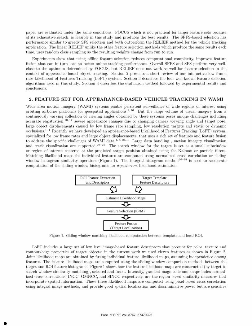
Wide area motion imagery (WAMI) systems enable persistent surveillance of wide regions of interest usingorbiting airborne platforms for geospatial applications.2,16 But the large volume of visual imagery from acontinuously varying collection of viewing angles obtained by these systems poses unique challenges includingaccurate registration,10,17 severe appearance changes due to changing camera viewing angle and target pose,large object displacements caused by low frame rate sampling, low resolution targets and static or dynamicocclusions.1–4 Recently we have developed an appearance-based Likelihood of Features Tracking (LoFT) system,specialized for low frame rates and large object displacements, that uses a rich set of features and feature fusionto address the specific challenges of WAMI data.1,3, 18,19 Large data handling , motion imagery visualizationand track visualization are supported.20–25 The search window for the target is set as a small subwindowor region of interest centered at the predicted target position obtained using the Kalman or particle filters.Matching likelihood maps for individual features are computed using normalized cross correlation or slidingwindow histogram similarity operators (Figure 1). The integral histogram method26–28 is used to acceleratecomputation of the sliding window histograms for a posteriori likelihood estimation.

ROI Feature Extraction

and Descriptors

Target Template

Feature Descriptors

Estimate Likelihood Maps

Feature Selection (K<M)

Feature Fusion

(Target Localization)

Figure 1. Sliding window matching likelihood computation between template and local ROI.

LoFT includes a large set of low level image-based feature descriptors that account for color, texture andcontour/edge properties of target objects; in the current work we used eleven features as shown in Figure 2.Joint likelihood maps are obtained by fusing individual feature likelihood maps, assuming independence amongfeatures. The feature likelihood maps are computed using the sliding window comparison methods between thetarget and ROI feature histograms. Figure 1 shows how the feature likelihood maps are constructed (by target tosearch window similarity matching), selected and fused. Intensity, gradient magnitude and shape index normal-ized cross-correlations, INCC, GMNCC, and SINCC respectively, are the region-based similarity measures thatincorporate spatial information. These three likelihood maps are computed using pixel-based cross correlationusing integral image methods, and provide good spatial localization and discriminative power but are sensitive



to changes in pose, viewing angle and scale. Histogram-based descriptors on the other hand provide global infor-mation about an object that can be robust to changes due to motion, pose, or viewing angle using appropriatenormalization and alignment operations. Gradient histograms further increase this robustness with decreasedsensitivity to illumination change. LoFT uses six histogram based features including three gradient-based (firstderivative) operators (HMG, HOG, HARST) and three Hessian matrix-based (second derivative) operators (HSI,HNCI, HEO) as shown in Figure 2. The adaptive robust structure tensor (ARST) operator provides more ac-curate local orientation estimation in the presence of noise.29 The shape index and the normalized curvatureindex are derived from the eigenvalues of the Hessian matrix. The magnitude weighted histogram of the Hessianeigenvector orientations are used to compute local shape-based features. In addition to these feature descriptorstwo additional descriptors are used – intensity histogram (HI) to represent intensity/color information, and thelocal binary pattern (HLBP) histogram to capture statistical and structural properties of object texture.

Each of the feature maps is binned into ten categories except for HLBP. LoFT uses the uniform rotation-invariant LBP consisting of 18 pattern classes.1,3, 30 The dimensionality of the feature space for feature selectioncan be interpreted in several different ways – if the output of each feature operator is treated as a feature vectorand we concatenate pixel level information within the car template model window then the dimensionality of thefeature space would be 13, 475 for a template model window size of 35×35 pixels. On the other hand if the pixellevel information is aggregated into region statistics and we concatenate the histogram bins together then thedimensionality of the feature space will be only 118. If we use the feature likelihood maps after histogram-basedmatching then the dimensionality will be just 11. In this paper we use the last case in order to be able to compareresults with the exhaustive enumeration approach (i.e. FOCUS) which finds the optimal feature subset. Notethe combinatorial enumeration using FOCUS for feature subset selection is not possible for the other two casessince the feature space dimensionality is too large.

Intensity histogram

Intensity normalized cross correlation

Gradient Magnitude

Gradient Orientation

ARST Orientation

Gradient Magnitude normalized cross correlation

Shape Index

Normalized Curvature Index

Hessian eigenvector orientations

Shape Index correlation

LBP

Candidate Feature Set

Feature

Label

Feature

Number H/C

HI

INCC

HMG

HOG

HARST

GMNCC

HSI

HNCI

HEO

SINCC

HLBP

1

8

2

6

10

9

3

4

5

11

7

H

C

H

H

H

C

H

H

H

C

H

Figure 2. Visual appearance-based feature descriptors used in LoFT for object tracking in WAMI.1,3

3. BRIEF OVERVIEW OF SELECTED FEATURE SELECTION METHODS

Non-discriminative features not only degrade system performance in terms of consuming additional computa-tional resources, but also decrease target localization performance. Given a set of candidate features, the maingoal of feature selection is to find the minimal number of features that achieves the best performance in terms ofa filtering evaluation criteria. Feature selection also has the additional benefit of speeding up performance sincefewer feature computations need to be performed.15,31,32 Feature selection algorithms facilitate data visualiza-tion, improve computational performance, and increase adaptability and flexibility.33 Feature selection modelswith different evaluation measures are generally categorized into filter models such as SFS,14 SFFS,13 FOCUS,12

RELIEF,15 wrapper models like SBS-SLASH,34 W-SBG/W-SFG,35 ELSA36 and hybrid models like BBHFS,37

Xings’s.38 In the filter models, the feature selection is a preprocessing step where feature subsets are rankedand selected based on the general characteristics of the data, whereas the wrapper methods evaluate the feature



subsets according to a given predictor31,33,39 and the hybrid models take advantages of the two models. Thegoal of this paper is to choose a small subset of features that is necessary and sufficient enough to represent thetarget concept. In this paper the performance of the three well known sequential search strategies SFS, SFFSand RELIEF are compared to the exhaustive FOCUS method.

3.1 Sequential Forward/Backward Selection

The sequential forward selection (SFS) and the sequential backward selection/elimination (SBS) are variations ofgreedy hill-climbing approaches.39 SFS starts from the empty set and sequentially adds feature x+ that improvesthe objective function the most when combined with the current selected feature set. The backward counterpartstarts with the full feature set and at each step sequentially discards the worst performing feature. These greedymethods do not guarantee the optimal solution since there is no chance to change the nested feature subsets inlater steps and the global optimal subset may reside in a region far away from the visited search space.13,14,31

Algorithm 1 Sequential Forward Selection(SFS)13,14,31

Input : J(.)- Evaluation measure (accuracy maximizing)S(X)- Candidate feature set

Output : X∗- Selected feature subsetX∗0 = {}, k = 0repeatx+ = argmax

x/∈Xk

J(X∗k + x)

X∗k+1 = X∗k + x+; k = k + 1;until no improvement in J in the last j steps

or X∗ = S(X)

Algorithm 2 Sequential Backward Selection(SBS)13,14,31


Output : X∗- Selected feature subsetX∗0 = S(X), k = 0repeatx− = argmax

x∈Xk

J(X∗k − x)

X∗k+1 = X∗k − x−; k = k + 1;until no improvement in J in the last j steps

or X∗ = {}

3.2 Sequential Floating Forward/Backward Selection

SFFS/SFBS is a sequential feature selection procedure with a dynamically adaptive number of forward/backwardsteps. SFFS starts by selecting the best individual feature candidate. Then each feature inclusion (+1 forward)step is followed by a variable number, possibly null, of feature exclusion (−r backward) steps. The exclusion stepscontinue as long as the generated subsets result in better performance than the previous best subset obtained sofar. The SFFS gives up completeness and converges to the closest local optimum, by floating around a potentiallygood solution search space region. The computational cost may grow exponentially due to the maximum levelof backtracking.13,31 The SFFS doesn’t require a monotonic evaluation criterion (this means that the value ofthe evaluation criterion does not decrease by adding a new feature to the current set). The maximum level ofbacktracking can be controlled to avoid excessive computations.13

3.3 RELIEF

RELIEF is a feature selection algorithm inspired by instance-based learning.15 It uses a statistical method ratherthan heuristic search used in the previous methods. RELIEF does not directly generate a subset of candidatefeatures, but rather it gives each feature a weight that indicates its level of relevance to the class label. At eachiteration a random instance s is selected from the set of all samples S and updates a feature weight vector W bycalculating the distances from s to the nearest hit and the nearest miss. The nearest hit is the closest instances among all the instances in the foreground class of S and the nearest miss is the closest instance to the nearestbackground class among all instances of S. Finally, those features whose relevance level is above the desiredthreshold λ15,31,40 can be selected. From the theoretical perspective, the relevance level is positive when thefeature is relevant and close to zero or negative when it is less relevant. The RELIEF approach is noise tolerantand relatively fast.15 It requires linear time in the number of given features and the number of training instances,regardless of the target concept to be learned.



Algorithm 3 Sequential Floating Forward Selection(SFFS)13,31


Output : X∗- Selected feature subsetInitialization:X∗0 = {} , k = 0

(in practice one can begin with k=2 by applying SFS twice)Termination:

Stop when k equals the number of the features requiredStep 1: Inclusion (select the best feature)x+ = argmax

x/∈X∗k

J(X∗k + x)

X∗k+1 = X∗k + x+; k = k + 1;Step 2: Exclusion (select the worst feature)x− = argmin

x∈X∗k

J(X∗k − x)

if J(X∗k − x−) > J(X∗k) thenX∗k−1 = X∗k − x−; k = k − 1;Go to step 2

elseGo to step 1

end if

3.4 FOCUS

The FOCUS algorithm is an exhaustive combinatorial feature selection approach that guarantees finding theoptimal subset of features among all 2n subsets of the n dimensional feature space. This combinatorial featureselection method searches all feature subsets to determine the smallest subset of candidate features that providesthe best performance of the filtering criterion. It starts from selecting the best singleton feature set. Then fromthe subset of size two and so forth until it hits the threshhold.12,31,39,41 Algorithm 5 describes the steps in theFOCUS feature selection method.

Algorithm 4 RELIEF Algorithm15,31

Input : d - distance measurep - sampling percentageS(X) - a sample S described by X, |X| = n

Output : W - array of feature weightsSet W [] = 0;for i = 1 to p|S| do

I= randomly select an instance (S);find nearest hit InH and nearest miss InM to I;for j = 1 to n doW [j] = W [j] + dj(I, InM )− dj(I, InH)

end forend for

4. FEATURE SELECTION TEST-BED USING TRACKING CONTEXT

In order to evaluate the feature selection module independently from the rest of the tracking system (i.e. pre-diction and update modules) and from the target kinematics, we have developed a feature subset evaluationtestbed. The proposed test-bed performs three tasks: (1) computes individual likelihood maps for each feature;



Algorithm 5 FOCUS Algorithm12,31

Input : J(.)- Evaluation measure (accuracy maximizing)J0- Minimum allowed value of JS(X)- Candidate feature set

Output : X∗- Selected feature subsetfor i ∈ [1..n] dofor each X∗ ⊂ X, with |X∗| = i do

if J(S(X∗) > J0 thenSTOP

end ifend for

end for

(2) construct fused likelihood maps for the selected feature subsets; and (3) evaluate feature subsets using thefiltering method based on the fused likelihood map.

In order to decouple feature evaluation from the rest of the tracking system, at each frame t, the searchwindow for the target is set to an m × m region around the true target ground truth position for that frame(instead of the predicted target position in the LoFT tracking system). The performance of the feature subsetscan then be readily evaluated since the true target location is known and the search region is the same for allfeature subsets. Likelihood maps for individual features are computed using normalized cross correlation orsliding window histogram distances. Joint likelihood maps are constructed by fusing individual likelihood mapsusing weighted sums. Equal weight fusion is used in this study in order to minimize the influence of likelihoodfusion approach on feature selection performance which is described elsewhere.3,18,19 The joint likelihood mapfor feature subset X∗ for frame t is estimated as:

LX∗(t) =

card(X∗)∑i=1

wi LX∗i(t), wi =

1

card(X∗)(1)

where LX∗(t) is the fused likelihood map for feature subset X∗ at time t, LX∗i(t) is likelihood map for feature

i and card(X∗) is the number of features in the subset. Other feature fusion methods such as variational-ratio,distracter index, feature prominence18 and Chernoff Information42 can be used as part of the feature selectiontest bed or in the actual LoFT tracking system.

The filtering score for a feature subset is determined by the target localization of its corresponding likelihoodmap. The likelihood map scoring is done as follows. Likelihood maps typically contain a number of peaks/localmaxima. The height of a peak L(p, t) is the likelihood that the target is located at peak position p. In the idealcase the highest score for a feature set is when the most likely (highest) peak in the corresponding likelihood mapis located on the target (i.e. zero distance to target). The scoring process ranks peaks in the fused likelihoodmap in decreasing order of their heights. The highest peak is labeled as rank 1 and higher ranks are assignedto the other lower confidence peaks (Figure 3). Once the peaks are ranked, the score of a likelihood map L(t)is determined by the rank of the highest peak inside the target ground truth region, or is penalized as a miss ifthere is no local peak present in the target region,

score(L(t)) =

{rank

(arg maxp∈RGT

(L(p, t)))

if ∃p ∈ RGT

k + 1 otherwise(2)

The likelihood map scoring process is illustrated in Figure 4. The score of a feature subset X∗ is computed asthe average likelihood score over the total number of processed frames where occluded frames are ignored.

score(X∗) =

∑card(frames)t=1 score(LX∗(t))

card(frames)(3)



Rank Peak

(x ,y)

Likelihood peak

height

class

1

2

.

.

.

n

FG

BG

.

.

.

FG

extract local

maxima peak

Sample search window

Feature probability map

Scoring for a particular feature set

Figure 3. Evaluation of a fused match likelihood map produced by a feature set. From Left to right: search window, targetto sliding window match likelihood map, local maxima (peaks) in the likelihood map and corresponding rank, positionand class information.

p7

p1

p5

p2

p4

p6

p3

Rank Peak

(x ,y)

Likelihood peak

height

class

1 p1 L(x1, y1) BG

2 p2 L(x2, y2) BG

3 p3 L(x3, y3) BG

4 p4 L(x4, y4) BG

5 p5 L(x5, y5) FG

6 p6 L(x6, y6) FG

7 p7 L(x7, y7) BG

Figure 4. An example for scoring process. Among the observed local maxima in the match likelihood map, two of thelocal maxima fall within the target region, p5 and p6. The index of the lowest ranked peak in the target region, 5 in thiscase, is used as the score of the feature subset. Lower scores indicate better feature sets.

5. EXPERIMENTS

5.1 The PSS Imaging Array Characteristics

In this paper we used WAMI Persistent Surveillance Systems (PSS) imagery acquired from an eight camera arrayfor Philadelphia. Each camera in the array produces an 11 megapixel 8-bit gray scale image typically 4096×2672at one to four frames per second.1 These raw images are georegistered to a 16384 × 16384 image mosaic witha ground sampling distance of about 25cm for the imagery used in this paper (for more details of the opticalcharacteristics of the camera array imaging system and processing challenges refer to2). Experiments and thefeature performance evaluation are performed on fifteen selected PSS cars corresponding to different appearanceand environment complexities.

5.2 Implementation of Feature Selection Methods

We implemented FOCUS, SFFS and the SFS feature selection methods using matlab environment and integratedthem to the LoFT feature selection module. These three methods directly use the scoring scheme discussed inSection 4. For RELIEF a feature selection matlab toolbox has been used.43 We couldn’t use the ranked featuresdirectly for RELIEF due to its feature weight updating procedure. Therefore, we constructed a feature valuedata set for each of the fifteen PSS cars. Each row of the RELIEF PSS car training data set has 12 columns.The first 11 columns correspond to the 11 feature likelihood values and the last column shows the target classlabel(FG=+1, BG=-1). In many two class learning algorithms we often test with classifiers that support a -1 and+1 class labeling such as Support Vector Machines. So it is not unusual to use the class label -1 for backgroundand +1 for foreground (as we did for the other feature selection methods(SFFS, SFS, FOCUS)). However, it is



important to note that the implementation of RELIEF43 requires positive class labels (ie 1 for background, 2for foreground), otherwise the results will be incorrect. Also, unlike the other feature selection methods whichare deterministic and produce the same results at each run, RELIEF uses random class sampling so the weightschange from run to run.

5.3 Experimental Results

We evaluated LoFT feature set performance on the fifteen PSS cars over a total of 2290 frames. Figure 5shows the results of the selected five vehicles with different characteristics. The observed results illustrate thatthere are many factors that affect the performance of a particular feature. Image resolution, target size, targetcolor (i.e. light or dark car) and background complexities change from one car to the other car. The obtainedresults validate that the intensity and the gradient magnitude (both histogram and correlations) are the mostdiscriminative features for the light cars. While in the case of dark cars, additional feature descriptors likeHOG, HOE and LBP are required. Therefore, different number and type of feature descriptors are requiredto accommodate the vehicle appearance changes. In order to obtain general results for all cars with differentcharacteristics, we construct a pool of all PSS cars. Figures 6 and 7 compare the performance of four differentfeature selection methods and give us a general perspective on the quality of the various LoFT features. FOCUSdoes complete search and therefore gives the optimal subset. SFFS and SFS reach close to the local optimalsubset, but don’t necessarily find the best solution. RELIEF does not work as well as the other methods.

6. SUMMARY AND FUTURE WORK

In this paper we have explored integration and evaluation of feature selection methods in the context ofappearance-based vehicle tracking in geospatial video data. We have developed a test-bed that decouples eval-uation of the feature selection module from the rest of the tracking system and we have analyzed four selectionmethods with varying levels of optimality and computational cost. Feature selection methods combined withthe rich feature sets show great promise for various applications. They result in improved quantitative perfor-mance, more efficient computational performance, and increased adaptability and flexibility. For the geospatialdata processing applications, feature selection becomes even more important, because of the characteristics andthe volume of the data processed and the operational challenges. The use of the rich set of features combinedwith a selection procedure increases adaptability of the overall system to changing operating conditions (i.e.different sensors, altitudes etc.) and variability of the background and foreground appearances under differentenvironment or imaging conditions. The offline feature selection on training data, followed by online processingusing the reduced feature set becomes even more critical for real-time processing of large datasets with limitedresources such as power-restricted computation on aerial platforms. Our future plans are to incorporate featurefusion methods such as variational-ratio, distracter index, and feature prominence to our evaluation test-bed18

and to extend the current offline selection process to a semi-online feature selection process similar to the onlineboosting approaches(MILTrack44).

6.1 Acknowledgments

This research was partially supported by U.S. Air Force Research Laboratory (AFRL) under agreement AFRLFA8750-11-C-0091. Approved for public release (case 88ABW-2012-2536). The views and conclusions containedin this document are those of the authors and should not be interpreted as representing the official policies, eitherexpressed or implied, of AFRL or the U.S. Government. The U.S. Government. is authorized to reproduce anddistribute reprints for Government. purposes notwithstanding any copyright notation thereon.

REFERENCES

[1] Palaniappan, K., Bunyak, F., Kumar, P., Ersoy, I., Jaeger, S., Ganguli, K., Haridas, A., Fraser, J., Rao, R.,and Seetharaman, G., “Efficient feature extraction and likelihood fusion for vehicle tracking in low framerate airborne video,” in [13th Int. Conf. Information Fusion ], 1–8 (2010).



, AL.r

á4

PSS

Car#

ROI

Vehicle

template

Selected feature subsets

score

1

SFFS={1,2,3,7,8,9,10,11} 1.18

SFS={6,2,1,5,11} 1.19

FOCUS={1,2,8,10} 1.14

RELIEF={9,10,8} 1.22

4

SFFS={8,2,9,5,11,3} 2.19

SFS={8,2,9,5,11,3} 2.19

FOCUS={1,2,5,7,8,11} 2.03

RELIEF={9,8,4,11,3,1,2,10,6,7} 2.42

11

SFFS={1,4,7,8,9,11} 1.01

SFS={9,11,7,3,8,4,1} 1.09

FOCUS={1,4,7,8,9,11} 1.01

RELIEF={2,1,9,8,11} 1.27

14

SFFS={1,2,4,6,8,9,11,7} 1.006

SFS={1,2,11,4,6,7,8,9} 1.006

FOCUS={1,2,4,6,8} 1

RELIEF={4,2,7,11,1} 1.03

17

SFFS={1,2,6,7,3} 1.06

SFS={1,2,5,7,6,9} 1.06

FOCUS={1,2,6,7} 1.06

RELIEF={8,7,1,9,10,11,6,4,3,2} 1.38

Figure 5. Five sample PSS cars, the best selected feature subsets and their associated performance obtained using thefour described feature selection methods



4.5

4

Compare Feature Selection Methods

FOCUSSFFS

-- SFSRELIEF

2

1.5

2 3 4 5 6 7 8number of fused features

9 10 11 12

Result (SFFS)

Feature

number

Selected features score

1 {8} 4.13

2 {8,2} 2.33

3 {8,2,7} 2.17

4 {8,2,7,1} 1.98

5 {8,2,7,1,10} 1.92

6 {8,2,7,1,10,9} 1.88

7 {8,2,7,1,10,9,3} 1.94

8 {1,2,3,6,7,8,11,9} 1.96

9 {1,2,3,6,7,8,11,9,10} 2.01

10 {1,2,5,6,7,8,9,10,11,4} 2.10

11 {1,2,3,4,5,6,7,8,9,10,11} 2.092

Result (SFS)

Feature

number


1 {8} 4.13

2 {8,2} 2.33

3 {8,2,7} 2.17

4 {8,2,7,1} 1.98

5 {8,2,7,1,10} 1.92

6 {8,2,7,1,10,9} 1.88

7 {8,2,7,1,10,9,3} 1.94

8 {8,2,7,1,10,9,3,11} 1.98

9 {8,2,7,1,10,9,3,11,5} 2

10 {8,2,7,1,10,9,3,11,5,6} 2.097

11 {1,2,3,4,5,6,7,8,9,10,11} 2.092

Result (RELIEF)

Feature

number


1 {8} 4.13

2 {8,5} 3.06

3 {8,5,10} 2.86

4 {8,5,10,11} 2.99

5 {8,5,10,11,7} 2.46

6 {8,5,10,11,7,9} 2.3

7 {8,5,10,11,7,9,6} 2.37

8 {8,5,10,11,7,9,6,3} 2.38

9 {8,5,10,11,7,9,6,3,2} 2.16

10 {8,5,10,11,7,9,6,3,2,1} 2.21

11 {8,5,10,11,7,9,6,3,2,1,4} 2.09

Result (FOCUS)

Feature

number


1 {8} 4.13

2 {2,8} 2.33

3 {2,7,8} 2.17

4 {1,2,7,8} 1.98

5 {1,2,7,8,10} 1.92

6 {1,2,6,7,8,11} 1.87

7 {1,2,3,6,7,8,11} 1.89

8 {1,2,3,6,7,8,9,11} 1.96

9 {1,2,5,6,7,8,9,10,11} 1.98

10 {1,2,3,4,5,7,8,9,10,11} 2.097

11 {1,2,3,4,5,6,7,8,9,10,11} 2.092

Figure 6. Selected feature subsets, in sorted order, and their performance at different levels using the four describedfeature selection methods (scores are averaged over all 15 PSS cars on a total of 2290 frames).

Figure 7. Performance comparison across the four feature selection methods, FOCUS, SFFS, SFS and RELIEF, describedin the text with scores averaged over all 15 PSS cars for a total of 2290 frames.



[2] Palaniappan, K., Rao, R., and Seetharaman, G., “Wide-area persistent airborne video: Architecture andchallenges,” in [Distributed Video Sensor Networks: Research Challenges and Future Directions ], Banhu,B., Ravishankar, C. V., Roy-Chowdhury, A. K., Aghajan, H., and Terzopoulos, D., eds., ch. 24, 349–371,Springer (2011).

[3] Pelapur, R., Candemir, S., Poostchi, M., Bunyak, F., Wang, R., Seetharaman, G., and Palaniappan, K.,“Persistent target tracking using likelihood fusion in wide-area and standard video sequences,” in [15th Int.Conf. Information Fusion ], (2012).

[4] Ersoy, I., Palaniappan, K., Seetharaman, G., and Rao, R., “Interactive tracking for persistent wide-areasurveillance,” in [Proc. SPIE Conf. Geospatial InfoFusion II (Defense, Security and Sensing: Sensor Dataand Information Exploitation) ], 8396 (2012).

[5] Pelapur, R., Palaniappan, K., and Seetharaman, G., “Robust orientation and appearance adaptation forwide-area large format video object tracking,” in [9th IEEE Int. Conf. Advanced Video and Signal-BasedSurveillance ], (2012).

[6] Ersoy, I., Palaniappan, K., and Seetharaman, G., “Visual tracking with robust target localization,” in [IEEEInt. Conf. Image Processing ], (2012).

[7] Jaeger, S., Palaniappan, K., Casas-Delucchi, C., and Cardoso, M., “Classification of cell cycle phases in3d confocal microscopy using PCNA and chromocenter features,” in [7th Indian Conference on ComputerVision, Graphics and Image Processing ], (2010).

[8] Jaeger, S., Palaniappan, K., Casas-Delucchi, C., and Cardoso, M., “Dual channel colocalization for cell cycleanalysis using 3d confocal microscopy,” in [IEEE Int. Conf. Pattern Recognition ], (2010).

[9] Ersoy, I. and Palaniappan, K., “Multi-feature contour evolution for automatic live cell segmentation in timelapse imagery,” in [30th Int. IEEE Engineering in Medicine and Biology Society Conf. (EMBC) ], 371–374(2008).

[10] Hafiane, A., Palaniappan, K., and Seetharaman, G., “UAV-video registration using block-based features,”in [IEEE Int. Geoscience and Remote Sensing Symposium ], II, 1104–1107 (2008).

[11] Palaniappan, K., Ersoy, I., and Nath, S. K., “Moving object segmentation using the flux tensor for biologicalvideo microscopy,” Lecture Notes in Computer Science (PCM) 4810, 483–493 (2007).

[12] Almuallim, H. and Dietterich, T., “Learning with many irrelevant features,” 2, 547–552 (1991).

[13] Pudil, P., Novovicova, J., and Kittler, J., “Floating search methods in feature selection,” Pattern recognitionletters 15(11), 1119–1125 (1994).

[14] Devijver, P. and Kittler, J., [Pattern recognition: A statistical approach ], Prentice/Hall International (1982).

[15] Kira, K. and Rendell, L., “A practical approach to feature selection,” in [International Conference onMachine Learning ], 249–256 (1992).

[16] Blasch, E., Deignan, P., Dockstader, S., Pellechia, M., Palaniappan, K., and Seetharaman, G., “Contempo-rary concerns in geographical/geospatial information systems (GIS) processing,” in [Proc. IEEE NationalAerospace and Electronics Conference (NAECON) ], 183–190 (2011).

[17] Seetharaman, G., Gasperas, G., and Palaniappan, K., “A piecewise affine model for image registration in3-D motion analysis,” in [IEEE Int. Conf. Image Processing ], 561–564 (2000).

[18] Candemir, S., Palaniappan, K., Bunyak, F., and Seetharaman, G., “Feature fusion using ranking for objecttracking in aerial imagery,” in [Proc. SPIE Conf. Geospatial InfoFusion II (Defense, Security and Sensing:Sensor Data and Information Exploitation) ], 8396 (2012).

[19] Candemir, S., Palaniappan, K., Bunyak, F., Seetharaman, G., and Rao, R., “Feature prominence-basedweighting scheme for video tracking,” in [8th Indian Conference on Computer Vision, Graphics and ImageProcessing ], (2012).

[20] Palaniappan, K. and Fraser, J., “Multiresolution tiling for interactive viewing of large datasets,” in [17thInt. AMS Conf. on Interactive Information and Processing Systems (IIPS) for Meteorology, Oceanographyand Hydrology ], 338–342, American Meteorological Society (2001).

[21] Palaniappan, K., Hasler, A., Fraser, J., and Manyin, M., “Network-based visualization using the distributedimage spreadsheet (DISS),” in [17th Int. AMS Conf. on Interactive Information and Processing Systems(IIPS) for Meteorology, Oceanography and Hydrology ], 399–403 (2001).



[22] Hasler, A., Palaniappan, K., and Chesters, D., “Visualization of multispectral and multisource data usingan interactive image spreadsheet (IISS),” in [8th Int. AMS Conf. on Interactive Information and ProcessingSystems (IIPS) for Meteorology, Oceanography and Hydrology ], 85–92 (1992).

[23] Palaniappan, K., Hasler, A., and Manyin, M., “Exploratory analysis of satellite data using the interactiveimage spreadsheet (IISS) environment,” in [9th Int. AMS Conf. on Interactive Information and ProcessingSystems (IIPS) for Meteorology, Oceanography and Hydrology ], 145–152 (1993).

[24] Hasler, A. F., Palaniappan, K., Manyin, M., and Dodge, J., “A high performance interactive image spread-sheet (IISS),” Computers in Physics 8(4), 325–342 (1994).

[25] Haridas, A., Pelapur, R., Fraser, J., Bunyak, F., and Palaniappan, K., “Visualization of automated andmanual trajectories in wide-area motion imagery,” in [15th Int. Conf. Information Visualization ], 288–293(2011).

[26] Porikli, F., “Integral histogram: A fast way to extract histograms in cartesian spaces,” in [IEEE CVPR ],1, 829–836 (2005).

[27] Bellens, P., Palaniappan, K., Badia, R. M., Seetharaman, G., and Labarta, J., “Parallel implementation ofthe integral histogram,” Lecture Notes in Computer Science (ACIVS) 6915, 586–598 (2011).

[28] Poostchi, M., Palaniappan, K., Bunyak, F., Becchi, M., and Seetharaman, G., “Efficient GPU implemen-tation of the integral histogram,” in [Lecture Notes in Computer Science (ACCV Workshop on Developer-Centered Computer Vision) ], 7728(Part I), 266–278 (2012).

[29] Nath, S. and Palaniappan, K., “Adaptive robust structure tensors for orientation estimation and imagesegmentation,” Advances in Visual Computing , 445–453 (2005).

[30] Hafiane, A., Seetharaman, G., Palaniappan, K., and Zavidovique, B., “Rotationally invariant hashing ofmedian patterns for texture classification,” Lecture Notes in Computer Science (ICIAR) 5112, 619–629(2008).

[31] Molina, L., Belanche, L., and Nebot, A., “Feature selection algorithms: A survey and experimental evalua-tion,” in [International Conference on Data Mining ], 306–313 (2002).

[32] Koller, D. and Sahami, M., “Toward optimal feature selection,” in [International Conference on MachineLearning ], 87–95 (1996).

[33] Guyon, I. and Elisseeff, A., “An introduction to variable and feature selection,” Journal of Machine LearningResearch 3, 1157–1182 (2003).

[34] Caruana, R. and Freitag, D., “Greedy attribute selection,” in [International Conference on Machine Learn-ing ], 28–36 (1994).

[35] Kohavi, R., Wrappers for performance enhancement and oblivious decision graphs, PhD thesis, StanfordUniversity (1995).

[36] Kim, Y., Street, W., and Menczer, F., “Feature selection in unsupervised learning via evolutionary search,”in [ACM Knowledge Discovery and Data Mining ], 365–369 (2000).

[37] Das, S., “Filters, wrappers and a boosting-based hybrid for feature selection,” in [International Conferenceon Machine Learning ], 74–81 (2001).

[38] Xing, E., Jordan, M., Karp, R., et al., “Feature selection for high-dimensional genomic microarray data,”in [International Conference on Machine Learning ], 601–608 (2001).

[39] Liu, H. and Yu, L., “Toward integrating feature selection algorithms for classification and clustering,” IEEEKnowledge and Data Engineering 17(4), 491–502 (2005).

[40] Gilad-Bachrach, R., Navot, A., and Tishby, N., “Margin based feature selection–Theory and algorithms,”in [International Conference on Machine Learning ], 43–50, ACM Press (2004).

[41] Jain, A. and Zongker, D., “Feature selection: Evaluation, application, and small sample performance,”IEEE Pattern Analysis and Machine Intelligence 19(2), 153–158 (1997).

[42] Julier, S. J., Uhlmann, J. K., Walters, J., Mittu, R., and Palaniappan, K., “The challenge of scalable anddistributed fusion of disparate sources of information,” in [SPIE Proc. Multisensor, Multisource InformationFusion: Architectures, Algorithms and Applications ], 6242(1), Online (2006).

[43] Ververidis, D., “Feature selection using MATLAB,” (2010).http://www.mathworks.com/matlabcentral/fileexchange/22970-feature-selection-using-matlab.

[44] Babenko, B., Yang, M., and Belongie, S., “Robust object tracking with online multiple instance learning,”IEEE Trans. Pattern Analysis and Machine Intelligence 33(8), 1619–1631 (2011).



feature selection for appearance-based vehicle...

Documents