febrl – freely extensible biomedical record...

Febrl – Freely Extensible BiomedicalRecord Linkage

Release 0.4.1

Peter Christen

December 16, 2008

Department of Computer ScienceThe Australian National University

Canberra ACT 0200Australia

Email: [email protected]

Copyright c© 2002–2008 Australian National University. All rights reserved.

See Appendix F of this document for the license conditions under which this document and the computer programsdescribed in it may be used.

Abstract

This manual describes prototype software called Febrl designed to undertake probabilistic data cleaning and standard-isation, deduplication and record linkage. Written in the Python programming language, this software aims to allowhealth, biomedical and other researchers to clean (standardise) and deduplicate or link data sets of all sizes faster, withless effort and with improved quality.

This fourth release Febrl Version 0.4 contains a graphical user interface (GUI) aimed to facilitate record linkagefor users that have no experience in the Python programming language. All Febrl modules have been re-designed,improved, and updated to take advantage of new features made available in Python version 2.5. Febrl 0.4 containsmany new field comparison functions, several new indexing (blocking) techniques and novel classification approaches.

If you are using Febrl for experimental or practical record linkage projects, for scientific comparison studies, or anyother record linkage related research that results in publications we ask you to include the following citation.

Citing Febrl:

Febrl - A Freely Available Record Linkage System with a Graphical User Interface.Peter Christen.Proceedings of the ‘Australasian Workshop on Health Data and Knowledge Management’ (HDKM).Conferences in Research and Practice in Information Technology (CRPIT), vol. 80.Wollongong, Australia, January 2008.

The author would be grateful if users of Febrl would inform him (by e-mail) of how they have used the software.

See Also:

• Febrl Project Web Site(http://datamining.anu.edu.au/linkage.html)

for information about this project.

• Python Web Site(http://www.python.org/)

for information on the Python programming language.

• PyGTK Web Site(http://www.pygtk.org)

for information about the PyGTK graphical user interface system.

• Numpy Web Site(http://numpy.scipy.org)

for information about the Numpy numerical Python library.

• Matplotlib Web Site(http://matplotlib.sourceforge.net)

for information about the Matplotlib Python plotting library.

• LIBSVM Web Site(http://www.csie.ntu.edu.tw/∼cjlin/libsvm/)

for information about the LIBSVM support vector machine library.

http://datamining.anu.edu.au/linkage.html

http://www.python.org/

http://www.pygtk.org

http://numpy.scipy.org

http://matplotlib.sourceforge.net

http://www.csie.ntu.edu.tw/$sim $cjlin/libsvm/

This document is subject to the ANUOS License Version 1.3 (the License, see Appendix F of this manual); you maynot use this document except in compliance with the License. All Febrl computer program code and associated datafiles and documentation, including this document, are distributed under the License on an AS IS basis, WITHOUTWARRANTY OF ANY KIND, either express or implied. See the License for the specific language governing rights andlimitations under the License.

CONTENTS

1 Acknowledgments 1

2 Introduction 32.1 Structure of this manual . . . . . . . . . . . . . . . . . . . . . . . . . . . . . . . . . . . . . . . . . 4

3 GUI Overview 53.1 Tool bar buttons . . . . . . . . . . . . . . . . . . . . . . . . . . . . . . . . . . . . . . . . . . . . . 63.2 Project types . . . . . . . . . . . . . . . . . . . . . . . . . . . . . . . . . . . . . . . . . . . . . . . 6

4 Tutorials 74.1 Deduplication tutorial . . . . . . . . . . . . . . . . . . . . . . . . . . . . . . . . . . . . . . . . . . 84.2 Linkage tutorial . . . . . . . . . . . . . . . . . . . . . . . . . . . . . . . . . . . . . . . . . . . . . 144.3 Standardisation tutorial . . . . . . . . . . . . . . . . . . . . . . . . . . . . . . . . . . . . . . . . . . 16

5 Data Set Initialisation 175.1 CSV data set type . . . . . . . . . . . . . . . . . . . . . . . . . . . . . . . . . . . . . . . . . . . . 195.2 COL data set type . . . . . . . . . . . . . . . . . . . . . . . . . . . . . . . . . . . . . . . . . . . . 195.3 TAB data set type . . . . . . . . . . . . . . . . . . . . . . . . . . . . . . . . . . . . . . . . . . . . 195.4 SQL data set type . . . . . . . . . . . . . . . . . . . . . . . . . . . . . . . . . . . . . . . . . . . . . 19

6 Data Set Exploration 216.1 Data exploration results reported . . . . . . . . . . . . . . . . . . . . . . . . . . . . . . . . . . . . . 22

7 Data Set Standardisation 257.1 Date standardisation . . . . . . . . . . . . . . . . . . . . . . . . . . . . . . . . . . . . . . . . . . . 277.2 Telephone number standardisation . . . . . . . . . . . . . . . . . . . . . . . . . . . . . . . . . . . . 277.3 Name standardisation . . . . . . . . . . . . . . . . . . . . . . . . . . . . . . . . . . . . . . . . . . 287.4 Address standardisation . . . . . . . . . . . . . . . . . . . . . . . . . . . . . . . . . . . . . . . . . 287.5 Correction lists and tag lookup tables . . . . . . . . . . . . . . . . . . . . . . . . . . . . . . . . . . 297.6 Hidden Markov models . . . . . . . . . . . . . . . . . . . . . . . . . . . . . . . . . . . . . . . . . 32

8 Indexing (Blocking) Page 338.1 Full index . . . . . . . . . . . . . . . . . . . . . . . . . . . . . . . . . . . . . . . . . . . . . . . . . 348.2 Blocking index . . . . . . . . . . . . . . . . . . . . . . . . . . . . . . . . . . . . . . . . . . . . . . 348.3 Sorting index . . . . . . . . . . . . . . . . . . . . . . . . . . . . . . . . . . . . . . . . . . . . . . . 348.4 Q-gram index . . . . . . . . . . . . . . . . . . . . . . . . . . . . . . . . . . . . . . . . . . . . . . . 358.5 Canopy clustering index . . . . . . . . . . . . . . . . . . . . . . . . . . . . . . . . . . . . . . . . . 358.6 String map index . . . . . . . . . . . . . . . . . . . . . . . . . . . . . . . . . . . . . . . . . . . . . 368.7 Suffix array index . . . . . . . . . . . . . . . . . . . . . . . . . . . . . . . . . . . . . . . . . . . . 378.8 ‘BigMatch’ index . . . . . . . . . . . . . . . . . . . . . . . . . . . . . . . . . . . . . . . . . . . . . 37

i

8.9 Deduplication index . . . . . . . . . . . . . . . . . . . . . . . . . . . . . . . . . . . . . . . . . . . 388.10 Index definitions . . . . . . . . . . . . . . . . . . . . . . . . . . . . . . . . . . . . . . . . . . . . . 38

9 Field Comparison Functions 419.1 Exact string comparison . . . . . . . . . . . . . . . . . . . . . . . . . . . . . . . . . . . . . . . . . 429.2 Contains string comparison . . . . . . . . . . . . . . . . . . . . . . . . . . . . . . . . . . . . . . . 429.3 Truncated string comparison . . . . . . . . . . . . . . . . . . . . . . . . . . . . . . . . . . . . . . . 429.4 Key difference comparison . . . . . . . . . . . . . . . . . . . . . . . . . . . . . . . . . . . . . . . . 439.5 Numeric percentage comparison . . . . . . . . . . . . . . . . . . . . . . . . . . . . . . . . . . . . . 439.6 Numeric absolute comparison . . . . . . . . . . . . . . . . . . . . . . . . . . . . . . . . . . . . . . 439.7 Encoded string comparison . . . . . . . . . . . . . . . . . . . . . . . . . . . . . . . . . . . . . . . 449.8 Distance based comparison . . . . . . . . . . . . . . . . . . . . . . . . . . . . . . . . . . . . . . . 449.9 Date comparison . . . . . . . . . . . . . . . . . . . . . . . . . . . . . . . . . . . . . . . . . . . . . 449.10 Age comparison . . . . . . . . . . . . . . . . . . . . . . . . . . . . . . . . . . . . . . . . . . . . . 459.11 Time comparison . . . . . . . . . . . . . . . . . . . . . . . . . . . . . . . . . . . . . . . . . . . . . 469.12 Jaro approximate string comparison . . . . . . . . . . . . . . . . . . . . . . . . . . . . . . . . . . . 469.13 Winkler approximate string comparison . . . . . . . . . . . . . . . . . . . . . . . . . . . . . . . . . 479.14 Q-gram approximate string comparison . . . . . . . . . . . . . . . . . . . . . . . . . . . . . . . . . 479.15 Positional Q-gram approximate string comparison . . . . . . . . . . . . . . . . . . . . . . . . . . . 489.16 Skip-gram approximate string comparison . . . . . . . . . . . . . . . . . . . . . . . . . . . . . . . 489.17 Edit-distance approximate string comparison . . . . . . . . . . . . . . . . . . . . . . . . . . . . . . 489.18 Damerau-Levenshtein distance approximate string comparison . . . . . . . . . . . . . . . . . . . . . 499.19 Bag distance approximate string comparison . . . . . . . . . . . . . . . . . . . . . . . . . . . . . . 499.20 Smith-Waterman distance approximate string comparison . . . . . . . . . . . . . . . . . . . . . . . 499.21 Syllable alignment distance approximate string comparison . . . . . . . . . . . . . . . . . . . . . . 499.22 Sequence match approximate string comparison . . . . . . . . . . . . . . . . . . . . . . . . . . . . 509.23 Editex approximate string comparison . . . . . . . . . . . . . . . . . . . . . . . . . . . . . . . . . . 509.24 Longest common sub-string approximate string comparison . . . . . . . . . . . . . . . . . . . . . . 509.25 Ontology longest common substring approximate string comparison . . . . . . . . . . . . . . . . . . 509.26 Compression based approximate string comparison . . . . . . . . . . . . . . . . . . . . . . . . . . . 509.27 Token-set approximate string comparison . . . . . . . . . . . . . . . . . . . . . . . . . . . . . . . . 519.28 Caching comparison function results . . . . . . . . . . . . . . . . . . . . . . . . . . . . . . . . . . 51

10 Record Pair Classification 5310.1 Fellegi and Sunter classifier . . . . . . . . . . . . . . . . . . . . . . . . . . . . . . . . . . . . . . . 5310.2 K-means clustering . . . . . . . . . . . . . . . . . . . . . . . . . . . . . . . . . . . . . . . . . . . . 5410.3 Farthest first clustering . . . . . . . . . . . . . . . . . . . . . . . . . . . . . . . . . . . . . . . . . . 5410.4 Optimal threshold classifier . . . . . . . . . . . . . . . . . . . . . . . . . . . . . . . . . . . . . . . 5510.5 Support vector machine classifier . . . . . . . . . . . . . . . . . . . . . . . . . . . . . . . . . . . . 5510.6 Two-step classifier . . . . . . . . . . . . . . . . . . . . . . . . . . . . . . . . . . . . . . . . . . . . 5510.7 True match status for supervised classification . . . . . . . . . . . . . . . . . . . . . . . . . . . . . 56

11 Output and Running a Project 5911.1 Output settings for a standardisation project . . . . . . . . . . . . . . . . . . . . . . . . . . . . . . . 6011.2 Output settings for a deduplication or linkage project . . . . . . . . . . . . . . . . . . . . . . . . . . 60

12 Deduplication and Linkage Evaluation 63

13 Log 5

A Installation 67A.1 Installation on Linux/Unix . . . . . . . . . . . . . . . . . . . . . . . . . . . . . . . . . . . . . . . . 67A.2 Installation on MacOS . . . . . . . . . . . . . . . . . . . . . . . . . . . . . . . . . . . . . . . . . . 68A.3 Installation on Windows . . . . . . . . . . . . . . . . . . . . . . . . . . . . . . . . . . . . . . . . . 68

ii

B Hidden Markov model states and standardisation tags 71B.1 Name HMM states . . . . . . . . . . . . . . . . . . . . . . . . . . . . . . . . . . . . . . . . . . . . 71B.2 Address HMM states . . . . . . . . . . . . . . . . . . . . . . . . . . . . . . . . . . . . . . . . . . . 71B.3 List of tags . . . . . . . . . . . . . . . . . . . . . . . . . . . . . . . . . . . . . . . . . . . . . . . . 73

C To-Do: Outstanding Development Tasks, Possible Additions and Enhancements 75

D Version History 77

E Support Arrangements 79

F ANU – Open Source License 81

iii

CHAPTER

ONE

Acknowledgments

This project is funded by the Australian Research Council (ARC), the NSW Department of Health (NSW Health) andthe Australian National University (ANU) under the ARC Linkage Grant LP0453463.

The author would like to thank everybody who supported this project and helped to make it happen: Tim Churches,Lee Taylor, Kim Lim and Alan Willmore (all from NSW Health), and Markus Hegland (ANU).

ANU computer science students that contributed to various parts of this project are: Karl Goiser, Huang Xiaoyu, AgusPudjijono, Justin X. Zu, Putick Hok, Daniel Belacic, Yinghua Zheng, Joseph Guillaume, Li Xiong, Changyang Li,and David Horgan.

The author would also like to thank all Febrl users who have contributed over the years with their feedback, bugreports, as well as more substantial code contributions.

1

CHAPTER

TWO

Introduction

This manual describes the Febrl graphical user interface (GUI) with its many configuration options. The structureof the GUI is such that there is one page (or tab, similar to tabs in modern Web browsers) for each of the mainsteps in the record linkage process, i.e. data initialisation, data cleaning and standardisation, indexing (blocking), fieldcomparisons, weight vector (record pair) classification, output/running a project, evaluation, and logging.

This manual only describes the actually parameter settings that can be selected by the user on the Febrl GUI, withoutgoing into the background of the underlying techniques and algorithms employed. The docu directory (or folder) inthe Febrl distribution contains a number of papers and technical that describe the techniques and algorithms imple-mented in Febrl in detail. The user is encouraged to read these papers and reports to get a better understanding of theinner workings for Febrl. These papers and reports also provide more general introductions to record linkage, as wellas overviews of current research in this field.

The following papers and technical reports are provided with the Febrl distribution in the docu directory:

• hdkm2008febrl.pdf [9]Febrl - A Freely Available Record Linkage System with a Graphical User Interface.Peter Christen.Proceedings of the ‘Australasian Workshop on Health Data and Knowledge Management’ (HDKM).Conferences in Research and Practice in Information Technology (CRPIT), vol. 80.Wollongong, Australia, January 2008.This paper provides a high level description of the Febrl GUI and its functionality. It is therefore a goodintroductory read for new Febrl users.

• tr-cs-07-03.pdf [7]Towards Parameter-free Blocking for Scalable Record Linkage.Peter Christen.ANU Computer Science Technical Report Series, TR-CS-07-03, August 2007.Department of Computer Science, Faculty of Engineering and Information Technology,The Australian National University, Canberra.This technical report provides a detailed description and evaluation of the indexing (blocking) techniques im-plemented in Febrl (and available on the ‘Index’ page in the Febrl GUI).

• tr-cs-06-02.pdf [6]A Comparison of Personal Name Matching: Techniques and Practical Issues.Peter Christen.Proceedings of the Workshop on Mining Complex Data (MCD’06), held at IEEE ICDM’06.Hong Kong, December 2006.

A more detailed longer (12 pages) version is available as:

ANU Computer Science Technical Report Series, TR-CS-06-02, September 2006.Department of Computer Science, Faculty of Engineering and Information Technology,

3

The Australian National University, Canberra.This technical report discusses issues regarding matching of names, and it presents a comprehensive overviewof many name matching techniques (based on either approximate string comparisons or phonetic encodings).

• ausdm2007linkage.pdf [8]A Two-Step Classification Approach to Unsupervised Record Linkage.Peter Christen.Proceedings of the ‘Australasian Data Mining Conference’ (AusDM 2007), pp. 107–115.Conferences in Research and Practice in Information Technology (CRPIT), vol. 70.Gold Coast, Australia, December 2007.This paper describes a new unsupervised classification technique (which can be selected on the ‘Classify’ pagein the Febrl GUI), and compares and evaluates this new techniques with other classification techniques (that arealso implemented in Febrl).

• biomed2002hmm.pdf [11]Preparation of Name and Address Data for Record Linkage using Hidden Markov Models.Tim Churches, Peter Christen, Kim Lim and Justin X. Zhu.BioMed Central Medical Informatics and Decision Making, vol. 2, no. 9, 2002. doi:10.1186/1472-6947-2-9This paper describes the data cleaning and standardisation process employed in Febrl in more detail, specificallyit details the steps involved in the training and usage of hidden Markov models (HMMs) for name and addressstandardisation.

2.1 Structure of this manual

The structure of this manual is as follows. The following Chapter 3 provides an overview of the GUI and its maincomponents. Next, Chapter 4 provides three tutorials describing the steps involved to conduct a deduplication, linkageor standardisation with Febrl, respectively.

The following chapters then describe the many configuration options available on the Febrl GUI. Data set initialisa-tion is described in Chapter 5, and data set exploration in Chapter 6. For a standardisation project, Chapter 7 providesthe details of how the standardisation settings can be configured. For a linkage or deduplication project, the index-ing (blocking) settings are explained in Chapter 8, the field comparison settings in Chapter 9 and the weight vectorclassification settings in Chapter 10. How to configure the output file settings and how to run a Febrl project are thendiscussed in Chapter 11, and the evaluation of linkage or deduplication results is the topic of Chapter 12. Finally,Chapter 13 will present the ‘Log’ page of the Febrl GUI.

Appendix A provides information on how to install the Febrl system on various computing platforms. The hiddenMarkov model (HMM) states and the tags used for address and name standardisation are listed in Appendix B. Alist of outstanding development tasks and planned additions and enhancements to the Febrl system then appears inAppendix C. A version history of Febrl is provided in Appendix D, and in Appendix E support arrangements arediscussed. Finally, a copy of the ANU Open Source License can be found in Appendix F.

4 Chapter 2. Introduction

CHAPTER

THREE

GUI Overview

Menu bar →

Tool bar →

Pages / Tabs →

Page area →

Status line →

Figure 3.1: Initial Febrl GUI window after start-up.

The initial Febrl graphical user interface (GUI) window is shown in Figure 3.1. The basic structure of the GUI is tohave one page (or tab, similar to tabs in modern Web browsers) per major step of the record linkage process. Initiallyonly the ‘Data’ and ‘Log’ pages are shown, additional pages will be made visible once the input data set has (or thetwo data sets have) been initialised.

The window consists of a menu bar at the top, with a tool bar just below (containing buttons to ‘Execute’, ‘Save’,etc.). Below the tool bar one can see the activated pages (tabs). The main part of the GUI is the page area, whichwill display various contents depending upon the currently active page. In Figure 3.1, for example, the ‘Data’ page isshown, which will be described in detail in Chapter 5.

The Febrl GUI window name is initially set to ‘Febrl – (None)’ but will change to the file name chosen once a projecthas been saved. Each time modifications are done to a project that are not yet been saved, a ‘*’ will be added to thewindow name. For example, once changes in settings have been made, but the project has not been saved, the windowtitle will be ‘Febrl – (None)*’.

5

3.1 Tool bar buttons

The tool bar contains five large buttons for various actions, as well as four radio buttons to select the project type asdescribed in the following Section 3.2 below.

Note: The ‘Open’ button, which will allow loading and parsing of Febrl project files, is not yet implemented and isthus not be sensitive to mouse clicks (and is only visible shaded).

• ‘Execute’This is the main action button that will be used throughout the initialisation of the various parts of a Febrl projectto confirm the settings selected on the different pages (which will be described in the following chapters). Onmost pages, a click on ‘Execute’ will initialise the corresponding part of a Febrl project and generate the requiredFebrl code, which can then be inspected on the ‘Log’ page (see Chapter 13). Note that a project will not bestarted until the ‘Execute’ button is clicked on the ‘Run/Output’ page (see Chapter 11).

• ’New’A click on this button will result in a window appearing that allows the user to select the project type (standard-isation, Deduplication or Linkage). The corresponding data structures will then be initialised internally.

If the user has previously been initialising parts (or all) of a Febrl project, then a window will appear asking ifthe previous settings should be saved into a Febrl project Python file.

The GUI switches back to the ‘Data’ page when a new project type has been selected.

• ‘Save’A click on this button will save the current settings into a Febrl project Python file. The first time ‘Save’ isclicked (i.e. no file name has yet been given – indicated by the Febrl window name ‘Febrl – (None)*’) a windowwill appear asking the user to either select or manually enter a file name. After that all following clicks on ‘Save’will result in the current settings being saved into the selected Febrl project file.

In order to change the file name please use the ‘Save As..’ option in the ‘File’ drop-down menu.

• ‘Quit’A click on this button will quit the Febrl GUI. If the current settings have not been saved previously (indicatedby a ‘*’ shown at the end of the Febrl window name) a window will pop up asking if the current settings shallbe saved.

3.2 Project types

On the right side in the tool bar a group of four radio buttons is shown, one of which is activated (initially this willbe the ‘Deduplication’ button). This group of buttons will determine what kind of project is to be initialised with theGUI. Only one project type can be activated at any time.

Note: The‘Geocoding’ project type is currently not implemented in the Febrl GUI and thus cannot be activated.

Warning: A change of the project type while being on any other Febrl GUI page will result in a jump back tothe ‘Data’ page, and also clear most of the settings initialised on other pages. Therefore, care must be taken notto change the project type while initialising other parts of standardisation, linkage or deduplication project.

6 Chapter 3. GUI Overview

CHAPTER

FOUR

Tutorials

Figure 4.1: The general record linkage process.

This chapter contains three step-by-step tutorials for conducting a deduplication, linkage, and standardisation project,respectively. It is assumed that Febrl has been installed on the computer system to be used, including all the data setsand lookup tables in the data and data/lookup folders (directories) within the Febrl distribution.

The general record linkage process is illustrated in Figure 4.1. For each of the major steps involved in this process,there is a corresponding page (or tab) on the Febrl GUI, as shown on the many screenshots throughout this manual,that allows selection and parameter settings for the corresponding step.

Data cleaning and standardisation in Febrl is done as a separate project type, i.e. if a data set is to be cleaned andstandardised this has to be done first, with the resulting cleaned and standardised data set being written into a new file,which can then be used for a subsequent deduplication or linkage project.

4.0.1 Starting the Febrl GUI

Depending upon the operating system on your computer, starting the Febrl GUI might include clicking on theGuiFebrl icon, or starting it in a terminal window by typing either

./guiFebrl.py

or

python guiFebrl.py

on the command line (followed by enter).

7

Please see Appendix A for more details on how to install Febrl on various platforms.

It is now assumed that Febrl has started correctly and that the main Febrl GUI, as shown in Figure 3.1, has appeared.

4.1 Deduplication tutorial

The only differences between a record linkage and deduplication project is that the former requires two input data sets(as illustrated in Figure 4.1) while the latter only requires one, and the way records between the two data sets, or withinthe single data set, are compared with each other (described in more detail in Section 4.1.4 below).

4.1.1 Data set initialisation

1. It is assumed you have successfully started the Febrl GUI as described in Section 4.0.1 above.

2. Please make sure the ’Deduplication’ project type radio button is activated, so that a deduplication project willbe conducted. For more details about Febrl project types please refer to Section 3.2.

3. Also make sure the ‘First data set type’ is set to CSV (comma separated values). For more details on data settypes and data set initialisation please refer to Chapter 5.

4. The ‘Data’ page is the currently (and initially) active Febrl GUI page. For a deduplication, one data set area canbe seen.

Click on the file chooser button to the right of the word ‘Filename’ (initially showing ‘None’). A file chooserdialog window will appear. Within this window, please select the Febrl folder (directory), i.e. the folder wherethe Febrl modules and data files are located. Next, select the data folder, then the dedup-dsgen folder.Once you have done that, you will see a list of file names appearing. All of them have a ‘.csv’ or ‘.CSV’ending as the file filter at the bottom right of the dialog window is set to CSV files – this can be changed to alsoview other file types.

Select the file dataset_A_1000.csv by clicking on it, and confirm this selection by a click on the ‘Open’button. When you have done this, the file chooser window will disappear, and the first few lines of the selectedfile will be shown in the Febrl GUI data set area (similar as shown in Figure 5.1 for a linkage).

This data set has been generated artificially using the Febrl data set generator (as available in the dsgen direc-tory in the Febrl distribution). It contains names, addresses and other personal information that are either basedon randomly selected entries from Australian whitepages (telephone books), or otherwise randomly generatedusing other lookup tables or formulas.

5. Initially, the ‘Use headerline’ check box is activated, which is correct as the first line in the selected data setdataset_A_1000.csv does contain the names of the fields (or attributes, columns), shown in bold-facefont.

Click on the ‘Use headerline’ check box to de-activate it, and see how the first line (containing the field names)changes to default names, such as field-0, field-1, etc. These field name values can be changed manuallyby clicking on them and entering new field names.

For this tutorial, we want to use the field names from the data set and therefore you should make sure the ‘Useheaderline’ check box is activated before you continue.

6. Next, select the ‘Record identifier field’ to be the field named rec_id (i.e. the first field, attribute, column).This field contains a unique integer number for each record, which is its identifier. More about record identifiers,and how they are used in Febrl, can be found in Chapter 5.

7. In order to confirm the data set selected, as well as the various parameter settings (header line, record identifierfield, etc.), please click on the ‘Execute’ button in the main tool bar area. This will result in several new pages(or tabs) appearing (specifically, the ‘Explore’, ‘Index’, and ‘Compare’ pages will be shown to the right of the‘Data’ page/tab).

8 Chapter 4. Tutorials

Note: When ’Execute’ is clicked, the Febrl Python code corresponding to the current page is generated andstored internally. This code can be viewed on the ‘Log’ page.

4.1.2 Data set exploration

1. Click on ‘Explore’, which will bring you onto the ‘Explore’ page (which is described in more detail in Chap-ter 6).

2. Explore the selected input data set by clicking on the ‘Execute’ button. After a little while the results of this dataset exploration (or analysis) is shown in the main Febrl output area.

The output generated by a data set exploration (or analysis) is described in detail in Section 6.1. The scroll baron the right side of the Febrl GUI allows you to scroll to different parts of the output generated.

3. Next, change the ‘Analyse’ radio button from ‘Values’ to ‘Words’ and click ‘Execute’ again. Inspect how theoutput of the data set exploration / analysis has changed. More information about the difference between valueand word analysis is given in Chapter 6.

4. You can also change the sampling rate, for example for this small data set it makes sense to set it to 100 (%) inorder to make sure all 1,000 records are included into the data set analysis. Alternatively, you can de-activatethe ‘Use sample’ check box, so that all records in the data set will be analysed.

The number entered into the ‘Use sample’ entry field is assumed to be a percentage value, so make sure you donot enter the percentage character (%).

4.1.3 Indexing / Blocking

When deduplicating a data set, each record potentially has to be compared to all others. Thus, for a data set containingn records, n(n − 1) comparisons between two records would have to be conducted. This is only feasible for smallerdata sets, as, for example, deduplicating a data set containing 100, 000 records would result in 9, 999, 900, 000 recordpair comparisons. Most of these comparisons will correspond to a non-match, as the maximum number of duplicatesin a data set has to be less than the number of records in the data set, n.

In order to reduce the number of record pair comparisons, in practice, therefore, an indexing or blocking approach istaken, whereby the data set is ‘blocked’ according to the values in one (or a combination of) field (or attribute) values.For example, if a ‘postcode’ field is used for blocking, all records that have the same value in this postcode field willbe put into the same block, and only records within the same block will be compared with each other.

One problem with such a simple blocking approach is that if, for example, a postcode value has been recorded wrongly,then the corresponding record will be inserted into a different block and thus not compared with the correct records(i.e. the ones having a correct postcode value), possibly missing a true match. Therefore, often several blockings (orindices) are defined on different fields of a data set.

Febrl provides various indexing or blocking techniques, as described in more detail in Chapter 8. Here, we will onlyuse the standard blocking approach.

1. Make sure that you are on the ‘Index’ page of the Febrl GUI. If not, please click on ‘Index’ in the page/tab list.

2. From the ‘Indexing method’ drop-down menu select the ‘BlockingIndex’ technique. Leave the ‘DedupIndex’check box is activated (ticked). This special index implementation for deduplication is described in detail inSection 8.9.

3. Now we have to define the way the actual indexing (or blocking) values (sometimes called blocking keys orblocking variables) are defined.

Click on the ‘Add new index’ button, and a new set of rows containing buttons and text entry fields (named‘Index 1’) will be generated. Please see Section 8.10 for more details about index definitions and the variousparameters that can be set for them.

4.1. Deduplication tutorial 9

Given name Surname Street number Street name Street typeR1: Christine Smith 42 Main StreetR2: Christina Smith 42 Main StR3: Bob O’Brian 11 Smith RdR4: Robert Bryce 12 Smythe Road

WV(R1,R2): 0.9 1.0 1.0 1.0 0.9WV(R1,R3): 0.0 0.0 0.0 0.0 0.0WV(R1,R4): 0.0 0.0 0.5 0.0 0.0WV(R2,R3): 0.0 0.0 0.0 0.0 0.0WV(R2,R4): 0.0 0.0 0.5 0.0 0.0WV(R3,R4): 0.7 0.4 0.5 0.7 0.9

Figure 4.2: Example records and their corresponding weight vectors.

4. For the field name in this first index, please select the ‘surname’ field. As ‘Encoding function’, please select‘Soundex’. This will result in the Soundex encoded surname values being used as the indexing values (blockingkeys) for the first index.

For example, the surname value ‘smith’ will be Soundex encoded into ‘s530’, and surname value ‘smyth’ willalso be encoded with ‘s530’. Therefore, two records in our data set to be deduplicated that have the surnamevalues ‘smith’ and ‘smyth’ will be inserted into the same block.

5. Let us add a second index by clicking again on the ‘Add index’ button. A new set of rows, named ‘Index 2’,will be generated. For this second index, select the ‘postcode’ as field name and ‘None’ as encoding function(thus, the postcode values will be taken directly from the input records and not encoded before used in indexingvalues).

Next, click on ‘Add new index definition’. Two new rows (made of a field name and encoding function plusparameter fields) will be generated, which are still part of index 2. For this new index definition, select ‘suburb’as the field name and again ‘Soundex’ as encoding function. Additionally, set the ‘Maximum length’ to 3.

This second index – consisting of two index definitions – will result in indexing values (blocking keys) beingformed by concatenating postcode values with the first three characters of the Soundex encoded suburb values.For example, for a record with postcode value ‘2602’ and suburb name value ‘canberra’ the resulting indexingvalue will be ‘2602’ concatenated with ‘c51’ (the first three characters of the Soundex code ‘c516’ of ‘canberra’),thus: ‘2602c51’. Only records that have the same indexing value will be inserted into the same block.

6. In order to confirm the index definitions and their settings please click on the ‘Execute’ button. Then switch tothe ‘Log’ page to see the Febrl Python code generated.

As we have initialised two indices, each record will be inserted into two blocks, the first according to its record valuesprocessed for index 1, the second according to its record values processed for index 2.

4.1.4 Record pair comparisons

The next step in the record linkage process, as shown in Figure 4.1, is to define the similarity functions to be used tocompare the record pairs generated by the indexing/blocking step.

Each similarity function will compare one field (attribute, column) from the two records in a pair, and calculate anumerical similarity value for each such comparison. These similarity values are usually normalised, such that exactsimilarity of two field values results in a similarity of 1.0, while two totally dissimilar field values will result in asimilarity of 0.0. Somewhat similar field values will result in a similarity somewhere in between.

For each compared record pair, a weight vector is then formed containing all the similarity values calculated whencomparing record fields. For example, Figure 4.2 shows four records made of a given- and surname, and street


number, name and type, and the six weight vectors resulting from their comparisons.

1. Make sure you have the ‘Compare’ page activated, if not please click on ‘Compare’ in the page/tab list.

Next click on ‘Add new comparison function’ to generate a first field comparison function. For each newcomparison function you have to select one of the many similarity functions available (which area all discussedin more detail in Chapter 9), as well as the two input record fields (or attributes) to be compared.

2. For this first comparison function please select the ‘Winkler’ function (last in the drop-down menu), and set bothinput fields to ‘given name’. This will result in that the given name values from this field from pairs of recordsin the same block will be compared with each other using the Winkler approximate string comparison function.See Sections 9.12 and 9.13 for more details about how this field comparison function works.

3. Once you have selected these three settings, please click on the ‘Execute’ button to validate and confirm them.It is best practice to ‘Execute’ after each additional comparison function has been defined and its parametershave been set, in order to validate and confirm its settings.

4. When comparing records, one usually defines several comparison functions on the different fields (or attributes)available in the input data set records. In our case, please add three more comparison functions to:

• compare ‘surname’ with ‘surname’ values, again using the ‘Winkler’ function,

• compare ‘postcode’ with ‘postcode’ values using the ‘Key-Diff’ (key difference) function (set the maxi-mum key difference to 1), and

• compare ‘suburb’ with ‘suburb’ values using the ‘Long-Common-Seq’ (longest common sub-sequence,see Section 9.24 for more details) comparison. For this function, please set the common divisor to ’Aver-age’ and the minimum common length to 2.

Please add these comparison functions one after the other and remember to click on ‘Execute’ after everyadditional field comparison function has been defined and its parameters have been set.

For more details about the different field comparison functions please see Chapter 9.

5. At the end, we now have four field comparison functions defined. Therefore, for each compared record pair, avector containing the four similarity values calculated when comparing the corresponding record field (attribute)values will be calculated, similar as illustrated in Figure 4.2.

4.1.5 Record pair (weight vector) classifications

The final step to set up before our deduplication project can be started is to define the classifier to be used to classifythe compared record pairs (based on the weight vectors generated in the comparison step).

1. Once you have successfully validated and confirmed the record pair field comparison functions, as discussed inthe previous section, the ‘Classify’ page will appear on the Febrl GUI.

Click on ’Classify’ in order to switch to the classification page.

2. Several classifiers are implemented in Febrl and described in more detail in Chapter 10.

For our project, we will use the ‘KMeans’ clustering approach, which clusters all weight vectors into the twogroups of matches and non-matches.

Please leave the distance measure at ‘Euclidean’ and enter ‘1000’ as the ‘Maximum iteration count’. For centroidinitialisation you can leave the setting at ‘Min/max’, and you can also leave the fuzzy region threshold parameterempty (for more details on this please refer to Section 10.2).

3. Again you have to click on ‘Execute’ to validate and confirm your settings.


4.1.6 Running the deduplication project

Once you have successfully completed all previous steps, you will see that the ‘Output/Run’ page will appear on theFebrl GUI. You can now both save the settings you have initialised and selected (as shown on the ‘Log’ page) into aFebrl project Python file, and you can also run this deduplication project within the GUI.

Details on the possible output file and parameter settings are described in detail in Chapter 11.

1. For running this project in the Febrl GUI, leave all settings as they are (i.e no output files will be generated) andsimply click on the ‘Execute’ button.

2. A dialog window will appear asking if you would like to save the project code into a file. Click on ‘No’.

3. Next, a dialog window will appear asking if you would like to run the project. Click ‘Yes’ to start running thisproject.

A progress bar window will appear showing the progress of the record pair comparison step. Once all recordpairs have been compared, this progress bar will disappear and the ‘Evaluate’ page will appear a little later one(once the weight vectors have been classified).

After a project has been run, the weight vectors of all the compared record pairs are stored in main memory, and thededuplication can now be evaluated.

4.1.7 Evaluating the deduplication project

Information about the deduplication project is shown both graphically on the ‘Evaluate’ page, as well as in textual formon the ‘Log’ page. Please see Chapter 12 for more details about the evaluation of record linkage and deduplicationprojects.

Note: The ‘Execute’ button is shaded on both the ‘Evaluate’ and ‘Log’ pages, as these pages are read only, i.e.nothing can be modified or changed on these pages.

1. Click on ‘Evaluate’ and the evaluation page will be shown. On it, you will see a histogram of the summedmatching weights. For each compared record pair, the numerical similarity weights of the compared field values(as initialised in Section 4.1.4 above), in our case four numerical values for each weight vector, are summed intoone matching weight, which is then inserted into the shown histogram.

2. The bottom part of the evaluation page shows several numerical measures for both the complexity and accuracyof the conducted deduplication. As the true status of the deduplicated records is not known, the linkage (ordeduplication) quality cannot be assessed for our deduplication project.

3. Now switch to the ‘Log’ page to check (1) the actual number of record pairs compared, (2) how long it took tocompare them, and (3) the number of classified matches, non-matches, and possible matches.

A simple, text based histogram (rotated clock-wise by 90 degrees) is also shown on the ‘Log’ page.

4.1.8 Saving deduplication results into an output data set

On the ‘Output/Run’ page it is possible to activate various options of how linkage and deduplication results will besaved into files. These include the possibility to save the raw weight vectors of all compared record pairs, the matchstatus, as well as the input data set(s) with an added match status. See Chapter 11 for more details on these outputfiles.

For our deduplication example, we want to save the input file dataset_A_1000.csv with a match status added toit into a new file, so that the matched duplicate records can be processed further.


1. Go to the ‘Output/Run’ page, and click on the ‘Save match data set(s)’ check box in order to activate the‘First data set’ file chooser button (which will show ‘dataset_A_1000-match.csv’). Click on this filechooser button and a file dialog window will appear. As you can see, the folder (directory) of where this file willbe written is the same folder where the original input data set (dataset_A_1000.csv) is located. You mightwant to change this folder, for example to your home folder (so that the generated output file dataset_A_-1000-match.csv is saved into your home folder).

2. Click on ‘Open’ on the file dialog window to confirm your output file name and its location. The field dialogwindow will disappear.

3. Re-run the deduplication project by clicking on ‘Execute’, answering ‘No’ to the question if the project fileshould be save, and answering ‘Yes’ if you want to run the deduplication project.

4. Once the progress window disappears (indicating all record pairs were compared and classified), the output dataset will be saved as a CSV (comma separated values) file in the folder you have chosen.

5. Open the output data set using a spreadsheet program (such as ‘Excel’ or ‘Gnumeric’). Now sort the data in thespreadsheet according to the values in the match_id column (or field). These are unique numbers for each ofthe classified matches, i.e. all records that the deduplication process classified as being duplicates of each otherwill have the same match identifier value (of the form ‘midXXXXXX’, with XXXXX being a unique number foreach match).

6. Once sorted according to match identifier, you can see the matched duplicates in consecutive rows. For thesynthetic data set used in this tutorial, there will be pairs of records with small variations that have been matched.

4.1.9 Further experiments with deduplication

The following list contains various suggestions of how to experiment with the settings we have defined so far for thisdeduplication project. You can switch backwards and forwards between pages/tabs by simply clicking on them.

Make sure that each time you change any of the settings or parameters you click on the ‘Execute’ button beforeswitching to a different page, in order to validate and confirm the new settings. If you do not click on ‘Execute’ youwill loose your new settings.

• On the ‘Index’ page, select the ‘FullIndex’ (which will result in all record pairs being compared with eachother), click on ‘Execute’, and then go back to the ‘Output/Run’ page to re-run the deduplication project. Youwill realise that it will take much longer, as now not only 1, 000 ∗ 999 = 999, 000 record pairs have to becompared, but also the same number of weight vectors will have to be classified using k-means clustering.

It will also take longer to switch to the ‘Evaluate’ page as the histogram graph has to be re-generated. You willsee that now many more weight vectors are being counted in the histogram, resulting in different heights of thehistogram bars.

You might want to go back to ‘Index’ after this deduplication run and change the index technique back to‘BlockingIndex’ or to another indexing technique. Please see Chapter 8 for more details on these differenttechniques.

• On the ‘Compare’ page, add new field comparison functions that compares given- and surnames for the casewhen they are swapped in a record between the fields ‘given name’ and ‘surname’ (for example, when ‘christen’was entered into the given name field and ‘peter’ into the ‘surname’ field). Think about what you have to do tomake sure both types of ‘swapps’ are considered (i.e. a given name in the ‘surname’ field, and a surname in the‘given name’ field).

You can also add more comparison functions, for example to compare the ‘date of birth’ fields with each otherusing the ‘Age’ field comparison function.

• On the ‘Classify’ page, first change the distance measure used by the k-means clustering technique, then clickon ‘Execute’ and go to the ‘Output/Run’ page to re-start the deduplication project. You will likely see that thehistogram shown on the ‘Evaluate’ page will look different when using different distance functions.


4.2 Linkage tutorial

For this tutorial, we will use two data sets that were originally taken from the SecondString toolkit,1 and are nowavailable in the data/secondstring folder (directory) within the Febrl distribution.

4.2.1 Data sets initialisation, exploration, indexing, and field comparisons

1. It is assumed you have successfully started the Febrl GUI as described in Section 4.0.1 above.

2. Please make sure the ’Link’ project type radio is activated, and that two data set areas are visible (as in Fig-ure 5.1).

3. The two data sets we aim to link are censusTextSegmentedA.tab andcensusTextSegmentedB.tab, and as the file extensions indicate, they contain tabulator separatedvalues (not comma separated values as in the commonly used CSV files).

These data sets contain artificially generated census records prepared by the US Census Bureau, and include thefollowing fields (or attributes): data source (‘A’ or ‘B’); an entity identifier (of the form ‘ID’ followed by 9 to19 digits) which will allow us to verify the true matches and true non-matches; surname (family name); givenname; middle name initial; a three or five digit zip code (US postcode); and a suburb name. Note that these datasets contain many missing values.

4. In order to be able to load these two data sets you have to set both input data set types to ‘TAB’.

Then, using the file chooser buttons, select the file names. As you will see, these two data sets do not have aheader line (i.e. the first line in both data sets already contains the first data record).

Click on the ‘Use headerline’ buttons of both data sets to de-activate this parameter, and then manually enterappropriate field names for both data sets (click on the bold-faced default names field-0, field-1, etc. andchange them).

When you have done this make sure to validate and confirm your input data set settings by clicking on ‘Execute’.

5. Go to the ‘Explore’ page and analyse both data sets. Given they are pretty small, you should de-activate sampling(or set sampling to 100%).

What is the quality of these two data sets? What are the values in the various fields (attributes) How manymissing values are they?

Think about which fields you can use for blocking/indexing, and which for comparing the actual records. Writedown your findings so you can use them in the following steps when setting up index definitions and comparisonfunctions.

6. Once you have explored both data sets click on ‘Index’ and initialise a suitable index and corresponding indexdefinitions.

Don’t forget to click on ‘Execute’ to confirm your settings before continuing on to the ‘Compare’ page.

7. On the ‘Compare’ page, initialise and set-up at least three different field comparison functions on three differentrecord fields. Make sure to click on ‘Execute’ after you have initialise one field comparison function beforeinitialising and setting up the next.

When you have successfully initialised your field comparison functions continue on to the ‘Classify’ page.

1 http://secondstring.sourceforge.net


http://secondstring.sourceforge.net

4.2.2 Record pair classifications, running and evaluating the linkage project

Given that the true match status in this linkage project is available due to the existence of the entity identifiers asdiscussed above (the second field in the two data sets), it is now possible to use both unsupervised (as previously inthe deduplication tutorial) as well as supervised classification methods (that require the true match status in order totrain the classifier).

We will start using an unsupervised classifier and then explore the different supervised techniques implemented inFebrl.

1. Go to the ‘Classify’ page, assuming you have successfully initialised the data sets, indexing technique, as wellas field comparison functions.

2. Let us start with the k-means clustering approach as done previously in the deduplication tutorial. Select the‘KMeans’ classifier, leave the distance measure as ‘Euclidean’ and set the maximum number of iterations to1000.

3. Click ‘Execute’ to confirm your settings and go to the ‘Output/Run’ page to run the linkage project.

4. On the ‘Output/Run’ page, click ‘Execute’, then ‘No’ when asked if you want to save the project into a file, and‘Yes’ when asked if you want to run the project.

5. Once the record pair comparison and weight vector classification is finished and the ‘Evaluate’ page becomesvisible, switch over to the ‘Log’ page first to see the number of record pairs that were compared and how theywere classified into matches and non-matches.

Then go to the ‘Evaluate’ page to see how the corresponding histogram looks like.

6. Now go back to the ‘Compare’ page. In order to be able to get the true match and true non match status, Febrldetermines the match status through an exact string comparison of the fields that contain the entity identifiers.

Please read Section 10.7, which describes in more detail how to get the match status.

The idea is as follows. If two records have the same entity identifier (i.e. it is known that they refer to thesame entity), then the exact comparison of these two values will result in a similarity value of 1.0, while in thecase where two records with different entity identifier values (i.e. that refer to two different entities) are beingcompared the resulting similarity will be 0.0.

Thus, this comparison can be used as the class attribute by the supervised classifier during training, as alltrue matched record pairs will have a value 1.0 in the corresponding entry in their weight vector, and all truenon-matched pairs will have a 0.0.

Therefore, you have to add a new field comparison function on the ‘Compare’ page by clicking on ‘Add newcomparison function’. In the new set of rows that appear, select the ‘Str-Exact’ function, and set both inputfields to be compared to the second field of the two input data sets (their names depend upon what you enteredmanually earlier).

Click on ‘Execute’ to confirm your setting, then go to the ‘Classify’ page.

7. Now you can select one of the available supervised classifiers (see Chapter 10 for more details).

Select the ‘OptimalThreshold’ classifier, and the drop-down menu after ‘Determine match status’ should auto-matically show you that an exact match on the two fields you have selected will be used.

Leave the ‘Minimise false method’ as ‘Positives and negatives’, and enter a value of 0.1 into the ‘Bin width’text entry.

Click on ‘Execute’ to validate and confirm your settings, then go to the ‘Output/Run’ page.

8. On the ‘Output/Run’ page, click ‘Execute’, don’t save the project file, and click ‘Yes’ to start the linkage project.After the record pairs are compared the classifier has to be trained which might take a while.

The ‘Evaluate’ page will appear once all weight vectors have been classified.

4.2. Linkage tutorial 15

9. Go to the ‘Evaluate’ page and you should now see that the histogram does contain four different colours, andalso that the linkage quality measures have been calculated.

Please refer to Chapter 12 to read more about how these measures are calculated.

Please also check the actual numbers of compared record pairs and classified true and false matches and non-matches on the ‘Log’ page.

Note: Depending upon the index definition and field comparison functions you have initialised you might notget any true matches at all, for example if they were all removed by the indexing/blocking step, or record pairswere not properly compared using appropriate field comparison functions.

In this case you will have to go back to the ‘Index’ and ‘Compare’ pages and modify your index definition andfield comparison functions.

4.2.3 Further experiments with linkage

Given this linkage project has the true match status available (a very rare situation in reality), you should mainlyplay with the various classification methods available in Febrl to see how they classify record pairs (using theircorresponding weight vectors).

Other experiments that will be useful for your understanding of record linkage and Febrl will be to look at how thedifferent field comparison functions result in different histograms and different classification (linkage) quality.

4.3 Standardisation tutorial

TO BE WRITTEN


CHAPTER

FIVE

Data Set Initialisation

Figure 5.1: Febrl GUI window for a linkage project after initialisation of two data sets.

Depending upon if a standardisation, deduplication of linkage project is being carried out, one (for standardisation anddeduplication, as shown in Figure 3.1) or two (for a linkage, as shown in Figure 5.1) data set areas will become visiblein the Febrl GUI page area.

Each data set area contains a the top a set of radio buttons that allow selection of a data set (or file) type. Currentlythree text based data set types are supported: comma separated values (CSV), fixed column width based (COL), andtabulator separated values (TAB). Support for connection to SQL databases will be added in the future.

The data set type specific parameter settings will be described in the following sections, here a general overview ofthe ‘Data’ page and the data set independent parameters will be described.

17

Warning: A change of the data set type will clear all of the settings initialised on other pages, and only the‘Data’ and ‘Log’ page will be activated afterwards. Therefore, care must be taken not to change the data set typewhile other settings have already been initialised.

File selection: First, the user has to select a file name for a data set by clicking on the corresponding button right ofthe ‘Filename:’ label. A window will appear that allows selection of a file of the corresponding type. A file type filteris given in the lower right part of the file selection window. This filter can be set to (1) files only corresponding to theselected data set type (for example, for a CSV data set only files ending with ‘.csv’ or ‘.CSV’ will be listed), (2) textfiles only, or (3) all files.

Once a file has been selected, the first few lines of this file will be shown in the data set area (as shown in Figure 5.1).The first line is shown boldface and, if the ‘Use headerline’ check box is selected, is assumed to be the header linecontaining the field (or attribute, column) names from the file (as shown in the upper data set area in Figure 5.1).

If a file does not contain a header line, then the user can unselect the ‘Use headerline’ check box. Default field namessuch as ‘field-0’, ‘field-1’, etc. will be shown in boldface, which can be manually edited by the user by clicking onthem.

Note: The field names are of central importance in the Febrl GUI, as they will be used on the following pages forsetting of component standardisers, indexing techniques, and field comparison functions as described in Chapters 7, 8and 9.

Missing values: The missing values text field allows the user to enter one or more (comma separated) values that willbe removed (i.e. replaced with an empty string) from the input data sets when they are loaded (prior to any use of thedata). For example, if the list of missing values is set to ‘n/a, not/av, missing’ then all occurrences of thesevalues will be removed, and the two records (first line is assumed to be the header line with the field names) in anexample input data set with values:

‘surname’, ‘middlename’, ‘givenname’, ‘suburb’, ‘postcode’, ‘state’‘peter’, ‘n/a’, ‘christen’, ‘canberra’, ‘2602’, ‘act’‘not/av’, ‘joe’, ‘miller’, ‘missing’, ‘2000’, ‘n/a’

will be changed into (before used in any standardisation, deduplication or linkage):

‘surname’, ‘middlename’, ‘givenname’, ‘suburb’, ‘postcode’, ‘state’‘peter’, ‘’, ‘christen’, ‘canberra’, ‘2602’, ‘act’‘’, ‘joe’, ‘miller’, ‘’, ‘2000’, ‘’

Use headerline: As described above, if this check box is activated then the first line in the file is assumed to containthe field names, and all following lines the actual data values, on the other hand if it is not activated then it is assumedthat no such header line is available in the file, and so the first line in the data set already contains the first data record.If not activated, default field name values will be shown of the form ‘field-0’, ‘field-1’, etc. that can be manuallychanged by the user by clicking on them.

Strip fields: Activating this check box will result in all leading and trailing whitespaces being removed from fieldvalues when they are loaded. For example, the whitespaces of the value ‘ peter ’ will be removed and ‘peter’will be used for further processing.

Record identifier field: If a data set has a field (attribute, column) containing unique record identifiers, then this fieldcan be selected from the ‘Record identifier field’ drop-down menu. Such record identifiers are used internally by Febrl

18 Chapter 5. Data Set Initialisation

to access and manage records, and will also be used when the matching result files are written (see Chapter 11 formore details on this). If a data set does not contain a record identifier field then Febrl will internally generate suchidentifiers (they will be of the form ‘__rec_id__-XXXXX’, with XXXXX being a unique number for each record.

Execute: A click on the ‘Execute’ button will result in the data set initialisation settings being checked for validity andcompleteness, with an error window appear when a wrong setting has been given or a required setting is missing. If allrequired data set related settings are complete and valid, the Febrl Python code corresponding to data set initialisationwill be generated and stored internally, and shown on the ‘Log’ page (see Chapter 13 for more detail on the ‘Log’page).

After a successful ‘Execute’ a number of new pages (or tabs) will appear between the ‘Data’ and ‘Log’ page (thesepages are described in the following chapters).

Note: Viewing and editing of data sets is currently not yet implemented, thus the corresponding ‘View Data’ and‘Edit Data’ buttons are not sensitive (shown only shaded).

5.1 CSV data set type

The additional parameter that can be changed for a comma separated values (CSV) data set type is the ‘Delimiter’,which has to be a one-character string designating the character used to separate fields from each other. Normally thisis a comma, as set per default and shown in the upper data set area in Figure 5.1.

Any change in the delimiter field will instantly be reflected in re-initialising the data set and showing of its first fewlines.

5.2 COL data set type

The fixed column width (COL) data set type assumes that each field in the data set has a width of a certain numberof columns. The additional setting required for this data set type is therefore a comma separated list containing thecolumn width of each field, to be given in the ‘Column widths’ text input field.

For example, assume a data set contains the three fields ‘title’ (10 characters wide), ‘givenname’ (20 characters wide),and ‘surname’ (30 characters wide), then the value to be put into the column width field would be ‘10,20,20’. Acorresponding example data set containing a header line and two records could look like this:

title givenname surnamedr peter christenmister joe miller

5.3 TAB data set type

The tabulator separated values data set type is a special case of the CSV data set where the delimiter is fixed to atabulator character, and thus cannot be changed by the user, as shown in the lower data set area in Figure 5.1.

No additional parameters are required for this data set type.

5.4 SQL data set type

Not yet implemented.

5.1. CSV data set type 19

CHAPTER

SIX

Data Set Exploration

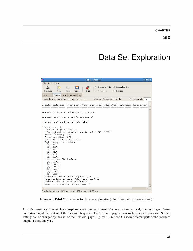
Figure 6.1: Febrl GUI window for data set exploration (after ‘Execute’ has been clicked).

It is often very useful to be able to explore or analyse the content of a new data set at hand, in order to get a betterunderstanding of the content of the data and its quality. The ‘Explore’ page allows such data set exploration. Severalsettings can be changed by the user on the ‘Explore’ page. Figures 6.1, 6.2 and 6.3 show different parts of the producedoutput of a file analysis.

21

Select data set to explore: This check boxes (only one is sensitive for a standardisation or deduplication project)determine which data set will be analysed. For a linkage, if a user only wants to analyse one of the two data sets theother data set can be un-checked.

Analyse values or words: With this two radio buttons the user can choose to either analyse the complete values in thedata set fields (attributes, columns), or split these values into words and analyse the word frequencies rather than thevalue frequencies.

For example, assume a user wants to analyse a data set containing an (un-standardised) field ‘name’ with the followingfour records:

namepeter christenpeter millerjoe meyerpeter meyer

An analysis of values (left) and words (right) , respectively, would return the following frequency counts:

Field 0: "name" Field 0: "name"Number of unique values: 4 Number of unique values: 4Most frequent values: Most frequent values:(1, ’peter christen’) (3, ’peter’)(1, ’peter miller’) (2, ’meyer’)(1, ’joe meyer’) (1, ’christen’)(1, ’peter meyer’) (1, ’joe’)

(1, ’miller’)

Use sample: If this box is checked and a number between 1 and 100 is entered (assumed to be a percentage value),then only a random sample of all the records will be analysed (i.e. all not selected records will simply be skipped over).This allows faster data set exploration for very large data set at the costs of less accurate analysis results.

As default, sampling is activated and 10% of all records will be randomly selected and analysed.

6.1 Data exploration results reported

Data set exploration is started with a click on ‘Execute’, and all results of the analysis will be reported into the mainFebrl GUI page area. For each field (column, attribute) in an explored data set the following basic statistics arecollected and reported for the sampled records (as shown in Figure 6.1):

• The number of unique values.

• The smallest and largest values (as strings).

• The average frequency and standard deviation of the values.

• A list of quantiles of the values.

• The six most and least frequent values and their counts (number of sampled and analysed records containingthat value).

• The minimum and maximum length in characters of the analysed values.

22 Chapter 6. Data Set Exploration

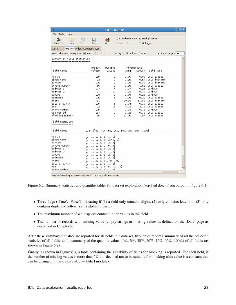
Figure 6.2: Summary statistics and quantiles tables for data set exploration (scrolled down from output in Figure 6.1).

• Three flags (‘True’, ‘False’) indicating if (1) a field only contains digits, (2) only contains letters, or (3) onlycontains digits and letters (i.e. is alpha-numeric).

• The maximum number of whitespaces counted in the values in this field.

• The number of records with missing value (empty strings or missing values as defined on the ‘Data’ page asdescribed in Chapter 5).

After these summary statistics are reported for all fields in a data set, two tables report a summary of all the collectedstatistics of all fields, and a summary of the quantile values (0%, 5%, 25%, 50%, 75%, 95%, 100%) of all fields (asshown in Figure 6.2).

Finally, as shown in Figure 6.3, a table containing the suitability of fields for blocking is reported. For each field, ifthe number of missing values is more than 5% it is deemed not to be suitable for blocking (this value is a constant thatcan be changed in the dataset.py Febrl module).

6.1. Data exploration results reported 23

Figure 6.3: Table with suitability for blocking of data set fields (scrolled down further from output in Figure 6.2).

For fields suitable for blocking, the number of resulting record pairs is calculated for a deduplication, i.e. for a valuewith count c the number of record pair comparisons that would result from this value is calculated as n = c(c − 1),and the total number of record pair comparisons is the sum of all n’s over all field values.

24 Chapter 6. Data Set Exploration

CHAPTER

SEVEN

Data Set Standardisation

Figure 7.1: Date component standardiser.

If ‘Standardisation’ has been selected as Febrl project type, then after a data set has been initialised on the ‘Data’page and ‘Execute’ was clicked to confirm this, then a page ‘Standardise’ will appear between the ‘Explore’ and ‘Log’pages.

Data cleaning and standardisation is based on four different types of component standardisers (for dates, telephonenumbers, names and addresses). It is possible to initialise more than one component standardiser of the same typeoperating on different fields of a data set. For example, if a hospital data set contains a date-of-birth and a date-of-admission field one data standardiser each would be required.

When a standardisation project is started (on the ‘Output/Run’ page as described in Chapter 11), the initialised dataset is loaded, cleaned and standardised, and written into a standardised output data set (with a file name to be definedon the ‘Output/Run’ page).

A new component standardiser can be added with a click on the corresponding button. If one or more componentstandardisers have been generated, it is also possible to delete the last one (i.e. the one just above the row of buttonsbelow the last component standardiser, as for example shown in Figure 7.1). At least one component standardiser hasto be initialised before ‘Execute’ can be clicked, as otherwise no standardisation would be conducted.

Input fields: All component standardisers on the left side have a pull-down menu that lists the names of all fieldsfrom the input data set. The user can select one of these fields to be used for a component standardiser (for example,

25

in Figure 7.1 the ‘date of birth’ field will be standardised using a date standardiser).

It is possible to have more than one input field for a component standardiser, by clicking on the ‘Add a new inputfield’ button, which will result in a new pull-down menu appearing. If more than one input field is selected, then thevalues from these fields will be concatenated with the ‘Field separator’ value given in the ‘Parameters’ section of thecomponent standardiser (see description below). For example, the name component standardiser in Figure 7.3 has thetwo input fields ‘given name’ and ‘surname’, which will be concatenated (with a – not visible – whitespace charactergiven in the field separator parameter).

Output fields: On the right side of each component standardiser is a list of output fields, which ranges from three (fora date standardiser) to 27 (for an address standardiser) fields. The values in the text entry areas give default values forthe field names to be used in the standardised output data set. These field names can be changed by a user. If such atext entry is set to an empty string or to ‘None’ (as shown in Figure 7.3), then the corresponding output field will notbe written into the standardised output data set. For example, no title or gender guess fields will be written into theoutput data set for the name standardiser initialised in Figure 7.3.

Parameters: Several parameters that have to be set by the user are shown in the middle column of a componentstandardiser, between the input fields on the left and the output fields on the right. Some of these parameters arecommon to all component standardiser types and are described below, while parameters specific to a componentstandardiser type will be described in the corresponding following sections.

• ‘Field separator’This parameter is a string which will be used to concatenate the field values from the input fields, if more thanone input field is initialised for a component standardiser. The default value is an empty string.

• ‘Check word spill’If this check box is activated and the field separator is set to a non-empty string (for example a whitespacecharacter), and more than one input field is initialised, then word spilling from one input field into another willbe checked using the words listed in the tag tables initialised for the component standardiser.

Word spilling can happen when data is entered into fields with fixed length, and continuous typing by theperson doing the data entry automatically continues into the next field once a field is full. For example, if agiven name field with maximal length of 10 characters is given, and a surname field with 20 characters, thenthe name ‘maria louisa miller’ would be stored as given name ‘maria loui’ and surname ‘samiller’. To check for word spilling can be a successful data cleaning step if a data set contains such spilledword data.

Word spilling concatenates words at the end of one input field and the beginning of the next input field and thenchecks if such a concatenated word is known, i.e. if it is listed in one of the initialised tag lookup tables. Ifso, the concatenated word is kept, otherwise (i.e. if the word is not known) the field separator will be insertedbetween the two original words.

Execute A click on the ‘Execute’ button will result in the validation of all input and output fields, and parametersettings of the initialised component standardisers. An error window will appear if any of the given settings is notvalid, detailing what is wrong.

If all required settings are complete and valid, the Febrl Python code corresponding to data standardisation will begenerated and stored internally, and shown on the ‘Log’ page (see Chapter 13 for more detail on the ‘Log’ page).

After a successful ‘Execute’ the ‘Output/Run’ page will appear (described in detail in Chapter 11), which will allowthe running of a Febrl standardisation project.

26 Chapter 7. Data Set Standardisation

7.1 Date standardisation

A date component standardiser will standardise the values from the input field (or fields) into three output fields: day,month, and year (as shown in Figure 7.1). These output fields can be set to an empty string or ‘None’ if no output isto be written into the corresponding output field, as long as at least one output field is not empty or ‘None’.

A date component standardiser has the following two parameters:

• ‘Parse formats’This has to be a list containing one or several strings (separated by commas) with a date parsing format. Eachparsing format must contain three of the following format strings with a space between them (such as ‘%d %m%Y’):

– %d Day of the month as a decimal number (between 1 and 31).

– %b Abbreviated month name (Jan, Feb, Mar, etc.).

– %B Full month name (January, February, etc.).

– %m Month as a decimal number (between 1 and 12).

– %y Year without century as a decimal number (between 0 and 99).

– %Y Year with century as a four-digit decimal number.

Besides the spaces between the three parsing directives, format strings must not contain any other characters,such as ‘:’, ‘-’, etc. as they will be removed from the input values before date parsing is attempted.

For example, the parse format ‘%d %m %Y’ will correctly parse strings such as ‘13 05 2007’,‘31-12-1999’, ‘1/01/1919’, etc.

During standardisation of a date string from the input field(s), the parsing routine tries one format after the otherand the first format that successfully parses the input string into a valid date will be used. Therefore, date formatsthat are more commonly appear in the input data set should be at the top of the parse format list.

• ‘Pivot year’This has to be a value between ‘00’ and ‘99’ which controls the expansion of two-digit year values into four-digit year values. A two-digits year ‘XX’ smaller than the pivot year will be expanded into ‘20XX’, while yearsequal to and larger than the pivot year will be expanded into ‘19XX’. For example, with a pivot ear set to ‘03’, atwo-year value of ‘68’ will be expanded into ‘1968’, a value ‘03’ into ’1903’, and a value ’02’ into ‘2002’. Thedefault pivot year value given in the Febrl GUI is the current year plus 1.

7.2 Telephone number standardisation

The telephone number component standardiser is based on rules and standardises the values from the input field(s)into five output fields as shown in Figure 7.2: country code (i.e. international dialling code), country name, area code,number, and a possible extension.

Beside the field separator parameter, one more additional parameter has to be set for this component standardiser.

• ‘Default country’This parameter can be set to either ‘Australia’ or ‘Canada/USA’, with the former being the default value. Itinfluences the rule based standardisation approach on how telephone numbers are parsed in a country specificway.

7.1. Date standardisation 27

Figure 7.2: Telephone number component standardiser.

7.3 Name standardisation

The name component standardiser is based on rules for simple names (made of one or two words after a possible titleword has been removed) or hidden Markov models (HMMs, as described in Section 7.6 below) for more complexnames consisting of more than two words.

A name value from the input field(s) is standardised into the six output fields title, gender guess, given name, alternativegiven name, surname, alternative surname (as shown in Figure 7.3).

Beside the field separator and check word spilling parameters, this component standardiser requires both HMM relatedparameters (described in Section 7.6 below) as well as the definition of a correction list and one or more tag lookuptables (which will be discussed in Section 7.5 below).

The three name component standardiser specific parameters are:

• ‘Female titles’This can be a list of one or more (comma separated) words that are assumed to be female title words, such as‘ms’, ‘miss’, or ‘mrs’. They will be used for the guessing of the gender of an input name value.

• ‘Male titles’This is similar to female title, but should contain male title words, such as ‘mr’ or ‘mister’.

• ‘First name component’This can either be set to ‘Given name’ (the default) or ‘Surname’, and will provide a hint to the name standardi-sation routine on which name component will likely appear first in the name values loaded from the input dataset.

7.4 Address standardisation

The address component standardiser is fully based on hidden Markov models (HMMs) (see Section 7.6 below), andstandardises addresses into the following 27 output fields: building name, post address type, post address number, lotnumber prefix, lot number, lot number suffix, flat number prefix, flat number, flat number suffix, flat type, level number


Figure 7.3: Name component standardiser.

prefix, level number, level number suffix, level type, number first prefix, number first, number first suffix, number lastprefix, number last, number last suffix, street name, street suffix, street type, locality name, postcode, state abbrev,and country. These output fields correspond to the fields used in the Australian G-NAF (Geocoded National AddressFile)1.

Besides the common parameters (field separator and word spill checking), HMM related parameters, and correctionlist and lookup tables, no address specific parameter is required.

7.5 Correction lists and tag lookup tables

Correction list contain strings (characters or words) and their replacements. They are used in the initial cleaning stepin the data standardisation process. Tagging lookup table, on the other hand, also contain strings and their replacement,but additionally groups of table entries are assigned a tag, which is used in the tagging step within the name or addressstandardisation process.

Note: Example correction lists and tag lookup tables are supplied with the Febrl distribution. They do contain valuesbased on Australian addresses, as well as names collected from Australian sources. Therefore, these files have tobe changed and adjusted to different domains, especially different countries which likely have both different addressvalues and possibly different (language specific) name values.

Both correction lists and tag lookup tables can be initialised to corresponding text files for name and address componentstandardisers on the Febrl GUI. Their file formats is described in the following two sections.

7.5.1 Correction lists

Correction list files contain characters or strings and their corresponding corrections (replacements). They are con-verted into lists that are used in the initial data cleaning step to replace a character or string with the correspondingreplacement.

Correction list files should have a file extension ‘.lst’. The format of these files is as follows:1 http://www.g-naf.com.au

7.5. Correction lists and tag lookup tables 29

http://www.g-naf.com.au

• An entry in the correction-list file is of the form

replacement := values

where values is a list of one or more strings separated by commas. Each value in this list is replaced with thereplacement character or string on the left hand-side of the entry.

• All replacement and value strings have to be quoted, either with single or double quotes.

• An entry can be longer than one line, in which case the second and following lines consist of the values list only.

• Comment lines are lines that start with a ‘#’ character.

The following example is taken from the ‘name corr.lst’ file as available in the data/lookup folder of the Febrldistribution):

# ====================================================================

# Remove characters and words from input’ ’ := ’.’, ’?’, ’˜’, ’_’, ’:’, ’;’, ’ˆ’, ’=’, ’ n a ’,

’*’, ’ n/a ’, ’ n.a. ’, ’\’, ’ also ’, ’ name ’,’ only ’, ’ abbrev ’, ’ initials ’, ’ unk ’,’ unkn ’, ’ missing ’, ’ unknown ’

# Correct words and symbols’ and ’ := ’+’, ’&’’ baby ’ := ’ babe ’

’ baby of ’ := ’ babyof ’, ’ babeof ’, ’ b/o ’, ’ b.o.’’ daughter of ’ := ’ daughterof ’, ’ d/o ’, ’ d.o.’

’ son of ’ := ’ sonof ’, ’ s/o ’, ’ s.o.’’ known as ’ := ’ knownas ’, ’ a.k.a. ’, ’ aka ’

’ - ’ := ’-’, ’/’’ ( ’ := ’<’, ’(’, ’[’, ’’’ ) ’ := ’>’, ’)’, ’]’, ’’’ | ’ := ’"’, "’", ’|’

# Remove ’ from o’brian etc’ o’ := " o’"’ a’ := " a’"’ l’ := " l’"’ i’ := " i’"’-o’ := "-o’"

In the above example, all values in the first entry (an entry that goes over four lines) are replaced with a single space’ ’. It is important that, for example, the value ’ na ’ starts with a space and ends with a space. Assuming thesespaces were omitted, i.e. the value would be ’na’, then each occurrence of the string ’na’ in the input would bereplaced by a single space. The word ’annabella’ would thus be replaced with ’an bella’ which is not whatis wanted.

The list of value and replacement pairs is internally sorted with decreasing length of the values. Long value strings aretherefore replaced before shorter strings or characters are replaced. In this way, the value ’ a.k.a. ’ is replacedwith ’ known as ’ before full-stops (periods) ’.’ are replaced by a space ’ ’.

7.5.2 Tag lookup tables

A tag lookup table file contains one or more blocks of entries, with all entries in a block being assigned the same tag.Tag lookup table files should have a file extension ‘.tbl’. The format of these files is as follows:


• A block starts with a line that contains a tag assignment with a tag in brackets:

tag=<tag>

This tag assignment must be written at the beginning of a line. It is possible to have a comment (starting with a‘#’) after the assignment.

• All following lines are assumed to contain the entries to be tagged with the currently assigned tag, until a linewith a new, different tag assignment is encountered.

• Each entry in a block is of the form:

key : values

where values is a list of none, one or more strings (not quoted) separated by commas, and key (not quoted) isone or several words.

• Each of the values in the list will be replaced with the key if found in an unstandardised input field.

• If the values list is empty, then only the key itself will be inserted into the lookup table.

• A key and a value can consist of more than one word, separated by spaces.

• If a value occurs in more than one block and it is replaced with the same key but with different tags, all tags arekept and stored in a list for this value.

• If a value occurs in more than one block and it is replaced with different keys, an error message is triggered andthe program stops. The user then manually has to correct this conflict in the tag lookup file(s).

• Comment lines are lines that start with a ‘#’ character.

The following examples are extracted from the ‘name misc.tbl’ file as available in the data/lookup folder of theFebrl distribution):

# ====================================================================

tag=<SP> # Tag for separator elementsand :or :

known as : kn as, kn, known

tag=<BO> # Tag for ’baby of’ and similar sequencesbaby :

baby of :daughter :

daughter of :son :

son of :

tag=<NE> # Tag for word ’nee’ (born as) or surname or givenname (?)nee :

7.5. Correction lists and tag lookup tables 31

7.6 Hidden Markov models

Hidden Markov models (HMMs) have to be initialised for both the name and address component standardisers. Twoexample HMM files are available in the hmm folder of the Febrl distribution.

Training for name and address hidden Markov models (HMMs) currently has to be done outside of the Febrl GUIusing the trainhmm.py program, which contains instructions about the format of HMM training data.

For a more comprehensive discussion on the HMM approach to name and address standardisation please refer to thefollowing paper [11] (which is available in the docu folder of the Febrl distribution):

Preparation of Name and Address Data for Record Linkage using Hidden Markov Models.Tim Churches and Peter Christen and Kim Lim and Justin X. Zhu.BioMed Central Medical Informatics and Decision Making, vol. 2, no. 9, 2002. doi:10.1186/1472-6947-2-9


CHAPTER

EIGHT

Indexing (Blocking) Page

Figure 8.1: Example ‘Index’ page showing an initialised sorting index with three indices, the first made of two indexdefinitions and the second and third made of one index definition.

The ‘Index’ page allows the user to select one of the several indexing (blocking) techniques implemented in Febrl, aswell as to select the input fields and their possible encodings to be used in the index definitions.

The parameter settings required for the different indexing techniques currently implemented in Febrl are describedbelow, with the definition of the actual indices being described in Section 8.10. For more technical details please referto the technical report [7] (which is available in the docu folder of the Febrl distribution):

Towards Parameter-free Blocking for Scalable Record Linkage.Peter Christen.ANU Computer Science Technical Report Series, TR-CS-07-03, August 2007.Department of Computer Science, Faculty of Engineering and Information Technology,The Australian National University, Canberra.

33

All indexing techniques (except the ‘FullIndex’ described in Section 8.1) require the setting of two parameter.

• ‘Separator string’If an index is made of more than one index definition (as shown for example with ‘Index 1’ in Figure 8.1), thenthe field values used in this index will be concatenated with this separator string in-between. The default valueis an empty string.

• ‘Skip missing’If this check box is activated (the default), then empty indexing values (i.e. field values that are empty strings)will not be inserted into the index. If de-activated, this will result in a block being generated containing allrecords that have empty index definition values.

Execute: With a click on the ‘Execute’ button the chosen indexing technique and index definition(s) and all theirparameter settings are validated, and if any is not valid a corresponding error window will appear detailing what hasto be changed.

Once all settings are valid, the Febrl Python code for the selected index technique and its index definition(s) will begenerated, stored internally and shown on the ‘Log’ page.

8.1 Full index

This technique will perform no indexing but conduct the full comparison of all record pairs (quadratic complexity inthe size of the number of records in the two data sets).

No parameters have to be set for this indexing technique, and neither do index definitions have to be defined.

8.2 Blocking index

This technique implements the ‘standard’ blocking index traditionally being used for record linkage. Records that havethe same values in an index definition are put into the same block, and only records within a block are then comparedwith each other.

No parameters have to be specified for this blocking technique. It is however possible to select that the actual im-plementation to be used is either the ‘BigMatch’ indexing for a linkage or the ‘DedupIndex’ for a deduplication, asdiscussed in Sections 8.8 and 8.9 below.

8.3 Sorting index

This technique is based on the sorted window approach, where a window that includes a certain number of indexvalues is moved over the sorted values of the index definitions.

The parameter that needs to be selected is the ‘Window size’ which has to be a positive integer number. If set to 1,then sorting index becomes the same as the standard blocking index (i.e. only records that have exactly the same indexdefinition values will be compared).

Similar to blocking index, it is possible to use the ‘Bigmatch’ or ‘Dedup’ index implementation.

34 Chapter 8. Indexing (Blocking) Page

8.4 Q-gram index

This indexing technique allows for fuzzy blocking with overlapping blocks, similar to canopy clustering describedbelow. The basic idea is to convert the index values into lists of q-grams, and to build sub-lists of these using athreshold (a number between 0.0 and 1.0) containing all possible combinations. Records will be inserted into morethan one block.

For example, assume q = 2 (bigrams), the threshold set to 0.8, and a record that has an indexing value ‘peter’. Thisvalue will first be converted into the q-gram list [‘pe′, ‘et′, ‘te′, ‘er′] with four elements. With a threshold of 0.8,4 ∗ 0.8 = 3.2, then rounded to 3. Thus, all sub-list combinations of length 3 are calculated for this q-gram list. Theyare:

[‘pe′, ‘et′, ‘te′][‘pe′, ‘et′, ‘er′][‘pe′, ‘te′, ‘er′][‘et′, ‘te′, ‘er′]

Converted back into strings, all records that have an index value ‘peter’ will be inserted into the index blocks with keys‘peette’, ‘peeter’, ‘peteer’ and ‘etteer’.

For this indexing technique, the following parameters have to be set:

• ‘Length of Q’This has to be a positive integer value which determines the lengths of the q-grams to be used. Commonly usedvalues are 2 (bigrams) and 3 (trigrams).

• ‘Threshold’This has to be a number larger than 0.0 and smaller than 1.0. If set to 1.0 q-gram blocking would become thesame as the standard blocking index, i.e. only records that have exactly the same index definition values will becompared.

• ‘Padded’If this check box is activated, then the beginning and end of the input strings will be padded with (q − 1)special characters, in order to get specific q-grams that indicate the beginning and end of a string. For example,if padded is activated, the list of bigrams for the input string ‘peter’ will be (assuming ‘#’ is the special startcharacter and ‘@’ the end character): ‘#p, ‘pe’, ‘et’, ‘te’, ‘er’, and ‘r@’, while without padding the bigram listwould be ‘pe’, ‘et’, ‘te’, and ‘er’.

Similar to blocking index, it is possible to use the ‘Bigmatch’ or ‘Dedup’ index implementation, as discussed inSections 8.8 and 8.9 below.

8.5 Canopy clustering index

This index technique uses canopy clustering to generate overlapping blocks (clusters). These clusters will be formedusing q-grams and are based on using as similarity measure either TF-IDF (Term-Frequency Inverse Document Fre-quency, as commonly used in information retrieval) or simply calculating the proportion of common q-grams (anapproximation to the Jaccard similarity). Similar to q-gram based indexing, each record will be inserted into severalblocks. For more technical details about this indexing technique please see [3, 7].

The following parameters have to be set for this indexing technique:

• ‘Canopy method’This can be set to ‘TF-IDF’ or ‘Jaccard’. It is the similarity measure based on the q-grams formed from theindex values. This will determine the way the canopy clusters are being formed. Please see [7] for more details.

8.4. Q-gram index 35

• ‘Threshold’This determines the way the size of the overlapping clusters is being calculated. It can be set to either ‘Global’or ‘Nearest’. For both, two different parameter values have to be entered into the following ‘Parameters’ textentry.

• ‘Parameters’For the global threshold method, two threshold values between 0.0 and 1.0 have to be given (separated by acomma, for example ‘0.8, 0.6‘), with the first value being the tight threshold and the second value the loosethreshold. The tight threshold has to be larger than or equal to the loose threshold value.For the nearest method, two integer values (giving the number of tight and loose nearest records) have to begiven. In this case, the tight nearest number has to be smaller or equal to the loose number of nearest.

• ‘Length of Q’Same parameter as described in Section 8.4 above.

• ‘Delete percentage’This can be set to a percentage threshold value between 1 and 100 (the default), which will set a threshold forremoving common q-grams from the index (i.e. if they appear in more than this percentage of all records). Asdefault no q-grams will be removed.

• ‘Padded’Same parameter as described in Section 8.4 above.

8.6 String map index

The basic idea is of this indexing technique is to map the strings in the index definition into a multi-dimensional spacethat preserves the (Euclidean) distances over strings, and to use an efficient multi-dimensional data structure to retrievesimilar pairs of strings. For more details on the technical details of this indexing technique please refer to [19]. Theimplementation of this technique in Febrl is modified from the originally proposed approach and is combined withthe canopy clustering technique described above in Section 8.5. For more details please see [7].

The following parameters have to be set for this indexing technique:

• ‘Canopy method’Similar to the canopy method described above in Section 8.5, this parameter determines how the nearest (mostsimilar) strings are extracted into clusters. Possible methods are ‘TF-IDF’ or ‘Jaccard’.

• ‘Parameters’The parameters used for the canopy method, the same as described above in Section 8.5.

• ‘Grid resolution’The multi-dimensional data structure is based on a grid, and this parameter gives the number grid cells in eachdimension. It has to be set to a power of 10 integer number (e.g. 10, 100, 1000, etc.).

• ‘Dimension’The dimension of the space into which strings are mapped. This has to be a positive integer number, normallyin the range of around 10 to 20.

• ‘Sub-dimension’This will be the dimension used by the indexing technique to extract records from the multi-dimensional space.It has to be a positive number smaller or equal to the main dimension chosen.

• ‘Similarity function’The string distance function to be used when finding distances between pairs of strings when mapping theminto a multi-dimensional space. Distances are calculated as (1.0− sim) with a normalised similarity value simbetween 1.0 (strings are the same) and 0.0 (strings are totally different).


• ‘Cache distance calculations’If this check box is activated, then the results of all distance calculations between pairs of strings (in a multi-dimensional space) are cached for increased performance (as the same pair of strings is likely to be comparedseveral times). If this caching is activated more memory will be required.

8.7 Suffix array index

This index technique is based on the idea of creating a sorted suffix array of the index values, and extracting blocksfrom this array with constraints of a maximum block size. Technical details can be found in [1, 7].

The suffixes of a string are all the sub-strings of the string with the beginning removed down to a minimum length.For example, for the string ‘christen’ and minimum length set to 2, the corresponding suffix strings will be ‘hristen’,‘risten’, ‘isten’, ‘sten’, ‘ten’, and ‘en’.

The following four parameters have to be set for this indexing technique:

• ‘Minimum length’The minimum length of sub-strings to be generated and stored in the suffix-array. These sub-strings will be usedas index (block) key values. This has to be a positive integer value.

• ‘Maximum block size’The maximum records in a block which will be used in the index process (i.e. the maximum number of recordswith the same index value). Blocks that contain more records will be ignored. For example, with the string‘christen’ given above, many more records will be entered into the block for the suffix string (index value) ‘en’than for the index value ‘sten’, and the block ‘en’ will likely be too big (generating too many record pairs) andtoo unspecific.

• ‘Suffix method’This parameter determines how suffix strings are generated. If set to ‘All sub-strings’, then all possible sub-strings will be generated (not just the suffix strings). For example, for a string ‘peter’ the following sub-stringswill be generated: ‘pete’, ‘eter’, ‘pet’, ‘ete’, ‘ter’, etc.

If set to ‘Suffix only’ then only the true suffixes are generated. For example for ‘peter’, the sub-strings ‘eter’,‘ter’, ’er’, etc. will be generated.

• ‘Padded’Same parameter as described in Section 8.4 above. If activated, the strings will be padded before their suffixstrings will be generated.

8.8 ‘BigMatch’ index

The ‘BigMatch’ index implements ideas from the Bigmatch record linkage project developed by the US Census Bu-reau. Please refer to [21] for more details.

This index can only be used when linking two data sets, but not when deduplicating one data set. The basic idea is toload and process the smaller of the two data sets to be linked, such that an index of this smaller data set that allowsefficient access to all records in a block is stored in main memory. Then, the larger data set is loaded, and each of itsrecords has only to be accessed and processed once (it will be compared to all records from the smaller data set in thesame block).

The ‘BigMatch’ indexing technique can only be used with the blocking index (Section 8.2), sorting index (Section 8.3),and q-gram index (Section 8.4), because the other indexing techniques require both data sets to be completely loadedand processed before record pairs can be compared.

8.7. Suffix array index 37

8.9 Deduplication index

This index technique is specialised for the deduplication of one data set. It works by loading the data set to bededuplicated, and when a record is read it is immediately processed (i.e. its index values are extracted and generated)and it is inserted into a indexing data structure in main memory that keeps all records in the same block together. Eachrecord is then compared to all previously read and processed records that are stored in the same block in main memory.

Similar to the ‘BigMatch’ index, this index technique can only be used with the blocking index (Section 8.2), sortingindex (Section 8.3), and q-gram index (Section 8.4), because the other indexing techniques require that a data set iscompletely loaded and processed before record pairs can be compared.

8.10 Index definitions

Once an index technique has been selected and all its parameters have been set, the actual index (or blocking) defini-tions have to be set up. In Febrl, one or more indices can be defined as described below, each made of one or moreindex (or block) definitions.

The example shown in Figure 8.1 shows three indices, the first made of two index definitions, and the second andthird made of one index definition each. For this example, the first index (block) values will be formed by takingthe values from the ‘surname’ field in the input data set, encoding them using the ‘Double-Metaphone’ method [6](and only taking the first three characters of these codes), and then concatenating these three-character codes with thevalues from the ‘postcode’ field taken from the same input record. All records that have the same index value willthen be inserted into the same block. For the second index, all records that have the same ‘Soundex’ encodings [6]of their ‘suburb’ values will be inserted into the same block. Finally, for the third index the values from the inputfield ‘suburb’ are first sorted (if they include several words), and then reversed before again being encoded using the‘Sounds’ technique. Again, all records that have the same encoded value will be inserted into the same block. For thefollowing three example records, the input as well as the corresponding three index (block) values are shown:

rec_id, surname, postcode, suburb__rec_id__-0, miller, 2010, west sydney__rec_id__-1, christen, 0200, canberra__rec_id__-2, smith, 3123, south west rocks

Index values from the first index definition:

__rec_id__-0: mlr2010__rec_id__-1: krs0200__rec_id__-2: sm03123

Index values from the second index definition:

__rec_id__-0: w232__rec_id__-1: c516__rec_id__-2: s323

Index values from the third index definition:

__rec_id__-0: a615__rec_id__-1: t253__rec_id__-2: t232


8.10.1 Index definition parameter settings

For each index definition, the following parameters can be set.

• ‘Field name’ (for deduplication)‘Field name A’ and ‘Field name B’ (for linkage)These designate the field name(s) from the input data set(s) to be used for an index definition. For a linkage,these should be fields that contain the same piece of information (for example two fields that both containsurnames, or both contain postcodes).

• ‘Maximum length’The maximum length of the index variable generated for this index definition. Longer values will be truncated.

• ‘Sort words’If this check box is activated, an input value that contains more than one word (i.e. contains a least one whites-pace character) will first be sorted word-wise (the suburb names from the above would be sorted into ‘sydneywest’ and ‘rocks south west’, respectively).

• ‘Reverse’If this check box is activated then the input values will be reversed (after the possibly have been sorted, butbefore they are phonetically encoded). For example, a value ‘canberra’ will be reversed into ‘arrebnac’.

• ‘Encoding function’With this drop-down menu the user can select the (phonetic) encoding method to be used on the index valuestrings. Currently available encoding methods are: ‘Soundex’, ‘Modified Soundex’, ‘Fuzzy Soundex’, ‘Double-Metaphone’, ’NYSIIS’, ‘Phonex’ and ‘Phonix’. For more details on these functions please see [6], as well astheir implementations in the Febrl module encode.py.

It is also possible to not encode the index value strings by selecting ‘None’, or to extract a sub-string from theindex values by selecting the ‘Sub-string’ method. In that case, the start and end (two integer numbers separatedby a comma) of the sub-string to be extracted have to be given in the ‘Encoding function parameters’ text entryfield. These numbers assume that the first character in a string has index 0. For example, with start and end setto ‘2,6’ and an input value string ‘canberra’, then the index (block) value to be used would be ‘nber’.

• ‘Encoding function parameters’This text entry field is currently only used for the ‘Sub-string’ encoding method as described above.

8.10. Index definitions 39

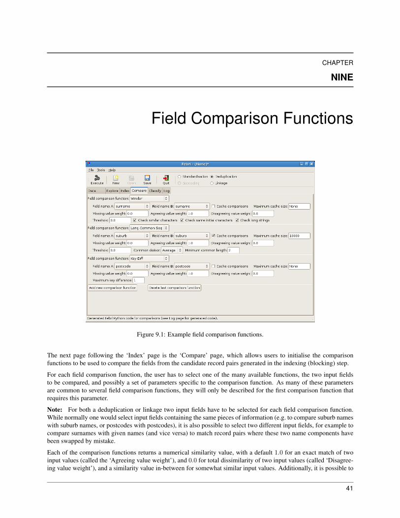
CHAPTER

NINE

Field Comparison Functions

Figure 9.1: Example field comparison functions.

The next page following the ‘Index’ page is the ‘Compare’ page, which allows users to initialise the comparisonfunctions to be used to compare the fields from the candidate record pairs generated in the indexing (blocking) step.

For each field comparison function, the user has to select one of the many available functions, the two input fieldsto be compared, and possibly a set of parameters specific to the comparison function. As many of these parametersare common to several field comparison functions, they will only be described for the first comparison function thatrequires this parameter.

Note: For both a deduplication or linkage two input fields have to be selected for each field comparison function.While normally one would select input fields containing the same pieces of information (e.g. to compare suburb nameswith suburb names, or postcodes with postcodes), it is also possible to select two different input fields, for example tocompare surnames with given names (and vice versa) to match record pairs where these two name components havebeen swapped by mistake.

Each of the comparison functions returns a numerical similarity value, with a default 1.0 for an exact match of twoinput values (called the ‘Agreeing value weight’), and 0.0 for total dissimilarity of two input values (called ‘Disagree-ing value weight’), and a similarity value in-between for somewhat similar input values. Additionally, it is possible to

41

set a special numerical value for the case where one (or both) of the input values is missing (i.e. is an empty string),called the ‘Missing value weight’. All three values can be modified by the user on the GUI. It is important that foreach comparison function:

1. The disagreeing weight value has to be lower than the agreement weight value.

2. The missing weight value has to be between the disagreement and the agreement weight values.

In the following sections all available field comparison functions will be described. For a more detailed discussionon name matching and an evaluation of many of these comparison function please refer to the following technicalreport [6] (which is available in the docu folder of the Febrl distribution):

A Comparison of Personal Name Matching: Techniques and Practical Issues.Peter Christen.ANU Computer Science Technical Report Series, TR-CS-06-02, September 2006.Department of Computer Science, Faculty of Engineering and Information Technology,The Australian National University, Canberra.

Execute: With a click on the ‘Execute’ button the chosen field comparison functions and their settings are validated,and if any setting is not valid a corresponding error window will appear detailing what has to be corrected.

Once all settings are valid, the Febrl Python code for the defined field comparison functions will be generated, storedinternally and shown on the ‘Log’ page (see Chapter 13 for more details).

Note: The user is encouraged to fully define one field comparison function after the other, and click ‘Execute’after each in order to confirm its settings. Due to the GUI characteristics, earlier chosen settings that have not beenconfirmed via a click on ‘Execute’ might be lost when a new field comparison function is added.

9.1 Exact string comparison

In this simple comparison function input values (assumed to be strings) are compared exactly, and if they are the samethe agreeing value weight will be returned (default value 1.0), otherwise the disagreeing value weight (default 0.0).If one or both of the input values is missing (is an empty string) then the missing value weight (default 0.0) will bereturned.

9.2 Contains string comparison

This field comparison function checks if the shorter of the two input string values is fully contained in the longer ofthe two input strings, and if so returns the agreement value weight, otherwise it returns the disagreement value weight.If one or both of the input values is missing then the missing value weight will be returned.

9.3 Truncated string comparison

This comparison function allows setting of a maximum string length (using the parameter ‘Number of characters tocompare’), so that only the beginning of the two strings will be compared using exact string comparison as describedin Section 9.2 above.

42 Chapter 9. Field Comparison Functions

9.4 Key difference comparison

This field comparison function compares the values in the two input fields character-wise and counts all characterdifferences, with a maximum number of different characters being tolerated. This comparison function can be used tocompare both textual and numerical fields, such as postcodes or telephone numbers. For example, the two postcodes‘1234’ and ‘1284’ have a key difference of 1 (‘3’ and ‘8’), while the pair of telephone numbers ‘6125 5680’and ‘8152-6581’ has a key difference of 7 (‘6’ and ‘8’, ‘2’ and ‘5’, ‘5’ and ‘2’, ‘ ’ and ‘-’, etc.).

The parameter ‘Maximum key difference’ sets the maximum number of different keys (characters) that is tolerated. Ifmore than the maximum number of key differences is counted, then the disagreement value weight will be returned,while if the number of key differences is below that maximum number the following formula will be used to calculatea partial agreement value weight:

partial agree weight = agree weight− num key diff

max num key diff + 1∗ (agree weight + abs(disagree weight)),

with num key diff the counted number of key differences in a pair of input values, and max num key diff themaximum tolerated number as specified in the Febrl GUI.

9.5 Numeric percentage comparison

This is a field comparison function for numeric field values, where a given percentage difference will be tolerated. Theagreement value weight is returned if the numbers are the same, and the disagreement value weight if the percentagedifference between the two numbers is larger than a maximum tolerated percentage value. The disagreement valueweight will also be returned if either of the two input values is not a number.

The ‘Maximum percentage difference’ parameter has to be set to a percentage value between 0 and 100. If set to 0,this field comparison function reduces to exact numerical comparison.

The percentage difference between two input values, value1 and value2 (both assumed to be numbers), is calculatedas:

perc diff = 100.0 ∗ abs(value1 − value2)max(abs(value1), abs(value2))

.

If the calculated perc diff percentage difference is smaller than the maximum percentage max perc diff (as set onthe GUI) tolerated, then a partial agreement weight is calculated according to the following formula:

partial agree weight = agree weight− perc diff

max perc diff + 1.0∗ (agree weight + abs(disagree weight)).

9.6 Numeric absolute comparison

This field comparison function is for numeric field values, where a given absolute numerical difference will be tol-erated. The agreement value weight is returned if the numbers are the same, and the disagreement value weight ifthe absolute difference between the two values is larger than the value given in the parameter ‘Maximum absolutedifference’ in the Febrl GUI. The disagreement value weight will also be returned if either of the two input values isnot a number.

If the absolute difference is equal or smaller than the max abs diff parameter value given on the GUI, then a partialagreement weight will be calculated according to the following formula:

partial agree weight = agree weight− abs(value1 − value2)max abs diff + 1.0

∗ (agree weight + abs(disagree weight)).

9.4. Key difference comparison 43

9.7 Encoded string comparison

This field comparison function is based on the idea of phonetically encoding the strings before they are compared. Ifthe phonetic codes of two input fields are the same, then the agreement value weight will be returned, if the codes aredifferent then the disagreement value weight will be returned, and if one or both strings are empty then the missingvalue weight will be returned.

The following three parameters have to be set for this comparison function.

• ‘Encoding function’One of the available phonetic encoding functions has to be selected. Currently available are: ‘Soundex’, ‘Mod-ified Soundex’, ‘Fuzzy Soundex’, ‘Double-Metaphone’, ’NYSIIS’, ‘Phonex’ and ‘Phonix’. For more details onthese functions please see [6], as well as their implementations in the Febrl module encode.py.

• ‘Reverse’If this check box is activated the input value strings will first be reversed before they are encoded. This canimprove comparison of values that have variations or errors at their beginnings (for example, ‘christina’ and‘kristina’ would be encoded into two different Soundex codes, while if they are reversed, ‘anitsirhc’ and ‘anit-sirk’ would have the same code).

• ‘Maximum code length’This value must be a positive integer and it limits the number of characters at the beginning of the two codesthat are being compared.

9.8 Distance based comparison

Not yet implemented into the Febrl GUI, please see the module comparison.py for more details on this fieldcomparison function.

9.9 Date comparison

This field comparison function compares two dates given as strings in one of several possible formats as given in theparameter ‘Date format’ as detailed below. This comparison function allows two tolerance ranges if the two inputdates differ by a certain number of days. Therefore, the agreement value weight will be returned if two input dates arethe same, the disagreement value weight will be returned if they are more than the provided maximum date differencesapart, and a partial agreement value weight will be returned if they are less than the maximum day range apart. Thedisagreement value weight will also be returned if either of the two input dates is not a valid tuple of numbers (e.g.month value larger than 12).


• ‘Maximum day A before day B’The maximum tolerated number of days that the first input date value can be before the second input date value.See below for a description of how this value will be used to calculate a partial agreement weight value.

• ‘Maximum day A after day B’The maximum tolerated number of days that the first input date value can be after the second input date value.See below for a description of how this value will be used to calculate a partial agreement weight value.

• ‘Date format’This has to be a format string that will be used to extract the date values from the input values. Possible are:‘ddmmyyyy’, ‘mmddyyyy’, ‘yyyymmdd’ ‘ddmmyy’, and ‘mmddyy’ (with ‘dd’ assumed to be the day number,‘mm’ the month number, ‘yy’ a two-digit year number, and ‘yyyy’ the year as a four digit number).


Note: Some cleaning will be done before the input date values are separated into day, month and year values.Specifically, commonly used separator characters, like ‘:’ or ‘-’, are removed from the input date values beforethey are compared.

If the first input day value is equal to or less than max day A before day B days before the second day value, thena partial agreement weight will be calculated as follows:

partial agree weight = agree weight− date diff

max day A before day B + 1∗(agree weight+abs(disagree weight)),

and similar, if the second day value is equal to or less than max day A after day B’ days after the first day valuethen a partial agreement weight will be calculated as follows:

partial agree weight = agree weight− date diff

max day A after day B + 1∗(agree weight+abs(disagree weight)),

with day diff the difference in days between the two input dates.

For two special cases, the partial agreement weight value is calculated as follows:

1. A swap partial agreement weight value will be calculated when the day and month values of the two input datesare swapped (and the year values are the same) according to the following formula:

partial agree weight = agree weight− 0.5 ∗ (agree weight + abs(disagree weight)).

For example, if the two day values are ‘[12,10,1999]’ and ‘[10,12,1999]’, then this swap agreement weight valuewill be calculated.

2. If the difference between the days is larger than max day A before day B or max day A after day B,respectively, but both the day and year values are the same (i.e. only the month values are different), then apartial agreement weight value will be calculated according to the following formula:

partial agree weight = 0.75 ∗ disagree weight.

9.10 Age comparison

This field comparison function compares two ages given as strings in one of the several formats as given in theparameter ‘Date format’ as detailed in Section 9.9 above. The age of these dates is calculated according to a fix datewhich can also be specified on the GUI.

This comparison function is similar to the ‘Date’ comparison discussed above. It also calculates the disagreementvalue weight if either of the two dates given for a comparison is not a valid tuple of numbers that corresponds to adate.


• ‘Date format’This is the same parameter as described above for the ‘Date’ comparison in Section 9.9 above.

• ‘Fix date’This has to be a date relative to which ages are calculated. It can either be set to the string ‘today’ in which casethe current date is taken as fix date (the default), or to a date tuple of the form (day,month,year).

• ‘Maximum percentage difference’This has to be set to a percentage value between 0 and 100. If set to 0, this field comparison function reduces toexact numerical comparison.

9.10. Age comparison 45

If the percentage difference between the two age values calculated according to the fix date is smaller than the givenmaximum percentage difference max perc diff , then the resulting partial agreement weight value will be calculatedaccording to the following formula:

partial agree weight = agree weight− perc diff

(max perc diff + 1.0)∗ (agree weight + abs(disagree weight)),

where the percentage difference is calculated as:

perc diff = 100.0 ∗ abs(age1 − age2)max(abs(age1), abs(age2))

.

9.11 Time comparison

This field comparison function is aimed at time fields, which must be given in 24 hours format (with ‘00:00’ beingmidnight and ‘23:59’ being 11:59 pm).

The input field values must be strings of the form ’HHMM’ or ’HH:MM’, with ‘HH’ being the hour number in therange ‘00 to ’23’, and ‘MM’ the minutes number in the range ‘00’ to ‘59’. The disagreement value will be returned ifeither of the two time strings given for a comparison is not valid.


• ‘Maximum time A before time B’The maximum tolerated time in minutes that the first input time value can be before the second input time value.See below for a description of how this value will be used to calculate a partial agreement weight value.

• ‘Maximum time A after time B’The maximum tolerated time in minutes that the first input time value can be after the second input time value.See below for a description of how this value will be used to calculate a partial agreement weight value.

• ‘Day start’This parameter has to be a time string (with format ‘HH:MM’ or ‘HHMM’) specifying when a 24-hour periodstarts. It is then assumed that two input times values (when they are compared) are within the same 24-hoursperiod. The default value is midnight (‘00:00’).

If the first input time value is equal to or less than max time A before time B minutes before the second timevalue, then a partial agreement weight will be calculated as follows:

partial agree weight = agree weight− time diff

max time A before time B + 1∗(agree weight+abs(disagree weight)),

and similar, if the second time value is equal to or less than max time A after time B’ minutes after the first timevalue then a partial agreement weight will be calculated as follows:

partial agree weight = agree weight− time diff

max time A after time B + 1∗(agree weight+abs(disagree weight)),

with time diff the difference in minutes between the two input time values.

9.12 Jaro approximate string comparison

This, as well as all the following approximate string comparison functions, calculate a raw similarity value between0.0 (for two totally dissimilar input strings) and 1.0 (for two input strings that are the same), which is then scaled tothe range set by the user with the parameters ‘Disagreement value weight’ and ‘Agreement value weight’.


All approximate string comparison functions have a parameter ‘Threshold’ which has to be set to a value between 0.0and 1.0. If an approximate string comparison function calculates a raw similarity value that is higher than the giventhreshold, then a partial agreement value weight will be calculated using the following formula:

partial agree weight = agree weight− (1.0− approx str val)(1.0− threshold)

∗ (agree weight + abs(disagree weight)),

with approx str val the raw similarity value (between 0.0 and 1.0) returned by the approximate string comparator.If the approximate string comparator calculates a raw similarity value less than the selected threshold value, then thedisagreement value weight is returned.

For details on how the Jaro approximate string comparison function works please refer to [6].

9.13 Winkler approximate string comparison

The Winkler (also called Jaro-Winkler) approximate string comparison function is an improvement upon the Jarofunction through the inclusion of the following three parameter options (which can be activated by checking thecorresponding box):

• ‘Check similar characters’Check for similar character pairs (such as ‘a’ and ‘e’, ‘i’ and ‘j’, ‘s’ and ‘z’, etc.) and increase the raw similarityvalue accordingly if such pairs are found in the input string pair.

• ‘Check same initial characters’Increase the raw similarity value for two input strings that have the same initial characters (up to 4).

• ‘Check long strings’This option will check for more agreeing characters in long strings and modify the raw similarity value accord-ingly.

9.14 Q-gram approximate string comparison

This field comparison function is based on the q-gram approximate string comparator. Q-grams are the sub-stringscontaining q characters in a string. For example, ‘peter’ contains the following bigrams (q = 2): ‘pe’, ‘et’, ‘te’, and‘er’.

This similarity function counts the number of q-grams that are common in both input strings, and divides this numberby either the minimum, average, or maximum number of q-grams in both input strings (according to the setting of the‘Divisor’ parameter).

The following parameters have to be set:

• ‘Threshold’As described above in Section 9.12.

• ‘Length of Q’This has to be a positive integer value which determines the length of the q-grams to be used. Commonly usedvalues are 2 (bigrams) and 3 (trigrams).

• ‘Common divisor’As described above, this parameter specifies how the similarity value is calculated (number of common q-gramsdivided by either the minimum, average, or maximum number of q-grams in both input strings).

9.13. Winkler approximate string comparison 47

• ‘Padded’If this check box is activated, then the beginning and end of the input strings will be padded with (q − 1)special characters, in order to get specific q-grams that indicate the beginning and end of a string. For example,if padded is activated, the list of bigrams for the input string ‘peter’ will be (assuming ‘#’ is the special startcharacter and ‘@’ the end character): ‘#p, ‘pe’, ‘et’, ‘te’, ‘er’, and ‘r@’, while without padding the bigram listwould be ‘pe’, ‘et’, ‘te’, and ‘er’.

9.15 Positional Q-gram approximate string comparison

This field comparison function is an extension over the q-gram comparison function described above, in that thegenerated q-grams lists also contain positional information (i.e. where a q-gram appears in an input value string), andonly common q-grams within a certain maximum distance from each other will be counted.

For example, the bigrams (q = 2) generated for input value ‘peter’ are: ‘pe’, ‘et’, ‘te’, and ‘er’, while the correspondingpositional bigrams are the four tuples: (‘pe’,0), (‘et’,1), (‘te’,2), and (‘er’,3).

The value of the parameter ‘Maximum distance’ designates the maximum difference in positional value where q-grams are being compared. For the above example, if the second input value is ‘ernie’ with positional bigrams (‘er’,0),(‘rn’,1), (‘ni’,2), and (‘ie’,3), and the maximum distance has been set to 2, then the two positional bigrams (‘er’,3) and(‘er’,0) would not be counted as being in common, as their position differs by more than two.

The value of the parameter ‘Maximum distance’ has to be set to a positive integer value. If it is set to a very largenumber, e.g. 100, then the positional q-gram similarity calculation will become the same as the non-positional q-gramsimilarity as described in Section 9.14 above.

The parameters ‘Length of Q’, ‘Common divisor’ and ‘Padded’ are the same as discussed with non-positional q-gramin Section 9.14 above.

9.16 Skip-gram approximate string comparison

This field comparison function is based on the skip-grams approximate string comparator [6, 20]. Skip-grams arebased on bigrams (q = 2) which can contain gaps, i.e. are not just made of two adjacent characters. For more detailsplease refer to [20].

The parameter ‘Gram class list’ defines the way skip-grams are formed from the input values. Please refer to [20] formore details. In the Febrl GUI, this parameter must be a list containing one or more tuples with the skip-gram details.

The parameters ‘Common divisor’ and ‘Padded’ are the same as discussed with non-positional q-gram in Section 9.14above.

9.17 Edit-distance approximate string comparison

This field comparison function is based on the edit (or Levenshtein) distance approximate string comparisonmethod [6]. The edit distance between two strings is the minimal number of character insertions, deletions andsubstitutions needed to transform one string into the other. For example, the edit distance between ‘peter’ and ‘pedro’is 3: either three substitutions (‘t’ with ‘d’, ’e’ with ‘’r’, and ‘r’ with ‘’o’); or one substitution (‘t’ with ‘d’), one delete(‘r’) and one insert (‘o’).

From the edit distance ed between two strings with lengths l1 and l2 a similarity value between 0.0 and 1.0 can becalculated as follows:

sim = 1.0− ed

max(l1, l2).


Besides the threshold and weights parameters described earlier in this chapter, no other parameters have to be set forthis field comparison function.

9.18 Damerau-Levenshtein distance approximate string comparison

This field comparison function is very similar to the edit distance described in Section 9.17 above, with the onlydifference being that transpositions are counted as one elementary operation, rather than two (one insert and onedelete). For example, the original edit distance between the two strings ‘sydney’ and ‘sydeny’ is 2 (two substitutionsor insert of ‘e’ and delete of ‘n’), while it is only 1 for the Damerau-Levenshtein distance (transposition of ‘n’ and ‘e’).

The similarity value is then calculated in the same way as with the edit distance above. Again, no specific parametershave to be set for this field comparison function.

9.19 Bag distance approximate string comparison

The drawback of both edit distance and Damerau-Levenshtein distance as described above in Sections 9.17 and 9.18 isthat they are of quadratic complexity in the length of the two strings to be compared (i.e. for two strings of lengths l1and l2 characters, l1× l2 calculations have to be done). This can especially become a problem when a data set containslong strings, such as suburb or company names.

The bag distance is a cheap method to calculate the distance between two strings. It can be used as an approximationto edit distance. as it is always smaller or equal to the edit distance, and therefore the similarity measure calculated bythe bag distance is always equal to or larger than the edit distance similarity measure. For more details about the bagdistance please see [2, 6].

No specific parameters have to be set for this field comparison function.

9.20 Smith-Waterman distance approximate string comparison

This field comparison function is based on the Smith-Waterman distance approximate string comparator, which iscommonly used in biological sequence alignment. It accounts for matches, misses, gaps and extensions, and corre-sponding scores are set to numerical values as described in [6]. Please note that the computational complexity of thisfield comparison is cubic (n3) in the length of the input strings.

The additional parameter to be set is the ‘Common divisor’ as described above with the q-gram field comparisonfunction in Section 9.14.

9.21 Syllable alignment distance approximate string comparison

This field comparison function is based on the syllable alignment distance approximate string comparator [6, 16],which in a first step splits the input string values into their syllables, and then compares these syllable sequences,rather than the character sequences, in a similar way to edit distance.

The ‘Common divisor’ parameter is the same as described in Section 9.14 above, while the ‘Do phonix encoding’check box determines if the phonix sound encoding transformation will be applied first to both input strings, otherwise(if not activated) the original input strings will be used.

9.18. Damerau-Levenshtein distance approximate string comparison 49

9.22 Sequence match approximate string comparison

This approximate string comparison function is based on the Python function SequenceMatcherwhich is availablein the difflib module. For more details on this module please see:

http://www.python.org/doc/current/lib/module-difflib.html

Besides the general approximate string comparison parameter ‘Threshold’, no specific parameter has to be set for thiscomparison function.

9.23 Editex approximate string comparison

This field comparison function is based on the editex approximate string comparator [6, 22], and combines phoneticencodings with an edit distance based similarity function. For more details please refer to [22].

Besides the general approximate string comparison parameter ‘Threshold’, no specific parameter has to be set for thiscomparison function.

9.24 Longest common sub-string approximate string comparison

This field comparison function recursively extracts common sub-strings from both input strings (down to a minimumlength) until no more are found, and then calculates a similarity measure.

For example, for the pair of input strings ‘peter christen’ and ‘pedro christen’ the first longest common sub-string willbe ‘ christen’, the second ‘pe’, and the third ‘r’ (only if the minimum length has been set to 1). The total common sub-strings lengths would thus be 9 + 2 + 1. This number is then divided (according to the value of the ‘Common divisor’parameter, as described in Section 9.14 above) by either the minimum, maximum, or average number of characters inboth input fields.

The ‘Minimum common length’ parameter has to be set to positive integer value and designates the minimum lengthin characters of the common sub-strings to be counted.

9.25 Ontology longest common substring approximate string comparison

This field comparison function implements the ontology longest common substring approximate string comparatoras described in [14]. It starts calculating the basic longest common substrings as described in Section 9.24 above,and then calculates a difference measure using the unmatched characters, and finally applies the Winkler modification(increase weights for same initial characters). For more details please refer to [14].

Besides the parameters described in Section 9.24 for the longest common sub-string field comparison function, theadditional parameter is the ‘Constant for Hamacher product difference’, which has to be set to a numerical valuebetween 0 and 1. See [14] for more details on this parameter.

9.26 Compression based approximate string comparison

This is an experimental approximate string comparison function based on the idea that a good compression algorithmwill identify similarities in two strings [6, 12]. It works as follows. The two input strings are compressed separatelyusing a general text compression algorithm (such as ‘Zip’ or ‘BZip2’), resulting in two compressed strings with lengthl1 and l2 (in characters). Then, the two input strings are concatenated, and this concatenated string is also compressed


http://www.python.org/doc/current/lib/module-difflib.html

using the same compression algorithm, resulting in a compressed concatenated string of length l12. A similarity valuecan then be calculated as follows:

sim = 1.0− l12 −min(l1, l2)max(l1, l2)

.

For more details on this algorithm please see [6]. The additional parameter to be selected for this comparison functionis the ‘Compressor’ algorithm to be used. Possible values are ‘ZIP’ and ‘BZIP2’, which are implemented in thePython modules bz2 and zlib, respectively.

9.27 Token-set approximate string comparison

This field comparison function in a first step removes all the words a user has listed in the ‘Stop word list’ from bothinput field values, and then counts the number of common words left that appear in both input values, and (accordingto the value of the parameter ’Common divisor’, as described in Section 9.14 above) divides this number by either theminimum, maximum, or average number of input words in both input fields (after stop word removal), similar to thecalculation of the character-based common divisor as described in Section 9.14.

9.28 Caching comparison function results

For all comparison functions, it is possible to cache the similarity value calculated when two field values were com-pared in memory by activating the ‘Cache comparison’ check box parameter. This will mainly be useful for comparisonfunctions that have (1) high computational complexity, (2) compare fields that are very long (for example companynames or suburb names), and (3) only have a limited number of possible field values (so that it is likely that a particularpair of field values will occur fairly often when record pairs are compared), and therefore it makes sense to cache thecostly calculation of its similarity calculation).

It is also possible to limit the size of the cache to a certain number of field value pairs and their corresponding similarityvalue. This number can be entered into the parameter field ‘Maximum cache size’. If left empty (or set to ‘None’)then all comparisons will be cached.

9.27. Token-set approximate string comparison 51

CHAPTER

TEN

Record Pair Classification

Figure 10.1: Example two-step unsupervised classifier.

On the ‘Classify’ page the user can select one of several classifiers available in Febrl for the classification of thecompared record pairs based on their weight vectors. Some of these classifiers are unsupervised and do not requirethe true match status, while others do require the match status, which can be generated as described in Section 10.7below. First, the different classifiers and their parameters are described. For more information on these classificationmethods and their evaluation please see [8, 15, 18].

Execute: With a click on the ‘Execute’ button the settings of the selected classifier are validated, and if any are notvalid a corresponding error window will appear detailing what has to be changed.

Once all settings are valid, the Febrl Python code for the classifier will be generated, stored internally and shown onthe ‘Log’ page.

10.1 Fellegi and Sunter classifier

In this simple classifier the user has to manually select two thresholds. For all weight vectors, their matching weights(similarity values) from all comparisons defined on the ‘Comparison’ page (see Chapter 9) will be summed into onematching weight, and record pairs that have such a matching weight below the lower threshold will be classified asnon-matches, record pairs with weights above the upper threshold as matches, and record pairs with weights betweenthese two thresholds as possible matches.

The lower threshold has to be smaller or equal to the upper threshold, otherwise an error message will be displayedwhen ‘Execute’ is clicked.

53

10.2 K-means clustering

Standard k-means clustering [18] is implemented with this unsupervised classifier, with two clusters (one for matchesand one for non-matches), and the following parameters:

• ‘Distance measure’Allows the user to choose one of several measures to calculate the distance between two weight vectors.

• ‘Sample’For large data set that generate a very large number of weight vectors, using only a sampled percentage of weightvectors for the clustering approach will speed-up execution of the classification step. The sample value can eitherbe empty (the default), in which case all weight vectors will be used in the clustering; or to a percentage numberbetween 1 and 100, in which case a corresponding randomly sampled percentage of weight vectors will be used.

• ‘Maximum iteration count’This parameter has to be set to the maximum number of iterations possible for a clustering, in order to limitexecution time.

• ‘Centroid initialisation’A major problem with k-means clustering is its susceptibility to the initial centroid selection. Within recordlinkage, however, it is known that a record pair that is an exact match will result in a weight vector containingonly similarity values of 1.0, while a totally different record pair will result in all its similarity values being 0.0.This can be used to initialise the two cluster centroids, labelled ‘Min/max’ in the Febrl GUI drop-down menu.

The other possibility is to randomly select two weight vectors as initial cluster centroids, labelled ‘Random’ inthe GUI.

• ‘Fuzzy region threshold’As described in [18], this parameter, if set to a value between 0.0 and 1.0, will classify weight vectors in theregion half-way between the match and non-match centroids as possible matches.

If the distance between a weight vector and the match centroid is denoted by dm, and the distance betweena weight vector and the non-match centroid by dnm, then the relative distance will be calculated as drel =abs(dm − dnm)/(dm + dnm), with 0 ≤ drel ≤ 1.

All weight vectors that have a drel smaller than the value set in the fuzzy region threshold parameter will thenbe classified as possible matches.

10.3 Farthest first clustering

This classifier is based on the simple farthest-first clustering technique [15], which is similar to k-means clusteringand also generates two clusters. The parameters ‘Distance measure’, ‘Sample’ and ‘Fuzzy region threshold’ have thesame meaning as described above for k-means clustering, while the parameter ‘Centroid initialisation’ has differentvalues, which are discussed in detail in [15].

‘Min/max’ initialisation makes the same assumptions as described with the k-means clustering approach above.‘Mode/max’ assumes that there are many more weight vectors for non-matches than matches, and thus sets the non-match centroid to the mode (most frequent value) of all weight vectors, while the match centroid is set to the weightvector only containing 1.0 in all vector elements (i.e. exact matches, as described above).

Finally, with the ‘Traditional’ initialisation the two centroids are calculated as follows: First, a random weight vectoris chosen as first centroid, and the weight vector furthest away from this centroid as second centroid. Then, the weightvector furthest away from the second centroid is selected a first centroid. This process is repeated 10 times, and thefinal two centroids selected (assumed to be the weight vectors furthest away from each other) will be the centroidsused as in the clustering. This approach has shown to achieve good results in an experimental evaluation [15].

54 Chapter 10. Record Pair Classification

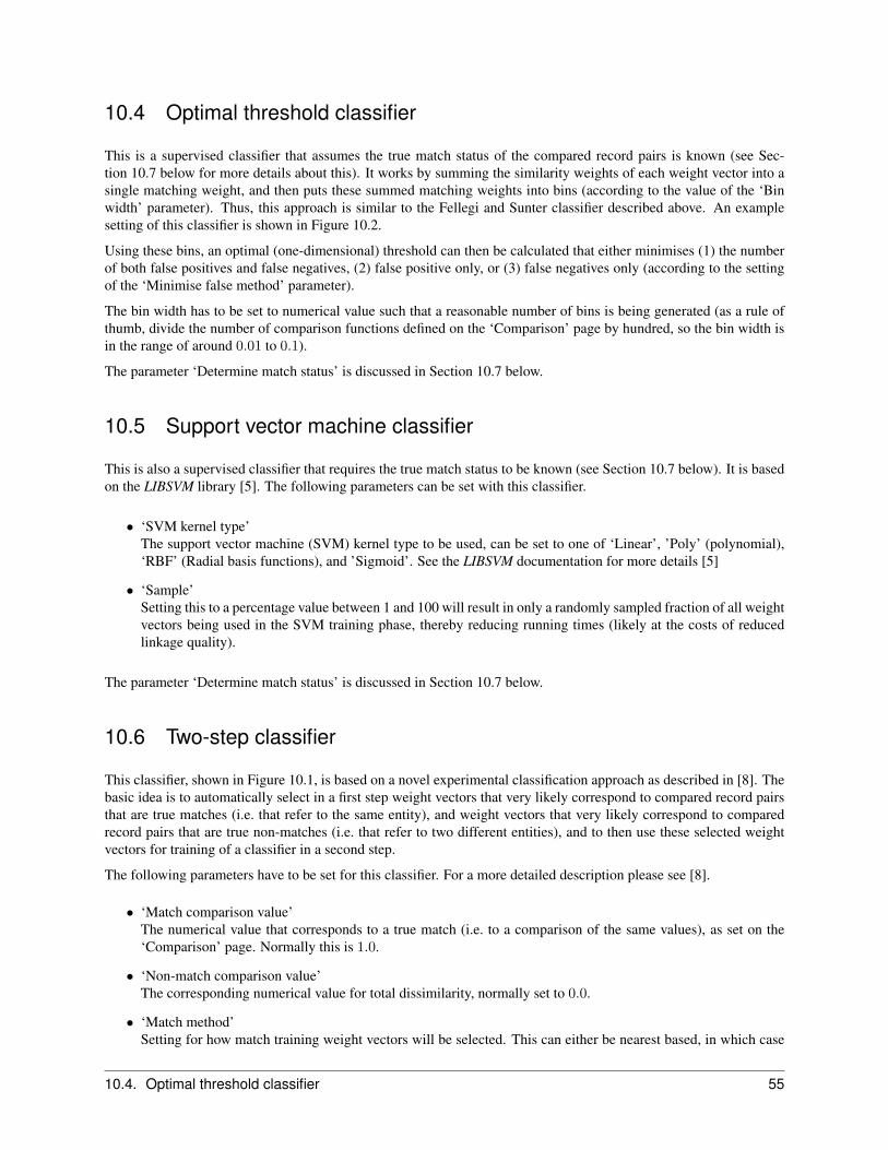
10.4 Optimal threshold classifier

This is a supervised classifier that assumes the true match status of the compared record pairs is known (see Sec-tion 10.7 below for more details about this). It works by summing the similarity weights of each weight vector into asingle matching weight, and then puts these summed matching weights into bins (according to the value of the ‘Binwidth’ parameter). Thus, this approach is similar to the Fellegi and Sunter classifier described above. An examplesetting of this classifier is shown in Figure 10.2.

Using these bins, an optimal (one-dimensional) threshold can then be calculated that either minimises (1) the numberof both false positives and false negatives, (2) false positive only, or (3) false negatives only (according to the settingof the ‘Minimise false method’ parameter).

The bin width has to be set to numerical value such that a reasonable number of bins is being generated (as a rule ofthumb, divide the number of comparison functions defined on the ‘Comparison’ page by hundred, so the bin width isin the range of around 0.01 to 0.1).

The parameter ‘Determine match status’ is discussed in Section 10.7 below.

10.5 Support vector machine classifier

This is also a supervised classifier that requires the true match status to be known (see Section 10.7 below). It is basedon the LIBSVM library [5]. The following parameters can be set with this classifier.

• ‘SVM kernel type’The support vector machine (SVM) kernel type to be used, can be set to one of ‘Linear’, ’Poly’ (polynomial),‘RBF’ (Radial basis functions), and ’Sigmoid’. See the LIBSVM documentation for more details [5]

• ‘Sample’Setting this to a percentage value between 1 and 100 will result in only a randomly sampled fraction of all weightvectors being used in the SVM training phase, thereby reducing running times (likely at the costs of reducedlinkage quality).

The parameter ‘Determine match status’ is discussed in Section 10.7 below.

10.6 Two-step classifier

This classifier, shown in Figure 10.1, is based on a novel experimental classification approach as described in [8]. Thebasic idea is to automatically select in a first step weight vectors that very likely correspond to compared record pairsthat are true matches (i.e. that refer to the same entity), and weight vectors that very likely correspond to comparedrecord pairs that are true non-matches (i.e. that refer to two different entities), and to then use these selected weightvectors for training of a classifier in a second step.

The following parameters have to be set for this classifier. For a more detailed description please see [8].

• ‘Match comparison value’The numerical value that corresponds to a true match (i.e. to a comparison of the same values), as set on the‘Comparison’ page. Normally this is 1.0.

• ‘Non-match comparison value’The corresponding numerical value for total dissimilarity, normally set to 0.0.

• ‘Match method’Setting for how match training weight vectors will be selected. This can either be nearest based, in which case

10.4. Optimal threshold classifier 55

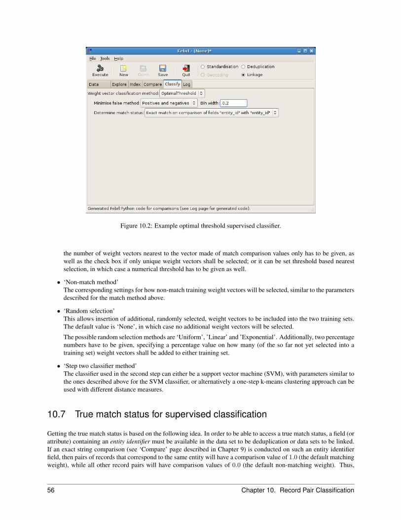
Figure 10.2: Example optimal threshold supervised classifier.

the number of weight vectors nearest to the vector made of match comparison values only has to be given, aswell as the check box if only unique weight vectors shall be selected; or it can be set threshold based nearestselection, in which case a numerical threshold has to be given as well.

• ‘Non-match method’The corresponding settings for how non-match training weight vectors will be selected, similar to the parametersdescribed for the match method above.

• ‘Random selection’This allows insertion of additional, randomly selected, weight vectors to be included into the two training sets.The default value is ‘None’, in which case no additional weight vectors will be selected.

The possible random selection methods are ‘Uniform’, ’Linear’ and ’Exponential’. Additionally, two percentagenumbers have to be given, specifying a percentage value on how many (of the so far not yet selected into atraining set) weight vectors shall be added to either training set.

• ‘Step two classifier method’The classifier used in the second step can either be a support vector machine (SVM), with parameters similar tothe ones described above for the SVM classifier, or alternatively a one-step k-means clustering approach can beused with different distance measures.

10.7 True match status for supervised classification

Getting the true match status is based on the following idea. In order to be able to access a true match status, a field (orattribute) containing an entity identifier must be available in the data set to be deduplication or data sets to be linked.If an exact string comparison (see ‘Compare’ page described in Chapter 9) is conducted on such an entity identifierfield, then pairs of records that correspond to the same entity will have a comparison value of 1.0 (the default matchingweight), while all other record pairs will have comparison values of 0.0 (the default non-matching weight). Thus,

56 Chapter 10. Record Pair Classification

record pairs with a 1.0 matching weight in this comparison correspond to true matches, and all other record pairs totrue non-matches.

Thus, all a user has to do (assuming she or he has one or two data sets containing entity identifier information) isto define an exact string comparison on the entity identifier field, and when selecting a supervised classifier (optimalthreshold or SVM), the corresponding comparison has to be selected from the drop-down list given with the parameter‘Determine match status’.

Note: The entity identifier exact string match can also be used with unsupervised classifiers for the evaluation of thededuplication or linkage quality on the ‘Evaluate’ page, as described in Chapter 12.

10.7. True match status for supervised classification 57

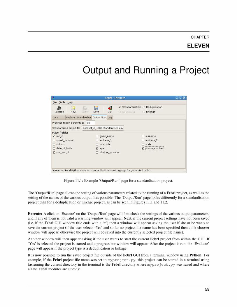
CHAPTER

ELEVEN

Output and Running a Project

Figure 11.1: Example ‘Output/Run’ page for a standardisation project.

The ‘Output/Run’ page allows the setting of various parameters related to the running of a Febrl project, as well as thesetting of the names of the various output files possible. The ‘Output/Run’ page looks differently for a standardisationproject than for a deduplication or linkage project, as can be seen in Figures 11.1 and 11.2.

Execute: A click on ‘Execute’ on the ‘Output/Run’ page will first check the settings of the various output parameters,and if any of them is not valid a warning window will appear. Next, if the current project settings have not been saved(i.e. if the Febrl GUI window title ends with a ‘*’) then a window will appear asking the user if she or he wants tosave the current project (if the user selects ‘Yes’ and so far no project file name has been specified then a file chooserwindow will appear, otherwise the project will be saved into the currently selected project file name).

Another window will then appear asking if the user wants to start the current Febrl project from within the GUI. If‘Yes’ is selected the project is started and a progress bar window will appear. After the project is run, the ‘Evaluate’page will appear if the project type is a deduplication or linkage.

It is now possible to run the saved project file outside of the Febrl GUI from a terminal window using Python. Forexample, if the Febrl project file name was set to myproject.py, this project can be started in a terminal using(assuming the current directory in the terminal is the Febrl directory where myproject.py was saved and whereall the Febrl modules are stored):

59

user@mymachine:febrlfolder> python myproject.py

11.1 Output settings for a standardisation project

Figure 11.1 shows the ‘Output/Run’ page for a standardisation project. The following parameters can be set by theuser.

• ‘Progress report percentage’This parameter determines how frequent a progress report is being reported when a Febrl standardisation projectis started from outside the GUI using Python (as described above). The value entered can be number between1 and 100 (assumed to be a percentage value), or ‘None’ (in which case no progress will be reported).

Note: When a standardisation project is started within the Febrl GUI then a progress bar is shown that will beupdated constantly, thus this parameter does not have any effect for running projects within the Febrl GUI.

• ‘Standardised output file’This has to be set to the file name of the output file that will contain the standardised version of the input data.Per default, the name is set to the name of the input data set with the string ‘-standardised’ added at the end (butbefore the file extension). A user can change this file name manually if needed.

Note: Currently, the data set type of the standardised output data set is fixed to a comma separated values(CSV) data set. This CSV data set will contain a header line with the field names in the first line. It is howeverpossible to change this in the Febrl project file generated (when the project file has been saved).

• ‘Pass fields’As can be seen in Figure 11.1, a list of all fields (attributes, columns) from the input data set will be shown, withthe possibility to check (activate) individual fields.

If a box is checked (activated) next to a field name, then the corresponding field will be written unstandardised(unmodified) from the input data set into the output data set.

For example, for the pass fields shown in Figure 11.1, the ‘rec id’, ‘soc sec id’, ‘age’ and ‘phone number’ fieldvalues will be read from the input data set and written unmodified into the output data set.

11.2 Output settings for a deduplication or linkage project

The ‘Output/Run’ page for a deduplication or linkage project is shown in Figure 11.2. The following parameters canbe set by the user.

• ‘Progress report percentage’Please see discussion above in Section 11.1 (for a standardisation project) on this parameter.

• ‘Length filtering percentage’If set to a number between 1 and 100 (assumed to be a percentage value), then in the record pair comparisonstep the length (in characters) of the record fields will be compared before the actual field comparison functionsare being executed. Length filtering is described in more details in [17].

If the percentage difference in lengths is larger than the percentage value given in this parameter, then the tworecords will not be compared but are assumed to be non-matches. The basic idea is that if two records havefields of very different lengths they will likely not refer to the same entity. For example, for two records

60 Chapter 11. Output and Running a Project

Figure 11.2: Example ‘Output/Run’ page for a linkage project.

rec1 = ‘peter paul miller canberra’rec2 = ‘joe miller sydney’

of length 26 and 17, respectively, their corresponding percentage difference will be calculated as abs(26 −17)/max(26, 17) = 9/26 = 35%. Therefore, if the length filtering percentage is set to a value smaller than35% this record pair will not be compared but directly classified as a non-match.

If no such length filtering is to be done then this parameter can be set to ‘None’ (which is the default value).

• ‘Weight vector cut-off threshold’This parameter allows filtering of compared record pairs that have a summed weight vector below the thresholdvalue given in this parameter. If this parameter is set to a value, all weight vectors that have their summedweights below this value will not be stored but are assumed to be non-matches.

The default value is ‘None’, in which case all weight vectors will be stored, classified and possibly written intoan output file.

• ‘Save weight vector file’If this check box is activated, then the corresponding file selector button will become sensitive (i.e. it can beclicked and a file name can be selected).

If activated, a weight vector file will be generated during the running of a deduplication or linkage project. Thisfile is of type comma separated values (CSV), with the first two columns being the two record identifier valuesof the pairs of records being compared, and the following columns containing the matching weights (similarityvalues) of the comparison functions defined on the ‘Comparison’ page (see Chapter 9). The total number ofcolumns in this file will therefore correspond to the number of comparison functions defined plus 2.

By default this parameter is not activated, in which case the weight vectors will not be written into a file but onlystored in memory and used in the current Febrl project.

• ‘Save histogram file’If this check box is activated and a file name is given, a simple ASCII text based histogram will be written into

11.2. Output settings for a deduplication or linkage project 61

a text file. The histogram is rotated clock-wise by 90 degrees and similar to the histogram shown in Figure 13.2on the ‘Log’ page after a deduplication or linkage project was run.

By default value this parameter is not activated and so no histogram file will be written.

• ‘Save match status file’If this check box is activated, a file of type comma separated values (CSV) is written into the file name provided.This file will contain the record identifiers and summed matching weights of the compared record pairs. It con-tains four columns, the first two being the record identifiers of the compared records, the third being the summedmatching weight (i.e. the summed similarity values of all comparison functions defined on the ‘Compare’ page,see Chapter 9), and the fourth column will contain a unique match identifier (for each matched pair of records)of the form ‘midXXXXXX’, with XXXXX being a unique number for each match (i.e. each compared recordpair). Please see Chapter 5 for more details about record identifiers and how they are used by Febrl. The fol-lowing lines show an example match status file for a linkage (where the record identifiers from the two files aredifferentiated by ‘a’ and ‘b’):

__rec_id__-0a, __rec_id__-133b, 0.555556, mid0001__rec_id__-0a, __rec_id__-180b, 0.444444, mid0002__rec_id__-0a, __rec_id__-654b, 0.444444, mid0003__rec_id__-0a, __rec_id__-895b, 0.555556, mid0004__rec_id__-0a, __rec_id__-989b, 1.000000, mid0005__rec_id__-1a, __rec_id__-458b, 1.000000, mid0006

In combination with the saved match data set(s) (see below) this file allows a generic way of processing andmerging the matches produced by a Febrl deduplication or linkage project.

• ‘Save match data set(s)’If this parameter is activated, the original input data set for a deduplication (or data sets for a linkage) will besaved into the given file name(s) with one additional field (column or attribute): the match status containingnone, one, or several match identifiers (of the form ‘midXXXXXX’ as described above) separated by semi-colons (‘;’).

The file name can be modified by the user, as can the name of the match status field (set per default to ‘match -id’).

If the record identifier field is not one of the fields in the input data set, then additionally a record identifier fieldwill be added to the output data set.

Currently the output data set(s) to be written will be of type comma separated values (CSV), with a header linewith the field names in the first line.

62 Chapter 11. Output and Running a Project

CHAPTER

TWELVE

Deduplication and Linkage Evaluation

Figure 12.1: Example linkage evaluation from a classification without known match status. Record pairs are classifiedinto matches, non-matches and possible matches.

The ‘Evaluation’ page visualises the results of a deduplication or linkage project as a histogram of the summed weightvectors, i.e. the numerical similarity values of all comparisons defined on the ‘Comparison’ page (see Chapter 9) aresummed for each compared record pair, and a histogram is generated as shown in Figures 12.1 and 12.2. Dependingupon if the true match status is available for a deduplication or linkage, either only the matches, non-matches andpossible matches can be shown, or (with known match status) also the number of matches and non-matches that wereclassified true or false. Additionally, deduplication or linkage quality and complexity measures are calculated andshown below the histogram.

If the true match status of the compared record pairs is not known, only the reduction ratio measure can be calculated,as all other measures require the true match status. In case the true match status is available, the quality measurespresented below are calculated. For a more detailed discussion of the issues involved in measuring linkage quality andcomplexity please see [10].

For the following quality measures it is assumed that TP is the number of true matches (true positives), FP thenumber of false matches (false positives, i.e. true non-matches that were classified as matches), TN the number of

63

Figure 12.2: Example linkage evaluation from a classification with known match status. Record pairs are classifiedinto matches and non-matches (with true and false matches, and true and false non-matches shown).

true non-matches (true negatives), and FN the number of false non-matches (false negatives, i.e. true matches thatwere classified as non-matches).

• Accuracy is measured as: acc = TP+TNTP+FP+TN+FN .

• Precision (also called the positive predictive value) is measured as: prec = TPTP+FP .

• Recall (the true positive rate, also known as sensitivity) is measured as: rec = TPTP+FN .

• F-measure (or F-score) is the harmonic mean of precision and recall and is calculated as:f−meas = 2(prec×rec

prec+rec ).

Note: The accuracy measure commonly used in machine learning applications is often misleading in record linkageapplications due to the large number of non-matches compared to matches [10], i.e. classifying record pairs is oftena very imbalanced classification problem. Accuracy is shown on the Febrl GUI to allow users to learn about itsmisleading characteristic, as well as to compare quality measure results.

For the linkage complexity measures, following [7, 13], let nM and nU be the total number of matched and un-matchedrecord pairs, respectively, such that (nM + nU ) = |A| × |B| (with | · | denoting the number of records in a database)for linkage of two databases A and B. Next, let sM and sU be the number of true matched and true non-matchedrecord pairs generated by a blocking technique, respectively, with (sM + sU ) (nM + nU ).

• Reduction ratio is measured as: rr = 1.0− (sM+sU )(nM+nU ) .

• Pairs completeness is measured as: pc = sM

nM.

• Pairs quality is measured as: pq = sM

(sM+sU ) .

Note: As can be seen from Figures 12.1 and 12.2, the ‘Execute’ button is not sensitive on the ‘Evaluate’ page, as noinitialisation of settings or execution of code can be done on this page.

64 Chapter 12. Deduplication and Linkage Evaluation

CHAPTER

THIRTEEN

Log Page

Figure 13.1: Example ‘Log’ page showing the Febrl code generated for the indexing example shown in Figure 8.1.

On the ‘Log’ page the user can view the Febrl code segments that were generated when the ‘Execute’ button wasclicked on the various other Febrl GUI pages. Figure 13.1, for example, shows the code that was generated when the‘SortingIndex’ (using the ‘DedupIndex’ implementation) with window size 3 from Figure 8.1 was initialised.

An experienced Febrl user can visually validate the generated Febrl code on the ‘Log’ page, but also copy-paste thiscode into her or his own Febrl project files (and manually modify it if required), or copy the generated code into anexisting Febrl project file (for example to change the indexing techniques used for a project).

After a deduplication or linkage project has been run from the ‘Output/Run’ page, detailed information about theproduced linkage (number of matches, non-matches and possible matches) and a simple textual histogram representingthe summed matching weights will be shown in the ‘Log’ page, as can be seen in Figure 13.2. In case of supervisedclassification (see Chapter 10) the classification results will also be shown.

65

Figure 13.2: Example ‘Log’ page showing the weight vector histogram and linkage quality as generated with thesupervised classifier shown in Figure 10.1.

Note: As can be seen from Figures 13.1 and 13.2, the ‘Execute’ button is not sensitive on the ‘Log’ page, as noinitialisation of settings or execution of code can be done on this page.

66 Chapter 13. Log Page

APPENDIX

A

Installation

Warning: Febrl, including its graphical user interface, has been developed and tested on a Linux platform(Ubuntu version 7.04). The author has only very limited experience with installing Python and additional librarieson other platforms.Any detailed instructions and help on installing Febrl on various platforms, as well as reports on problems en-countered during installation, are much appreciated (please e-mail the author).

A.1 Installation on Linux/Unix

The packages required on Linux system include Python (version 2.5), PyGTK, Numpy, Matplotlib, and LIBSVM.Please see page i (‘See also’ section) for the URLs from where more detailed information about these programs andlibraries is available. It is assumed that these libraries have been installed on the system where Febrl will be installed.

To test if the required modules are installed properly, start Python from a terminal (console) window, and try to importthe following five modules:

user@mymachine:anyfolder> python>>> import pygtk>>> import pygtk.glade>>> import numpy>>> import matplotlib>>> import svm

If you receive an error message with any of these imports, or if you cannot start Python you have to install the requiredpackages. This might have to be done by a system administrator if you do not have the access rights to install systempackages.

A.1.1 Unpacking and installation of Febrl

Unpack the febrl-0.4.tar.gz or febrl-0.4.zip archive and a new directory named ‘febrl-0.4’ will be created con-taining all the necessary Febrl modules and additional files such as example data sets, documentation, the Febrl dataset generator, as well as testing programs. To unpack, use either:

user@mymachine:febrlfolder> gunzip febrl-0.4.tar.gzuser@mymachine:febrlfolder> tar xvf febrl-0.4.tar

or:

67

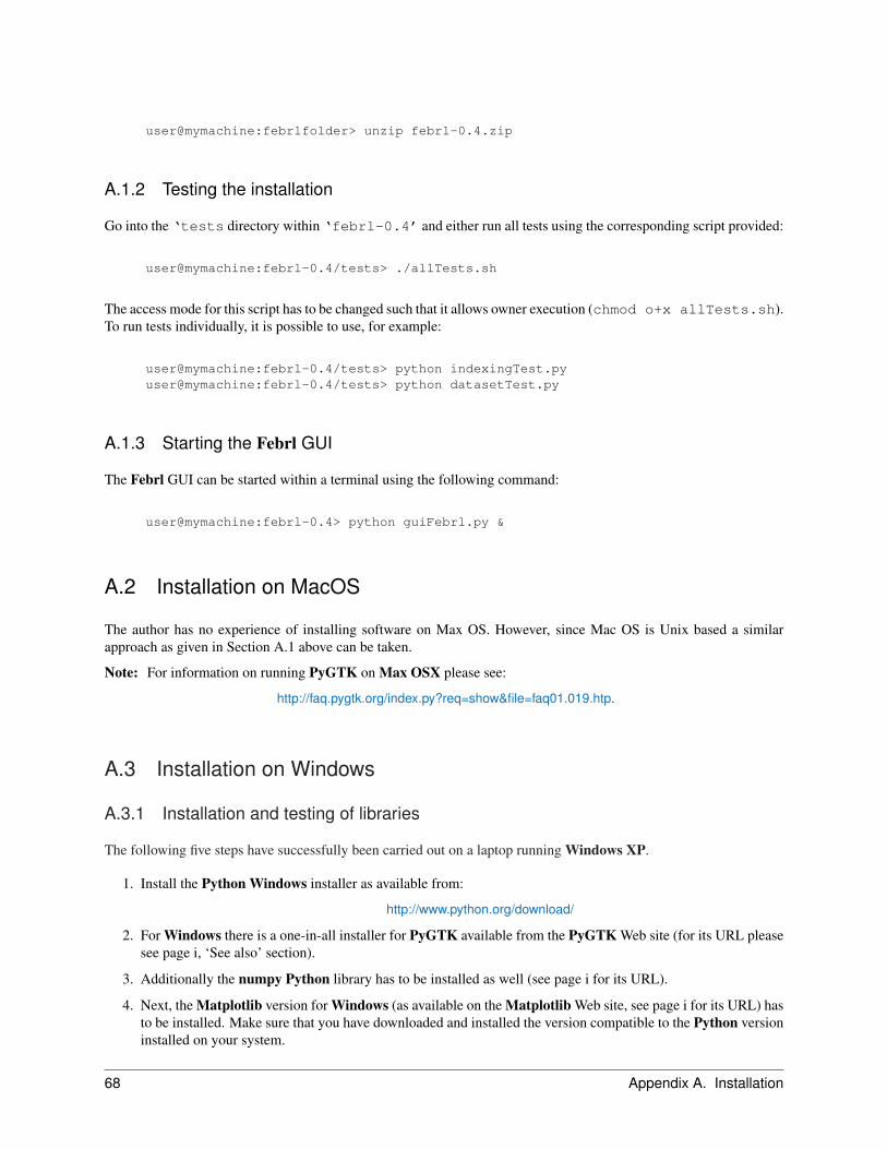
user@mymachine:febrlfolder> unzip febrl-0.4.zip

A.1.2 Testing the installation

Go into the ‘tests directory within ‘febrl-0.4’ and either run all tests using the corresponding script provided:

user@mymachine:febrl-0.4/tests> ./allTests.sh

The access mode for this script has to be changed such that it allows owner execution (chmod o+x allTests.sh).To run tests individually, it is possible to use, for example:

user@mymachine:febrl-0.4/tests> python indexingTest.pyuser@mymachine:febrl-0.4/tests> python datasetTest.py

A.1.3 Starting the Febrl GUI

The Febrl GUI can be started within a terminal using the following command:

user@mymachine:febrl-0.4> python guiFebrl.py &

A.2 Installation on MacOS

The author has no experience of installing software on Max OS. However, since Mac OS is Unix based a similarapproach as given in Section A.1 above can be taken.

Note: For information on running PyGTK on Max OSX please see:

http://faq.pygtk.org/index.py?req=show&file=faq01.019.htp.

A.3 Installation on Windows

A.3.1 Installation and testing of libraries

The following five steps have successfully been carried out on a laptop running Windows XP.

1. Install the Python Windows installer as available from:

http://www.python.org/download/

2. For Windows there is a one-in-all installer for PyGTK available from the PyGTK Web site (for its URL pleasesee page i, ‘See also’ section).

3. Additionally the numpy Python library has to be installed as well (see page i for its URL).

4. Next, the Matplotlib version for Windows (as available on the Matplotlib Web site, see page i for its URL) hasto be installed. Make sure that you have downloaded and installed the version compatible to the Python versioninstalled on your system.

68 Appendix A. Installation

http://faq.pygtk.org/index.py?req=show&file=faq01.019.htp

http://www.python.org/download/

5. The LIBSVM library can be downloaded from the Web site given on page i, which also includes instructionon how to install the Python LIBSVM library. On a Windows XP laptop, assuming standard installation, theLIBSVM files from the folder python and windows/python had to be copied into the folder:

C:\\Program Files\PyGTK\Python\LIB\site-packagesThis might be different on other Windows versions.

To test if the required modules are installed properly, start Python (command line) from the Programs → Python2.X menu, and try to load the following five modules:

>>>> import pygtk>>>> import pygtk.glade>>>> import numpy>>>> import matplotlib>>>> import svm

A.3.2 Unpacking, installation and starting of Febrl

Unpack the febrl-0.4.zip archive and a new directory named ‘febrl-0.4’ will be created. It should now bepossible to start the Febrl GUI with a double-click on the GuiFebrl module. A terminal window and the Febrl GUIwill appear.

A.3. Installation on Windows 69

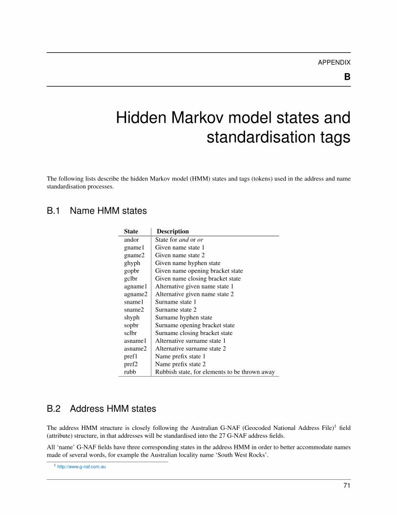
APPENDIX

B

Hidden Markov model states andstandardisation tags

The following lists describe the hidden Markov model (HMM) states and tags (tokens) used in the address and namestandardisation processes.

B.1 Name HMM states

State Descriptionandor State for and or orgname1 Given name state 1gname2 Given name state 2ghyph Given name hyphen stategopbr Given name opening bracket stategclbr Given name closing bracket stateagname1 Alternative given name state 1agname2 Alternative given name state 2sname1 Surname state 1sname2 Surname state 2shyph Surname hyphen statesopbr Surname opening bracket statesclbr Surname closing bracket stateasname1 Alternative surname state 1asname2 Alternative surname state 2pref1 Name prefix state 1pref2 Name prefix state 2rubb Rubbish state, for elements to be thrown away

B.2 Address HMM states

The address HMM structure is closely following the Australian G-NAF (Geocoded National Address File)1 field(attribute) structure, in that addresses will be standardised into the 27 G-NAF address fields.

All ‘name’ G-NAF fields have three corresponding states in the address HMM in order to better accommodate namesmade of several words, for example the Australian locality name ‘South West Rocks’.

1 http://www.g-naf.com.au

71

http://www.g-naf.com.au

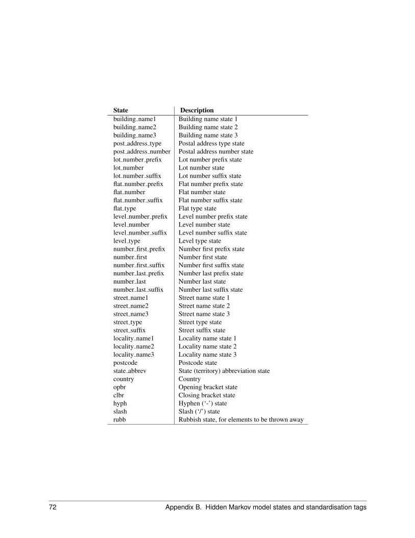
State Descriptionbuilding name1 Building name state 1building name2 Building name state 2building name3 Building name state 3post address type Postal address type statepost address number Postal address number statelot number prefix Lot number prefix statelot number Lot number statelot number suffix Lot number suffix stateflat number prefix Flat number prefix stateflat number Flat number stateflat number suffix Flat number suffix stateflat type Flat type statelevel number prefix Level number prefix statelevel number Level number statelevel number suffix Level number suffix statelevel type Level type statenumber first prefix Number first prefix statenumber first Number first statenumber first suffix Number first suffix statenumber last prefix Number last prefix statenumber last Number last statenumber last suffix Number last suffix statestreet name1 Street name state 1street name2 Street name state 2street name3 Street name state 3street type Street type statestreet suffix Street suffix statelocality name1 Locality name state 1locality name2 Locality name state 2locality name3 Locality name state 3postcode Postcode statestate abbrev State (territory) abbreviation statecountry Countryopbr Opening bracket stateclbr Closing bracket statehyph Hyphen (‘-’) stateslash Slash (‘/’) staterubb Rubbish state, for elements to be thrown away

72 Appendix B. Hidden Markov model states and standardisation tags

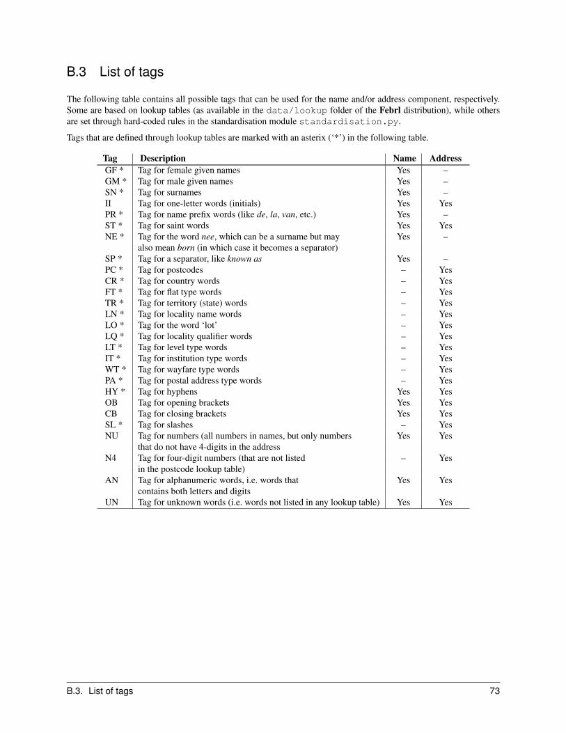
B.3 List of tags

The following table contains all possible tags that can be used for the name and/or address component, respectively.Some are based on lookup tables (as available in the data/lookup folder of the Febrl distribution), while othersare set through hard-coded rules in the standardisation module standardisation.py.

Tags that are defined through lookup tables are marked with an asterix (‘*’) in the following table.

Tag Description Name AddressGF * Tag for female given names Yes –GM * Tag for male given names Yes –SN * Tag for surnames Yes –II Tag for one-letter words (initials) Yes YesPR * Tag for name prefix words (like de, la, van, etc.) Yes –ST * Tag for saint words Yes YesNE * Tag for the word nee, which can be a surname but may Yes –

also mean born (in which case it becomes a separator)SP * Tag for a separator, like known as Yes –PC * Tag for postcodes – YesCR * Tag for country words – YesFT * Tag for flat type words – YesTR * Tag for territory (state) words – YesLN * Tag for locality name words – YesLO * Tag for the word ‘lot’ – YesLQ * Tag for locality qualifier words – YesLT * Tag for level type words – YesIT * Tag for institution type words – YesWT * Tag for wayfare type words – YesPA * Tag for postal address type words – YesHY * Tag for hyphens Yes YesOB Tag for opening brackets Yes YesCB Tag for closing brackets Yes YesSL * Tag for slashes – YesNU Tag for numbers (all numbers in names, but only numbers Yes Yes

that do not have 4-digits in the addressN4 Tag for four-digit numbers (that are not listed – Yes

in the postcode lookup table)AN Tag for alphanumeric words, i.e. words that Yes Yes

contains both letters and digitsUN Tag for unknown words (i.e. words not listed in any lookup table) Yes Yes

B.3. List of tags 73

APPENDIX

C

To-Do: Outstanding Development Tasks,Possible Additions and Enhancements

This is an incomplete list of outstanding development tasks and possible additions and enhancements to the Febrlsystem.

The first part contains things to-do on the Febrl GUI, while the second part contains to-do’s for the various Febrlmodules.

Febrl GUI:----------

- Load and parse a Febrl project file

- possibility to show/edit the generated code??

- implement data set generator as extra tool as separate window

- implement HMM training in GUI as extra tool

Data page:

Explore page:

Indexing page:- scrolling down automatically in index definition window

Comparison page:- comparisons: fields re-set (clear) when change, improve upon this- add frequency based weight calculation (i.e. load freq. files)

Classify:

Output/Run:

Evaluate:- add interactive threshold setting

Review:- implement Review page

75

General Febrl modules:----------------------

- dataset.py:- SQL data set classes and their tests in datasetTest.py

- comparisonTest.py:- more test on caching- proper timing analysis of comparison functions (incl. caching)using large data sets

- measurements.py- check improve pairs completeness - is rec_id funct needed?- implement measurementsTest.py

- indexing.py- add test in indexingTest.py writing of weight vector file

- output.py:- add more output options (merged linked data sets?)- implement outputTest.py

- classification.py- add log_funct to classification for progress reporting

- various clustering quality measuresthen k-means with k=2,3... keep best K

- improve decision tree classifier, e.g. C4.5 in C? Similar to SVM- hierarchical agglomerative clustering, add [1,1,1,1]weight vector (all matches) and [0,0,0,0] non-matches -> 2 knownclusters, then find next closest etc. -> down to 2 clusters.

- have classifiers all with a vector_weight argument which givesdifferent weights to fields in vectors, if None -> all weight 1.0

- mymath.py:- finalise Mahalanobis distance- update mymathTest.py

- standardise.py- complete names and address testing routines in standardiseTest.py

- stringcmp.py- improve compression comparison-> module compression with different algorithms

- lap.py- fix LAP module, then test- update to Python 2.5, integrate into Febrl-0.4

76 Appendix C. To-Do: Outstanding Development Tasks, Possible Additions and Enhancements

APPENDIX

D

Version History

0.1 First public release (6 September 2002)Modules for data cleaning and standardisation, hidden Markov model (HMM) training.

0.2 Second public release (14 April 2003)Complete object-oriented re-design, includes modules for probabilistic linkage.

0.2.1 Updated second public release (26 June 2003)This version is published under an updated ANUOS license version 1.1. Added top level rou-tine standardise in module febrl, added the flexible classifier in module linkage, added aPassFieldStandardiserwhich allows simple passing of fields without standardisation, added the data setgenerator generate.py, added improved one-to-one assignment based on Auction [4] algorithm, improvedmemory management and verbose output, added process indicators, added Berkeley database library support inShelve data set, plus many smaller improvements and bug fixes.

0.2.2 Bug-fix release (November 2003)This is a bug-fix release for Febrl 0.2.1. Thanks to everybody who sent us bug reports. The manual is nowprocessed using the Python 2.3.2 documentation system.

0.3 Third public release (April 2005)Includes a geocoding matching system based on the Australian G-NAF (Geocoded National Address File)database. Various smaller additions, including several new field comparison functions, a telephone numberstandardiser, CSV (comma separated values) output of the linkage results, and a new logging system based onthe standard Python logging module. Updated all modules to Python 2.4.

0.4 Fourth public release (November 2007)Includes a graphical user interface (GUI), a completely redesigned module structure, many new field comparisonfunctions, several new indexing (blocking) techniques and classification approaches. Updated to Python 2.5.Completely rewritten manual.

0.4.01 Fifth public release (December 2007)This is a bug-fix release for Febrl 0.4. No new features were added, but several smaller bugs and inconsistencieswere cleaned up. Additionally, a new chapter was added to the Manual, containing two tutorials.

0.4.02 Sixth public release (April 2008)This is another bug fix release for Febrl 0.4. It does not contain new features but several bugs in the main Febrlmodules were fixed.

0.4.1 Seventh public release (December 2008)This is another bug fix release for Febrl 0.4. It does not contain new features in the main Febrl programmodules, but it does include a much improved new data set generator (dsgen2) which allows more accurate datageneration, enables attribute dependencies, and also facilitates the generation of family and household data.

77

APPENDIX

E

Support Arrangements

As stated in the License (see Appendix F), Febrl is provided on an AS IS basis, WITHOUT WARRANTY OF ANYKIND, either expressed or implied.

However, the authors are keen to learn of any bugs, defects or limitations in the software. At this stage, just e-mail thedetails to the authors (see title page of this manual).

Two mailing lists have been set up at Sourceforge.Net1. For more details see

https://sourceforge.net/mail/?group id=62161

If you are interested in this project please subscribe and we will inform you of software releases, publications andother output of this project.

Users or potential users of Febrl should note that although problems with the programs will be attended to on a besteffort basis, the authors have other responsibilities (not to mention families and friends) and do not undertake to resolveproblems within any particular time frame, or at all, as the case may be. Because the source code for Febrl is freelyavailable, users may be able to resolve many problems themselves, or with the help of others who have experiencewith the Python programming language. We would appreciate it if copies of such fixes and modifications are e-mailedto us so that they can be incorporated into future versions of Febrl.

1 http://sourceforge.net

79

https://sourceforge.net/mail/?groupunhbox voidb@x penalty @M hskip z@skip unhbox voidb@x kern .06emvbox hrule width.3emdiscretionary -penalty @M hskip z@skip id=62161

http://sourceforge.net

APPENDIX

F

ANU – Open Source License

AUSTRALIAN NATIONAL UNIVERSITYOPEN SOURCE LICENSE (ANUOS LICENSE)

VERSION 1.31. DEFINITIONS

Associated Documentation and Data Files shall mean all files distributed in conjunction with the Original Software which are notcomputer program code.

Commercial Use shall mean distribution or otherwise making the Covered Software available to a third party.

Contributor shall mean each entity that creates or contributes to the creation of Modifications.

Contributor Version shall mean in case of any Contributor the combination of the Original Software, prior Modifications used by aContributor, and the Modifications made by that particular Contributor and in case of the Australian National University in additionthe Original Software in any form, including the form as Executable.

Covered Software shall mean the Original Software and Associated Documentation and Data Files or Modifications or the combi-nation of the Original Software and Associated Documentation and Data Files and Modifications, in each case including portionsthereof.

Electronic Distribution Mechanism shall mean a mechanism generally accepted in the software development community for theelectronic transfer of data.

Executable shall mean Covered Software in any form other than Source Code.

Initial Developer shall mean the individual or entity identified as the Initial Developer in the Source Code notice required by ExhibitA.

The Australian National University shall mean the Australian National University, ABN 52-234-063-906, a body corporate pursuantto the Australian National University Act 1991 of Canberra, in the Australian Capital Territory.

Larger Work shall mean a work, which combines Covered Software or portions thereof with code not governed by the terms of thisLicense.

License shall mean this document.

Licensable shall mean having the right to grant, to the maximum extent possible, whether at the time of the initial grant or subse-quently acquired, any and all of the rights conveyed herein.

Modifications shall mean any addition to or deletion from the substance or structure of either the Original Software, the AssociatedDocumentation and Data Files or any previous Modifications. When Covered Software is released as a series of files, a Modificationis:a) Any addition to or deletion from the contents of a file containing Original Software, Associated Documentation and Data Files orprevious Modifications.b) Any new file that contains any part of the Original Software, Associated Documentation and Data Files or previous Modifications.

Original Software shall mean the Source Code of computer software code which is described in the Source Code notice required byExhibit A as Original Software, and which, at the time of its release under this License is not already Covered Software governed bythis License.

Patent Claims shall mean any patent claim(s), now owned or hereafter acquired, including without limitation, method, process, andapparatus claims, in any patent Licensable by grantor.

Source Code shall mean the preferred form of the Covered Software for making modifications to it, including all modules it contains,plus any associated interface definition files, scripts used to control compilation and installation of an Executable, or source codedifferential comparisons against either the Original Software or another well known, available Covered Software of the Contributor’schoice. The Source Code can be in a compressed or archival form, provided the appropriate decompression or de-archiving softwareis widely available for no charge.

81

You (or Your) shall mean an individual or a legal entity exercising rights under, and complying with all of the terms of, this Licenseor a future version of this License issued under Section 6.1. For legal entities, You includes an entity which controls, is controlled by,or is under common control with You. For the purposes of this definition, control means (a) the power, direct or indirect, to cause thedirection or management of such entity, whether by contract or otherwise, or (b) ownership of more than fifty per cent (50%) of theoutstanding shares or beneficial ownership of such entity.

2. SOURCE CODE LICENSE

2.1 The Australian National University Grant.Subject to the terms of this License, the Australian National University hereby grants You a world-wide, royalty-free, non-exclusivelicense, subject to third party intellectual property claims:a) under copyrights Licensable by the Australian National University to use, reproduce, modify, display, perform, sublicense anddistribute the Original Software (or portions thereof) with or without Modifications, and/or as part of a Larger Work;b) and under Patents Claims infringed by the making, using or selling of Original Software, to make, have made, use, practice, sell,and offer for sale, and/or otherwise dispose of the Original Software (or portions thereof).c) The licenses granted in this Section 2.1(a) and (b) are effective on the date the Australian National University first distributesOriginal Software under the terms of this License.d) Notwithstanding Section 2.1(b) above, no patent license is granted:1) for code that You delete from the Original Software;2) separate from the Original Software; or3) for infringements caused by: i) the modification of the Original Software or ii) the combination of the Original Software withother software or devices.

2.2 Contributor Grant.Subject to the terms of this License and subject to third party intellectual property claims, each Contributor hereby grants You aworld-wide, royalty-free, non-exclusive license:a) under copyrights Licensable by Contributor, to use, reproduce, modify, display, perform, sublicense and distribute the Modifica-tions created by such Contributor (or portions thereof) either on an unmodified basis, with other Modifications, as Covered Softwareand/or as part of a Larger Work; andb) under Patent Claims necessarily infringed by the making, using, or selling of Modifications made by that Contributor either aloneand/or in combination with its Contributor Version (or portions of such combination), to make, use, sell, offer for sale, have made,and/or otherwise dispose of:1) Modifications made by thatContributor (or portions thereof); and2) the combination of Modifications made by that Contributor with its Contributor Version (or portions of such combination).c) The licenses granted in Sections 2.2(a) and 2.2(b) are effective on the date Contributor first makes Commercial Use of the CoveredSoftware.d) Notwithstanding Section 2.2(b) above, no patent license is granted:1) for any code that Contributor has deleted from the Contributor Version;2) separate from the Contributor Version; 3) for infringements caused by: i) third party modifications of Contributor Version or ii)the combination of Modifications made by that Contributor with other software (except as part of the Contributor Version) or otherdevices; or4) under Patent Claims infringed by Covered Software in the absence of Modifications made by that Contributor.

3. DISTRIBUTION OBLIGATIONS

3.1 Application of LicenseThe Modifications which You create or to which You contribute are governed by the terms of this License, including without limitationSection 2.2. The Source Code version of Covered Software may be distributed only under the terms of this License or a future versionof this License released under Section 6.1, and You must include a copy of this License with every copy of the Source Code Youdistribute. You may not offer or impose any terms on any Source Code version that alters or restricts the applicable version of thisLicense or the recipients’ rights hereunder.

3.2 Availability of Source CodeAny Modification which You create or to which You contribute must be made available in Source Code form under the terms of thisLicense either on the same media as an Executable version or via an accepted Electronic Distribution Mechanism to anyone to whomyou made an Executable version available; and if made available via Electronic Distribution Mechanism, must remain available forat least twelve (12) months after the date it initially became available, or at least six (6) months after a subsequent version of thatparticular Modification has been made available to such recipients. You are responsible for ensuring that the Source Code versionremains available even if the Electronic Distribution Mechanism is maintained by a third party.

3.3 Description of ModificationsYou must cause all Covered Software to which You contribute to contain a file documenting the changes You made to create thatCovered Software and the date of any change. You must include a prominent statement that the Modification is derived, directly orindirectly, from Original Software provided by the Australian National University and including the name of the Australian NationalUniversity in (a) the Source Code, and (b) in any notice in an Executable version or related documentation in which You describe theorigin or ownership of the Covered Software.

82 Appendix F. ANU – Open Source License

3.4 Intellectual Property Mattersa) Third Party ClaimsIf Contributor has knowledge that a license under a third party’s intellectual property rights is required to exercise the rights grantedby such Contributor under Sections 2.1 or 2.2, Contributor must include a text file with the Source Code distribution titled ”LE-GAL” which describes the claim and the party making the claim in sufficient detail that a recipient will know whom to contact. IfContributor obtains such knowledge after the Modification is made available as described in Section 3.2, Contributor shall promptlymodify the LEGAL file in all copies Contributor makes available thereafter and shall take other steps (such as notifying appropriatemailing lists or newsgroups) reasonably calculated to inform those who received the Covered Software that new knowledge has beenobtained.b) Contributor APIsIf Contributor’s Modifications include an application programming interface (API) and Contributor has knowledge of patent licenseswhich are reasonably necessary to implement that API, Contributor must also include this information in the LEGAL file.c) RepresentationsContributor represents that, except as disclosed pursuant to Section 3.4(a) above, Contributor believes that Contributor’s Modifica-tions are Contributor’s original creation(s) and/or Contributor has sufficient rights to grant the rights conveyed by this License.

3.5 Required NoticesYou must duplicate the notice in Exhibit A in each file of the Source Code. If it is not possible to put such notice in a particularSource Code file due to its structure, then You must include such notice in a location (such as a relevant directory) where a userwould be likely to look for such a notice. If You created one or more Modification(s) You may add your name as a Contributor to thenotice described in Exhibit A. You must also duplicate this License in any documentation for the Source Code where You describerecipients’ rights or ownership rights relating to Covered Software. You may choose to offer, and to charge a fee for, warranty,support, indemnity or liability obligations to one or more recipients of Covered Software. However, You may do so only on Yourown behalf, and not on behalf of the Australian National University or any Contributor. You must make it absolutely clear that anysuch warranty, support, indemnity or liability obligation is offered by You alone, and You hereby agree to indemnify the AustralianNational University and every Contributor for any liability incurred by the Australian National University or such Contributor as aresult of warranty, support, indemnity or liability terms You offer.

3.6 Distribution of Executable VersionsYou may distribute Covered Software in Executable form only if the requirements of Sections 3.1-3.5 have been met for that CoveredSoftware, and if You include a notice stating that the Source Code version of the Covered Software is available under the terms of thisLicense, including a description of how and where You have fulfilled the obligations of Section 3.2. The notice must be conspicuouslyincluded in any notice in an Executable version, related documentation or collateral in which You describe recipients’ rights relatingto the Covered Software. You may distribute the Executable version of Covered Software or ownership rights under a license of Yourchoice, which may contain terms different from this License, provided that You are in compliance with the terms of this License andthat the license for the Executable version does not attempt to limit or alter the recipient’s rights in the Source Code version from therights set forth in this License. If You distribute the Executable version under a different license You must make it absolutely clearthat any terms which differ from this License are offered by You alone, not by the Australian National University or any Contributor.You hereby agree to indemnify the Australian National University and every Contributor for any liability incurred by the AustralianNational University or such Contributor as a result of any such terms You offer.

3.7 Larger WorksYou may create a Larger Work by combining Covered Software with other software not governed by the terms of this License anddistribute the Larger Work as a single product. In such a case, You must make sure the requirements of this License are fulfilled forthe Covered Software.

4. INABILITY TO COMPLY DUE TO STATUTE OR REGULATIONIf it is impossible for You to comply with any of the terms of this License with respect to some or all of the Covered Software due to statute,judicial order, or regulation then You must: (a) comply with the terms of this License to the maximum extent possible; and (b) describe thelimitations and the code they affect. Such description must be included in the LEGAL file described in Section 3.4 and must be includedwith all distributions of the Source Code. Except to the extent prohibited by statute or regulation, such description must be sufficientlydetailed for a recipient of ordinary skill to be able to understand it.

5. APPLICATION OF THIS LICENSEThis License applies to code to which the Australian National University has attached the notice in Exhibit A and to related CoveredSoftware.

6. VERSIONS OF THE LICENSE

6.1 New VersionsThe Australian National University may publish revised and/or new versions of the License from time to time. Each version will begiven a distinguishing version number.

6.2 Effect of New VersionsOnce Covered Software has been published under a particular version of the License, You may always continue to use it under theterms of that version. You may also choose to use such Covered Software under the terms of any subsequent version of the Licensepublished by the Australian National University. No one other than the Australian National University has the right to modify theterms applicable to Covered Software created under this License.

7. DISCLAIMER OF WARRANTYCOVERED SOFTWARE IS PROVIDED UNDER THIS LICENSE ON AN ”AS IS” BASIS, WITHOUT WARRANTY OF ANY KIND,EITHER EXPRESSED OR IMPLIED, INCLUDING, WITHOUT LIMITATION, WARRANTIES THAT THE COVERED SOFTWARE ISFREE OF DEFECTS, MERCHANTABLE, FIT FOR A PARTICULAR PURPOSE OR NON-INFRINGING. THE ENTIRE RISK AS TO

83

THE QUALITY AND PERFORMANCE OF THE COVERED SOFTWARE IS WITH YOU. SHOULD ANY COVERED SOFTWAREPROVE DEFECTIVE IN ANY RESPECT, YOU (NOT THE AUSTRALIAN NATIONAL UNIVERSITY, ITS LICENSORS OR AFFIL-IATES OR ANY OTHER CONTRIBUTOR) ASSUME THE COST OF ANY NECESSARY SERVICING, REPAIR OR CORRECTION.THIS DISCLAIMER OF WARRANTY CONSTITUTES AN ESSENTIAL PART OF THIS LICENSE. NO USE OF ANY COVEREDSOFTWARE IS AUTHORIZED HEREUNDER EXCEPT UNDER THIS DISCLAIMER.

8. TERMINATION

8.1 This License and the rights granted hereunder will terminate automatically if You fail to comply with terms herein and fail to curesuch breach within 30 days of becoming aware of the breach. All sublicenses to the Covered Software which are properly grantedshall survive any termination of this License. Provisions which, by their nature, must remain in effect beyond the termination of thisLicense shall survive.

8.2 If You initiate litigation by asserting a patent infringement claim (excluding declatory judgment actions) against the AustralianNational University or a Contributor (the Australian National University or Contributor against whom You file such action is referredto as ”Participant”) alleging that:a) such Participant’s Contributor Version directly or indirectly infringes any patent, then any and all rights granted by such Participantto You under Sections 2.1 and/or 2.2 of this License shall, upon 60 days notice from Participant terminate prospectively, unless ifwithin 60 days after receipt of notice You either: (i) agree in writing to pay Participant a mutually agreeable reasonable royaltyfor Your past and future use of Modifications made by such Participant, or (ii) withdraw Your litigation claim with respect to theContributor Version against such Participant. If within 60 days of notice, a reasonable royalty and payment arrangement are notmutually agreed upon in writing by the parties or the litigation claim is not withdrawn, the rights granted by Participant to You underSections 2.1 and/or 2.2 automatically terminate at the expiration of the 60 day notice period specified above.b) any software, hardware, or device, other than such Participant’s Contributor Version, directly or indirectly infringes any patent,then any rights granted to You by such Participant under Sections 2.1(b) and 2.2(b) are revoked effective as of the date You first made,used, sold, distributed, or had made, Modifications made by that Participant.

8.3 If You assert a patent infringement claim against Participant alleging that such Participant’s Contributor Version directly or indirectlyinfringes any patent where such claim is resolved (such as by license or settlement) prior to the initiation of patent infringementlitigation, then the reasonable value of the licenses granted by such Participant under Sections 2.1 or 2.2 shall be taken into accountin determining the amount or value of any payment or license.

8.4 In the event of termination under Sections 8.1 or 8.2 above, all end user license agreements (excluding distributors and resellers)which have been validly granted by You or any distributor hereunder prior to termination shall survive termination.

9. LIMITATION OF LIABILITYUNDER NO CIRCUMSTANCES AND UNDER NO LEGAL THEORY, WHETHER TORT (INCLUDING NEGLIGENCE), CON-TRACT, OR OTHERWISE, SHALL YOU, THE AUSTRALIAN NATIONAL UNIVERSITY, ANY OTHER CONTRIBUTOR, OR ANYDISTRIBUTOR OF COVERED SOFTWARE, OR ANY SUPPLIER OF ANY OF SUCH PARTIES, BE LIABLE TO ANY PERSONFOR ANY INDIRECT, SPECIAL, INCIDENTAL, OR CONSEQUENTIAL DAMAGES OF ANY CHARACTER INCLUDING, WITH-OUT LIMITATION, DAMAGES FOR LOSS OF GOODWILL, WORK STOPPAGE, COMPUTER FAILURE OR MALFUNCTION, ORANY AND ALL OTHER COMMERCIAL DAMAGES OR LOSSES, EVEN IF SUCH PARTY SHALL HAVE BEEN INFORMED OFTHE POSSIBILITY OF SUCH DAMAGES. THIS LIMITATION OF LIABILITY SHALL NOT APPLY TO LIABILITY FOR DEATHOR PERSONAL INJURY RESULTING FROM SUCH PARTY’S NEGLIGENCE TO THE EXTENT APPLICABLE LAW PROHIBITSSUCH LIMITATION. SOME JURISDICTIONS DO NOT ALLOW THE EXCLUSION OR LIMITATION OF INCIDENTAL OR CON-SEQUENTIAL DAMAGES, BUT MAY ALLOW LIABILITY TO BE LIMITED; IN SUCH CASES, A PARTY’S, ITS EMPLOYEES’,LICENSORS’ OR AFFILIATES’ LIABILITY SHALL BE LIMITED TO AUD $100. NOTHING CONTAINED IN THIS LICENSESHALL PREJUDICE THE STATUTORY RIGHTS OF ANY PARTY DEALING AS A CONSUMER.

10. MISCELLANEOUS. This License represents the complete agreement concerning subject matter hereof. All rights in the Covered Softwarenot expressly granted under this License are reserved. Nothing in this License shall grant You any rights to use any of the trademarks of theAustralian National University or any of its Affiliates, even if any of such trademarks are included in any part of Covered Software and/ordocumentation to it. This License is governed by the laws of the Australian Capital Territory excluding its conflict-of-law provisions. Alldisputes or litigation arising from or relating to this Agreement shall be subject to the jurisdiction of the Supreme Court of the AustralianCapital Territory. If any part of this Agreement is found void and unenforceable, it will not affect the validity of the balance of the Agreement,which shall remain valid and enforceable according to its terms.

11. RESPONSIBILITY FOR CLAIMSAs between the Australian National University and the Contributors, each party is responsible for claims and damages arising, directly orindirectly, out of its utilisation of rights under this License and You agree to work with the Australian National University and Contributorsto distribute such responsibility on an equitable basis. Nothing herein is intended or shall be deemed to constitute any admission of liability.

12. MULTIPLE-LICENSED CODEInitial Developer may designate portions of the Covered Software as Multiple-Licensed. Multiple-Licensed means that the Initial Developerpermits You to utilize portions of the Covered Software under Your choice of the ANUOS License or the alternative licenses, if any, specifiedby the Initial Developer in the file described in Exhibit A.


EXHIBIT A

AUSTRALIAN NATIONAL UNIVERSITY OPEN SOURCE LICENSE (ANUOS LICENSE) VERSION 1.3The contents of this file are subject to the ANUOS License Version 1.3 (the ”License”); you may not use this file except in compliance with theLicense. You may obtain a copy of the License at:

http://datamining.anu.edu.au/linkage.html

Software distributed under the License is distributed on an ”AS IS” basis, WITHOUT WARRANTY OF ANY KIND, either express orimplied. See the License for the specific language governing rights and limitations under the License.

The Original Software is: .

The Initial Developers of the Original Software are: .

Copyright (C) 2002 - 2007 the Australian National University and others. All Rights Reserved.

Contributors:

Alternatively, the contents of this file may be used under the terms of the GNU General Public License Version 2 or later (the ”GPL”), inwhich case the provisions of the GPL are applicable instead of those above. The GPL is available at the following URL: http://www.gnu.org/ If youwish to allow use of your version of this file only under the terms of the GPL, and not to allow others to use your version of this file under the termsof the ANUOS License, indicate your decision by deleting the provisions above and replace them with the notice and other provisions required bythe GPL. If you do not delete the provisions above, a recipient may use your version of this file under the terms of any one of the ANUOS Licenseor the GPL.

APPENDIX 1DIFFERENCES BETWEEN THE ANUOS LICENSE VERSION 1.0, THE MOZILLA PUBLIC LICENSE VERSION 1.1 AND THENOKIA OPEN SOURCE LICENSE (NOKOS LICENSE) VERSION 1.0A

The ANUOS License Version 1.0 was derived from the Mozilla Public License Version 1.1 using some of the changes to the MozillaPublic License embodied in the Nokia Open Source License (NOKOS License) Version 1.0a. The differences between the ANUOS LicenseVersion 1.0 (this document), the Mozilla Public License and the NOKOS License are as follows:

i. The title of the license was changed to ”Australian National University Open Source License (ANUOS License) Version 1.0”.

ii. Globally, all references to ”Netscape Communications Corporation”, ”Mozilla”, ”Nokia” and ”Nokia Corporation” were changed to”Australian National University”.

iii. Globally, the words ”means”, ”Covered Code” and ”Covered Software” as used in the Mozilla Public License were changed to ”shallmean”, ”Covered Code” and ”Covered Software” respectively, as used in the NOKOS License.

iv. In Section 1 (Definitions) and Exhibit A, a definition of ”the Australian National University” was added, a definition of ”AssociatedDocumentation and Data Files” was added and the definitions of ”Covered Software”, ”Original Software” and ”Modifications” wereexpanded to include ”Associated Documentation and Data Files”.

v. In Section 2, the term ”intellectual property rights” used in the Mozilla Public License was replaced by the term ”copyrights” as usedin the NOKOS License.

vi. In Section 2.2 (Contributor Grant), the words ”Subject to the terms of this License” which appear in the NOKOS License were addedto the Mozilla Public License.

vii. The sentence ”However, You may include an additional document offering the additional rights described in Section 3.5.” whichappears in the Mozilla Public License was omitted.

viii. Section 6.3 (Derivative Works) of the Mozilla Public License, which permits modifications to the Mozilla Public License, wasomitted.

ix. In Section 9 (Limitation of Liability), a maximum liability of AUD $100 was specified for those jurisdictions which do not allowcomplete exclusion of liability but which do allow limitation of liability. The sentence ”NOTHING CONTAINED IN THE LI-CENSE SHALL PREJUDICE THE STATUTORY RIGHTS OF ANY PARTY DEALING AS A CONSUMER.”, which appears inthe NOKOS License but not in the Mozilla Public License, was added.

x. Section 10 of the Mozilla Public License, which provides additional conditions for United States Government End Users, was omitted.

xi. The governing law and jurisdiction for the settlement of disputes in Section 11 of the Mozilla Public License and Section 10 ofthe NOKOS License was changed to the laws of the Australian Capital Territory and the Supreme Court of the Australian CapitalTerritory respectively. The exclusion of the application of the United Nations Convention on Contracts for the International Sale ofGoods which appears in the Mozilla Public License was omitted.

xii. Section 13 (Multiple-Licensed Code) of the Mozilla Public License was omitted.

xiii. The provisions for alternative licensing arrangement for contributed code which appear in Exhibit A of the Mozilla Public Licensewere omitted.

xiv. In Exhibit A the names of the Australian National University staff members who developed the software are specified in the identifi-cation of the Initial Developer.

85

APPENDIX 2DIFFERENCES BETWEEN THE ANUOS LICENSE VERSION 1.1 AND THE ANUOS LICENSE VERSION 1.0

The ANUOS License Version 1.1 was derived from the ANUOS License Version 1.0. The differences between the ANUOSLicense Version 1.1 (this document) and the ANUOS License Version 1.0 are as follows:

i. In Exhibit A the names of the Australian National University staff members who developed the software were updated to reflectchanges in the development team. Specifically, the names of Drs Markus Hegland, Stephen Roberts and Ole Nielsen (MathematicalSciences Institute, Australian National University) were removed.

ii. In Exhibit A the copyright notice was update from ”2002” to ”2002, 2003”.



i. Section 12 (Multiple-Licensed Code) was added (corresponds to Section 13 of the Mozilla Public License).

ii. In Exhibit A a link to the Febrl project web page was added, from where a copy of the License can be obtained.

iii. In Exhibit A the copyright notice was update from ”2002,2003” to ”2002 - 2005”.

iv. In Exhibit A a description of multi-licensed code was added (taken from the Mozilla tri-license boilerplate). All text related to theGNU Lesser General Public License (the ”LGPL”) was removed from the Mozilla tri-license boilerplate.

v. In Exhibit A the names of the Initial Developers of the Original Software are Dr Peter Christen (Department of Computer Science,Australian National University) and Dr Tim Churches (Centre for Epidemiology and Research, New South Wales Department ofHealth) have been removed and replaced by the sentence: ”The Initial Developers of the Original Software are:”



i. In Exhibit A the copyright notice was update from ”2002 - 2005” to ”2002 - 2007”.


BIBLIOGRAPHY

[1] A. Aizawa and K. Oyama. A fast linkage detection scheme for multi-source information integration. In WebInformation Retrieval and Integration (WIRI’05), pages 30–39, Tokyo, 2005.

[2] I. Bartolini, P. Ciaccia, and M. Patella. String matching with metric trees using an approximate distance. InSPIRE, LNCS 2476, pages 271–283, Lisbon, Portugal, 2002.

[3] R. Baxter, P. Christen, and T. Churches. A comparison of fast blocking methods for record linkage. In ACMSIGKDD workshop on Data Cleaning, Record Linkage and Object Consolidation, pages 25–27, Washington DC,2003.

[4] D. P. Bertsekas. Auction algorithms for network flow problems: A tutorial introduction. Computational Opti-mization and Applications, 1:7–66, 1992.

[5] C.-C. Chang and C.-J. Lin. LIBSVM: A library for support vector machines. Manual,Department of Computer Science, National Taiwan University, 2001. Software available at:http://www.csie.ntu.edu.tw/∼cjlin/libsvm.

[6] P. Christen. A comparison of personal name matching: Techniques and practical issues. In Workshop on MiningComplex Data (MCD), held at IEEE ICDM’06, Hong Kong, 2006.

[7] P. Christen. Towards parameter-free blocking for scalable record linkage. Technical Report TR-CS-07-03, ANUJoint Computer Science Technical Report Series, The Australian National University, Canberra, 2007.

[8] P. Christen. A two-step classification approach to unsupervised record linkage. In Australasian Data MiningConference (AusDM’07), Conferences in Research and Practice in Information Technology (CRPIT), volume 70,pages 107–115, Gold Coast, Australia, 2007.

[9] P. Christen. Febrl – A freely available record linkage system with a graphical user interface. In AustralasianWorkshop on Health Data and Knowledge Management (HDKM’08), CRPIT. 80, Wollongong, Australia, 2008.

[10] P. Christen and K. Goiser. Quality and complexity measures for data linkage and deduplication. In F. Guillet andH. Hamilton, editors, Quality Measures in Data Mining, volume 43 of Studies in Computational Intelligence,pages 127–151. Springer, 2007.

[11] T. Churches, P. Christen, K. Lim, and J. X. Zhu. Preparation of name and address data for record linkage usinghidden Markov models. BioMed Central Medical Informatics and Decision Making, 2(9), 2002.

[12] R. Cilibrasi and P. M. Vitanyi. Clustering by compression. IEEE Transactions on Information Theory,51(4):1523–1545, 2005.

[13] M. G. Elfeky, V. S. Verykios, and A. K. Elmagarmid. TAILOR: A record linkage toolbox. In InternationalConference on Data Engineering (ICDE’02), pages 17–28, San Jose, 2002.

87

[14] G. S. Giorgos Stoilos and S. Kollinas. A string metric for ontology alignment. In ISWC’2005, Springer LNCS3729, pages 624–637, 2005.

[15] K. Goiser and P. Christen. Towards automated record linkage. In Australasian Data Mining Conference(AusDM’06), Conferences in Research and Practice in Information Technology (CRPIT), volume 61, pages 23–31, Sydney, 2006.

[16] R. Gong and T. K. Chan. Syllable alignment: A novel model for phonetic string search. IEICE Transactions onInformation and Systems, E89-D(1):332–339, 2006.

[17] L. Gu and R. Baxter. Adaptive filtering for efficient record linkage. In SIAM international conference on datamining, Orlando, 2004.

[18] L. Gu and R. Baxter. Decision models for record linkage. In Selected Papers from AusDM, Springer LNCS 3755,pages 146–160, 2006.

[19] L. Jin, C. Li, and S. Mehrotra. Efficient record linkage in large data sets. In International Conference on DatabaseSystems for Advanced Applications (DASFAA’03), pages 137–146, Tokyo, 2003.

[20] H. Keskustalo, A. Pirkola, K. Visala, E. Leppanen, and K. Jarvelin. Non-adjacent digrams improve matching ofcross-lingual spelling variants. In SPIRE, LNCS 2857, pages 252–265, Manaus, Brazil, 2003.

[21] W. E. Yancey. BigMatch: A program for extracting probable matches from a large file for record linkage.Technical Report RRC2002/01, US Bureau of the Census, 2002.

[22] J. Zobel and P. Dart. Phonetic string matching: Lessons from information retrieval. In Proceedings of ACMSIGIR, pages 166–172, Zurich, Switzerland, 1996.

88 Bibliography

febrl – freely extensible biomedical record...

Documents