february 2, 2008 ye. m. smagina system zeros · 2008-02-02 · ibility, the root-locus method, the...
TRANSCRIPT

arXiv:math/0605092v1 [math.DS] 3 May 2006
SY
ST
EM
ZE
RO
S
Ye.
M.Sm
agina
Feb
ruary
2,2008

Contents
Introduction 1
1 System description by differential equations 3
1.1 State space representation . . . . . . . . . . . . . . . . . . . . . . . . . . . . . . 3
1.2 Block companion canonical forms of time-invariant system . . . . . . . . . . . . 6
1.2.1 Companion and block companion matrix . . . . . . . . . . . . . . . . . . 6
1.2.2 Controllable (observable) companion canonical form of single-input (output) systems 9
1.2.3 Controllable (observable) block companion canonical form of multi-input(output) systems 11
2 System description by transfer function matrix 25
2.1 The Laplace transform . . . . . . . . . . . . . . . . . . . . . . . . . . . . . . . . 25
2.2 Transformation from state-space to frequency domain representation. Transfer function matrix 26
2.3 Physical interpretation of transfer function matrix . . . . . . . . . . . . . . . . . 27
2.3.1 Impulse response matrix . . . . . . . . . . . . . . . . . . . . . . . . . . . 27
2.3.2 Frequency response matrix . . . . . . . . . . . . . . . . . . . . . . . . . . 28
2.4 Properties of transfer function matrix . . . . . . . . . . . . . . . . . . . . . . . . 29
2.4.1 Transformation of state, input and output vectors . . . . . . . . . . . . . 29
2.4.2 Incomplete controllable and/or observable system . . . . . . . . . . . . . 30
2.5 Canonical forms of transfer function matrix . . . . . . . . . . . . . . . . . . . . 34
2.5.1 Numerator of transfer function matrix . . . . . . . . . . . . . . . . . . . 34
2.5.2 Smith form for numerator . . . . . . . . . . . . . . . . . . . . . . . . . . 35
2.5.3 Invariant polynomials . . . . . . . . . . . . . . . . . . . . . . . . . . . . . 37
2.5.4 Smith-McMillan form of transfer function matrix . . . . . . . . . . . . . 39
3 Notions of transmission and invariant zeros 43
3.1 Classic definition of zeros . . . . . . . . . . . . . . . . . . . . . . . . . . . . . . . 43
3.2 Definition of transmission zero via transfer function matrix . . . . . . . . . . . . 44
3.3 Transmission zero and system response . . . . . . . . . . . . . . . . . . . . . . . 46
3.4 Definition of invariant zero by state-space representation . . . . . . . . . . . . . 49
4 Determination of transmission zeros via TFM 53
4.1 Calculation of poles and zeros via Smith-McMillan form . . . . . . . . . . . . . . 53
4.2 Transmission zero calculation via minors of TFM . . . . . . . . . . . . . . . . . 54
4.3 Calculation of transmission zeros via numerator of TFM . . . . . . . . . . . . . 55
4.3.1 Factorization of transfer function matrixby using Asseo’s canonical form 56
4.3.2 Calculation of numerator . . . . . . . . . . . . . . . . . . . . . . . . . . . 59
i

ii CONTENTS
5 Zero definition via system matrix 615.1 Complete set of invariant zeros . . . . . . . . . . . . . . . . . . . . . . . . . . . 615.2 Complete set of system zeros . . . . . . . . . . . . . . . . . . . . . . . . . . . . . 635.3 Decoupling zeros . . . . . . . . . . . . . . . . . . . . . . . . . . . . . . . . . . . 645.4 Relationship between different zeros . . . . . . . . . . . . . . . . . . . . . . . . . 67
5.4.1 Transmission and invariant zeros . . . . . . . . . . . . . . . . . . . . . . 675.4.2 Invariant, transmission and decoupling zeros . . . . . . . . . . . . . . . . 685.4.3 General structure of system zeros . . . . . . . . . . . . . . . . . . . . . . 70
5.5 Summary conclusions from chapters 3 - 5 . . . . . . . . . . . . . . . . . . . . . . 72
6 Property of zeros 736.1 Invariance of zeros . . . . . . . . . . . . . . . . . . . . . . . . . . . . . . . . . . 736.2 Squaring down operation . . . . . . . . . . . . . . . . . . . . . . . . . . . . . . . 756.3 Zeros of cascade system . . . . . . . . . . . . . . . . . . . . . . . . . . . . . . . 776.4 Dynamic output feedback . . . . . . . . . . . . . . . . . . . . . . . . . . . . . . 806.5 Transmission zeros and high output feedback . . . . . . . . . . . . . . . . . . . . 82
7 System zeros and matrix polynomial 857.1 Zero definition via matrix polynomial . . . . . . . . . . . . . . . . . . . . . . . . 857.2 Markov’s parameter matrices . . . . . . . . . . . . . . . . . . . . . . . . . . . . 907.3 A number of zeros . . . . . . . . . . . . . . . . . . . . . . . . . . . . . . . . . . 947.4 Zero determination via lower order matrix pencil . . . . . . . . . . . . . . . . . . 97
8 Zero computation 1058.1 Zero computation via matrix P(s) . . . . . . . . . . . . . . . . . . . . . . . . . . 1058.2 Zero computation based on matrix A+BKC . . . . . . . . . . . . . . . . . . . . 1088.3 Zero computation via transfer function matrix . . . . . . . . . . . . . . . . . . . 1088.4 Zero computation via matrix polynomial and matrix pencil . . . . . . . . . . . . 109
9 Zero assignment 1139.1 Zero assignment by selection of output matrix . . . . . . . . . . . . . . . . . . . 113
9.1.1 Iterative method of zero assignment . . . . . . . . . . . . . . . . . . . . . 1149.1.2 Analytical zero assignment . . . . . . . . . . . . . . . . . . . . . . . . . . 120
9.2 Zero assignment by squaring down operation . . . . . . . . . . . . . . . . . . . . 124
10 Using zeros in analysis and control design 12910.1 Tracking for constant reference signal. PI-regulator . . . . . . . . . . . . . . . . 12910.2 Using state estimator in PI-regulator . . . . . . . . . . . . . . . . . . . . . . . . 13210.3 Tracking for polynomial reference signal . . . . . . . . . . . . . . . . . . . . . . 13610.4 Tracking for modelled reference signal . . . . . . . . . . . . . . . . . . . . . . . . 14010.5 Zeros and maximally accuracy of optimal system . . . . . . . . . . . . . . . . . 147
List of symbols 153
References 155
Notes and references 159

Introduction
By the late 1950-s control methods based on the state-space approach (i.e. optimal con-trol, filtering and so on ) have been begun to develop and gave excellent results in control ofcomplicated aerospace and industrial objects, which are described in the state-space by multi-input and multi-output systems. In view of the success of the state-space approach this periodcharacterized by decreasing the interest to the classic control design methods. Meanwhile opti-mal control revealed some disadvantages, which were only inherent to the state-space methodbut absent in the frequency-response approach, for example, problems with response analysis,difficulties with robustness and so on.
It is known that control problems in single-input/single-output systems are successfullysolved by classic frequency-response methods, which are based on notions of poles, zeros andetc. Significant interest to the classical methods was appeared once again in the mid-1960.Many researches attempted to extend the fundamental concepts of the classic theory, suchas a transfer function, poles, zeros, a frequency response and etc. to linear multi-input/multi-output multivariable systems described in the state-space. For example, the well known methodof modal control may be considered as an extension of the classic method shifting poles.
The main difficulties encountered in reaching this goal were the generalization of the conceptof a zero of a transfer function. Indeed, a classic transfer function of a single-input/single-outputsystem represents a rational function of the complex variable, which is a ratio of two relativelyprime polynomials. A zero of the classic transfer function is equal to a zero of a polynomialin a numerator of the transfer function and coincides with a complex variable for which thenumerator (and the transfer function) vanishes.
A transfer function of a multi-input/multi-output multivariable system represents a matrixwith elements being rational functions i.e. every element is an ratio of two relatively primepolynomials. In this case it was very difficult to extend the classical zero definition to multi-variable case. Only in 1970 H.H. Rosenbrock introduced the notion of a zero of a multivariablesystem, which was equivalent to the classic one in the physical meaning [R1]. Then this notionhas been improved as Rosenbrock [R2], [R3] as others researchers [M3], [W2], [M1], [M2], [D4],[A2], [P3], [K2]. As a result the main classic notions: minimal and nonminimal phase, invert-ibility, the root-locus method, the integral feedback and etc. were extended to multivariablecontrol systems.
The first review devoted to the algebraic, geometric and complex variable properties of polesand zeros of linear multivariable systems was published by MacFarlane and Karcanias in 1976[M1]. The fullest survey devoted to definitions, classification and applications of system zeroswas appeared in 1985 [S7]. The detailed review about system zeros was also published in [S2].
The present book is the first publication in English considered the modern problems ofcontrol theory and analysis connected with a concept of system zeros. The previous book bySmagina [S9] had been written in Russian and it is inaccessible to English speaking researchers.
The purpose of the offered book is to systematize and consistently to state basic theoreticalresults connected with properties of multivariable system zeros. Different zeros definitions and
1

2 Introduction
different types of zeros are studied. Basic numerical algorithms of zeros computing and thezero assignment problem are also presented. All results are illustrated by examples.
The book contains ten chapters. The first and second chapters are devoted to differentdescriptions of a linear multivariable dynamical system. They are linear differential equations(state-space description) and transfer function matrices. Few canonical forms having a com-panion matrix of dynamics are presented in the first chapter. The second chapter is devotedto several basic properties of transfer function matrices that related with controllability andobservability notions. Also the Smith-McMillan canonical form of a transfer function matrixand the Smith canonical form of its a numerator are studied.
Notions of transmission and invariant zeros are introduced in the third chapter. The physicalinterpretation of these notions are explained. It is shown that transmission and invariant zerosare related to complete blocking some inputs that proportional to exp(zt) where z is a invariant(transmission) zero.
In the fourth chapter the complete set of transmission zeros is defined via a transfer functionmatrix. Several methods of transmission zeros calculation are studied. These methods arebased on the Smith-McMillan canonical form, transfer function matrix minors and invariantpolynomials of a numerator of the transfer function matrix. Also a new original method forfactorization of the transfer function matrix is suggested.
Invariant and system zeros are calculated via the system matrix in the fifth chapter. Notionsof decoupling zeros are introduced. Also in this chapter we analyze relationships between zerosof different types.
In the sixth chapter we study properties of zeros, i.e. it has been shown that zeros areinvariant under several nonsingular transformations and the state and/or output feedback.
In the seventh chapter zeros of a controllable system are calculated via a special polynomialmatrix (matrix polynomial) formed by using the special canonical representation of a linearmultivariable system. Proposed method discovers relationships between zeros and the input-output structure of a system. Several general estimations of a number of zeros are obtained.Also it is presented a method of zero calculating via a matrix pencil of the reduced order.
The computer-aided methods of zeros computing and several methods of zeros assignmentare described in the eighth and ninth chapters.
The applications of transmission zeros in the servomechanism problems and for maximallyachievable accuracy of an optimal system are included in the tenth chapter.

Chapter 1
System description by differentialequations
To control design we usually study a mathematical model obtained as a result of experimentor studying physical laws. Depending on a way of obtaining the mathematical model can berepresented as a set of differential equations and also through transfer functions. At first let usconsider the description through differential equations.
1.1 State space representation
Such representation is based on deduction of differential equations that describe dynami-cal behavior of a object by studying physical laws. The equations reveal internal correlationbetween all physical variables that govern a work of the object. The set of these physical vari-ables at any time t is termed as a state of the dynamical system and denoted by a vector x(t).Individual physical variables and/or their linear combinations are termed as state variables ofthe state vector x(t) and denoted by x(i), i = 1, ..., n where n is a number of state variables, adimension of the state-space.
Let u(t) is an r dimensional vector-valued function of time that is called as an input ofa dynamical system, y(t) is an l dimension vector-valued function of time that is called asan output of a dynamical system (r, l ≤ n). The following set of first order linear vector-matrix differential equations presented in a vector-matrix form is named as a linear model of adynamical system in the state-space
x(t) = Ax(t) +Bu(t) (1.1)
y(t) = Cx(t) (1.2)
where A,B,C are n×n, n×r and l×nmatrices respectively. If elements of A,B,C are functionsof time then Eqns (1.1),(1.2) describe a time-depend linear dynamical model, otherwise ifA,B,C are constant matrices then (1.1),(1.2) is named as a time-invariant model.
In some cases it is desirable to augment equation (1.2) to allow the output y(t) to dependalso on the input vector u(t). So, a general form of the linear dynamical model is
x(t) = Ax(t) +Bu(t)
y(t) = C(t) +Du(t) (1.3)
where D is an r × l matrix.
3

4 CHAPTER 1. SYSTEM DESCRIPTION BY DIFFERENTIAL EQUATIONS
In the following text we shall denote: x = x(t), u = u(t), y = y(t) and imply that vectorsx, u, and y are functions of time.
The general solution x(t) of the linear time-invariant nonhomogeneous (forced) vector-matrix differential equation (1.1) with initial state x(to) = xo is defined as [A1,W1]
x(t) = eA(t−to)xo +∫ t
toeA(t−τ)Bu(τ)dτ (1.4)
where eAt is the conventional notation of the n×n matrix being termed as a matrix exponentialand defined by the formula
eAt = In + At+A2
2!t2 + · · · (1.5)
Here Ir is an r × r unity matrix.Let us recall that the matrix eAt is the state transition matrix [W1] of the linear time-
invariant homogeneous vector-matrix differential equation x = Ax with to = 0. The matrix eAt
has the following properties
a)eAte−At = In, d)eA(t+to) = eAteAto ,
b)eA(t)−1
= e−At, e)eA(t−to) = eAte−Ato ,
c)eInt = Inet, f)
d
dteAt = AeAt = eAtA (1.6)
The substitution of (1.4) into (1.2) gives the output y = Cx in the form
y(t) = CeA(t−to)xo + C∫ t
toeA(t−τ)Bu(τ)dτ (1.7)
Let the matrix A has n distinct eigenvalues λ1, · · · , λn with corresponding linearly indepen-dent right eigenvectors w1, · · · , wn and dual left eigenvectors v1, · · · , vn. These vectors satisfythe relations [G1]
Awi = λiwi, vTi A = λivTi ,
vTi wj = δi,j
where δi,j = 1 if i = j, otherwise zero. In this case the matrix exponential can be presented as
eAt =n∑
i=1
eλitwivTi (1.8)
Substituting (1.8) into (1.7) enables to express y(t) as
y(t) =n∑
i=1
γieλi(t−to)vTi xo +
n∑
i=1
γi
∫ t
toeλi(t−τ)βTi u(τ)dτ (1.9)
where column vectors γi, i = 1, 2, ..., n and row vectors βTi , i = 1, 2, ..., n are defined as follows
γi = Cwi, βTi = vTi B (1.10)
The notions of controllability and observability are fundamental ones of linear dynamicalsystem (1.1),(1.2) [K1].
DEFINITION 1.1. [W1]: System (1.1),(1.2) is said to be completely state controllable orcontrollable if and only if control u(t) transferring any initial state x(to) at any time to to

1.1. STATE SPACE REPRESENTATION 5
any arbitrary final state x(t1) at any finite time t1 exists. Otherwise, the system is said to beuncontrollable.
DEFINITION 1.2. [W1]: System (1.1),(1.2) is said to be completely state observable orobservable if and only if the state x(t) can be reconstructed over any finite time interval [to, t1]from complete knowledge of the system input u(t) and output y(t) over the time interval [to, t1]with t1 > to ≥ 0.
Let us introduce algebraic conditions of complete controllability and observability, whichwill be used late on.
THEOREM 1.1. System (1.1), (1.2) or, equivalently, the pair of matrices (A,B) is control-lable if and only if
rankY = rank[
B, AB, · · · , An−1B]
= n (1.11)
where an n× nr matrix Y = [B,AB, · · · , An−1B] is called by the controllability matrix of thepair (A,B).
THEOREM 1.2. System (1.1), (1.2) or, equivalently, the pair of matrices (A,C) is observ-able if and only if
rankZ = rank
CAC...
An−1C
= n (1.12)
where an n× nl matrix ZT = [CT , ATCT , · · · , (AT )n−1CT ] is called by the observability matrixof the pair (A,C).
Proofs of these theorems may be found in [A1], [V1], [O1].Let us consider also the following simple algebraic conditions of controllability and observ-
ability.THEOREM 1.3. System (1.1),(1.2) is controllable if and only if
rank[
λiIn − A, B]
= n (1.13)
where λi is an eigenvalue of A, i = 1, ..., n.THEOREM 1.4. System (1.1), (1.2) is observable if and only if
rank
[
λiIn −AC
]
(1.14)
where λi is an eigenvalue of A, i = 1, ..., n.The proof is given in [R2].Dynamical behavior of a linear time-invariant system may be described also via input-output
variables by a set of differential equations of an order p
Fpy(p) + Fp−1y
(p−1) + · · · + Foy = Bku(k) + Bk−1u
(k−1) + · · ·+Bou (1.15)
where yT = [y1, . . . , yr] is an r-dimensional vector of the output, uT = [u1, . . . , ur] is an r-dimensional vector of the input (r ≥ 1), Fi , Bi are constant r × r matrices, rankFp = r.
Let’s note that we can transfer from the input-output representation (1.15) to the state-space representation (1.1),(1.2) by an linear combination of input and output variables [A1],[S23], [M5].

6 CHAPTER 1. SYSTEM DESCRIPTION BY DIFFERENTIAL EQUATIONS
1.2 Block companion canonical forms of
time-invariant system
1.2.1 Companion and block companion matrix
At first we consider a sense of the term ’companion matrix’. Let us introduce a monicpolynomial in s of an order n with real coefficients a1, a2, . . . , an
φ(s) = sn + a1sn−1 + · · · + an−1s+ an (1.16)
and an n× n matrix P of the following structure
P =
0 1 0 · · · 00 0 1 · · · 0...
......
. . ....
0 0 0 · · · 1−an −an−1 −an−2 · · · −a1
(1.17)
The matrix P is known as the companion matrix of the polynomial φ(s) [L1]. Indeed, thefollowing equality is true
φ(s) = det(sIn − P ) (1.18)
Let us introduce a regular1 r × r polynomial matrix
Φ(s) = Irsp + T1s
p−1 + · · ·+ Tp−1s+ Tp (1.19)
whose elements are polynomials in s, matrices T1, T2, · · · , Tp are r × r constant matrices withreal elements. Matrix Φ(s) is called [G2] as the monic matrix polynomial of degree p. We definean rp× rp block matrix P ∗ as follows:
P ∗ =
O Ir O · · · OO O Ir · · · O...
......
. . ....
O O O · · · Ir−Tp −Tp−1 −Tp−2 · · · −T1
(1.20)
The matrix P ∗ is called the block companion matrix [B1] of the matrix polynomial Φ(s). Thefollowing assertion reveals a relation between P ∗ and Φ(s).
ASSERTION 1.1.
det(sIrp − P ∗) = detΦ(s) (1.21)
PROOF. Indeed,
det(sIrp − P ∗) = det
sIr −Ir O · · · OO sIr −Ir · · · O...
......
. . ....
O O O · · · −IrTp Tp−1 Tp−2 · · · sIr + T1
1A polynomial matrix L(s) = Losp +L1s
p−1 + · · ·+Lp is termed a regular one if Lp is a nonsingular matrix.

1.2. BLOCK COMPANION CANONICAL FORMS OF TIME-INVARIANT SYSTEM 7
The matrix sI − P ∗ is partitioned into four blocks
sI − P11 =
sIr −Ir O · · · OO sIr −Ir · · · O...
......
. . ....
O O O · · · sIr
,−P12 =
OO...
−Ir
,
−P21 =[
Tp Tp−1 Tp−2 · · · T2
]
, sI − P22 = sIr + T1
Assuming s 6= 0 and using formulas of Schur [G1] we can reduce a determinant of the blockmatrix
P ∗ =
[
sI − P11 −P12
−P21 sI − P22
]
to the form
det(sIrp − P ∗) = det(sI − P11)det(sI − P22 − P21(sI − P11)−1P12) (1.22)
It is easy to verify that
(sI − P11)−1 =
s−1Ir s−2Ir · · · s(p−1)IrO s−1Ir · · · s(p−2)Ir...
.... . .
...O O · · · s−1Ir
(sI − P11)−1P12 =
s(1−p)Irs(2−p)Ir
...s−1Ir
Substituting these relationships and blocks P21, sI − P22 into (1.22) gives
det(sIrp − P ∗) = sr(p−1)det(sIr + T1 + [Tp, Tp−1, . . . , T2]
s(1−p)Irs(2−p)Ir
...s−1Ir
) =
sr(p−1)det(sIr + T1 + T2s−1 + T3s
−2, . . . , Tps1−p]) = det(Irs
p + T1sp−1 + · · ·+ Tp) = detΦ(s)
The assertion is proved.
REMARK 1.1. It is evident that the relationship (1.21) is true for s = 0. Actually, let usfind detP ∗ = det(sI − P ∗)/s=o = det(Tp). The right-hand side of the last expression coincideswith the right-hand side of (1.21) for s = 0.
Now we consider the modification of the block companion matrix (1.20). Let matrices Ti(i = 1, 2, . . . , p) in (1.19) have the following structure
Ti = [O, Ti], i = 1, 2, . . . , p (1.23)
where Ti are r× lp−i+1 non-zero matrices, integers l1, l2, . . . , lp−1 satisfy the following inequality
l1 ≤ l2 ≤ · · · ≤ lp−1 ≤ r, lp = r (1.24)
8 CHAPTER 1. SYSTEM DESCRIPTION BY DIFFERENTIAL EQUATIONS
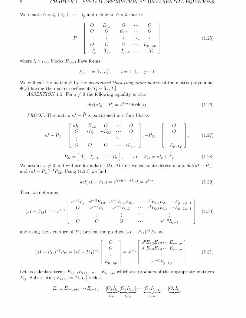
We denote n = l1 + l2 + · · ·+ lp and define an n× n matrix
P =
O E1,2 O · · · OO O E2,3 · · · O...
......
. . ....
O O O · · · Ep−1,p
−Tp −Tp−1 −Tp−2 · · · −T1
(1.25)
where li × li+1 blocks Ei,i+1 have forms
Ei,i+1 = [O, Ili], i = 1, 2, . . . p− 1
We will call the matrix P by the generalized block companion matrix of the matrix polynomialΦ(s) having the matrix coefficients Ti = [O, Ti].
ASSERTION 1.2. For s 6= 0 the following equality is true
det(sIn − P ) = sn−rpdetΦ(s) (1.26)
PROOF. The matrix sI − P is partitioned into four blocks
sI − P11 =
sIl1 −E1,2 O · · · OO sIl2 −E2,3 · · · O...
......
. . ....
O O O · · · sIlp−1
,−P12 =
OO...
−Ep−1,p
, (1.27)
−P21 =[
Tp Tp−1 · · · T2
]
, sI − P22 = sIr + T1 (1.28)
We assume s 6= 0 and will use formula (1.22). At first we calculate determinants det(sI − P11)and (sI − P11)
−1P12. Using (1.24) we find
det(sI − P11) = sl1+l2+···+lp−1 = sn−r (1.29)
Then we determine
(sI − P11)−1 = s1−p
sp−2Il1 sp−3E1,2 sp−4E1,2E2,3 · · · s0E1,2E2,3 · · ·Ep−2,p−1
O sp−2Il2 sp−3E1,2 · · · s1E2,3E3,4 · · ·Ep−2,p−1...
......
. . ....
O O O · · · sp−2Ilp−1
(1.30)
and using the structure of P12 present the product (sI − P11)−1P12 as
(sI − P11)−1P12 = (sI − P11)
−1
OO...
Ep−1,p
= s1−p
s0E1,2E2,3 · · ·Ep−1,p
s1E2,3E3,4 · · ·Ep−1,p...
sp−2Ep−1,p
(1.31)
Let us calculate terms Ei,i+1Ei+1,i+2 · · ·Ep−1,p, which are products of the appropriate matricesEij . Substituting Ei,i+1 = [O, Ili] yields
Ei,i+1Ei+1,i+2 · · ·Ep−1,p = [O, Ili]︸ ︷︷ ︸
li+1
[O, Ili+1]
︸ ︷︷ ︸
li+2
· · · [O, Ilp−1]
︸ ︷︷ ︸
lp=r
= [O, Ili]︸ ︷︷ ︸
r

1.2. BLOCK COMPANION CANONICAL FORMS OF TIME-INVARIANT SYSTEM 9
Then varying i from 1 to p− 1 we obtain
E1,2E2,3 · · ·Ep−1,p = [O, Il1]E2,3E3,4 · · ·Ep−1,p = [O, Il2]
...Ep−2,p−1Ep−1,p = [O, Ilp−2
]Ep−1,p = [O, Ilp−1
]
(1.32)
Substituting (1.32) in (1.31) gives the following expression
(sI − P11)−1P12 =
s1−p[O, Il1]s2−p[O, Il2]
...s−1[O, Ilp−1
]
(1.33)
Then inserting the right-hand sides of (1.29),(1.33) into (1.22) and using the blocks P21 andsI − P22 (1.28) we obtain
det(sIn − P ) = sn−rdet(sIr + T1 + [Tp, Tp−1, . . . , T2]
s1−p[O, Il1]s2−p[O, Il2]
...s−1[O, Ilp−1
]
) =
= sn−rdet(sIr+T1+[O, T2]s−1+[O, T3]s
−2, . . . , [O, Tp]s1−p) = sn−rdet((Irs
p+T1sp−1+· · ·+Tp)s1−p) =
= sn−r(sr(1−p)det(Irsp + T1s
p−1 + · · · + Tp)) = sn−rpdetΦ(s)
The assertion is proved.
Further we consider several canonical forms having the companion (block companion, gen-eral block companion) matrix of dynamics.
1.2.2 Controllable (observable) companion canonical form of single-input (output) systems
Let us consider controllable system (1.1),(1.2) with a scalar input u
x = Ax+ bu
y(t) = Cx (1.34)
where b is a nonzero constant column vector. We will find a linear nonsingular transformationof state variables
z = Nx (1.35)
with an nonsingular n× n matrix N that transforms (1.34) to the controllable canonical form[M4]
z = Az + bu
y = CN−1z (1.36)

10 CHAPTER 1. SYSTEM DESCRIPTION BY DIFFERENTIAL EQUATIONS
where A is the companion matrix of the characteristic polynomial φ(s) = sn + a1sn−1 + · · · +
an−1s+ an of the matrix A , i.e. A has the form (1.17), b is the n column vector
b =
0...01
(1.37)
The matrix CN−1 has no the special structure. For uniformity we will call (1.36) as thecontrollable companion canonical form.
Determination of transformation matrix N. Let us calculate the controllability matrixof the pair(A, b)
Y = [b, Ab, · · · , An−1b] =
0 0 0 · · · 10 0 0 · · · −a1...
......
. . ....
0 1 −a1 · · · · · ·1 −a1 −a2 + a2
1 · · · · · ·
(1.38)
Alternatively, substituting (1.35) into the first equation of (1.34) we obtain
z = NAN−1z +Nbu
Thus, A and b are expressed via A, N and b as follows
A = NAN−1, b = Nb
Writing the controllability matrix of the pair (NAN−1, Nb) as
Y = [Nb,NAb, · · · , NAn−1b] = NY (1.40)
where Y = [b, Ab, · · · , An−1b] is the n×n controllability matrix of the pair (A, b) we can expressN from (1.40) as
N = Y Y −1 (1.41)
Since the matrix Y is the lower triangular matrix then rankY = n and rankN = n. In theliterature it is usually used the matrix N−1 = Y Y −1 [A1], [M4] having the following simplestructure
Y −1 =
an−1 an−2 · · · a1 1an−2 an−3 · · · 1 0
......
.... . .
...a1 1 · · · 0 01 0 · · · 0 0
Thus, we show: if the pair (A, b) is controllable then the nonsingular transformation (1.35)with N from (1.41) always exists. This transformation reduces system (1.34) to the controllablecompanion canonical form (1.36). To calculate N it is enough to know the controllability matrixof the pair (A, b) and the characteristic polynomial of the dynamics matrix A.
Let us discover a structure of canonical system (1.36). Denoting variables of the vector zby zi, i = 1, 2, ..., n we can rewrite the first equation in (1.34) as follows
z1 = z2z2 = z3
...zn−1 = znzn = −anz1 − an−1z2 · · · − a1zn + u
(1.42)

1.2. BLOCK COMPANION CANONICAL FORMS OF TIME-INVARIANT SYSTEM 11
It is evident from (1.42) that the each state variable zi, i = 1, 2, ..., n − 1 is the integralof the following state variable zi+1 and zn is the integral of control u and signals aizj (i =n, n− 1, ..., 1; j = 1, 2, ..., n).
If l = 1, y = z1 then we can directly pass from the state space representation (1.42) to theinput-output representation (1.15) with r = 1, p = n, k = 1 and Fi = 1, i = 0, 1, . . . , n; B1 =1. Indeed, let us denote
y = z1, y = z2, y(2) = z3, · · · , y(n−1) = zn
Since y(n) = zn then substituting y(i) (i = 1, 2, ..., n) in the last equation of (1.42) gives a lineardifferential equation
y(n) + a1y(n−1) + · · · + any = u (1.43)
The dual result can be obtained for a observable system. If the system (1.34) has a scalar outputy, i.e. C is an n row vector, and the pair (A,C) is observable then (1.34) can be transformedinto the observable (companion) canonical form
z = Az + Bu
y = cz (1.44)
where A = AT , c = [0 0 · · · 0 1], matrix B has no special structure.
1.2.3 Controllable (observable) block companioncanonical form of multi-input(output) systems
Asseo’s form [A4]. Let us consider the controllable system (1.1),(1.2) with an r inputvector u ( r > 1 ). We will find a nonsingular transformation of state variables (1.35) whichreduces the system to the canonical form having the block companion matrix of dynamics (see1.20). This canonical form have been first obtained by Asseo [A4] in 1968.
Let us propose that rankB = r. We define the controllability index of the pair (A,B) asthe smallest integer ν(ν ≤ n) such that
rank[
B, AB, · · · , An−1B]
= rank[
B, AB, · · · , Aν−1B]
(1.45)
and consider a system with n = rν , i.e. r is the divisor of n. Only such type a system is reducedto the canonical form with the block companion matrix of dynamics (1.20). This canonical form(Asseo’s form) is the particular case of Yokoyama’s canonical form where rν > n.
Let the transformation z = Nz reduces system (1.1), (1.2) to a canonical form
z = A∗z +B∗u
y = C∗z (1.46)
where A∗ = NAN−1 is block companion matrix (1.20): A∗ = P ∗ with p = ν and
B∗ = NB =
[
OIr
]
(1.47)
The matrix C∗ = CN−1 has no special structure. We will call (1.46) as the controllable block
companion canonical form a the multi-input system.

12 CHAPTER 1. SYSTEM DESCRIPTION BY DIFFERENTIAL EQUATIONS
Determination of transformation matrix N. The matrix N is partitioned as
N =
Nν
Nν−1...N1
(1.48)
where Ni are r × n submatrices. Since A∗ = NAN−1 then substituting (1.20) for P ∗ = A∗,p = ν and (1.48) for N into the equality A∗N = NA gives the following matrix equation
O Ir O · · · OO O Ir · · · O...
......
. . ....
O O O · · · Ir−Tp −Tp−1 −Tp−2 · · · −T1
Nν
Nν−1...N2
N1
=
Nν
Nν−1...N2
N1
A
from which blocks Ni (i = 1, 2, . . . , ν) are defined as follows
Nν−1 = NνANν−2 = Nν−1A = NνA
2
...N1 = N2A = NνA
ν−1
(1.49)
Thus, any block Ni (i = 1, 2, . . . , ν) is defined via the block Nν . To determine Nν we shall usethe approach of Sec.1.2.2. Since A∗ = NAN−1, B∗ = NB then we can express blocks of thecontrollability matrix of the pair (A∗, B∗) via matrices A,B,C as follows
Y ∗ = [B∗, A∗B∗, . . . , (A∗)n−1B∗] = [NB,NAB, . . . , NAn−1B] = N [B,AB, . . . , An−1B]
From this equality we obtain
(A∗)i−1B∗ = NAi−1B, i = 1, 2, . . . , n (1.50)
Blocks AkB (k > ν − 1) are linearly dependent on AkB (k ≤ ν − 1) because the pair (A,B)has the controllability index ν and satisfies the condition (1.45).
Let us consider the n× n matrix Y ∗ = [B∗, A∗B∗, . . . , (A∗)ν−1B∗]. Using (1.50) we have
Y ∗ = N [B,AB, . . . , Aν−1B] (1.51)
Calculating products (A∗)iB∗ with A∗ and B∗ from (1.20) and (1.47) we reveal the structureof the matrix Y ∗
Y ∗ =[
B∗, A∗B∗, . . . , (A∗)ν−1B∗
]
=
O O · · · O IrO O · · · Ir −T1...
.... . .
......
0 Ir · · · X XIr −T1 · · · X X
(1.52)
where X are some unspecified submatrices. The matrix Y ∗ is nonsingular one because it hasunity blocks on the diagonal, i.e. rankY ∗ = n. Substituting the right-hand side of (1.52) into

1.2. BLOCK COMPANION CANONICAL FORMS OF TIME-INVARIANT SYSTEM 13
the left-hand side of (1.51) we obtain the equality
O O · · · O IrO O · · · Ir −T1...
.... . .
......
0 Ir · · · X XIr −T1 · · · X X
=
Nν
Nν−1...N2
N1
[
B, AB, · · · , Aν−1B]
(1.53)
from which it follows the equation for Nν
Nν
[
B, AB, · · · , Aν−1B]
=[
O, O, · · · , O, Ir]
(1.54)
ThusNν =
[
O, O, · · · , O, Ir] [
B, AB, · · · , Aν−1B]−1
(1.55)
Others blocks Ni, i = 1, 2, . . . , ν − 1 are calculated by formulas (1.49). It should be noted thatobtained blocks Ni,i = 1, 2, . . . , ν − 1 satisfy relation (1.53). Indeed, the following equalitiestake place from (1.49) and (1.54)
Nν−1
[
B, AB, · · · , Aν−1B]
= NνA[
B, AB, · · · , Aν−1B]
=
= Nν
[
AB, A2B, · · · , AνB]
=[
O, O, · · · , O, Ir, X]
,
Nν−2
[
B, AB, · · · , Aν−1B]
= = NνA2[
B, AB, · · · , Aν−1B]
=
= Nν
[
A2B, A3B, · · · , Aν+1B]
=[
O, O, · · · , O, Ir, X, X]
and so on.The matrix N is nonsingular one. It follows from nonsingularity of the matrix in the left-
hand side of (1.53) and the matrix [B,AB, · · · , Aν−1B].Thus, we show: if the pair matrix (A,B) is controllable with the controllability index
ν = n/r and rankB = r then the nonsingular transformation z = Nx with N from (1.48),(1.49), (1.54) always exists. This transformation reduces system (1.1),(1.2) to the canonicalform (1.46).
The analogous dual result can be obtained for an observable system. Let rankC = l andthe pair (C,A) is observable with the observability index α, which is a smallest integer such as
rank[CT , AT , CT , ..., (AT )n−1CT ] = rank[CT , AT , CT , ..., (AT )α−1CT ] = n
Let α = n/l. Then system (1.1), (1.2) can be transformed into the observable block companioncanonical form
z = Az + Bu
y = Cz
where A = (P ∗)T ,C = [O,O, . . . , O, Il] and matrix B has no special structure.Let us consider the structure of the canonical system (1.46). We introduce subvectors zi,
i = 1, 2, . . . , ν
z1 =
z1z2...zr
, z2 =
zr+1
zr+2...z2r
, · · ·

14 CHAPTER 1. SYSTEM DESCRIPTION BY DIFFERENTIAL EQUATIONS
where zi, i = 1, 2, . . . , n are components of the vector z. Using these notions and the blockstructure of A∗ we rewrite the first equation in (1.46) as follows
˙z1 = z2˙z2 = z3
...˙zν−1 = zν˙zν = −Tν z1 − Tν−1z2 · · · − T1zν + Iru
(1.56)
In (1.56) the each group of state variables zi (i = 1, 2, . . . , ν − 1) is the integral of the nextgroup zi+1 and zν is the integral of the control vector u and vectors Tizj (i = ν, ν − 1, . . . , 1;j = 1, 2, . . . , ν). The general structure of (1.56) coincides with the structure of (1.42) withn = ν, zi = zi, ai = Ti, CN
−1 = [C1, C2, . . . , Cν ] where Ci are l × r submatrices.Let us show that for l = r we can pass from the state-space representation (1.56) to the
input-output representation (1.15). In fact, defining the output vector for (1.56) as y = z1 andusing (1.56) we obtain
y = z1, ˙y = z2, · · · , y(ν−1) = zν
So far as
y(ν) = z(1)ν = −Tν z1 − Tν−1z2 − · · · − T1zν + Iru
then replacing zi by y(i) in the last expression we obtain
y(ν) = −Tν y − Tν−1y(1) − Tν−2y
(2) − · · · − T1y(ν−1) + Iru (1.57)
The vector differential equation (1.57) coincides with (1.15) when p = ν, Fp = Ir, Bo = Ir,Bi = O (i = 1, 2, . . . , k).
Yokoyama’s form [Y1], [Y2]. Let us consider the general case of system (1.1), (1.2) withr input vector u (r > 1), rankB = r and the controllability index ν 6= n/r, i.e. r does not thedivisor of n: n < rν . Using the nonsingular transformation of state variables (1.35) and inputvariables
v = M−1u (1.58)
where M is an r × r permutation2 matrix we can reduce system (1.1), (1,2) to the canonicalform with the general block companion matrix of dynamics (1.25). This canonical form havebeen worked out by Yokoyama in 1972 [Y1].
For a pair of matrices A and B with the controllability index ν we define the integersl1, l2, . . . , lν by the rule
l1 = rank[B,AB, · · · , Aν−1B] − rank[B,AB, · · · , Aν−2B]
l2 = rank[B,AB, · · · , Aν−2B] − rank[B,AB, · · · , Aν−3B]
· · · (1.59)
lν−1 = rank[B,AB] − rankB
lν = rankB = r
From (1.59) it follows that
l1 ≤ l2 ≤ · · · ≤ lν (1.60)
2A permutation matrix has a single unity element in each row (column) and zeros otherwise.

1.2. BLOCK COMPANION CANONICAL FORMS OF TIME-INVARIANT SYSTEM 15
Let us determine the sum of li ,i = 1, 2, . . . , ν by adding the left-hand and the right-hand sidesof (1.59). We obtain the relation
l1 + l2 + · · · lν = rank[B,AB, . . . , Aν−1B] = n
Now we use transformation (1.35), (1.58) to reduce system (1.1), (1.2) to Yokoyama’s canon-ical form
z = Fz +Gv
y = CN−1z (1.61)
where the matrix F = NAN−1 is the general block companion matrix of the structure (1.25)with p = ν, n = n, −Tp = Fν1, −Tp−1 = Fν2, . . ., −T1 = Fνν
F =
O E1,2 O · · · OO O E2,3 · · · O...
......
. . ....
O O O · · · Eν−1,ν
Fν1 Fν2 Fν3 · · · Fνν
(1.62)
and blocks Ei,i+1 of the form
Ei,i+1 = [O, Ili], i = 1, 2, . . . , ν − 1 (1.63)
In (1.62) blocks Fνi have the increasing numeration for convenience. In (1.61) the matrixG = NBM has the form
G =
[
OGν
]
(1.64)
where an r × r block Gν is a lower triangular matrix with unity diagonal elements
Gν =
I1 O · · · OX I2 · · · O...
.... . .
...X X · · · Iν
(1.65)
Here I i, i = 1, 2, . . . , ν are unity matrices of orders lν−i+1 − lν−i, lo = 0, X are some unspecifiedsubmatrices. Let us note that the matrix CN−1 has no special structure. We will call (1.61)as the controllable generalized block companion canonical form or Yokoyama’s form.
Determination of transformation matrix N [S3]. At first we construct the n × rνmatrix containing the first ν blocks AiB, i = 0, 1, . . . , ν − 1 of the controllability matrixB,AB, . . . , An−1B satisfying the equality
rank[B,AB, . . . , Aν−1B] = n
Let us find a permutation matrix M rearranging columns of B such that the matrix
[BM,ABM, . . . , Aν−1BM ]
has linearly independent columns in last columns of AiBM ,i = 0, 1, . . . , ν − 1. From (1.59) itfollows that the blocks AiBM maintain lν−i linearly independent columns.
16 CHAPTER 1. SYSTEM DESCRIPTION BY DIFFERENTIAL EQUATIONS
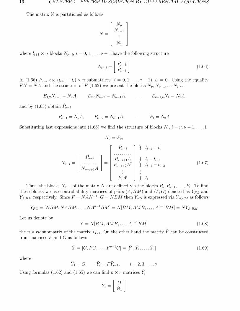
The matrix N is partitioned as follows
N =
Nν
Nν−1...N1
where li+1 × n blocks Nν−i, i = 0, 1, . . . , ν − 1 have the following structure
Nν−i =
[
Pν−iPν−i
]
(1.66)
In (1.66) Pν−i are (li+1 − li) × n submatrices (i = 0, 1, . . . , ν − 1), lo = 0. Using the equalityFN = NA and the structure of F (1.62) we present the blocks Nν , Nν−1, . . .N1 as
E1,2Nν−1 = NνA, E2,3Nν−2 = Nν−1A, . . . Eν−1,νN1 = N2A
and by (1.63) obtain Pν−i
Pν−1 = NνA, Pν−2 = Nν−1A, . . . P1 = N2A
Substituting last expressions into (1.66) we find the structure of blocks Ni, i = ν, ν − 1, . . . , 1
Nν = Pν ,
Nν−i =
Pν−i. . . . . . . .Nν−i+1A
=
Pν−i. . . . . . . . .Pν−i+1APν−i+2A
2
...PνA
i
li+1 − li
li − li−1
li−1 − li−2... l1
(1.67)
Thus, the blocks Nν−1 of the matrix N are defined via the blocks Pν , Pν−1, . . . , P1. To findthese blocks we use controllability matrices of pairs (A,BM) and (F,G) denoted as YFG andYA,BM respectively. Since F = NAN−1, G = NBM then YFG is expressed via YA,BM as follows
YFG = [NBM,NABM, . . . , NAn−1BM ] = N [BM,AMB, . . . , An−1BM ] = NYA,BM
Let us denote byY = N [BM,AMB, . . . , Aν−1BM ] (1.68)
the n× rν submatrix of the matrix YFG. On the other hand the matrix Y can be constructedfrom matrices F and G as follows
Y = [G,FG, . . . , F ν−1G] = [Y1, Y2, . . . , Yν] (1.69)
whereY1 = G, Yi = F Yi−1, i = 2, 3, . . . , ν
Using formulas (1.62) and (1.65) we can find n× r matrices Yi
Y1 =
[
OΘ1
]

1.2. BLOCK COMPANION CANONICAL FORMS OF TIME-INVARIANT SYSTEM 17
Yi =
O O. . . .X Θi
. . . .X X
l1 + l2 + · · · + lν−i
lν−i+1 (1.70)
where square matrices Θi of the order lν−i+1 are lower triangular matrices
Θ1 = Gν , Θi =
I i O · · · OX I i+1 · · · O...
.... . .
...X X · · · Iν
, i = 2, 3, . . . , ν (1.71)
In (1.71) I i are unity matrices of the order lν−i+1 − lν−i, lo = 0, X are some matrices. From(1.68) and (1.69) we obtain the relation
Nν
Nν−1...N1
[BM,AMB, . . . , Aν−1BM ] = [Y1, Y2, . . . , Yν ] (1.72)
Let us denote lν−i+1 last (linearly independent) block columns of the submatrix Aν−1BM byVi, i = 2, . . . , ν
Vi = Ai−1BM
[
OIlν−i+1
]
, i = 2, . . . , ν, V1 = BM (1.73)
The matrix V = [V1, V2, . . . , Vν ] of the size n×∑νi=1 li = n×n is the nonsingular square matrix.
Using (1.72),(1.70) we find structure of the product NV
Nν
Nν−1...N1
[V1, V2, . . . , Vν] =
O O · · · O O Θν
O O · · · O Θν−1 XO O · · · Θν−2 X X...
... · · · ......
...O Θ2 · · · X X XΘ1︸︷︷︸
lν
X︸︷︷︸
lν−1
· · · X X︸︷︷︸
l2
X︸︷︷︸
l1
l1 l2 l3.........
(1.74)
where X are some unspecified submatrices. Taking into account that Pi are (lν−i+1 − lν−i)× nupper blocks of Ni and matrices Θi have the structure (1.71) as well as using the equalityNV1 = G we can rewrite relation (1.74) in terms of blocks Pi, i = 1, 2, . . . , ν
PνPν−1
...P1
[V1, V2, . . . , Vν ] =
O O... · · · ... O O
... O O... Iν
O O... · · · ... O O
... Iν−1 O... X
O O... · · · ... Iν−2 O
... X X... X
......
... · · · ......
......
......
......
I1 O... · · · ... X X
... X X... X
l1 l2 − l1 l3 − l2... lν − lν−1
(1.75)where matrix block columns have sizes n × lν , n × lν−1, . . . , n × l1 respectively, blocks X aresome unspecified submatrices. Equation (1.75) may be used for calculating blocks Pi. Thenmatrices Ni are obtained by relation (1.67).

18 CHAPTER 1. SYSTEM DESCRIPTION BY DIFFERENTIAL EQUATIONS
Let us demonstrate that these Ni satisfy (1.74). At first we evaluate the block NνV
NνV = PνV = Pν [V1, V2, . . . , Vν] = [O,O, . . . , O, Iν] (1.76)
Then we find the block Nν−1V
Nν−1V =
[
Pν−1VPνAV
]
=
[
Pν−1[V1, V2, . . . , Vν]Pν [AV1, AV2, . . . , AVν ]
]
Using (1.75) we obtain
Pν−1[V1, V2, . . . , Vν] = [O,O, . . . , Iν−1, O,X] (1.77)
and find blocks PνAVi, i = ν, ν − 1, . . . , 1 of the matrix PνAV = Pν [AV1, AV2, . . . , AVν ]. From
(1.73) it follows Vν = AVν−1
[
OIl1
]
. Thus
PνAVν−1 = Pν(AVν−1
[
Il2−l1O
]
, AVν−1
[
OIl1
]
) = Pν(AVν−1
[
Il2−l1O
]
, Vν) = [X, Iν ]
Other products PνAVi , i = 1, 2, . . . , ν − 2 are equaled to zeros because columns of matricesAV1,. . . , AVν−1 are linearly dependent on blocks V1, V2, . . . , Vν−1 for which equality (1.76) istrue. We result in
PνAV = [O,O, . . . , O,X, Iν, X]
Uniting (1.77) with the last expression we find
Nν−1V =
[
O O · · · Iν−1 O XO O · · · X Iν X
]
=[
O, O, · · · , Θν−1, X]]
Now it is evident that the right-hand side of the last formula coincides with the second blockrow of the matrix in the right-hand side of (1.74). And so on.
Then we need to show that the matrix G = NBM coincides with (1.64). CalculatingNνBM,Nν−1BM, . . . , N1BM and using BM = V1 we obtain from (1.74) that
NiBM = O, i = 1, ν, . . . , 2, N1BM = Θ1 = Gν
REMARK 1.2. For l1 = l2 = · · · = lν = r (Asseo’s form) we have ν = n/r, V1 = B, V2 =AB, . . . , Vν = Aν−1B, li = r, li+1 − li = 0 (i = 1, 2, . . . , ν − 1), M = Ir, Nν = Pν .Therefore, equation (1.75) may be rewritten as
Pν[
B, AB, · · · , Aν−1B]
=[
O, O, · · · , O, Ir]
The matrix N has the following simple structure
N =
Nν
Nν−1...N1
=
PνPνA
...PνA
ν−1
Let us note that the last formula coincides with (1.54), (1.49) respectively. So, Asseo’s form isthe particular case of Yokoyama’s form.

1.2. BLOCK COMPANION CANONICAL FORMS OF TIME-INVARIANT SYSTEM 19
REMARK 1.3. If rankC = l and the pair (A,C) is observable with the observability indexα < n/l then system (1.1), (1.2) can be transformed into the observable generalized blockcompanion canonical form
z = Az + Bu
y = Cz
where A and C areA = F T , C = [O,O, . . . , O, GT
α]
Let us show that the structure of canonical system (1.61) resembles with (1.42) or (1.56).We combine components zi, i = 1, . . . , n of the vector z into subvectors z1, z2, . . . , zν by the rule
z1 =
z1z2...zl1
, z2 =
zl1+1
zl1+2...
zl1+l2
, · · ·
Using the block structure of F we can rewrite the first equation in (1.61) as
˙z1 = [O, Il1]z2˙z2 = [O, Il2]z3
...˙zν−1 = [O, Ilν−1
]zν˙zν = Fν1z1 + Fν2z2 + · · · + Fνν zν +Gνv
(1.78)
In (1.78) the each subvector zi is the integral of last components of the subvector zi+1 and zνis the integral of the control vector Gνv and vectors Fνizi, i = 1, 2, . . . , ν.
Now let us show that for l = r it is possible to transfer from the state-space representation(1.78) to the input-output representation (1.15), which is set of linear differential equations ofthe order ν. For this purpose we introduce the r vector y containing li − li−1 subvectors yi(i = 1, . . . , ν), lo = 0
y =
yνyν−1
...y1
(1.79)
Denoting
z1 = y1, z2 =
[
y2
y1
]
, z3 =
y(2)3
y(2)2
y(2)1
, · · · , zν =
y(ν−1)ν
y(ν−1)ν−1...
y(ν−1)1
and using (1.79) we express
z1 = [O, Il1]y, z2 = [O, Il2]y, · · · , zν−1 = [O, Ilν−1]y(ν−2), zν = y(ν−1) (1.80)
Sincey(ν) = ˙zν = Fν1z1 + Fν2z2 + · · ·+ Fνν zν +Gνv
then replacing zi by y(i) in the last equation
y(ν) = Fν1[O, Il1]y + Fν2[O, Il2]y + · · ·+ Fννy(ν−1) +Gνv

20 CHAPTER 1. SYSTEM DESCRIPTION BY DIFFERENTIAL EQUATIONS
and performing multiplications we get
y(ν) = [O,Fν1]y + [O,Fν2]y + · · ·+ [O,Fνν]y(ν−1) +Gνv (1.81)
This vector differential equation coincides with (1.15) when p = ν, Fp = Ir, Fi = −[O,Fνi] (i =1, . . . , ν − 1), Bi = O(i 6= 0), Bo = Gν .
Let us consider several examples.EXAMPLE 1.1.
We need to find the controllable canonical form of the system with n = 3 and r = 1
x =
2 1 00 1 11 0 0
x+
100
u (1.82)
Since detY = det[b, Ab, A2b] = −1 6= 0 then the system is controllable. We calculate a charac-teristic polynomial of A: φ(s) = det(sI − A) = s3 + a1s
2 + a2s + a3 = s3 − 3s2 + 2s − 1and find a3 = −1, a2 = 2, a1 = −3. Now we construct matrices Y = [b, Ab, A2b] and
Y −1 =
a2 a1 1a1 1 01 0 0
and calculate
Y =
1 2 40 0 10 1 2
, Y −1 =
2 −3 1−3 1 0
1 0 0
By formula (1.41) we find
N−1 =
0 −1 11 0 0
−1 1 0
Since
N =
0 1 00 1 11 1 1
then using formula (1.39) we obtain
A = NAN−1 =
0 1 00 0 11 −2 3
, b =
001
(1.83)
It is evident that the matrix A in (1.83) is the companion matrix of the polynomial φ(s) =s3 − 3s2 + 2s− 1.
EXAMPLE 1.2.
Let us consider the following system with n = 4, r = 2
x =
2 1 0 11 0 1 11 1 0 00 0 1 0
x+
1 00 00 00 1
u (1.84)
Since det[B,AB] = det
1 0 2 10 0 1 10 0 1 00 1 0 0
= −1 then the system is controllable with the con-
trollability index ν = 2 = n/r and can be transformed into the controllable block companion

1.2. BLOCK COMPANION CANONICAL FORMS OF TIME-INVARIANT SYSTEM 21
canonical form (Asseo’s form). Let us find the related transformation matrix N . It has thefollowing structure
N =
[
N2
N1
]
=
[
N2
N2A
]
(1.85)
where the 2 × 4 submatrix N2 is calculated from equation (1.54)
N2[B,AB] = [O, I2]
Since
[B,AB]−1 =
1 −1 −1 00 0 0 10 0 1 00 1 −1 0
then we can find
N2 = [O, I2][B,AB]−1 =
[
0 0 1 00 1 −1 0
]
and using (1.85) calculate
N =
0 0 1 00 1 −1 01 1 0 00 −1 1 1
(1.86)
As
N−1 =
−1 −1 1 01 1 0 01 0 0 00 1 0 1
(1.87)
then we find
A∗ = NAN−1 =
0 0 1 00 0 0 1
−1 0 3 21 0 0 −1
, B∗ = NB =
0 00 01 00 1
(1.88)
Matrix A∗ in (1.88) is the block companion matrix for the matrix polynomial Φ(s) = I2s2 +
T1s+ T2 with
T1 =
[
−3 −21 0
]
, T2 =
[
1 0−1 0
]
.
EXAMPLE 1.3.
Let us find Yokoyama’s canonical form for the controllable system with n = 4, r = 2 [S3]
x =
2 1 0 00 1 0 10 2 0 01 1 0 0
x+
1 00 00 00 1
u (1.89)
At first we build the controllability matrix YAB = [B,AB,A2B,A3B]. As rank[B,AB,A2B] =4 then ν = 3. Using formulas (1.59) we calculate l1 = l2 = 1, l3 = 2. Since
rank[B,AB,A2B] = rank[b1, b2, Ab2, A2b2]

22 CHAPTER 1. SYSTEM DESCRIPTION BY DIFFERENTIAL EQUATIONS
where b1, b2 are columns of the matrix B then M is the unity matrix
M =
[
1 00 1
]
(1.90)
Let us find the matrix V = [V1, V2, V3]. Using (1.73) we find
V1 = [b1, b2] =
1 00 00 00 1
, V2 = AV1
[
01
]
=
0100
, V3 = AV2 =
1121
and by formulas (1.67) discover the structure of the matrix N
N =
N3
. .N2
. .N1
=
P3
. . . . .P3A. . . . .P1
P3A2
(1.91)
where N3 = P3 is an 1 × 4 submatrix (l1 = 1). Here a submatrix P2 does’t exist becausel2 − l1 = 0 and N2 = P3A. Submatrices P1 and P3 are satisfied the following equation
[
P3
P1
]
[V1, V2, V3] =
0 0
... 0... 1
1 0... x1
... x2
l1 = 1 l3 − l2 = 1
(1.92)
that follows from formula (1.75) for the concrete l1 = 1, l2 = 1, l3 = 2. In (1.92) x1 and x2 areany numbers. Assigning x1 = 0, x2 = 1 we calculate from (1.92)
P3 = [0 0 0.5 0]
P1 = [1 0 0 0]
and find N from (1.91)
N =
0 0 0.5 00 1 0 01 0 0 00 1 0 1
(1.93)
Thus
F = NAN−1 =
0 1 0 00 0 0 10 1 2 00 1 1 1
, G = NB =
0 00 01 00 1
(1.94)
It is evident that the structure of matrices F and G corresponds formulas (1.62)-(1.65). Indeed,in (1.62)
E1,2 = 1, E2,3 = [0 1], F31 =
[
00
]
, F32 =
[
11
]
, F33 =
[
2 01 1
]
and in (1.64), (1.65) I1 = 1, I2 does not exist, I3 = 1 . The matrix F in (1.94) is the generalblock companion matrix for the matrix polynomial
Φ(s) = I2s3 + T1s
2 + T2s+ T3

1.2. BLOCK COMPANION CANONICAL FORMS OF TIME-INVARIANT SYSTEM 23
with
T1 = −F33 =
[
−2 0−1 −1
]
, T2 = −[O, F32] =
[
0 −10 −1
]
, T3 = −[O, F31] =
[
0 00 0
]
For testing we find detΦ(s) = det
[
s3 − 2s2 −s−s2 s3 − s2 − s
]
= s3(s3 − 3s2 + s+1) and
det(sI4−F ) = s4−3s3 +s2 +s. It is evident that s−2detΦ(s) = det(sI4−F ). The last equalitycorresponds to Assertion 1.2 (formula (1.26)).

24 CHAPTER 1. SYSTEM DESCRIPTION BY DIFFERENTIAL EQUATIONS

Chapter 2
System description by transfer functionmatrix
2.1 The Laplace transform
Let’s consider a scalar function f(t) of a real variable t such that the function f(t)e−st wheres is a complex variable has a convergent integral
f(s) =∫
∞
0f(t)e−stdt (2.1)
This integral is known as a direct one-sided Laplace transform of a time-dependent function ora Laplace integral. It is calculate, by definition, as follows
∫∞
0f(t)e−stdt = lim
T→∞,ǫ→0
∫ T
ǫf(t)e−stdt
If a limit exists then the Laplace integral is a convergent integral. These questions arestudied detail in any textbooks, for example in [B3].
A function f(s) of a complex variable s is called the Laplace transform of f(t) and denotedas L[f(t)] = f(s). Let us write the main properties of the Laplace transform which will beuseful in the present study. Let f(t), fi(t), i = 1, 2 are scalar functions of time and a, b areconstant variables. We have
1.L[af1(t) + bf2(t)] = af1(s) + bf2(s)
where L[f1(t)] = f1(s) , L[f2(t)] = f2(s)2.
L[f (i)(t)] = sif(s) − f(+0)si−1 − · · · − f (i−1)(+0), f(+0) = limt→+0
f(t)
3.L[∫
f(t)dt] = f(s)/s+ (∫
f(t)dt/t=+0)/s
4.L[f(t− a)] = e−asf(s), for a > 0
5.L[~f(t)] = ~f(s) (2.2)
25
26 CHAPTER 2. SYSTEM DESCRIPTION BY TRANSFER FUNCTION MATRIX
where ~f(t), ~f(s) are n-vectors.Thus, the Laplace transform makes possible to replace a differential equation in f(t) by
an algebraic equation in f(s). Solving the algebraic equation we can find f(s). For obtainingf(t) we should use the inverse Laplace transform ( L−1 - transform). For more details see, forexample, [B3].
2.2 Transformation from state-space to
frequency domain representation.
Transfer function matrix
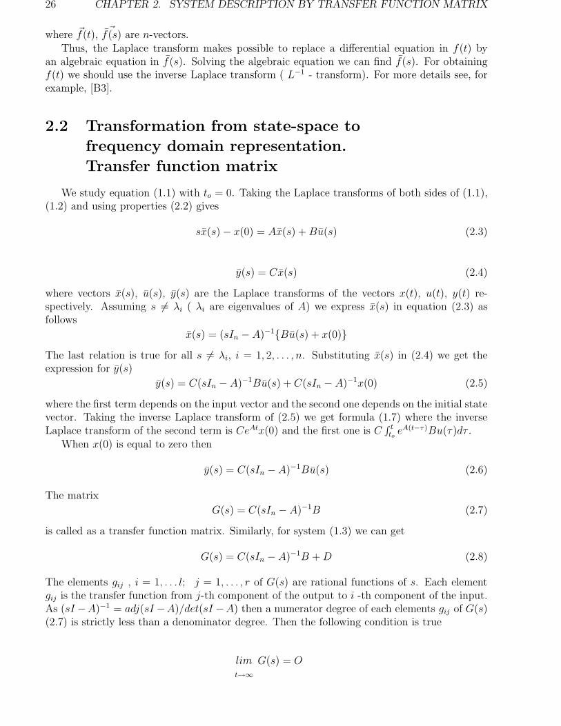
We study equation (1.1) with to = 0. Taking the Laplace transforms of both sides of (1.1),(1.2) and using properties (2.2) gives
sx(s) − x(0) = Ax(s) +Bu(s) (2.3)
y(s) = Cx(s) (2.4)
where vectors x(s), u(s), y(s) are the Laplace transforms of the vectors x(t), u(t), y(t) re-spectively. Assuming s 6= λi ( λi are eigenvalues of A) we express x(s) in equation (2.3) asfollows
x(s) = (sIn − A)−1Bu(s) + x(0)The last relation is true for all s 6= λi, i = 1, 2, . . . , n. Substituting x(s) in (2.4) we get theexpression for y(s)
y(s) = C(sIn −A)−1Bu(s) + C(sIn − A)−1x(0) (2.5)
where the first term depends on the input vector and the second one depends on the initial statevector. Taking the inverse Laplace transform of (2.5) we get formula (1.7) where the inverseLaplace transform of the second term is CeAtx(0) and the first one is C
∫ tto e
A(t−τ)Bu(τ)dτ .When x(0) is equal to zero then
y(s) = C(sIn −A)−1Bu(s) (2.6)
The matrix
G(s) = C(sIn − A)−1B (2.7)
is called as a transfer function matrix. Similarly, for system (1.3) we can get
G(s) = C(sIn − A)−1B +D (2.8)
The elements gij , i = 1, . . . l; j = 1, . . . , r of G(s) are rational functions of s. Each elementgij is the transfer function from j-th component of the output to i -th component of the input.As (sI −A)−1 = adj(sI −A)/det(sI −A) then a numerator degree of each elements gij of G(s)(2.7) is strictly less than a denominator degree. Then the following condition is true
limt→∞
G(s) = O
2.3. PHYSICAL INTERPRETATION OF TRANSFER FUNCTION MATRIX 27
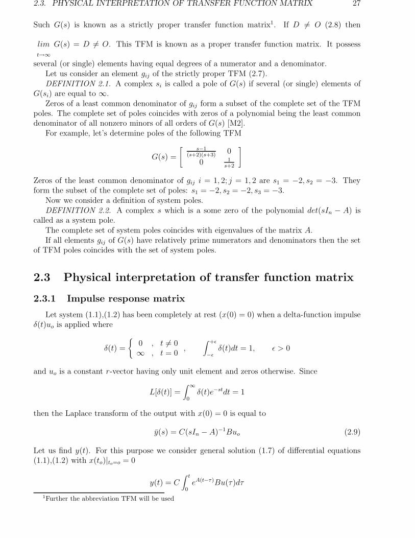
Such G(s) is known as a strictly proper transfer function matrix1. If D 6= O (2.8) then
limt→∞
G(s) = D 6= O. This TFM is known as a proper transfer function matrix. It possess
several (or single) elements having equal degrees of a numerator and a denominator.Let us consider an element gij of the strictly proper TFM (2.7).DEFINITION 2.1. A complex si is called a pole of G(s) if several (or single) elements of
G(si) are equal to ∞.Zeros of a least common denominator of gij form a subset of the complete set of the TFM
poles. The complete set of poles coincides with zeros of a polynomial being the least commondenominator of all nonzero minors of all orders of G(s) [M2].
For example, let’s determine poles of the following TFM
G(s) =
[s−1
(s+2)(s+3)0
0 1s+2
]
Zeros of the least common denominator of gij i = 1, 2; j = 1, 2 are s1 = −2, s2 = −3. Theyform the subset of the complete set of poles: s1 = −2, s2 = −2, s3 = −3.
Now we consider a definition of system poles.DEFINITION 2.2. A complex s which is a some zero of the polynomial det(sIn − A) is
called as a system pole.The complete set of system poles coincides with eigenvalues of the matrix A.If all elements gij of G(s) have relatively prime numerators and denominators then the set
of TFM poles coincides with the set of system poles.
2.3 Physical interpretation of transfer function matrix
2.3.1 Impulse response matrix
Let system (1.1),(1.2) has been completely at rest (x(0) = 0) when a delta-function impulseδ(t)uo is applied where
δ(t) =
0 , t 6= 0∞ , t = 0
,∫ +ǫ
−ǫδ(t)dt = 1, ǫ > 0
and uo is a constant r-vector having only unit element and zeros otherwise. Since
L[δ(t)] =∫
∞
0δ(t)e−stdt = 1
then the Laplace transform of the output with x(0) = 0 is equal to
y(s) = C(sIn −A)−1Buo (2.9)
Let us find y(t). For this purpose we consider general solution (1.7) of differential equations(1.1),(1.2) with x(to)|to=o = 0
y(t) = C∫ t
0eA(t−τ)Bu(τ)dτ
1Further the abbreviation TFM will be used

28 CHAPTER 2. SYSTEM DESCRIPTION BY TRANSFER FUNCTION MATRIX
Setting u(τ) = δ(τ)uo in the last equation we obtain
y(t) = C∫ t0 e
A(t−τ)Bδ(τ)uodτ = C(∫ to e
A(t−τ)δ(τ)dτ)Buo =
C∫ t0 e
Atδ(t− τ)dτBuo = CeAtBuo
The matrixG(t) = CeAtB (2.10)
is called as the impulse response matrix of a system [W1].Using the Laplace transform of eAt: L[eAt] = (sIn − A)−1 we find
L[G(t)] = C(sIn − A)−1B = G(s)
So, TFM G(s) is the Laplace transform of a impulse response matrix.
2.3.2 Frequency response matrix
It is known that exponential functions est with a complex parameter s describe oscillatorysignals of all frequencies with a constant or exponential amplitude. Indeed, if s = jω is animaginary variable then ejωt = cosωt + jsinωt and cosωt = 0.5(ejωt + e−jωt). So, we have anoscillatory function with the frequency ω . If s is a complex variable: s = s + jω ( s - realvariable ) then est = est(cosωt+jsinω). Thus we have an oscillatory signal with the exponentialincreasing or decreasing amplitude and the frequency ω. Applying an exponential input signalwe can reveal a relationship between TFM and the transient response of a system.
Suppose we use an exponential input having the following form
u(t) =
0 , t ≤ 0uoe
st , t > 0(2.11)
The function (2.11) can be rewritten as follows
u(t) = uoest1(t) (2.12)
where s is a complex variable, uo is a constant r vector, 1(t) denotes a unit step function oftime
1(t) =
0 , t ≤ 01 , t > 0
Let us write a general solution of (1.1), (1.2) with the input (2.12). Assuming that s does notcoincide with any eigenvalue of A we obtain
y(t) = CeAtx(0) + C∫ t
0eA(t−τ)Buoe
stdτ = CeAtx(0) + CeAt∫ t
0e−AτBuoe
sτdτ
We consider the second item. Since
Buoesτ = BuoIne
sτ = InesτBuo = eInsτBuo
then we can write
y(t) = CeAtx(0) + CeAt∫ t
0e(sIn−A)τBuodτ (2.13)
The vector Buo does not depend in τ , therefore, it should be taken out from the integral
y(t) = CeAtx(0) + CeAt∫ t
0e(sIn−A)τdτBuo

2.4. PROPERTIES OF TRANSFER FUNCTION MATRIX 29
Integrating we have
∫ t
0e(sIn−A)τdτ = e(sIn−A)τ |t0(sIn − A)−1 = (e(sIn−A)t − In)(sIn − A)−1
Substituting the right-hand side of the last relation in (2.13) we obtain
y(t) = CeAtx(0) + CeAt(e(sIn−A)t − In)(sIn − A)−1Buo =
CeAtx(0) + Cest(sIn −A)−1Buo − CeAt(sIn − A)−1Buo =
CeAtx(0) − (sIn − A)−1Buo + C(sIn −A)−1Buoest
In this expression the second term is equal to G(s)u(t). The first term is determined duesystem response in the initial time. If the system is asymptotically stable ( Reλi(A) < 0 ) andRes > Reλi, i = 1, . . . , n then we have for large values of t
y(t) ∼= G(s)u(t), t≫ 0 (2.14)
Thus, the transfer function matrix G(s) describes asymptotic behavior of a system in responseto exponential inputs of the complex frequency s.
Let us consider the oscillatory input
u(t) = uoejωt1(t), t ≥ 0 (2.15)
where a real value ω is the frequency of the oscillation. Substituting (2.15) in (2.14) yields
y(t) ∼= G(jω)u(t)
where G(jω) = C(jωIn − A)−1B is called as the frequency response matrix.So, it has been shown that TFM with s = jω coincides with the frequency response matrix.
2.4 Properties of transfer function matrix
2.4.1 Transformation of state, input and output vectors
Let’s carry out a nonsingular transformation of the state vector x
x = Nx (2.16)
where x is a new state vector, N is a transformation n× n matrix. Expressing x = N−1x andsubstituting into (1.1), (1.2) we obtain a new system
˙x = Ax+ Bu
y = Cx (2.17)
where A = NAN−1, B = NB, C = CN−1. System (2.17) has the transfer function matrix
G(s) = C(sI − A)−1B (2.18)
Substituting A = NAN−1, B = NB, C = CN−1 in (2.18) yields
G(s) = CN−1(sIn −NAN−1)NB = C(sIn −A)−1B = G(s)

30 CHAPTER 2. SYSTEM DESCRIPTION BY TRANSFER FUNCTION MATRIX
PROPERTY 2.1. A transfer function matrix is invariant under a nonsingular state trans-formation. The physical meaning of input and output vectors is preserved.
Let’s carry out a nonsingular transformation of the input and output vectors
u = Mu, y = Ty (2.19)
where M and T are nonsingular matrices of dimensions r×r and l×l respectively. Substituting(2.19) into (1.1), (1.2) yields
x = Ax+ Bu
y = Cx
where B = BM−1, C = TC. The transfer function matrix of this system is
G(s) = TC(sIn − A)−1BM−1 = TG(s)M−1 (2.20)
The following property follows from (2.20)PROPERTY 2.2. A transfer function matrix does not invariant under nonsingular input
and output transformations. The physical meaning of input and output vectors is not preserved.Let M and T are permutation matrices. Multiplying by permutation matrices permutes
columns and rows of G(s) and, in fact, changes a numeration of input and output variables.PROPERTY 2.3. A transfer function matrix is invariant under the permutation transfor-
mation of input and/or output. This transformation rearranges columns and/or rows. Thephysical meaning of input and output vectors is preserved.
From Property 2.1 follows that TFM describes only the external (input-output) behaviorof a system and does not depend on a choice of the state vector. In what follows we define therelationship between TFM and controllability/observability characteristics of a system.
2.4.2 Incomplete controllable and/or observable system
Let uncontrollable and observable system (1.1), (1.2) has the controllability matrix YABwith
rankYAB = rank[B,AB, . . . , An−1] = m < n (2.21)
A subspace N is the controllability one if every state x ∈ N can be reached from the initialstate along a controllable state trajectory during a finite interval of the time. The subspace Nhas the dimension coinciding with rankYAB. For case (2.21) the dimension of N is equal to m.
Let vectors e1, e2, . . . , em are the basis of the controllability subspace N. We define n −mlinearly independent vectors em+1, em+2, . . . , en which form the orthogonal complement of thecontrollability subspace basis. All vectors e1, e2, . . . , en form the basis of the state-space. Weconsider the nonsingular n× n matrix
N = [N1, N2]
with n×m and n× (n−m) submatrices
N1 = [e1, e2, . . . , em], N2 = [em+1, em+2, . . . , en]
and introduce the transform state vector x
x = N−1x
Since
x = Nx = [N1, N2]
[
x1
x2
]
= N1x1 +N2x2 (2.22)
2.4. PROPERTIES OF TRANSFER FUNCTION MATRIX 31
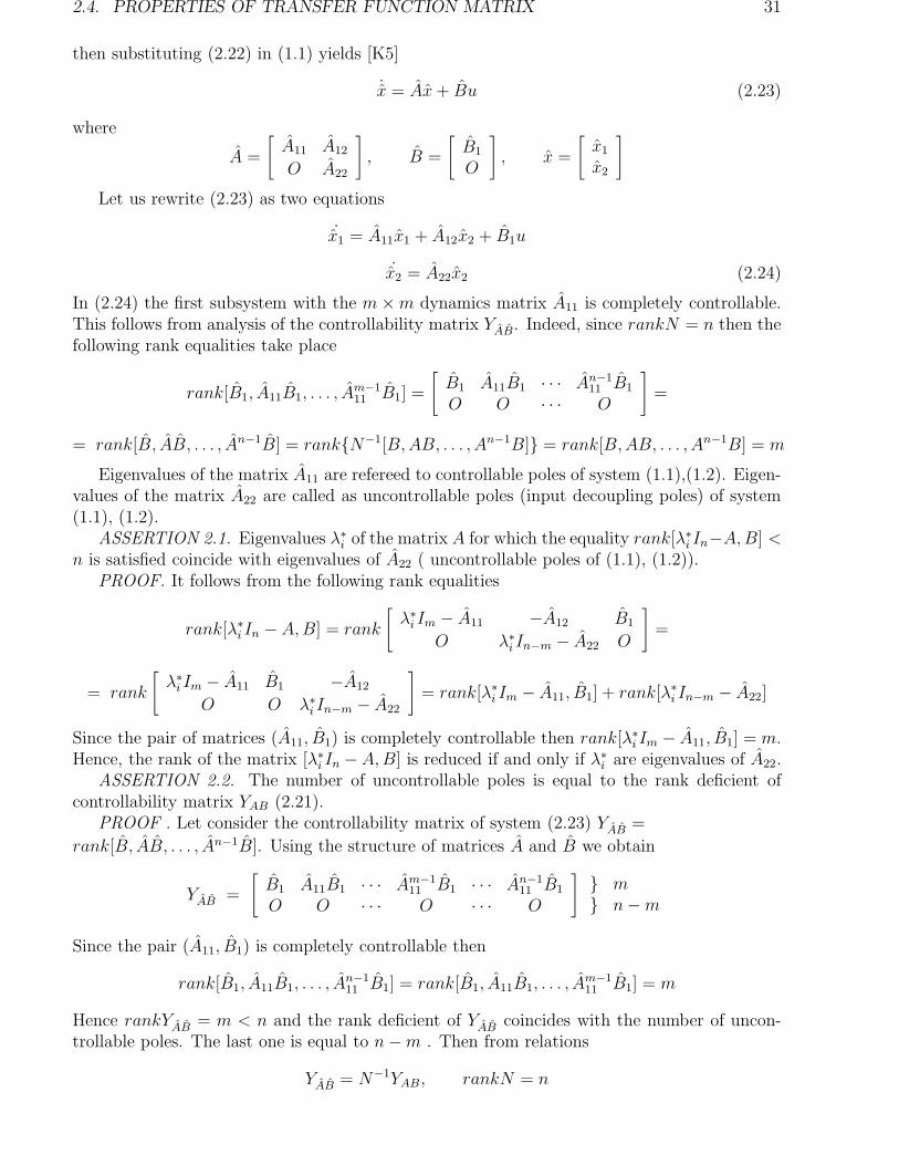
then substituting (2.22) in (1.1) yields [K5]
˙x = Ax+ Bu (2.23)
where
A =
[
A11 A12
O A22
]
, B =
[
B1
O
]
, x =
[
x1
x2
]
Let us rewrite (2.23) as two equations
˙x1 = A11x1 + A12x2 + B1u
˙x2 = A22x2 (2.24)
In (2.24) the first subsystem with the m×m dynamics matrix A11 is completely controllable.This follows from analysis of the controllability matrix YAB. Indeed, since rankN = n then thefollowing rank equalities take place
rank[B1, A11B1, . . . , Am−111 B1] =
[
B1 A11B1 · · · An−111 B1
O O · · · O
]
=
= rank[B, AB, . . . , An−1B] = rankN−1[B,AB, . . . , An−1B] = rank[B,AB, . . . , An−1B] = m
Eigenvalues of the matrix A11 are refereed to controllable poles of system (1.1),(1.2). Eigen-values of the matrix A22 are called as uncontrollable poles (input decoupling poles) of system(1.1), (1.2).
ASSERTION 2.1. Eigenvalues λ∗i of the matrix A for which the equality rank[λ∗i In−A,B] <n is satisfied coincide with eigenvalues of A22 ( uncontrollable poles of (1.1), (1.2)).
PROOF. It follows from the following rank equalities
rank[λ∗i In −A,B] = rank
[
λ∗i Im − A11 −A12 B1
O λ∗i In−m − A22 O
]
=
= rank
[
λ∗i Im − A11 B1 −A12
O O λ∗i In−m − A22
]
= rank[λ∗i Im − A11, B1] + rank[λ∗i In−m − A22]
Since the pair of matrices (A11, B1) is completely controllable then rank[λ∗i Im − A11, B1] = m.Hence, the rank of the matrix [λ∗i In −A,B] is reduced if and only if λ∗i are eigenvalues of A22.
ASSERTION 2.2. The number of uncontrollable poles is equal to the rank deficient ofcontrollability matrix YAB (2.21).
PROOF . Let consider the controllability matrix of system (2.23) YAB =
rank[B, AB, . . . , An−1B]. Using the structure of matrices A and B we obtain
YAB =
[
B1 A11B1 · · · Am−111 B1 · · · An−1
11 B1
O O · · · O · · · O
]
m n−m
Since the pair (A11, B1) is completely controllable then
rank[B1, A11B1, . . . , An−111 B1] = rank[B1, A11B1, . . . , A
m−111 B1] = m
Hence rankYAB = m < n and the rank deficient of YAB coincides with the number of uncon-trollable poles. The last one is equal to n−m . Then from relations
YAB = N−1YAB, rankN = n

32 CHAPTER 2. SYSTEM DESCRIPTION BY TRANSFER FUNCTION MATRIX
we haverankYAB = rank(N−1YAB) = rankYAB
The last equality completes the proof.Let’s find the output vector of the transformed system (2.23). As x = Nx then y = Cx =
CN−1x. We denote C = CN and rewrite the vector y as follows
y = Cx = CNx = CN1x1 + CN2x2 = C1x1 + C2x2 (2.25)
The following subsystems S1 and S2
S1 : ˙x1 = A11x1 + A12x2 + B1u, y1 = C1x1
S2 : ˙x2 = A22x2, y2 = C2x2
have properties: subsystem S1 is completely controllable and observable, subsystem S2 is un-controllable.
Now we find the transfer function matrix of system (2.23), (2.25)
G(s) = C(sI − A)−1B = CN
[
sI − A11 −A12
O sI − A22
] [
B1
O
]
Since for detA 6= 0, detC 6= 0
[
A −BO C
]−1
=
[
A−1 A−1BC−1
O C−1
]
then
G(s) = CN
[
(sIm − A11)−1 (sIm − A11)
−1A12(sIn−m − A22)−1
O (sIn−m − A22)−1
] [
B1
O
]
=
= [C1, C2]
[
(sIm − A11)−1B1
O
]
= C1(sIm − A11)−1B1
So, transfer function matrix G(s) coincides with one for the completely controllable subsys-tem S1. Since from Property 2.1 G(s) = G(s) then we have the following assertion.
ASSERTION 2.3. TFM of an uncontrollable and completely observable system coincideswith the TFM of the completely controllable and observable subsystem. Poles of TFM coincidewith controllable poles.
The analogous result can be obtained for a completely controllable and unobservable system.Such system is transformed into the following canonical form [K5]
˙x =
[
A11 O
A21 A22
]
x+
[
B1
B2
]
u,
y =[
C1 O]
x (2.26)
System (2.26) is decomposed into two subsystems
S1 : ˙x1 = A11x1 + B1u, y1 = C1x1
S2 : ˙x2 = A21x2 + A22x2 + B2u
with completely controllable and observable subsystem S1 and unobservable subsystem S2.Eigenvalues of the matrix A11 are named as observable poles. Eigenvalues of matrix A22 are

2.4. PROPERTIES OF TRANSFER FUNCTION MATRIX 33
named as unobservable poles (output decoupling poles). It can be shown that TFM of control-lable and unobservable system (1.1), (1.2) is
G(s) = C1(sIm − A11)−1B1
So, we have the following result.ASSERTION 2.4. TFM of an unobservable and completely controllable system coincides
with TFM of the completely controllable and observable subsystem. TFM poles coincide withobservable poles.
Similar to Assertions 2.1, 2.2 we can obtainASSERTION 2.5. Eigenvalues λ∗i of the matrix A for which the equality rank[λ∗i In −
AT , CT ] < n is satisfied coincide with eigenvalues of A22 (unobservable poles of (1.1),(1.2)).ASSERTION 2.6. A number of unobservable poles is equal to a rank deficient of the
unobservability matrix.Let’s consider uncontrollable and unobservable system (1.1), (1.2). Using a nonsingular
transformation of the state vector this system can be reduce to the following block form [K1]
˙x1
˙x2
˙x3
˙x4
=
A11 A12 A13 A14
O A22 A23 A24
O O A33 A34
O O O A44
x1
x2
x3
x4
+
B1
B2
OO
u,
y =[
O C2 O C4
]
x, xT = [xT1 , xT2 , x
T3 , x
T4 ] (2.27)
We may rewrite (2.27) as four connected subsystems
S1 : ˙x1 = A11x1 + A12x2 + A13x3 + A14x4 + B1u
S2 : ˙x2 = A22x2 + A23x3 + A24x4 + B2u, y1 = C2x2
S3 : ˙x3 = A33x3 + A34x4
S4 : ˙x4 = A44x4, y2 = C4x4
(2.28)
where S1 is completely controllable but unobservable, S2 is completely controllable and ob-servable, S3 is completely uncontrollable and unobservable, S4 is completely uncontrollablebut observable. Eigenvalues of the matrix A22 are simultaneously controllable and observablepoles. Eigenvalues of matrix A11 are unobservable poles (output decoupling poles). Eigenvaluesof matrix A44 are uncontrollable poles (input decoupling poles). Eigenvalues of matrix A33 aresimultaneously uncontrollable and unobservable poles (input - output decoupling poles).
Let’s find TFM of system (2.27). Using the block structure we can determine
G(s) = C2(sI − A22)−1B2 (2.29)
Since G(s) = G(s) then we obtain the assertion.ASSERTION 2.7. TFM of an incompletely controllable and observable system coincides
with TFM of the completely controllable and observable subsystem S2. Poles of TFM coincidewith simultaneously controllable and observable poles.
CONCLUSION
1. Poles of a completely controllable and observable system (1.1), (1.2) coincide witheigenvalues of the dynamics matrix A.
2. Poles of an incompletely controllable and/or observable system are eigenvalues ofthe dynamics matrix A without decoupling poles.
3. TFM of an incompletely controllable and observable system coincides with TFM ofa completely controllable and observable subsystem.

34 CHAPTER 2. SYSTEM DESCRIPTION BY TRANSFER FUNCTION MATRIX
2.5 Canonical forms of transfer function
matrix
2.5.1 Numerator of transfer function matrix
Let single-input/single-output system (1.1),(1.2) has a strictly proper scalar rational transferfunction
g(s) =ψ(s)
φ(s)
with ψ(s) and φ(s) relatively prime 2 polynomials in a complex variable s having real coefficients.Orders of ψ(s) and φ(s) are m and n respectively (m < n). Let’s present g(s) as
g(s) = ψ(s)[φ(s)]−1 = [φ(s)]−1ψ(s)
We may say that the transfer function g(s) is factorizated as the product of the polynomial ψ(s)and the inverse of the other polynomial φ(s). The polynomial ψ(s) is known as a numerator oftransfer function g(s).
We try to get the similar factorization of the strictly proper transfer function matrix G(s)with elements are strictly proper rational functions in a complex variable s with real coefficients.We need to factorizate G(s) into a product G(s) = C(s)P (s)−1 where C(s) and P (s) arerelatively prime polynomial matrices in s.3
At first we introduce some definitions. In the product P (s) = Q(s)R(s) a matrix R(s) iscalled a right divisor of the matrix P (s) and a matrix P (s) is called a left multiple of the matrixR(s)
DEFINITION 2.3. A square polynomial matrix D(s) is called as a common right divisorof matrices C(s) and P (s) if and only if
C(s) = C1(s)D(s), P (s) = P1(s)D(s) (2.30)
where C1(s), P1(s) are some polynomial matrices.DEFINITION 2.4. A square polynomial matrix D(s) is called as a greatest common right
divisor of matrices C(s) and P (s) if and only ifa) the matrix D(s) is the common right divisor of matrices C(s) and P (s),b) the matrix D(s) is the left multiple of every common right divisor of matrices C(s) and
P (s).Similarly we can define the greatest common left divisor of matrices C(s) and P (s).Let us consider the important particular case.DEFINITION 2.5. A square polynomial matrix U(s) is called as unimodular matrix if and
only if detU(s) is an nonzero scalar that independent in s.An inverse of the unimodular matrix is also a polynomial matrix.DEFINITION 2.6. Two polynomial matrices C(s) and P (s) are called as relatively right(left)
prime ones if a greatest common right (left) divisor of C(s) and P (s) is a unimodular matrix.THEOREM 2.1. [D2] Any proper l× r rational function matrix (having rational functions
as elements) always may be (nonuniquely) represented as the product
G(s) = C(s)P (s)−1 (2.31)
2The polynomials ψ(s) and φ(s) relatively prime if they have not any common multipliers being a polynomialin s.
3A polynomial matrix has polynomials in complex variable s as elements. We consider only polynomialswith real coefficients.

2.5. CANONICAL FORMS OF TRANSFER FUNCTION MATRIX 35
where C(s) and P (s) are relatively prime polynomial matrices of dimensions l × r and r × rrespectively.
The representation (2.31) is known as a factorization of a transfer function matrix G(s)[W1].
Similarly the matrix G(s) may be factorizated into a product of relatively left prime poly-nomial matrices N(s) and Q(s) of dimensions l × l and l × r respectively
G(s) = N(s)−1Q(s) (2.32)
It is significant that although matrices C(s) and P (s) in (2.31) are relatively prime butpolynomials detC(s) and detP (s) are not relatively prime for l = r. For example, this result isobserved for the following matrices [D2]
C(s) =
[
s− 1 00 s− 2
]
, P (s) =
[
s− 2 00 s− 1
]
DEFINITION 2.7. If polynomial matrices C(s) and P (s) in (2.31) are relatively right primethen an l × r polynomial matrix C(s) is called as a numerator of TFM G(s) [W2].
Similarly if polynomial matrices N(s) and Q(s) in (2.32) are relatively left prime then anl × r polynomial matrix Q(s) is called as a numerator of TFM .
In the following we will show that all numerators of any TFM can be transform into theuniquely standard canonical form. This canonical form is known as Smith’s form.
2.5.2 Smith form of numerator
For a polynomial matrix with real coefficients we introduce notions of elementary row (col-umn) operations [R1], [W1]:
1. interchanging any two rows(columns),2. multiplication any row (column) by a nonzero real scalar,3. Adding to any row (column) a product of any other row (column) by any polynomial or
real scalar.We need to note that an unimodular matrix is obtained from the identity matrix I by a
finite number of elementary row and column operations on I. Therefore, a determinant of anunimodular matrix is a nonzero scalar.
It follows from the definition of an unimodular matrix that any sequence of elementary row(column) operations on a polynomial matrix is equivalent to the premultiplication (postmulti-plication) this matrix by appropriate an unimodular matrix UL(s)(UR(s)). Such operations wewill call as equivalent operations.
DEFINITION 2.8. Two polynomial matrices P (s) and Q(s) will be called as equivalent
polynomial matrices if and only if the first one can be obtained from the second one by asequence of equivalent operations.
Equivalent polynomial matrices P (s) and Q(s) satisfy the following relation
P (s) = UL(s)Q(s)UR(s) (2.33)
where UL(s) and UR(s) are unimodular matrices.Since an unimodular matrix is nonsingular one then it follows from (2.33) that equivalent
operations do not change the rank of a polynomial matrix, i.e. rankP (s) = rankQ(s).Let’s consider reducing an l × r polynomial matrix P (s) of the rank m ≤ min(r, l) to the
Smith form [M1] (or normal form). We denote polynomial elements of the matrix P (s) by

36 CHAPTER 2. SYSTEM DESCRIPTION BY TRANSFER FUNCTION MATRIX
pij(s). Let pjd(s) and phk(s) are two nonzero elements. We need to show that if neither of theseelements is a divisor of the other, then carrying out only equivalent operations we can obtaina new matrix P1(s), which contains a nonzero element of lower degree than either pjd(s) orphk(s).
We will analyze the three cases:1. If pjd(s) and phk(s) are in the same column (d = k), and ρ(pjd(s)) ≤ ρ(phk(s)) where ρ
is a degree of a polynomial element, then subtracting g(s) times the j-th row of P (s) from theh-th row we obtain the following relation
phk(s) = g(s)pjk(s) + r(s)
where g(s) is a nonzero polynomial and r(s) is a polynomial with ρ(r(s)) < ρ(pjk(s)) or r(s) = 0.That is r(s) is the lowest degree polynomial remainder after division of the polynomial phk(s)by the polynomial g(s).
If we assume thata) pjk(s) and phk(s) are relatively primeb) ρ(pjk(s)) ≤ ρ(phk(s))then r(s) must be nonzero polynomial and ρ(r(s)) < ρ(phk(s)), ρ(r(s)) < ρ(pjk(s)). Therefore,using only equivalent operations we can decrease the degree of a element phk(s) changing thiselement by r(s), which is the remainder from the division phk(s) by pjk(s).
2. If pjd(s) and phk(s) are in the same row (h = j) then the similar procedure may beapplied where the role of a row/column is interchanged.
3. If k 6= d, h 6= j then the same procedure can be applied to both a row and a column bycomparing pjd(s) and phk(s) with a element phd(s).
Thus we has shownASSERTION 2.8. If pij(s) is the least degree element of P (s) and it does not divide every
element of P (s) then equivalent operations, as just consider, will lead to a new matrix P1(s)containing elements of lower degrees.
Carrying out this procedure many times we can obtain matrices Pi(s), i = 2, 3, . . . containingelements of more lower degrees. This process be finished after a finite number of steps since adegree of a polynomial is a finite positive integer.
Let’s suppose that the process is finished by a matrix P (s). We can permute rows andcolumns of P (s) until the element p11(s) becomes nonzero and of a least degree. Let emphasizethat p11(s) must divide every element of P (s). This important property of p11(s) follows fromconstructing matrices P1(s), P2(s),. . . , P (s). Indeed, let some pst(s) does not divided by p11(s)without a remainder. Then we can represent pst(s) as pst(s) = g(s)p11(s) + r(s) where r(s)is a polynomial with ρ(r(s)) ≤ ρ(pst(s)). Therefore, we obtain the contradiction with theassumption that the matrix P (s) has the element p11(s) of the least degree.
Taking into account this property of the element p11(s) and using elementary row (column)operations of the third type can reduce the matrix P (s) to the following matrix P1(s)
P1(s) =
p11(s)... 0 · · · 0
. . . . . . . . . .
0...
...... X(s)
0...
(2.34)
where X(s) is a some (l − 1) × (r − 1) polynomial submatrix.

2.5. CANONICAL FORMS OF TRANSFER FUNCTION MATRIX 37
Repeating the whole operation with the smaller matrix X(s) without changing the first rowor column of P1(s) we get the following matrix P2(s)
P2(s) =
p11(s) 0... 0 · · ·0
0 p22(s)... 0 · · ·0
. . . . . . . . . . . . . . .
0 0...
......
... X(s)
0 0...
(2.35)
Continuing this process we reduce finally the matrix P (s) to the form
S(s) =
s1(s) 0 · · · 0 · · · 00 s2(s) · · · 0 · · · 0...
......
...0 0 · · · sm(s) · · · 0...
......
...0 0 · · · 0 · · · 0
(2.36)
where m is a normal rank4 of the l × r polynomial matrix P (s) and every si(s) divides sj(s)without a remainder (i < j). Divisibility sj(s) by si(s) follows from the construction of thematrix S(s) because the element p11(s) divides all elements of X(s) and so on.
Since the matrix S(s) is resulted from the matrix P (s) by a sequence of equivalent operationswhich could be realized by unimodular matrices UL(s) and UR(s) (i.e. S(s) = UL(s)P (s)UR(s))then
rankS(s) = rankP (s) = m
The matrix S(s) (2.36) is known as the Smith canonical form for a polynomial matrix or theSmith form [L2].
2.5.3 Invariant polynomials
Now we show that only equivalent polynomial matrices may be reduced to identical Smithforms. Let a polynomial matrix P (s) has a normal rank m ≤ min(r, l). A greatest commondivisor of all j-th order minors (j = 1, 2, . . . , m) of P (s) we denote by dj(s). Since any j-thorder minor (j > 2) would be expressed as a linear combination of (j − 1)-th order minorsthen dj−1(s) is the divisor of dj(s). If we denote do(s) = 1 then every dj(s) is divided bydj−1(s), j = 1, . . . , m in the sequence do(s), d1(s), . . . , dm(s). We define
ǫm(s) =dm(s)
dm−1(s), ǫm−1(s) =
dm−1(s)
dm−2(s), · · · , ǫ1(s) =
d1(s)
do(s)(2.37)
Polynomials ǫ1(s), . . . , ǫm(s) are called as invariant polynomials of P (s). It can be shown thesepolynomials are invariants under equivalent operations.
ASSERTION 2.9. Two equivalent polynomial matrices P (s) and Q(s) have equal invariantpolynomials.
4The normal rank (or rank) of a polynomial matrix is the order of the largest minor, which is not identicallyzero [B2]

38 CHAPTER 2. SYSTEM DESCRIPTION BY TRANSFER FUNCTION MATRIX
PROOF. If two matrices P (s) and Q(s) are equivalent then two unimodular matrices UL(s)and UR(s) exist such that Q(s) = UL(s)P (s)UR(s). Unimodular matrices UL(s) and UR(s)have nonzero scalar determinants then rankQ(s) = rankP (s). Let’s denote greatest commondivisors of all j-th order minors of matrices P (s) and Q(s) by dk(s) and δk(s) respectively. Fromthe equality Q(s) = UL(s)P (s)UR(s) we obtain that every k-th order minor (1 ≤ k ≤ m) ofthe matrix Q(s) should be expressed by the formula Caushy-Binet [G1] as a linear combinationof k-th order minors of P (s). Hence δk(s) is divided by dk(s). Vise versa: from the equalityP (s) = UL(s)−1Q(s)UR(s)−1 it follows divisibility of dk(s) by δk(s). That is why
dk(s) = δk(s), k = 1, . . . , n
Consequently P (s) and Q(s) have equal invariant polynomials. This completes the proof.
Let us calculate invariant polynomials of the matrix S(s) (2.36). Since
d1(s) = s1(s), d2(s) = s1(s)s2(s), . . . , dm(s) = s1(s)s2(s) · · · sm(s)
then we have from (2.37)
ǫm(s) = sm(s), ǫm−1(s) = sm−1(s), . . . , ǫ1(s) = s1(s) (2.38)
Hence, diagonal elements of the Smith form coincide with invariant polynomials of S(s).
As the matrix S(s) is obtained from the matrix P (s) by the sequence of equivalent operationsthen these matrices are equivalent and have similar invariant polynomials. The last follows fromAssertion 2.9. We have obtained the following assertion.
ASSERTION 2.10. Any polynomial matrix P (s) is reduced to Smith form (2.36) withdiagonal elements si(s) that are invariant polynomials of P (s) .
Since any two equivalent polynomial matrices have equal invariant polynomials then thefollowing corollary is true.
COROLLARY 2.1. Any two polynomial matrices have the unique Smith form.
Let us consider two any numerators P (s) and Q(s) of a proper transfer function matrixG(s). It is evident that P (s) and Q(s) are l × r polynomial matrices. As it has been shownin [W2] if P (s) and Q(s) are two numerators of a rational function matrix G(s) then they areequivalent. This means that polynomial matrices P (s) and Q(s) satisfy the relation (2.33) andby Corollary 2.1 they have the unique Smith form and equal invariant polynomials.
So, we conclude that all numerators of TFM G(s) have equal invariant polynomials andmay be reduced to the unique Smith canonical form.
EXAMPLE 2.1.
Let’s calculate the Smith form of the following matrix
P (s) =
s 0 00 s s+ 1s s− 1 0
(2.39)
Here r = l = 3 and m = rankP (s) = 3.
At first we construct the matrix P1(s) (2.24) by subtracting the second row of the matrix(2.39) from the third one
P1(s) =
s 0 00 s s+ 1s −1 −s− 1

2.5. CANONICAL FORMS OF TRANSFER FUNCTION MATRIX 39
Interchanging rows and columns in P1(s) we can reduce it to the following form with p11(s) = −1
P1(s) =
−1 s −s− 1s 0 s+ 10 s 0
Using the second and third types elementary operations we obtain the matrix P1(s) in the form(2.34)
P1(s) =
−1... 0 0
. . . . . . . .
0... X(s)
0...
(2.40)
with
X(s) =
[
s2 −s2 + 1s 0
]
Adding the first column to second one in X(s) and interchanging columns obtained we resultin
X1(s) =
[
1 s2
s s
]
Using the third and second type elementary operations we transform X1(s) into the form (2.34)
X1(s) =
[
1 0s s(s2 − 1)
]
So, we have reduced the matrix P1(s) to the following one
P2(s) =
1 0 00 1 00 0 s(s2 − 1)
(2.41)
This matrix has the Smith form (2.36) with s1(s) = 1, s2(s) = 1, s3(s) = s(s2 − 1).For checking we calculate invariant polynomials of the matrix (2.39). It has three nonzero
first order minors: s, s − 1, s + 1 with the great common divisor d1(s) = 1, four nonzerosecond order minors: s2, s(s + 1), s(s − 1), (s + 1)(s − 1) with the great common divisord2(s) = 1 and one third order nonzero minor d3(s) = s(s−1)(s+1). Using (2.37) we determineinvariant polynomials
ǫ3(s) =d3(s)
d2(s)= s(s2 − 1), ǫ2(s) =
d2(s)
d1(s)= 1, ǫ1(s) =
d1(s)
do(s)= 1
So, invariant polynomials of P (s) coincide with diagonal elements of the form (2.41). Thisresult is adjusted with Assertion 2.10.
2.5.4 Smith-McMillan form of transfer function matrix
Now we demonstrate that the canonical form of a rational function matrix (the Smith-McMillan canonical form) can be obtained by using the Smith canonical form. We considerany l×r rational function matrix W (s) having a rank m ≤ min(r, l). Let a polynomial φ(s) is a

40 CHAPTER 2. SYSTEM DESCRIPTION BY TRANSFER FUNCTION MATRIX
monic least common denominator of all elements ofW (s). We form the matrix T (s) = φ(s)W (s)that is a polynomial l × r matrix. Let ST (s) is the Smith form of the matrix T (s), i.e.
ST (s) = UL(s)T (s)UR(s) (2.42)
where UL(s) and UR(s) are unimodular l× l and r× r matrices respectively and ST (s) has thefollowing structure
ST (s) =
diagsT1(s), sT2(s), . . . , sTm(s) ... O. . . . . . . . . . . . . . . . . . . . . . . . . . . . . . . . . .
O... O
(2.43)
where sT i(s) are invariant polynomials of T (s) . Since T (s) = φ(s)W (s) then dividing bothleft-hand and right-hand sides of (2.42) by φ(s) (s 6= si, si is a zero of φ(s)) yields
ST (s)
φ(s)= UL(s)W (s)UR(s) (2.44)
To discover a structure of ST (s)/φ(s) we use (2.43)
ST (s)
φ(s)=
diag sT1(s)φ(s)
, sT2(s)φ(s)
, . . . , sTm(s)φ(s)
... O
. . . . . . . . . . . . . . . . . . . . . . . . . . . . . . .
O... O
(2.45)
Since elements sT i(s), i = 1, 2, . . . , m are invariant polynomials of T (s) then they satisfy thefollowing condition: sT i(s) is divided by sT,i−1(s) without a remainder. Therefore, elementssT i(s)/φ(s) satisfy the same requirement. Carrying out all possible cancellations in sT i(s)/φ(s)we result in a ratio of two monic polynomials ǫi(s)/ψi(s), which have to satisfy conditions:
ǫi(s)
ψi(s)must divide
ǫi+1(s)
ψi+1(s), i = 1 , . . . ,m − 1 (2.46)
It follows from (2.46) that
ǫi(s) must divide ǫi+1(s) i = 1 , . . . ,m − 1 (2.47)
ψi+1(s) must divide ψi(s), i = 1 , . . . ,m − 1 , ψ1 (s) = φ(s) (2.48)
Denoting M(s) = ST (s)/φ(s) we obtain from (2.45) and the last relation
M(s) =
diag ǫ1(s)ψ1(s)
, ǫ2(s)φ2(s)
, . . . , ǫm(s)φm(s)
... O
. . . . . . . . . . . . . . . . . . . . . . . . . . . . .
O... O
(2.49)
This matrix is known as the Smith-McMillan canonical form of a rational function matrix W (s).Using (2.44) we can write
M(s) = UL(s)W (s)UR(s) (2.50)
Thus, a rational function matrix W (s) is reduced to the Smith-McMillan canonical form by thesequence of elementary operations.

2.5. CANONICAL FORMS OF TRANSFER FUNCTION MATRIX 41
EXAMPLE 2.2 [S14]Let a 4 × 3 transfer function matrix has the form
W (s) =
1s(s+1)2
s2+2s−1s(s+1)2
s+2s−2
0 s+2(s+1)2
0
0 0 3(s+2)s+1
s+3s(s+1)2
2s2+3s+3s(s+1)2
s+2s−2
(2.51)
We calculate the least common denominator of all elements of W (s) : φ(s) = s(s + 1)2 andform the matrix T (s) = φ(s)W (s)
T (s) =
1 s2 + 2s− 1 (s+ 2)s(s+ 1)
0 s(s+ 2) 0
0 0 3s(s+ 1)(s+ 2)
s + 3 2s2 + 3s− 3 s(s+ 1)(s+ 2)
Let’s find the Smith form of T (s). By (2.36) we need to know invariant polynomials ǫi(s) =sT i(s) of T (s). For this we calculate a greatest common divisor di(s) of the i order minors(i = 1, 2, 3) of the matrix T (s): do = 1, d1(s) = 1, d2(s) = s(s + 2), d3(s) = s2(s + 1)(s + 2)2
and using (2.37) find
sT1(s) =d1(s)
d0(s)= 1, sT2(s) =
d2(s)
d1(s)= s(s+ 2), sT3(s) =
d3(s)
d2(s)= s(s+ 1)(s+ 2)
Thus, the Smith form ST (s) of the matrix T (s) is
ST (s) =
1 0 0
0 s(s+ 2) 0
0 0 s(s+ 1)(s+ 2)
0 0 0
Calculating ǫi(s)/ψi(s) = sT i(s)/φ(s) with φ(s) = s(s+ 1)2
ǫ1(s)
ψ1(s)=sT1(s)
φ(s)=
1
s(s+ 1)2,
ǫ2(s)
ψ2(s)=sT2(s)
φ(s)=
s+ 2
(s+ 1)2,
ǫ3(s)
ψ3(s)=sT3(s)
φ(s)=
s+ 2
(s+ 1)
and using the formula (2.49) we obtain the matrix M(s) being the Smith-McMillan form ofW (s)
M(s) =
1s(s+1)2
0 0
0 s+2(s+1)2
0
0 0 s+2s+1
0 0 0
(2.52)

42 CHAPTER 2. SYSTEM DESCRIPTION BY TRANSFER FUNCTION MATRIX
Now we reveal the relationship between the matrix M(s) and the Smith canonical form ofany l×r numerator of a transfer function matrix of a rankm. For simplicity we letm = min(r, l)and denote
E(s) = diag(ǫ1(s), ǫ2(s), . . . , ǫm(s))
Ψ(s) = diag(ψ1(s), ψ2(s), . . . , ψm(s)) (2.53)
Using (2.53) we can present the matrix M(s) (2.49) as
M(s) = E(s)Ψ(s)−1 = Ψ(s)−1E(s) (2.54)
Thus, we obtain that the Smith-McMillan form of a rational function matrix M(s) is factorizedinto the product of the l × r polynomial matrix E(s) and an inverse of the r × r polynomialmatrix Ψ(s). Matrices E(s) and Ψ(s) are the relatively right prime ones andE(s) is a numeratorof the rational function matrix M(s). The matrix E(s) is in the Smith form that is unique onefor all numerators of TFM (2.51) by Corollary 2.1.
CONCLUSION
Polynomials ǫi(s) of the Smith-McMillan can be calculated by the factorization of TFM intoa product of relatively prime polynomial matrices and following calculating the Smith form ofthe numerator.

Chapter 3
Notions of transmission and invariantzeros
3.1 Classic definition of zeros
Let’s consider system (1.1), (1.2) with a single input and single output (r = l = 1). Thetransfer function of this system is defined from formula (2.7) as
g(s) = c(sIn − A)−1b (3.1)
where c is an n-dimensional row vector, b is an n-dimensional column vector. We propose thatsystem (1.1),(1.2) is completely controllable and observable. Then its a transfer function g(s)is the ratio of two relatively prime polynomials
g(s) =ψ(s)
φ(s)(3.2)
where φ(s) = det(sIn − A) is a polynomial of order n with zeros λ1, λ2, . . . , λn being poles ofg(s) and ψ(s) = c(adj(sIn − A))b is a polynomial of order m < n. Zeros z1, z2, . . . , zm of ψ(s)are called as zeros of the scalar transfer function (TF) g(s). Since g(s) is an irreducible rationalfunction then λi 6= zj (i = 1, 2, . . . , n; j = 1, 2, . . . , m).
Now we study the physical interpretation of zeros of TF. Let a scalar exponential signal isapplied at the input of system (1.1),(1.2)
u(t) = uo exp(jwt)1(t), t > 0 (3.3)
where jw is a complex frequency, w is a real value, uo 6= 0 is a scalar constant value, 1(t) is theunit step function1. According to formulas (2.14),(3.2) we obtain the following output responsefor x(to) = 0
y(t) ∼= g(jwt)u(t) =ψ(jw)
φ(jw)uo exp(jwt) (3.4)
It is follows from (3.4) that ψ(jw) = 0 (φ(jw) 6= 0) if the complex frequency jw coincides witha certain zero zi of g(s). In this case the output response be trivial (identically zero).
So, we conclude: In the classic single input/output controllable and observable system atransmission zero is defined as a value of a complex frequency s = zi at which the transmission
11(t) =
0, if t ≤ 01, if t > 0
43

44 CHAPTER 3. NOTIONS OF TRANSMISSION AND INVARIANT ZEROS
of the exponential signal exp(zit) is blocked. It is evident that the transmission zero coincidesis any zero of the numerator of the transfer function g(s).
Similarly we may define a transmission zero of a linear multivariable system (having a vectorinput/output) as a complex frequency at which the transmission of a signal is ’blocked’. In thefollowing section we will define transmission zeros via the transfer function matrix G(s).
3.2 Definition of transmission zero via transfer function
matrix
Lets’s consider completely controllable and observable system (1.1), (1.2) with r inputs andl outputs (r, l > 1). The transfer function matrix G(s) of this system is a rational functionmatrix with elements being rational irreducible scalar functions. We propose that l ≥ r andrankG(s) = min(r, l) = r. Let a exponential signal
u(t) = uo exp(jwt)1(t), t > 0 (3.5)
is applied at the input of (1.1),(1.2). In (3.5) jw is a complex frequency, w is a real value,uo 6= 0 is a nonzero constant r vector. According to formula (2.14) we can write the followingoutput steady response for x(to) = O
y(t) ∼= G(jwt)u(t) = G(jw)uo exp(jwt) (3.6)
We assume that jw 6= λi where λi (i = 1, 2, . . . , n) are poles of the system, which coincide withzeros of the polynomial φ(s) = det(sIn − A) for the completely controllable and observablesystem.
If the rank of G(s) is locally reduced at s = jw then a nonzero constant r vector v exists,which is a nontrivial solution of the linear system
G(jw)v = O (3.7)
Setting uo = v in (3.5) and taking into account (3.7) we have y(t) = G(jw)v exp(jwt) = O.This fact means that there exists the exponential input vector (3.5) of a corresponding complexfrequency jw such that the output steady response is identically zero. The value of a complexfrequency s = jw that locally reduces the rank of G(s) is the transmission zero.
DEFINITION 3.1. A complex frequency s = z at which a rank of the transfer functionmatrix is locally reduced
rankG(s)/s=z < min(r, l) (3.8)
is called as a transmission zero.Thus, if a complex frequency s coincides with a transmission zero z of a multi-input/multi-
output system then there exists some nonzero proportional exp(zt) input vector such that itspropagating through the system is blocked.
Let’s consider the difference between the multi-input/multi-output case and the classic one.The scalar transfer function g(s) vanishes at s = z in the single-input/single-output case, thenany proportional exp(zt) input signal does not transmit through the system (’blocked’). In themulti-input/multi-output case the transfer function matrix does not become the zero matrixat s = z but its the rank is locally reduced. This fact means that there exists a nonzeroproportional exp(zt) input vector signal, which may propagate through the system.
REMARK 3.1. The inequality (3.8) for l ≥ r is the necessary and sufficient condition for’blocking’ the transmission of a exponential signal. It is only sufficient condition for r > l.

3.2. DEFINITION OF TRANSMISSION ZERO VIA TRANSFER FUNCTION MATRIX 45
Namely, if the condition (3.8) is satisfied for s = z then there always exists a proportional toexp(zt) input signal such that y(t) = O, t ≫ 0. The inverse proposition ( if y(t) = O for aproportional exp(zt) input signal then rankG(s) < l) is not true. Indeed, consider the following2 × 3 transfer function matrix
G(s) =1
(s+ 1)(s+ 2)
[
s 0 s0 s− 0.5 0
]
of the normal rank 2. The steady response y(t) to the input signal u(t) = [1, 0,−1]T expjwt 1(t)(w 6=0) is defined by formula (3.6)
y(t) =1
(jw + 1)(jw + 2)
[
jw 0 jw0 jw − 0.5 0
]
10
−1
exp(jwt) =
[
00
]
Hence the steady response is equal to zero although the rank of G(s)/s=jw is not reduced.The following simple example illustrates blocking an oscillatory input signal of the frequency
coincided with a transmission zero.EXAMPLE 3.1.
Let completely controllable and observable system (1.1),(1.2) with n = 3, l = r = 2 has thetransfer function matrix
G(s) =1
(s+ 1)(s+ 2)(s+ 3)
[
s2 + 0.25 00 1
]
(3.9)
One can see that the rank of G(s) is reduced at s = ±0.5j. Let’s inject in the system thefollowing oscillatory signal of frequency 0.5
u(t) =
[
v1
v2
]
2cos(0.5t), v1 6= v2 6= 0
This signal can be represented as the sum of two complex exponential signals
u(t) =
[
v1
v2
]
2cos(0.5t) =
[
v1
v2
]
(exp(0.5jt) + exp(0.5jt)) = u1(t) + u2(t)
Using formula (3.6) we find the output steady response to zero initial conditions
y(t) = y1(t) + y2(t) = G(0.5j)u1(t) +G(−0.5j)u2(t) =
=1
(0.5j + 1)(0.5j + 2)(0.5j + 3)
[
0 00 1
] [
v1
v2
]
exp(0.5jt)+
+1
(−0.5j + 1)(−0.5j + 2)(−0.5j + 3)
[
0 00 1
] [
v1
v2
]
exp(−0.5jt)
It is easy to verify that y(t) ≡ O for v1 = q 6= 0, v2 = 0 where q is any constant value. Thisfact means that the steady output response to the nonzero input signal
u(t) =
[
2q0
]
2cos(0.5t)
is the identically zero.

46 CHAPTER 3. NOTIONS OF TRANSMISSION AND INVARIANT ZEROS
3.3 Transmission zero and system response
Now we consider the output response of system (1.1),(1.2) with the nonzero initial statex(to) 6= O. We assume that matrix A has n distinct eigenvalues λ1, . . . , λn. Let’s apply thefollowing the exponential type input
u(t) = uo exp(α∗t)1(t) (3.10)
where uo 6= O is a constant r vector, α∗ 6= λi, i = 1, . . . , n is a complex number. Substituting(3.10) in formula (1.9) (see Sec 1.1) and assuming to = 0 yields
y(t) =n∑
i=1
γi exp(λit)vTi xo +
n∑
i=1
γi
∫ t
0exp(λi(t− τ))βTi uo exp(α∗τ)dτ
where γi = Cwi, βTi = vTi B, xo = x(to) = 0.Taking out from the integral the terms that independent on τ
y(t) =n∑
i=1
γi exp(λit)vTi xo +
n∑
i=1
γiβTi uo exp(λit)
∫ t
0exp((α∗ − λi)τ)dτ
and integrating we obtain
y(t) =n∑
i=1
γi exp(λit)vTi xo +
n∑
i=1
γiβTi uo exp(λit)
α∗ − λi(exp((α∗ − λi)t) − 1) =
=n∑
i=1
γi exp(λit)vTi xo +
n∑
i=1
γiβTi uo
α∗ − λi(exp(α∗t) − exp(λit)) =
=n∑
i=1
γi exp(λit)vTi xo−
n∑
i=1
γiβTi uo
α∗ − λiexp(λit)+
n∑
i=1
γiβTi uo
α∗ − λiexp(α∗t) = yo(t)+y1(t)+y2(t) (3.11)
The analysis of this expression shows that the response y(t) is the sum of the following com-ponents: the response to the initial conditions yo(t), the term associated with the free motiony1(t) and the forced response y2(t). If all λi have negative real part then y(t) → y2(t) as t→ ∞.For small time y(t) depends on yo(t), y1(t) and y2(t).
We always may choose vector xo such that the components yo(t) and y1(t) are mutualeliminated. Indeed, from the equation
yo(t) + y1(t) =n∑
i=1
γi exp(λit)vTi xo −
n∑
i=1
γiexp(λit)v
Ti
α∗ − λiBuo = O
we can write
vTi xo =vTi
α∗ − λiBuo
Changing i from 1 to n and denoting V = [v1, v2, . . . , vn] we obtain the system of linear equationsin xo
V Txo = diag(α∗ − λ1, α∗ − λ2, . . . , α
∗ − λn)−1V TBuo
from which xo is calculated as
xo = (V T )−1diag(α∗ − λ1, α∗ − λ2, . . . , α
∗ − λn)−1V TBuo

3.3. TRANSMISSION ZERO AND SYSTEM RESPONSE 47
Since (V T )−1 = W where the matrix W consists of right eigenvectors wi (W = [w1, w2, . . . , wn])then the right-hand side of the last expression becomes
Wdiag(α∗ − λ1, α∗ − λ2, . . . , α
∗ − λn)−1V TBuo = (α∗In − A)−1Buo (3.12)
andxo = (α∗In − A)−1Buo (3.13)
Substituting this xo in (3.11) we obtain the output response containing only the forced response
y(t) = y2(t) =n∑
i=1
γiβTi
α∗ − λiuo exp(α∗t) (3.14a)
Using notions (1.10) ( γi = Cwi, βTi = vTi B) and the relation (3.12) we can rewrite (3.14a) as
y2(t) = C[w1, w2, . . . , wn]diag(α∗ − λ1, α
∗ − λ2, . . . , α∗ − λn)
−1[v1, v2, . . . , vn]TBuo exp(α∗t) =
= CWdiag(α∗ − λ1, α∗ − λ2, . . . , α
∗ − λn)−1V TBuo exp(α∗t) = C(α∗In − A)−1Buo exp(α∗t)
Since C(α∗In −A)−1B is the transfer function matrix of system (1.1),(1.2) at s = α∗ then
y2(t) = G(α∗)uo exp(α∗t) (3.14b)
If the complex frequency α∗ coincides with a transmission zero then the rank of G(α∗) isreduced and there exists a nonzero vector uo such as y2(t) ≡ O.
So, it has been shown: if α∗ is a transmission zero then there exists a nonzero vector uo anda nonzero initial state condition xo(α
∗In − A)−1Buo such as the output response to the input(3.10) is identically zero, i.e. y(t) = yo(t) + y1(t) + y2(t) ≡ O.
CONCLUSION
If a proportional exp(α∗t) signal is applied to an input of a completely controllable andobservable system where α∗ is a transmission zero, α∗ 6= λi ( distinct eigenvalues of A) then
a. there exists an initial state conditions xo such that the transmission of this signal throughthe system is blocked: y(t) ≡ O,
b. for x(t0) 6= xo 6= O the output response y(t) consists of the sum y0(t) + y1(t); thetransmission of forced response y2(t) is blocked,
c. for x(t0) 6= xo = O the output response y(t) contains only the free motion term y1(t); thetransmission of forced response y2(t) is blocked.
For the illustration we consider the following example.EXAMPLE 3.2.
Let’s completely controllable and observable system (1.1),(1.2) with n = 3, r = l = 2 hasthe following matrices A, B, C
A =
0 1 00 0 1
−6 −11 −6
, B =
−1 00 00 −1
, C =
[
0 −1 1−1 −1 0
]
Poles of this system coincide with eigenvalues of A: λ1 = −1, λ2 = −2, λ3 = −3. At first wefind eigenvectors wi and vTi , i = 1, 2, 3. Since A has distinct eigenvalues then the matrix W isthe Vandermonde matrix of the structure
W = [w1, w2, w3] =
1 1 1λ1 λ2 λ3
λ21 λ2
2 λ23
=
1 1 1−1 −2 −3
1 4 9

48 CHAPTER 3. NOTIONS OF TRANSMISSION AND INVARIANT ZEROS
Determining the matrix
V T = W−1 =
vT1vT2vT3
=
3 2.5 0.5−3 −4 −1
1 1.5 0.5
and vectors γi = Cwi, βTi = vTi B, i = 1, 2, 3
[γ1, γ2, γ3] = C[w1, w2, w3] =
[
0 −1 1−1 −1 0
]
1 1 1−1 −2 −3
1 4 9
=
[
2 6 120 1 2
]
,
βT1βT2βT3
=
vT1vT2vT3
B =
3 2.5 0.5−3 −4 −1
1 1.5 0.5
−1 00 00 −1
=
−3 −0.53 1
−1 −0.5
and using formulas (3.14a),(3.14b) we calculate the transfer function matrix G(s) at s = 1
G(1) =3∑
i=1
γiβTi
1 − λi= [γ1, γ2, γ3]diag(1 − λ1, 1 − λ2, 1 − λ3)
−1
βT1βT2βT3
=
=
[
2 6 120 1 2
]
0.5 0 00 0.33 00 0 0.25
−3 −0.53 1
−1 −0.5
=
[
0 012
112
]
Since the rank of the matrix G(s) is reduced at s = 1 then this frequency s is the transmissionzero.
Then we find the forced response y2(t) to the input signal
u(t) =
[
v−6v
]
exp(1t), v 6= O (3.15)
as follows
y2(t) = G(1)u(t) =
[
0 012
112
] [
v−6v
]
exp(1t) ≡ 0
and evaluate the free motion component
y1(t) =
[
2 6 120 1 2
]
0.5 exp(−t) 0 00 0.33 exp(−2t) 00 0 0.25 exp(−3t)
−3 −0.53 1
−1 −0.5
[
v−6v
]
=
=
[
−6 exp(−2t) + 6 exp(−3t)−6 exp(−2t) + exp(−3t)
]
v
We can see that y1(t) → O as t→ ∞. Hence, if the initial state condition is zero (x0 = O) thenthe output response y(t) = y1(t)+y(2(t) → O as t→ ∞. We have been observed the interestingphenomenon: the growing signal (3.15) is applied to the system input but the output response isvanished. This phenomenon is stipulated by coincidence of the input signal frequency with thetransmission zero. If xo 6= O eliminates free motion component y1(t) then the output responseremains zero even for a small t.

3.4. DEFINITION OF INVARIANT ZERO BY STATE-SPACE REPRESENTATION 49
3.4 Definition of invariant zero by state-space represen-
tation
Formerly we have been shown that a transmission zero is defined via the transfer functionmatrix G(s) of the completely controllable and observable system.
Let’s consider an incomplete controllable and/or observable system described in the state-space by linear differential equations (1.1),(1.2). We will study a response to the input signal
u(t) = uo exp(α∗t)1(t) (3.16)
and demonstrate that if α∗ is an invariant zero then the output response to (3.16) may be zero
y(t) = O, t > 0 (3.17)
for the following state motionx(t) = xo exp(α∗t)1(t) (3.18)
namely, we show that the invariant zero coincides with a frequency s = α∗ at which thetransmission of the exponential signal exp(α∗t) through the system is blocked.
At first we show that an invariant zero associates with reducing a rank of the (n+ l)×(n+r)system matrix [R1]
P (s) =
[
sIn − A −BC O
]
(3.19)
Taking the Laplace transform of (1.1), (1.2) and expressing x(s) via u(s) we get
y(s) = C(sIn −A)−1xo + C(sIn −A)−1Bu(s)
For a proper system the following equalities are follows from y(t) = O
y(to) = O or Cxo = O (3.20)
y(s) = O (3.21)
Substituting y(s) in (3.21) we obtain the relation
C(sIn −A)−1xo +Bu(s)) = O (3.22)
which using
u(s) =uo
s− α∗(3.23)
can be rewritten for s 6= α∗ (3.22) as follows
C(sIn −A)−1(s− α∗)xo +Buo = O (3.24)
Applying the obviously identity
(s− α∗)In = (sIn − A) − (α∗In − A) (3.25)
to (3.24) we obtain series of equalities
C(sIn − A)−1((sIn − A) − (α∗In − A))xo +Buo =
= C(sIn − A)−1(−(α∗In −A)xo +Buo) + C(sIn − A)−1(sIn − A)xo =

50 CHAPTER 3. NOTIONS OF TRANSMISSION AND INVARIANT ZEROS
= C(sIn −A)−1(−(α∗In − A)xo +Buo) + Cxo = O
that can be written for Cxo = O (see (3.20)) as
C(sIn − A)−1((α∗In −A)xo − Buo) = O (3.26)
Since the multiplier (α∗In − A)xo −Buo is independent on s then the following condition
(α∗In −A)xo − Buo = O (3.27)
is the necessary one to fulfilling (3.26) for any s. Uniting (3.20) and (3.27) we obtain theequality
[
sIn −A −BC O
] [
xouo
]
= O (3.28)
that is a necessary condition for existence of α∗, xo, uo such that y(t) = O.Let’s consider relation (3.28) as a linear matrix equation in the vector [xTo , u
To ]. It has a
nontrivial solution if a rank of the matrix
P (α∗) =
[
α∗In − A −BC O
]
is smaller then min(n+ r, n+ l) (it is the necessary and sufficient condition for l ≥ r and onlythe sufficient one for l < r). Therefore, for l ≥ r the column rank reduction of the matrixP (α∗)ensures existence of nonzero vectors xo and/or uo such that the transmission of the signal (3.16)through the system is blocked: y(t) = O. The corresponding nonzero initial state xo is definedfor s 6= α∗ from (3.27) as
xo = (α∗In − A)−1Buo (3.29)
Then from (2.3) and (3.23) we calculate the state response x
x(s) = (sIn −A)−1(xo +Buos− α∗
) =1
s− α∗(sIn −A)−1((s− α∗)xo +Buo)
that can be presented by using identity (3.25) as
x(s) =1
s− α∗(sIn −A)−1((−α∗In − A)xo +Buo) + xo
Then from (3.27) we find obtain x
x(s) =xo
s− α∗(3.30)
that is transformed by the inverse Laplace into the form
x(t) = xo exp(α∗t), t > 0
Thus, the state vector is the nonzero exponential vector of the frequency coincided with theinput signal frequency.
The condition (3.28) is also the sufficient one for existence of α∗, xo and uo such thaty(t) ≡ O because all steps of the proof can be reversed [M1]. So, it has been stated: to blockthe transmission of a proportional exp(α∗t) signal it is necessary and sufficient that a rank ofthe matrix P (s) is locally reduced at s = α∗.
DEFINITION 3.2. A complex frequency s = α∗ at which the column rank of P (s) is locallyreduced
rankP (s)/s=α∗ < min(n + r, n+ l) (3.31)

3.4. DEFINITION OF INVARIANT ZERO BY STATE-SPACE REPRESENTATION 51
is called as an invariant zero [M1].EXAMPLE 3.3.
Let’s calculate an invariant zero of the following system with n = 2, r = l = 1
x =
[
2 01 1
]
x+
[
10
]
u, y =[
1 1]
x (3.32)
This system is controllable and observable and has two poles λ1 = 1, λ2 = 2. Constructing the3 × 3 system matrix (3.19)
P (s) =
[
sI2 −A −BC O
]
=
s− 2 0 −1−1 s− 1 01 1 0
we reveal that the column (and row) rank of P (s) is locally reduced from 3 to 2 at s = 0.Hence, α∗ = 0 is the invariant zero. From equation (3.28) with α∗ = 0
−2 0 −1−1 −1 0
1 1 0
x10
x20
uo
= O
we find the vector xT0 = [x10, x20, uo] with xTo = [1, 1], u0 = −2. So, if the nonzero signalu(t) = −2 exp0 1(t) = 2 · 1(t) is applied in the input of system (3.32) then the output responseis zero for initial conditions x1(0) = 1, x2(0) = −1.
REMARK 3.1. The vector x0 calculating from (3.27) coincides with (3.13). Therefore,condition (3.28) generalizes conditions (3.8) and (3.13) to an incomplete controllable and/orobservable system with the matrix A of a general structure and without the restriction: α∗ 6= λi.
ASSERTION 3.1. If α∗ 6= λi(A) is a transmission zero then it is an invariant zero, theconverse is not true.
PROOF. Let α∗ is a transmission zero that satisfies condition (3.8). If system (1.1), (1.2) iscompletely controllable and observable then its TFM is G(s) = C(sIn−A)−1B, otherwise TFMof (1.1),(1.2) coincides with TFM of the completely controllable and observable subsystem.Transmission properties of such system depend on transmission properties of a completelycontrollable and observable subsystem. Therefore, we will propose that system (1.1),(1.2) iscompletely controllable and observable and G(s) = C(sIn − A)−1B.
Since we study invariant zeros then we must consider the case l ≥ r. Let rankG(s) =min(r, l) = r. If α∗ is a transmission zero then by Definition 3.1 rankG(α∗) < r and hence allminors det(Ci1,i2,...,ir(α∗In − A)−1B) of the matrix G(α∗) are equal to zeros
det(Ci1,i2,...,ir(α∗In − A)−1B) = 0, ik ∈ 1, 2, . . . , l, k = 1, 2, . . . , r (3.33)
Here Ci1,i2,...,ir denotes a r×nmatrix formed from C by deleting all rows except rows i1, i2, . . . , ir.Then let us calculate (n + r) order minors P of the (n + l) × (n + r) matrix P (α∗) =
[
α∗In − A −BC O
]
detP = det
[
α∗In − A −BCi1,i2,...,ir O
]
= det(α∗In −A)det(Ci1,i2,...,ir(α∗In − A)−1B)
It follows from (3.33) that all detP = 0. Hence rankP (α∗) < n + r and according Definition3.2 α∗ is an invariant zero.

52 CHAPTER 3. NOTIONS OF TRANSMISSION AND INVARIANT ZEROS
The following example illustrates Assertion 3.1.EXAMPLE 3.4.
Let us calculate transmission and invariant zeros of the following controllable and unob-servable system with n = 3, r = l = 1
x =
1 4 00 −1 00 2 −3
x+
0−1−1
u, y =
[
−1 −1 0]
x (3.34)
At first we define TFM of this system
G(s) = [−1 − 1 0]
s− 1 −4 00 s+ 1 00 −2 s + 3
−1
0−1−1
=
s+ 3
(s− 1)(s+ 1)
The system has two poles (1,−1) and one transmission zero (−3). We need to note that thedynamics matrix of (3.34) has three eigenvalues 1,−1,−3 but eigenvalue λ1 = −3 coincides withthe unobservable pole and it is cancelled in the transfer function matrix G(s). To determineinvariant zeros we construct the 4 × 4 system matrix P (s) (3.19)
P (s) =
s− 1 −4 0 00 s+ 1 0 10 −2 s+ 3 1−1 −1 0 0
and observe that its the column rank is locally reduced at s = −3 from 4 to 2. Therefore,α∗
1 = −3, α∗
2 = −3 are invariant zeros. Moreover, the first invariant zero is the transmissionzero simultaneously but the second invariant zero is not the transmission zero and it does notappeared in G(s). This result corresponds to Assertion 3.1 because the transmission zero ofG(s) is simultaneously the invariant zero but the converse does not held.
Let’s find the initial state xT0 = [x10, x20, x30] and uo, which assure equality (3.28). From
the equation P (s|s=3)
[
xouo
]
= O or
−4 −4 0 00 −2 0 10 −2 0 1
−1 −1 0 0
x10
x20
x20
uo
= O
we calculate xTo = [1,−1, β], uo = −2 where β is any real number.CONCLUSIONS
In present section we demonstrate that zeros associate with transmitting an exponentialsignal. Namely,
1. A transmission zero α∗ is defined from the condition (3.8). This zero associates with thetransmission-blocking [M1] properties of the system. If the condition (3.8) is carried out thenthe steady forced output response to an exponential input of frequency α∗ is blocked.
2. An invariant zero α∗ is defined from the condition (3.28). This zero associates with thezero-output [M1] behavior of the system. If the condition (3.28) is carried out then an initialstate xo and a vector uo exist such that the whole output response to an exponential input offrequency α∗ is blocked. The output of the system at frequency α∗ is identically equal to zero.

Chapter 4
Determination of transmission zerosvia TFM
4.1 Calculation of poles and zeros via Smith-McMillan
form
We will seek a complete set of transmission zeros as a set of a complex zi at which thetransmission of steady exponential signals is absent. Let’s consider the Laplace transform y(s)of the output y(t) of system (1.1), (1.2) with x(to) = O
y(s) = G(s)u(s) (4.1)
where u(s) is the Laplace transform of u(t), G(s) is a matrix of a rank ρ = min(r, l) (the normalrank).
At first we consider the case l ≥ r. Denoting the Smith-McMillan canonical form of thematrix G(s) by M(s) we obtain from (2.50) G(s) = U−1
L (s)M(s)U−1R (s). Therefore, relation
(4.1) can be rewritten as follows
y(s) = U−1L (s)M(s)U−1
R (s)u(s) = U−1L (s)
[
M∗(s)O
]
U−1R (s)u(s) (4.2)
where U−1L (s), U−1
R (s) are unimodular matrices of dimensions l × l and r × r respectively, anρ× ρ matrix M∗(s) has the following form
M∗(s) = diag
ǫ1(s)ψ1(s)
, ǫ2(s)ψ2(s)
, . . . , ǫρ(s)ψρ(s)
(4.3)
We denote zeros of polynomials ǫi(s) (i = 1, 2, . . . , ρ) taken all together by zj , j = 1, 2, . . . , η.As U−1
L (s) and U−1R (s) are unimodular matrices of a full rank for any s then
rankG(s) = rankM∗(s) (4.4)
It is evident that the rank of M∗(s) is reduced below the normal rank (ρ) if and only if acomplex variable s coincides with some of zj , j = 1, 2, . . . , η. It follows from (4.4) that therank of G(s) is also reduced below the normal rank ρ if and only if s = zj, j = 1, 2, . . . , η .Therefore, there exists a nonzero vector u∗(s) such that G(zi)u
∗(s) = O. The latest leads toblocking the transmission of a proportional exp(zjt) steady signal at s = zj , j = 1, 2, . . . , η .
Then let l < r. The Laplace transform of y(t) is
y(s) = U−1L (s)M(s)U−1
R (s)u(s) = U−1L (s)
[
M∗(s), O]
U−1R (s)u(s)
53

54 CHAPTER 4. DETERMINATION OF TRANSMISSION ZEROS VIA TFM
Thus equality (4.4) is fulfilled and if the row rank of the matrix G(s) is reduced at s = zj(j = 1, 2, . . . , η) then there exists a nonzero vector u∗ such that y(zj) = O. Hence, for l < r therank reducing is only the sufficient condition to ’block’ transmission of an exponential signalat s = zj .
So, we have been shown: if a complex frequency s coincides with any zero of the invariantpolynomial ǫi(s), i = 1, 2, . . . , ρ then we can find a nonzero vector u(s) for which y(s) = O.All zeros of invariant polynomials ǫi(s) ( i = 1, 2, . . . , ρ) form a set of frequencies at which thetransmission of steady exponential signals may be absent.
DEFINITION 4.1. [M1] Zeros of polynomials ǫi(s), j = 1, 2, . . . , ρ, taken all together, formthe set of transmission zeros.1
DEFINITION 4.2. [M1] Zeros of polynomials ψi(s), j = 1, 2, . . . , ρ, taken all together, formthe set of poles of the transfer function matrix.
DEFINITION 4.3. A polynomial z(s) having transmission zeros as zeros is called as a zeropolynomial of G(s).
For illustration we consider the transfer function matrix (2.51) (see example 2.2). Usingthe Smith-McMillan form of G(s) we can calculate two transmission zeros z1 = −2, z2 = −2.Substituting s = −2 into (2.51) yeilds
G(s)/s=−2 =
−0.5 0.5 00 0 00 0 0
−0.5 0.5 0
Thus, the rank of G(s) is reduced from 3 to 1 at = −2. This fact confirms presence thetransmission zero of double multiplicity at z = −2. The zero polynomial of G(s) is z(s) =(s+ 2)2. From (2.52) we can find poles of G(s). They are −1,−1,−1, 0,−1,−1.
4.2 Transmission zero calculation via minors of TFM
Applying the Smith-McMillan canonical form for calculating transmission zeros is ratheruncomfortable, especially, for manual operations. We consider the alternative method usedminors of the matrix G(s) [M3]. It is the direct method and may be applied for a system witha few number of inputs and outputs.
Frequencies zi are transmission zeros if a rank of the matrix G(zi) is locally reduced ( it isthe necessary and sufficient condition for l ≥ r and only the sufficient one for l < r). Let thematrix G(s) has the normal rank ρ = min(r, l). We consider all non identically zero minors
G(s)i1,i2,...,iρj1,j2,...,jρ of order ρ of the matrix G(s) = C(sI − A)−1B, which are formed from G(s) by
deleting all rows except rows i1, i2, . . . , iρ and all columns except columns j1, j2, . . . , jρ . It isevident that
G(s)i1,i2,...,iρj1,j2,...,jρ = detCi1,i2,...,iρ(sIn −A)−1Bj1,j2,...,jρ (4.5)
where an ρ× n matrix Ci1,i2,...,iρ is formed from C by deleting all rows except rows i1, i2, . . . , iρand an n × ρ matrix Bj1,j2,...,jρ is formed from B by the deleting all columns except columnsj1, j2, . . . , jρ.
Let a polynomial p(s) of the degree k ≤ n is the least common denominator of these minors.
We add on numerators of minors G(s)i1,i2,...,iρj1,j2,...,jρ such a way that they will have the polynomial
p(s) as common denominator. Resulting minors become
Zi1,i2,...,iρj1,j2,...,jρ
1
p(s)1In [M1] these zeros are termed by zeros of TFM.

4.3. CALCULATION OF TRANSMISSION ZEROS VIA NUMERATOR OF TFM 55
where polynomials Zi1,i2,...,iρj1,j2,...,jρ are numerators of new minors. It is evident that the normal rank
of G(s) is locally reduced at s = zi if all Zi1,i2,...,iρj1,j2,...,jρ become equal to zeros at s = zi. Thus, these
numerators must have the divisor (s−zi) and we obtain the following definition of transmissionzeros [M3].
DEFINITION 4.4. Transmission zeros are zeros of the polynomial z(s) that is a greatest
common divisor of numerators Zi1,i2,...,iρj1,j2,...,jρ of all non identically zero minors of G(s) of the order
ρ = min(r, l), which are constructed so that these numerators have polynomial p(s) as thecommon denominator.
EXAMPLE 4.1.
Let us calculate transmission zeros of transfer function matrix (2.51). At first we find fourminors of order 3 of the form Gi1,i2,i3
1,2,3 , i1, i2, i3 ∈ 1, 2, 3, 4
G1,2,31,2,3 =
s(s+ 2)2
s(s+ 1)5, G2,3,4
1,2,3 =3(s+ 3)(s+ 2)2
s(s+ 1)5,
G1,2,41,2,3 =
(s+ 2)
s(s+ 1)5− (s+ 3)(s+ 2)2
s(s+ 1)5= − (s+ 2)2
s(s+ 1)5,
G1,3,41,2,3 =
3(s+ 3)(s+ 2)(s2 + 2s− 1)
s2(s+ 1)5− 3(s+ 2)(2s2 + 3s− 3)
s2(s+ 1)5=
3(s+ 2)2
s(s+ 1)5
The least common denominator of these minors is p(s) = s(s + 1)5. Adding on numeratorsof above minors such that they have polynomial p(s) as the common denominator we obtainZ i1,i2,i3
1,2,3 , i1, i2, i3 ∈ 1, 2, 3, 4
Z1,2,31,2,3 = 3(s+ 2)2, Z2,3,4
1,2,3 = 3(s+ 3)(s+ 2)2,
Z1,2,41,2,3 = −(s + 2)3, Z1,3,4
1,2,3 = s(s+ 1)(s+ 2)2
The greatest common divisor of these numerators is (s+2)2. Hence, transmission zeros coincidewith zeros of the polynomial z(s) = (s+2)2. Similarly result has been obtained above by usingSmith-McMillan form (2.52).
REMARK 4.1. If system (1.1), (1.2) is controllable and observable and r = l then G(s) hasthe only minor of order r, which is equal to det(C(sI−A)−1B). This minor can be representedin the form
det(C(sI −A)−1B) =ψ(s)
det(sI − A), ψ(s) =
det(Cadj(sI − A)B)
det(sI −A)r−1
where the polynomial ψ(s) is the numerator of the minor det(C(sI−A)−1B). Here transmissionzeros coincide with zeros of the polynomial ψ(s).
4.3 Calculation of transmission zeros via numerator of
TFM
To calculate transmission zeros we may also use the factorization (2.31) or (2.32) of the trans-fer function matrix G(s). As it has been shown in Sec.2.5.4 polynomials ǫi(s) (i = 1, 2, . . . , ρ)of the Smith-McMillan form of G(s) coincide with invariant polynomials of the Smith form ofany numerator of G(s) (which are polynomial matrices). So, we can formulate the equivalentdefinition of transmission zeros [W2].

56 CHAPTER 4. DETERMINATION OF TRANSMISSION ZEROS VIA TFM
DEFINITION 4.5. Transmission zeros are equal to zeros of polynomials ǫi(s) (i = 1, 2, . . . , η)of the Smith form of any numerator of G(s), taken all together.
From this definition it follows the following procedure to compute transmission zeros:(i) factorize G(s) into the product (2.31) or (2.32),(ii) find the Smith form (or invariant polynomials) of any numerator of the transfer function
matrix.In the rest of the section we consider a simple method of factorization of TFM based on the
block companion canonical form (Asseo’s canonical form).
4.3.1 Factorization of transfer function matrix
by using Asseo’s canonical form
Using the nonsingular transformation
x = Nx (4.6)
where the structure of the n×n matrix N is defined by formulas (1.48),(1.49),(1.55) we reducecompletely controllable system (1.1), (1.2) to the block companion canonical form (1.46) withthe dynamic matrix A∗ (1.20) (where p = ν) and the input matrix B∗ (1.47). It follows fromProperty 2.1 (see Sec.2.4.1) that
G(s) = G(s) (4.7)
where G(s) is the transfer function matrix of the canonical system and G(s) is TFM of (1.1),(1.2).
To calculate the matrix G = C∗(sIn − A∗)−1B∗ where C∗ = CN−1 we use the structure ofA∗ and B∗. At first we find (sIn − A∗)−1. To this point we partition the matrix sIn − A∗ as
sIn − A∗ =
sIn−r −A∗
11
... −A∗
12
. . . . . . . . . . . . . . . . . . .... . . . . . . . . .
A∗
21, A∗
22, . . . , A∗
2,ν−1
... sIr + A∗
2,ν
(4.8)
where A∗
2i are square r × r submatrices (i = 1, . . . , ν) 2, matrices sIn−r − A∗
11 and A∗
12 of thedimensions (n− r) × (n− r) and (n− r) × r are
sIn−r − A∗
11 =
sIr −Ir O · · · OO sIr −Ir · · · O...
......
. . ....
O O O · · · sIr
, A∗
12 =
OO...
−Ir
(4.9)
Assuming that sIn−r − A∗
11 is the nonsingular matrix (s 6= 0) and using the formula from [G1]we calculate
(sIn −A∗)−1 =
X... (sIn−r −A∗
11)−1A∗
12T−1
. .... . . . . . . . . . . . . . . . . . . . . . .
X... T−1
(4.10)
where T = sIr + A∗
2ν + [A∗
21, A∗
22, . . . , A∗
2,ν−1](sIn−r − A∗
11)−1A∗
12 and X are some submatri-ces. Using the left multiplication of both sides of Eqn.(4.10) by C∗ = CN−1 and the right
2For convenience we rename lower blocks of A∗ in (1.20) as Tp = A∗
21, Tp−1 = A∗
22, . . . , T1 = A∗
2ν .

4.3. CALCULATION OF TRANSMISSION ZEROS VIA NUMERATOR OF TFM 57
multiplication of that by B∗ =
[
OIr
]
we obtain
G(s) = C∗(sIn −A∗)−1B∗ =
= C∗
(sIn−r −A∗
11)−1A∗
12
. . . . . . . . . . . . . . . . . .Ir
sIr +A∗
2ν + [A∗
21, A∗
22, . . . , A∗
2,ν−1](sIn−r −A∗
11)−1A∗
12−1 (4.11)
To calculate (sIn−r −A∗
11)−1A∗
12 we find at first
(sI −A∗
11)−1 =
s−1Ir s−2Ir · · · s(1−ν)IrO s−1Ir · · · s(2−ν)Ir...
.... . .
...O O · · · s−1Ir
(4.12)
Thus using (4.9) we get
(sI − A∗
11)−1A∗
12 = (sI − A∗
11)−1
OO...Ir
=
s(1−ν)Irs(2−ν)Ir
...s−1Ir
(4.13)
Substituting (4.13) in (4.11) and taking out s1−ν gives
G(s) = C∗
soIrs1Ir
...sν−2Irsν−1Ir
s1−νsIr + A∗
2ν + [A∗
21, A∗
22, . . . , A∗
2,ν−1]s1−ν
soIrs1Ir
...sν−2Irsν−1Ir
−1 (4.14)
Since we have proposed that s 6= 0 then the term s1−ν may be canceled. Multiplying matricesin the right-hand side of (4.14) and partitioning the matrix C∗ as C∗ = [C1, C2, . . . , Cν] whereCi are l × r submatrices we get the following expression for G(s)
G(s) = (C1 +C2s+ · · ·+Cν−1sν−2 +Cνs
ν−1)(A∗
21 +A∗
22s+ · · ·+A∗
2,ν−1sν−2 +A∗
2,νsν−1 + Irs
ν)−1
(4.15)Denoting
C(s) = C1 + C2s+ · · ·+ Cν−1sν−2 + Cνs
ν−1 (4.16)
A∗
2(s) = A∗
21 + A∗
22s+ · · ·+ A∗
2,ν−1sν−2 + A∗
2,νsν−1 + Irs
ν (4.17)
we present the transfer function matrix G as
G(s) = C(s)A∗
2(s)−1
Since G(s) = G(s) (see Eqn.(4.7)) then we obtain
G(s) = C(s)A∗
2(s)−1 (4.18)
Thus, it has been shown that a transfer function matrix of the proper controllable system(1.1),(1.2) is factorizated into the product of the l × r matrix polynomial C(s) of the degreeν − 1 and the inverse of the r × r matrix polynomial A∗
2(s) of the degree ν.

58 CHAPTER 4. DETERMINATION OF TRANSMISSION ZEROS VIA TFM
Using similar way for the observable block companion canonical form we can factorizate atransfer function matrix of completely observable system (1.1),(1.2) as
G(s) = N(s)−1Q(s) (4.19)
where Q(s) is an l×r matrix polynomial of a degree α−1 and N(s) is an l×l matrix polynomialof a degree α where α is the observability index of the pair (A,C).
REMARK 4.2. The factorization (4.18) takes place for s = 0. Indeed, partitioning thematrix A∗ as
A∗ =
[
O In−r−A∗
21 −A∗
22
]
(4.20)
where −A∗
21, −A∗
22 are r × r and r × (n − r) submatrices respectively and assuming thatdetA∗
21 6= 0 we find
(A∗)−1 =
−(A∗
21)−1A∗
22
... −(A∗
12)−1
. . . . . . . . . . . .... . . . . . . . . .
In−r... O
(4.21)
Thus, TFM G(s) at s = 0 is G(0) = C∗(−A∗)−1B∗ = C∗(−A∗)−1
[
OIr
]
= C∗
[
(A∗
21)−1
O
]
.
Partitioning the matrix C∗ = [C∗
1 , C∗
2 ] we obtain
G(0) = C∗
1(A∗
21)−1 (4.22)
The right-hand side of (4.22) coincides with (4.18) at s = 0.EXAMPLE 4.2.
For illustration of the method we consider system (1.84) with the output
y =
[
1 0 0 00 1 1 0
]
(4.23)
The transfer function matrix of this system is
G(s) = C(sI −A)−1B =
[
1 0 0 00 1 1 0
]
s− 2 −1 0 −1−1 s −1 −1−1 −1 s 00 0 −1 s
−1
1 00 00 00 1
=
=1
s(s3 − 2s2 − 2s− 1)
[
s3 − s− 1 s2 + s− 12s2 + 2s+ 1 s2 + s+ 1
]
(4.24)
Calculating the matrix C∗ = CN−1 with N−1 from (1.87) gives
C∗ =
[
1 0 0 00 1 1 0
]
−1 −1 1 01 1 0 01 0 0 00 1 0 1
=
[
−1 −1 1 02 1 0 0
]
Thus we can find blocks C1, C2
C1 =
[
−1 −12 1
]
, C2 =
[
1 00 0
]
(4.25)

4.3. CALCULATION OF TRANSMISSION ZEROS VIA NUMERATOR OF TFM 59
Using expression (1.88) we obtain 2 × 2 submatrices
A∗
21 = −[
−1 01 0
]
=
[
1 0−1 0
]
A∗
22 = −[
3 20 −1
]
=
[
−3 −20 −1
]
(4.26)
and get the following matrix polynomials C(s) and A∗
2(s) in the factorization (4.18)
C(s) = C1 + C2s =
[
−1 −12 1
]
+
[
1 00 0
]
s =
[
s− 1 −12 1
]
,
A∗
2(s) = A∗
21+A∗
22s+I2s2 =
[
1 0−1 0
]
+
[
−3 −20 −1
]
s+
[
1 00 1
]
s2 =
[
1 − 3s+ s2 −2s−1 s2 + s
]
(4.27)The matrix G(s) becomes
G(s) = C(s)A∗
2(s)−1 =
[
s− 1 −12 1
] [
1 − 3s+ s2 −2s−1 s2 + s
]−1
(4.28)
For checking we compute directly the product (4.28). Since
A∗
2(s)−1 =
1
s(s3 − 2s2 − 2s− 1)
[
s2 + s 2s1 1 − 3s+ s2
]
then
C(s)A∗
2(s)−1 =
1
s(s3 − 2s2 − 2s− 1)
[
s− 1 −12 1
] [
s2 + s 2s1 1 − 3s+ s2
]
=
=1
s(s3 − 2s2 − 2s− 1)
[
s3 − s− 1 s2 + s− 12s2 + 2s+ 1 s2 + s+ 1
]
4.3.2 Calculation of numerator
Now we find conditions, which ensure that polynomial matrices C(s) and A∗
2(s) in thefactorization (4.18) are relatively right prime. Such C(s) is a numerator of TFM G(s).
THEOREM 4.1. Let ν = n/r is the controllability index of (A,B). If the pair of matrices(A,B) is completely controllable and the pair of matrices (A,C) is completely observable thenmatrices C(s) and A∗
2(s) are relatively right prime.PROOF. If the pair (A,B) is controllable with the controllability index ν = n/r then
system (1.1),(1.2) has the controllable block companion canonical form (Asseo’s form) andmatrices C(s) and A∗
2(s) in the factorization (4.18) have forms (4.16), (4.17) respectively. Let’sbuild the lνr × νr matrix
R(C∗, A∗) =
C∗
C∗A∗
...C∗(A∗)νr−1
(4.29)
where C∗ = CN−1 = [C1, C2, . . . , Cν ] and the νr × νr matrix A∗ = NAN−1 has the form(1.20) with p = ν, Tp = A∗
21, Tp−1 = A∗
22 , . . ., T1 = A∗
2ν . Matrix polynomials C(s) =
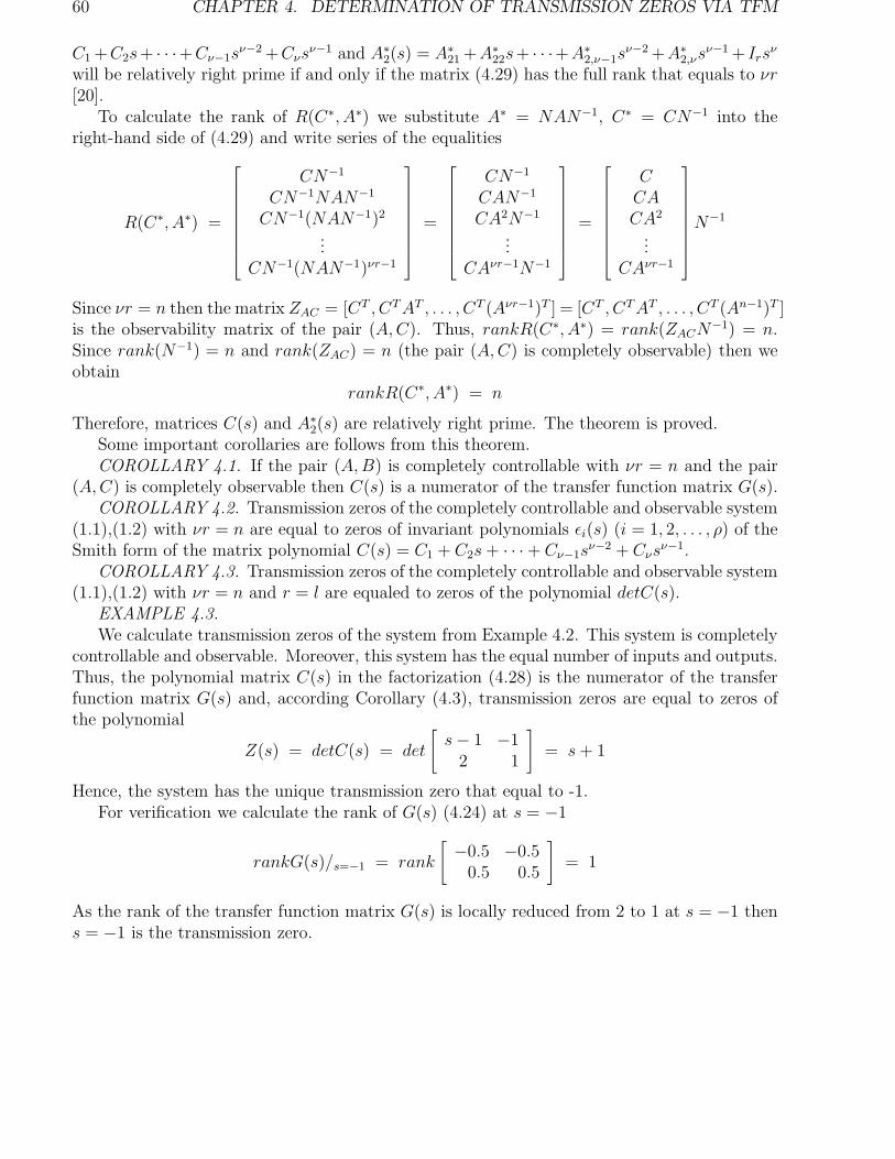
60 CHAPTER 4. DETERMINATION OF TRANSMISSION ZEROS VIA TFM
C1 +C2s+ · · ·+Cν−1sν−2 +Cνs
ν−1 and A∗
2(s) = A∗
21 +A∗
22s+ · · ·+A∗
2,ν−1sν−2 +A∗
2,νsν−1 + Irs
ν
will be relatively right prime if and only if the matrix (4.29) has the full rank that equals to νr[20].
To calculate the rank of R(C∗, A∗) we substitute A∗ = NAN−1, C∗ = CN−1 into theright-hand side of (4.29) and write series of the equalities
R(C∗, A∗) =
CN−1
CN−1NAN−1
CN−1(NAN−1)2
...CN−1(NAN−1)νr−1
=
CN−1
CAN−1
CA2N−1
...CAνr−1N−1
=
CCACA2
...CAνr−1
N−1
Since νr = n then the matrix ZAC = [CT , CTAT , . . . , CT (Aνr−1)T ] = [CT , CTAT , . . . , CT (An−1)T ]is the observability matrix of the pair (A,C). Thus, rankR(C∗, A∗) = rank(ZACN
−1) = n.Since rank(N−1) = n and rank(ZAC) = n (the pair (A,C) is completely observable) then weobtain
rankR(C∗, A∗) = n
Therefore, matrices C(s) and A∗
2(s) are relatively right prime. The theorem is proved.Some important corollaries are follows from this theorem.COROLLARY 4.1. If the pair (A,B) is completely controllable with νr = n and the pair
(A,C) is completely observable then C(s) is a numerator of the transfer function matrix G(s).COROLLARY 4.2. Transmission zeros of the completely controllable and observable system
(1.1),(1.2) with νr = n are equal to zeros of invariant polynomials ǫi(s) (i = 1, 2, . . . , ρ) of theSmith form of the matrix polynomial C(s) = C1 + C2s+ · · · + Cν−1s
ν−2 + Cνsν−1.
COROLLARY 4.3. Transmission zeros of the completely controllable and observable system(1.1),(1.2) with νr = n and r = l are equaled to zeros of the polynomial detC(s).
EXAMPLE 4.3.
We calculate transmission zeros of the system from Example 4.2. This system is completelycontrollable and observable. Moreover, this system has the equal number of inputs and outputs.Thus, the polynomial matrix C(s) in the factorization (4.28) is the numerator of the transferfunction matrix G(s) and, according Corollary (4.3), transmission zeros are equal to zeros ofthe polynomial
Z(s) = detC(s) = det
[
s− 1 −12 1
]
= s+ 1
Hence, the system has the unique transmission zero that equal to -1.For verification we calculate the rank of G(s) (4.24) at s = −1
rankG(s)/s=−1 = rank
[
−0.5 −0.50.5 0.5
]
= 1
As the rank of the transfer function matrix G(s) is locally reduced from 2 to 1 at s = −1 thens = −1 is the transmission zero.

Chapter 5
Zero definition via system matrix
In present chapter we will based on the definition of zeros via (n+ l)× (n+ r) Rosenbrock’ssystem matrix
P (s) =
[
sIn − A −BC O
]
(5.1)
of the normal rank n+min(r, l).
DEFINITION 5.1. A complex frequency s = z at which the normal rank of the matrixP (s) is reduced
rankP (s)/s=z < n+min(r, l) (5.2)
is named as a system zero of system (1.1), (1.2).
First definitions of system zeros have been introduced by prof. Rosenbrock [R2], [R3]. Thedefinition of system zeros as zeros of invariant polynomials of the Smith form of P (s) wasintroduced in 1973 [R2]. More recently these zeros were refereed to as invariant zeros. Thecomplete set of system zeros in terms of special formed minors of P (s) have been introducedin 1974 [R3]. Later we consider these notions more detail. We will consider also other types ofzeros defined in terms of the matrix P (s).
5.1 Complete set of invariant zeros
In Section 3.4 we already have presented the definition of a invariant zero for a system withl ≥ r where r and l are numbers of inputs and outputs respectively. The invariant zero hasbeen defined as a complex frequency that reduces a rank of the matrix P (s). The complete setof invariant zeros consists of the complete set of complex frequencies zi, i = 1, 2, . . . for whichthe rank inequality (5.2) is fulfilled. To find these frequencies we will seek the Smith form S(s)of the matrix P (s). As it was shown in Section 2.5.2, a polynomial (n + l) × (n + r) matrixwith the normal rank n+min(r, l) has the matrix S(s) of the following structure
S(s) = UL(s)P (s)UR(s) =
diag(s1(s), s2(s), . . . , sn+r(s)). . . . . . . . . . . . . . . . . . . . . . . . . . . .
O
, l ≥ r
[diag(s1(s), s2(s), . . . , sn+l(s)), O], l ≤ r
(5.3)
61

62 CHAPTER 5. ZERO DEFINITION VIA SYSTEM MATRIX
where UL(s) and UR(s) are unimodular matrices of dimensions (n+l)×(n+l) and (n+r)×(n+r)respectively, si(s) are invariant polynomials of P (s). We present P (s) as
P (s) = UL(s)−1S(s)UR(s)−1 =
UL(s)−1
diag(s1(s), s2(s), . . . , sn+r(s)). . . . . . . . . . . . . . . . . . . . . . . . . . . .
O
UR(s)−1, l ≥ r
UL(s)−1[diag(s1(s), s2(s), . . . , sn+l(s)), O]UR(s)−1, l ≤ r
(5.4)Since matrices UL(s) and UR(s) are the unimodular ones with constant determinants theninverse matrices UL(s)
−1 and UR(s)−1 have similar properties and a complex s is an invariantzero if and only if it is a zero of any polynomials si(s), i = 1, 2 . . . , n +min(r, l). If l ≥ r thecolumn rank of P (s) is reduced, if l ≤ r the row rank of P (s) is reduced.
Thus, we can define the complete set of invariant zeros as followsDEFINITION 5.1. Zeros of all invariant polynomials si(s), i = 1, . . . , n+min(r, l), taken
all together, form the complete set of invariant zeros.REMARK 5.1. Davison and Wang in 1974 [D4] were defined an invariant zero via the
inequality (5.2) and the ’complete set’ of invariant zeros of a completely controllable and ob-servable system as zeros of the highest order invariant polynomial ( i.e. the polynomial sn+σ(s),σ = min(r, l)). These zeros were named as ’transmission zeros’ [D4] . It is evident that theinvariant zeros of Davison and Wang form a subset of the Rosenbrock’s ones.
REMARK 5.2. It follows from Definition 5.1 and Eqn.(2.37) that the complete set ofinvariant zeros coincides with zeros of the monic largest common divisor ψI(s) of all n+min(r, l)order minors (non identically zero) of the matrix P (s) of the normal rank n + min(r, l). Thepolynomial ψI(s) is
ψI(s) = s1(s)s2(s) · · · , sn+σ(s), σ = min(r, l) (5.5)
This remark may be used for the manual calculating invariant zeros.EXAMPLE 5.1.
We consider the system of the form
x =
1 0 00 −1 00 0 −3
x+
0−1−1
u, y =
[
1 −1 00 2 0
]
x (5.6)
To find the complete set of invariant zeros we construct the matrix
P (s) =
s− 1 0 0 00 s+ 1 0 10 0 s+ 3 11 −1 0 00 2 0 0
(5.7)
and determine minors Pi of the order n + min(r, l) = 3 + 1 = 4 by deleting the row i (i =1, 2, 3, 4, 5). As a result we get
P1 = −2(s+ 3), P2 = 0, P3 = 0, P4 = −2(s− 1)(s+ 3), P5 = (s− 1)(s+ 3)
The monic largest common divisor of non identically zero minors Pi is equal to s+3. Therefore,ψI(s) = s + 3 and the system (5.6) has the only invariant zero z = −3.
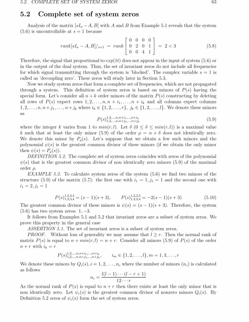
5.2. COMPLETE SET OF SYSTEM ZEROS 63
5.2 Complete set of system zeros
Analysis of the matrix [sIn−A,B] with A and B from Example 5.1 reveals that the system(5.6) is uncontrollable at s = 1 because
rank[sIn − A,B]/s=1 = rank
0 0 0 00 2 0 10 0 4 1
= 2 < 3 (5.8)
Therefore, the signal that proportional to exp(1t) does not appear in the input of system (5.6) orin the output of the dual system. Thus, the set of invariant zeros do not include all frequenciesfor which signal transmitting through the system is ’blocked’. The complex variable s = 1 iscalled as ’decoupling zero’. These zeros will study later in Section 5.3.
Now we study system zeros that form a complete set of frequencies, which are not propagatedthrough a system. This definition of system zeros is based on minors of P (s) having thespecial form. Let’s consider all n+ k order minors of the matrix P (s) constructing by deletingall rows of P (s) expect rows 1, 2, . . . , n, n + i1, . . . , n + ik and all columns expect columns1, 2, . . . , n, n+ j1, . . . , n+ jk where ik ∈ 1, 2, . . . , r, jk ∈ 1, 2, . . . , l. We denote these minorsas
P (s)1,2,...,n,n+i1,...,n+ik1,2,...,n,n+j1,...,n+jk
(5.9)
where the integer k varies from 1 to min(r, l). Let δ (0 ≤ δ ≤ min(r, l)) is a maximal valuek such that at least the only minor (5.9) of the order ρ = n + δ does not identically zero.We denote this minor by Pρ(s). Let’s suppose that we obtain a few such minors and thepolynomial ψ(s) is the greatest common divisor of these minors (if we obtain the only minorthen ψ(s) = Pρ(s)).
DEFINITION 5.2. The complete set of system zeros coincides with zeros of the polynomialψ(s) that is the greatest common divisor of non identically zero minors (5.9) of the maximalorder ρ.
EXAMPLE 5.2. To calculate system zeros of the system (5.6) we find two minors of thestructure (5.9) of the matrix (5.7): the first one with i1 = 1, j1 = 1 and the second one withi1 = 2, j1 = 1
P (s)1,2,3,41,2,3,4 = (s− 1)(s+ 3), P (s)1,2,3,5
1,2,3,4 = −2(s− 1)(s+ 3) (5.10)
The greatest common divisor of these minors is ψ(s) = (s − 1)(s + 3). Therefore, the system(5.6) has two system zeros: 1,−3.
It follows from Examples 5.1 and 5.2 that invariant zeros are a subset of system zeros. Weprove this property in the general case
ASSERTION 5.1. The set of invariant zeros is a subset of system zeros.PROOF. Without loss of generality we may assume that l ≥ r. Then the normal rank of
matrix P (s) is equal to n + min(r, l) = n + r. Consider all minors (5.9) of P (s) of the ordern+ r with ik = r
P (s)1,2,...,n,n+i1,...,n+ik1,2,...,n,n+j1,...,n+jk
, im ∈ 1, 2, . . . , l, m = 1, 3, . . . , r
We denote these minors by Qi(s), i = 1, 2, . . . , nc where the number of minors (nc) is calculatedas follows
nc =l(l − 1) · · · (l − r + 1)
12 · · · rAs the normal rank of P (s) is equal to n + r then there exists at least the only minor that isnon identically zero. Let ψc(s) is the greatest common divisor of nonzero minors Qi(s). ByDefinition 5.2 zeros of ψc(s) form the set of system zeros.

64 CHAPTER 5. ZERO DEFINITION VIA SYSTEM MATRIX
Then we consider all possible minors of the matrix P (s) of order n+r, which are constructedfrom P (s) by deleting superfluously l − r rows from n + l ones. We denote these minors byβi(s), i = 1, 2, . . . , nI where nI is the number of these minors
nI =(n+ l)(n + l − 1) · · · (l − r + 1)
12 · · · (n+ r)
It is clear that nI ≥ nc and the set of Qi(s) is a subset of the set of βi(s). Let ψI(s) is thegreatest common divisor of nonzero βi(s). By Remark 5.2 zeros of the polynomial ψI(s) formthe set of invariant zeros.
Since the set of Qi(s) is the subset of βi(s) then we can write the equality
ψc(s) = ψI(s)ψk(s)
where ψk(s) is non identically zero polynomial. Therefore, the degree of ψI(s) is not greaterthan that of ψc(s). The assertion is proved.
We can illustrate this result using Examples 5.1, 5.2. Indeed system (5.6) has nc = 2 minorsQi(s) (see Example 5.1):
Q1(s) = (s− 1)(s+ 3), Q2(s) = −2(s− 1)(s+ 3)
and nI = 5 minors βi(s) (see Example 5.2):
β1 = −2(s + 3), β1(s) = β1(s) = 0, β4 = −2(s− 1)(s+ 3), β5 = (s− 1)(s+ 3)
The monic greatest common divisor of the minors Qi(s) is ψc(s) = (s− 1)(s+ 3). The monicgreatest common divisor of the nonzero minors βi is ψI(s) = s+ 3. It is evident that the set ofinvariant zeros −3 is the subset of the set of system zeros 1,−3.
ASSERTION 5.2. If l = r and ρ = n + l = n + r then sets of invariant zeros and systemzeros coincide.
The proof follows from the structure of minors Qi(s) and βi(s). These minors are equal tothe only non identically zero minor of order ρ = n + r = n+ l .
Let’s find the minor of form (5.9) when r = l . Using formula for the determinant of a blockmatrix [G1] we get
detP (s) = det
[
sIn −A −BC O
]
= det(sIn−A)det(C(sIn−A)−1B) = det(sIn−A)detG(s)
Thus, the complete set of system zeros of a system with equal number of inputs/outputscoincides with zeros of the polynomial
ψ(s) = det(sIn −A)detG(s) (5.11)
Such definition of system zeros was introduced in [K5].
5.3 Decoupling zeros
In the general case sets of invariant zeros and system zeros are distinguished by presenceof decoupling zeros. We observe this fact in Examples 5.1 and 5.2: the complete set of systemzeros contains the zero z = 1 that does not the invariant zero. This zero coincides with thefrequency at which the system is uncontrollable and the proportional exp(1t) signal does notappear in the input. Such a zero is the decoupling zero. Now we study these zeros.

5.3. DECOUPLING ZEROS 65
Let’s study the structure of the matrix P (s) (5.1). If system (1.1),(1.2) is unobservableor/and uncontrollable then there exists a complex variable s = z at which the normal rank of
the block column
[
sIn − AC
]
or/and the block row [sIn−A,B] is locally reduced. This complex
variable is named as a decoupling zero. These zeros have been introduced by Rosenbrock in 1970[R1]. They associate with complex frequencies (modes, eigenvalues of A), which are decoupledfrom the input/output.
OUTPUT DECOUPLING ZEROS. They appear when several free modal (exponential type)motions of the system state x(t) are decoupled from the output. Let’s consider this situationin detail for the matrix A having n distinct eigenvalues λ1, . . . , λn. Without loss of generalitywe can assume that the forced response is absent ( u(t) = 0). Then using (1.8) we expand thesolution x(t) of linear time-invariant differential equation (1.1) with u(t) = O, to = 0, x(to) =xo 6= O as follows
x(t) =n∑
i=1
wi exp(λit)ξi, ξi = vTi xo
where wi, vTi are right and left eigenvectors of the matrix A, ξi is a nonzero scalar1. We can
express the output of the system as
y(t) = Cx(t) = Cn∑
i=1
wi exp(λit)ξi = Cn∑
i=1
xi(t)
where xi(t) = wiexp(λit)ξi are modal components of the state x(t). If certain modal componentxl(t) = xl = wl exp(λlt)ξl, l ∈ 1, . . . , n is decoupled with the output then the followingcondition is satisfied
Cxl = Cwl exp(λlt)ξl = O (5.12)
As exp(λlt) 6= 0, ξl 6= 0 then it follows from (5.12) that Cwl = O. Adding the last expressionto the following: Awl = wlλl or (λlIn −A)wl = O we obtain
[
λlIn − AC
]
wl = O (5.13)
Considering (5.13) as an linear homogeneous equation in wl we recall that a nontrivial solutionof (5.13) exists if a column rank of the (n+ l)×n block matrix in (5.13) is locally reduced belown. The appropriate value of the complex frequency (λl) is called as the output decoupling zero.
DEFINITION 5.3. Output decoupling zeros are formed by the set of complex variables sat which the normal column rank of the matrix
Po(s) =
[
sIn − AC
]
(5.14)
is reduced.The output decoupling zeros are calculated as zeros of invariant polynomials of Po(s).INPUT DECOUPLING ZEROS. They appear when certain free modal (exponential type)
motions of the state x(t) are decoupled from the input. Considering the dual system we mayshow that there exist an eigenvalue λl and a left eigenvector vl of the matrix A such that thefollowing equalities take place
vTl (λlIn −A) = O, vTl B = O
1We consider nontrivial case when all ξi = vTi xo 6= 0 and the free modal motion of x(t) has all modes.

66 CHAPTER 5. ZERO DEFINITION VIA SYSTEM MATRIX
Uniting these equalities yields
vTl [λlIn − A,B] = O (5.15)
Considering (5.15) as an equation in the vector vTl we conclude that this equation has a non-trivial solution in vTl if the row rank of the n× (n+ r) matrix in (5.15) is locally reduced belown. The appropriate value of the complex frequency λl is called as an input decoupling zero.
DEFINITION 5.4. Input decoupling zeros are formed by the set of complex variables s atwhich the normal row rank of the matrix
Pi(s) = [sIn − A,B] (5.16)
is reduced.The input decoupling zeros are calculated as zeros of invariant polynomials of Pi(s).In Section 2.4.2 we have introduced notions of uncontrollable and unobservable poles, which
coincide with eigenvalues of A reducing the normal rank of matrices [sIn − A,B] and [sIn −AT , CT ]. Now we show that these poles are equal to decoupling zeros.
THEOREM 5.1. Output decoupling zeros and input decoupling zeros of system (1.1), (1.2)coincide with unobservable and uncontrollable poles of this system respectively.
PROOF. Let z is an output decoupling zero. Then the column rank of Po(s) at s = zis locally reduced below n. We need to show that the complex variable z coincides with aneigenvalue of the matrix A. Indeed, if rank Po(s)/s=z < n then there exists a nontrivial vectorf such as Po(z)f = O. Using the structure of Po(s) (5.14) we write the following equations
(zIn −A)f = O (5.17)
Cf = O (5.18)
It follows from (5.17) that z is the eigenvalue of A and f is the corresponding eigenvector. Thuswe immediately obtain from Assertion 2.5 that z is the unobservable pole of (1.1), (1.2).
A similar way may be used for the second part of the theorem.REMARK 5.1. Uncontrollable (unobservable) poles are sometimes refereed as decoupling
poles.NUMBER OF DECOUPLING ZEROS. The following relations can be get from Assertions
2.2, 2.6 and Theorem 5.1:1. The number of input decoupling zeros is equal to the rank deficient of the controllability
matrix YAB = [B,AB, . . . , An−1B].2. The number of output decoupling zeros is equal to the rank deficient of the observability
matrix ZTCA = [CT , ATCT , . . . , (AT )n−1CT ].
INPUT-OUTPUT DECOUPLING ZEROS. They appear when there exist λl, wl and vTlsuch as two equalities (5.13), (5.15) are held simultaneously. Such λl is named as an input-output decoupling zero.
EXAMPLE 5.3.
We consider the system (5.6). If s = 1 then the rank of the matrix
Pi(s) = [sIn − A,B] =
s− 1 0 0 00 s+ 1 0 −10 0 s + 3 −1
is reduced below n = 3
rankPi(s)/s=1 = 2 < 3

5.4. RELATIONSHIP BETWEEN DIFFERENT ZEROS 67
Hence, z = 1 is the input decoupling zero. Let’s find a number of decoupling zeros of thissystem. The rank deficient of the controllable matrix
YAB = [B,AB,A2B] =
0 0 0−1 1 −1−1 3 −9
is equal to 1. So, the system (5.6) has the only input decoupling zero.Then we find the rank deficient of the observability matrix
ZTCA = [CT , ATCT , (AT )2CT ] =
1 0 1 0 0 0−1 2 1 −2 −1 4
0 0 0 0 0 0
It is equal to 1 then the system (5.6) has the only output decoupling zero. To find this zero weconstruct the matrix Po(s)
Po(s) =
[
sIn − AC
]
=
s− 1 0 00 s+ 1 00 0 s+ 31 −1 00 2 0
and discover that the column rank of Po(s) is reduced below n = 3 at s = −3 . Hence, z = −3is the output decoupling zero. Thus, the system (5.6) has the input decoupling zero z = 1 andthe output decoupling zero z = −3.
5.4 Relationship between different zeros
At first we introduce the following notations:
n − a set of system zeros,i − a set of invariant zeros,p − a set of transmission zeros,i.d. − a set of input decoupling zeros,o.d. − a set of output decoupling zeros,i.o.d. − a set of input − output decoupling zeros.
(5.19)
5.4.1 Transmission and invariant zeros
It has been shown that the invariant zeros are associated with reducing a column or rowrank of the matrix P (s).
Let l ≥ r. The normal rank of the (n + l) × (n + r) matrix P (s) is not changed after theright multiplication of P (s) by the nonsingular unimodular (n + r) × (n+ r) matrix
L1(s) =
[
In (sIn − A)−1BO Ir
]
(5.20)
As the determinant of L1(s) does not depend on s then the following rank equalities are satisfied
rankP (s) = rankP (s)L1(s) = rank
[
sIn − A OC C(sIn −A)−1B
]
=

68 CHAPTER 5. ZERO DEFINITION VIA SYSTEM MATRIX
= rank
[
sIn −A OC G(s)
]
(5.21)
Hence, a column rank of P (s) is depended on the rank of G(s): if the rank of G(s) is reducedthen the column rank of P (s) is also reduced.
A similar way may be used for l ≥ r. The normal rank of P (s) is not changed after the leftmultiplication of P (s) by the unimodular (n + l) × (n+ l) matrix
L2(s) =
[
In O−C(sIn −A)−1 Il
]
(5.22)
Thus
rankP (s) = rankL2(s)P (s) = rank
[
sIn −A −BO G(s)
]
(5.23)
and if the rank of G(s) is reduced then the row rank of P (s) is also reduced.We result in that the set of transmission zeros (defined via G(s) ) is the subset of the set
of invariant zeros (defined via P (s)). Using notations (5.19) we summary this result as theinclusion
p ⊆ i (5.24)
The similarly result follows from Assertion 3.1.
5.4.2 Invariant, transmission and decoupling zeros
Let system (1.1), (1.2) with l > r possesses invariant zeros. If a complex variable s = zcoincides with an invariant zero then the column rank of P (s) is reduced. Then there exists anontrivial solution of equation (3.28) with respect to the vector [xTo , u
To ]. Equation (3.28) can
be rewritten for uo = O as
P (z)
[
xoO
]
= O
or in the equivalent form[
zIn − AC
]
xo = O
This expression corresponds to the condition of unobservability and the complex variable zcoincides with an unobservable pole that is equal to an output decoupling zero. Hence, z is aswell the invariant zero as the output decoupling zero. We conclude that if a system has moreoutputs than inputs then several invariant zeros may be output decoupling zeros simultaneously.
The dual situation may take place for a system with l < r, when several zeros are as wellinvariant zeros as input decoupling zeros.
Let’s find conditions when decoupling zeros are simultaneously invariant zeros. Rank equal-ities (5.21),(5.23) demonstrate that invariant zeros, defined via the matrix P (s), contain trans-mission zeros, defined via the matrix G(s), and decoupling zeros, defined either via the matrixPo(s) (l > r) or via the matrix Pi(s) (l < r). Let for l > r the matrix G(s) has a full columnrank. Then if the rank of Po(s) reduces then the rank of P (s) also reduces. Similarly, for l < rif the matrix G(s) has a full row rank then reducing the rank of Pi(s) involves reducing therank of P (s). Therefore, the following assertion is held.
ASSERTION 5.3. Let system (1.1),(1.2) has the matrix G(s) of the full rank. Then if thissystem has more outputs than inputs (l > r) then every output decoupling zero is an invariantzero, i.e.
o.d. ⊂ i (5.25)

5.4. RELATIONSHIP BETWEEN DIFFERENT ZEROS 69
If the system has more inputs than outputs (l < r ) then every input decoupling zero is aninvariant zero, i.e.
i.d. ⊂ i (5.26)
We may show also that the controllability/observability properties are closely connected tothe structure of i. Indeed, if system (1.1),(1.2) with r > l is uncontrollable then the rank ofPi(s) is reduced. Let rankPi(s) = n− q then the system has q uncontrollable poles and the seti differs from the set p by existence of q input decoupling zeros. From (5.24), (5.26) weobtain the following inclusion
i ⊇ p + i.d. (5.27)
Similarly, if system (1.1),(1.2) with l > r is unobservable then the rank of Po(s) is reduced. LetrankPo(s) = n− q, then the system has q unobservable poles and the following inclusion takesplace
i ⊇ p + o.d. (5.28)
If system (1.1),(1.2) is completely controllable and observable then rankPo(s) = rankPi(s) =n for any s. Hence, the normal rank of P (s) is reduced if and only if the normal rank of G(s)is reduced. In this case sets of invariant and transmission zeros coincide
i ≡ p (5.29)
CONCLUSION
In the general case the set i differs from the set p by existence of decoupling zeros.Inclusions (5.27) and (5.28) represent the rough structure of the set i. More exact relationshave been obtained in works [P6], [R3]. In [R3] it has been shown that if r = l then
i = p + o.d. + i.d. − i.o.d.if l > r then
i = p + o.d. + i.d. − some terms of i .d .The calculation of those i.d. that is a part of i is represented in [P6].
If a system is completely controllable and observable then i does not contain decouplingzeros, therefore, the equality (5.29) takes place.
The following example illustrates the situation when the set i does not contain all decou-pling zeros.
EXAMPLE 5.4.
We consider the system (5.6) with the matrix P (s) (5.7). This system has the only invariantzero (-3) that coincides with the output decoupling zero because the column rank of Po(s) isreduced at s = −3
rankPo(s)/s=3 =
−4 0 00 −2 00 0 01 −1 00 2 0
= 2 < 3
Therefore, the zero s = −3 is equal to the output decoupling zero and the invariant zerosimultaneously. Moreover, this system is uncontrollable at s = 1 (see Example 5.3). Hence,s = 1 is the input decoupling zero. But the matrix P (s) has the complete rank at s = 1 becausethere exists the following nonzero minor
P (s)2,3,4,51,2,3,4/s=1 = det
0 2 0 10 0 4 11 −1 0 00 2 0 0
= −8 6= 0

70 CHAPTER 5. ZERO DEFINITION VIA SYSTEM MATRIX
So, the input decoupling zero s = 1 is not the invariant zero. That is why, the set i does notcontain all decoupling zeros.
In the next subsection we show that only the set of system zeros contains all decouplingzeros.
5.4.3 General structure of system zeros
To reveal the structure of the set of system zeros n we will use definitions of system andtransmission zeros from Sections 5.2 and 4.2 respectively. Let the matrix P (s) has the normalrank n+ δ(δ ≤ min(r, l). We consider all nonzero minors of the n+ δ order of the matrix P (s)which are formed according to the relation (5.9). By the block structure of P (s) we can write[G1]
P (s)1,2,...,n,n+i1,...,n+iδ1,2,...,n,n+j1,...,n+jδ
= det(sIn − A)det[Ci1,i2,...,iδ(sIn − A)−1Bj1,j2,...,jδ ]
where i1, . . . , iδ and j1, . . . , jδ are rows and columns of the matrices C and B respectively.Using the relation (4.5) and the last one we can express minors of the transfer function matrixG(s) = C(sIn− a)−1B, which are formed by deleting all rows expect i1, . . . , iδ and all columnsexpect j1, . . . , jδ, as follows
G(s)i1,i2,...,iδj1,j2,...,jδ= det[Ci1,i2,...,iδ(sIn −A)−1Bj1,j2,...,jδ ] =
P (s)1,2,...,n,n+i1,...,n+iδ1,2,...,n,n+j1,...,n+jδ
det(sIn − A)(5.30)
On the other hand minors of G(s) may be represented as
G(s)i1,i2,...,iδj1,j2,...,jδ=
Z(s)i1,i2,...,iδj1,j2,...,jδ
p(s)(5.31)
where p(s) is the least common denominator of minors G(s)i1,i2,...,iδj1,j2,...,jδ. In (5.31) Z(s)i1,i2,...,iδj1,j2,...,jδ
are
polynomials, which are constructed from numerators of G(s)i1,i2,...,iδj1,j2,...,jδsuch a way that the new
minors of G(s) have the polynomial p(s) as the common denominator.By Definitions 2.1, 2,2, zeros of the polynomial p(s), which are poles of TFM G(s), form
a subset of eigenvalues of the matrix A because some eigenvalues of A may coincide withuncontrollable or/and unobservable poles ( decoupling zeros), which are cancelled in the transferfunction matrix G(s). Hence, the following equality takes place
det(sIn −A) = p(s)pd(s) (5.32)
where the polynomial pd(s) has zeros that are unobservable or/and uncontrollable poles ( ordecoupling zeros). Substituting (5.32) into (5.30) and equating the right-hand sides of (5.30)and (5.31) we obtain
P (s)1,2,...,n,n+i1,...,n+iδ1,2,...,n,n+j1,...,n+jδ
= pd(s)Z(s)i1,i2,...,iδj1,j2,...,jδ(5.33)
Thus, by Definitions 5.2, 4.4 and the relation (5.33) we haveASSERTION 5.4. The set of system zeros is formed by sets of transmission and decoupling
zeros.It follows from Assertions 5.1, 5.4 and results of Section 5.4.2 that system zeros contains all
decoupling zeros. This property of system zeros has been illustrated in Example 5.4. The set ofinvariant zeros contains the only zero (−3) that is the output decoupling zero. Two decouplingzeros, namely input decoupling zero (1) and output decoupling zero (−3), are contained in theset of system zeros n = 1,−3 calculated in Example 5.2.
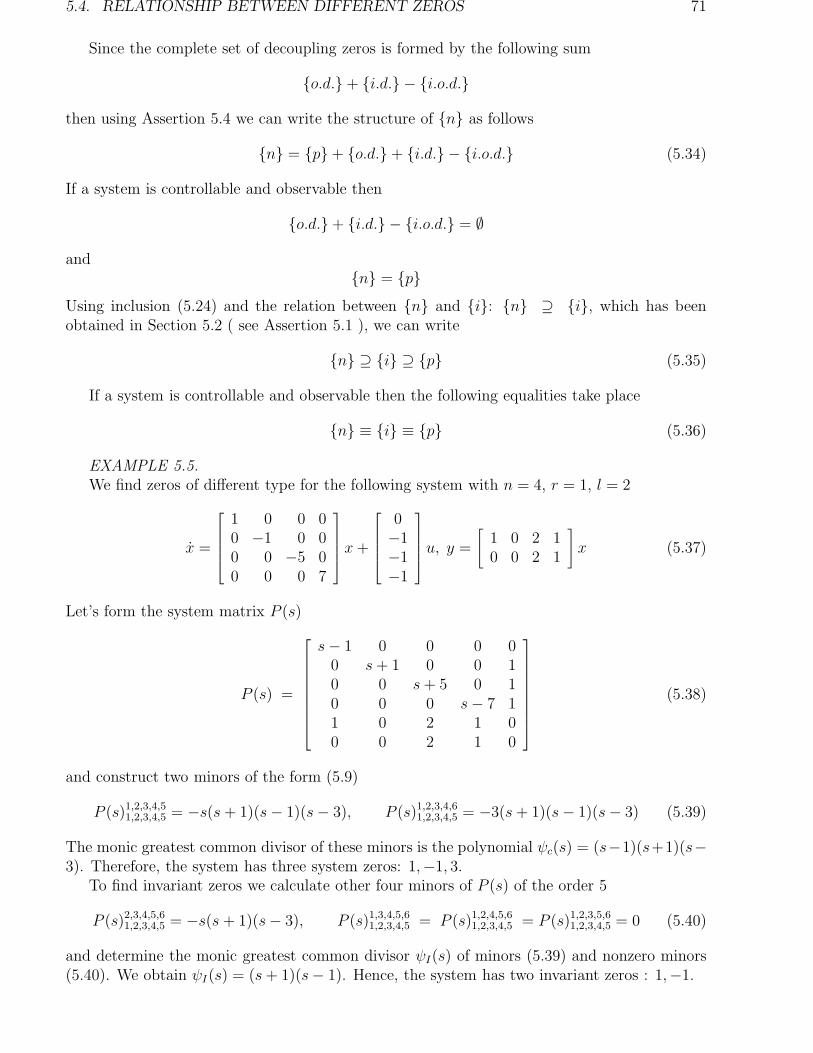
5.4. RELATIONSHIP BETWEEN DIFFERENT ZEROS 71
Since the complete set of decoupling zeros is formed by the following sum
o.d. + i.d. − i.o.d.
then using Assertion 5.4 we can write the structure of n as follows
n = p + o.d. + i.d. − i.o.d. (5.34)
If a system is controllable and observable then
o.d. + i.d. − i.o.d. = ∅
andn = p
Using inclusion (5.24) and the relation between n and i: n ⊇ i, which has beenobtained in Section 5.2 ( see Assertion 5.1 ), we can write
n ⊇ i ⊇ p (5.35)
If a system is controllable and observable then the following equalities take place
n ≡ i ≡ p (5.36)
EXAMPLE 5.5.
We find zeros of different type for the following system with n = 4, r = 1, l = 2
x =
1 0 0 00 −1 0 00 0 −5 00 0 0 7
x+
0−1−1−1
u, y =
[
1 0 2 10 0 2 1
]
x (5.37)
Let’s form the system matrix P (s)
P (s) =
s− 1 0 0 0 00 s+ 1 0 0 10 0 s+ 5 0 10 0 0 s− 7 11 0 2 1 00 0 2 1 0
(5.38)
and construct two minors of the form (5.9)
P (s)1,2,3,4,51,2,3,4,5 = −s(s+ 1)(s− 1)(s− 3), P (s)1,2,3,4,6
1,2,3,4,5 = −3(s+ 1)(s− 1)(s− 3) (5.39)
The monic greatest common divisor of these minors is the polynomial ψc(s) = (s−1)(s+1)(s−3). Therefore, the system has three system zeros: 1,−1, 3.
To find invariant zeros we calculate other four minors of P (s) of the order 5
P (s)2,3,4,5,61,2,3,4,5 = −s(s + 1)(s− 3), P (s)1,3,4,5,6
1,2,3,4,5 = P (s)1,2,4,5,61,2,3,4,5 = P (s)1,2,3,5,6
1,2,3,4,5 = 0 (5.40)
and determine the monic greatest common divisor ψI(s) of minors (5.39) and nonzero minors(5.40). We obtain ψI(s) = (s+ 1)(s− 1). Hence, the system has two invariant zeros : 1,−1.

72 CHAPTER 5. ZERO DEFINITION VIA SYSTEM MATRIX
To find transmission zeros we calculate G(s) = C(sIn −A)−1B
G(s) =
[
1 0 2 10 0 2 1
]
(s− 1)−1 0 0 00 (s+ 1)−1 0 00 0 (s + 5)−1 00 0 0 (s− 7)−1
0−1−1−1
=
=1
(s+ 5)(s− 7)
[
−3(s− 3)−3(s− 3)
]
It is clear that the system has the only transmission zero: 3.From analysis of the matrices
Po(s) =
s− 1 0 0 00 s + 1 0 00 0 s+ 5 00 0 0 s− 71 0 2 10 0 2 1
, Pi(s) =
s− 1 0 0 0 00 s+ 1 0 0 −10 0 s+ 5 0 −10 0 0 s− 7 −1
we find that input and output decoupling zeros are 1 and −1 respectively. So
n = 1,−1, 3i = 1,−1p = 3i.d. = 1o.d. = −1
(5.41)
These sets corroborate the equalities and inclusions, which have been obtained in the presentchapter.
5.5 Summary conclusions from chapters 3 - 5
It has been studied four types of zeros. They are1. TRANSMISSION ZEROS: They are defined via the transfer function matrix G(s). They
are physically associated with transmission-blocking properties of a system, namely, with thetransmission (or blocking) of a steady signal through a system.
2. INVARIANT ZEROS: They are defined via the system matrix P (s). They are physi-cally associated with the zero-output behavior of a system, namely, with the transmission (orblocking) of all parts of a signal ( free and forced ) through a system.
3. DECOUPLING ZEROS: They are defined by matrices Pi(s) = [sIn − A,B], Po(s)T =
[sIn − AT , CT ]. They are associated with existence of system modes that are decoupled withan input or output of a system. These modes are complete uncontrollable or unobservablerespectively.
4. SYSTEM ZEROS : They form the set of zeros including all transmission and decouplingzeros. System zeros are defined via special formed minors of P (s) (5.9).
Chapter 6
Property of zeros
In this chapter we consider main properties, which are inherent to all type of zeros. To studywe will apply elementary block row and column operations on a polynomial matrix. There are
1. interchange any two block rows (columns),2. premultiplication (postmultiplication) any block row (column) by a non singular matrix,3. replacement of a block row (column) by itself plus any other row (column) premultipli-
cated (postmultiplicated) by any polynomial ( or constant) matrix.These elementary block operations correspond to usual elementary operations fulfilled on a
group of rows (columns) and do not change a normal rank of a polynomial matrix.
6.1 Invariance of zeros
The important property of different type zeros is invariance under nonsingular transfor-mations of a state and/or inputs/outputs and also under a state and/or an output feedbackcontrol. We consider this property more detail.
Denoting a set of any type zeros of system (1.1), (1.2) by Ω(A,B,C) we study the followingtransformations.
1. NONSINGULAR TRANSFORMATION OF THE STATE VECTOR : x = Nx where xis a new state vector, N is a nonsingular n×n matrix. Matrices of the transformed system aredefined as follows : A = NAN−1, B = NB, C = CN−1. Zeros of the transformed system arecalculated via the following system matrix
P (s) =
[
sIn − A −BC O
]
=
[
sIn −NAN−1 −NBCN−1 O
]
Applying elementary block operations to P (s) we obtain series of rank equalities
P (s) = rank
[ (
sIn −NAN−1
CN−1
)
N...
−NBO
]
= rank
[
sN −NAC
...−NBO
]
=
rank
N−1(sN −NA) −NB. . . . . . . . . . . . . . . . . . . .
C O
= rank
[
sIn −A −BC O
]
= rankP (s)
Hence, if the rank of P (s) is locally reduced below a normal one at s = z then this propertypossesses the matrix P (s). We obtain the following property.
PROPERTY 6.1. Zeros are invariant under the nonsingular transformation of state variables
Ω(A,B,C) = Ω(NAN−1, NB,CN−1) (6.1)
73

74 CHAPTER 6. PROPERTY OF ZEROS
2. NONSINGULAR TRANSFORMATION OF THE INPUT VECTOR: u = Mu where uis a new input, M is a nonsingular r× r matrix. A new input matrix is defined as B = BM−1.Calculating a rank of the transformed matrix P (s) we obtain
rankP (s) = rank
[
sIn − A −BM−1
C O
]
= rank
[
sIn − AC
...
(
−BM−1
O
)
M
]
= rankP (s)
Thus, the following property takes placePROPERTY 6.2. Zeros are invariant under the nonsingular transformation of input vari-
ablesΩ(A,B,C) = Ω(A,BM−1, C) (6.2)
3. NONSINGULAR TRANSFORMATION OF THE OUTPUT VECTOR: y = Ty wherey is a new output, T is a nonsingular l× l matrix. A new output matrix is defined as C = TC.Applying the following elementary block operations we transform the matrix P (s) as
rankP (s) = rank
[
sIn −A −BTC O
]
= rank
sIn − A −B. . . . . . . . . . . . . . .T−1(TC, O)
= rankP (s)
and formulate the following property.PROPERTY 6.3. Zeros are invariant under the nonsingular transformation of output vari-
ablesΩ(A,B,C) = Ω(A,B, TC) (6.3)
We unite Properties 6.1-6.3 as follows
Ω(A,B,C) = Ω(NAN−1, NBM−1, TCN−1) (6.4)
4. STATE AND OUTPUT PROPORTIONAL FEEDBACK. Let us inset a linear propor-tional state feedback to system (1.1),(1.2)
u = Kx+ v (6.5)
where v = v(t) is a new external reference input. The closed-loop system is described by theequation
x = (A+BC)x+Bv (6.6)
with the output (1.2). To find a rank of the system matrix Pc(s) of Eqns. (6.6), (1.2) we usethe following elementary block operations
rankPc(s) = rank
[
sIn − (A+BK)C
...−BO
]
=
= rank
[ (
sIn − (A+BK)C
)
−(
−B0
)
K...
−BO
]
= rankP (s) (6.7)
We have the similar result if use a linear proportional output feedback u = Ky+ v = KCx+ vwhen the matrix K is changed by KC in (6.7).
Therefore, we deduce the following property.PROPERTY 6.4. Zeros are invariant under the proportional state and output feedback
Ω(A,B,C) = Ω(A +BK,B,C) = Ω(A +BKC,B,C) (6.8)
Uniting (6.4) and (6.8) we obtain the general formula of zero invariance
Ω(A,B,C) = Ω(N(A +BKC)N−1, NBM−1, TCN−1) (6.9)

6.2. SQUARING DOWN OPERATION 75
6.2 Squaring down operation
Let system (1.1), (1.2) has more outputs than inputs (l > r). To get a new system withequal number of inputs and outputs we combine output variables to replace the l vector y = Cxby a new output r vector
y = Ly = LCx (6.10)
where L is an r × l matrix of a full rank. The mentioned operation is refereed as ’squaringdown’ [M1].
If we add extra input variables to form a new input l vector u by the rule
u = Du (6.11)
where D is an r× l matrix then this operation is refereed as ’squaring up’ [M1]. Later we studyin detail the squaring down operation because its practical applicability.
At first we consider the following important property of the squaring down operation.ASSERTION 6.1. A zero set of system (1.1),(1.2) with l > r is a subset of zeros of the
squared down system (1.1),(6.10)
Ω(A,B,C) ⊆ Ω(A,B, LC) (6.12)
but vice versa of the relation (6.12) is not held.PROOF. For definiteness we assume that the r × l matrix L of the rank r has the form
L = [L1, L2] (6.13)
where L1 is a nonsingular r× r matrix. At first we consider a particular case when L = [Ir, O].The system matrix P (s) of the squared down system has the following structure
P (s) =
[
sIn − A −BC1 O
]
(6.14)
where C1 is the r × n block row of the l × n output matrix C =
[
C1
C2
]
. Zeros of the squared
down system coincides with zeros of the greatest common divisor of minors of P (s) of a maximalorder.
Then writing the system matrix for Eqns. (1.1), (1.2) with CT = [CT1 , C
T2 ]
P (s) =
sIn − A −BC1 OC2 O
(6.15)
we can see that zeros of system (1.1),(1.2) coincides with zeros of a greatest common divisorof a maximal order minors of the (n + l) × (n + r) matrix (6.15). It is evident that the setof minors of P (s) includes the set of minors of P for l > r. Hence, we have been proved theassertion for L = [Ir, O], i.e.
Ω(A,B,C) ⊆ Ω(A,B, [Ir, O]C) (6.16)
Now we consider the general case of L (6.13) and define a nonsingular l × l matrix
T =
[
L−11 −L−1
1 L2
O Il−r
]

76 CHAPTER 6. PROPERTY OF ZEROS
Such the matrix exists because rankL1 = r. It is clear that
LT = [Ir, O] (6.17)
From (6.16) and (6.17) we obtain the following inclusions for any l×n matrix C∗ of a full rank
Ω(A,B,C∗) ⊆ Ω(A,B, [Ir, O]C∗) ⊆ Ω(A,B, LTC∗)
orΩ(A,B,C∗) ⊆ Ω(A,B, LTC∗) (6.18)
On the other hand, since T is the nonsingular l × l matrix, then the set Ω(A,B,C∗) becomesby Property 6.3
Ω(A,B,C∗) = Ω(A,B, TC∗) (6.19)
Substituting the right-hand side of (6.19) into the left-hand side of (6.18) we get
Ω(A,B, TC∗) ⊆ Ω(A,B, LTC∗) (6.20)
Then defining C∗ = T−1C we present (6.20) as
Ω(A,B, TT−1C) ⊆ Ω(A,B, LTT−1C)
orΩ(A,B,C) ⊆ Ω(A,B, LC)
The inclusion obtained completes the proof.Let system (1.1),(1.2) has r > l. We form a new input l vector u by rule (6.11). This is
the squared down operation for inputs because the number of inputs are decreased from r to l.Similarly to Assertion 6.1 we can prove
ASSERTION 6.2. Any set of zeros of system (1.1), (1.2) with r > l is a subset of zeros ofthe squared down system (1.1),(1.2),(6.11)
Ω(A,B,C) ⊆ Ω(A,BD,C) (6.21)
but vice versa does not true.EXAMPLE 6.1.
To illustrate the result we consider the following system with n = 3, r = 1, l = 2
x =
1 0 00 −1 −11 0 −1
x+
−100
u, y =
[
1 0 00 2 0
]
x (6.22)
At first we construct the system matrix
P (s) =
s− 1 0 0 10 s+ 1 1 0−1 0 s+ 1 01 0 0 00 2 0 0
(6.23)
and calculate two minors of the order 4 :
P (s)1,2,3,41,2,3,4 = (s+ 1)2, P (s)1,2,3,5
1,2,3,4 = 2 (6.24)

6.3. ZEROS OF CASCADE SYSTEM 77
The monic greatest common divisor of these minors is equal to ψc(s) = 1. Hence, the systemhas no zeros. Let’s combine output variables to form the new scalar output y
y = [ 1 1 ]y = [ 1 1 ]
[
y1
y2
]
= y1 + y2 (6.25)
In this case the squared down compensator L is equal to [ 1 1 ] and the new output matrixbecomes
C = LC = [ 1 1 ]
[
1 0 00 2 0
]
= [ 1 2 0 ]
We build the system matrix of the new system
P (s) =
s− 1 0 0 10 s+ 1 1 0−1 0 s+ 1 01 2 0 0
and calculate the only minor of P (s) that is ψc(s) = −(s2 + 2s − 1). Zeros of ψc(s) arez1 = −1 +
√2, z2 = −1 −
√2. Thus, we see that the squaring down operation introduces
new zeros into the system. This property must be taken into account when squared downcompensators L and/or D are used. For example, such a problem inevitably appears in acascade connection of systems.
6.3 Zeros of cascade system
Let us consider two systems S1 and S2
S1 : x1 = A1x1 +B1u, y1 = C1x1
S2 : x2 = A2x2 +B2u, y2 = C2x2
where a number of outputs of the first system differs from a number of inputs of the secondone. In above equations vectors x1, x2, u1, u2, y1, y2 have dimensions n1 × 1, n2 × 1, r1 × 1,r2 × 1, l1 × 1, l2 × 1 respectively.
The cascade connection of S1 and S2 is as follows: we insert a linear combination of variablesof the output y1 to the input u2 , i.e. we use the connection
u2 = Gy1 (6.26)
with an r2 × l1 compensator G .Let every Si, i = 1, 2 has a zero set Ωi, i = 1, 2. To find a zero set of the augmented system
we substitute the relation (6.26) in S2 and write the augmented system[
x1
x2
]
=
[
A1 OB2GC1 A2
] [
x1
x2
]
+
[
B1
O
]
u1,
y =[
O C2
][
x1
x2
]
(6.27)
Let us find the rank of the system matrix Ps1+s2 of system (6.27) by using the following rankequalities
rankPs1+s2 = rank
sIn1−A1 O −B1
B2GC1 sIn2− A2 O
O C2 O
=
78 CHAPTER 6. PROPERTY OF ZEROS
= rank
In1O O
O sIn2− A2 −B2
O C2 O
sIn1−A1 O −B1
O In2O
GC1 O O
(6.28)
On the other hand
rankPs1+s2 = rank
In1O O
O sIn2− A2 −B2G
O C2 O
sIn1−A1 O −B1
O In2O
C1 O O
(6.29)
We limit our study by systems S1 and S2 having such a number of inputs and outputs thatprovides the product of square matrices in the right-hand sides of (6.28), (6.29). Hence, wehave two cases:
1. l1 ≥ r1 = r2 = l2. Using Eqn.(6.28) we need to evaluate
detPs1+s2 = det
In1O O
O sIn2−A2 −B2
O C2 O
det
sIn1− A1 O −B1
O In2O
GC1 O O
At first we decrease the dimensions of block matrices by expanding unity blocks and representdetPs1+s2 as
detPs1+s2 = det
[
sIn2− A2 −B2
C2 O
]
det
[
sIn1−A1 −B1
GC1 O
]
(6.30)
It is evident that a rank of the matrix Ps1+s2 is reduced if and only if ranks of the system matrixof S2 or the following squared down system
S∗
1 : x1 = A1x1 +B1u1, y1 = GC1x1 (6.31)
are reduced.Let’s denote zero sets of systems (6.27) and (6.31) by Ωs1+s2 and Ω∗
s1respectively. It follows
from the equality (6.30)
Ωs1+s2 = Ωs2 ∪ Ω∗
s1(6.32)
2. r2 ≥ l2 = l1 = r1. Using similar way we obtain from (6.29) the following equalities
detPs1+s2 = det
In1O O
O sIn2− A2 −B2G
O C2 O
det
sIn1− A1 O −B1
O In2O
C1 O O
=
= det
[
sIn2−A2 −B2GC2 O
]
det
[
sIn1−A1 −B1
C1 O
]
So, a rank of the matrix Ps1+s2 is reduced if and only if ranks of the system matrix of S1 or thesquared down system
S∗
2 : x2 = A2x2 +B2Gu2, y2 = C2x2 (6.33)
are reduced. Denoting a zero set of system (6.33) by Ω∗
s2we can write the following equality
Ωs1+s2 = Ωs1 ∪ Ω∗
s2 (6.34)
Now we analyze relations (6.32),(6.34). In the first case the system S∗
1 is obtained from S1
by squaring down its outputs. In the second case the system S∗
2 is obtained from S2 by squaring

6.3. ZEROS OF CASCADE SYSTEM 79
down its inputs. Above we have shown that the squaring down operation introduces new zerosinto a system. Denoting the set of introducing zeros by Ωsq we represent sets Ω∗
s1and Ω∗
s2as
Ω∗
si= Ωsi
∪ Ωsq, i = 1, 2 (6.35)
and rewrite (6.32) or (6.34) using (6.35) as the only sum
Ωs1+s2 = Ωs1 ∪ Ωs2 ∪ Ωsq (6.36)
So, it has been shown: The cascade connection of systems with different numbers of inputs andoutputs may introduce additional zeros into an augmented system. Hence, it is necessary tochoose the matrix G to shift these zeros to the left-hand side of the complex plan.
Let’s consider the important particular case when systems S1 and S2 have same numbersof inputs and outputs : r1 = l1 = r2 = l2. In this case G is a square nonsingular matrix whichtransforms outputs of S1 or inputs S2. According Properties 6.2, 6.3 we have
Ω∗
s1 = Ωs1 , Ω∗
s2 = Ωs2 , Ωsq = ∅
and the zero set of the augmented system is
Ωs1+s2 = Ωs1 ∪ Ωs2 (6.37)
The next assertion is the direct corollary of the equality (6.37).ASSERTION 6.3. The set of zeros of the cascade connection of systems S1,. . . ,Sk having
equal numbers of inputs and outputs is defined as
Ωs1+s2+···+sk= Ωs1 ∪ Ωs2 ∪ · · · ∪ Ωsk
EXAMPLE 6.2.Let us consider two systems
x1 =
[
1 00 2
]
x1 +
[
11
]
u1, y1 = x1 (6.38)
x2 =
[
2 01 1
]
x2 +
[
10
]
u2, y2 =[
1 2]
x2 (6.39)
We insert a linear combination of variables of y1 to the input u2 of the second system, i.e. weuse the connection :
u2 = Gy1 (6.40)
Substituting (6.40) into (6.39) and using (6.38) we can write the following augmented system
[
x1
x2
]
=
[
A1 OB2GC1 A2
] [
x1
x2
]
+
[
B1
O
]
u1,
y =[
O C2
][
x1
x2
]
where
A1 =
[
1 00 2
]
, A2 =
[
2 01 1
]
, B1 =
[
11
]
, C1 =
[
1 00 1
]
, B2 =
[
10
]
, C2 =[
1 2]
Zeros of systems (6.38), (6.39) are respectively Ωs1 = ∅, Ωs2 = −1.

80 CHAPTER 6. PROPERTY OF ZEROS
Let’s assignG = [ 1 1 ]
and find zeros of the squared down system S∗
1 : x1 = A1x1 +B1u1, y1 = Gy1 = GC1x1.We obtain Ω∗
s1 = 1.5. Therefore, the squared down operation introduces the only zero(z = 1.5), i.e. Ωsq = 1.5. Using formula (6.36) we can determine the set of zeros of theoverall cascade connection: Ωs1+s2 = ∅ ∪ −1 ∪ 1.5 = −1, 1.5.
For checking we calculate zeros of the augmented system with G = [ 1 1 ]. The systemmatrix Ps1+s2 of the cascade connection system is
Ps1+s2 =
s− 1 0 0 0 −10 s− 2 0 0 −11 1 s− 2 0 00 0 −1 s− 1 00 0 1 2 0
Determining detPs1+s2 = −(2s− 3)(s+ 1) we obtain Ωs1+s2 = 1.5,−1.
6.4 Dynamic output feedback
Now we study the effect of a dynamic regulator (dynamic output feedback) on system zeros.To this point we insert the following linear dynamic output feedback
z = Fz +Qy (6.41)
u = v −K1z (6.42)
into system (1.1), (1.2). Here z the p× 1 state vector of the dynamic regulator, v is the r × 1reference input vector and constant matrices F , Q, K1 have the corresponding sizes.
Substituting (6.41), (6.42) into (1.1), (1.2) and denoting the new state vector as [xT , zT ]gives the following closed-loop augmented system
[
xz
]
=
[
A −BK1
QC F
] [
xz
]
+
[
BO
]
v,
y =[
C O][
xz
]
(6.43)
with the input r vector v and the output l vector y. To find zeros of this system we need toanalyze its the system matrix
P (s) =
sIn+p −[
A −BK1
QC F
]
... −[
BO
]
. . . . . . . . . . . . . . . . . . . . . . . . . . . . . . . .[
C O] ... O
=
sIn − A −BK1 −B−QC sIp − F OC O O
Let’s carry out several elementary block operations on the matrix P (s): We fulfill left and rightmultiplications of P (s) by unimodular matrices and then interchange the second and the thirdblock rows and the appropriate columns. We result in following rank equalities
rankP (s) = rank
In O OO Ip OO O Il
sIn − A −BK1 −B−QC sIp − F OC O O
In O OO Ip OO K1 Il
=

6.4. DYNAMIC OUTPUT FEEDBACK 81
= rank
sIn − A O −BO sIp − F OC O O
=
sIn − A −B ... O
C O... O
. . . . . . . . . . . . . . . . .
O O... sIp − F
(6.44)
Hence, the rank of P (s) is locally reduced at s = s∗ if and only if s∗ coincides with a zero ofsystem (1.1), (1.2) or with an eigenvalue of the matrix F .
The similar result may be obtain for the feedback regulator of the general structure
z = Fz +Qy,
u = v −K1z −K2y = v −K1z −K2Cx (6.45)
where K2 is a constant r × l matrix. The system matrix for system (1.1),(1.2) with regulator(6.45) is
P (s) =
sIn − (A−BK2C) −BK1 −B−QC sIp − F OC O O
Executing elementary block operations on P (s) we can show that
rankP (s) = rank
sIn − (A− BK2C) −B ... O
C O... O
. . . . . . . . . . . . . . . . . . . . . . . . . . . .
O O... sIp − F
= rank
sIn − A −B ... O
C O... O
. . . . . . . . . . . . . . . . .
O O... sIp − F
(6.46)Thus, it follows from (6.44) and (6.46)
ASSERTION 6.4. The set of zeros of the augmented system with the dynamic regulator(6.41), (6.42) or (6.45) consists of all zeros of system (1.1),(1.2) and all eigenvalues of the matrixdynamics F of the regulator.
Therefore, we conclude that a dynamic feedback introduces additional zeros in any system.This result generalizes the similar property of the classic single-input/ single-output system,namely, zeros of any closed-loop transfer function include zeros of an open-loop transfer functionand poles of a compensator transfer function.
Let us consider the important case of a dynamic regulator, namely, the proportional-integral(PI) regulator
z = y, u = v −K1z − K2x (6.47)
PI-regulator (6.47) is the particular case of the dynamic regulator (6.45) with p = l, F =O, Q = Il, K2C = K2. We have from Assertion 6.4
COROLLARY 6.1. Any PI-regulator of the order l introduces l zeros in origin.EXAMPLE 6.3.
To study the affect of the dynamic feedback we consider the following simple system
x =
[
−1 01 2
]
x+
[
10
]
u, y =[
1 1]
x (6.48)
and the dynamic regulator of the structure (41),(42)
z = 2z + y = 2z + [ 1 1 ]x (6.49)

82 CHAPTER 6. PROPERTY OF ZEROS
u = v − z − y = v − z − [ 1 1 ]x (6.50)
Here p = 1, F = 2, Q = 1, K1 = 1, K2 = 1. Substituting (6.50) in (6.48)
x =
[
−1 01 2
]
x+
[
10
]
[ 1 1 ]x−[
10
]
z +
[
10
]
v =
[
−2 −11 2
]
x−[
10
]
z +
[
10
]
v
and uniting this equation with (6.49) we obtain the augmented system
[
xz
]
=
−2 −1 −11 2 01 1 2
[
xz
]
+
100
v,
y =[
1 1 0][
xz
]
(6.51)
To find zeros of (6.51) we construct
P (s) =
s+ 2 1 1 −1−1 s− 2 0 0−1 −1 s− 2 01 1 0 0
and find the zero polynomial ψ(s) = (s − 2)(s − 1). Therefore, the closed-loop system (6.51)has two zeros : s1 = 2, s2 = 1.
For testing we calculate zeros of system (6.48) and obtain the only zero (s1 = 1). Since oneeigenvalue of the matrix dynamics of (6.49) is equal to 2 then we have obtained the corroborationof Assertion 6.4.
6.5 Transmission zeros and high output feedback
Let a linear negative proportional output feedback
u = −Ky (6.52)
is applied into completely controllable and observable system (1.1),(1.2) having equal numbersof inputs and outputs (r = l).
We will investigate asymptotic behavior of eigenvalues of the dynamics matrix A − BKCof the closed-loop system when elements of the gain matrix K unlimited increase. For thispurpose we represent the matrix K as
K = kK
where K is a constant r× r matrix of a full rank with bounded elements and k is a scalar valuethat increases to infinity.
For φ(s) = det(sIn − A) and φc(s) = det(sIn − (A− BKC)), characteristic polynomials ofthe open-loop and closed-loop systems respectively, we prove the following assertion.
ASSERTION 6.5. [H1].φc(s)
φ(s)= det(Ir +KG(s)) (6.53)
PROOF. At first we express φc(s) via φ(s)
φc(s) = det(sIn − (A− BKC)) = det(sIn − A)(In + (sIn −A)−1BKC) =
6.5. TRANSMISSION ZEROS AND HIGH OUTPUT FEEDBACK 83
= det(sIn − A)det(In + (sIn − A)−1BKC) = φ(s)det(In + (sIn − A)−1BKC)
Denoting N = (sIn−A)−1B, M = KC and using the equality from [K5, lemma 1.1]: det(In +NM) = det(Ir + MN) where matrices M , N of dimensions r × n and n × r respectively, wetransform the expression in the right-hand side of the last equality as
φc(s) = φ(s)det(sIn − A)−1BKC) = φ(s)det(Ir +KC(sIn −A)−1B)
This proves the assertion.Rewriting (6.53) with K = kK (k 6= 0)
φc(s) = φ(s)det(Ir + kKG(s)) = φ(s)detk( 1
kIr + KG(s))
and taking out k from the determinant
φc(s) = φ(s)krdet(1
kIr + KG(s)) (6.54)
we analyze the relation (6.54) as k → ∞
limk→∞
φc(s) = φ(s)krdet(KG(s)) = krφ(s)detKdetG(s) (6.55)
As it has been shown in Section 5.2 the following polynomial
φ(s)detG(s) = det(sIn − A)det(C(sIn −A)−1B)
is the zero polynomial of system (1.1),(1.2) with r = l. Denoting ψ(s) = φ(s)detG(s), d =detK we can rewrite (6.55) as follows
limk→∞
φc(s) = dkrψ(s) (6.56)
Hence, as k → ∞ n− r eigenvalues of the matrix A−BkKC will asymptotically achieve zerolocations while the remainder r eigenvalues will tend to infinity.
REMARK 6.1. The result obtained extends the known classic root-locus method to multi-variable systems.

84 CHAPTER 6. PROPERTY OF ZEROS
Chapter 7
System zeros and matrix polynomial
In this chapter we will study a definition of system zeros via an l × r matrix polynomial ofa degree ν − 1 where ν is the controllability index of the pair (A,B). Above in Section 4.3 wehave already introduced the similar definition of transmission zeros for a system with n = rνwhere n, r are an order and number of inputs (see Corollary 4.2). Now we consider the generalcase n 6= rν. This definition was introduced by Smagina [S4] in 1981 and will use for studyimportant properties of zeros such as a maximal number of zeros and its relations with theMarkov parameter matrices CB,CAB, . . ..
7.1 Zero definition via matrix polynomial
Using the nonsingular transformation of state and input variables
z = Nx, v = M−1u
we reduce completely controllable system (1.1), (1.2) to Yokoyama’s canonical form (1.61)
z = Fz +Gv, y = CN−1z (7.1)
where
F = NAN−1 =
F1
. . . . . . . . . . . . . . . .Fν1, Fν2, . . . , Fνν
, G = NBM =
[
OGν
]
(7.2)
The structure of nonzero blocks F1 (1.62), Gν (1.65) of dimensions (n − r) × n and r × rrespectively are depended on integers ν and l1, l2, . . . , lν (1.59), (1.60).
As it has been shown in Section 6.1 system zeros are invariant under state and inputnonsingular transformations. Therefore, system zeros of (1.1),(1.2) are equal to system zerosof system (7.1) and defined via the following system matrix
P (s) =
[
sIn − F −GCN−1 O
]
(7.3)
Let’s partition the matrix CN−1
CN−1 = [ C1, C2, . . . , Cν ] (7.4)
where Ci are l × li blocks and construct the following l × r matrix polynomial 1 of the degreeν − 1
C(s) = [O,C1] + [O,C2]s+ · · · + [O,Cν−1]sν−2 + Cνs
ν−1 (7.5)1The definition of a matrix polynomial has been introduced in Sec.1.2.1
85

86 CHAPTER 7. SYSTEM ZEROS AND MATRIX POLYNOMIAL
Now we show that system zeros of controllable system (1.1), (1.2) are defined in terms of thematrix polynomial (7.5).
At first we consider the particular case r = l.THEOREM 7.1. System zeros of controllable system (1.1),(1.2) with a similar number of
inputs and outputs are defined as zeros of the following polynomial
ψ(s) = sn−rνdetC(s) (7.6)
where integer ν is the controllability index of the pair (A,B) (see (1.45)).PROOF. In this case the system matrix (7.3) has the only minor of the maximal order
n+ r
P (s)1,2,...,n,n+1,...,n+r1,2,...,n,n+1,...,n+r = det
[
sIn − F −GCN−1 O
]
(7.7)
Zeros of the minor (7.7) (that is a polynomial in s) coincide with system zeros (see Definition5.2). To find the determinant in (7.7) we partition the matrix sIn−F with F from (1.62) intofour blocks
sIn − F =
sIn−r − F11... −F12
. . . . . . . . . . . . . . . . . . . . . . . . . . . . . . . .
−Fν1,−Fν2, . . . ,−Fν,ν−1... sIr − Fνν
(7.8)
where Fνi are r× li submatrices (i = 1, 2, . . . , ν), matrices sIn−r−F11 and F12 have dimensions(n− r)× (n− r) and (n− r)× r respectively. Substituting (7.8) and (7.4) into the right-handside of (7.7) and using the structure of G (1.64) we can present detP (s) as
detP (s) = det
sIn−r − F11... −F12
... O
−Fν1,−Fν2, . . . ,−Fν,ν−1... sIr − Fνν
... −Gν
C1, C2, . . . , Cν−1... Cν
... O
=
det
sIn−r − F11... −F12
... O
C1, C2, . . . , Cν−1... Cν
... O
Fν1, Fν2, . . . , Fν,ν−1... −sIr + Fνν
... Gν
= det
sIn−r − F11... −F12
. . . . . . . . . . . . . . . . . . . .
C1, C2, . . . , Cν−1... Cν
det(Gν)
(7.9)To calculate the determinant of the block matrix in the right hand-side of (7.9) we use theformula from [G1]( assuming s 6= 0)
det
sIn−r − F11... −F12
. . . . . . . . . . . . . . . . . . . .
C1, C2, . . . , Cν−1... Cν
det(Gν) =
det(sIn−r − F11)(det(Cν + [C1, C2, . . . , Cν−1](sIn−r − F11)−1F12) (7.10)
Since structures of matrices F11 and F12 coincide with ones of P11 and P12 respectively (see(1.27) with p = ν) then according results of Section 1.2.1 we find
det(sIn−r − F11) = sl1+l2+···+lν−1 = sn−r (7.11)
(sIn−r − F11)−1F12 =
s1−ν [O, Il1]s2−ν [O, Il2]
...s−1[O, Ilν−1
]
(7.12)

7.1. ZERO DEFINITION VIA MATRIX POLYNOMIAL 87
where [O, Ili] are li × r matrices. Substituting (7.11) and (7.12) into (7.10)
det
sIn−r − F11... −F12
. . . . . . . . . . . . . . . . . . . .
C1, C2, . . . , Cν−1... Cν
= sn−rdet(Cν+[C1, C2, . . . , Cν−1]
[O, Il1]s[O, Il2]
...sν−2[O, Ilν−1
]
s1−ν) =
= sn−rsr−rνdet[C1, C2, . . . , Cν]
[O, Il1]s[O, Il2]
...sν−2[O, Ilν−1
]sν−1Ir
) = sn−rνdet([O,C1]+[O,C2]s+· · ·+Cνsν−1) =
= sn−rνdetC(s) (7.13)
and the right-hand side of (7.13) into (7.9) we get the final expression for detP (s)
detP (s) = sn−rνdetC(s)det(Gν) (7.14)
Since the r × r matrix Gν is nonsingular one then zeros of detP (s) coincide with zeros of thepolynomial ψ(s) = sn−rνdetC(s). This proves the theorem.
REMARK 7.1. The formula (7.6) is also true for s = 0. Indeed, calculating the determinantof the matrix P (s) (7.9) at s = 0 we obtain
detP (0) = det
−F11... −F12
. . . . . . . . . . . . . . . . . . . .
C1, C2, . . . , Cν−1... Cν
det(Gν) = (−1)n−rdet[C1, C21, . . . , Cν1]det(Gν)
where Ci1 are r× (li− li−1) submatrices of matrices Ci = [Ci1, Ci2], i = 2, 3, . . . , ν. On the otherhand using the structure of (7.5) we can calculate
sn−rνdetC(s)/s=0 =
sn−rνdet[O,C1] + [O,C2diag(Il2s)] + [O,C3diag(Il3s2)] + · · ·+ [O,Cν−1diag(Ilν−1s
ν−2)]+
+Cνdiag(Irsν−1)/s=0 = det[O,C1] + [O, (C21, C22)diag(Il2−l1 , Il1s]+
+[O, (C31, C32, C33)diag(Il3−l2, Il2−l1s, Il1s2] + · · ·+
+[Cν1, Cν2, · · · , Cνν ]diag(Ir−lν−1, Ilν−1−lν−2
s, . . . Il1sν−1)/s=0 =
= det(Cν1, Cν2, . . . , C21, C1)
Thus, detP (s)/s=0 = 0 if and only if sn−rνdetC(s)/s=0 = 0.REMARK 7.2. Consider the particular case when system (1.1),(1.2) has n = rν, l1 =
l2 = · · · = lν = r. Such system is reduced to Asseo’s canonical form and the matrix CN−1 ispartitioned into (l×r) blocks Ci. As a result the matrix polynomial (7.5) becomes the simpleststructure
C(s) = C1 + C2s + · · ·+ Cνsν−1 (7.15)
The zero polynomial is defined asψ(s) = detC(s) (7.16)
EXAMPLE 7.1.
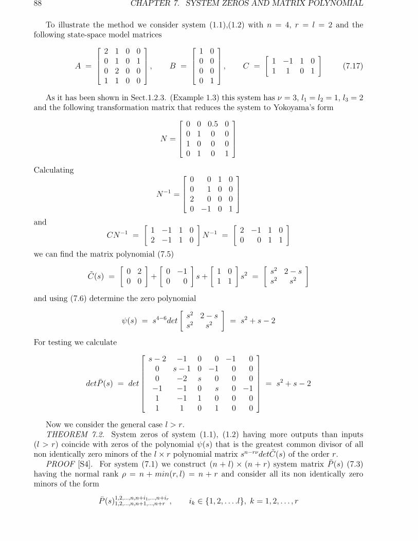
88 CHAPTER 7. SYSTEM ZEROS AND MATRIX POLYNOMIAL
To illustrate the method we consider system (1.1),(1.2) with n = 4, r = l = 2 and thefollowing state-space model matrices
A =
2 1 0 00 1 0 10 2 0 01 1 0 0
, B =
1 00 00 00 1
, C =
[
1 −1 1 01 1 0 1
]
(7.17)
As it has been shown in Sect.1.2.3. (Example 1.3) this system has ν = 3, l1 = l2 = 1, l3 = 2and the following transformation matrix that reduces the system to Yokoyama’s form
N =
0 0 0.5 00 1 0 01 0 0 00 1 0 1
Calculating
N−1 =
0 0 1 00 1 0 02 0 0 00 −1 0 1
and
CN−1 =
[
1 −1 1 02 −1 1 0
]
N−1 =
[
2 −1 1 00 0 1 1
]
we can find the matrix polynomial (7.5)
C(s) =
[
0 20 0
]
+
[
0 −10 0
]
s+
[
1 01 1
]
s2 =
[
s2 2 − ss2 s2
]
and using (7.6) determine the zero polynomial
ψ(s) = s4−6det
[
s2 2 − ss2 s2
]
= s2 + s− 2
For testing we calculate
detP (s) = det
s− 2 −1 0 0 −1 00 s− 1 0 −1 0 00 −2 s 0 0 0−1 −1 0 s 0 −11 −1 1 0 0 01 1 0 1 0 0
= s2 + s− 2
Now we consider the general case l > r.THEOREM 7.2. System zeros of system (1.1), (1.2) having more outputs than inputs
(l > r) coincide with zeros of the polynomial ψ(s) that is the greatest common divisor of allnon identically zero minors of the l × r polynomial matrix sn−rνdetC(s) of the order r.
PROOF [S4]. For system (7.1) we construct (n + l) × (n + r) system matrix P (s) (7.3)having the normal rank ρ = n + min(r, l) = n + r and consider all its non identically zerominors of the form
P (s)1,2,...,n,n+i1,...,n+ir1,2,...,n,n+1,...,n+r , ik ∈ 1, 2, . . . .l, k = 1, 2, . . . , r

7.1. ZERO DEFINITION VIA MATRIX POLYNOMIAL 89
Let ψ(s) is the greatest common divisor of these minors. System zeros are zeros of ψ(s) byDefinition 5.2 and the invariance property of zeros. To calculate these minors we represent
P (s)1,2,...,n,n+i1,...,n+ir1,2,...,n,n+1,...,n+r = det
[
sI − F −GC(s)i1,...,ir 0
]
(7.18)
where 1 ≤ i1 ≤ i2 ≤ · · · ≤ ir ≤ l and the r × n matrix C(s)i1,...,ir is constructed from thel × n matrix CN−1 by deleting all rows except i1, i2, . . . , ir. By using formulas (7.9)-(7.14) wecalculate
P (s)1,2,...,n,n+i1,...,n+ir1,2,...,n,n+1,...,n+r = sn−rνdet[O, C1] + [O, C2]s+ · · ·+ Cνs
ν−1detGν (7.19)
where Ci, i = 1, 2, . . . , ν are r × li blocks of the matrix C(s)i1,i2,...,ir = [C1, C2, . . . , Cν ].On the other hand maximal order (r) minors of the l × r polynomial matrix sn−rνdetC(s)
constructed by deleting all rows except rows i1, i2, . . . , ir are
sn−rνC(s)i1,i2,...,ir = sn−rνdet[O, C1] + [O, C2]s+ · · ·+ Cνsν−1 (7.20)
where Ci, i = 1, 2, . . . , ν are r × li blocks, which have been defined above.Substituting the left-hand side of (7.20) into the right-hand side of (7.19) we obtain
P (s)1,2,...,n,n+i1,...,n+ir1,2,...,n,n+1,...,n+r = sn−rνC(s)i1,i2,...,irdetGν (7.21)
Since detGν 6= 0 then the greatest common divisor of minors P (s)1,2,...,n,n+i1,...,n+ir1,2,...,n,n+1,...,n+r , which is
equal to ψ(s), coincides with the greatest common divisor of minors sn−rνC(s)i1,i2,...,ir . Thisproves the theorem.
Now we consider the case l < r. If the pair of matrices (A,C) is completely observable thenthe pair of (AT , CT ) is completely controllable. Thus, we can find the index observability α,integers l1 ≤ l2 ≤ · · · ≤ lα = l and the nonsingular n × n matrix N∗ that reduces the pair(AT , CT ) to Yokoyama’s canonical form. Calculating the r × n matrix BTN∗−1, partitioningits into r × li blocks Bi (i = 1, 2, . . . , α)
BTN∗−1 = [B1, B2, . . . , Bα]
we can construct the following r × l matrix polynomial of the order α− 1
B(s) = [O, B1] + [O, B2]s+ · · ·+ [O, Bα−1]sα−2 + Bαs
α−1
We obtain the dual theorem.THEOREM 7.3. System zeros of system (1.1), (1.2) having more inputs than outputs
(r > l) coincide with zeros of the polynomial ψ(s) that is a greatest common divisor of all lorder non identically zero minors of the r × l polynomial matrix sn−lαB(s) of the order l.
COROLLARY 7.1. Invariant zeros of controllable or observable system (1.1),(1.2) withl > r or r > l coincides with zeros of the polynomial
ψI(s) = ǫ1(s)ǫ2(s) · · · ǫρ(s) (7.22)
where ρ = min(r, l), ǫi(s) are invariant polynomials of matrices sn−rνC(s) or sn−lαB(s) respec-tively.
COROLLARY 7.2. Invariant zeros of a controllable (observable) system with l ≥ r (l ≤ r)and n = rν (n = lα) coincide with zeros of all invariant polynomials of C(s)(B(s)), taken alltogether.
COROLLARY 7.3. Transmission zeros of a controllable and observable system with l ≥ r(l ≤ r) and n = rν (n = lα) coincide with zeros of all invariant polynomials of C(s)(B(s)),taken all together.
The last result (Corollary 7.3) has been obtain in Section 4.3 by the alternative way.

90 CHAPTER 7. SYSTEM ZEROS AND MATRIX POLYNOMIAL
7.2 Markov’s parameter matrices
In Section 7.1 we used the matrix polynomial C(s) (7.5) for zeros definition. Let’s scrutinizeblock coefficients C1, . . . , Cν of the matrix polynomial C(s). We may show [S10] that thementioned coefficients are directly expressed via matrices A, B, C of system (1.1), (1.2). Atfirst study the case l1 = l2 = . . . = lν = r, n = rν.
1. ASSEO’S FORM. Let’s partition the matrix N−1 on n× r blocks Ri (i = 1, 2, . . . , ν)
N−1 = [R1, R2, . . . , Rν ] (7.23)
We will seek a structure of blocks Ri based on the relation (7.2) where submatrices Fν1, Fν2, . . . , Fννare known ones and Gν = Ir.
Since here M = Ir then the formula G = NB (7.2) may be used to express the matrix B as
B = N−1G = [R1, R2, . . . , Rν ]
[
OIr
]
= Rν (7.24)
Hence, the last block in (7.23) isRν = B (7.25)
To find others blocks R1, R2, . . . , Rν we use the relationship AN−1 = N−1F (see Eqn.(7.2)),which is rewritten in the form
A[R1, R2, . . . , Rν ] = [R1, R2, . . . , Rν ]F (7.26)
At first we find a structure of the product [R1, R2, . . . , Rν ]F . Since the matrix F is in the formof the block companion matrix (1.20) with p = ν, −Tp = Fν1, . . . ,−T1 = Fνν then
[R1, R2, . . . , Rν ]F = [RνFν1, R1 +RνFν2, . . . , Rν−1 +RνFνν ] (7.27)
Using relations (7.26) and (7.27) we can express blocks ARi via Ri−1 and Rν as
ARi = Ri−1 +RνFνi, i = ν, ν − 1, . . . , 2 (7.28)
Thus, the following recurrent formula follows for Ri−1
Ri−1 = ARi −RνFνi, i = ν, ν − 1, . . . , 2 (7.29)
Since Rν = B (7.25) then using (7.29) we can successively calculate
Rν−1 = ARν − RνFνν = AB − BFνν ,Rν−2 = ARν−1 − RνFν,ν−1 = A(AB − BFνν) − BFν,ν−1 = A2B −ABFνν − BFν,ν−1
...Rν−i = ARν−i+1 − RνFν,ν−i+1 = AiB − Ai−1BFνν − · · · − BFν,ν−i+1
...R1 = Aν−1B − Aν−2BFνν − · · · − ABFν3 −BFν2
(7.30)Substituting the matrix N−1 (7.23) in (7.4) we present blocks Ci (i = 1, 2, · · · , ν) as
Ci = CRi (7.31)
So, the matrix polynomial (7.5) becomes for case l1 = l2 = · · · = lν = r
C(s) = CR1 + CR2s+ · · ·+ CRν−1sν−2 + CRνs
ν−1 (7.32)

7.2. MARKOV’S PARAMETER MATRICES 91
Then substituting the right-hand side of (7.30) into (7.32) we obtain the matrix polynomialC(s) in the final form
C(s) = (CAν−1B − CAν−2BFνν − · · · − CABFν3 − CBFν2) + (CAν−2B−
−CAν−3BFνν − · · · − CBFν3)s+ · · ·+ (CA2B − CABFνν−−CBFν,ν−1)s
ν−3 + (CAB − CBFνν)sν−2 + CBsν−1 (7.33)
Hence, block coefficients of the matrix polynomial C(s) of controllable system (1.1),(1.2) withn = rν are expressed via the matrices CB,CAB, . . . that are blocks of the ’so-called’ out-put controllable matrix [CB,CAB, . . . , CAn−1B] [D1]. These matrices are known as Markovparameter matrices (or Markov parameters in the classic single-input/single output system).
If r = 1 then l1 = l2 = · · · = lν = r, ν = n and the polynomial l vector C(s) has thefollowing simple structure
C(s) = (CAn−1b−CAn−2bαn−· · ·−CAbα3−Cbα2)+(CAn−2b−CAn−3bαn−· · ·−Cbα3)s+ · · ·
+(CA2b− CAbαn − Cbαn−1)sn−3 + (CAb− Cbαn)s
n−2 + Cbsn−1 (7.34)
where α2, . . . , αn are coefficients of the characteristic polynomial of A: det(sIn − A) = sn −αns
n−1 − · · · − α2s− α1.2. YOKOYAMA’FORM. Consider the general case: l1 ≤ l2 ≤ · · · ≤ lν = r, n < rν
when the pair of matrices (A,B) is reduced to Yokoyama’s canonical form. We also apply thepartition (7.23) with ν blocks Ri of sizes n× li, i = 1, 2, . . . , ν.
From the formula G = NBM (7.2) we express the matrix B as B = N−1GMT and, using
the special structure of the matrix G =
[
OGν
]
and the partition (7.23), obtain
B = RνGνMT (7.35)
From (7.35) we get the last block Rν of the matrix N−1
Rν = BG−1ν (7.36)
where GνMT = Gν . For finding n × r blocks [O,R1], [O,R2], . . . , [O,Rν−1] in (7.31) we also
apply the equality (7.26). Using the special structure of the matrix F , which is in the formof the general block companion matrix (1.25) with p = ν, −Tp = Fν1, . . . ,−T1 = Fνν , we canwrite
ARi = Ri−1[O, Ili−1] +RνFνi, i = ν, ν − 1, . . . , 2 (7.37)
where [O, Ili−1] are li−1 × li matrices.
From (7.37) and (7.36) we can express blocks Ri−1[O, Ili−1] in terms of blocks Ri, A, Rν and
Fνi as followsRi−1[O, Ili−1
] = ARi − BG−1ν Fνi, i = ν, ν − 1, . . . , 2 (7.38)
The recurrent formula (7.38) is used for finding n × r blocks [O,Ri−1] by varying i from ν to2. At first we determine the n × r matrix [O,Rν−1] = Rν−1[O, Ilν−1
]. With i = ν the relation(7.38) becomes
Rν−1[O, Ilν−1] = ARν −BG−1
ν Fνν , (7.39)
Taking into account the expression (7.36) we obtain
[O,Rν−1] = ABG−1ν − BG−1
ν Fνν , (7.40)
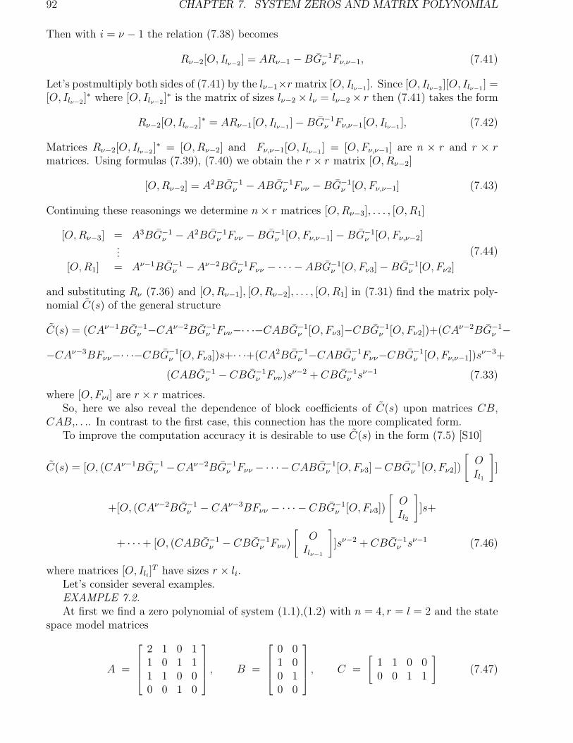
92 CHAPTER 7. SYSTEM ZEROS AND MATRIX POLYNOMIAL
Then with i = ν − 1 the relation (7.38) becomes
Rν−2[O, Ilν−2] = ARν−1 −BG−1
ν Fν,ν−1, (7.41)
Let’s postmultiply both sides of (7.41) by the lν−1×r matrix [O, Ilν−1]. Since [O, Ilν−2
][O, Ilν−1] =
[O, Ilν−2]∗ where [O, Ilν−2
]∗ is the matrix of sizes lν−2 × lν = lν−2 × r then (7.41) takes the form
Rν−2[O, Ilν−2]∗ = ARν−1[O, Ilν−1
] − BG−1ν Fν,ν−1[O, Ilν−1
], (7.42)
Matrices Rν−2[O, Ilν−2]∗ = [O,Rν−2] and Fν,ν−1[O, Ilν−1
] = [O,Fν,ν−1] are n × r and r × rmatrices. Using formulas (7.39), (7.40) we obtain the r × r matrix [O,Rν−2]
[O,Rν−2] = A2BG−1ν − ABG−1
ν Fνν −BG−1ν [O,Fν,ν−1] (7.43)
Continuing these reasonings we determine n× r matrices [O,Rν−3], . . . , [O,R1]
[O,Rν−3] = A3BG−1ν −A2BG−1
ν Fνν −BG−1ν [O,Fν,ν−1] − BG−1
ν [O,Fν,ν−2]...
[O,R1] = Aν−1BG−1ν −Aν−2BG−1
ν Fνν − · · · −ABG−1ν [O,Fν3] −BG−1
ν [O,Fν2]
(7.44)
and substituting Rν (7.36) and [O,Rν−1], [O,Rν−2], . . . , [O,R1] in (7.31) find the matrix poly-nomial C(s) of the general structure
C(s) = (CAν−1BG−1ν −CAν−2BG−1
ν Fνν−· · ·−CABG−1ν [O,Fν3]−CBG−1
ν [O,Fν2])+(CAν−2BG−1ν −
−CAν−3BFνν−· · ·−CBG−1ν [O,Fν3])s+· · ·+(CA2BG−1
ν −CABG−1ν Fνν−CBG−1
ν [O,Fν,ν−1])sν−3+
(CABG−1ν − CBG−1
ν Fνν)sν−2 + CBG−1
ν sν−1 (7.33)
where [O,Fνi] are r × r matrices.So, here we also reveal the dependence of block coefficients of C(s) upon matrices CB,
CAB,. . .. In contrast to the first case, this connection has the more complicated form.To improve the computation accuracy it is desirable to use C(s) in the form (7.5) [S10]
C(s) = [O, (CAν−1BG−1ν −CAν−2BG−1
ν Fνν − · · ·−CABG−1ν [O,Fν3]−CBG−1
ν [O,Fν2])
[
OIl1
]
]
+[O, (CAν−2BG−1ν − CAν−3BFνν − · · · − CBG−1
ν [O,Fν3])
[
OIl2
]
]s+
+ · · ·+ [O, (CABG−1ν − CBG−1
ν Fνν)
[
OIlν−1
]
]sν−2 + CBG−1ν sν−1 (7.46)
where matrices [O, Ili]T have sizes r × li.
Let’s consider several examples.EXAMPLE 7.2.
At first we find a zero polynomial of system (1.1),(1.2) with n = 4, r = l = 2 and the statespace model matrices
A =
2 1 0 11 0 1 11 1 0 00 0 1 0
, B =
0 01 00 10 0
, C =
[
1 1 0 00 0 1 1
]
(7.47)

7.2. MARKOV’S PARAMETER MATRICES 93
Sincerank[B,AB,A2B,A3B] = rank[B,AB] = 4
then ν = 2, n = rν. and the system is reduced to Asseo’s canonical form (7.1) with the matricesF and G of the following structure
F =
[
O I2F21 F22
]
, G =
[
OI2
]
(7.48)
where I2 is the 2 × 2 unit matrix, F21, F22 are 2 × 2 submatrices. Using (7.33) we write
C(s) = (CAB − CBF22) + CBs (7.49)
To determine F22 we need at first to find the 4 × 4 transformation matrix N that reduces thesystem to Asseo’s canonical form. By formulas of Section 1.2.3 we find
N =
[
N1
N2
]
(7.50)
where an 2 × 4 matrix N2 is calculated from (1.54)
N2 = [O, I2][B,AB]−1 (7.51)
and an 2 × 4 matrix N1 is found from (1.49)
N1 = N2A (7.52)
Determining
[B,AB]−1 =
0 1 0 −1−1 0 1 0
1 0 0 00 0 0 1
N2 =
[
1 0 0 00 0 0 1
]
, N1 = N2A =
[
2 1 0 10 0 1 0
]
we obtain from (7.50)
N =
1 0 0 00 0 0 12 1 0 10 0 1 0
Then using the relation F = NAN−1 we calculate
F21 =
[
1 1−1 −1
]
, F22 =
[
2 21 0
]
Substituting F22 into (7.49) and calculating CB, CAB yields the following matrix polynomial
C(s) =
([
1 11 1
]
−[
2 20 1
])
+
[
1 00 1
]
s =
[
−1 −10 1
]
+
[
1 00 1
]
s (7.53)
Thus the zero polynomial isψ(s) = detC(s) = s2 − 1 (7.54)

94 CHAPTER 7. SYSTEM ZEROS AND MATRIX POLYNOMIAL
To check the results obtained we calculate the determinant of the system matrix
detP (s) = det
s− 2 −1 0 −1 0 0−1 s −1 −1 −1 0−1 −1 s 0 0 −10 0 −1 s 0 01 1 0 0 0 00 0 1 1 0 0
= s2 − 1
EXAMPLE 7.3.
Let’s determine a zero polynomial of the system from Example 7.1. Since this system hasn = 4, r = l = 2, ν = 3, l1 = l2 = 1, l3 = 2 then using (7.45) we obtain the general structureof the matrix C(s)
C(s) = (CA2BG−1ν −CABG−1
ν [O,F33]−CBG−1ν [O,F32])+(CABG−1
ν −CBG−1ν F33)s+CBG
−1ν s2
(7.55)where F32, F33 are 2 × 1 and 2 × 2 matrices respectively. For calculating F32, F33 and G−1
ν weuse the formulas from (7.2) (F = NAN−1 and G = NBM) with N (1.93) and M (1.90) (seeExample 1.3). We result in
F32 =
[
11
]
, F33 =
[
2 01 1
]
, Gν =
[
1 00 1
]
(7.56)
Since M = I2 then Gν = GνMT = Gν . Calculating
CB =
[
1 01 1
]
, CAB =
[
2 −13 1
]
, CA2B =
[
3 27 3
]
and substituting these matrices and matrices (7.56) in (7.55) we obtain
C(s) =
[
0 20 0
]
+
[
0 −10 0
]
s+
[
1 00 1
]
s2 (7.57)
The matrix polynomial (7.57) coincides with one obtained in Example 7.1.
7.3 A number of zeros
In this section we obtain several upper bounds of a system zeros number in terms of thematrices CB, CAB,... and the controllability characteristics of the pair (A,B).
At first we consider controllable system (1.1),(1.2) with equal number of independent inputsand outputs ( r = l, rankB = rankC = r). System zeros of this system coincide with zeros ofthe polynomial ψ(s) = sn−rνdet(C(s)) where the r × r matrix C(s)
C(s) = [O,C1] + [O,C2]s+ · · · + [O,Cν−1]sν−2 + Cνs
ν−1 (7.58)
is the nonmonic matrix polynomial of the degree ν−1 with r×r matrices [O,Ci], i = 1, 2, . . . , νof dimensions r × r. Here r × li submatrices Ci, i = 1, 2, . . . , ν are defined from the relation(7.46) as
Cν = CBG−1ν
Cν−1 = (CABG−1ν − CBG−1
ν Fνν)
[
OIlν−1
]
...
C1 = (CAν−1BG−1ν − CAν−2BG−1
ν Fνν − · · · − CBG−1ν [O,Fν2])
[
OIl1
]
(7.59)
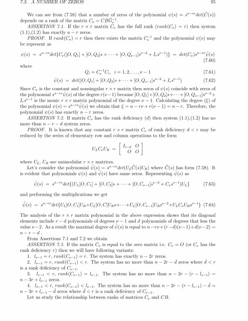
7.3. A NUMBER OF ZEROS 95
We can see from (7.58) that a number of zeros of the polynomial ψ(s) = sn−rνdet(C(s))depends on a rank of the matrix Cν = CBG−1
ν .ASSERTION 7.1. If the r × r matrix Cν has the full rank (rank(Cν) = r) then system
(1.1),(1.2) has exactly n− r zeros.PROOF. If rank(Cν) = r then there exists the matrix C−1
ν and the polynomial ψ(s) maybe represent as
ψ(s) = sn−rνdetCν([O,Q1] + [O,Q2]s+ · · ·+ [O,Qν−1]sν−2 + Irs
ν−1) = det(Cν)sn−rνψ(s)
(7.60)where
Qi = C−1ν Ci, i = 1, 2, . . . , ν − 1 (7.61)
ψ(s) = det([O,Q1] + [O,Q2]s+ · · · + [O,Qν−1]sν−2 + Irs
ν−1) (7.62)
Since Cν is the constant and nonsingular r× r matrix then zeros of ψ(s) coincide with zeros ofthe polynomial sn−rνψ(s) of the degree r(ν−1) because [O,Q1]+[O,Q2]s+· · ·+[O,Qν−1]s
ν−2+Irs
ν−1 is the monic r × r matrix polynomial of the degree ν − 1. Calculating the degree (ξ) ofthe polynomial ψ(s) = sn−rνψ(s) we obtain that ξ = n− rν + r(ν − 1) = n− r. Therefore, thepolynomial ψ(s) has exactly n− r zeros.
ASSERTION 7.2. If matrix Cν has the rank deficiency (d) then system (1.1),(1.2) has nomore than n− r − d system zeros.
PROOF. It is known that any constant r × r matrix Cν of rank deficiency d < r may bereduced by the series of elementary row and column operations to the form
ULCνUR =
[
Ir−d OO O
]
where UL, UR are unimodular r × r matrices.Let’s consider the polynomial ψ(s) = sn−rνdet(ULC(s)UR) where C(s) has form (7.58). It
is evident that polynomials ψ(s) and ψ(s) have same zeros. Representing ψ(s) as
ψ(s) = sn−rνdet(UL[O,C1] + [O,C2]s+ · · ·+ [O,Cν−1]sν−2 + Cνs
ν−1)UL (7.63)
and performing the multiplications we get
ψ(s) = sn−rνdetUL[O,C1]UR+UL[O,C]URs+· · ·+UL[O,Cν−1]URsν−2+ULCνURs
ν−1 (7.64)
The analysis of the r × r matrix polynomial in the above expression shows that its diagonalelements include r− d polynomials of degrees ν − 1 and d polynomials of degrees that less thevalue ν−2. As a result the maximal degree of ψ(s) is equal to n−rν+(r−d)(ν−1)+d(ν−2) =n− r − d .
From Assertions 7.1 and 7.2 we obtainASSERTION 7.3. If the matrix Cν is equal to the zero matrix i.e. Cν = O (or Cν has the
rank deficiency r) then we will have following variants:1. lν−1 = r, rank(Cν−1) = r. The system has exactly n− 2r zeros.2. lν−1 = r, rank(Cν−1) < r. The system has no more than n − 2r − d zeros where d < r
is a rank deficiency of Cν−1.3. lν−1 < r, rank(Cν−1) = lν−1. The system has no more than n − 2r − (r − lν−1) =
n− 3r + lν−1 zeros.4. lν−1 < r, rank(Cν−1) < lν−1. The system has no more than n − 2r − (r − lν−1) − d =
n− 3r + lν−1 − d zeros where d < r is a rank deficiency of Cν−1.Let us study the relationship between ranks of matrices Cν and CB.

96 CHAPTER 7. SYSTEM ZEROS AND MATRIX POLYNOMIAL
ASSERTION 7.4. For controllable system (1.1), (1.2) with l ≥ r the following rank equalityis true
rankCν = rank(CB) (7.65)
The proof follows from the equality Cν = CBG−1ν because the r × r matrix Gν = GνM
T
is nonsingular one.Using Assertion 7.4 and formula (7.59) we can reformulate Assertions 7.1 - 7.3 in terms of
CB, CAB, . . ..THEOREM 7.5. A number of system zeros of controllable system (1.1), (1.2) with r = l is
defined via ranks of matrices CB, CAB, . . . as follows:1. if rank(CB) = r then the system has exactly n− r zeros.2. if the matrix CB has a rank deficiency d then the system has no more than n − r − d
zeros.3. if the matrix CB is the zero matrix then:3.1. if lν−1 = r and rank(CAB) = r then the system has exactly n− 2r zeros,3.2. if lν−1 = r and rank(CAB) < r with a rank deficiency d < r then the system has no
more than n− 2r − d zeros,3.3. if lν−1 < r and rank(CAB) = lν−1 then the system has no more than n − 3r + lν−1
zeros,3.4. if if lν−1 < r and rank(CAB) < lν−1 with a rank deficiency d < r then the system
has no more than n− 3r + lν−1 − d zeros. and etc.Let’s consider the system with an unequal number of inputs and outputs. For definiteness
we assume l > r. By Theorem 7.2 system zeros coincide with zeros of a greatest commondivisor of all nonzero minors of the order r of the l × r polynomial matrix sn−rνdetC(s). Asthere are several such minors then we may get only upper bounds on a number of zeros thatfollow from Assertions 7.1 - 7.3 and Theorem 7.5. We select the most important cases.
COROLLARY 7.4. There are following upper bounds on a number of system zeros ofcontrollable system (1.1),(1.2) with l > r :
1. if rank(CB) = r then the system has no more than n− r zeros.2. if the matrix CB has a rank deficiency d then the system has no more than n − r − d
zeros.3. if CB is equal to the zero matrix then:3.1. if lν−1 = r and rank(CAB) = r then the system has no more than n− 2r zeros,
The next cases coincide with the corresponding points of Theorem 7.5.In conclusion we consider conditions when system (1.1),(1.2) with n = rν has no zeros. It
follows from Ci (7.59) and Corollary 7.4 that zeros are absent if the matrix CAν−1B has a fullrank and matrices CB,CAB, . . . are zero matrices. The last condition is true if
C[B,AB, . . . , Aν−2B] = O
Denoting subspaces, which are formed from linear independent rows of C and columns of then × (n − r) matrix [B,AB, . . . , Aν−2B] by Rc and Rν−2 respectively we obtain from the lastreasonings.
ASSERTION 7.5. If the subspace Rc is orthogonal to the subspace Rν−2 and rank(CAν−1B) =r then system (1.1), (1.2) with l ≥ r and n = rν has no system zeros.
REMARK 7.4. If all matrices CAiB, i = 0, 1, . . . , ν− 1, are zero matrices in the mentionedsystem then the system has zeros everywhere on the complex plan. Such a system is known asthe degenerate system [D4] 2.
2In this case a zero polynomial is identically equal to zero. That implies that system zeros coincide with thewhole complex plane.

7.4. ZERO DETERMINATION VIA LOWER ORDER MATRIX PENCIL 97
The completely controllable system with C 6= O and r = 1, ν = n is always the non-degenerate system. Indeed, the subspace Rν−1, which is formed from columns of matrix[b, Ab, . . . , An−1b], coincides with the complete state space. Therefore, an intersection of Rc
and Rν−1 is not the empty subspace.REMARK 7.5. A similarly way may be used to derive on a number of zeros of system (1.1),
(1.2) with l < r.
7.4 Zero determination via lower order
matrix pencil
In this section we reduce the problem of the zero calculation to eigenvalues problem for amatrix pencil of order n−r [S8]. We restrict our study by system (1.1), (1.2) with equal numberof inputs and outputs. The method is based on constructing the generalized block companionmatrix of the structure (1.25) for the matrix polynomial C(s) (7.5).
We will consider two cases.CASE 1. CB is nonsingular matrix. Then the r × r matrix Cν = CBG−1
ν also has afull rank and there exists the matrix C−1
ν . The matrix polynomial C(s) can be represented asfollows
C(s) = Cν[O, Tν−1] + [O, Tν−2]s+ · · · + [O, T1]sν−2 + Irs
ν−1 (7.66)
where r × li submatrices Tν−i are defined by the formula
Tν−i = C−1ν Ci, i = 1, 2, . . . , ν − 1 (7.67)
The expression in brackets in (7.66) coincides with the matrix polynomial (1.19) with p = ν−1and Ti = [O, Ti], i = 1, 2, . . . , ν − 1.
Let’s find a generalized block companion matrix for
Φ(s) = [O, Tν−1] + [O, Tν−2]s + · · ·+ [O, T1]sν−2 + Irs
ν−1 (7.68)
We need to emphasis that here lν−1 = r, hence the r × r block [O, T1] coincides with the r × rmatrix T1 and the structure of (7.68) completely coincides with (1.19). Otherwise, (lν−1 < r)the structure of (7.68) is distinguished from (1.19) by the block [O, T1]. We consider these casesseparately.
If lν−1 = r and [O, T1] = T1 then we get the generalized block companion n × n matrix ofthe form (1.25) with p = ν−1 and n = l1 + l2 + · · ·+ lν−1 = n− r (see Sect 1.2.1). Let’s denotethis matrix as P
P =
E. . . . . . . . . . . . . . . . . . . . . .
−Tν−1,−Tν−2, . . . ,−T1
(7.69)
where the (n− r − lν−1) × (n− r) block E has the following form
E =
O E1,2 O · · · OO O E2,3 · · · O...
......
. . ....
O O O · · · Eν−2,ν−1
(7.70)
with li × li+1 submatrices Ei,i+1 = [O, Ili].
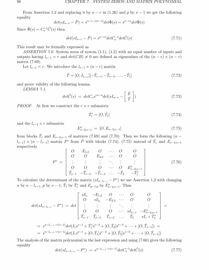
98 CHAPTER 7. SYSTEM ZEROS AND MATRIX POLYNOMIAL
From Assertion 1.2 and replacing n by n− r in (1.26) and p by ν − 1 we get the followingequality
det(sIn−r − P ) = sn−r−r(ν−1)detΦ(s) = sn−rνdetΦ(s)
Since Φ(s) = C−1ν C(s) then
det(sIn−r − P ) = sn−rνdetC−1ν detC(s) (7.71)
This result may be formally expressed asASSERTION 7.6. System zeros of system (1.1), (1.2) with an equal number of inputs and
outputs having lν−1 = r and det(CB) 6= 0 are defined as eigenvalues of the (n − r) × (n − r)matrix (7.69).
Let lν−1 < r. We introduce the lν−1 × (n− r) matrix
T = [O, Ilν−1][−Tν−1,−Tν−2, . . . ,−T1] (7.72)
and prove validity of the following lemma.LEMMA 7.1.
detC(s) = detCνsrν−ndet(sIn−r −
[
E
T
]
) (7.73)
PROOF. At first we construct the r × r submatrix
T ∗
1 = [O, T1] (7.74)
and the lν−2 × r submatrixEoν−2,ν−1 = [O,Eν−2,ν−1] (7.75)
from blocks T1 and Eν−2,ν−1 of matrices (7.69) and (7.70). Then we form the following (n −lν−1) × (n − lν−1) matrix P ∗ from P with blocks (7.74), (7.75) instead of T1 and Eν−2,ν−1
respectively
P ∗ =
O E1,2 O · · · O OO O E2,3 · · · O O...
......
. . ....
...O O O · · · O Eo
ν−2,ν−1
Tν−1 −Tν−2 −Tν−3 . . . −T2 −T ∗
1
(7.76)
To calculate the determinant of the matrix (sIn−lν−1− P ∗) we use Assertion 1.2 with changing
n by n− lν−1, p by ν − 1, T1 by T ∗
1 and Ep−1,p by Eoν−2,ν−1. Thus
det(sIn−lν−1− P ∗) = det
sIl1 −E1,2 O · · · O OO sIl2 −E2,3 · · · O O...
......
. . ....
...O O O · · · sIlν−2
−Eoν−2,ν−1
Tν−1 Tν−2 Tν−3 . . . T2 sIr + T ∗
1
=
= sn−lν−1−r(ν−1)det(Irsν−1 + T ∗
1 sν−2 + [O, T2]s
ν−3 + · · ·+ [O, Tν−1]) =
= sn−lν−1−r(ν−1)det(Irsν−1 + [O, T1]s
ν−2 + [O, T2]sν−3 + · · ·+ [O, Tν−1])
The analysis of the matrix polynomial in the last expression and using (7.66) gives the followingequality
det(sIn−lν−1− P ∗) = sn−lν−1−r(ν−1)detC−1
ν detC(s) (7.77)

7.4. ZERO DETERMINATION VIA LOWER ORDER MATRIX PENCIL 99
On the other hand substituting (7.74) and (7.75) into the right-hand side of (7.76) gives
det(sIn−lν−1− P ∗) =
sIl1 −E1,2 O · · · O OO sIl2 −E2,3 · · · O O...
......
. . ....
...O O O · · · sIlν−2
−[O,Eν−2,ν−1]
Tν−1 Tν−2 Tν−3 . . . T2 sIr + [O, T1]
(7.78)
Partitioning submatrices Ti, i = 1, 2, . . . , ν − 1 as
Ti =
T 1i
T 2i
r − lν−1
lν−1
(7.79)
where blocks T 1i , T 2
i have r− lν−1 and lν−1 rows respectively we find the structure of the matrixsIr + [O, T1]
sIr + [O, T1] = sIr +
O T 1i
O T 2i
=
sIq T 1i
O sIlν−1+ T 2
i
(7.80)
where q = r − lν−1. Substituting (7.79) and (7.80) into (7.78)
det(sIn−lν−1− P ∗) =
sIl1 −E1,2 O · · · O O OO sIl2 −E2,3 · · · O O O...
......
. . ....
......
O O O · · · sIlν−2O −Eν−2,ν−1
T 1ν−1 T 1
ν−2 T 1ν−3 . . . T 1
2 sIq T 11
T 2ν−1 T 2
ν−2 T 2ν−3 . . . T 2
2 O sIlν−1+ T 2
1
(7.81)
and calculating the determinant of the block matrix we get
det(sIn−lν−1− P ∗) = sqdet
sIl1 −E1,2 O · · · O OO sIl2 −E2,3 · · · O O...
......
. . ....
...O O O · · · sIlν−2
−Eν−2,ν−1
T 2ν−1 T 2
ν−2 T 2ν−3 . . . T 2
2 sIlν−1+ T 2
1
Using notations (7.70), (7.72) and relations: q = r− lν−1, l1 + l2 + · · ·+ lν−2 + lν−1 = n− r wecan rewrite the last equality as follows
det(sIn−lν−1− P ∗) = sr−lν−1det(sIn−r −
[
E
T
]
) (7.82)
Equating right-hand sides of (7.82) and (7.77) yields
sn−lν−1−r(ν−1)detC−1ν detC(s) = sr−lν−1det(sIn−r −
[
E
T
]
)

100 CHAPTER 7. SYSTEM ZEROS AND MATRIX POLYNOMIAL
The last equality proves the lemma.The following result follows immediately from Assertion 7.6, Lemma 7.1 and formulas (7.67)
and (7.72).THEOREM 7.6. System zeros of system (1.1), (1.2) with an equal number of inputs and
outputs and det(CB) 6= 0 are defined as eigenvalues of the (n−r)× (n−r) matrix
[
E
T
]
where
the lν−1 × (n− r) submatrix T satisfies to the following formula
T =
−C−1ν [C1, C2, . . . Cν−1] , lν−1 = r
−[O, Ilν−1]C−1
ν [C1, C2, . . . Cν−1] , lν−1 < r(7.83)
CASE 2. CB is singular matrix. Hence, the r × r matrix Cν = CBG−1ν is also singular
one. Let’s introduce the (n− lν−1) × (n− lν−1) matrix
In−lν−1=
[
Iβ OO Cν
]
, β = l1 + l2 + · · ·+ lν−2 (7.84)
and the r × (n− r) matrixC∗ = [C1, C2, . . . , Cν−1] (7.85)
LEMMA 7.2. If lν−1 = r then the following equality is true
det(sIn−lν−1−[
E−C∗
]
) = sn−lν−1−r(ν−1)det([O,C1] + [O,C2]s+ · · ·+ [O,Cν−1]sν−2 +Cνs
ν−1)
(7.86)where the (n− r − lν−1) × (n− r) submatrix E is defined from (7.70).
PROOF. To calculate the determinant in the left-hand side of (7.86) we partition the
matrix sIn−lν−1−[
E−C∗
]
into four blocks similarly to ones in (1.27), (1.28) with p = ν − 1
and find a determinant of the resulting block matrix
det(In−lν−1−[
E−C∗
]
) = det
sIl1 −E1,2 O · · · O OO sIl2 −E2,3 · · · O O...
......
. . ....
...O O O · · · sIlν−2
−Eν−2,ν−1
C1 C2 C3 . . . Cν−1 sCν + Cν−1
=
= s(n−lν−1)−rdet(sCν+Cν−1+[C1, C2, . . . , Cν−2]
sIl1 −E1,2 · · · OO sIl2 · · · O...
.... . .
...O O · · · sIlν−2
−1
OO...
Eν−2,ν−1
) =
= s(n−lν−1)−rdet(sCν + Cν−1 + [C1, C2, . . . , Cν−2]
s1−ν [O, Il1]s2−ν [O, Il2]
...s−1[O, Ilν−1
]
) =
s(n−lν−1)−rdet(sCν + Cν−1 + [O,Cν−2]s−1 + · · ·+ [O,C2]s
3−ν + [O,C1]s2−ν) =
= sn−lν−1−r(ν−1)det([O,C1] + [O,C2]s + · · ·+ [O,Cν−1]sν−2 + Cνs
ν−1)

7.4. ZERO DETERMINATION VIA LOWER ORDER MATRIX PENCIL 101
The lemma has been proved.Let lν−1 < r. We introduce the r × r matrix
Cν−1 = [O,Cν−1] (7.87)
and the lν−2×r submatrix Eoν−2,ν−1 of the form (7.75). The following equality is true by Lemma
7.2
det(sIn−lν−1−
E. . . . . . . . . . . . . . . . . . . . . . . . . . . .−C1,−C2, . . . ,−Cν−2,−Cν−1
) =
= sn−lν−1−r(ν−1)det([O,C1] + [O,C2]s + · · ·+ [O,Cν−1]sν−2 + Cνs
ν−1) (7.88)
where the β× (n− lν−1) matrix E (β = l1 + l2 + · · ·+ lν−2) has the form (7.69) with Eν−2,ν−1 =Eoν−2,ν−1.
Recalling that system zeros of controllable system (1.1), (1.2) with l = r are equal to zerosof the polynomial
ψ(s) = sn−rνdet([O,C1] + [O,C2]s+ · · ·+ [O,Cν−1]sν−2 + Cνs
ν−1) (7.89)
and substituting det([O,C1] + [O,C2]s+ · · ·+ [O,Cν−1]sν−2 +Cνs
ν−1) from (7.88) in (7.89) weget
ψ(s) = sn−rνsr(ν−1)−n+lν−1det(sIn−lν−1−[
E−C
]
) = slν−1−rdet(sIn−lν−1−[
E−C
]
)
where C = [C1, C2, . . . , Cν−1, Cν−1]. This result can be formally stated asTHEOREM 7.7. System zeros of system (1.1), (1.2) with an equal number of inputs and
outputs coincide with generalized eigenvalues of the (n− lν−1)×(n− lν−1) regular matrix pencil
Z(s) = s
[
Iβ OO Cν
]
+
−E. . . . . . . . . . . . . . . . . . . . . . . . .C1, C2, . . . , Cν−2, [O,Cν−1]
(7.90)
without r − lν−1 generalized eigenvalues in the origin. In (7.90) the β × (n − lν−1) matrix Ehas the form (7.70) with the lν−2 × r submatrix Eν−2,ν−1 = [O,Eν−2,ν−1] (see (7.75)).
COROLLARY 7.5. If lν−1 = r then system zeros of (1.1), (1.2) with an equal number ofinputs and outputs are defined as generalized eigenvalues of the (n−r)× (n−r) regular matrixpencil
Z(s) = s
[
Iβ OO Cν
]
+
−E. . . . . . . . . . . . . . .C1, C2, . . . , Cν−1
(7.91)
where the β × (n− r) matrix E has the form (7.70).We illustrate the method by the following examples.EXAMPLE 7.3. Let us find zeros of system (1.1), (1.2) with n = 4, r = l = 2 and state-space
model matrices
A =
2 1 0 00 1 0 10 2 0 01 1 0 0
, B =
1 00 00 00 1
, C =
[
1 0 0 00 0 1 1
]
(7.92)

102 CHAPTER 7. SYSTEM ZEROS AND MATRIX POLYNOMIAL
In Example 1.3 (see Sect 1.2.3.) it has been shown that this system has ν = 3, l1 = l2 = 1, l3 =2 and following matrices N and N−1
N =
0 0 0.5 00 1 0 01 0 0 00 1 0 1
, N−1 =
0 0 1 00 1 0 02 0 0 00 −1 0 1
We calculate
CN−1 =
[
1 0 0 00 0 1 1
]
N−1 =
[
0 0 1 02 −1 0 1
]
(7.93)
and partition this matrix on three blocks C1, C2, C3 of dimensions r× l1 = 2×1, r× l2 = 2×1,r × l3 = 2 × 2 respectively
CN−1 = [C1, C2, C3] =
02
...
...
0−1
...
...
1 00 1
Since CB =
[
1 00 1
]
is the nonsingular matrix then we need to use Theorem 7.6 to calculate
system zeros. Using formula (7.70) we form the (n − r − lν−1) × (n − r) submatrix E. Sinceν = 3, l1 = l2 = 1, l3 = 2 then n − r − lν−1 = 1, n − r = 2, and Eν−2,ν−1 = E12 is the 1 × 1submatrix that equals to 1. Thus, we get
E = [0 1]
and by formula (7.83) calculate
T = −[O, Il2]C−13 [C1, C2] = −[0 1]
[
0 02 −1
]
= [−2 1]
The matrix
[
E
T
]
of the order n− r = 2 becomes
[
E
T
]
=
[
0 1−2 1
]
It has the characteristic polynomial
ψ(s) = det
[
s −12 s− 1
]
= s2 − s+ 2
that is equal to the zero polynomial of the present system.For testing we compute the only minor of the system matrix P (s)
detP (s) = det
s− 2 −1 0 0 −1 00 s− 1 0 −1 0 00 −2 s 0 0 0−1 −1 0 s 0 −11 0 0 0 0 00 0 1 1 0 0

7.4. ZERO DETERMINATION VIA LOWER ORDER MATRIX PENCIL 103
We have been obtained the same result.EXAMPLE 7.4.
Let the model (7.92) has the following output matrix
C =
[
1 −1 1 01 0 0 0
]
Since in this case the matrix N is same as above then
CN−1 =
[
1 −1 1 01 0 0 0
]
N−1 =
[
2 −1 1 00 0 1 0
]
(7.94)
Using above calculated controllability characteristics: ν = 3, l1 = l2 = 1, l3 = 2 we partitionthe matrix (7.94) into three blocks C1, C2, C3 of the sizes 2 × 1, 2 × 1, 2 × 2 respectively
CN−1 = [C1, C2, C3] =
20
...
...
−10
...
...
1 01 0
(7.95)
In this case the matrix CB =
[
1 01 0
]
is singular one. Thus, to calculate system zeros we need
to use Theorem 7.7. We form the lν−2 × r submatrix Eoν−2,ν−1 = [O,Eν−2,ν−1] and the r × r
submatrix [O,Cν−1]. Since r = 3, lν−1 = l1 = 1, ν − 2 = 1, ν − 1 = 2 then by the formula(7.75) we find
Eo1,2 =
[
O E1,2
]
=[
0 1]
(7.96)
The 2 × 2 matrix [O,Cν−1] = [O,C2] with the 2 × 1 block C2 from (7.95) is
[O,Cν−1] = [O,C2] =
00
...
...
−10
To form the β× (n− lν−1) matrix E and the (n− lν−1)× (n− lν−1) matrix In−lν−1we use (7.96)
and (7.84). Since ν = 3, β = l1 + · · · + lν−2 = l1 = 1, n− lν−1 = 4 − 1 = 3 then
E = [O,Eo1,2] = [0 0 1]
In−lν−1= In−l2 = I3 =
[
I1 OO C3
]
=
1 0 00 1 00 1 0
We result in the following matrix pencil
Z(s) = s
[
I1 OO C3
]
+
−E. . . . . . . . . .C1, [O,C2]
= s
1 0 00 1 00 1 0
+
0 0 −12 0 −10 0 0
having the following characteristic polynomial
detZ(s) = det(s
1 0 00 1 00 1 0
+
0 0 −12 0 −10 0 0
) = s2 − 2s
According to Theorem 7.7 the zero polynomial is
ψ(s) = slν−1−rdetZ(s) = sl2−rdetZ(s) = s−1detZ(s) = s− 2
Hence, the system has the only system zero s = 2.To test we find the determinant of the system matrix P (s) that equal to s− 2. This result
is in agreement with the obtained one.

104 CHAPTER 7. SYSTEM ZEROS AND MATRIX POLYNOMIAL

Chapter 8
Zero computation
In the present chapter we develop several computational techniques. The natural way tocompute invariant and transmission zeros is based on their definitions via the Smith and Smith-McMillan canonical forms for matrices P (s) and G(s) respectively. Decoupling zeros may becalculated by using the Smith form for matrices Pi(s) = [sIn−A,B] and Po(s)
T = [sIn−AT , CT ].This approach is laborious because of operations with polynomial and/or rational matrices.Here we will study alternative methods that are based on efficient numerical procedures andhave the simple computer-aided realization.
For the most part we will consider a system with an equal number of inputs and outputs(r = l). This restriction does not essential because otherwise we can recommend to performtwice the squaring down operation of outputs (if l > r) or inputs (if l < r) and to find systemzeros as an intersection of sets of zeros of squared down systems. Indeed, let for definitenessl > r. Using different r × l matrices E1 and E2 of full ranks we construct two squared downsystems from (1.1), (1.2):
S1 : x = Ax+Bu, y1 = E1CxS2 : x = Ax+Bu, y2 = E2Cx
Zero sets Ω(E1) and Ω(E2) of systems S1 and S2 respectively are calculated via system matricesP1(s) and P2(s) of the following form
Pi(s) =
[
sIn −A −BEiC O
]
, i = 1, 2 (8.1)
It is evident that the intersection
Ω = Ω(E1) ∩ Ω(E2) (8.2)
’almost always’1 is equal to the zero set of system (1.1), (1.2).
8.1 Zero computation via matrix P(s)
Analysis of the system matrix
P (s) =
[
sIn − A −BC O
]
(8.3)
1I.e. the class of systems that don’t possess such property is either empty or lies on a hypersurface of theparameter space of (A,B,C) [D4].
105

106 CHAPTER 8. ZERO COMPUTATION
shows that the complete set of system zeros is formed as the set of complex s for which thenormal rank of (8.3) is locally reduced. For the system with r = l and non identically zerodetP (s) we can consider the matrix (8.3) as the regular [G1] pencil of matrices
P (s) = sD + L (8.4)
where
L =
[
−A −BC O
]
, D =
[
In OO O
]
(8.5)
Thus, the problem is reduced to calculating generalized eigenvalues of the regular matrix pencil(8.4). These generalized eigenvalues coincide with finite s for which there exist a nontrivialsolution of the equation (sD + L)q = 0 where q is an n + r vector [P1]. To calculategeneralized eigenvalues we can apply QZ algorithm [P1]. Moreover, the special modification[M6] of this algorithm may be used for a singular matrix D. In [L3] this modification wassuccessfully applied to calculating zeros via the matrix pencil (8.4).
The advantage of the mentioned approach is its numerical stability because of effectivenessof QZ algorithm. The main shortcoming is associated with separating decoupling zeros fromtransmission zeros.
To overcome this problem we may use the method proposed by Porter [P7]. This approachproposes at first to solve twice the QZ problem for the regular (n+ r + l) × (n+ r + l) matrixpencil
s
In O OO O OO O O
+
−A O B−C Il OO Ki Ir
(8.6)
where Ki, i = 1, 2 are some full rank matrices with bounded elements. Indeed, using theformula Shura [G1] we can calculate
det
sIn − A O B−C Il OO Ki Ir
= det(sIn −A− BKiC), i = 1, 2 (8.7)
Thus, applying matrices Ki (i = 1, 2) in (8.6) is equivalent to introducing a proportionaloutput feedback u = Kiy into the system: x = Ax + Bu, y = Cx. Such feedback shiftsonly controllable and observable eigenvalues of the matrix A. Uncontrollable and unobservableeigenvalues are the invariants under the proportional output feedback and they are decouplingzeros of the system (see Sections 2.4, 5.3). Hence, those generalized eigenvalues of the problem(8.6), which are not changed for different matrices Ki (i = 1, 2) coincide with decoupling zerosof system (1.1), (1.2) and a set of decoupling zeros Ωd is almost always computed from theintersection
Ωd = Ω(K1) ∩ Ω(K2) (8.8)
where Ω(Ki), i = 1, 2 are sets of generalized eigenvalues of matrix pencils (8.6).If the whole set of system zeros Ω has been computed by somehow method then from the
unionΩ = Ωd ∪ Ωt (8.9)
we can separate the set of transmission zeros Ωd from the set of decoupling zeros.For calculating the set Ω for a system with an unequal number of inputs and outputs (r 6= l)
we can use the following strategy. At first the QZ problem is twice solved for following regularmatrix pencils of the order n+min(r, l)
s
[
In OO O
]
+
[
−A −BEiC O
]
, if l > r (8.10)

8.1. ZERO COMPUTATION VIA MATRIX P(S) 107
s
[
In OO O
]
+
[
−A −BEiC O
]
, if l < r (8.11)
where Ei, i = 1, 2 are some r × l matrices of a full rank with bounded elements. In view ofpreceding reasoning these pencils correspond to system matrices P1(s) and P2(s) of squareddown systems: P1(s) defines the system with squared down outputs and P2(s) defines thesystem with squared down inputs. Let’s denote zero sets of the first and second squared downsystems by Ω1(Ei) and Ω1(Ei) respectively. It is evident that the zero set of original system(1.1), (1.2) can be calculated from the following intersections
Ω = Ω1(E1) ∩ Ω1(E2) for l > r (8.12)
Ω = Ω2(E1) ∩ Ω2(E2) for l < r (8.13)
In the work [7] it is presented the following computational method for a system with l ≥ r: tosolve twice the QZ problem for the following regular (n+ r + l) × (n+ r + l) matrix pencil
s
In O OO O OO O O
+
−A O B−C Il OO Ki O
(8.14)
which is distinguished from the matrix pencil (8.6) by the only block. The set Ω of systemzeros is calculated from the following intersection
Ω = Ω∗(K1) ∩ Ω∗(K2) (8.15)
where Ω∗(Ki) (i = 1, 2) are sets of generalized eigenvalues of the matrix pencil (8.14).Let us show that the present method actually computes the full set of system zeros. Indeed,
interchanging the second and third block rows and columns of the matrix pencil (8.14) andusing the formula Shura [G1] we calculate the determinant of (8.14)
det
sIr − A O B−C Il OO Ki O
= det
sIr − A B OO O Ki
−C O Il
=
= det
[
sIr −A BKiC O
]
= (−1)rdet
[
sIr −A −BKiC O
]
(8.16)
It follows from (8.16) that generalized eigenvalues of the regular pencil (8.14) coincide withones of the regular pencil (8.10) with Ki = Ei (i = 1, 2). Therefore, intersection (8.15) givesthe set of system zeros.
The similar procedure may be used when r ≥ l. Here it is applied the following (n + r +l) × (n+ r + l) matrix pencil
s
In O OO O OO O O
+
−A O B−C O OO Ki Ir
(8.17)
having the following determinant
det
sIr − A O B−C O OO Ki Ir
= (−1)ldet
[
sIr −A −BKi
C O
]
(8.18)

108 CHAPTER 8. ZERO COMPUTATION
It follows from (8.18) that generalized eigenvalues of the pencil (8.17) coincide with ones of theregular pencil (8.11) with Ki = Ei (i = 1, 2). Therefore, all previous reasoning are held.
The advantage of this approach is the applicability of the universal QZ algorithm for matrixpencils (8.6), (8.14) or (8.17). Hence, similar computational algorithms and computer softwarecan be used as for computing zeros as for separating different type zeros. But such approachincreases considerably a dimension of the problem. Therefore, when r 6= l it is more preferableto use the QZ procedure for pencils (8.10) or (8.11) of the order n+min(r, l).
8.2 Zero computation based on matrix A+BKC
This approach uses invariance of zeros under a high gain output feedback (see Sect.6.5). Letus remind this property. We consider a close-loop controllable and observable system havingthe following dynamics matrix: A(K) = A + kBKC where K is some arbitrary matrix withlimited elements, k is a real scalar. If k goes to infinity (k → ∞) then n − r eigenvalues ofthe matrix A(k) approach positions of transmission zeros of system (1.1), (1.2) and r remindereigenvalues tend to infinity. Therefore, to calculate zeros we can use the following approach[D4]:
1. Compute n eigenvalues of the matrix A(K) = A+ kBKC for any arbitrary matrix K ofa full rank and a large value of k ≈ 1015.
2. Separate n− r finite eigenvalues that are equal to transmission zeros.This approach may be successfully used for uncontrollable and/or unobservable system. In-
deed, decoupling zeros coincide with limited eigenvalues of the dynamics matrix of a closed-loopsystem that are invariant under a proportional output feedback and the procedure above calcu-lates system zeros of an uncontrollable and/or unobservable system. But here it is necessary toseparate sets of transmission and decoupling zeros. For this purpose we can use, for example,the approach of Section 8.1.
Consequently, for uncontrollable and/or unobservable system (1.1), (1.2) with r = l wepropose the following general procedure:
1. Find finite eigenvalues of the matrix A+kBK1C with k ≈ 1015 and K1 being an arbitrarymatrix of a full rank. Denote these eigenvalues by Ω(K1).
2. Repeat step 1 with another matrix K2. Denote resulted eigenvalues as Ω(K2) .3. From intersection (8.8) calculate decoupling zeros Ωd.4. From union (8.9) calculate transmission zeros Ωt .The advantage of this approach is its simplicity . Moreover, in contrast to the approach of
Sect.8.1, the processed matrices are of small sizes. But low computational accuracy (using alarge number k ≈ 1015) makes difficulties for applicability of this method.
8.3 Zero computation via transfer
function matrix
Now we consider the numerical method proposed by Samash in [S1]. This method is basedon the definition of system zeros of a square system as zeros of the following polynomial ψ(s)(see Sect 5.2, formula (5.11))
ψ(s) = det(sIn −A)det(C(sIn − A)−1B) (8.19)
Let the system has µ zeros, µ ≤ n− r. Then the zero polynomial ψ(s)
ψ(s) = ao + a1s+ · · · + aµsµ (8.20)

8.4. ZERO COMPUTATION VIA MATRIX POLYNOMIAL AND MATRIX PENCIL 109
with unknown real coefficients ai , i = 0, 1, . . . , µ to be found. Substituting in the right-handside of (8.19) µ + 1 different real numbers si, i = 1, 2, ..., µ + 1 that differ from eigenvalues ofthe matrix A we result in the following µ+ 1 real numbers bi, i = 1, 2, ..., µ+ 1
bi = ψ(si) = det(siIn − A)det(C(siIn −A)−1B) (8.21)
Substituting same si into (8.20) we write µ+ 1 equations in the coefficients ai , i = 0, 1, . . . , µ
ψ(si) = ao + a1si + · · · + aµsµi = [1, si, . . . , s
µi ]
aoa1...aµ
(8.22)
Equating the left-hand side of (8.21) to the right-hand side of (8.22) for i = 1, 2, . . . , µ+ 1 weget the following system of linear algebraic equations in unknown ai, i = 0, 1, . . . , µ
1 s1 s21 · · · sµ1
1 s2 s22 · · · sµ2
......
... · · · ...1 sµ+1 s2
µ+1 · · · sµµ+1
aoa1...aµ
=
b1b2...
bµ+1
(8.23)
The square matrix in (8.23) is nonsingular one if si 6= sj (i = 1, 2, . . . , µ+ 1) because it is theVandermonde matrix. Thus, system (8.23) has the only solution in ao, a1, . . . , aµ.
For realization of this method it is necessary to know a number of zeros (µ). For this purposewe can use results of Section 7.3. If it is difficult to find µ then we should change this valueby an upper bound µ ≥ µ. Then we need to separate actual system zeros from zeros of thepolynomial ao + a1s+ · · ·+ aµs
µ by finding such si that reduce the rank of the system matrixP (s).
Thus we can write the following algorithm:
1. Evaluate a number µ or its an upper estimate µ .
2. Assign different si 6= λj (i = 1, 2, . . . , η + 1, j = 1, 2, . . . , n) where λj are eigenvalues ofA, η = µ or η = µ.
3. Calculate bi (i = 1, 2, . . . , η + 1), η = µ or η = µ.
4. Build the Vandermonde matrix (8.23).
5. Calculate ao, a1, . . . , aµ, η = µ or η = µ.
6. If η = µ then ao, a1, . . . , aµ are coefficients of the zero polynomial; otherwise (η = µ),select among zeros of the polynomial ao + a1s+ · · ·+ aµs
µ such z∗i that reduce the rank of thematrix P (s) at s = z∗i .
This method is less laborious than the method of Sect.8.1 because it processes n×nmatrices.But its numerical accuracy depends on accuracy of inverting n× n matrices, which may be illconditioned matrices. Moreover, the separation of system zeros from zeros of the polynomialψ(s) also influences on numerical accuracy.
8.4 Zero computation via matrix
polynomial and matrix pencil
These approaches are based on results of Chapter 7.

110 CHAPTER 8. ZERO COMPUTATION
METHOD 1. To calculate zeros of controllable square system (1.1), (1.2) it is used thedefinition of zeros via the following polynomial
ψ(s) = sn−rνdet([O,C1] + [O,C]s+ · · ·+ [O,Cν−1]sν−2 + Cνs
ν−1) (8.24)
where Ci are r × li submatrices, ν, l1, l2, . . . , lν are the controllability characteristics of thepair (A,B) (see Sect. 7.1 for details). The method is a modification of Samash’s method.We find a zero polynomial ψ(s) in the form (8.24). Then assigning different real numberss1, s2, . . . , sµ+1 that do not coincide with eigenvalues of the matrix A we calculate real numbersbi (i = 1, 2, . . . , µ+ 1)
bi = ψ(si) = sn−rνi det([O,C1] + [O,C]si + · · · + [O,Cν−1]sν−2i + Cνs
ν−1i ) (8.25)
Equating the right-hand side of (8.20) to bi, i = 1, 2, . . . , µ + 1 gives the system of linearequations in ai (i = 0, 1, . . . , µ) used for system zeros calculation.
Above reasonings can be expressed in the following algorithm:1. Determine controllability characteristics of system (1.1), (1.2): ν, l1, l2, . . . , lν (see for-
mulas (1.45), (1.59)) and the n × n transformation matrix N that reduces the pair (A,B) toYokoyama’s (n ≤ rν) or Asseo’s (n = rν) canonical form.
2. Calculate r × li submatrices Ci , i = 1, 2, . . . , ν from the relation [C1, C2, . . . , Cν ] =CN−1.
3. Evaluate a zeros number µ or an upper bound µ from analysis of blocks Cν , Cν−1, . . .(see Sect.7.3).
4. Assign different real numbers si 6= λj (i = 1, 2, . . . , η + 1, j = 1, 2, . . . , n) where λj areeigenvalues of A, η = µ or η = µ.
5. Calculate bi (i = 1, 2, . . . , η + 1) from formula (8.24), η = µ or η = µ.Further see steps 4-6 of the algorithm of Sect 8.3.This algorithm has more steps than the Samash’s method but computational difficulties
are decreased because we operate with matrices of the order n − r + 1 and µ + 1. Moreover,to calculate submatrices Ci we may use formulas of Section 7.2: Cν = CBG−1
ν , Cν−1 =CABG−1
ν − CBG−1ν Fνν and so on. Also the iterative procedure of the work [S10] may be used
to compute Fν1, . . . , Fνν without any inverting an n× n matrix N .METHOD 2. It is based on Theorems 7.6 and 7.7 of Sect.7.4. Zeros are computed via
square matrices of the order n− r or n− lν−1 as follows:1. If the condition det(CB) 6= 0 is satisfied then system zeros are calculated as eigenvalues
of the following (n− r) × (n− r) matrix
Z(s) =
E. . . . . . . . . . . . . . . . . . . . . . . . . . . . .−θC−1
ν [C1, C2, . . . , Cν−2, Cν−1]
(8.26)
where θ = Ir for lν−1 = r or θ = [O, Ilν−1] for lν−1 < r, the (n − 2r) × (n − r) matrix E has
the form (7.70), [C1, C2, . . . , Cν] = CN−1, N is a n × n transformation matrix reducing pair(A,B) to Yokoyama’s canonical form.
2. If det(CB) = 0 then system zeros are generalized eigenvalues of the following matrixpencil of order n− lν−1
Z(s) = s
[
Iβ OO Cν
]
+
−E. . . . . . . . . . . . . . . . . . . . . . . . .C1, C2, . . . , Cν−2, [O,Cν−1]
(8.27)

8.4. ZERO COMPUTATION VIA MATRIX POLYNOMIAL AND MATRIX PENCIL 111
where β = l1 + l2 + · · · + lν−2 = n− r − lν−1, the β × (n− lν−1) matrix E has the form (7.70)with Eν−2,ν−1 = [O,Eν−2,ν−1] being the lν−2 × r submatrix, [C1, C2, . . . , Cν ] = CN−1.
The present approach decreases computational difficulties because it processes square ma-trices of the order n − r or n − lν−1. To calculate submatrices Ci (i = 1, 2, . . . , ν) we alsocan use formulas of Sect.7.2 that allow to avoid inverting an n × n matrix N . For computingeigenvalues or generalized eigenvalues of (8.26) or (8.27) we can use QZ algorithm.
REMARK 8.1. These computational methods are applied to the well conditional controlla-bility matrix YAB = [B,AB, . . . , An−1B]. Otherwise, we can recommend to make the followingoperations:
1. Separate a well conditioned part of YAB,2. Decrease a dimension of the controllability subspace,3. Calculate system zeros of the system obtained. They form the set of invariant zeros.The rest of zeros (input decoupling zeros ) may be found by another approach.

112 CHAPTER 8. ZERO COMPUTATION

Chapter 9
Zero assignment
In this chapter we consider the assignment of system zeros by choosing the output (input)matrix or by using the squaring down operation. This problem is caused by large influence ofsystem zeros on dynamic behavior of any control system. It is known from the classic controltheory that right-half plan zeros create severe difficulties for the control design. Multivariablesystems have similar properties. For example, maximally achievable accuracy of optimal reg-ulators and/or filters is attainable if an open-loop system has not zeros in the right-half partof the complex plane [K4], [K5]. In Section 10 we demonstrate that solvability conditions ofdifferent type tracking problems also contain limitations on system zero locations.
System zeros are invariant under state and/or output proportional feedbacks. They maybe shift only by an appropriate correction of output and/or input matrices.1 We consider twodifferent techniques: the first one shifts an output matrix and second one calculates a squaringdown compensator.
9.1 Zero assignment by selection of output matrix
This approach is based on appropriate choice of an output matrix C of a system and maybe recommended when a freedom ’may still exist to choose that sets of variables are to bemanipulated and what sets to be measured for control purpose’[M1]. For example, an outputmatrix C may be selected in an estimation system where the whole state vector is available formeasurement.
The zero assignment problem by choosing an output matrix has been set up by Rosenbrockin [R1,Theorem 4.1] and briefly is formulated as follows.
Let in given square system (1.1), (1.2) with the completely controllable pair (A,B) we maychoose the r×n matrix C in (1.2). Form the problem : it is necessary to choose a matrix C sothat
1. the pair (A,B) is observable,
2. The Smith-McMillan form M(s) of the r × r transfer function matrix G(s) = C(sIn −A)−1B has assigned numerator polynomials ǫi(s).
Rosenbrock has shown that such C always can be chosen if degrees of assigned ǫi(s) satisfycertain conditions. But there are some restrictions on the choice of the output (measurable)matrix, which also should take into account, for example, a fullness rank of the matrix C, well-posed of the observability matrix ZAC and others. Moreover, Rosenbrock’s necessary conditionson degrees of polynomials ǫi(s) are rather complicated .
1Later we will use only an output matrix for the zero assignment.
113

114 CHAPTER 9. ZERO ASSIGNMENT
Further we will ensure distinct assigned zeros. This restriction on zero locations considerablysimplifies Rosenbrock’s conditions. Also we will ensure fullness of a rank of the matrix Cand several other requirements. The methods are based on works [S6], [S11], which use zerodefinitions via a matrix polynomial and the reduced (lower order) matrix (see Chapter 7).
9.1.1 Iterative method of zero assignment
We consider completely controllable system (1.1) with r independent inputs (rankB = r)and the completely measurable state vector x.
Let us assign n − r 2 distinct real numbers si (i = 1, 2, . . . , n − r) and denote by ψ(s) thefollowing zero polynomial
ψ(s) =n−r∏
i=1
(s− si) (9.1)
We consider the following problem.PROBLEM 1. To choose the r× n output matrix C that assigns zeros of system (1.1) with
the output
y = Cx (9.2)
at desired positions si. Matrix C must also satisfy the following requirements:
(a). the pair (A,B) is observable,
(b). rankC = r (9.3)
Now we find conditions, which assure a solution of the problem. These conditions may beconsidered as a particular case of Rosenbrock’s ones.
THEOREM 9.1. If the pair of matrices (A,B) is controllable and distinct zeros si (i =1, 2, . . . , n− r) do not coincide with eigenvalues of the matrix A then there exists a matrix Cthat ensures both the assigned zero polynomial to system (1.1), (9.2) and the condition (9.3a).
PROOF [S6]. We base on Theorem 4.1 from [R1, p.186] where general zero assignmentconditions are defined.
At first we consider values µ1,µ2,. . . ,µq that are nonzero minimal indices of the singularmatrix pencil (sIn−A,B) with the n× p matrix B (rankB = q ≤ p), 1 ≤ µ1 ≤ µ2 ≤ · · · ≤ µq,µ1 +µ2 + · · ·+µq = n. As it has been studied in [R1], the minimal indices coincide with orderednumbers βi obtained from the sequence of linearly independent vectors
b1, Ab1, . . .Aβ1−1b1, b2, Ab2, . . . A
β2−1b2, . . . , bq, Abq, . . . Aβq−1bq (9.4)
which are selected from vectors of the controllability matrix
YAB = [B,AB, . . . , An−1B] = [b1, b2, . . . , bq, Ab1, Ab2, . . . , Abq, . . . , An−1bq] (9.5)
To form (9.4) we accept a such new vector from (9.5), which is not linearly depended from allpreviously accepted vectors; otherwise we reject it. When n vectors have been accepted thenwe arrange them in the order (9.4). It is evident that a number of nonzero minimal indices isequal to the rank of B.
Then we consider invariant polynomials ǫi(s) of the transfer function matrix of the con-structed system. Zeros of ǫi(s), taken all together, form the set of system zeros of the completelycontrollable and observable system. Now, by Theorem 4.1 [R1], the degrees of desired invariant
2The maximal number of zeros of a proper square system (see sect.7.3).

9.1. ZERO ASSIGNMENT BY SELECTION OF OUTPUT MATRIX 115
polynomials ǫi(s) for the controllable pair (A,B) with an n × p matrix B of rank q ≤ p mustsatisfy conditions:
(a). the number of non identically zero invariant polynomials is equal to r ≤ q where q isthe number of nonzero minimal indices of the pencil (sIn − A,B),
(b). ǫi(s) divides ǫi+1(s), i = 1, 2, . . . , r − 1,(c). degrees δ(ǫi) of nonzero ǫi(s) satisfy the following inequalities
k∑
i=1
δ(ǫi) ≤k∑
i=1
(µp−r+i − 1), k = 1, 2, . . . , r (9.6)
(d). r = q; polynomials ǫr(s) and φ1(s) are relatively prime where φ1(s) is a minimalpolynomial [G1] of the matrix A.
Now we need to show that the conditions of above Theorem 9.1 are a particular case of theconditions (a)- (d) for distinct assigned zeros and an n× r matrix B of rank r.
For distinct zeros polynomials ǫi(s) (i = 1, 2, . . . , r) become
ǫ1(s) = ǫ2(s) = · · · = ǫr−1(s) = 1, ǫr(s) = ψ(s) (9.7)
where ψ(s) is the zero polynomial. Equalities (9.7) ensure the condition (b). The condition (a)and the first part of (d) are assured by the assumption rankB = r. The condition (c) for p = rand ǫi(s) satisfied (9.7) may be rewritten as follows
0 ≤t∑
i=1
(µi − 1), t = 1, 2, . . . , r − 1, n− r ≤r∑
i=1
(µi − 1) (9.8)
Since µi ≥ 1 (i = 1, 2, . . . , r) and µ1 + µ2 + · · · + µr = n then inequalities (9.8) always aretrue. The second part of the condition (d) is also satisfied in accordance with the hypothesisof Theorem 9.1 about controllability of the pair (A,B).
Therefore, all conditions of Theorem 4.1 from [R1] are carried out. This completes theproof.
Now we consider a method for calculating the matrix C. In accordance with the structuralrestrictions on C we study two cases.
CASE 1. OUTPUT MATRIX WITHOUT STRUCTURAL RESTRICTIONS. We assumethat all elements of the matrix C may be any bounded numbers. For square system (1.1), (9.2)we consider the following definition of the zero polynomial from Sect. 7.1
ψ(s) = sn−rνdetC(s) (9.9)
where the r × r polynomial matrix C(s) has the following structure
C(s) = [O,C1] + [O,C2]s+ · · · + [O,Cν−1]sν−2 + Cνs
ν−1 (9.10)
Here ν is an index of controllability of (A,B) (see formula (1.45)) and r × li submatrices Cicalculated from the expression
CN−1 = [C1, C2, . . . , Cν ] (9.11)
where an n × n matrix N reduces the pair (A,B) to Yokoyama’s canonical form and integersli (i = 1, 2, . . . , ν) are defined from formulas (1.59).
Since zeros of the polynomial (9.9) differ from assigned numbers si (i = 1, 2, . . . , n− r) thenwe obtain the following equalities at points s = si
ψ(si) = sn−rνi detC(si) 6= 0, i = 1, 2, . . . n− r

116 CHAPTER 9. ZERO ASSIGNMENT
Thus, values ψ(si) are functions of elements ckl, k = 1, 2, . . . , r, l = 1, 2, . . . , n of the matrixC. To find these elements we consider the minimization of the following performance criterionwith respect to elements of C
J = = J1 + qJ2, q ≥ 0 (9.12)
where q > 0 is a weight coefficient and
J1 = 0.5n−r∑
i=1
ψ(si)2, (9.13)
J2 = (det(CCT ))−1 (9.14)
In (9.12) the first term (J1) depends on zero locations of system (1.1), (9.2) and the second term(J2) depends on the rank of the matrix C because it is the inversion of Gram’s determinant [G1]builded from rows of C. Since Gram’s determinant is a nonnegative value then (9.14) ensuresthe rank fullness of C. So, the minimization of (9.12) with respect to elements of matrix Cguarantees assigned zeros to system (1.1), (9.2) and conditions (9.3a,b).
REMARK 9.1. To improve the conditionality of the observability matrix ZCA we replace(9.14) by the following modify criterion
J2 = det(Zγ(C,A)TZγ(C,A))−1, Zγ(C,A)T = [CT , ATCT , . . . , (AT )γ−1CT ] (9.15)
In (9.15) γ is equal to the smallest integer from n/r.The numerical minimization of criterion (9.12) is realized by the following simple iterative
scheme
c(i+1)kl = c
(i)kl − α
∂J
∂ckl|(i), k = 1, 2, . . . , r, l = 1, 2, . . . , n (9.16)
where α > 0 is a some constant, dJ/dckl is a gradient of J with the respect to elements ckl.Let us find an analytic formula for dJ/dckl. For this we apply repeatedly the following
equality from [A3]∂f(Z(X))
∂xij= tr∂f(Z(X))
∂Z
∂ZT
∂xij (9.17)
where Z and X are some rectangular matrices. At first we express ∂J1/∂ckl as
∂J1
∂ckl=
n−r∑
i=1
ψ(si)∂ψ(si)
∂ckl(9.18)
To calculate ∂ψ(si)/∂ckl we employ (9.17) to the expression (9.9)
∂ψ(si)
∂ckl= sn−rνi tr∂(detC(si)
∂C(si)
∂C(si)T
∂ckl
Applying the following formula from [A3]
∂(detX)
∂X= detX(X−1)T
and using the property of operation tr < . > : tr(XY ) = tr(Y TXT ) we can rewrite the lastrelation as follows
∂ψ(si)
∂ckl= sn−rνi tr∂C(si)
T
∂ckladj(C(si)) (9.19)

9.1. ZERO ASSIGNMENT BY SELECTION OF OUTPUT MATRIX 117
To find ∂C(si)/∂ckl we represent C(si) in the more convenient form. Partitioning the n×nmatrix N−1 in (9.11) into ν blocks of sizes n× li
N−1 = [P1, P2, . . . , Pν ] (9.20)
and representing CN−1 = C[P1, P2, . . . , Pν ] we express blocks Ci in (9.10) as Ci = CPi (i =1, 2, . . . , ν). Thus
C(s) = C[O,P1] + [O,P2]s + · · ·+ [O,Pν−1]sν−2 + Pνs
ν−1 (9.21)
where [O,Pi] are n× r matrices. Differentiating (9.21)
∂C(si)/∂ckl = Eklr×n(
ν∑
t=1
[O,Pi]st−1i ) (9.22)
where Eklr×n is the r × n matrix having the unit kl-th element and zeros otherwise and substi-
tuting (9.22) into (9.19) and the result into (9.18) yields
∂J1
∂ckl=
n−r∑
i=1
ψ(si)sn−rνi trEkl
r×n(ν∑
t=1
[O,Pi]st−1i )adj(C(si)) (9.23)
Then using equality (9.17) and property of the operation tr < . > we calculate ∂J2/∂ckl
∂J2
∂ckl=
∂(det(CCT )−1)
∂ckl= −det(CCT )−2tr∂(det(CC
T ))
∂(CCT )
∂(CCT )T )
∂ckl =
= −det(CCT )−2trdet(CCT )(CCT )−1T ∂(CCT )T )
∂ckl = −det(CCT )−1tr∂(CC
T )
∂ckl(CCT )−1
(9.24)Since
∂(CCT )
∂ckl= Ekl
r×nCT + C(Ekl
r×n)T (9.25)
then substituting (9.25) into the right-hand side of (9.24) and denoting Elkn×r = (Ekl
r×n)T yields
the final expression for ∂J2/∂ckl
∂J2
∂ckl= −det(CCT )−1tr(Ekl
r×nCT + CElk
n×r)(CCT )−1 (9.26)
Uniting (9.23) and (9.26) we result in the general formula for ∂J/∂ckl
∂J
∂ckl=
n−r∑
i=1
ψ(si)sn−rνi trEkl
r×n(ν∑
t=1
[O,Pi]st−1i )adj(C(si)) −
−qdet(CCT )−1tr(Eklr×nC
T + CElkn×r)(CC
T )−1 (9.27)
To calculate ∂J2/∂ckl we find the n× n matrix Zγ = Zγ(C,A)TZγ(C,A)
Zγ = CTC + ATCTCA + · · ·+ (AT )γ−1CTCAγ−1 (9.28)
and carrying out the similar operations (see (9.24)) obtain
∂J2
∂ckl=
∂(det(Zγ)−1)
∂ckl= −det(Zγ)−1tr∂Zγ
∂cklZ−1γ (9.29)

118 CHAPTER 9. ZERO ASSIGNMENT
where ∂Zγ/∂ckl is calculated as
∂Zγ∂ckl
=γ−1∑
t=0
(AT )t(Eklr×nC
T + CElkn×r)A
t
Substituting the last expression into (9.29) we get the final formula for ∂J2/∂ckl
∂J2
∂ckl= −det(Zγ)−1tr(
γ−1∑
t=0
(AT )t(Elkn×rC + CTEkl
r×n)At)Z−1
γ (9.30)
In the final we summarize the results as the following algorithm for zero assignment:
1. Check controllability of the pair (A,B). If it is completely controllable then go to thenext step; otherwise the problem has no solution.
2. Assign n − r desirable distinct real zeros si (i = 1, 2, . . . , n − r), which don’t coincidewith eigenvalues of A.
3. Calculate controllability characteristics of the pair (A,B) : ν, l1, l1, . . . , lν (see formulas(1.45), (1.59)) and the transformation n× n matrix N . Determine N−1 and partition it into νblocks in according with (9.20).
4. Calculate ∂J1/∂ckl (9.23) by formulas (9.9), (9.10)
5. In according with a chosen criterion J2 or J2 calculate ∂J1/∂ckl or ∂J2/∂ckl by formulas(9.26) and (9.30) respectively.
6. Calculate C(i+1) by the recurrent scheme (9.16).
7. If ‖ ∂J/∂C ‖= ∑rk=1
∑nl=1 | ∂J/∂ckl |> ǫ where ǫ > 0 is a given real number, then go to
step 4; otherwise the end of calculations.The method may be illustrate by the following example [S6].
EXAMPLE 9.1.
Consider a completely controllable system with two inputs and outputs
x =
−2 0.9374 −2.0622 −0.4375 2.562
−1 −1.563 −1.562
x +
1 0−1 1
1 1
u (9.31)
y =
[
1 0 01 1 0
]
x (9.32)
Since here n− r = 3− 2 = 1 then the system has no more than one zero. To calculate a zeropolynomial we find ν = 2, l1 = 1, l2 = 2 and the transformation matrix N of order 3 whichreduces the pair (A,B) to Yokoyama’s canonical form
N =
−0.5 −0.25 0.251 1 0
0.25 −0.75 0
Calculating
CN−1 =
[
0 0.75 10 1 0
]
with
C1 =
[
00
]
, C2 =
[
0.75 11 0
]

9.1. ZERO ASSIGNMENT BY SELECTION OF OUTPUT MATRIX 119
and using formulas (9.9),(9.10) we find the zero polynomial ψ(s)
ψ(s) = s3−4det[
0 00 0
]
+
[
0.75 11 0
]
s = −s
Therefore, system (9.31),(9.32) has a zero in the origin.Assuming that all state variables are accessible we try to find a new output matrix C that
shifts the zero to the value −1. Since eigenvalues of A are equal to −0.5,−1.5,−2 then Theorem9.1 is satisfied. Calculating γ = 1 and forming the performance criterion J = J1 + qJ2 with J1
from (9.13) and J2 from (9.15) with for n−r = 1, si = s1 = −1, l1 = 1, l2 = ν = 2 and q = 0.25we get
J = 0.5(ψ(s1))2 + 0.25(det(CT C))−1 = 0.5s−2
1 det(C([O,P1] +P2]s1))2 + 0.25(det(CT C))−1
where P1, P2 are respectively 3 × 1, 3 × 2 blocks of the matrix N−1 = [P1, P2]. The numericalminimization of this criterion by the recurrent scheme (9.16) is finished as ‖ ∂J/∂C ‖≤ 0.02.We result in the following matrix
C =
[
1.242 1.098 −0.2423−0.027 1.343 −0.3478
]
(9.33)
which creates the system having the system zero −1.000. Rounding off elements of (9.33) yieldsthe matrix
Cr =
[
1.2 1.1 −0.20 1.3 −0.35
]
which ensures the zero −0.9.CASE 2. OUTPUT MATRIX WITH STRUCTURAL RESTRICTIONS. In most practical
situations only m (m < n) components of a state vector are accessible. Without loss ofgenerality we may assume that these components are the first m elements x1, x2, . . . , xm of x.Any linearly independent combinations of these components, which form an r-vector y, arerealized by the r × n output matrix C of the structure
C = [ Cm, O ] (9.34)
where Cm is an r×m submatrix of full rank r. Let’s consider the zero assignment problem bychoosing the structural restricted matrix C (9.34).
At first we show that this problem has no solution for m = r. Indeed, let system (1.1),(1.2) with C = [ Cm, O ] has a zero polynomial ψ(s). Changing the output vector (1.2) byy = [ Cm, O ] with r independent components we build a new system with a zero polynomialψ(s) 6= ψ(s). But, since r × r matrices Cm and Cm are nonsingular ones then the vector y isexpressed via y as follows
y = [ Cm, O ]x = CmC−1m [ Cm, O ]x = CmC
−1m y
We can see that the new output y is obtained from the old one by a nonsingular transformationof its components, hence zero polynomials of these systems must be similar: ψ(s) = ψ(s) andsystem zeros are not shifted.
If m > r then the zero assignment problem can be solvable because the output matrix hasenough number of free variables to minimize the criterion (9.12). To solve the zero assignmentproblem we may use the above recurrent scheme (9.16).

120 CHAPTER 9. ZERO ASSIGNMENT
REMARK 9.2. If q is a rank deficiency of the matrix CB = [Cm, O]B then a new systemwill have less than n− r− q zeros (see Sect. 7.3). Thus, we need to change the value n− r byn− r − q in (9.13).
EXAMPLE 9.2.
For illustration we consider the zero assignment problem for the following controllable sys-tem [S6]
x =
14.39 −62.43 −30.81 10.333.752 −19.39 −10.0 2.997
1 1 1 0−0.867 −1.267 −1.8 −0.6
x +
3 −11 00 00 −1
u (9.35)
y =
[
1 1 0 01 0 0 0
]
x (9.36)
At first using results of Sect.1.2.3 we calculate ν = 2, l1 = l2 = 2 and the transformation 4 × 4matrix N reducing the pair (A,B) to Asseo’s canonical form3
N =
−0.2642 0.7926 0.6348 0.26420.660 0.1982 0.4062 0.066
−0.4719 1.416 0.3622 −0.5210.132 0.6039 0.3408 −0.132
Using formulas (9.9)-(.11) we find the zero polynomial ψ(s) = s2 − s − 2 having zeros s1 =1, s2 = −2. Thus, system (9.35), (9.36) has the right-half zero and we can consider the problemof zero shifting to locations: −1,−2. Let us assume that only three first components x1, x2, x3
of x are accessible (m = 3). Thus, the problem with structural restricted matrix C = [Cm, O]may have a solution because m = 3 > r = 2. Since conditions of Theorem 9.1 are satisfiedthen calculating γ = n/r = 2, forming the performance criterion J = J1 + qJ2 with n− r = 2,s1 = −1, s2 = −2, l1 = l2 = 2, ν = 2, q = 0.5 and minimizing J by the recurrent scheme(4.16) for k = 1, 2; l = 1, 2, 3 we get the following structural restricted matrix
C =
[
−0.1252 0.3741 0.8442 00.1118 0.7959 0.723 0
]
(9.37)
that assures system zeros at locations: −0.9985,−2.000. The minimization process has beenfinished as ‖ ∂J/∂C ‖≤ 0.01.
9.1.2 Analytical zero assignment
In this section we try to find an analytical solution of Problem 1 with one an additionalrequirement
rank(CB) = r (9.38)
This restriction ensures that a new system has exact n − r zeros. The method have beensuggested in [S11]. Let’s note that (9.38) is contained in the above requirement (9.1) on anumber of assigned zeros.
At first we note that the output matrix C that satisfies the condition (9.3a) always existsif assigned zeros are differ from eigenvalues of the matrix A. Then we ought to find the matrixC that ensures conditions (9.3b) and (9.38).
3This system has Asseo’s canonical form because of ν = n/r = 2.

9.1. ZERO ASSIGNMENT BY SELECTION OF OUTPUT MATRIX 121
We recall that a controllable system with r inputs and outputs that satisfies the conditiondet(CB) 6= 0 has system zeros coinciding with eigenvalues of the following (n − r) × (n − r)matrix (see Theorem 7.6 from Sect. 7.4)
Z =
O [O, Il1] O · · · OO O [O, Il2] · · · O...
......
. . ....
O O O · · · [O, Ilν−2]
. . . . . . . . . . . . . . . . · · · . . . . . . . .−Tν1 −Tν2 −Tν3 . . . −Tν,ν−1
(9.39)
where [O, Ili] are li × li+1 submatrices, Ili are li × li unity blocks, lν−1 × li submatrices Tνi,i = 1, 2, . . . , ν − 1 have the form
Tνi = C−1ν Ci, lν−1 = r (9.40a)
Tνi = [O, Ilν−1]C−1
ν Ci, lν−1 < r (9.40b)
In (9.40) Ci are r× li blocks of the matrix (9.11). Since rankCν = rank(CB) (see Assertion 7.4from Sect. 7.3), hence, if the r × r submatrix Cν is constructed as a full rank matrix then theproblem of zero assignment can be reformulated as follows: Find an lν−1 × (n − r) submatrixT = [−Tν1,−Tν2,−Tν3, . . . ,−Tν,ν−1] which places eigenvalues of the matrix (9.39) at desirablelocations. Consequently, the zero assignment problem is reduced to the eigenvalue assignmentproblem. Now we show that this problem always has a solution.
ASSERTION 9.1. For any given polynomial ψ∗(s) of order n− r there is an lν−1 × (n− r)submatrix T = [−Tν1,−Tν2,−Tν3, . . . ,−Tν,ν−1] such that zeros of polynomials det(sIn−r −Z)and ψ∗(s) are similar.
PROOF. At first we let lν−1 = 1. Then, l1 = l2 = · · · = lν = 1 and T = q =[−q1,−q2, . . . ,−qn−r] is a vector-row. The matrix Z becomes the following companion form
Z =
0 1 0 · · · 00 0 1 · · · 0...
......
. . ....
0 0 0 · · · 1−q1 −q2 −q3 · · · −qn−r
(9.41)
It follows from the obviously equality
det(sIn−r − Z) = sn−r + qn−rsn−r−1 + · · ·+ q1
that the vector-row [−q1,−q2,−q3, . . . ,−qn−r] always exists such that the polynomial in theright-hand side of the last expression is the assigned polynomial ψ∗(s).
Now we consider the case lν−1 > 1. We construct first lν−1 − 1 rows of T in such a waythat every row has the only unit element and the rest elements are zeros. Moreover, unitelements are situated in such columns of Z that its first n − r − 1 rows form a submatrixwith the only unit element in the every column except the first one. The rest elements of thissubmatrix are zeros. Elements of the last row of T are uncertainty ones. We denote them by−q1,−q2,−q3, . . . ,−qn−r and conclude that the matrix Z is obtained from the matrix (9.41) byappropriate permutations of all rows excluding the last one. Thus, we can write
det(sIn−r − Z) = (−1)α(sn−r + qn−rsn−r−1 + · · · + q1)

122 CHAPTER 9. ZERO ASSIGNMENT
where α is the number of row permutations. It is evident that elements qi (i = 1, 2, . . . , n− r)can be assigned so that
det(sIn−r − Z) = ψ∗(s) (9.42)
The proof is completed.Applying Assertion 9.1 we can always find a submatrix T that guarantees (9.42). Let us
consider two cases.CASE 1. lν−1 = r. From (9.40a) we get Ci = CνTνi, i = 1, 2, . . . , ν − 1. It implies the
following structure of the matrix CN−1 = [C1, C2, . . . , Cν ]
CN−1 = Cν [Tν1, Tν2, . . . ,−Tν,ν−1, Ir] = Cν [−T, Ir] (9.43)
In (9.43) the r × r submatrix Cν is chosen in according the condition rankCν = r. Thus, theoutput matrix C of system (1.1), (9.2) becomes
C = Cν [−T, Ir]N (9.44)
This C satisfies also conditions (9.3a,b) and (9.38).CASE 2. lν−1 < r. It follows from the expression (9.40b) that upper blocks Tνi =
−[Ir−lν−1, O]C−1
ν Ci of submatrices Tνi can be arbitrary ones. Uniting (9.40b) with the lastexpression we represent blocks C−1
ν Ci as follows
C−1ν Ci =
[
TνiTνi
]
= T ∗
νi
Since Ci = CνT∗
νi then varying i from 1 to ν − 1
[C1, C2, . . . , Cν−1] = Cν [T∗
ν1, T∗
ν2, . . . ,−T ∗
ν,ν−1]
and using the expression [C1, C2, . . . , Cν ] = CN−1 we obtain the matrix CN−1 in the form
CN−1 = Cν [T∗
ν1, T∗
ν2, . . . ,−T ∗
ν,ν−1, Ir] = Cν [−T ∗, Ir] (9.45)
To calculate C we use the formula (9.44) with T = T ∗.At the final we summarize the algorithm for zero placement:1. Check controllability of the pair (A,B). If it is completely controllable then go to step
2; otherwise the problem has no solution.2. Set n − r desirable distinct real zeros si, i = 1, 2, . . . , n − r, which don’t coincide with
eigenvalues of A.3. Define integers ν, l1, l2, . . . , lν (see formulas (1.45),(1.59)) and the n× n matrix N .4. Find the lν−1 × (n− r) submatrix T from the condition (9.42); if lν−1 < r then form the
matrix T ∗.5. Construct the submatrix Cν from condition rankCν = r.6. Calculate the matrix C by formulas (9.43), (9.44) (if lν−1 = r) or by formulas (9.45),
(9.44) (if lν−1 < r).REMARK 9.3. To satisfy condition (9.42) it is sufficient the only row of the submatrix T .
Therefore, if r > 1 then T has (r−1)(n−r) free elements. These elements may be used to fulfilsupplementary requirements, for example, to minimize a performance criterion J = trCCT orto ensure structural restrictions on the matrix C.
Consider some numerical examples.EXAMPLE 9.3.

9.1. ZERO ASSIGNMENT BY SELECTION OF OUTPUT MATRIX 123
Let’s consider a system with completely accessible state variables and the following matricesA and B
A =
2 1 0 00 1 0 10 2 0 01 1 0 0
, B =
1 00 00 10 1
(9.46)
We assign two desired zeros s1 = −1, s2 = −2 (ψ∗(s) = s2+3s+2 ) and will find an appropriatematrix C.
At first we check conditions of Theorem 9.1. We can see that the pair (9.46) is completelycontrollable and eigenvalues of matrix A don’t coincide with s1, s2. Since rank[B,AB] = 4then we get ν = 2, l1 = l2 = 2.
Using results of Section 1.2.3 we calculate the transformation matrix N that reduces pairmatrices (9.46) to Asseo’s canonical form
N =
0 0 −1 00 1 0 01 −1 0 00 1 0 1
(9.47)
Then, since here n− r = 2, lν−1 = l1 = r = 2 then the upper block in the matrix Z is absent.
Constructing Z as Z = T = −T1 =
[
−t11 −t12−t21 −t22
]
we find elements tij (i = 1, 2; j = 1, 2)
so that equality (9.42) be true. For t11 = 1, t12 = 1 a polynomial det(sI2 − Z) becomes
det(sI2 − Z) = det(sI2 − T ) = det
[
s+ 1 1t21 s + t22
]
= s2 + s(1 + t22) − t21 + t22
Comparing the right-hand side of the last expression with the assigned zero polynomial ψ∗(s) =s2 + 3s+ 2 we obtain equations 1 + t22 = 3, −t21 + t22 = 2 having the solution t21 = 0, t22 = 2.Thus, we get
T =
[
−1 −10 −2
]
Putting Cν = I2 and substituting these Cν , T and N from (9.47) into (9.44) we obtain the finalmatrix
C =
[
1 0 −1 10 3 0 1
]
(9.48)
To check we form the system matrix P (s) with A,B (9.46) and C (9.48) and calculate detP (s)
detP (s) = det
s− 2 −1 0 0 −1 00 s− 1 0 −1 0 00 −2 s 0 0 −1−1 −1 0 s 0 −11 0 −1 1 0 00 3 0 1 0 0
= −(s2 + 3s+ 2)
Hence, the zero polynomial coincides with the desirable one.EXAMPLE 9.4.
We consider the model from Example 9.3 but with the another input matrix
B =
1 00 00 00 1

124 CHAPTER 9. ZERO ASSIGNMENT
Let the desired zero polynomial be the same as above one (ψ∗(s) = s2+3s+2). It is easily verifythat conditions of Theorem 9.1 are also held for given system. But here rank[B,AB,A2B] = 4,ν = 3 and l1 = l2 = 1, l3 = 2. Thus, rν = 6 and the pair (A,B) is reduced to Yokoyama’scanonical form. Here the matrix Z of the order n− r = 2 with l1 = 1, l2 = lν−1 = 1(< r = 2)should have the following structure
Z =
[
0 1−t11 −t12
]
where [−t11 , −t12 ] = T
Substituting t11 and t12 into (9.42) yields the equation
det(sI2 − Z) = det
[
s −1t11 s+ t12
]
= s2 + st12 + t11 = ψ∗(s)
from which we find: t11 = 2, t12 = 3. Thus, T = [−2 − 3]. Setting T = [−1 − 1] we form thematrix T ∗ as follows
T ∗ =
[
−1 −1−2 −3
]
Putting Cν = I2 and substituting these Cν and T ∗ into (9.44) with T = T ∗ and the matrix Ncalculated earlier in Example 1.3 (see Sect.1.2.3) we get
C =
[
1 00 1
] [
1 1 1 02 3 0 1
]
0 0 0.5 00 1 0 01 0 0 00 1 0 1
=
[
1 1 0.5 00 4 1 1
]
(9.49)
For testing we calculate the determinant of the system matrix P (s) with C from (9.49)
detP (s) = det
s− 2 −1 0 0 −1 00 s− 1 0 −1 0 00 −2 s 0 0 0−1 −1 0 s 0 −11 1 0.5 0 0 00 4 1 1 0 0
= s2 + 3s+ 2
This completes the verification.
9.2 Zero assignment by squaring down
operation
Loops in multivariable feedback systems are often introduced between a selected set ofaccessible variables and an equal number of independent control inputs. Thus, the first stage ofcontrol design in a system with l > r contains the stage of combining all output variables intoa new output such that the resulting system has equal number of inputs and outputs. As it hasbeen shown in Sect.6.2 this operation (’squaring down’) introduces new zeros into the system.The similar operation may be carried in a system having more inputs then outputs. We willconsider squaring down procedure only for outputs. But all results may be easily extended forinputs.
Let controllable and observable system (1.1), (1.2) has more outputs than inputs (l > r)and input and output matrices are of full rank, i.e. rankB = r, rankC = l. Combining output

9.2. ZERO ASSIGNMENT BY SQUARING DOWN OPERATION 125
variables by means of a feedforward proportional post-compensator we get a new output rvector y
y = Dy = DCx (9.50)
Let’s suppose that system (1.1), (1.2) possesses µ < n − r system zeros: s1, s2, . . . , sµ. Asit has been shown above these zeros are not affected by any squaring down operation. Butthis operation introduces new η zeros (µ+ η ≤ n− r) into squared down system (1.1), (9.50).Therefore, we can consider the following problem:
PROBLEM 2. Choose an r × l constant squaring down matrix D in (9.50) to assign intro-ducing zeros. The matrix D must satisfy in additional the following requirements
(a) the pair (A,DC ) is observable
(b) rankDC = r (9.51)
The above zero placement problem was first formulated and studied in [K3]. We consider theapproach [S5] that is the natural extension of results of Sect. 9.1.1.
Let us assign distinct real numbers s1, s2, . . . , sη (η = n− r − µ)
si 6= sj , si 6= λk, i = 1, 2, . . . , η, j = 1, 2, . . . , µ, k = 1, 2, . . . , n (9.52)
where λk is eigenvalues of the matrix A and denote by ψ(s) the polynomial having numbers sias its zeros
ψ(s) =η∏
i=1
(s− si) (9.53)
ASSERTION 9.2. If the pair (A,B) is controllable, system (1.1), (1.2) has distinct zeross1, s2, . . . , sµ
4 and assigned zeros s1, s2, . . . , sη satisfy the requirement (9.52) then there is amatrix DC that ensures both conditions: setting introducing zeros si (i = 1, 2, . . . , η) and(9.51a).
PROOF. This assertion is the direct corollary of Theorem 9.1.Now we want to find the matrix D that satisfies the requirement (9.51b). At first we show
that (9.51b) is equivalent to the following one
rankD = r (9.54)
ASSERTION 9.3. If r < l ≤ n, rankC = l and rankD = r then rank(DC) = r.PROOF. Let’s suppose the contrary property : rankCD < r. Thus, there is an r vector-row
qT providing the equality qTDC = 0. Denoting the l vector-row qTD by qT we obtain
qTC = 0 (9.55)
It is follows from (9.55) that rankC < l. This contradicts with the above proposition aboutfullness of the rank C. This proves the assertion.
Now we consider a method for the numerically calculation of the matrix D. The zeropolynomial ψ(s) of the squared down system (1.1), (9.50) are defined from relations (9.9),(9.10) with matrices Ci being blocks of the matrix
C = DCN−1 = [C1, C2, . . . , Cν ] (9.56)
4This restriction does not severe because a system with an unequal number of inputs and outputs almostalways has no zeros.

126 CHAPTER 9. ZERO ASSIGNMENT
It follows from inequality (9.52) that ψ(si) = sn−rνi detC(si) 6= 0 for all si (i = 1, 2, . . . , η).Let us form the following criterion
J1 = 0.5η∑
i=1
ψ(si)2 (9.57)
that has a minimal value for si coinciding with zeros of the polynomial ψ(s). The minimizationof J1 with respect to elements dij ( i = 1, 2, . . . , r, j = 1, 2, . . . , l) enables to shift zeros todesirable locations5.
To ensure the condition (9.54) we introduce the following term
J2 = (det(DDT ))−1 (9.58)
which is the inversion of Gram’s determinant for rows of the r × l matrix D (r < l). Sincedet(DDT ) > 0 then the minimization of (9.58) ensures the rank fullness of D and, by virtue ofAssertion 9.3, the rank fullness of DC.
Thus, the minimization of the sum
J = J1 + qJ2, q ≥ 0 (9.59)
where q is a weight coefficient, enables to find the matrix D ensuring desirable locations tozeros and the condition (9.51).
We execute the minimization in according to the iterative scheme
d(k+1)ij = d
(k)ij − α
∂J
∂(dij)|(k), i = 1, 2, . . . , r, j = 1, 2, . . . , l (9.60)
where α > 0 is a some constant, ∂J/∂(dij) is the gradient of J with the respect to elements dijof the matrix D. For finding an analytic expression for ∂J/∂(dij) we differentiate the right-handsides of (9.57) and (9.58) in a similar way as above in Sect.9.1.1. We result in
∂J1
∂(dij)=
η∑
i=1
ψ(si)sn−rνi trEij
r×lC(ν∑
t=1
[O,Pi]st−1i )adj(C(si)) (9.61)
∂J2
∂(dij)= −det(DDT )−1tr(Eij
r×lDT +DEji
l×r)(DDT )−1 (9.62)
where Eijr×l is the r × l matrix with unit ij-th element and zeros otherwise, Eji
l×r = (Eijr×l)
T ,n× li submatrices Pi (i = 1, 2, . . . , ν) defined from the formula (9.20).
EXAMPLE 9.5.
Let’s consider completely controllable and observable system (1.1), (1.2) with n = 3, r =2, l = 3, matrices A and B from Example 9.1 and the following output
y =
1 0 01 1 00 0 1
x (9.63)
This system has no zeros. The squaring down operation may introduce a undesirable zero. Forexample, if
D =
[
1 0 00 1 0
]
5It is evident that changing D does’t affect on zeros s1, s2, . . . , sµ of an original system (before the squaringdown operation).

9.2. ZERO ASSIGNMENT BY SQUARING DOWN OPERATION 127
then
DC =
[
1 0 01 1 0
]
and the squared down system obtained has the only zero (0). This zero may create undesirabledifficulties for control design. We will choose the matrix D to assure the negative zero (−1).
Since eigenvalues −0.5,−1.5,−2 of A don’t coincide with the assigned zero and the originalsystem has no zeros then Assertion 9.2 is fulfilled and the zero assignment problem be to havea solution. Taking into account that l1 = 1, l2 = 2, ν = 2, η = 1, s1 = −1 and using formulas(9.59), (9.57), (9.58) we form the criterion
J = 0.5(ψ(s1))2 + q(det(DDT )−1 = 0.5s−2
1 det(DC([O,P1] + P2]s1))2 + q(det(DDT )−1
(9.64)where P1, P2 are 3 × 1 and 3 × 2 blocks of the matrix N−1 = [P1, P2] and the 3 × 3 matrix Nwas calculated in Example 9.1.
The numerical minimization of (9.64) by the recurrent scheme (9.60) is finished as ‖ ∂J/∂C ‖≤0.035. We result in the following matrix
D =
[
2.334 0.0224 −0.26530.0224 0.5319 −0.3768
]
(9.65)
which introduces the zero −1.000 into the squared down system.

128 CHAPTER 9. ZERO ASSIGNMENT

Chapter 10
Using zeros in analysis and controldesign
In this chapter we consider several control problems for multivariable systems where thenotion of system zeros is useful.
10.1 Tracking for constant reference signal.
PI-regulator
From the classic control theory it is known that steady output tracking for a reference stepsignal may be occurred by using an integrator having an error between regulated and referencevariables as an input. We study this problem for multivariable systems with several inputs andoutputs. Let’s consider a linear time-invariant multivariable model of a dynamical system inthe state space
x = Ax+Bu+ Ew (10.1)
z = Dx (10.2)
where x ∈ Rn is an state vector, u ∈ Rr is an input vector, z ∈ Rd is an output vector (tobe regulated), w ∈ Rr is a vector of unmeasurable constant disturbances satisfied to a lineardynamical system
w(t) = 0, w(to) = wo (10.3)
with an unknown r-vector wo. Thus, vector w is an unmeasurable step function. MatricesA, B, E, D are the constant ones of appropriate dimensions, rankB = r, rankD = d. It isassumed that the state vector x is completely accessible one.
Let an d - vector zr is a desirable accessible reference signal described by the dynamicalsystem
zr(t) = 0, zr(to) = zro (10.4)
with the known zro.
PROBLEM 1. For plant (10.1), (10.2) it is required to find a feedback regulator u as afunction of x, z and zr : u = u(x, z, zr) such that following output tracking
z(t) → zr, t→ ∞ (10.5)
is executed for all disturbances w and for arbitrary initial conditions.
129

130 CHAPTER 10. USING ZEROS IN ANALYSIS AND CONTROL DESIGN
We will find the feedback controller as a proportional-integral (PI) regulator having theerror z − zr as an input. This regulator is described in the state-space by equations
q = z − zr (10.6)
u = K1x+K2q (10.7)
where q ∈ Rd is a state vector of the regulator, K1 and K2 are constant gain matrices ofdimensions r × n and r × d respectively.
Let’s note that PI-regulator (10.6), (10.7) may be represented in the alternative (classic)form
u = K1x+K2
∫ t
to(z − zr)dt+K2zo (10.8)
where an d-vector zo usually is equal to zero.To unite (10.1), (10.2) with the dynamical equation of the regulator (10.6) we introduce
a new state vector xT = [xT , qT ] and write the augmented differential equation with a new(n+ d) state x
˙x =
[
A OD O
]
x +
[
BO
]
u +
[
EO
]
w −[
OId
]
zr (10.8)
The feedback control (10.7) is rewritten as follows
u = [K1, K2]x (10.9)
and present the linear proportional state feedback introduced into the open-loop system (10.8).Problem 1 is reformulated in terms of the augmented system as: it is necessary to find matricesK1 and K2 of the proportional feedback regulator (10.9) that ensure asymptotic stability tothe following closed-loop system
˙x =
[
A+BK1 BK2
D O
]
x +
[
EO
]
w −[
OId
]
zr (10.10)
i.e. the dynamics matrix of (10.10) must satisfy the following condition
Reλi
(
A+BK1 BK2
D O
)
< 0, i = 1, 2, . . . , n+ d (10.11)
where λi < . > is an eigenvalue of an matrix.Let us show that solvability of this problem guarantees simultaneously solvability of Problem
1. To this purpose we study asymptotic behavior of the vector q = z − zr. Differentiating theboth sides of (10.10) with respect to t and denoting xT = ˙x
T= [xT , qT ] we get the following
linear homogeneous differential equation in x
˙x =
[
A +BK1 BK2
D O
]
x (10.12)
If the condition (10.11) is satisfied then (it follows from (10.12)) x → 0 as t → ∞ or x → 0,q → 0 as t → ∞. Consequently, if we have been found matrices K1 and K2 that ensure thecondition (10.11) then PI-regulator (10.6), (10.7) with same gain matrices K1 and K2 ensuresasymptotic steady output tracking in system (10.1), (10.2). Solvability conditions of Problem 1are same as the state feedback problem, i.e. a solution exists if and only if the pair of matrices
A =
[
A OD O
]
, B =
[
BO
]
(10.13)

10.1. TRACKING FOR CONSTANT REFERENCE SIGNAL. PI-REGULATOR 131
is stabilizable [W3]. Let us express stabilizability of matrices A, B via matrices A, B and D.
ASSERTION 10.1. The pair (A, B) is stabilizable if and only if the following conditionstake place
a. the pair (A,B) is stabilizable,
b. d ≤ r ,
c. the system
x = Ax+Bu y = Dx (10.14)
has no system zeros in the origin.
PROOF. It follows from the stabilizability criterion [W3, Theorem 2.3] that the pair ofmatrices (A, B) is stabilizable if and only if rank[λIn − A, B] = n where λ is an unstableeigenvalue of the n× n matrix A.
Let’s denote unstable eigenvalues of the matrix A (10.13) by λ∗i (i = 1, 2, . . . , µ; µ ≤n + d). One can see that the set of λ∗i , i = 1, 2, . . . , µ consists of unstable eigenvalues λ∗i(i = 1, 2, . . . , η; η ≤ n) of the matrix A and d eigenvalues that are equal to zero. Therefore,the stabilizability criterion for the pair (10.13) may be formulated as follows: the pair of matrices(A, B) is stabilizable if and only if the (n+ d) × (n+ d+ r) matrix
Q(λ) = (λIn+d − A, B) =
[
λIn −A O B−D λId O
]
(10.15)
has the full rank n+ d for λ = λ∗i (i = 1, 2, . . . , η) and λ = 0.
Further we separate two cases.
1. λ = λ∗i 6= 0. Using equivalent block operations we write series of rank equalities
rankQ(λ∗i ) = rank
[
λ∗IIn −A O B−D λ∗i Id O
]
= rank
[
λ∗IIn −A B O−D O λ∗i Id
]
=
rank
[
λ∗IIn − A B OO O λ∗i Id
]
= d+ rank[λ∗i In −A,B] (10.16)
Analysis of the right-hand side of (10.16) reveals that the matrix Q(λ∗i ) has the full rank n+ dif and only if
rank[λ∗i In −A,B] = n
The above rank condition is fulfilled if and only if the pair of matrices (A,B) is stabilizable.Hence, we prove the condition (10.14a) of the assertion.
2. λ = 0. In this case
rankQ(0) = rank
[
−A O B−D O O
]
= rank
[
−A −BD O
]
(10.17)
Consequently, the matrix Q(0) coincides with the system matrix P (s) at s = 0 for the systemx = Ax+Bu, y = Dx and the requirement of the rank fullness of Q(0) is equivalent to absenceof system zeros in origin. Moreover, rankQ(0) = n + d if and only if d ≤ r. Therefore, wevalidate conditions (10.14 b,c) of the assertion. The proof is completed.
Thus, we have shown that the problem of asymptotic steady-output tracking with simulta-neously rejecting constant disturbances has a solution if, apart from other conditions, open-loopsystem zeros satisfy the requirement on zero locations.

132 CHAPTER 10. USING ZEROS IN ANALYSIS AND CONTROL DESIGN
10.2 Using state estimator in PI-regulator
Let the state vector x in system (10.1) does not completely accessible: only l state variablesform the l output vector
y = Hx+ Fw (10.18)
which is accessible for a measurement. In the general case the regulated output z (10.2)distinguishes from the measurable vector y, for example, the vector z may be a part of y. In(10.18) w ∈ Rp is the vector of unmeasurable constant disturbances describing by equation(10.3) with an unknown initial state wo1 6= wo; the matrix F is a constant l × p matrix.
PROBLEM 2. For plant (1.1), (10.18), (10.2) it is required to find a feedback regulator uas a function of x, z and zr : u = u(x, z, zr) such that steady output tracking (10.5) takesplace for any constant disturbances w and for arbitrary initial conditions.
According to the approach [S12] we apply a feedback PI-regulator of the following structure1
q = z − zr (10.19)
u = K1x+K2q (10.20)
where q ∈ Rd is a state of the dynamic regulator, K1, K2 are constant r×n and r× d matricesrespectively, x ∈ Rn is an estimate of vector x.
To find x we use a full-order state observer [O1]. Apart from the vector x we need also toestimate simultaneously the disturbance vector w.
Since the disturbance model coincides with the dynamical system (10.3) then introducing(n+ p) an state vector [xT , wT ] gives the following augmented differential equation
[
xw
]
=
[
A EO O
] [
xw
]
+
[
BO
]
u, (10.21)
y =[
H F][
xw
]
(10.22)
The full order state observer that estimates [xT , wT ] has the following structure [O1][
˙x˙w
]
=
[
A EO O
] [
xw
]
+
[
BO
]
u − L[H,F ]ǫ (10.23)
where L is an (n+ p)× l constant matrix, ǫT = (xT , wT )− (xT , wT ) is the (n+ p) vector of theerror. It easy to show based on differential equations (10.23), (10.21) that the vector ǫ = ǫ(t)satisfies to the following linear homogeneous differential equation
ǫ =
([
A EO O
]
− L[H,F ]
)
ǫ (10.24)
and ǫ→ 0 at t→ ∞ if the dynamic matrix of (10.24) satisfies to the following condition
Reλi
([
A EO O
]
− L[H,F ]
)
< 0, i = 1, 2, . . . , n+ p (10.25)
Thus, we need to find a constant matrix L that guarantees the condition (10.25). This problemhas a solution if and only if the pair of matrices
[
A EO O
]T
,
[
HT
F T
]
(10.26)
1This structure is similar to one considered in [K5, p.477].
10.2. USING STATE ESTIMATOR IN PI-REGULATOR 133
is stabilizable. The stabilizability of this pair is guaranteed by the following assertion.ASSERTION 10.2. The pair of matrices (10.26) is stabilizable if and only ifa. the pair (AT , HT ) is stabilizable,b. l ≥ p ,c. the system
x = Ax+ Ew, y = Hx+ Fw
has no system zeros in origin.To prove we can use a similar way as in Assertion 10.1.Thus, if conditions of Assertion 10.2 are fulfilled then there always exists such a matrix L
that the asymptotically exact reconstruction of vectors x and w takes place
x→ x, w → w as t → ∞ (10.27)
Then we find conditions when PI-regulator (10.20) exists. We unite equations (10.1),(10.19),(10.20) and (10.24) by introducing a state vector [xT , qT , ǫT ] and express the vectorx via x and ǫ
x = x− [In, O]ǫ (10.28)
The differential equation of the closed-loop system: object + PI-regulator + observer becomes
xwǫ
=
A+BK1 BK2... −B[K1, O]
D O... O
. . . . . . . . . . . . .... . . . . . . . . . . . . . . . . . . . . . . . .
O O...
[
A EO O
]
− L[
H F]
xwǫ
+
EOOO
w −
OIdOO
zr
(10.29)If we find matrices K1 and K2 such as the following condition takes place
Reλi
([
A OD O
]
+
[
BO
]
[K1, K2]
)
< 0, i = 1, 2, . . . , n+ d (10.30)
then the problem has a solution.Now we show that simultaneously fulfilment of conditions (10.30) and (10.25) guarantees
the solution of Problem 2. For this purpose we investigate asymptotic behavior of the vectorq = z − zr. Since w = 0, zr = 0 then differentiating both sides of (10.29) with respect to tyields the following linear homogeneous differential equation in xT = [xT , qT , ǫT ]
˙x =
A +BK1 BK2... −B[K1, O]
D O... O
. . . . . . . . . . . . .... . . . . . . . . . . . . . . . . . . . . . . . .
O O...
[
A EO O
]
− L[
H F]
x
which is asymptotic stable ( x→ 0 as t→ ∞ or q → 0 as t→ ∞) if conditions (10.30), (10.25)are held. It is evident that matrices K1 and K2 exist to assure the condition (10.30) if and
only if the pair of matrices
([
A OD O
]
,
[
BO
])
is stabilizable. The stabilizability of this pair
guarantees by Assertion 10.1 (see Sect.10.1).Uniting Assertions 10.1 and 10.2 we obtain total solvability conditions of Problem 2.
134 CHAPTER 10. USING ZEROS IN ANALYSIS AND CONTROL DESIGN
THEOREM 10.1. Necessary and sufficient conditions for existence of PI-regulator (10.19),(10.20) for system (10.1), (10.2), (10.18), which ensures that z → zr when t → ∞ for allconstant unmeasurable disturbances w (10.3) and for all constant reference signals zr (10.4) arefollows
a. the pair (A,B) is to be stabilizable,b. the pair (A,H) is to be detectable,c. r ≥ d, l ≥ p,d. system zeros of the following systems:
x = Ax+ Ew, y = Hx+ Fw (10.31)
andx = Ax+Bu, z = Dx (10.32)
are not equal to zero.Let’s consider the general case of the regulated output
z = Dx+Qw (10.33)
where w ∈ Rp is a vector of unmeasurable constant disturbances satisfying the differentialequation (10.3), Q is an d× p matrix. We will study asymptotic steady tracking of z = Dx forthe reference signal zr(t)
z(t) → zr(t), t→ ∞ (10.34)
In this case PI-regulator becomesq = Dx− zr (10.35)
To deduce a differential equation for the closed-loop system: object + PI-regulator + observerwe express the estimate x via x and ǫ (see (10.28)) and substitute the result into (10.35). Weget
q = Dx− [D, O]ǫ− zr (10.36)
Uniting equations (10.1), (10.36), (10.20) and (10.24) by introducing a new state vector [xT , qT , ǫT ]we get the differential equation of the closed-loop system
xwǫ
=
A+BK1 BK2... −B[K1, O]
D O... −[D, O]
. . . . . . . . . . . . .... . . . . . . . . . . . . . . . . . . . . . . . .
O O...
[
A EO O
]
− L[
H F]
xwǫ
+
EOOO
w −
OIdOO
zr
(10.37)Dynamic behavior of the state vector is defined now by the dynamics matrix of Eqn.(10.37)that has diagonal blocks coinciding with diagonal blocks of the dynamics matrix of Eqn.(10.29).Thus, solvability conditions are formulated here by Theorem 10.1.
EXAMPLE 10.1.
To illustrate the main results of this section we consider control of an aerial antenna position.The model is [K5, Example 2.4]
x =
[
0 10 −4.6
]
x +
[
00.787
]
µ +
[
00.1
]
τo (10.38)
where state variables of xT = [x1, x2] have the following sense: x1 is a aerial antenna angle,x2 = x1 is an aerial antenna angle speed. Here µ is a control variable and τo is a constant

10.2. USING STATE ESTIMATOR IN PI-REGULATOR 135
disturbance. In this system z = x1 + x2 is the regulated output. It is proposed that themeasurable output is x1, i.e. y = x1.
We will design PI-regulator to assure asymptotic tracking the regulated output z = x1 + x2
for the preassigned value zr. The last is a constant value during a long time interval but it maychange unevenly in some moments.
Here we have the system (10.1),(10.2), (10.18) with n = 2, r = l = d = p = 1 and
A =
[
0 10 −4.6
]
, B =
[
00.787
]
, E =
[
00.1
]
, D = [1 1], H = [1 0], F = 0
(10.39)It is evident that the disturbance variable τo and the reference signal zr may be described bydifferential equations
τo = 0, τo(0) = τozr(t) = 0, zr(to) = zro
(10.40)
with the known zro and some an unknown τo.Let us check conditions (a)- (d) of Theorem 10.1. Conditions (a) and (b) are fulfilled
rank[B,AB] = rank
[
0 0.7870.787 3.62
]
= 2, rank[HT , ATHT ] = rank
[
1 00 1
]
= 2
The performance of the condition (c) is evident. Testing the condition (d) gives
rank
[
−A −EH F
]
= rank
0 −1 00 4.6 −0.11 0 0
= 3
rank
[
−A −BD O
]
= rank
0 −1 00 4.6 −0.7871 1 0
= 3
Therefore, PI-regulator (10.35),(10.20) exists2 and it has the following form
q = x1 + x2 − zr,µ = k1x1 + k2x2 + k3q
(10.41)
where k1, k2, k3 are constant feedback gains, x1, x2 are estimates of variables x1 and x2, whichare defined from the formulas
x1 = x1 − ǫ1, x2 = x2 − ǫ2
Here ǫ1, ǫ2 are first variables of the error vector ǫT = [ǫ1, ǫ2, ǫ3] where
ǫ1 = x1 − x1, ǫ2 = x2 − x2, ǫ3 = τo − τo (10.42)
Substituting concrete matrices A, E, H , F in (10.24) we obtain the differential equation for ǫ
ǫ =
0 1 00 −4.6 0.10 0 0
− L[1 0 0]
ǫ (10.43)
2Note, if y = x2, i.e. H = [0 1] then the condition (10.31) is not fulfilled.

136 CHAPTER 10. USING ZEROS IN ANALYSIS AND CONTROL DESIGN
where a row vector LT = [l1, l2, l3] should be chosen to assure asymptotic stability of thesystem (10.43). Assigning observer poles as (−1 + j, −1 − j, −2) and using the method ofmodal control [P4] yields
LT = [−0.6, 8.76, 40]
Substituting this L into (10.43) gives the following differential equation in ǫ1, ǫ2, ǫ3
ǫ1 = 0.6ǫ1 + ǫ2ǫ2 = −8.76ǫ1 − 4.6ǫ2 − 0.1ǫ3ǫ3 = −40ǫ1
(10.44)
To calculate feedback gains k1, k2, k3 we also use the modal control method. Assigning polesof the closed-loop system ((10.38),(10.41)) as (−0.5,−1,−1.5) we find
(k1, k2, k3) = (−1.906, 2.033,−1.080)
Thus, PI-regulator (10.41) becomes
q = x1 + x2 − zr,µ = −1.906x1 + 2.033x2 − 1.08q
(10.45)
where x1 and x2 are defined from (10.23) with concrete matrices (10.39), w = τo and u = µ from(10.45). In work [S21] is demonstrated the response of output z = x1 + x2 of the closed-loopsystem for τo = 10, x1(0) = x2(0) = 0, τo(0) = q(0) = 0, x1(0) = x2(0) = 1 and the referencesignal
zr =
1 , 0 ≤ t ≤ 403 , 40 < t ≤ 80
10.3 Tracking for polynomial reference signal
Now we consider the general tracking problem that has similar solvability conditions as inProblem 1. We will study tracking for a polynomial reference signal of the form
zref (t) = αo + α1t+ α2t2 + · · ·+ αη−1t
η−1 (10.47)
where αo, α1. . . . , αη−1 are known d-vectors.Let us consider the following linear time-invariant multivariable state-space model 3
x = Ax+Bu (10.48)
z = Dx (10.49)
where vectors x ∈ Rn, u ∈ Rr and z ∈ Rd have the same sense as in Sect.10.1, A, B, D aren× n, n× r and d× n constant matrices respectively. It is assumed that the state vector x iscompletely accessible.
PROBLEM 3. For plant (10.48), (10.49) it is required to find a feedback dynamic regulatoru = u(x, z, zref) such as following output tracking
z(t) → zref , t→ ∞ (10.50)
takes place in the closed-loop system.
3For simplicity we consider the model without disturbances.

10.3. TRACKING FOR POLYNOMIAL REFERENCE SIGNAL 137
For seeking a solution we use the approach proposed by Porter, Bradshow [P5] where thefollowing feedback dynamic regulator is used
q1 = z − zrefq2 = q1
...qη = qη−1
(10.51)
u = Kx+ [K1, K2, . . . , Kη]q (10.52)
In (10.51), (10.52) qi, i = 1, 2, . . . , η are d-vectors, which form the state vector qT = [qT1 , qT2 , . . . , q
Tη ]
of the dynamic regulator, q ∈ Rηd, K is an r × n constant matrix and Ki, i = 1, 2, . . . , η arer × d constant matrices.
Uniting equations (10.48), (10.49), (10.51) we write the augmented differential equationwith respect to a new n+ dη vector qT = [xT , qT1 , q
T2 , . . . , q
Tη ]
xq1q2...qη
=
A O O · · · O OD O O · · · O OO Id O · · · O O...
...... · · · ...
...O O O · · · Id O
xq1q2...qη
+
BOO...O
u −
OIdO...O
zref (10.53)
The feedback dynamic regulator (10.52) is rewritten for the composite system (10.53) as follows
u = [K1, K2, . . . , Kν ]
[
xq
]
, qT = [qT1 , qT2 , . . . , q
Tη ] (10.54)
This regulator is, in fact, a linear proportional state feedback. Therefore, Problem 3 is reducedto design of a proportional state feedback that stabilizes the closed-loop system
xq1q2...qη
=
A+BK BK1 BK2 · · · BKη−1 Kη
D O O · · · O OO Id O · · · O O...
...... · · · ...
...O O O · · · Id O
xq1q2...qη
−
OIdO...O
zref (10.55)
At first we show that this problem has a solution if the above Problem 3 has a solution. Wedifferentiate η times both sides of (10.55) with respect to t and denoting xT = [x(η)T , q(η)T ] getthe following linear homogeneous differential equation in the vector x
˙x =
A+BK BK1 BK2 · · · BKη−1 Kη
D O O · · · O OO Id O · · · O O...
...... · · · ...
...O O O · · · Id O
x (10.56)
If (10.55) is asymptotic stable then its the dynamics matrix has all eigenvalues with negative
real parts and we have from (10.56): x → 0 as t → ∞ or x(η) → 0, q(η)i → 0, i = 1, 2, . . . , η
as t → ∞. In according with (10.51) q(η)η = q
(η−1)η−1 = . . . = q2
2 = q1 = z − zref . Consequently,
q(η)η → 0 as t → ∞ i.e. z − zref → 0 as t → ∞ and solvability conditions of Problem 3

138 CHAPTER 10. USING ZEROS IN ANALYSIS AND CONTROL DESIGN
are equivalent to solvability conditions of a proportional state feedback, i.e. stabilizability ofmatrices
A =
A O O · · · O OD O O · · · O OO Id O · · · O O...
...... · · · ...
...O O O · · · Id O
, B =
BOO...O
(10.57)
Now we show that if the matrices A, B and D (10.57) satisfy conditions of Assertion 10.1then the pair (A, B) is stabilizable. Indeed, using reasonings of the proof of Assertion 10.1 weshould analyze a rank of the (n + ηd) × (n+ ηd+ r) matrix
Q(λ) = [λI − A, B]
at λ = λ∗i and λ = 0 where λ∗i , i = 1, 2, . . . , m (m ≤ n) are unstable eigenvalues of A. Weconsider these two cases separately.
1. λ = λ∗i 6= 0. Using equivalent block operations we get
rankQ(λ∗i ) = rank
λ∗IIn −A O O · · · O O B−D λ∗i Id O · · · O O OO −Id λ∗i Id · · · O O O...
...... · · · ...
......
O O O · · · −Id λ∗i Id O
= dη + rank[λ∗i In −A,B]
Therefore, the matrix Q(λ∗i ) has the full rank if and only if the condition (a) of Assertion 10.1is held.
2. λ = 0. In this case
rankQ(0) = rank
−A O O · · · O O B−D O O · · · O O OO −Id O · · · O O O...
...... · · · ...
......
O O O · · · −Id O O
= d(η − 1) + rank
[
−A B−D O
]
=
= d(η − 1) + rank
[
−A −BD O
]
Consequently, the rank of the matrix Q(0) is reduced if and only if the rank of the (n+d)×(n+r)
matrix
[
−A −BD O
]
becomes less then n+ d. This is not fulfilled if and only if d ≤ r and the
system x = Ax+Bu, z = Dx has no system zeros in origin. This completes the proof.We result in that Problem 3 has a solution if conditions (a)-(c) of Assertion 10.1 are fulfilled
for matrices A,B,D of the original system (10.48),(10.49).EXAMPLE 10.2. For illustration we consider the second order system with two inputs and
outputs from [P5][
x1
x2
]
=
[
0 1−6 5
] [
x1
x2
]
+
[
1 10 2
] [
u1
u2
]
(10.58)
[
z1z2
]
=
[
1 0−1 1
] [
x1
x2
]
(10.59)

10.3. TRACKING FOR POLYNOMIAL REFERENCE SIGNAL 139
It is necessary to track for the following reference signal
[
v1(t)v2(t)
]
=
[
2tt
]
, 0 ≤ t <∞ (10.60)
Since in this case η = 2 then the dynamic regulator (10.51) must have the following structure
q1 = z − zrefq2 = q1
(10.61)
u = Kx+K1q1 +K2q2 (10.62)
where q1, q2 are 2 × 1 vectors, xT = [x1, x2], qTi = [qi1, qi2], zTref = [v1, v2], zT =[z1, z2], K,K1, K2 are 2 × 2 matrices.
Let us test conditions of Assertion 10.1. One can see that conditions (a) and (b) are fulfilledbecause rank[B,AB] = 2 and r = d = 2. Checking the condition (c) gives
rank
[
−A −BD O
]
= rank
0 −1 −1 −16 −5 −0 −21 0 0 0
−1 1 0 0
= 4
Therefore, the regulator of the structure (10.61), (10.62) may be used. Constructing the aug-mented system (10.53) with the concrete matrices A, B , D yields
x1
x2
q11q12q21q22
=
0 1 0 0 0 0−6 5 0 0 0 0
1 0 0 0 0 0−1 1 0 0 0 0
0 0 1 0 0 00 0 0 1 0 0
x1
x2
q11q12q21q22
+
1 10 20 00 00 00 0
[
u1
u2
]
+
0 00 01 00 10 00 0
[
v1(t)v2(t)
]
Assigning poles of the closed-loop tracking system equal to -1 and using the modal controlmethod we calculated [P5]
[K, K1, K2] =
[
−9 269/13 −23/26 −23/26 −1/6 −1/60 1 3/2 −9/2 1/2 −5/2
]
(10.63)
The dynamic regulator (10.61), (10.62) with feedback gains (10.63) maintains asymptotic track-ing for the polynomial signal (10.60)
limt→∞
(v1(t) − z1(t)) = limt→∞
(v1(t) − x1(t)) = 0
limt→∞
(v2(t) − z2(t)) = limt→∞
(v2(t) + x1(t) − x2(t)) = 0
140 CHAPTER 10. USING ZEROS IN ANALYSIS AND CONTROL DESIGN
10.4 Tracking for modelled reference signal
We will design a dynamic feedback regulator which maintains asymptotic tracking for areference signal of a general form described by several differential equations. This regulator,known as servo-regulator (servo-compensator), has a special dynamics matrix with eigenvaluescoincided with characteristic numbers of the reference signal. To study this problem we followthe approach of Davison [D3], [D5], [D6] and Ferreira [F1].
Let’s consider a completely controllable and observable system
x = Ax+Bu+ Ew (10.64)
with a regulated output
z = Dx (10.65)
where vectors x ∈ Rn , u ∈ Rr, z ∈ Rd have same senses as mentioned above, w ∈ Rr isan unmeasurable disturbance, A, B, E, D are constant matrices of appropriate dimensions,rankB = r, rankD = d. It is assumed that each element of the vector w = [w1, w2, . . . , wp]satisfies similar differential equations of the order β
w(β)i + αβ−1w
(β−1)i + · · · + αowi = 0 (10.66)
with unknown initial conditions: wi(to), wi(to), . . . , w(β−1)i (to). We suppose that the disturbance
w(t) is unmeasurable and zeros of the characteristic polynomial4 of (10.66)
φ(s) = sβ + αβ−1sβ−1 + · · ·+ αo = 0 (10.67)
have non-negative real parts. This requirement assures that the problem is nontrivial. Let
zref (t) = zref = [zr1, zr2, . . . , zrd]
is the desirable reference signal (d vector), which components satisfy differential equations ofthe order β of the form (10.66)
ψi(s) = z(β)ri + αβ−1z
(β−1)ri + · · · + αozri = 0 (10.68)
with known initial conditions:
zri(to) = zrio, z(1)ri (to) = z
(1)ri0, . . . , z
(β−1)ri (to) = z
(β−1)ri0 (10.69)
It is assumed that the characteristic polynomial of (10.68) coincides with one of (10.66) andelements of the vector zref are accessible 5.
PROBLEM 4. It is required to find a feedback dynamic regulator as a function of x, z andzref , u = u(x, z, zref), such that the following asymptotic regulation
z(t) → zref , t→ ∞ (10.70)
occurs in the closed-loop system for all disturbances w and for the reference signal zref with
arbitrary initial conditions x(t0), z(j)rio, j = 1, 2, . . . , β − 1, i = 1, 2, . . . , d.
4Or characteristic numbers.5If characteristic polynomials of w and zref are different then we should find their a common multiple and
use the approach of [D7].

10.4. TRACKING FOR MODELLED REFERENCE SIGNAL 141
We use a feedback regulator of the form [D3],[F1]
q = Fq + Γǫ (10.71)
u = K1x+K2q (10.72)
having the tracking errorǫ = z − zref = Dx− zref (10.73)
as the input. Here q ∈ Rdβ is the state vector of the regulator, K1 and K2 are constant matricesof dimensions r× n and r× dβ respectively; F and Γ are constant quasi-diagonal dβ × dβ anddβ × d matrices of the following structure
F = diag(F1, F2, . . . , Fd), Γ = diag(γ1, γ2, . . . , γd) (10.74)
In (10.74) Fi, i = 1, 2, . . . , d are β × β matrices satisfied the equality
det(sIβ − Fi) = φ(s) (10.75)
and γi, i = 1, 2, . . . , d are β-vectors assured that pairs (Fi, γi) are controllable.Let’s introduce a new state vector xT = [xT , qT ] and a new reference input (d+ p)-vector
zr =
[
zrefw
]
. Uniting equations (10.64), (10.71), (10.72) and writing the augmented system
with respect to the vector x we obtain
˙x =
[
A OΓD F
]
x +
[
BO
]
u +
[
O E−Γ O
]
zr (10.76)
Feedback control (10.73) is also written as follows
u = [K1, K2]x (10.77)
Thus Problem 4 is reduced to a state feedback problem involving the calculation of matricesK1 and K2 of the proportional feedback regulator (10.77) such that the closed-loop system
˙x =
[
A+BK1 BK2
ΓD F
]
x +
[
O E−Γ O
]
zr (10.78)
ǫ = [D, O]x − [Id, O]zr (10.79)
with the input zr and the output ǫ be asymptotic stable, i.e. the dynamics matrix of (10.78)must satisfy to the following condition
Reλi
(
A+BK1 BK2
ΓD F
)
< 0, i = 1, 2, . . . , n+ dβ (10.80)
We need to show that if matrices F and Γ in (10.78) satisfy structural restrictions (10.74),(10.75) then the dynamic feedback regulator (10.72), (10.73) solves Problem 4.
Our reasonings consist of two steps. At first we find conditions, which ensure that the errorǫ = ǫ(t) (10.79) vanishes as t → ∞; then we demonstrate that this condition is valid for givenmatrices F and Γ.
Let G(s) is the transfer function matrix of system (10.78), (10.79) and ǫ(s) and zr(s) arethe Laplace transform of vectors ǫ(s) and zr(s) respectively. We can express the vector ǫ(s) viazr(s) as follows
ǫ(s) = G(s)zr(s) (10.81)

142 CHAPTER 10. USING ZEROS IN ANALYSIS AND CONTROL DESIGN
ASSERTION 10.3. If the condition (10.80) is satisfied for system (10.78), (10.79) and allelements of the d × (d + p) matrix G(s) are divided into the polynomial φ(s) (10.67) thenǫ(t) → 0 as t→ ∞.
PROOF. Let us apply the Laplace transform to both sides of equations (10.68) and (10.66).Using formulas (2.2) of Sect. 2.1 we calculate zri(s), i = 1, 2, . . . , d+ p, which are the Laplacetransform of elements of the vector
zri(s) =ψi(s)
sβ + αβ−1sβ−1 + . . .+ αo=
ψi(s)
φ(s)(10.82)
Representing the matrix G(s) in the form6
G(s) =1
det(sI − A)Φ(s) (10.83)
where Φ(s) is an d× (d+p) polynomial matrix and A is the dynamics matrix of system (10.78)
A =
[
A+BK1 BK2
ΓD F
]
(10.84)
and substituting (10.83) and (10.82) into (10.81) yields
ǫ(s) =Φ(s)
det(sI − A)
1
φ(s)
ψ1(s)...
ψd+p(s)
(10.85)
From the last relation it follows that if the polynomial φ(s) divides all elements of Φ(s) then thedynamical behavior of the error ǫ(t) depends on eigenvalues of A. According to the condition(10.80) these eigenvalues are in the left-hand part of the complex plan. Therefore, ǫ(t) → 0 ast→ ∞. The assertion is proved.
ASSERTION 10.4. If dynamics matrices F and Γ of the dynamic regulator (10.72) havethe structure (10.74), (10.75) then all elements qij(s), i = 1, 2, . . . , d, j = 1, 2, . . . , d+ p of G(s)have the polynomial φ(s) as its multiple.
PROOF. Let’s denote i-th row of the matrix D by di (i = 1, 2, . . . , d), j-th column of thematrix Γ by [O, γTj , O] (j = 1, 2, . . . , d) and s-th column of the matrix E = [e1, e2, . . . , ep]by es. It is evident that the ij-th element of the matrix G(s), namely gij(s) (i = 1, 2, . . . , d, j =1, 2, . . . , d+ p), is calculated by formulas
gij(s) = [di, 0](sI − A)−1
0· · ·0γi0
+ δij,
i = 1, 2, . . . , d,j = 1, 2, . . . , d,
δij =
1(i = j)0(i 6= j)
gij(s) = [di, 0](sI − A)−1
[
es0
]
,i = 1, 2, . . . , d,
j = d+ 1, . . . , d+ p,s = j − d
(10.86)
6For simplicity, we assume that system (10.78), (10.79) is completely controllable and observable and polesof G(s) are equal to zeros of det(sI − A).

10.4. TRACKING FOR MODELLED REFERENCE SIGNAL 143
with A (10.84). By the direct calculation we reduce formulas (10.86) to the following ones
gij(s) =1
det(sI − A)det
sI − A ...
O· · ·0γi0
. . . . . . . . . . . .
di, 0... δij
,
i = 1, 2, . . . , d,j = 1, 2, . . . , d,
δij =
1 (i = j)0 (i 6= j)
(10.87a)
gij(s) =1
det(sI − A)det
sI − A...
es0
. . . . . . . . .
di, 0... O
,i = 1, 2, . . . , d,
j = d+ 1, . . . , d+ p,s = j − d
(10.87b)
To calculate the determinant of block matrices in right-hand sides of (10.87a,b) we substituteblocks F and Γ (10.74) in (10.84) and the result in (10.87a), (10.87b). The appropriate matricesbecome
sIn − A− BK1... −BK2
... O
. . . . . . . . . . . . . . .... . . . . . . . . . . . . . . . . . . . . . . . . . . . .
... . . . . .−γ1d1
...−γddd
...
(sIβ − F1) · · · O...
. . ....
O · · · (sIβ − Fd)
...0
−γj0
. . . . . . . . . . . . . . .... . . . . . . . . . . . . . . . . . . . . . . . . . . . .
... . . . . .
di... O
... δij
,
i = 1, 2, . . . , d,j = 1, 2, . . . , d,
δij =
1 (i = j)0 (i 6= j)
(10.88a)
sIn −A−BK1... −BK2
... es. . . . . . . . . . . . . . . . . . . . . . . . . . . . . . . . . . . . . . . . . . . . . .
−γ1d1...
−γddd
...
(sIβ − F1) · · · O...
. . ....
O · · · (sIβ − Fd)
...
O...O
. . . . . . . . . . . . . . .... . . . . . . . . . . . . . . . . . . . . . . . . . . . .
... . . .
di... O
... O
,i = 1, 2, . . . , d,
j = d+ 1, . . . , d+ p,s = j − d
(10.88b)Then we premultiply the last row by the vector γi and add the result with all block rows offollowing submatrices
−γ1d1...
−γddd
...
...
...
(sIβ − F1) · · · O...
. . ....
O · · · (sIβ − Fd)
...
...
...
O−γjO
(10.89a)
−γ1d1...
−γddd
...
...
...
(sIβ − F1) · · · O...
. . ....
O · · · (sIβ − Fd)
...
...
...
O...O
(10.89b)

144 CHAPTER 10. USING ZEROS IN ANALYSIS AND CONTROL DESIGN
We obtain the i-th block row of (10.89a,b) (in (10.89a) j = i) in the form[
O, (sIβ − Fi), O]
(10.90)
Thus, determinants in (10.87a,b) may be expressed as the products
(−1)τkdet(sIβ − Fi)detΩk(s) = (−1)τk φ(s)detΩk(s), k = 1, 2 (10.91)
where Ωk(s) is a some submatrix, τk is a integer, k = 1, 2. Substituting (10.91) into (10.87a,b)yields
gij =
(−1)τ1 φ(s)
det(sI−A)detΩ1(s),
i = 1, 2, . . . , d,j = 1, 2, . . . , d
(−1)τ2 φ(s)
det(sI−A)detΩ2(s),
i = 1, 2, . . . , d,j = d+ 1, . . . , d+ p
(10.92)
If zeros of the polynomial φ(s) don’t coincide with eigenvalues of A (this requirement may bealways satisfied by appropriate choice of feedback matrices K1 and K2) then all elements ofG(s) are multiple to the polynomial φ(s). The proof of the assertion has been completed.
It follows from Assertions 10.3 and 10.4 that if matrices K1 and K2 of the regulator (10.77)have been chosen to held the condition (10.80) then the tracking error tends to zero as t→ ∞.Such the regulator exists if the pair of matrices
A =
[
A OΓD F
]
, B =
[
BO
]
(10.93)
is stabilizable. Let us investigate conditions on A, B, D, Γ, F that assure stabilizability of thepair (A, B).
ASSERTION 10.5. The pair (A, B) is stabilizable if and only ifa) the pair (A,B) is stabilizable,b) d ≤ r,c) transmission zeros of the system x = Ax +Bu, y = Dx don’t coincide with eigenvalues
of the matrix F (or zeros of the polynomial φ(s) (10.67)),d) pairs (Fi, γi), i = 1, 2, . . . , d are stabilizable.PROOF. We recall that the pair (A, B) is stabilizable if and only if the (n+dβ)×(n+dβ+r)
matrix
Q(λ) = (λI − A, B) =
[
λIn −A O B−ΓD λI − F O
]
(10.94)
has the full rank n + dβ for λ = λ∗i where λ∗i is an unstable eigenvalue of the matrix A.One can see that the set of unstable eigenvalues of A contains unstable eigenvalues of A andF . Therefore, we need to examine two cases: λ = λ∗i (A) and λ = λ∗i (F ) where λ∗i < . >denotes an unstable eigenvalue of a matrix < . >. Without loss of generality we assume thatλ∗i (A) 6= λ∗i (F ).
CASE 1. λ = λ∗i (A). In according with the condition λ∗i (A) 6= λ∗i (F ) the matrix λI − Fis nonsingular one and the inversion (λI − F )−1 exists. Using equivalent block operations wecan write
rankQ(λ) = rank
[
λIn − A O B−ΓD λI − F O
]
= rank
[
λIn − A B O−ΓD O λI − F
]
=
rank
[
λIn − A B OO O λI − F
]
= dβ + rank[λIn −A,B]

10.4. TRACKING FOR MODELLED REFERENCE SIGNAL 145
Hence, the matrix Q(λ) has the full rank n+dβ if and only if rank[λIn−A,B] = n. This rankcondition is fulfilled if and only if the pair of matrices (A,B) is stabilizable because λ = λ∗i (A)is an unstable eigenvalue of A.
CASE 2. λ = λ∗i (F ). In according with the condition λ∗i (A) 6= λ∗i (F ) the matrix λI − A isa nonsingular one and the inversion (λI − A)−1 exists. Using equivalent block operations wecan write the series of the rank equalities
rankQ(λ) = rank
[
λIn −A O B−ΓD λI − F O
]
= rank
[
λIn − A O B−ΓD λI − F ΓD(λI −A)−1B
]
=
= n + rank[λI − F, ΓD(λI − A)−1B]
Thus the matrix Q(λ has the full rank n + dβ if
rank[λIdβ − F, ΓD(λI − A)−1B] = dβ (10.95)
Let us show that the rank equality (10.95) is true if conditions (b), (c), (d) of the assertionare carried out. Indeed, if λ = λ∗i (F ) then the condition (c) is the necessary and sufficientcondition for the rank fullness of the matrix T (λ) = D(λI − A)−1B; rankT (λ) = min(d, r)because T (λ) is the transfer function matrix of the system x = Ax + Bu, y = Dx. If thecondition (b) is fulfilled then we always can find a nonsingular r× r matrix L(λ) such that thefollowing relationship takes place
T (λ)L(λ) = [Id, O] (10.96)
Postmultiplying the second block column of the matrix [λIdβ − F, ΓD(λI − A)−1B] by thenonsingular matrix L(λ) and using (10.96) we can write series of rank equalities
rank[λIdβ − F, ΓD(λI − A)−1B] = rank[λIdβ − F, ΓD(λI − A)−1BL(λ)] =
rank[λIdβ − F, Γ[Id, O] ] = rank[λIdβ − F, Γ] (10.97)
It is evident that rank of the matrix [λIdβ−F, Γ] is equal to dβ if and only if the pair of matrices(F,Γ) is stabilizable. Analysis of matrices F and Γ shows that the pair (F,Γ) is stabilizableif and only if identical pairs (Fi, γi) are stabilizable, i.e. if the condition (d) is fulfilled. Theassertion has been proved.
From the assertion it followsTHEOREM 10.2. Sufficient conditions for existing the servo-regulator (10.72),(10.73) that
assures asymptotic tracking (10.70) in the system (10.64),(10.65) for all disturbances w(t)(10.66) and all reference signals zref (t) (10.68) are conditions (a)-(d) of Assertion 10.5.
REMARK 10.1. One can see that above Problems 1, 3 are particular cases of Problem 4with F is the zero matrix.
CONCLUSION. Theorem 10.2 reveals the relationship between the tracking problem andthe system zeros location, namely, the problem is solvable if transmission zeros don’t coincidewith characteristic numbers of the reference signal.
EXAMPLE 10.3.
For the illustration we consider the example from [S9]. Let the completely controllable andobservable system has the single input and output
[
x1
x2
]
=
[
1 02 1
] [
x1
x2
]
+
[
11
]
u (10.98)

146 CHAPTER 10. USING ZEROS IN ANALYSIS AND CONTROL DESIGN
z =[
0 1][
x1
x2
]
(10.99)
It is desirable to find an output dynamic feedback regulator, which maintains asymptotic track-ing of the output z for an reference signal, which is changed in according with the increasingexponential law
zref = e2tzro (10.100)
where zro is a nonzero real number.In order to employ the above results we at first ought to write the differential equation for
zrefzref − 2zref = 0, zref(to) = zro (10.101)
Since (10.101) is the linear differential equation of the first order then β = 1. The characteristicpolynomial (10.67) for (10.101)
φ(s) = s− 2
has the characteristic number s1 = 2. Therefore, we can choose F = 2, Γ = 1. As d = 1, dβ = 1then the feedback regulator (10.72) is to have the following structure
q = 2q + ǫ = 2q + z − zref (10.102)
u = k1x1 + k2x2 + k3q (10.103)
where q is the scalar variable, k1, k2, k3 are constant feedback gains, which are needed to find.At first we analyze conditions (a)-(d) of Assertion 10.5. The fulfilment of conditions (a), (b),
(d) are obviously. For checking the condition (c) we form the system matrix P (s) for system(10.98), (10.99) and calculate detP (s)
detP (s) = det
s− 1 0 −1−2 s− 1 −10 1 0
= s+ 1
Hence, the system has the only transmission zero being equal to −1, which does’t coincide withcharacteristic number s1 = 2. Consequently, the tracking problem is solvable.
To calculate feedback gains k1, k2, k3 we unite differential equations (10.98) and (10.102)by introducing a new vector xT = [x1, x2, q] and representing (10.102) as follows: q =2q +Dx− zref . We result in
˙x =
1 0 02 1 00 1 2
x +
110
u+
00
−1
zref (10.104)
For system (10.104) we find a proportional state feedback regulator
u = [k1, k2, k3]x (10.105)
shifting poles of the closed-loop system to numbers: −2.148,−1.926± 0.127j. The appropriaterow vector [k1, k2, k3] is calculated as [S9]
k = [ −2.167, −7.833, −21.333 ] (10.106)
Thus, dynamic servo-regulator (10.102), (10.103) with ki, i = 1, 2, 3 from (10.106) becomes
q = 2q + z − zref , u = −2.167x1 − 7.833x2 − 21.333q (10.107)

10.5. ZEROS AND MAXIMALLY ACCURACY OF OPTIMAL SYSTEM 147
10.5 Zeros and maximally accuracy of optimal system
In the first step of control design it is desirable to analyze properties of an open-loop system,namely, one of the main question is: What can maximally accuracy be achieved when thereis no a limitation in the power of an input action. As it has been shown by Kwakernaak andSivan [K4], the optimal system may be classificated into two groups:
1. Systems having unlimited accuracy. For such systems the performance criterion can bereduced to zero if input amplitudes are allowed to increase indefinitely.
2. Systems having limited accuracy. For such systems the performance criterion can’t bereduced beyond a certain value even if input amplitudes are allowed to increase indefinitely.
The problem of maximally achievable accuracy has been studied for the optimal regulatorand the optimal filtering in [K4]. We consider only a few questions connected with transmissionzeros. It will be shown that the property of maximally achievability accuracy of a linear optimalsystem is related with the lack of right-half transmission zeros in an open-loop system.
Let consider the linear quadratic cost optimal regulator problem for the completely control-lable and observable time-invariant system
x = Ax+Bu (10.108)
z = Dx (10.109)
where x ∈ Rn, u ∈ Rr, z ∈ Rl, A, B, C are constant matrices of appropriate dimensions. LetJ(u) is the performance criterion, which is necessary to minimized
J(u) =∫
∞
to(zT N1z + uTNou)dt (10.110)
where N1 > 07 is an l × l and No > 0 is an r × r symmetric positive-definite matrices.Substituting (10.109) into (10.110) yields the following performance criterion
J(u) =∫
∞
to(xTN1x + uTNou)dt (10.111)
with N1 = DT N1D ≥ 0 is the symmetric nonnegative-definite matrix. For this case the Riccatiequation will be
−P (t) = ATP (t) + P (t)A− P (t)BN−1o BTP (t) +DT N1D (10.112)
where P (t) is an symmetric n×n matrix. It is known [K5] that if the pair (A,B) is controllable,the pair (A,D) is observable and N1 ≥ 0, No > 0 then there exists a unique nonnegative-definite steady-state solution of (10.112).
Let’s investigate steady-state solution properties of (10.112) when No = ρN as ρ→ 0 whereρ is a real constant. Such the investigation allows to evaluate maximally achievable accuracyof the optimal control with unbounded input power.
We denote by P the n×n matrix which is the steady-state solution of the Riccati equation
(10.112). It has been shown in [K4] there exists limρ→0
P = Po8 when No = ρN, p→ 0 and for
the closed-loop optimal system the following limit takes place:
limρ→0
minu
J(u) = x(to)TPox(to)
7Positive-definite and nonnegative-definite matrices are denoted by N > 0, N ≥ 0 respectively.8The exact value of lim P can be calculate by the singular optimal problem [K5].

148 CHAPTER 10. USING ZEROS IN ANALYSIS AND CONTROL DESIGN
The properties of Po are defined by the following theorem.THEOREM 10.3.
a) If l > r then Po 6= O,b) if l ≤ r then Po 6= O only for system (10.108), (10.109) having right-half transmission
zeros (a non-minimum phase system).
PROOF. Consider the case (a) (l > r) and assume the converse: limρ→0
P = O. ForNo = ρN
we consider the appropriate algebraic Riccati equation
O = DT N1D − 1
ρPBN−1BT P + AT P + PA (10.113)
where P is the symmetric n× n matrix. Let ρ→ 0. Since the first term in the right-hand side
of (10.113) is independent of ρ and a finite one then, according to the assumption limρ→0
P = O,
the last two terms approach to zero as ρ→ 0 and (10.113) becomes
limρ→0
P√ρBN−1BT P√
ρ= DT N1D (10.114)
Since detN 6= 0 then it follows from (10.114) that the limit
L = limρ→0
BT P√ρ
(10.115)
must exists. Hence, the following equality takes place
LTN−1L = DT N1D (10.116)
Denoting by N−1/2 the r×r matrix of the full rank, which satisfies the relation: N−1/2N−1/2 =N−1, we rewrite (10.116) as follows
RTR = DT N1D (10.117)
where R = N−1/2L is the r× n matrix. We now consider (10.117) as the matrix equation withrespect to the matrix R. As it has been shown in [K4] this equation has a solution for the n×nnonnegative-definite symmetric matrix DT ND if and only if
rankDT ND ≤ r
The last inequality is equivalent to the following one
rankN1/21 D ≤ r (10.118)
where N1/21 N
1/21 = N1. As N1 > 0 is the square positive-definite l × l matrix then N
1/21 is
the square nonsingular l × l matrix. Hence the equality (4.118) is equal to the following one:rankD ≤ r. By the assumption of fullness rank of D we get the following solvability conditionfor the matrix equation (10.117): l ≤ r. The result obtained is the contradiction with assumedthe condition l > r. This implies that the assumption Po = 0 was not true.

10.5. ZEROS AND MAXIMALLY ACCURACY OF OPTIMAL SYSTEM 149
Now we consider the case (b). Let r = l. Then equation (4.117) has the following solution
R = N1/21 D
Since R = N−1/21 L then we can present the matrix L (10.115) as follows
L = N1/21 N
1/21 D (10.119)
Let us assume the converse: limρ→0
P = O although system (10.108), (10.109) has left-half
transmission zeros. As it has been shown above (see formula (5.11)), system zeros of a systemwith equal number of inputs and outputs are defined as zeros of the following polynomial
ψ(s) = det(sIn − A)det(D(sIn −A)−1B) (10.120)
Since we consider the completely controllable and observable system (10.108), (10.109) thenzeros defined from (10.120) are transmission zeros.
Now we study behavior of poles of the closed-loop optimal system when ρ→ 0. These polescoincide with zeros of the following polynomial
φ(s) = det(sIn − A+BK) (10.121)
where K = 1ρN−1BT P is the gain matrix of the optimal regulator. Using Lemma 1.1 from
[K5]9 we can write the series of equalities for ρ 6= 0
φ(s) = det(sIn − A+BK) = det(sIn − A+BK(sIn − A)−1(sIn − A)) =
= det(sIn − A)det(In +BK(sIn − A)−1) = det(sIn −A)det(Ir +K(sIn − A)−1B) =
= det(sIn − A)det(Ir +1
ρN−1BT P (sIn −A)−1B) =
= det(sIn − A)det(Ir +1√ρN−1BT P√
ρ(sIn −A)−1B) =
= (1√ρ)rdet(sIn −A)det(Ir
√ρ+
N−1BT P√ρ
(sIn − A)−1B)
If ρ→ 0 then using (10.115) we get
limρ→0
φ(s) = (1√ρ)rdet(sIn − A)det(N−1L(sIn − A)−1B)
Substituting L (10.119) into the right-hand side of the last expression we obtain
limρ→0
φ(s) = (1√ρ)rdet(sIn −A)det(N−1/2N
1/21 D(sIn − A)−1B)
9Lemma 1.1: For matrices M and N of dimensions m × n and n ×m respectively the following equalitydet(Im +MN) = det(In +NM) takes place.

150 CHAPTER 10. USING ZEROS IN ANALYSIS AND CONTROL DESIGN
Taking account that the r × r matrix N−1/2N1/21 is nonsingular one and applying formula
(10.120) we represent the last relation as follows
limρ→0
φ(s) = (1√ρ)rdet(N−1/2N
1/21 )ψ(s) (10.122)
Thus, as ρ → 0 then r poles infinitely increase while remained n− r poles will asymptoticallyachieve locations of transmission zeros. Since the closed-loop optimal system is asymptoticstable then it has to have poles in the left-half of the complex plan. This restriction is violatedas ρ → 0 if the original open-loop system has right-half transmission zeros. The contradictionproves the case (b) for r = l.
Consider case l < r. Since the set of transmission zeros of the system x = Ax+Bu, y = Dxis included in the set of transmission zeros of the squared down system x = Ax+Bu, y = TDxwith an r × l constant matrix T then the present case is reduced to the previous one: l = r.
CONCLUSION. Theorem 10.3 indicates expected possibility of the optimal regulator,namely, it is impossible to achieve the desirable accuracy of the regulation in a system withright-half transmission zeros.
EXAMPLE 10.4.
To illustrate Theorem 10.3 we consider the simple example from [S13]. Let the completelycontrollable and observable system of the second order with the single input/output is describedas [K5]
x =
[
0 10 −4.6
]
x +
[
00.787
]
u (10.123)
z = [1 − 1]x (10.124)
It is desirable to find an optimal regulator, which minimized the performance criterion (10.110)with N1 = 1, No = 1.
At first according Theorem 10.3 we analyze expected possibility of the system. To calculatethe transmission zero we build the system matrix P (s) and determine
detP (s) = det
s −1 00 s− 4.6 −0.7871 −1 0
= 0.787(1 − s)
Therefore, the system has the right-half zero (1). In according with the point b) of The-orem 10.3 the optimal system will have a nonzero maximally achievable error defined as
limρ→0
∫∞
to(xT N1x + uTρNu)dt = = x(to)
TPox0(to) where Po is the solution of the algebraic
Riccati equation (10.113) as ρ → 0. For testing of this fact we write the algebraic Riccati
equation (10.113) for N1 = 1, No = ρN = ρ and the 2 × 2 matrix P =
[
p11 p12
p21 p22
]
[
1 00 4.6
]
P + P
[
0 10 4.6
]
− P
[
00.787
]
ρ−1[
0 0.787]
P +
[
1−1
][
1 −1]
= O
and calculate
p11 =
(
4.6
γ
)2
+ 1 ± 2
(
1
γ
)1/2
1/2
+ 1, p12 = ±(
1
γ
)1/2

10.5. ZEROS AND MAXIMALLY ACCURACY OF OPTIMAL SYSTEM 151
p22 = −4.6
γ±
(
4.6
γ
)2
+1
γ± 2
γ
(
2
γ
)1/2
1/2
where γ = (0.787)2ρ−1.
One can see that as ρ→ 0 then γ → ∞ and p11 = 2, p12 = p22 → 0. Hence, Po =
[
2 00 0
]
and the system has always a nonzero value xT (to)Pox(to) for xT (to) = [x1(to), x2(to)] withx1(to) 6= 0.
If in the above system we use the following output
y = [1 1]x
instead (10.124) then the system zero becomes −1. Calculating elements p11, p12, p22 of thematrix Po as ρ→ 0 yields: p11 = p12 = p22 = 0.
This example confirms the connection between maximally achievable accuracy of an optimalsystem and locations of transmission zeros.

152 CHAPTER 10. USING ZEROS IN ANALYSIS AND CONTROL DESIGN

List of symbols
A,B,Ai, Bi - matrices
a, b, ai, bi - vectors
a, ai, aii - scalars
α, β, αi, βi - scalars or vectors
I, Ik - unity matrices
Iq - unity matrix of order q
O - zero matrix
diag(a1, . . . , an) - diagonal matrix with diagonal elements a1, . . . , an
diag(A1, . . . , An) - block diagonal matrix with diagonal blocks A1, . . . , An
Ai1,...,iη - matrix constructing from a matrix A by deleting all rows expect rows i1, . . . , iη
Aj1,...,jη - matrix constructing from a matrix A by deleting all columns expect columns j1, . . . , jη
Ai1,...,iηj1,...,jη - minor constructing from a matrix A by deleting all rows expect rows i1, . . . , iη and all
columns expect columns j1, . . . , jη
detA - determinant of matrix A
rankA - rank of matrix A
φ(s) - characteristic polynomial of a matrix
λi, λi(A) - eigenvalue of matrix A
Y, YAB - controllability matrix of pair (A,B)
Z, ZAC - observability matrix of pair (A,C)
ν - controllability index, integer
α - observability index, integerT - symbol of transponse of a matrix
A(s), Ψ(s) - matrices having polynomial or rational functions as elements
ǫ(s) - invariant polynomials of a matrix
N, R - linear subspaces
∅ - empty set
153

154 List of symbols

References
[A1] Andreev Yu.N. Control of multivariable linear objects. Moscow: Nauka, 1976 (in Russian).
[A2] Anderson B.D.O. A note on transmission zeros of a transfer function matrix. IEEE Trans.Autom. Control, 1976, AC-24, no.4, p.589-591.
[A3] Amosov A.A.,Kolpakov V.V. Scalar-matrix differentiation and its application to construc-tive problems of communication theory. Problemi peredachi informatsii. 1972. v.7, no.1,p.3-15 (in Russian).
[A4] Asseo S.J. Phase-variable canonical transformation of multicontroller systems. IEEETrans. Autom. Control, 1968, AC-13, no.1, p.129-131.
[A5] Athans M. The matrix minimum principle. Information and Control, 1968, v.11, p.592-606.
[B1] Barnett S. Matrices, polynomials and linear time-invariant systems. IEEE Trans. Autom.Control, 1973, AC-18, no.1, p.1-10.
[B2] Barnett S. Matrix in control theory. London: Van Nostrand Reinhold, 1971.
[B3] Braun M. Differential equations and their applications. New York: Springer-Verlag, 1983.
[D1] D’Angelo H. Linear time-invariant systems: analysis and synthesis. Boston: Allyn andBacon, 1970.
[D2] Desoer C.A., Vidyasagar M. Feedback systems: input-output properties. New York: Aca-demic Press, 1975.
[D3] Davison E.J. The output control of linear time-invariant multivariable systems with unmea-surable arbitrary disturbances. IEEE Trans. Autom. Control, 1972, AC-17, no.5,p.621-630.
[D4] Davison E.J.,Wang S.H. Property and calculation of transmission zeros of linear multiva-riable systems. Automatica, 1974, v.10, no.6. p.643-658.
[D5] Davison E.J. A generalization of the output control of linear multivariable system withunmeasurable arbitrary disturbances. IEEE Trans. Autom. Control, 1975, AC-20, no.6,p.788-791.
[D6] Davison E.J. The robust control of a servomechanism problem for linear time-invariantmultivariable system. IEEE Trans. Autom. Control, 1976, AC-21, no.1, p.25-34.
[D7] Davison E.J. Design of controllers for multivariable robust servomechanism problem usingparameter optimization methods. IEEE Trans. Autom. Control, 1981, AC-26, no.1,p.93-110.
[F1] Ferreira P.G. The servomechanism problem and method of the state-space in frequencydomain. Int. J.Control. 1976, v.23, no.2,p.245-255.
[G1] Gantmacher F.R. The theory of matrices. v.1,2. New York: Chelsea Publishing Co.,1990.
[G2] Gohberg I., Lancaster P. Matrix polynomials. New York: Academic Press, 1982.
[H1] Hse C.H., Chen C.T. A proof of the stability of multivariable feedback systems. Proc IEE,
155

156 References
1968, v.56, no.1, p.2061-2062.
[K1] Kalman R.E. Mathematical description of linear dynamical systems. SIAM J. Control,1963, Ser. A, v.1, no.2, p.152-192.
[K2] Kouvaritakis B., MacFarlane A.G.J. Geometric approach to analysis and synthesis ofsystem zeros. Part 1. Square systems. Int J. Control, 1976, v.23, no.2, p.149-166.
[K3] Kouvaritakis B., MacFarlane A.G.J. Geometric approach to analysis and synthesis ofsystem zeros. Part 2. Non- square systems. Int J. Control, 1976, v.23, no.2,p.167-181.
[K4] Kwakernaak H. Sivan R. The maximally achievable accuracy of optimal regulators andlinear optimal filters. IEEE Trans. Autom. Control, 1972, AC-17, no.1, p.79-86.
[K5] Kwakernaak H. Sivan R. Linear optimal control systems. New-York: Wiley, 1972.
[L1] Lancaster P. Lambda-matrices and vibrating systems. London:Pergamon Press, 1966.
[L2] Lancaster P. Theory of matrices. New York: Academic Press, 1969.
[L3] Laub A.J.,Moore B.C. Calculation of transmission zeros using QZ techniques. Automatica,1978, v.14, no.6, p.557-566
[M1] MacFarlane A.G.J.,Karcanias N. Poles and zeros of linear miltivariable systems: a surveyof the algebraic, geometric and complex variable theory. Int.J.Control, 1976, v.24, no.1,p.33-74.
[M2] MacFarlane A.G.J. Relationships between recent developments in linear control theoryand classical design techniques. Control system design by pole-zero assignment. London:Academic Press. 1977, p.51-122.
[M3] MacFarlane A.G.J.Complex-variable design methods. Modern approach to control systemdesign. London: Proc. IEE. 1979, ch.7. p.101-141.
[M4] Maroulas J.,Barnett S. Canonical forms for time-invariant linear control systems: a surveywith extensions. Part 1. Single-input case. Int.J.Syst.Sci, 1978, v.9, No.5, p.497-514.
[M5] Maroulas J.,Barnett S. Canonical forms for time-invariant linear control systems: a surveywith extensions. Part 2. Multivariable case. Int.J.Syst.Sci, 1979, v.10, No.1, p.33-50.
[M6] Moler C.B., Stewart G.W. An algorithm for generalized matrix eigenvalue problem. SIAMJ.Numer.Anal., 1973, v.10, no.2, p.241-256.
[O1] O’Reilly J. Observers for linear systems. London: Academic Press,1983.
[O2] Owens D.H. Feedback and multivariable systems. Stevenage: Peter Peregrinus, 1978.
[P1] Barnett B.N.The symmetric eigenvalue problem. Prentice- Hall: Englewood Cliffs, 1980.
[P2] Paraev Yu.I. Algebraic methods in linear control system theory. Tomsk: Tomsk StateUniversity, 1980 (in Russion).
[P3] Patel P.V. On transmission zeros and dynamic output feedback. IEEE Trans. Autom.Control, 1978, AC-23, no.4, p.741-749.
[P4] Porter B.,Crossley R. Modal control. Theory and application. London: London Taylorand Francis, 1972.
[P5] Porter B.,Bradshow A.B. Design of linear multivariable continuous-time tracking systems.Int.J.Syst.Sci, 1974, v.5. no.12, p.1155-1164.
[P6] Porter B. System zeros and invariant zeros. Int.J.Control. 1978, v.28, no.1, p.157-159.
[P7] Porter B. Computation of the zeros of linear multivariable systems. Int.J.System Sci, 1979,v.10, no.12, p.1427-1432.
[R1] Rosenbrock H.N. State-space and multivariable theory. London: Nelson, 1970.

References 157
[R2] Rosenbrock H.H. The zeros of a system. Int.J.Control. 1973, v.18, no.2, p.297-299.
[R3] Rosenbrock H.H. Correction to ’The zeros of a system’. Int.J.Control, 1974, v.20, no.3,p.525-527.
[S1] Samash J.Computing the invariant zeros of multivariable systems. Electron. Lett., 1977,v.13, no.24, p.722-723.
[S2] Schrader C.B., Sain M.K. Research on system zeros: a survey. Int.J.Control, 1989, v.50,no.4, p.1407-1733.
[S3] Smagina Ye.M. Modal control in multivariable system by using generalized canonical rep-resentation. Ph.D, Tomsk State University, Tomsk, Russia, 1977 (in Russian).
[S4] Smagina Y.M. Computing the zeros of a linear multi-dimensional systems. Transactionon Automation and Remote Control, 1981, v.42, No.4, part 1, p. 424-429 (Trans. fromRussian).
[S5] Smagina Ye.M. To the problem of squaring down of outputs in linear system. Moscow,1983, Deposit in the All-Union Institute of the Scientific and Technical Information, no.5007-83Dep., p.1-10 (in Russian).
[S6] Smagina Ye.M. Design of multivariable system with assign zeros. Moscow, 1983, Depositin the All-Union Institute of the Scientific and Technical Information no. 8309-84Dep.,p.1-15 (in Russian).
[S7] Smagina Y.M. Zeros of multidimensional linear systems. Definitions, classification, appli-cation (Survey). Transaction on Automation and Remote Control, 1985, v.46, No.12, part1, p.1493-1519 (Trans. from Russian).
[S8] Smagina Ye.M. Computing and specification of zeros in a linear multi-dimensional systems.Avtomatika i Telemekhanika, 1987. no.12, p.165-173 (in Russian).
[S9] Smagina Y.M. Problems of linear multivariable system analysis using the concept of systemzeros. 1990, Tomsk: Tomsk State University, 159p (In Russian).
[S10] Smagina Y.M. Determination of the coefficients of zero polynomial in terms of the outputcontrollability matrix. Trans. on Automat. and Rem. Contr., 1991, v.52, p.1523-1532(Trans. from Russian).
[S11] Smagina Ye.M. A method of designing of observable output ensuring given zeros locations.Problems of Control and Information Theory, 1991, v.20(5), p.299-307.
[S12] Smagina Y.M. Existence conditions of PI-regulator for multivariable system with incomp-lete measurements. Izv. Acad. Nauk SSSR. Tekhn. Kibernetika, 1991, no.6, p.40-45 (InRussian).
[S13] Smagina Ye.M., Sorokin A.V. The use of the concept of a system zero when weightmatrices are selected in the analytic design of optimal regulators. J. Comput. SystemsSci.Internat., 1994, v.32, No.3, p.98-103 (Trans. from Russian).
[S14] Smagina Ye.M. Influence of system zeros on stability of the optimal filtering with colorednoise. J. Comput. Systems Sci. Internat., 1995, v.33, no.3, p.21-25, 1995 (Trans. fromRussian).
[S15] Smagina Y.M. System zero determination in large scale system. Proc. Symposium IFAC”Large Scale Systems: Theory and Applications”, 11-13 July, 1995, London, UK, v.1,p.153-157.
[S16] Smagina Y.M. Definition, calculation and application of system zeros of multivariablesystems. D.Sc. thesis, Tomsk State University, Tomsk, Russia, 1995 (In Russian).
158 References
[S17] Smagina Y.M. The relationship between the transmission zero assignment problem andmodal control method. Journal of Computer and System Science International, 1996, v.35,No.2, p.39-47 (Trans. from Russian).
[S18] Smagina Y.M. Tracking for a polynomial signal for a system with incomplete information.Journal of Computer and System Science International, 1996, v.35, No.1, p.53-37 (Trans.from Russian).
[S19] Smagina Y.M. System zero definition via low order linear pencil. Avtomatika i Teleme-khanika, 1996, no.5, p.48-57 (In Russian).
[S20] Smagina Ye.M. New approach to transfer function matrix factorization. Proc. Conf. IFACon Control of Industrial Systems, 22-22 May, 1997, Belfort, France, v.1/3, p.413-418.
[S21] Smagina Ye.M. Solvability conditions for the servomechanism problem using a controllerwith the state estimation. Engineering Simulation. 1998, v.15, p.137-147.
[S22] Stecha J. Nuly a poly dynamickeho systemu. Automatizace, 1981, v.24, no.7.p.172-176.
[S23] Strejc V. State-space theory of discrete linear control. Prague: Academia,1981.
[V1] Voronov A.A. Stability, controllability, observability. Moscow: Nauka, 1979.
[W1] Wolowich W.A. Linear multivariable system.New York, Berlin: Springer-Velag, 1974.
[W2] Wolowich W.A. On the numerators and zeros of rational transfer matrices.IEEE Trans.Autom. Control, 1973, AC-18, no.5, p.544-546.
[W3] Wonham W.M. Linear multivariable control. A geometric approach. New York: Springer-Verlag, 1980.
[Y1] Yokoyama R. General structure of linear multi-input multi-output systems. Technol.ReportIwata Univ, 1972, p.13-30.
[Y2] Yokoyama R.,Kinnen E.Phase-variable canonical forms for the multi-input, multi-outputsystems. Int.J.Control, 1976, AC-17, no.6, p.1297-1312.

Notes and references
In accordance with the purpose of this book some references are omitted in the text. Thefollowing notes will acquaint with the works used by the authors:
Chapter 1: [A1], [A4], [B1], [G2], [K1], [K5], [L1], [M3], [M4], [M5], [O2], [R1], [S1], [S3], [S17],[S23], [V1], [W1], [Y1], [Y2]
Chapter 2: [A2], [D2], [G1], [K5], [L2], [M1], [O2], [P2], [S22], [W1], [W2], [Y1]
Chapter 3: [G1], [M1], [M3], [R1], [S4]
Chapter 4: [B1], [M1], [M2], [S16], [S20], [S22], [W2]
Chapter 5: [M1], [M3], [P6], [R1], [R2], [R3], [S22]
Chapter 6: [D4], [A1], [K2], [M1], [M3]
Chapter 7: [D1], [S4], [S8], [S9], [S10], [S16], [S19]
Chapter 8: [D4], [H1], [K2], [L3], [M6], [P1], [P7], [S1], [S8], [S9], [S15], [S16]
Chapter 9: [A3], [A5], [K3], [S5], [S6], [S11], [S16], [S17]
Chapter 10: [B2], [D3], [D4], [D5], [D6], [D7], [F1], [K4], [O1], [P4], [P5], [R3], [S12], [S13],[S14], [S18], [S21], [W3]
159