fec and rdo in svc thomas wiegand 1. outline introduction svc bit-stream raptor codes layer-aware...
TRANSCRIPT

FEC and RDO in SVC
Thomas Wiegand
1

Outline
• Introduction• SVC Bit-Stream• Raptor Codes• Layer-Aware FEC• Simulation Results• Linear Signal Model• Description of the Algorithm• Experimental Results
2

Introduction• C. Hellge, T. Schierl, and T. Wiegand, “RECEIVER DRIVEN
LAYERED MULTICAST WITH LAYER-AWARE FORWARD ERROR CORRECTION,” ICIP 2008.
• C. Hellge, T. Schierl, and T. Wiegand, “MOBILE TV USING SCALABLE VIDEO CODING AND LAYER-AWARE FORWARD ERROR CORRECTION,” ICME 2008.
• C. Hellge, T. Schierl, and T. Wiegand, “Multidimensional Layered Forward Error Correction using Rateless Codes,” ICC 2008.
• M. Winken, H. Schwarz, and T. Wiegand, “JOING RATE-DISTORTION OPTIMIZATION OF TRANSFORM COEFFICIENTS FOR SPATIAL SCALABLE VIDEO CODING USING SVC,” ICIP 2008.
3
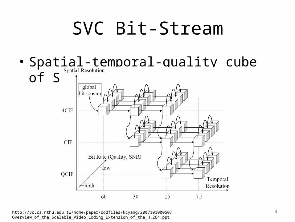
SVC Bit-Stream
• Spatial-temporal-quality cube of SVC
4http://vc.cs.nthu.edu.tw/home/paper/codfiles/kcyang/200710100050/Overview_of_the_Scalable_Video_Coding_Extension_of_the_H.264.ppt

RECEIVER DRIVEN LAYERED MULTICAST WITH LAYER-AWARE FORWARD ERROR CORRECTION
C. Hellge, T. Schierl, and T. Wiegand
ICIP 2008
5
C. Hellge, T. Schierl, and T. Wiegand, “MOBILE TV USING SCALABLE VIDEO CODING AND LAYER-AWARE FORWARD ERROR CORRECTION,” ICME 2008.C. Hellge, T. Schierl, and T. Wiegand, “Multidimensional Layered Forward Error Correction using Rateless Codes,” ICC 2008.

SVC Bit-Stream
• Equal FEC
6
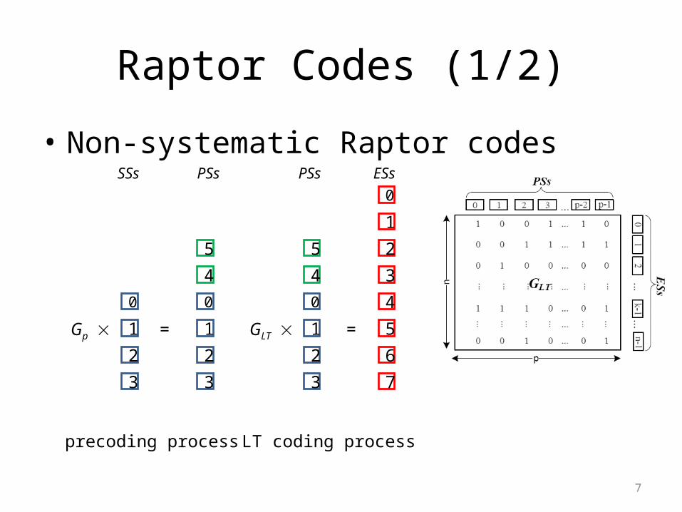
Raptor Codes (1/2)
• Non-systematic Raptor codes
0
1
2
3
0
1
2
3
4
5
Gp
0
1
2
3
4
5
GLT
0
1
2
3
4
5
6
7
= =
7
precoding process LT coding process
SSs PSs PSs ESs
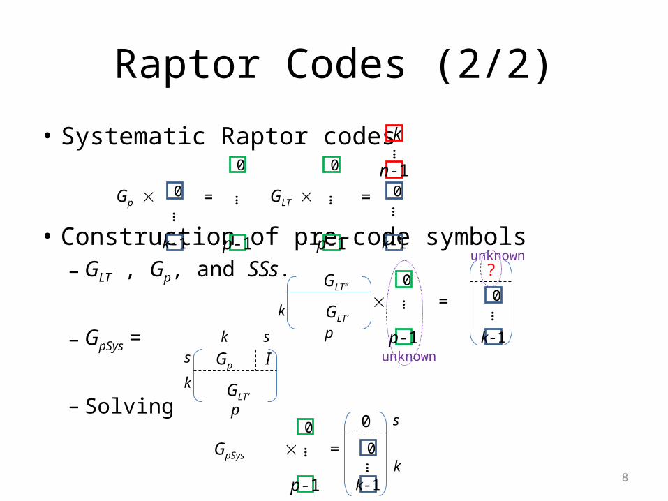
Raptor Codes (2/2)
• Systematic Raptor codes
• Construction of pre-code symbols– GLT , Gp, and SSs.
– GpSys =
– Solving
0 0
k
n-1
Gp GLT = =
0 0
GpSys =0
p-1
0
k-1
0
…
…
k-1 p-1 p-1 k-1
…
… …
……
GLT’
GLT’’
k 0
p-1
…
p
s
k
0
k-1
…
?
=
8
unknown
unknown
Gp I
GLT’
s
k
k s
p

Layer-Aware FEC (1/5)
• Example 1
• Example 2
9
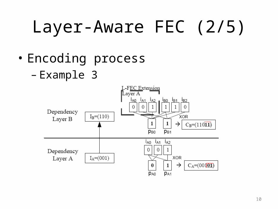
Layer-Aware FEC (2/5)
• Encoding process– Example 3
10
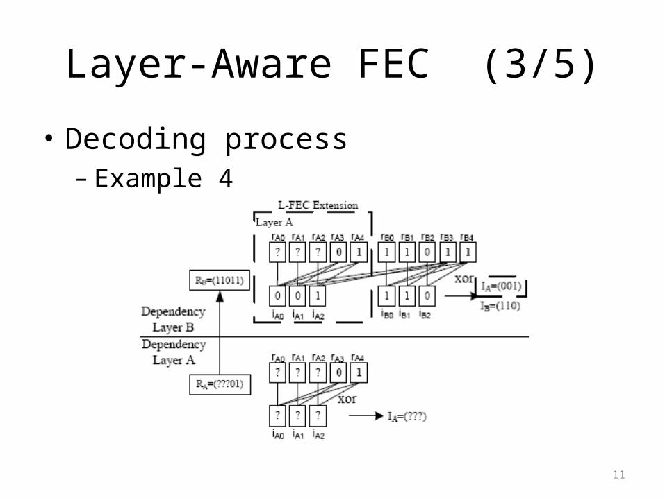
Layer-Aware FEC (3/5)
• Decoding process– Example 4
11
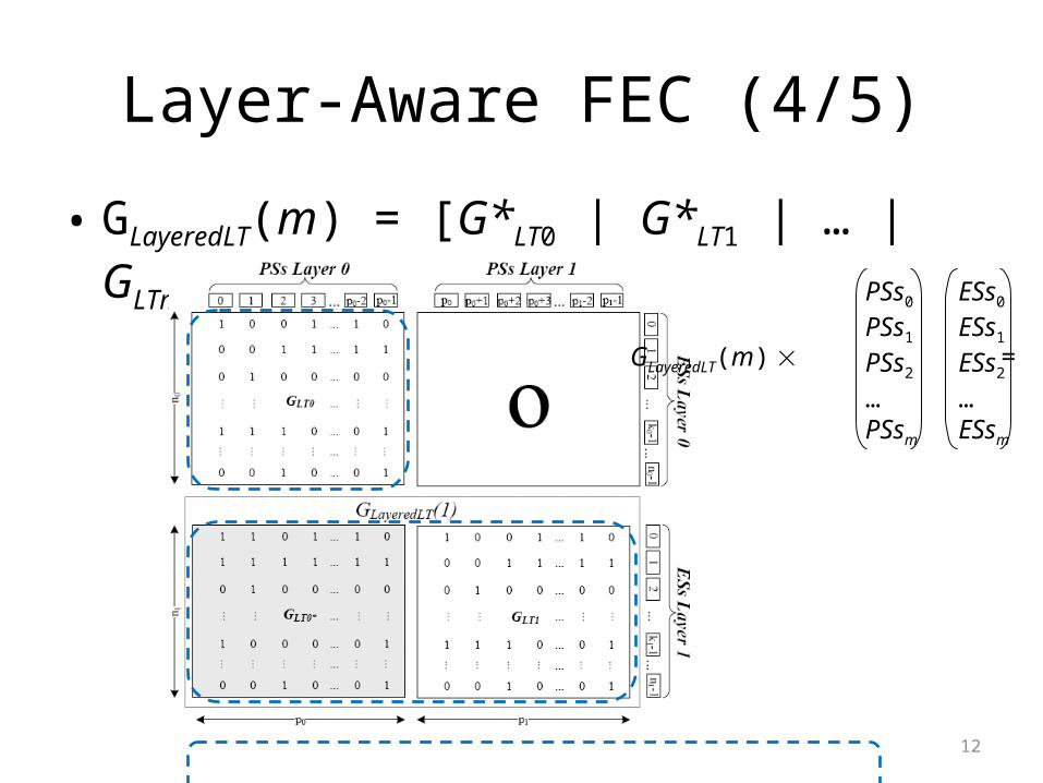
Layer-Aware FEC (4/5)
• GLayeredLT(m) = [G*LT0 | G*LT1 | … | GLTm]
12
GLayeredLT(m) =
PSs0
PSs1
PSs2
…PSsm
ESs0
ESs1
ESs2
…ESsm

Layer-Aware FEC (5/5)
• GpSysLayered(m)
13
0
SS0
0
SS1
0
GpSysLayered(m) =
PSs0
PSs1
PSs2
…PSsm
0
ESs0 0
ESs1…
0
ESsm
Simulation Results (1/2)
• QVGA (BL) and VGA (EL) resolution using SVC over a DVB-H channel.– JSVM 8.8– GOP size = 16
• Size of a transmission block = 186 bytes• Mean error burst length = 100 TBs
14

Simulation Results (2/2)
15

Joint Rate-Distortion Optimization of Transform
Coefficients For Spatial Scalable Video Coding Using SVC
M. Winken, H. Schwarz, and T. Wiegand
ICIP 200816

Hybrid Video Decoding
17
1 2
3 4
5 6
7 8
s5
s6
s7
s8
s2
s3
½ (s2+s3)sx
u5
u6
u7
u8
s1
s2
s3
s4
s5
s6
s7
s8
0000c5
c6
c7
c8
s1
s2
s3
s4
000sx
0 0 0 0 0 0 0 00 0 0 0 0 0 0 00 0 0 0 0 0 0 00 0 0 0 0 0 0 00 1 0 0 0 0 0 00 0 ½ ½ 0 0 0 0 0 1 0 0 0 0 0 00 0 0 0 0 0 0 0
s1
s2
s3
s4
s5
s6
s7
s8
0 0 0 0 0 0 0 00 0 0 0 0 0 0 00 0 0 0 0 0 0 00 0 0 0 0 0 0 00 0 0 0 ? ? ? ?0 0 0 0 ? ? ? ? 0 0 0 0 ? ? ? ?0 0 0 0 ? ? ? ?
= + +
= +
Motion compensatedvalues
Dequantized residual
Decoded pixel values
Motion vectors DeQuntized andiDCT parameters
Motion compensation iQ and iDCT Exception
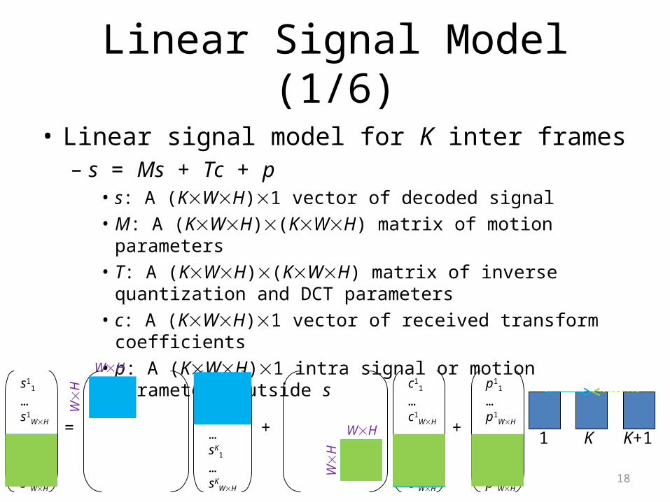
Linear Signal Model (1/6)
• Linear signal model for K inter frames– s = Ms + Tc + p
• s: A (KWH)1 vector of decoded signal• M: A (KWH)(KWH) matrix of motion parameters• T: A (KWH)(KWH) matrix of inverse quantization
and DCT parameters• c: A (KWH)1 vector of received transform coefficients• p: A (KWH)1 intra signal or motion parameters outside
s s11
…s1
WH
…sK
1
…sK
WH
s11
…s1
WH
…sK
1
…sK
WH
c11
…c1
WH
…cK
1
…cK
WH
p11
…p1
WH
…pK
1
…pK
WH
= + +1 K K+1
18
WH
W
H
WH
W
H

Linear Signal Model (2/6)
• Optimal transform coefficients selection– Decoder receives MVs (M) and quantized
transform coefficients (c).– fixed motion parameters (M), quantization
parameters (T), and intra predictions (p).• Rate and distortion are mainly controlled by c.
– c’ = argminc{D(c) + R(c)}
subject to s = Ms + Tc + p• D(c) = ||x - s||2
2, R(c) = ||c||1
19

Linear Signal Model (3/6)
• Optimal transform coefficients selection– Problem: MVs cannot be determined before the
transform coefficients are selected (trade-off)– Solution:
20
s11
…s1
WH
s21
…s2
WH
s31
…s3
WH
…sK
1
…sK
WH
c11
…c1
WH
c21
…c2
WH
c31
…c3
WH
…cK
1
…cK
WH
p11
…p1
WH
p21
…p2
WH
p31
…p3
WH
…pK
1
…pK
WH
= + +
s11
…s1
WH
s21
…s2
WH
s31
…s3
WH
…sK
1
…sK
WH
fixed
fixed
initial
initial
initial
initial

Linear Signal Model (4/6)
• Optimal transform coefficients– Problem size: K W H
• Sliding window approach (Reduce problem size)– s = M s + T c + p
21
window size
step size
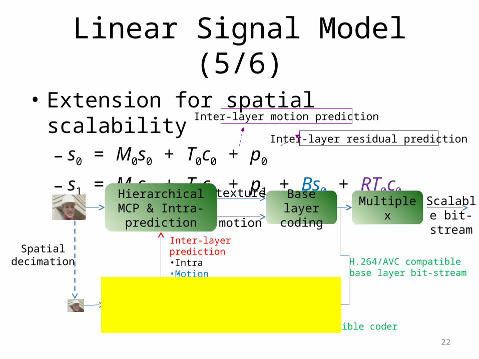
Linear Signal Model (5/6)
• Extension for spatial scalability– s0 = M0s0 + T0c0 + p0
– s1 = M1s1 + T1c1 + p1 + Bs0 + RT0c0
H.264/AVC MCP & Intra-prediction
Hierarchical MCP & Intra-prediction
Base layer coding
Base layer coding
texture
motion
texture
motion
Inter-layer prediction•Intra•Motion•Residual
Spatial decimation
Multiplex Scalable bit-stream
H.264/AVC compatible coder
H.264/AVC compatible base layer bit-stream
22
Inter-layer motion prediction
Inter-layer residual prediction

Linear Signal Model (6/6)
• Optimal transform coefficients in spatial scalability– c0’ D0(c0) + 0R(c0)
c1’ D1(c0,c1) + 1(R(c0)+R(c1))
subject to s0 = M0s0 + T0c0 + p0
s1 = M1s1 + T1c1 + p1 + Bs0 + RT0c0
c0’ (1-w)(D0(c0) + 0R(c0)) +
c1’ w(D1(c0,c1) + 1(R(c0)+R(c1)))
where = (W1H1)/(W0H0)
= argminc0’c1’
23
= argminc0’c1’

Description of the Algorithm
• Determine M0, T0, M1, T1, B, p0, R, and p1 by encoding the first K pictures using SVC reference encoder model.
• Solve optimization to determine c0 of the base layer.
• Based on new c0, determine B and R again.
• Solve optimization problem for only the enhancement layer.
24

Experimental Results (1/2)
• JSVM 9.9– IPPP– QCIF (base layer) and CIF (enhancement layer)– CABAC– QP difference: 3– Sliding windows size: 55 for base layer and
1010 for enhancement layer
25

Experimental Results (2/2)
26